Lie Groups and Lie Algebras in Particle Physics

Joao G. Rosa

Department of Physics and CIDMA, University of Aveiro & Department of Physics and Astronomy, University of Porto

These notes are part of a 12 hour lecture course given at the University of Porto, Portugal, to Physics Masters students.

The course is part of a larger curricular unit on Mathematical Methods in Physics, which includes a previous part on

discrete groups and applications to Condensed Matter Physics. I will nevertheless try to make these notes as self-contained

as possible, recalling where necessary some of the concepts and results that were taught in the previous part of the course.

These notes are not meant as an extensive review of Lie groups and Lie algebras, and for those interested in learning more

about the mathematical aspects of group theory and applications to particle physics I recommend the following textbooks:

• Howard Georgi, Lie algebras in particle physics (Westview Press, 1999).

• J. Fuchs and C. Schweigert, Symmetries, Lie Algebras and Representations (Cambridge University Press, 2003).

I am indebted to my PhD student Catarina Cosme for her help in typing part of these notes.

Contents

1 General properties of Lie Groups and Lie Algebras 2

1.1 Example: the Lie group SU (2) . . . . . . . . . . . . . . . . . . . . . . . . . . . . . . . . . . . . . . . . . . . 11

1.2 Cartan-Weyl basis . . . . . . . . . . . . . . . . . . . . . . . . . . . . . . . . . . . . . . . . . . . . . . . . . . 14

1.3 Example: the Cartan-Weyl basis for SU(2) . . . . . . . . . . . . . . . . . . . . . . . . . . . . . . . . . . . . 18

2 Lorentz and Poincare groups 20

2.1 Lorentz group . . . . . . . . . . . . . . . . . . . . . . . . . . . . . . . . . . . . . . . . . . . . . . . . . . . . . 20

2.1.1 Relation with SL(2,C) . . . . . . . . . . . . . . . . . . . . . . . . . . . . . . . . . . . . . . . . . . . . 22

2.1.2 Representations of the Lorentz group . . . . . . . . . . . . . . . . . . . . . . . . . . . . . . . . . . . . 24

2.1.3 Spinor bilinears . . . . . . . . . . . . . . . . . . . . . . . . . . . . . . . . . . . . . . . . . . . . . . . . 27

2.1.4 Parity and charge conjugation . . . . . . . . . . . . . . . . . . . . . . . . . . . . . . . . . . . . . . . 28

2.2 Poincare group . . . . . . . . . . . . . . . . . . . . . . . . . . . . . . . . . . . . . . . . . . . . . . . . . . . . 29

2.2.1 Massive representations . . . . . . . . . . . . . . . . . . . . . . . . . . . . . . . . . . . . . . . . . . . 32

2.2.2 Massless representations . . . . . . . . . . . . . . . . . . . . . . . . . . . . . . . . . . . . . . . . . . . 32

3 SU(N) groups 34

3.1 Irreducible representations of SU(N) . . . . . . . . . . . . . . . . . . . . . . . . . . . . . . . . . . . . . . . . 35

3.2 SU(3) and the quark model . . . . . . . . . . . . . . . . . . . . . . . . . . . . . . . . . . . . . . . . . . . . . 40

3.3 Branching SU(3) representations into SU(2) representations . . . . . . . . . . . . . . . . . . . . . . . . . . . 44

4 Problems 46

1

1 General properties of Lie Groups and Lie Algebras

Let us start by recalling the mathematical properties of a group:

DEFINITION: A group G is a set with a map G × G −→ G known as group multiplication satisfying the following

properties:

• Associativity: (g.h) .l = g. (h.l), ∀g,h,l∈G ,

• Identity: ∃e∈G e.g = g, ∀g∈G ,

• Inverse: ∀g∈G ∃g′∈G g′.g = g.g′ = e .

In particle physics we are mostly interested in representations of a group, which define the concrete realization of group

transformations. A group representation R is a map that associates to each group element a linear transformation

acting on a particular (real or complex) vector space, V :

R : G→ GL(V ) . (1)

The dimension of the representation corresponds to the dimension of the associated vector space. A representation is

reducible if and only if there is a subspace U ⊂ V left invariant by group transformations, i.e. R(g)u ∈ U for all u ∈ Uand g ∈ G. It is otherwise called irreducible and these are the representations that will mostly interest us in particle

physics applications.

A Lie Group is a continuous group, i.e. in which all elements g ∈ G depend continuously on a continuous set of

parameters

g = g (α) , α = {αa} , a = 1, ..., N . (2)

We can assume, without loss of generality, that the identity element corresponds to the origin in the space of parameters:

e = g (α) |α=0 , (3)

such that for any representation of the group:

R (α) |α=0= I . (4)

In a neighbourhood of the identity element, we may then expand R (α) in a Taylor series:

R (dα) = I + iXadαa + . . . , (5)

where we consider Einstein’s summation rule that repeated indices should be summed over. In the above expression we

have defined:

Xa ≡ −i∂

∂αaD (α) |α=0 , (6)

and used the notation dαa to denote an infinitesimal change in the {αa} parameters, thus obtaining a representation of a

group element arbitrarily close to the identity.

The {Xa} vectors are known as group generators. We include a factor i in their definition such that, for unitary

representations, R† (α)R (α) = I, the group generators are hermitian operators X†a = Xa as we will see below.

Group multiplication then allows us to obtain any other finite element of the group by multiplying (5) by an infinitesimal

2

transformation an arbitrary number of times:

R (α) = limk→∞

(I + i

αaXa

k

)k= exp (iαaXa) , (7)

where dαa = limk→∞αak . This defines the exponential map or exponencial parametrization of the group elements.

We may thus write the group elements in terms of its generators, at least in a neighbourhood of the identity. For a

unitary representation, eiαaXae−iαaX†a = I, which implies Xa = X†a as anticipated. As opposed to the group elements, the

generators form a linear vector space and any linear combination of the generators is itself a group generator.

Let us consider a one-parameter family of group elements given by:

U (λ) = exp (iλαaXa) . (8)

In this case, group multiplication is quite simple and yields:

U (λ1)U (λ2) = exp (iλ1αaXa) exp (iλ2αaXa)

= exp (i (λ1 + λ2)αaXa) (9)

= U (λ1 + λ2) .

However, for group elements that are generated by different linear combinations of the generators this is not so simple,

since in general:

exp (iαaXa) exp (iβbXb) 6= exp (i (αa + βb)Xa) . (10)

Since any group element admits a parametrization in terms of the exponential map, we must have that:

exp (iαaXa) exp (iβbXb) = exp (iδaXa) , (11)

for some set of parameters {δa}, a = 1, ..., N . Continuity and differentiability of the group elements then allows us to find

the {δa} parameters by expanding both sides of Eq. (11) in a Taylor series. We first note that:

iδaXa = ln [1 + exp (iαaXa) exp (iβbXb)− 1] ≡ ln (1 +K) , (12)

and that, for small K,

ln (1 +K) = K − K2

2+ . . . (13)

Thus, expanding up to to quadratic order in the αa and βa parameters:

K = exp (iαaXa) exp (iβbXb)− 1

=

(1 + iαaXa −

1

2(αaXa)

2+ . . .

)(1 + iβbXb −

1

2(βbXb)

2+ . . .

)− 1

= iαaXa + iβaXa − αaXaβbXb −1

2(αaXa)

2 − 1

2(βaXa)

2+ . . . (14)

Hence, we have that:

iδaXa = iαaXa + iβaXa − αaXaβbXb −1

2(αaXa)

2 − 1

2(βaXa)

2+

1

2(αaXa + βaXa)

2+ . . .

= i (αa + βa)Xa − αaXaβbXb +1

2αaXaβbXb +

1

2βbXbαaXa + . . .

= i (αa + βa)Xa −1

2[αaXa, βbXb] + . . . , (15)

3

where we have taken into account that the generators are linear operators that do not, in general, commute with each

other. We thus find that:

[αaXa, βbXb] = −2i (δc − αc − βc)Xc + . . . ≡ iγcXc + . . . (16)

Since this must hold for any choice of parameters, we conclude that:

γc = fabcαaβb (17)

and that, hence,

[Xa, Xb] = ifabcXc , (18)

where the constants satisfy:

fabc = −fbac, (19)

since the commutator is antisymmetric, [A,B] = − [B,A] . These are known as the group’s structure constants and

define the Lie algebra of the the group G, L(G), i.e. the set of generators with the closed commutation properties above.

The commutator (18) defines the fundamental properties of the Lie algebra and thus plays a similar role to the group

multiplication. We thus conclude that:

δa = αa + βa −1

2γa + . . . (20)

which implies:

exp (iαaXa) exp (iβbXb) = exp

(i (αa + βa)Xa −

1

2[αaXa, βbXb] + . . .

), (21)

which is known as the Baker-Campbell-Hausdorff (BCH) relation. The higher-order terms that we have discarded

above correspond to commutators of commutators, e.g. [αaXa, [αcXc, βbXb]] and are thus determined by the structure

constants. Hence, the Lie algebra (18) is sufficient to completely define the group multiplication in a finite neighbourhood

of the identity.

The structure constants are an intrinsic property of the Lie algebra and are independent of its representation, being

determined solely by the group multiplication rule and by continuity. Each representation of the group then defines a

representation of the associated Lie algebra. A useful property to note is that the structure constants are real if there is

a unitary group representation.

DEM: Since in a unitary group representation the generators are hermitian operators we have, on the one hand, that:

[Xa, Xb]†

= −if∗abcX†c = −if∗abcXc ,

and, on the other hand, that:

[Xa, Xb]†

= (XaXb)† − (XaXb)

†

= XbXa −XaXb

= − [Xa, Xb]

= −ifabcXc.

so that fabc = f∗abc. Q.E.D.

The group generators satisfy the Jacobi identity:

[Xa, [Xb, Xc]] + [Xb, [Xc, Xa]] + [Xc, [Xa, Xb]] = 0 . (22)

4

This can be shown in a straightforward way by expanding all the commutators, so we leave it as an exercise.

The structure constants themselves can be used to define an important representation of the Lie algebra known as the

adjoint representation. This can be done by defining the N ×N matrices

[Ta]bc ≡ −ifabc , (23)

the commutator of which is given by:

[Ta, Tb]cd = (TaTb − TbTa)cd

= (Ta)ce (Tb)ed − (Tb)ce (Ta)ed

= −facefbed + fbcefacd . (24)

From the Jacobi identity we have that:

[Xa, [Xb, Xc]] = [Xa, ifbcdXd]

= ifbcd [Xa, Xd]

= −fbcdfadeXe , (25)

and so

(fbcdfade + fcadfbde + fabdfcde)Xe = 0 ∀Xe∈L(G)

⇒ fbcdfade + fcadfbde + fabdfcde = 0 . (26)

If we now interchange the indices d and e, we obtain:

−facefbed + fbcefaed = −fabefced , (27)

from which we conclude that:

[Ta, Tb]cd = −fabefced= fabefecd

= ifabe (Te)cd ,

which can be written as:

[Ta, Tb] = ifabcTc , (28)

such that the Ta matrices satisfy the commutation relation of the Lie algebra in Eq. (18). The dimension of the adjoint

representation corresponds to the number of independent generators, i.e. to the number of (real) parameters required

to specify a group element. Note that the generators are pure imaginary matrices in the adjoint representation if the

structure constants are real.

A more formal way of defining the adjoint representation is given by the map:

ad : L (G)→M (L (G))

ad (X) (Y ) = [X,Y ] , X, Y ∈ L(G). (29)

5

We may write this in components by choosing a basis of generators for the Lie algebra {Ta}, a = 1, ..., N :

ad (Ta) (Tb) = [Ta, Tb] = ifabcTc

⇒ ad (Ta)cb = ifabc = − [Ta]bc = [Ta]cb ,

in agreement with the definition above. Note that we have used that fabc = −facb as we will show explicitly below.

The adjoint representation of the Lie algebra naturally induces a representation of the group, also known as the adjoint

representation of the group:

Ad : G→ GL (L (G))

Ad (g)Ta = gTag−1 , g ∈ G,Ta ∈ L(G) . (30)

We can easily check that these two representations are related through the exponential map. Writing a group element as

g = exp (iαaTa), we have that:

Ad (g) (Ta) = exp (iαbTb)Ta exp (−iαbTb)= (1 + iαbTb + . . .)Ta (1− iαbTb + . . .)

= Ta + iαb [Tb, Ta] + . . .

= Ta + iαbad (Tb) (Ta) + . . .

= exp (iαbad (Tb) (Ta)) . (31)

Let us now introduce a series of definitions and theorems that can be used to classify different Lie algebras.

DEFINITION: A sub-algebra A ⊂ L (G) is a linear space such that:

∀X,Y ∈A [X,Y ] ∈ A . (32)

We can highlight the following special cases of sub-algebras:

• A sub-algebra is abelian if:

∀X,Y ∈A, [X,Y ] = 0 , (33)

and the same applies naturally to the full Lie algebra L(G).

• A sub-algebra is an ideal if:

∀X∈A∀Z∈L(G) [X,Z] ∈ A , (34)

and a proper ideal if, in addition, A 6= L (G) , {0} .

DEFINITION: A Lie algebra is simple if it does not contain any proper ideals and semi-simple if it does not contain

abelian ideals except {0}.

6

THEOREM: A Lie algebra is semi-simple if and only if:

L = L1 ⊕ ...⊕ LN (35)

where Li, i = 1, ..., N , are simple algebras.

A rigorous proof of this theorem is out of the scope of these lectures, but let us consider a generic example that

illustrates these general definitions and properties. Consider the product of two groups G = G1 × G2, where the Lie

algebras L(G1) and L(G2) are simple, i.e. have no proper ideals as defined above. We can write a generic element of G in

the matrix form:

g =

(g1 0

0 g2

)∈ G ,

for gi ∈ Gi, i = 1, 2, such that the elements of the Lie algebra, i.e. the generators, can be written as:

T =

(T1 0

0 T2

)∈ L (G) .

Let us then consider the sub-algebra L(G1) with elements of the form:

T ′ =

(T ′1 0

0 0

).

Then, we have for the commutator between a generic element of L(G) and an element of this sub-algebra:

[T, T ′] =

(T1 0

0 T2

)(T ′1 0

0 0

)−(T ′1 0

0 0

)(T1 0

0 T2

)

=

(T1T

′1 0

0 0

)−(T ′1T1 0

0 0

)

=

(T ′′1 0

0 0

),

where T ′′1 = [T1, T′1] ∈ L (G1). Hence, the elements of the sub-algebra L(G1) constitute a proper ideal and L(G) cannot

be simple. It is easy to see, by a similar reasoning, that the elements of L(G2) also form a proper ideal, and that there

are no other ideals since L(G1) and L(G2) are simple algebras. Thus, the full Lie algebra L(G) = L(G1)⊕ L(G2) will be

semi-simple if these ideals are not abelian.

DEFINITION: The Killing form or Killing metric associated with a Lie algebra L (G) is a symmetric bilinear map:

Γ : L (G)× L (G) → R

defined by:

Γ (X,Y ) = Tr [ad (X) · ad (Y )] , X, Y ∈ L (G) . (36)

This defines an inner product within the Lie algebra in the adjoint representation. Considering a basis of generators

7

{Ta} for the Lie algebra we obtain for the Killing metric components:

γab = Γ (Ta, Tb) = Tr [TaTb] = (Ta)cd (Tb)dc = (−ifacd) (−ifbdc)= −facdfbdc . (37)

THEOREM: A Lie algebra is semi-simple if the Killing form is non-degenerate:

Γ (X,Y ) = 0 ∀X∈L(G) ⇒ Y = 0 ,

or equivalently that det(γ) 6= 0.

DEM: Let us suppose that Γ is non-degenerate and that A ⊂ L (G) is an abelian ideal. We can then choose a basis

{Ta, Tα} for the Lie algebra where Ta generate the elements in A and Tα correspond to the remaining generators of L (G).

Then, for X ∈ L (G) and Y ∈ A we have:

ad (X) · ad (Y ) (Ta) = [X, [Y, Ta]] = 0 ,

since [Y, Ta] = 0. Also:

ad (X) · ad (Y ) (Tα) = [X, [Y, Tα]] =∑

a

αaTa , (38)

since [Y, Tα] ∈ A and so [X, [Y, Tα]] ∈ A as well. We thus conclude that the Killing metric has the form:

Γ (X,Y ) = Tr [ad (X) · ad (Y )]

= Tr

[0 ∗0 0

]

= 0 .

Since by assumption Γ is non-degenerate, we must have Y = 0, and so there cannot exist any non-trivial abelian ideals

and the algebra is semi-simple. The proof in the opposite direction follow an analogous reasoning. Q.E.D.

THEOREM: If L (G) is a compact Lie algebra, i.e. if the underlying Lie group is compact, being defined in term of a

compact manifold of parameters, then the Killing form is positive semi-definite:

Γ (X,X) ≥ 0, ∀X∈L(G) , (39)

and if the algebra is simple, we have:

Γ (X,X) > 0, ∀X∈L(G) . (40)

Although we will not prove this theorem in this course, we can use it to show an important result that we have

anticipated above. If the Killing form is positive definite, then we can choose an orthonormal basis for the Lie algebra

such that:

Γ (Ta, Tb) = δab , (41)

which just means that we may diagonalize the Killing metric and choose an appropriate normalization for the generators.

8

In this basis, the structure constants are completely antisymmetric.

DEM:

Γ ([Tc, Ta] , Tb) + Γ (Ta, [Tc, Tb]) = Tr [(TcTa − TaTc)Tb] + Tr [Ta (TcTb − TbTc)]= Tr [TcTaTb]− Tr [TaTcTb] + Tr [TaTcTb]− Tr [TaTbTc]

= 0,

using the cyclic property of the trace. Thus,

Γ (ifcadTd, Tb) + Γ (Ta, ifcbdTd) = ifcadTr [TdTb] + ifcbdTr [TaTd] = ifcadδdb + ifcbdδad = fcab + fcba = 0 , (42)

so that fcab = −fcba. Since by the definition the structure constants are antisymmetric in the first two indices, this implies

that they must be completely antisymmetric. Q.E.D.

THEOREM: For a semi-simple Lie algebra the (quadratic) Casimir operator:

C ≡ γijTiTj , (43)

where γij = γ−1ij , commutes with all the generators:

[C, Tk] = 0 ∀Tk∈L(G) . (44)

DEM:

[C, Tl] = γij [TiTj , Tl]

= γijTi [Tj , Tl] + γij [Ti, Tl]Tj

= iγijTifjlmTm + iγijfilmTmTj

= iγijfjlmTiTm + iγijfjlmTmTi

= iγijfjlm (TiTm + TmTi)

= ifjlmγij (TiTm + TmTi)

= 0 ,

since fjlm is antisymmetric while γij (TiTm + TmTi) is symmetric under the interchange of the indices j and m, noting

that the Killing metric is symmetric. Q.E.D.

An important result in the theory of group representations is Schur’s Lemma, which can be cast in the following form:

SCHUR’S LEMMA: For an irreducible representation R of a group G over a complex vector space V , if there exists a

linear transformation P ∈ GL(V ) that commutes with the action of all group elements:

[P,R(g)] = 0 ∀g∈G , (45)

then this operator must be proportional to the identity, P = λI for some complex constant λ.

9

DEM: Consider the space of eigenvectors of the operator P with eigenvalue λ:

Eig(λ) = {v ∈ V : Pv = λv} . (46)

This must be a non-empty set for some λ since det(P − λI) = 0 has at least one solution in C. Then, for v ∈ Eig(λ) we

have that:

P (R(g)v) = R(g)(Pv) = λR(g)v , (47)

which implies that R(g)v ∈ Eig(λ), i.e. that the eigenspace is left invariant by the action of the group. Since, by assumption,

the representation is irreducible, than Eig(λ) = V , which implies that P = λI. Q.E.D.

It is easy to see that Schur’s Lemma applies to the irreducible representations of both a Lie group and its Lie algebra.

This then leads us to the conclusion that, in any irreducible representation r of L(G), the Casimir operator is proportional

to the identity:

C = C (r) Idim(r) , (48)

where C (r) is a number that is characteristic of the representation. In the orthonormal basis where γij = δij (for a simple

and compact Lie algebra), we have:

C = δijT(r)i T

(r)j =

∑

i

(T

(r)i

)2= C (r) Idim(r) . (49)

We may also consider the quadratic operator:

Mij = Tr[T

(r)i , T

(r)j

], (50)

for the Lie algebra generators in a given representation r. The commutator of this operator with a generator in the adjoint

representation is then given by:

([Ti,M ])jk = (Ti)jlMlk −Mjl (Ti)lk

= −ifijlTr[T

(r)l , T

(r)k

]+ ifilkTr

[T

(r)j , T

(r)l

]

= −Tr[[T

(r)i , T

(r)j

], T

(r)k

]− Tr

[T

(r)j

[T

(r)i , T

(r)k

]]

= −Tr[T

(r)i T

(r)j T

(r)k − T (r)

j T(r)i T

(r)k + T

(r)j T

(r)i T

(r)k − T (r)

j T(r)k T

(r)i

]

= 0 , (51)

using the cyclic property of the trace. Schur’s Lemma than implies that

M = C (r) Idim(ad) . (52)

The two Casimir constants C (r) and C (r) are thus related via:

Tr(r) (C) = C (r) dim (r)

=∑

i

Tr(T

(r)i

)2

= Tr(r) (M)

= C (r) dim (ad) , (53)

10

such that

C (r) =dim (r)

dim (ad)C (r) . (54)

We note, as an aside, that the Casimir operators play a very important role in particle physics, since they characterize

the irreducible representations in which each type of field transforms under symmetry operations associated with particular

Lie groups, as we will discuss in more detail later on.

1.1 Example: the Lie group SU (2)

To better understand the general concepts and definitions introduced in this section, let us look in detail into a particular

example, that of the group of 2 × 2 unitary matrices with unit determinant, denoted as SU(2). This will also serve as a

warm up exercise to the more detailed study of SU(N) representations and applications to particle physics that we will

do later on. The group is formally defined as

SU(2) ={U ∈ GL

(C2)

: U†U = I, det (U) = 1}.

For a generic matrix in this group:

U =

(a b

c d

)⇒ U† =

(a∗ b∗

c∗ d∗

).

The unitarity condition yields for the matrix components:

UU† =

(|a|2 + |b|2 ac∗ + bd∗

ca∗ + db∗ |c|2 + |d|2

)=

(1 0

0 1

)⇒

ac∗ + bd∗ = 0

a∗c+ b∗d = 0⇔

a = d∗

b = −c∗

This implies that a generic 2× 2 unitary matrix can be written in the form:

U =

(α β

−β∗ α∗

),

and the unit determinant condition yields:

det (U) = |α|2 + |β|2 = 1 .

The SU(2) group can thus be defined by:

SU(2) =

{(α β

−β∗ α∗

): α, β ∈ C , |α|2 + |β|2 = 1

},

such that each element of the group is specified by two complex numbers subject to a single real condition, thus having

three independent degrees of freedom.

To determine the associated Lie algebra, we consider infinitesimal group transformations (arbitrarily close to the

identity), U = I + iT + . . . to obtain that:

UU† = (I + iT + ....)(I− iT † + ....

)= I ⇒ T = T † .

11

and also that:

det (U) = det (I + iT + ....) = 1 + iTr(T ) = 1 ⇒ Tr (T ) = 0 .

Recall that for a generic matrix with eigenvalues λi, det (A) =∏i λi and Tr(A) =

∑i λi. If A ' I + X + . . . then

λi = 1 + εi + . . ., where εi are the arbitrarily small eigenvalues of X, such that det (A) =∏i(1 + εi) = 1 +

∑i εi + . . . =

1 + Tr (X), which we used above.

These results then imply that the Lie algebra of SU(2) is given by:

L (SU (2)) ={T ∈M

(C2)

: T = T †, Tr (T ) = 0}. (55)

A generic matrix in the SU(2) Lie algebra may then be written in the form:

T =

(a b

c d

)=

(a∗ c∗

b∗ d∗

),

which, along with the condition Tr(T ) = a+ d = 0, leads us to the conclusion that the diagonal entries must be real with

a = −d, while the non-diagonal entries are complex conjugate, leaving only three real degrees of freedom, in agreement to

what we found above for the group elements.

The basis of matrices for the SU(2) algebra is conventionally chosen to be given in terms of the three Pauli matrices,

Ti = σi/2, i = 1, 2, 3:

σ1 =

(0 1

1 0

), σ2 =

(0 −ii 0

), σ3 =

(1 0

0 −1

). (56)

It is easy to check that these matrices satisfy:

[σi, σj ] = 2iεijkσk , {σi, σj} = 2δij , σiσj = δij + iεijkσk , (57)

where the anti-commutator {A,B} = AB +BA. This thus implies that

[Ti, Tj ] = iεijkTk , (58)

such that the SU(2) structure constants are fijk = εijk in terms of the totally antisymmetric Levi-Civita tensor. In this

basis we also have that

Tr (TiTj) =1

4Tr (σiσj) =

1

4[δijTr (I) + iεijkTr (σk)] =

1

2δij .

We note that it is possible to choose the normalization of the generators such that Tr (TiTj) = δij but the above is the

most conventionally used normalization. The Killing metric for the SU(2) algebra is given by:

γij = −εiklεjlk = 2δij ,

12

as can be checked explicitly for the different components:

γ11 = −ε1klε1lk = − (ε123ε132 + ε132ε123) = 2

γ22 = −ε2klε2lk = − (ε213ε231 + ε231ε213) = 2

γ33 = −ε3klε3lk = − (ε312ε321 + ε321ε312) = 2

γ12 = −ε1klε2lk = 0

γ13 = −ε1klε3lk = 0

γ23 = −ε2klε3lk = 0 .

This yields det (γ) = 8 6= 0, so that the algebra is semi-simple. In fact, the SU(2) algebra is simple since there are no

proper ideals, as can be inferred from the commutation relations satisfied by the Pauli matrices.

The Pauli matrices define the fundamental representation of the SU(2) algebra, also known as the spin-1/2

representation. This representation acts on 2-dimensional vectors known as SU(2) doublets.

The adjoint representation (or spin-1 representation) is given by:

(T

(ad)i

)jk

= −ifijk = −iεijk ,

with generators:

T(ad)1 = i

0 0 0

0 0 1

0 −1 0

, T

(ad)2 = −i

0 0 −1

0 0 0

1 0 0

, T

(ad)3 = −i

0 1 0

−1 0 0

0 0 0

. (59)

Another important representation is the complex conjugate representation:

R∗ (U) = U∗ = eT∗,

where T = i∑j αjσj . We can use that σ∗i = −σ2σiσ2, as can be explicitly checked:

σ2σ1σ2 = σ2 (iε123σ3) = iε123 (iε231)σ1 = −σ1 ,σ2σ2σ2 = σ2 ,

σ2σ3σ2 = σ2 (iε321σ1) = iε321 (iε213)σ3 = −σ3 ,

to show that:

σ2Tσ2 = i (−α1σ1 + α2σ2 − α3σ3)

= −i (α1σ∗1 + α2σ

∗2 + α3σ

∗3)

= T ∗ .

This then implies that:

R∗(U) = eσ2Tσ2 = eσ2Tσ−12 .

13

Now note that, for generic matrices A and B:

eABA−1

=∑

n

(ABA−1

)n

n!,

and that

(ABA−1

)n=(ABA−1

) (ABA−1

)...(ABA−1

)= ABnA−1 ,

so that we have:

eABA−1

= A

(∑

n

Bn

n!

)A−1 = AeBA−1 .

Using this result, we may write the complex conjugate representation in the form:

R∗ (U) = σ2eTσ−12 = σ2R(U)σ−12 .

Hence, the fundamental and complex conjugate representations are not really independent and, in fact, are said to be

equivalent. The fundamental representation is then said to be pseudo-real.

1.2 Cartan-Weyl basis

To define the Cartan-Weyl basis, which is extremely useful in determining and classifying representations of Lie groups

and associated algebras, we will consider semi-simple Lie algebras with generators {Ti} , i = 1, ..., N . Let us take a linear

combination of the generators:

H = aiTi ∈ L , (60)

where we use the Killing metric γij and its inverse γij to lower and raise indices, such that the Einstein summation

convention requires repeated upper and lower indices to be summed over. Note that in the previous calculations we

worked with lower indices exclusively, which is consistent in the Lie algebra basis where the Killing metric is the identity.

However, as we will see in the Cartan-Weyl basis this does not hold and we must use this more correct version of the

summation convention.

With the linear combination of generators above, we can study the eigenvalue problem:

ad (H) (T ) = [H,T ] = ρT . (61)

This can be written in components on the given basis as:

[aiTi, Tj

]= ρTj ⇔ aif k

ij Tk = ρTj

⇔(aif k

ij − ρδ kj

)Tk = 0

⇒ det(aif k

ij − ρδ kj

)= 0 ,

where the structure constants are now defined as:

[Ti, Tj ] = f kij Tk .

14

CARTAN’S THEOREM

Choosing the linear combination H with the largest possible number of eigenvalues ρ:

1. The eigenvalue ρ = 0 can be degenerate with multiplicity l = rank(L) and the corresponding eigenspace is generated

by {Hi}, i = 1, . . . , l, such that

[Hi, Hj ] = 0 . (62)

2. All the non-vanishing eigenvalues ρ 6= 0 are non-degenerate.

The proof of Cartan’s Theorem is out of the scope of this course, but we can study its implications. First, we can

immediately conclude that:

[H,Hi] = 0 ,

[H,Eα] = αEα, α 6= 0 . (63)

Now, since [H,H] = 0, we must have H = λiHi. In addition, the Jacobi identity implies that:

[H, [Hi, Eα]] = − [Hi, [Eα, H]]− [Eα, [H,Hi]]

= α [Hi, Eα] ,

which means that [Hi, Eα] is an eigenvector of H with eigenvalue α 6= 0 which, by Cartan’s Theorem, is non-degenerate.

Hence:

[Hi, Eα] = αiEα . (64)

Therefore, we have that:

[H,Eα] = λi [Hi, Eα] = λiαiEα = αEα (65)

from which we infer the relation α = λiαi. We may then write the structure constants in the form:

[Hi, Eα] = f βiα Eβ ⇒ f β

iα = αiδβ

α . (66)

We may further consider the Jacobi identity for the generators H, Eα and Eβ :

[H, [Eα, Eβ ]] + [Eβ , [H,Eα]] + [Eα, [Eβ , H]] = 0

[H, [Eα, Eβ ]] + α [Eβ , Eα]− β [Eα, Eβ ] = 0

[H, [Eα, Eβ ]] = (α+ β) [Eα, Eβ ] , (67)

such that [Eα, Eβ ] is an eigenvector of H with eigenvalue α+ β. This leads to two possible commutation relations:

[Eα, Eβ ] = NαβEα+β , α+ β 6= 0

[Eα, E−α] = f iα−α Hi , α+ β = 0

. (68)

This yields the structure constants:

f γαβ = Nαβδ

γα+β . (69)

15

Having found the form of the structure constants in the basis {Hi, Eα}, we may compute the components of the Killing

metric in this basis:

γiα = −f γiβ f β

αγ

= −αiδ γβ Nαγδ

βα+γ

= −αiNαβδ βα+β

= 0 , (70)

since α 6= 0, or also since Nαβ is anti-symmetric and δ βα+β is symmetric under the exchange of the indices α and β.

Similarly, we obtain:

γαβ = −f µαγ f γ

βµ

= −Nαγδ µα+γ Nβµδ

γβ+µ

= −NαγNβ,α+γδ γβ+α+γ . (71)

This implies that γαβ 6= 0 if and only if α+ β = 0. We may then choose to normalize the Eα generators such γα−α = 1.

Finally, we have:

γij = −f βiα f α

jβ

= −αiδ βα αjδ

αβ

= −αiαjδ αα

= −∑

α

αiαj . (72)

This result allows to derive the remaining structure constants:

f iα−α = γijfα−αj

= γijfjα−α

= γijf βjα γβ−α

= γijf αjα

= γijαj

= αi . (73)

Let us summarize the above results. Cartan’s Theorem allows us to find a basis for a semi-simple Lie algebra {Hi, Eα},i = 1, ..., l = rank (L), known as the Cartan-Weyl basis, with the following commutation relations:

[Hi, Hj ] = 0

[Hi, Eα] = αiEα

[Eα, Eβ ] = NαβEα+β , α+ β 6= 0

[Eα, E−α] = αiHi , (74)

The abelian sub-algebra spanned by {Hi} is known as Cartan’s sub-algebra. The vectors α = (αi)i=1,...,l are denoted

16

as the root vectors. In this basis the Killing metric takes the form:

γij = −∑

α

αiαj

γiα = 0

γα−α = 1

γαβ = 0 , α+ β 6= 0 . (75)

In the Cartan-Weyl basis, we can find an SU(2) sub-algebra. To see this, let us start by choosing H = αiHi for a

given root vector α. The subset of generators {H,Eα, E−α} for each root vector α then satisfies the closed algebra:

[H,Eα] = αi [Hi, Eα] = αiαiEα

[H,E−α] = αi [Hi, E−α] = −αiαiE−α[Eα, E−α] = αiHi = H . (76)

To see that this is an SU(2) algebra, note that defining σ± = σ1 ± iσ2 and using the commutation relations for the Pauli

matrices, we have:

[σ±, σ3] = [σ1, σ3]± i [σ2, σz] = −σ2 ± iσ1 ± i (σ1 ± iσ2) = ±iσ±[σ+, σ−] = [σ1 + iσ2, σ1 − iσ2]− i [σ1, σ2] + i [σ2, σ1] = −2iσ3 , (77)

which has the same form as Eq. (76) identifying H ↔ σ3 and E±α ↔ σ±.

Let us now consider a representation r of the Lie algebra on a vector space V . Let us choose a basis {|λ〉} for V such

that:

H(r)i |λ〉 = λi|λ〉 , (78)

where we note that since all Hi generators in the Cartan sub-algebra commute they have a common eigenspace. The

l-dimensional vectors λ = (λ1, λ2, . . . , λl) are then designated as weight vectors of a given representation. Now, note

that:

Hi (Eα|λ〉) = EαHi|λ〉+ [Hi, Eα]|λ〉= λiEα|λ〉+ αiEα|λ〉= (λi + αi) (Eα|λ〉) , (79)

such that Eα|λ〉 is an eigenvector of Hi with eigenvalue λi + αi, i.e. with weight vector λ+ α. We thus see that the E±αgenerators act as raising and lowering operators in a given representation and can be used to find all the weights in the

representation.

For the adjoint representation, where the vector space V coincides with the Lie algebra itself, we have:

ad(Hi)(Hj) = [Hi, Hj ] = 0 ,

ad(Hi)(Eα) = [Hi, Eα] = αiEα . (80)

This means that the eigenstates corresponding to the generators Hi have null weights, while for the eigenstates Eα the

weights coincide with the roots of the Lie algebra.

For tensor representations of the group R(g) = R1(g) × R2(g) and associated representations of the Lie algebra, we

17

have:

H(1)i |λ〉 = λi|λ〉 , H

(2)i |µ〉 = µi|µ〉 , (81)

such that

Hi(|λ〉 ⊗ |µ〉) =(H

(1)i |λ〉

)⊗ |µ〉+ |λ〉 ⊗

(H

(2)i |µ〉

)

= (λi + µi)|λ〉 ⊗ |µ〉 , (82)

such that the weights of tensor representations correspond to the sum of the weights of the individual representations.

1.3 Example: the Cartan-Weyl basis for SU(2)

To illustrate the advantages of using the Cartan-Weyl basis, let us return to our SU(2) example, which is a rank 1

Lie algebra, i.e. there is only one generator in the Cartan sub-algebra. Recalling that the basis of generators in the

fundamental representation is Ti = σi/2 , i = 1, 2, 3, we can take H = T3 corresponding to the diagonal generator and

define E± = (T1 ± iT2)/2, such that:

[H,E±] = ±E± , [E+, E−] =1

2H . (83)

Thus, the SU(2) algebra has roots α± = ±1. For a given SU(2) representation we label the states in the associated vector

space basis as |j,m〉, where m denotes the weights of the representation:

H|j,m〉 = m|j,m〉 (84)

and the spin j = max(m) is the highest weight in the representation, which is then denoted as a spin-j representation.

For the fundamental representation, the eigenvalues of H = σ3/2 are ±1/2, so that the fundamental representation is the

spin-1/2 representation as mentioned earlier. The adjoint representation has three weights, m = 0,±1 as can be inferred

explicitly from the form of the adjoint generators in Eq. (59), thus corresponding to the spin-1 representation.

For a generic spin-j representation, we can obtain all the states in the basis using the raising and lowering operators

E±. It is conventional to use instead the raising and lowering operators J± = 2E±, and from our discussion in the previous

sub-section we must have:

J−|j,m〉 = Nm|j,m− 1〉 , J+|j,m− 1〉 = Nm|j,m〉 , (85)

with constants Nm that we wish to determine. On the one hand, we have that:

〈j,m|J+J−|j,m〉 = ||J−|j,m〉||2 = |Nm|2〈j,m− 1|j,m− 1〉 = |Nm|2 , (86)

assuming that the states are normalized. On the other hand, we also have that:

〈j,m|J+J−|j,m〉 = 〈j,m|[J+, J−]|j,m〉+ 〈j,m|J−J+|j,m〉= 〈j,m|2H|j,m〉+ |Nm+1|2

= 2m+ |Nm+1|2 . (87)

This then yields the recurrence relation:

|Nm|2 = 2m+ |Nm+1|2 , (88)

18

with boundary condition Nj+1 = 0 since by definition j is the highest weight and J+|j, j〉 = 0. It is easy to verify that

the solution is then:

Nm =√j(j + 1)−m(m− 1) , (89)

such that

J+|j,m〉 =√j(j + 1)−m(m+ 1)|j,m+ 1〉 ,

J−|j,m〉 =√j(j + 1)−m(m− 1)|j,m− 1〉 . (90)

In particular, J−|j,−j〉 = 0, such that the weights in each spin-j representation are m = −j,−j + 1, . . . , j − 1, j, being a

(2j + 1)-dimensional representation.

For each spin-j representation, the Casimir operator is then given by:

C =1

2

∑

i

T 2i =

1

2H2 +

1

4J+J− +

1

4J−J+ . (91)

As we have seen, Schur’s Lemma implies that this is proportional to the identity, and to obtain the proportionality constant

we can take the trace of the Casimir operator in a given representation:

Trj(C) =∑

m

〈j,m|(

1

2H2 +

1

4J+J− +

1

4J−J+

)|j,m〉

=1

2

∑

m

m2 +1

4

∑

m

√j(j + 1)−m(m− 1)〈j,m|J+|j,m− 1〉+

1

4

∑

m

√j(j + 1)−m(m+ 1)〈j,m|J−|j,m+ 1〉

=1

2

∑

m

m2 +1

4

∑

m

(√j(j + 1)−m(m− 1)

)2+

1

4

∑

m

(√j(j + 1)−m(m+ 1)

)2

=1

2

∑

m

j(j + 1)

=1

2j(j + 1)(2j + 1) , (92)

and since the trace of the (2j + 1) × (2j + 1) identity matrix is (2j + 1), we conclude that the Casimir of a spin-j

representation is:

C(j) =1

2j(j + 1) . (93)

We thus see that the SU(2) representations correspond to the familiar spin (angular-momentum) states, with the Casimir

operator C = J2/2.

19

2 Lorentz and Poincare groups

The first groups that we will study in detail are the most fundamental groups in relativistic particle physics - the Lorentz

group and its extension known as the Poincare group. We will start by looking at the Lorentz group in detail and then

explore its extension to include space-time translations.

2.1 Lorentz group

The Lorentz group is the group of space-time transformations that preserve the relativistic space-time distance, corre-

sponding to coordinate changes between two inertial frames (moving at constant velocity with respect to each other). We

can formally define it as:

L = O(3, 1) ={

Λ ∈ GL(R4) : ΛT ηΛ = η}

(94)

where the 4-dimensional Minkowski metric is given by:

η = diag(−1,+1,+1,+1) . (95)

The Lorentz group transformations are at the heart of the theory of Special Relativity, such that coordinate changes of

the form:

xµ → x′µ = Λµνxν (96)

preserve the infinitesimal line element:

ds2 = ηµνdxµdxν , (97)

where we recall that µ = 0 corresponds to the time coordinate and µ = i = 1, 2, 3 correspond to the spatial coordinates.

The invariance of the line element follows trivially from the group definition:

ds′2 = ηµνdx′µdx′ν = ηµνΛµαdx

αΛνβdxβ = (ΛT ) µ

α ηµνΛνβdxαdxβ = ηαβdx

αdxβ = ds2 . (98)

In components, the Lorentz group matrices satisfy:

ηµνΛµαΛνβ = ηαβ , (99)

and include the well-known boosts and (spatial) rotations.

Examples:

• Boost along the x direction:

Λ = Bx =

γ −βγ 0 0

−βγ γ 0 0

0 0 1 0

0 0 0 1

, (100)

where β = v/c and γ = 1/√

1− β2, with v denoting the boost velocity and c the speed of light in vacuum. Writing

20

β ≡ tanhφ, it is easy to see that the boost matrix can be written in the form:

Bx =

coshφ − sinhφ 0 0

− sinhφ coshφ 0 0

0 0 1 0

0 0 0 1

, (101)

such that a boost can be seen as a “hyperbolic rotation” (or rotation by an imaginary angle).

• Rotation about the z axis:

Λ = Rz =

1 0 0 0

0 cos θ − sin θ 0

0 sin θ cos θ 0

0 0 0 1

. (102)

Generic spatial rotations form the O(3) matrix group:

O(3) =

{O ∈ GL(R4) : O =

(1 0

0 R3

), R3R

T3 = I3

}∈ O(3, 1) (103)

where R3 are 3× 3 orthogonal matrices.

The Lorentz group includes four distinct components. To see this, note that:

det(ΛT ηΛ) = (det Λ)2 det(η) = det(η) ⇒ det Λ = ±1 . (104)

In addition, we have that for α = β = 0 in Eq. (99)

ηµνΛµ0Λν0 = −(Λ00)2 +

∑

i

(Λi0)2 = η00 = −1 , (105)

such that

(Λ00)2 = 1 +

∑

i

(Λi0)2 ≥ 1 ⇒ Λ00 ≥ 1 ∨ Λ0

0 ≤ −1 . (106)

We may thus split the Lorentz group into the sub-groups:

L↑+ ={

Λ ∈ L : det Λ = +1,Λ00 ≥ 1

}

L↓+ ={

Λ ∈ L : det Λ = +1,Λ00 ≤ 1

}

L↑− ={

Λ ∈ L : det Λ = −1,Λ00 ≥ 1

}

L↓− ={

Λ ∈ L : det Λ = −1,Λ00 ≤ 1

}. (107)

These four sub-groups are disconnected from each other, since one cannot continuously change the sign of the determinant

or of the Λ00 component. It is also conventional to define the proper Lorentz group as:

L+ = L↑+ ∪ L↓+ (108)

21

and the orthocronous Lorentz group as:

L↑ = L↑+ ∪ L↑− . (109)

For this reason, the L↑+ sub-group is also known as the proper orthocronous Lorentz group, which includes the

elements continuously related to the identity I4 as the boosts and rotations mentioned above.

The parity and time-reserval transformations are also part of the Lorentz group, such that:

P = diag(+1,−1,−1,−1) ∈ L↑− ,T = diag(−1,+1,+1,+1) ∈ L↓− ,

PT = diag(−1,−1,−1,−1) ∈ L↓+ . (110)

Along with the identity matrix, these elements form an abelian sub-group of L, L0 = {I4, P, T, PT}. Any element of the

Lorentz group can be written as a unique product of an element of L0 and an element of L↑+, as illustrated in the diagram

below.

L↑+

L↑− L↓

−

L↓+

P

PT

T

2.1.1 Relation with SL(2,C)

DEFINITION: The group SL(2,C) of complex 2× 2 matrices with unit determinant is defined as:

SL(2,C) ={M ∈M(C2) : det(M) = 1

}. (111)

Let us define σµ = (I2, σi), where σi, i = 1, 2, 3, are the Pauli matrices. We may then define a map:

τ : R4 →{S ∈M(C2) : S = S†

}

τ(x) = xµσµ =

(x0 + x3 x1 − ix2x1 + ix2 x0 − x3

). (112)

We can use this map to define a map between SL(2,C) and the Lorentz group:

Λ : SL(2,C)→ GL(R4)

x′ = Λ(M)x = τ−1(M†τ(x)M) , (113)

22

i.e. τ(x′) = M†τ(x)M . In components:

σµx′µ = σµΛ(M)µνx

ν = M†xασαM . (114)

To show that the matrices Λ(M) defined through this map belong to the proper orthocronous Lorentz group, let us first

note that:

xT ηx = ηµνxµxν = −(x0)2 +

∑

i

(xi)2 = −det(xµσµ) = −det(τ(x)) . (115)

Thus,

x′T ηx′ = −det(τ(x′)) = −det(σµΛµνxν) = −det(M†σµx

µM) = −|det(M)|2 det(σµxµ) = xT ηx , (116)

so that Λ(M) preserves space-time distances and hence Λ(M) ∈ L. Noting that the map is continuous and that Λ(±I2) =

I4, since:

σµx′µ = σµΛ(±I2)µνx

ν = xασα (117)

for M = ±I2 ∈ SL(2,C), we conclude that only the elements of L continuously connected to the identity can be obtained

through this map, i.e. that Λ(M) ∈ L↑+. We thus say that SL(2,C) is the double-cover of the proper orthocronous Lorentz

group:

L↑+ = SL(2,C)/Z2 , (118)

where the Z2 group factor identifies the elements continuously connected to +I2 and −I2 in SL(2,C), since these yield

the same element of L↑+.

Let us now consider the Lie algebra of SL(2,C), which can be obtained by considering infinitesimal transformations:

det(M) = det(I2 + T + . . .) = 1 + Tr(T ) = 1 ⇒ Tr(T ) = 0 , (119)

which implies the following definition for the Lie algebra:

L(SL(2,C)) ={T ∈M(C2) : Tr(T ) = 0

}

= span {Ji,Ki}i=1,2,3 (120)

where the six generators of the Lie algebra are defined by:

Ji = − i2σi , Ki = −1

2σi (121)

and satisfy the following commutation relations:

[Ji, Jj ] = εijkJk , [Ki,Kj ] = −εijkJk , [Ji,Kj ] = εijkKk , (122)

which follow trivially from the commutators of the Pauli matrices. Note that the tracelessness condition corresponds to a

complex constraint on the 4 complex components of the Lie algebra matrices, leading to 3 complex degrees of freedom or

equivalently 6 real degrees of freedom, which yields the dimension of the SL(2,C) Lie algebra.

We may proceed in a similar fashion to determine the Lie algebra of the (proper orthocronous) Lorentz group, which

via the map defined above should coincide the one of SL(2,C). For an infinitesimal Lorentz transformation Λ = I4 + T

23

we then have:

ΛT ηΛ = (I4 + T )T η(I4 + T ) = η + TT η + ηT = η , (123)

such that

L(L↑+) ={T ∈M(R)4 : T = −ηTT η

}. (124)

In components, we have:

Tµν = −ηµα(TT ) βα ηβν = −ηµαηβν T βα . (125)

In particular, this yields the conditions:

T 00 = −T 0

0 = 0 ,

T 0i = T i0 ,

T ij = −T ji ,(126)

so that the symmetric T 0i sector has 3 independent components and the anti-symmetric T ij sector has also 3 independent

components. The dimension of the Lorentz and SL(2,C) algebras thus coincides and we can define the Lorentz group

generators:

Ji =1

2εijkσjk , Ki = σ0i , (127)

where

(σµν)ρσ = ηρµηνσ − ηρνηµσ (128)

can be shown to satisfy the commutation relation:

[σµν , σαβ ] = ηµβσνα + ηµασβν + ηνβσαµ + ηνασµβ . (129)

The generators Ji are associated with spatial rotations and span the anti-symmetric components T ij , while the Ki genera-

tors are associated with boosts and span the symmetric components T 0i. One can also use the above commutator to show

that these satisfy the same commutation relations as their unhatted SL(2,C) counterparts, which we leave as an exercise.

2.1.2 Representations of the Lorentz group

Using the generators of either SL(2,C) or L†+, we may define:

J±i =1

2(Ji ± iKi) , (130)

such that it is easy to show that:

[J±i , J±j ] = εijkJ

±k , [J+

i , J−j ] = 0 . (131)

24

This defines two independent, i.e. commuting, SU(2) algebras. Therefore, the irreducible representations of L↑+ and

SL(2,C) correspond to the pairs of representations (j+, j−), where j± denotes the spin of each SU(2) representation.

EXAMPLES

• Left-handed Weyl spinors (1/2, 0):

In this representation, J+i = −iσi/2 and J−i = 0, corresponding to Ji = −iσi/2 and Ki = −σi/2, which is the

fundamental representation of SL(2,C) as we have seen above. Using the map between SL(2,C) and the Lorentz

group, we can write Lorentz transformations in this representation as:

ΛL(M) = e−12 (s

i+iti)σi , si, ti ∈ R (132)

and the vector space in this representation corresponds to 2-component left-handed spinors transforming as:

ψL(x)→ ΛL(M)ψL(x) . (133)

• Right-handed Weyl spinors (0, 1/2):

In this representation, J+i = 0 and J−i = −iσi/2, corresponding to Ji = −iσi/2 and Ki = σi/2. We can then write

Lorentz transformations in this representation as:

ΛR(M) = e12 (s

i−iti)σi , si, ti ∈ R (134)

and the vector space in this representation corresponds to 2-component right-handed spinors transforming as:

ψR(x)→ ΛR(M)ψR(x) . (135)

Note that:

ΛL(M)∗ = e12 (−si+iti)σ∗i = e−

12 (−si+iti)σ2σiσ2 = σ2e

12 (s

i−iti)σiσ−12 = σ2ΛR(M)σ−12 (136)

such that the complex conjugate left-handed Weyl representation ΛL(M)∗ is equivalent to the right-handed Weyl

representation. We then say that a right-handed spinor transforms in the complex conjugate representation of

SL(2,C). Similarly, we have that:

(ΛL(M)−1

)†=(e

12 (s

i+iti)σi)†

= e12 (s

i−iti)σi = ΛR(M) , (137)

such that Λ†R = ΛL(M)−1 and the right-handed representation gives the contragredient representation of ΛL(M).

• Dirac spinors (1/2, 0)⊕ (0, 1/2):

In this composite representation Lorentz transformations correspond to 4× 4 matrices:

ΛD(M) =

(ΛL(M) 0

0 ΛR(M)

), (138)

acting on four-component Dirac spinors:

ψD(x)→ ΛD(M)ψD(x) . (139)

Dirac spinors thus include both a left-handed and a right-handed component.

25

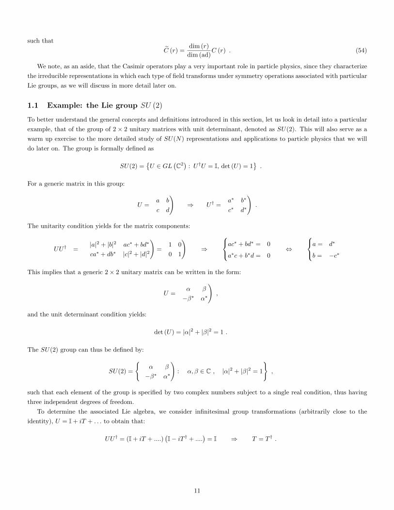
• Vectors (1/2, 1/2):

This coincides with the fundamental representation of the Lorentz group, with:

ΛV (M) = esiKi+t

iJi , si, ti ∈ R (140)

denoting 4-dimensional matrices acting on 4-vectors:

Aµ(x)→ ΛV (M)µνAν(x) , (141)

for which a particular case is Aµ = xµ. It is common to denote the left- and right-handed spinor indices in the form:

ψLa → ΛL(M) ba ψLb ,

ψRa → ΛR(M) ba ψRb . (142)

The vectorial representation thus carries both a left-handed and a right-handed index, and can be equivalently

expressed in spinor form as:

Aaa = σµaaAµ(x) (143)

Note that since ΛL(M) = M and ΛR(M) = M∗ (up to the equivalency established above), a Lorentz vector in spinor

form transforms as:

Aaa →M ba (M∗) b

a Abb = M ba (M∗) b

a σµ

bbAµ = (MσµM

†)aaAµ = (σµ)aaΛV (M)µνA

ν , (144)

using the map between the SL(2,C) and Lorentz groups, so we see that the vector transformation defined above is

equivalent to the spinor transformation laws.

• Tensors:(12 ,

12

)⊗(12 ,

12

)

The tensor product of two vector representations of the Lorentz group can be obtained from the tensor product of

spin-1/2 representations of SU(2):

(1

2,

1

2

)⊗(

1

2,

1

2

)=

(1

2⊗ 1

2,

1

2⊗ 1

2

)

= (0⊕ 1, 0⊕ 1)

= (0, 0)⊕ (1, 1)⊕ (0, 1)⊕ (1, 0) , (145)

where the first two terms correspond to the symmetric part of the tensor product and the last two terms correspond

to the anti-symmetric part. The latter, in particular, corresponds to an anti-symmetric Lorentz tensor with two

vector indices:

Fµν = −Fνµ . (146)

We may define the dual tensor:

Fµν =1

2εµνρσF

ρσ , (147)

26

from which we may define:

F±µν =1

2

(Fµν ± Fµν

), (148)

such that Fµν = F+µν + F−µν . It is easy to check that F±µν = ±F±µν . We thus obtain a decomposition of the anti-

symmetric tensor in terms of a self-dual and an anti-self dual component. Taking into account that under a

Lorentz transformation:

Fµν → Λ ρµ Λ σ

ν Fρσ , Fµν → Λ ρµ Λ σ

ν Fρσ , (149)

we can see that the self-dual or anti-self dual character of the tensor is preserved under Lorentz transformations, so

that F+µν and F−µν correspond to the (1, 0) e (0, 1) irreducible representations of the Lorentz group.

We note that the Maxwell tensor Fµν = ∂µAν−∂νAµ transforms in this representation, and its components describe

the electric and magnetic fields in terms of the electrostatic potential and the vector potential in terms of the 4-

vector potential Aµ = (φ,A). In this case, the duality transformation exchanges the components of the electric and

magnetic fields Ei ↔ Bi, which constitutes a symmetry of the electromagnetic interactions.

The symmetric part of the tensor product yields a Lorentz scalar in the (0, 0) representation, corresponding to scalar

fields φ that are invariant under Lorentz transformations, and a symmetric and traceless tensor hµν in the (1, 1)

representation. In general relativity, perturbations of the metric about flat Minkowski space of this form correspond

to gravitational waves and to the putative graviton particles that correspond to the latter in the (yet unknown)

quantum formulation of the theory.

2.1.3 Spinor bilinears

Weyl spinors are used to describe spin-1/2 particles and the associated fields that generalize the wavefunction in the

relativistic formulation of quantum mechanics. It is thus useful to discuss some of the Lorentz invariant quantities that we

may construct from spinor fields and which may thus appear in the Lagrangian function that describes such particles. The

most important terms in a Lagrangian are the quadratic terms, which lead to linear terms in the equations of motion via

the Euler-Lagrange equations. These then correspond to kinetic and mass terms for the fields, with the former including

field derivatives.

• Majorana mass term:

ψTLσ2ψL → (ΛL(M)ψL)Tσ2 (ΛL(M)ψL)

→ ψTLΛTL(M)σ2ΛL(M)ψL

→ ψTL(σ2Λ−1L (M)σ2

)σ2ΛL(M)ψL

→ ψTLσ2Λ−1L (M)ΛL(M)ψL

→ ψTLσ2ψL , (150)

where we have used that(Λ−1L

)T= ΛR(M)† = σ2ΛL(M)σ2 as obtained in Eq. (136) and (137). A term of the form

ψTRσ2ψR is also invariant under Lorentz transformations. Mass terms for spin-1/2 left-handed or right-handed fields

can be constructed with Majorana terms of this form provided that they are allowed by other symmetries.

27

• Dirac mass term:

χ†LψR → (ΛL(M)χL)†

(ΛR(M)ψR)

→ χ†LΛ†L(M)ΛR(M)ψR

→ χ†LΛ−1R (M)ΛR(M)ψL

→ χ†LψR . (151)

A term of the form χ†RψL is also Lorentz invariant for similar reasons. Note that Dirac mass terms combine the

left- and right-handed parts of a Dirac spinor, which are given by distinct Weyl spinors, while the Majorana terms

combine spinors in the same Weyl representation. In the Standard Model, as we will see later, the masses of the

spin-1/2 charged leptons and quarks corresponds exclusively to Dirac mass terms, while the neutrino masses may

possibly have a contribution from Majorana terms.

• Weyl currents:

jLµ = χ†LσµψL → (ΛL(M)χL)†σµ (ΛL(M)ψL)

→ χ†LΛ†L(M)σµΛL(M)ψL

→ χ†LM†σµMψL

→ χ†LσνΛνµψL

→ ΛνµjLν . (152)

Thus the left-handed Weyl current jLµ transforms as a Lorentz vector, the same occurring for the analogous right-

handed Weyl current jRµ involving right-handed spinors. To obtain Lorentz invariant quantities, we may contract

these currents with other vectors in a Lorentz invariant way. For example, the fermion kinetic term given by:

χ†L,Rσµ∂µψL,R (153)

is a Lorentz scalar since:

∂µ =∂

∂xµ→ ∂

∂x′µ=

∂xν

∂x′µ∂

∂xν=(Λ−1

)νµ∂ν . (154)

In a similar way, we can couple the fermionic current to the electromagnetic potential in a Lorentz invariant way,

such that jL,Rµ describes the electric current associated with a charged fermion:

ηµνjµL,RA

ν → ηµνΛµαΛνβjαL,RA

β = ηαβjαL,RA

β . (155)

2.1.4 Parity and charge conjugation

The parity operator acts on the Lorentz group generators in the adjoint representation as:

P JiP−1 = Ji , P KiP

−1 = −Ki , (156)

as one can check by explicitly constructing the matrices associated to the generators. Hence, the angular momentum

operators Ji, which generate spatial rotations, are pseudo-vectors that remain invariant under spatial reflections, while

the boost generators Ki are normal vectors that change direction under parity transformations. From this we may also

28

conclude that:

PJ±i P−1 =

1

2P(Ji ± iKi

)P−1 = J∓i , (157)

such that a parity transformation exchanges the left- and right-handed representations.

Charge conjugation, which exchanges particles and the corresponding anti-particles, has similar consequences. For

example, for a right-handed Weyl spinor ψR we may define the conjugate spinor as:

ψcR ≡ σ2ψ∗R , (158)

such that under a Lorentz transformation:

ψcR → σ2ΛR(M)∗ψ∗R

→ σ2σ2ΛL(M)σ2ψ∗R

→ ΛL(M)ψcR . (159)

Hence, the conjugate of a right-handed spinor is a left-handed spinor and, analogously, the conjugate of a left-handed

spinor χcL = σ2χ∗L transforms in the right-handed representation.

2.2 Poincare group

The transformations of the Poincare group include both Lorentz transformations and space-time translations, forming the

group:

P ={

(Λ, a) : Λ ∈ L, a ∈ R4}, (160)

such that the action of the group elements in a coordinate system is given by:

xµ → x′µ = Λµνxν + aµ . (161)

The group multiplication law is given by:

(Λ1, a1).(Λ2, a2)x = (Λ1, a1).(Λ2x+ a2) = Λ1(Λ2x+ a2) + a1 = Λ1Λ2x+ Λ1a2 + a1

= (Λ1Λ2,Λ1a2 + a1)x . (162)

The identity element is naturally e = (I4, 0) and for each group element we have the inverse element:

(Λ, a)−1 = (Λ−1,−Λ−1a) , (163)

since

(Λ, a)−1.(Λ, a) = (Λ−1,−Λ−1a).(Λ, a) = (Λ−1Λ,Λ−1a− Λ−1a) = (I4, 0) = e . (164)

29

As should be familiar in quantum mechanics, spatial translations are generated by the linear momentum operator, while

the Hamiltonian generates time translations:

Ψ(x + ε, t+ τ) = Ψ(x, t) + iε · (−i∇Ψ(x, t))− iτ(i∂Ψ(x, t)

∂t

)

= Ψ(x, t) + iε · PΨ(x, t)− iτHΨ(x, t) , (165)

for infinitesimal translations ε and τ in space and time, respectively. We can assemble these two operators in the 4-

momentum relativistic operator generating space-time translations:

Pµ = −i∂µ . (166)

The Lorentz group generators that we have determined earlier also admit a representation in terms of differential operators:

Mµν = −i(xµ∂ν − xν∂µ) , (167)

satisfying the commutation relations:

[Mµν , Mµν ] = i(ηµβMνα + ηµαMβν + ηνβMαµ + ηναMµβ

), (168)

which, apart from a factor of i, are the same commutators as for the σµν generators in Eq. (129). We can also easily check

that:

[Mµν , Pρ] = i(ηνρPµ − ηµρPν

)= i (σµν)

σρ Pσ , [Pµ, Pν ] = 0 . (169)

The Poincare algebra is thus given by:

L(P) = span(Pµ, Mµν) . (170)

We note that, as previously defined:

Ji =1

2εijkMjk = εijkxjPk (171)

are the angular momentum operators generating spatial rotations, while Ki = M0i are the boost generators.

An important quantity to define is the Pauli-Lubanski vector:

Wµ =1

2εµνρσM

νρPσ , (172)

with the following properties:

WµPµ = 0 , (173)[

Wµ, Pν

]= 0 ,

[Wµ, Mαβ

]= −i

(ηµβWα − ηµαWβ

),

[Wµ, Wα

]= −iεµαβνW βP ν , (174)

30

The Lorentz invariant quadratic operators:

P 2 = PµPµ , W 2 = WµW

µ , (175)

commute with all the generators of the Poincare group, thus constituting the Casimir operators of the Poincare group and

from which we can label the different irreducible representations. We may write, in particular:

W 2 =1

4εµνρσε

µαβγM

νρPσMαβP γ

=1

4[−ηνα(ηρβησγ − ηργησβ)− ηνβ(ηργησα − ηραησγ)− ηνγ(ηραησβ − ηρβησα)] MνρPσMαβP γ

= −1

2MαβPγM

αβP γ + MαγPβMαβP γ

= −1

2MαβM

αβP 2 + MαγMαβPβP

γ , (176)

where we used the form of the contraction of two Levi-Civita tensors and the commutation relations (169).

As we know from the theory of Special Relativity, the Casimir opertor P 2 = −m2 for a particle of mass m, so that

different irreducible representations of the Poincare group will correspond to particles with different mass. We also have

that the state of a particle with mass m and 4-momentum p is an eigenstate of the Pµ generator:

Pµ|m, p, σ〉 = pµ|m, p, σ〉 (177)

where we have denoted by σ any other quantities that characterize the state in a given representation and that we wish

to determine. Under a Lorentz transformation in a given representation R(Λ, 0) we obtain a state with 4-momentum Λp:

R(Λ, 0)|m, p, σ〉 = |m,Λp, σ〉 . (178)

Let us check that this is also an eigenstate of Pµ. First, let us note that Pµ, being a group generator, transforms in the

adjoint representation and is a Lorentz vector:

R(Λ, 0)PµR−1(Λ, 0) = Λ ν

µ Pν . (179)

Thus,

Pµ (R(Λ, 0)|m, p, σ〉) = R(Λ, 0)R−1(Λ, 0)PµR(Λ, 0)|m, p, σ〉= R(Λ, 0)Λ ν

µ Pν |m, p, σ〉= Λ ν

µ pνR(Λ, 0)|m, p, σ〉= (Λp)µ|m,Λp, σ〉 . (180)

This means that, in constructing the states in the different representations of the Poincare group, we may take as reference

state a state with a given momentum, such that states with an arbitrary momentum can be obtained from this reference

state by performing a Lorentz transformation. The choice of this reference momentum will be different for particles with

and without mass, such that we must analyze these two cases separately.

31

2.2.1 Massive representations

For states of a massive particle, m 6= 0, we may take as reference the 4-momentum in the particle’s rest frame, pµ = (m,0).

This choice is obviously invariant under spatial rotations, i.e the states:

R(O, 0)|m, (m,0), σ〉 , O ∈ SO(3) , (181)

are also eigenstates of Pµ with momentum eigenvalue pµ = (m,0). We may thus obtain the irreducible representations for

massive particles from the irreducible representations of SO(3) ∼= SU(2), since the generators of the two groups satisfy

the same algebra. Note, in particular, that the fundamental representation of the SO(3) Lie algebra, corresponding to the

anti-symmetric 3× 3 matrices, coincides with the adjoint representation of the SU(2) algebra obtained in Eq. (59). As we

have seen, SU(2) irreducible representations are labelled by their spin and its component along the z axis, which to avoid

confusion with the particle’s mass we may write as j3 = −j, . . . , j. We thus have σ = (j, j3) and:

R(O, 0)|m, (m,0), j, j3〉 = R(j)j3,j′3

(O)|m, (m,0), j, j′3〉 , (182)

where R(j)j3,j′3

(O) are the rotation matrices in a spin-j representation. The SO(3) group is designated as the Little Group

for massive representations of the Poincare group, i.e. the sub-group that preserves the form of the states with 4-momentum

pµ = (m,0).

For these states, the components of the Pauli-Lubanski vector are given by:

W0|m, (m,0), j, j3〉 =1

2ε0ijkM

ijP k|m, (m,0), j, j3〉 = 0 ,

Wi|m, (m,0), j, j3〉 =1

2εijk0M

jkP 0|m, (m,0), j, j3〉 = −mJi|m, (m,0), j, j3〉 , (183)

and thus the Casimir operator W 2 is given by:

W 2|m, (m,0), j, j3〉 = m2J2|m, (m,0), j, j3〉 = m2j(j + 1)|m, (m,0), j, j3〉 . (184)

Hence, we see that the irreducible representations of the Poincare group correspond to particles with different mass and

spin for the case m 6= 0.

2.2.2 Massless representations

In the case m = 0, there is no rest frame for the particle to use as reference 4-momentum, but we could e.g. choose

kµ = E(1, 0, 0, 1), where E denotes the particle’s energy. This form of the 4-momentum is preserved by the isometries of

the Euclidean (x, y) plane, which include rotations about the z axis and translations along x and y. These form the group

ISO(2), which thus constitutes the Little Group for m = 0.

Let us denote the states with 4-momentum kµ as |k, σ〉, such that the components of the Pauli-Lubanski vector are:

W0|k, σ〉 =1

2ε0ij3M

ijP 3|k, σ〉 = EM12|k, σ〉 = EJ3|k, σ〉 ,

W3|k, σ〉 =1

2ε3ij0M

ijP 0|k, σ〉 = −EM12|k, σ〉 = −EJ3|k, σ〉 ,

W1|k, σ〉 =

(1

2ε1ij0M

ijP 0 + ε1023M02P 3

)|k, σ〉 = −E

(M23 + M02

)|k, σ〉 = −E

(J1 + K2

)|k, σ〉 ,

W2|k, σ〉 =

(1

2ε2ij0M

ijP 0 + ε2013M01P 3

)|k, σ〉 = −E

(M31 − M01

)|k, σ〉 = −E

(J2 − K1

)|k, σ〉 . (185)

32

The relevant operators are, thus,{J3, S1, S2

}, where Si ≡ Wi, such that with (122) we obtain the algebra:

[S1, S2] = 0 , [J3, S1] = iS2 , [J3, S2] = −iS1 . (186)

Note that this is also the algebra satisfied by the linear momentum operators on the (x, y)-plane, identifying Si ↔ Pi,

i = 1, 2, along with the z component of the angular momentum, which thus constitutes the algebra of ISO(2). It is easy

to check that, defining S = (S1, S2),

[S2, Si] = [S2, J3] = 0 , (187)

such that S2 commutes with all the generators of the Little Group and is therefore the non-trivial Casimir operator for

massless representations. We may then define the Weyl-Cartan basis for the Little Group ISO(2) with J3 yielding the

only element in the Cartan sub-algebra and the ladder operators:

S± = S1 ± iS2 (188)

such that:

[J3, S±] = ±S± . (189)

We may then obtain the states in massless particle representations in a similar way to the irreducible representations of

SU(2), with:

S2|k, s, j3〉 = s2|k, s, j3〉 ,J3|k, s, j3〉 = j3|k, s, j3〉 ,

J3

(S±|k, s, j3〉

)=

(S±J3 ± S±

)|k, s, j3〉 = (j3 ± 1) S±|k, s, j3〉 , (190)

which means that S±|k, s, j3〉 ∝ |k, s, j3 ± 1〉. However, note that:

〈k, s, j3|S2|k, s, j3〉 = 〈k, s, j3|S†±S±|k, s, j3〉 = ||S±|k, s, j3〉||2 = s2 ‖|k, s, j3〉‖2 . (191)

This means that S±|k, s, j3〉 = 0 only for s = 0. Therefore, for s 6= 0 there is an infinite set of states, which do not find

any realization in nature. The only physical states are those with s = 0, characterized uniquely by the eigenvalues of J3

and which we may thus denote as |k, j3〉, such that:

S±|k, , j3〉 = 0 . (192)

Given our choice for the reference 4-momentum, we see that J3 is the component of the particle’s spin in the direction

of its 3-momentum, and its eigenvalues are denoted as the helicity of a particle. Note that we obtain the same result

whatever the form of the reference 4-momentum that we had chosen, with kµkµ = 0, so that helicity is Lorentz invariant

for massless particles. For example, massless spin-1/2 particles are described by Weyl spinors, with h ≡ j3 = +1/2 for

right-handed spinors and h = −1/2 for left-handed spinors, which are thus irreducible representations of the Lorentz and

Poincare groups.

33

3 SU(N) groups

The unitary and special unitary groups also play a special role in particle physics, constituting the basis for the global

and gauge symmetries upon which the Standard Model of particle physics is built. They are defined, respectively, as:

U(N) ={U ∈ GL(CN ) : U†U = IN

}, SU(N) = {U ∈ U(N) : det(U) = 1} . (193)

Note that the unitary condition U†U = IN implies |det(U)|2 = 1, i.e. det(U) = ±1. One can construct a map between

the groups U(1)× SU(N) and U(N) in the following way:

f : U(1)× SU(N)→ U(N)

f(z, U) = zU , z ∈ U(1), U ∈ SU(N) . (194)

Note that U(1) corresponds to the group of complex numbers with unit modulus:

U(1) = {z ∈ C : |z| = 1} . (195)

Let us check that this map is a group homomorphism. First, note that for any unitary matrix U ∈ U(N), we may write:

detU = ζN ⇒ |ζ|N = 1 ⇒ |ζ| = 1 ⇒ ζ ∈ U(1) . (196)

Let us then consider matrices of the form A = ζ−1U , which satisfy:

A†A =(ζ−1U

)† (ζ−1U

)= U†ζζ−1U = U†U = IN ,

det(A) =(ζ−1

)NdetU = (det(U))

−1detU = 1 , (197)

so that A ∈ SU(N). Hence, we have that:

f(ζ, ζ−1U) = ζζ−1U = U , (198)

such that we can obtain any matrix U in U(N) through the map f .

Second, we need to find how many elements of U(1)× SU(N) are mapped to the identity matrix IN :

Ker(f) = {(z,A) ∈ U(1)× SU(N) : f(z,A) = IN} . (199)

Note that, for these elements:

det(zA) = zN det(A) = zN = 1 ⇒ z = e2πinN , n ∈ Z , (200)

such that Ker(f) = ZN . This then implies the following group isomorphism:

U(N) ∼= U(1)× SU(N)/ZN , (201)

i.e. the matrices in SU(N) and U(N) differ only by a complex phase z = eiθ with period 2π/N .

We will then focus on the SU(N) groups, and analogously to what we have already found for SU(2) the Lie algebra

for these groups is given by:

L (SU (N)) ={T ∈M

(CN)

: T = T †, Tr (T ) = 0}. (202)

34

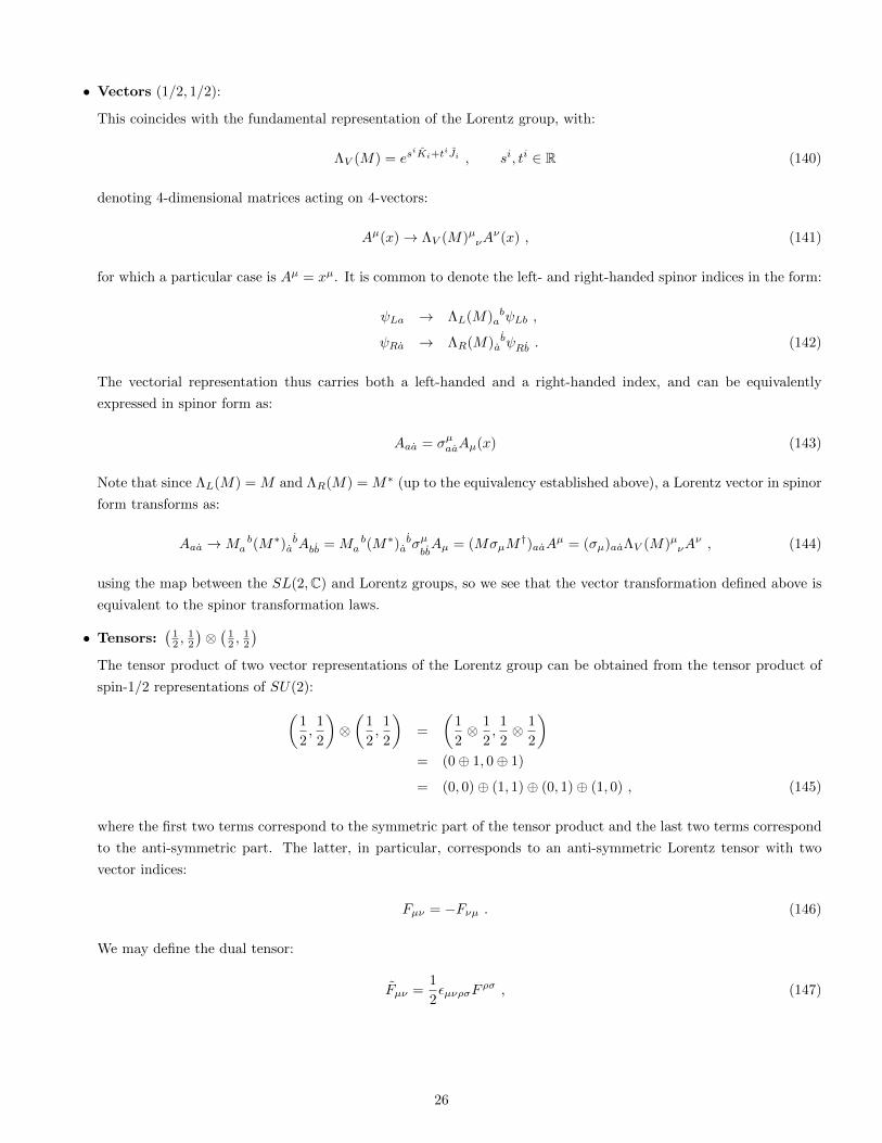
On the 2N2 real degrees of freedom of a complex N ×N matrix, the hermiticity condition imposes N2 constraints, and a

further real constraint is imposed by the tracelessness condition, leaving N2−1 degrees of freedom which is the dimension

of the Lie algebra and of the adjoint representation.

The Cartan sub-algebra of SU(N), corresponding to the maximum number of commuting generators, is trivially given

by the diagonal generators of the Lie algebra. Since there are N distinct real components in a hermitian matrix and the

tracelessness condition allows one to write one of these components in terms of the others, we conclude that this yields

an (N − 1)-dimensional Cartan sub-algebra, i.e. that SU(N) groups have rank N − 1. As we have described in the first

section, we may construct a basis for the Lie algebra and determine its roots and weights from the Cartan sub-algebra

generators, which we will do explicitly for the case of SU(3).

3.1 Irreducible representations of SU(N)

Representations of SU(N) are given in terms of tensor fields that transform under SU(N) in different ways. They are

also represented in terms of their dimension. In particular, we have:

• Fundamental representation

N : ψa → U ba ψb , a, b = 1, . . . , N (203)

where U ∈ SU(N).

• Complex conjugate representation

N : ψa → U∗abψb . (204)

• Tensor representations

Np × Nq

: ψa1...aq

b1...bp→ U∗a1c1 . . . U

∗aqcqU

d1b1

. . . Udp

bpψc1...cq

d1...dp. (205)

There are special tensors that are invariant under SU(N) transformations, in particular the generalized Kronecker

delta and Levi-Civita tensors:

δ ba → U c

a U∗bdδdc = U c

a U∗bc = U ca

(U†) bc

=(UU†

) b

a= δ b

a , (206)

εa1...aN → U b1a1 . . . U bN

aN εb1...bN

→(δ b1a1 + iT b1

a1

). . .(δ bNaN + iT bN

aN

)εb1...bN

→ εa1...aN + iT b1a1 εb1a2...aN + . . .+ iT bN

aN εa1a2...bN

→ εa1...aN + iT a1a1 εa1a2...aN + . . .+ iT aN

aN εa1a2...aN

→ εa1...aN (1 + iTr(T ))

→ εa1...aN , (207)

and analogously for εa1...aN . An equivalent way of proving the invariance of the Levi-Civita tensor is to note that:

U b1a1 . . . U bN

aN εb1...bN = det(U)εa1...aN , (208)

35

such that for an SU(N) matrix with unit determinant the invariance of the Levi-Civita tensor follows trivially.

These tensors can be used to construct new tensors, for example:

ψa1...apa1...ap → U∗a1c1 . . . U∗ap

cpUd1

a1 . . . U dpap ψ

c1...cpd1...dp

→(UTd1a1U

∗a1c1

). . .(UTdp

apU∗ap

cp

)ψc1...cp

d1...dp

→ δd1c1 . . . δdpcpψc1...cp

d1...dp

→ ψa1...apa1...ap , (209)

where we used that UTU∗ = (U†U)∗ = I. Similarly, another invariant under SU(N) is:

εa1...aNψa1...aN → εa1...aNU b1a1 . . . U bN

aN ψb1...bN = εb1...bNψb1...bN . (210)

The complex conjugate representation can also be obtained as a contraction of the Levi-Civita tensor and a tensor

representation with fundamental (lower) indices:

ψa = εab1...bN−1χb1...bN−1→ εab1...bN−1U c1

b1. . . U

cN−1

bN−1χc1...cN−1

→ εed1...dN−1U∗aeU∗b1d1. . . U

∗bN−1

dN−1U c1b1

. . . UcN−1

bN−1χc1...cN−1

→ U∗aeεed1...dN−1

(U†U

) c1

d1. . .(U†U

) cN−1

dN−1χc1...cN−1

→ U∗aeεed1...dN−1χd1...dN−1

→ U∗aeψe . (211)

Hence, we see that the free indices, i.e. those that are not summed over, determine the transformation law for a given

tensor. Tensors with no free indices will be invariant under SU(N) transformations.

We would like to determine the irreducible representations within such tensorial products. For this, let us focus on

representations with only lower indices, since as we have seen indices can be raised with the Levi-Civita tensor.

Let us consider first the 2-index tensor ψab, which we may decompose into its symmetric and anti-symmetric parts:

ψab = ψ+ab + ψ−ab , ψ±ab ≡

1

2(ψab ± ψba) . (212)

Under SU(N) transformations:

ψ±ab → ψab = U ca U d

b ψ±cd = U d

a U cb ψ±dc = ±U d

a U cb ψ±cd = ±ψba , (213)

so that (anti-)symmetric tensors are transformed into (anti-)symmetric tensors, and they form invariant sub-spaces. Hence,

ψab is a reducible representation, while ψ±ab are irreducible representations.

In general, the irreducible representations of SU(N) are in a one-to-one correspondence with the irreducible represen-

tations of the permutation group, i.e. a tensor with p indices can be decomposed into irreducible representations of Sp.

In the 2-index tensor example above, the permutations of the two indices a and b yield two irreducible representations

corresponding to the symmetric and anti-symmetric parts.

The irreducible representations of the permutation group can be mapped into the so-called Young tableaux, and

this is also one of the most useful descriptions of the SU(N) irreducible representations. Let us consider an SU(N) tensor

with p indices ψa1...ap and numbers:

p1 ≥ p2 ≥ . . . ≥ ps ,s∑

i=1

pi = p . (214)

36

We can then construct the following Young tableau, associated with the tensor ψa1...ap1ap1+1...ap1+p2...ap , with p1 boxes in

the first line, p2 boxes in the second, etc:

ap1+p2ap1+1

a1 a2 ap1

ap

. . .

. . .

...

This tableau is:

• symmetric in the indices appearing in the same line of the tableau;

• anti-symmetric in the indices appearing in the same column of the tableau.

THEOREM: Young tableaux with a number of lines smaller or equal to N are in a one-to-one correspondence with

the irreducible representations of SU(N).

To compute the dimension of a representation from the associated Young tableau, we need to consider standard

tableaux, which correspond to inserting the indices 1, . . . , N in the boxes of Young tableaux such that:

• indices do not decrease from left to right within each row;

• indices increase from top to bottom in each column.

The number of standard tableaux that we can construct then yields the dimension of the representation. The following

table illustrates the Young tableaux and the standard tableaux associated with the simplest representations.

Representation Tensor Young tableau Standard tableaux Dimension

Fundamental

Symmetric

Anti-symmetric

Symmetric

Anti-symmetric

N

N × N

N × N

Nk

Nk

ψa

ψ(ab)

ψ[ab]

ψ(a1...ak)

ψ[a1...ak]

1 N. . . N

. . .

. . .

1 1 1 N

2 2

1

2N(N + 1)

. . .12

1N

1

2N(N − 1)

. . .

. . .

. . .

1 1

1 2

...

�N + k + 1

k

�

...

...

.... . .1

k

�Nk

�

37

Consider, for example, the case of SU(3), for which the symmetric and anti-symmetric representations are given by:

1 1 1 2

1 3 2 2

2 3 3 3

1 2

1 3

2 3

3 =

6 =

Notice that the anti-symmetric representation in SU(3) corresponds to the complex conjugate representation, also

denoted as anti-fundamental representation, since we can write ψa = εabcψbc. The adjoint representation of SU(3),

which has the dimension of the Lie algebra, 32 − 1 = 8, is given by the following Young tableau:

1 1 2

1 1 3

1 2 2

1 2 3

1 3 2

1 3 3

2 2 3

2 3 3

8 =a b

c

This corresponds to a tensor symmetric in the a and b indices and anti-symmetric in the a and c indices, which can be

written as the following combination of permutations of the 3-index tensor:

1

4(ψabc + ψbac − ψcba − ψbca) . (215)

Young tableaux are particularly useful in decomposing tensor products of two SU(N) representations into a sum of

irreducible representations. To do this, we start by writing the labels a, b, c, . . . in the boxes of the Young tableau of the

first representation, with a symbols in the first row, b symbols in the second row, etc, as illustrated in the figure below:

a a a a

b b b

c c

We then attach the boxes of the first diagram to the second diagram, starting with the boxes with a label and then the

boxes with b label, etc, such that we get new Young tableaux where equal labels cannot appear in the same column. In

addition, for each new Young tableau that we obtain with this procedure, we must read all the labels from right to left in the

first row and then in the second row, etc. This yields a sequence of labels for each new tableau where, to the left of each label,

the number of b labels cannot exceed the number of a labels, the number of c labels cannot exceed the number of b labels,

etc. This means, for example, that sequences aab and aba are allowed, while abba is not allowed.

38

This procedure is best understood by considering a few examples, so let us consider the products of the lowest dimension

irreducible representations in SU(3):

× = +a a

a

3 × 3 = 6 + 3

3 × 3 = 1 + 8

× =a

a

+ a

× = +a a

a

3 × 6 = 10 + 8

× =

8 × 8 = 27 + 10 + 10 + 8 + 8 + 1

a a

b

a a

b

a a

b

a

a b

a

a

b

a

a

b a b

a

+

+

+

+

Note that in SU(3) a column with 3 boxes corresponds to the singlet representation 1, i.e. an invariant tensor, since

there is only one standard tableau with numbers (1, 2, 3). This means that in determining the dimension of a representation

we may ignore all columns with 3 boxes. The same holds for columns with N boxes in a general SU(N) representation.

Also note that in the last example above there are two representations with dimension 10, which we have labeled as 10

and 10, so that they are complex conjugate. Which one is the conjugate representation, denoted with a bar, is a matter of

convention, but looking at the corresponding Young tableaux one sees that, putting them together, one obtains a tableau

with three rows (ignoring the singlet column as explained above). The same holds for 3 and 3. This is actually a generic

feature of complex conjugate representations: for each SU(N) representation, its complex conjugate can be obtained by

looking at the completion of its Young tableau that yields N rows and the same number of columns, as illustrated below.

For the example of SU(3) above, we can clearly see that the complex conjugate of the adjoint representation is the adjoint

representation itself, and this is true for all SU(N) - the adjoint representation is said to be a real representation.

39

3.2 SU(3) and the quark model

SU(N) groups play an important role in particle physics, being the basis for the gauge theories on which the Standard

Model is built. The first and simplest application of these groups, other than SU(2) for the spin of elementary particles

as we have already discussed, is the quark model to describe the meson and baryon particles in terms of elementary

constituents, known as the quarks. The lightest mesons and baryons can be described in terms of three elementary quarks,

known as up, down and strange, although now we know that there are actually six quark “flavours” with the addition of

the charm, bottom and top quarks. The similarity between the masses of certain groups of mesons and baryons suggests

an underlying symmetry between the quark constituents, and for the case of the three lightest quarks this is naturally

SU(3) as we will now describe in more detail.

The main idea is that the three lightest elementary quarks are related by SU(3) transformations, forming a vector

space that transforms in the fundamental representation of this group. Their corresponding anti-particles then naturally

transform in the anti-fundamental (or complex conjugate) representation, and composite states as mesons and baryons

transform in tensor products of these representations, which as we have seen above can be decomposed into irreducible

representations. Mesons and baryons in the same irreducible representation of SU(3) should have equal masses since

they should be related by SU(3) transformations, but actually their masses are slightly different due to the fact that the

elementary quarks themselves have different masses and charges. Note that the mass, i.e. the rest energy, of a composite

state depends not only on the mass of its constituents but also on their interaction energy, which include in the case of

quarks their strong, weak and electromagnetic interactions. Hence, the SU(3) flavour symmetry, and its generalization to

SU(6) when including all the known elementary quarks, is only an approximate symmetry, which nevertheless explains

very well the spectrum of meson and baryon masses.

Let us start by discussing the SU(3) Lie algebra, which corresponds to the hermitian traceless 3 × 3 matrices. The

most widely used basis for this algebra is given by the Gell-Mann matrices, after Murray Gell-Mann who, along with

George Zweig, independently proposed the quark model, also known as the “Eightfold way”, in 1964. These are given by:

λ1 =

0 1 0

1 0 0

0 0 0

, λ2 =

0 −i 0

i 0 0

0 0 0

, λ3 =

1 0 0

0 −1 0

0 0 0

, λ4 =

0 0 1

0 0 0

1 0 0

,

λ5 =

0 0 −i0 0 0

i 0 0

, λ6 =

0 0 0

0 0 1

0 1 0

, λ7 =

0 0 0

0 0 −i0 i 0

, λ8 =

1√3

1 0 0

0 1 0

0 0 −2

. (216)

One can naturally see in these matrices the structure found in the Pauli matrices, and in fact there are three SU(2)

sub-algebras in SU3):

SU(2)I = span {λ1, λ2, λ3} , SU(2)V = span

{λ4, λ5,

λ3 +√

3λ82

}, SU(2)U = span

{λ6, λ7,

√3λ8 − λ3

2

}.(217)

The Gell-Mann matrices satisfy Tr(λiλj) = 2δij and conventionally we choose the basis Ti = λi/2, such that:

Tr(TiTj) =1

2δij , (218)

as we have used for SU(2) as well. There are two diagonal generators in the rank-2 SU(3) algebra, and the Cartan

sub-algebra can be chosen as:

H (SU(3)) = span

{T3, Y =

2√3T8

}, (219)

40

where T3 is known as the isospin generator and Y as the hypercharge generator. We also define:

Q ≡ T3 +Y

2, (220)

which as we will see below corresponds to the electric charge of the quarks.

To complete the Weyl-Cartan basis for SU(3), we define the ladder operators:

T± = T1 ± iT2 , V± = T4 ± iT5 , U± = T6 ± iT7 , (221)

which satisfy the following commutation relations with the diagonal generators of the Cartan sub-algebra:

[T3, T±] = ±T± , [T3, V±] = ± 12V± , [T3, U±] = ∓1

2U± ,

[Y, T±] = ±0 , [Y, V±] = ±V± , [Y, U±] = ±U± . (222)

From these we can immediately infer the roots of the SU(3) Lie algebra:

α(T±) = (±1, 0) , α(V±) = (±1/2,±1) , α(U±) = (∓1/2,±1) . (223)

This means that T± raise/lower the isospin of states in a representation by one unit, while V± and V± either raise or lower

the isospin by 1/2. While T± do not change the hypercharge of a state, both V± and U± change the hypercharge by ±1.

This is illustrated in the following root diagram:

T+T-

V+

V-

U+

U-

-1 -1

2

1

21

T3

-1

-1

2

1

2

1

Y

Note that the root diagram for SU(2) would be 1-dimensional, corresponding e.g. to the pair (T+, T−).

The fundamental representation of SU(3), 3, in the quark model has a basis of states |u〉, |d〉 and |s〉 corresponding

to the the up, down and strange quarks, respectively. These correspond to the basis of vectors (1, 0, 0)T , (0, 1, 0)T and

(0, 0, 1)T . The generators in this representation are given by the Ti normalized Gell-Mann matrices defined above, and

the Cartan sub-algebra is given by:

T3 = diag(1/2,−1/2, 0) , Y = diag(1/3, 1/3,−2/3) , (224)

which implies that the up and down quarks form an isospin doublet, while the strange quark is an isospin singlet. While

u and s have hypercharge 1/3, the d quark has hypercharge −2/3. This yields:

Q = diag(2/3,−1/3,−1/3) , (225)

41

so that the up quark has a +2/3 electric charge, while the down and strange quarks have charge −1/3. The weights of

the fundamental representation are then:

λ(u) = (1/2, 1/3) , λ(d) = (−1/2, 1/3) , λ(s) = (0,−2/3) , (226)

as illustrated in the weight diagram below.

ud

s

-1-

1

2

1

21

T3

-1

-

1

2

1

2

1

Y

It should be clear in this figure that the ladder operators can be used to obtain different states in this representation.

In particular, the T± generators exchange u ↔ d, the V± generators exchange u ↔ s and the U± generators exchange

d↔ s.

The complex conjugate representation 3 has a basis of states |u〉, |d〉 and |s〉, corresponding to the anti-quark

states. Recalling that U = eiT , we have U∗ = e−iT∗, so that the generators in the 3 representation are T i = −T ∗i . In

particular, in the Cartan sub-algebra we have:

T3 = diag(−1/2, 1/2, 0) , Y = diag(−1/3,−1/3, 2/3) , Q = diag(−2/3, 1/3, 1/3) , (227)

so that the anti-quarks have opposite electric charge to the corresponding quarks. The weights in this representation are:

λ(u) = (−1/2,−1/3) , λ(d) = (1/2,−1/3) , λ(s) = (0, 2/3) , (228)

and the weight diagram is given by:

u d

s

-1-

1

2

1

21

T3

-1

-

1

2

1

2

1

Y

42

We can now look at composite states, generically known as hadrons. The simplest states are the mesons, which are

spin-0 bound states of a quark and an anti-quark. Note that quarks are spin-1/2 fermions, corresponding to Dirac spinors.

This means that the quark and anti-quark in a given meson must have opposite spins. In terms of SU(3), mesons must

lie in the tensor product representation 3 × 3 = 8 + 1 as we have obtained above. We hence expect to find an octet of

mesons with similar masses, transforming in the adjoint representation, and an additional SU(3) singlet meson.

As we have discussed in the first section, the weights in a tensor product representation correspond to the sum of the

weights in the individual representations. We then have the following basis of states in the 3× 3 representation:

States Weights

|uu〉, |dd〉, |ss〉 (0, 0)

|ud〉 (1, 0)

|us〉 (1/2, 1)

|du〉 (−1, 0)

|ds〉 (−1/2, 1)

|su〉 (−1/2,−1)

|sd〉 (1/2,−1)

The associated weight diagram is illustrated below, including the names given to the corresponding mesons. Note that

the electric charge of each meson, being a linear combination of the weights, is also the sum of the electric charges of its

quark and anti-quark constituents.

K0= ds K+

= us

Π-

= du

K-= su K

0= sd

Π+

= udΠ0

Η0

Η'-1 -1

2

1

21

T3

-1

-1

2

1

2

1

Y

As one can see, there are three degenerate states with (0, 0) weight, corresponding to |uu〉, |dd〉 and |ss〉, but only

two linear combinations of these states belong to the meson octet, while the remaining must correspond to the singlet

meson. To determine which states are in the octet, we note that such states should be obtained from the remainder

states in the octet by applying SU(3) transformations. Since this can be achieved using the ladder operators, we may,

for example, determine T−|ud〉 and U−|ds〉. Note that these generators take the following form in the fundamental and

anti-fundamental representations:

T− = T1 − iT2 =

0 0 0

1 0 0

0 0 0

, T− = −T1 − iT2 =

0 −1 0

0 0 0

0 0 0

,

U− = T6 − iT7 =

0 0 0

0 0 0

0 1 0

, U− = −T6 − iT7 =

0 0 0

0 0 −1

0 0 0

, (229)

43

such that:

T−|ud〉 = (T−|u〉)⊗ |d〉+ |u〉 ⊗ (T−|d〉) = |dd〉 − |uu〉 ,U−|ds〉 = (U−|d〉)⊗ |s〉+ |d〉 ⊗ (U−|s〉) = |ss〉 − |dd〉 . (230)

These states are not, however, orthogonal, but we can choose the following orthogonal linear combinations:

|π0〉 =1√2

(|uu〉 − |dd〉

), |η0〉 =

1√6

(|uu〉+ |dd〉 − 2|ss〉

), (231)

which thus yield the two (0, 0) mesons in the octet. The singlet meson must be a linear combination of |uu〉, |dd〉 and |ss〉that is orthogonal to both |π0〉 and |η0〉, yielding:

|η′〉 =1√3

(|uu〉+ |dd〉+ |ss〉

), (232)

and it is easy to see that this state remains invariant under SU(3) transformations. i.e. under the exchange of any pair of

quarks.

The other quark bound states occurring in Nature are the baryons, which are composed of 3 quarks, with the

corresponding anti-baryons having 3 anti-quarks. Baryons must then transform in the tensor representation:

3× 3× 3 = (6 + 3)× 3 = 6× 3 + 3× 3 = 10 + 8 + 8 + 1 , (233)

where we have used the SU(3) tensor products obtained earlier using Young tableaux. Not all of these irreducible

representations occur in Nature, since quarks are spin-1/2 fermions that also carry an additional SU(3) “colour” charge,

which is distinct from the SU(3) flavour symmetry that we are considering. Due to Pauli’s exclusion principle, the total

wavefunction of a composite fermionic state must be anti-symmetric under the exchange of any two identical fermions, so

that they cannot simultaneously be in the same state. This singles out the representations 10 and only one of the adjoint

8 representations obtained above. The baryon decuplet includes the spin-3/2 baryons, while the baryon octet contains

the states with total spin 1/2.

Although we will not study in detail the states in these representations, one should note that the most important

baryons are the proton and the neutron, which have spin-1/2. These are the most stable of the baryons, since the others

are short-lived and can decay into other baryons and mesons. The proton is a uud state with weight vector (1/2, 1), and

is thought to be completely stable, while the neutron is a udd state with weight vector (−1/2, 1), and is only stable when

forming bound states with other neutrons and protons inside atomic nuclei. The electric charge of the proton is then +1,

while the neutron has zero electric charge according to our definition of Q.

3.3 Branching SU(3) representations into SU(2) representations

A common feature to SU(N) groups and also other Lie groups used in particle physics is that they include lower rank

sub-groups, and it is useful to understand how the representations of the sub-group are embedded into the larger SU(N)

representations. We will consider the example of SU(3), which as we have seen above includes the group SU(2) in three

possible ways. The simplest possibility is SU(2)I , which corresponds to the sub-group:

U =

(U2 0

0 1

)∈ SU(3) , (234)

where the 2× 2 matrix U2 ∈ SU(2). It is clear that this embedding leaves the strange quark invariant, while performing

SU(2) transformations in the sub-space spanned by the |u〉 and |d〉 states in the fundamental representation. These then

44

form an SU(2)-isospin doublet, so that we have the decomposition:

3SU(3) → (2 + 1)SU(2)I (235)

Similarly, for the complex conjugate representation:

3SU(3) → (2 + 1)SU(2)I (236)

where we recall that the fundamental 2 and complex conjugate 2 representations of SU(2) are equivalent as we derived

in the first section.

Knowing how the fundamental and anti-fundamental representations of SU(3) branch into SU(2)-isospin representa-

tions then allows us to do the branching of other representations. For the case of mesons, for example, we have:

(3× 3

)SU(3)

= (8 + 1)SU(3) → (2 + 1)× (2 + 1)SU(2)I

→ (2× 2 + 2× 1 + 1× 2 + 1× 1)SU(2)I

→ (3 + 1 + 2 + 2 + 1)SU(2)I. (237)

Since an SU(3) singlet will also be an SU(2)I singlet, we then conclude that the meson octet in the adjoint representation

has the following branching:

8SU(3) → (3 + 2 + 2 + 1)SU(2)I. (238)

Each of these multiplets must have a constant hypercharge Y , since the only diagonal generator leading to matrices of

the form (234) is T3. These then correspond to the mesons along the same horizontal lines in the weight diagram given

earlier:

3 = (π+, π0, π−)Y=0 ,

2 = (K+,K0)Y=1 ,

2 = (K−, K0)Y=−1 ,

1 = (η0)Y=0 . (239)

The pions then form an isospin triplet, which corresponds to the isospin-1 adjoint representation of SU(2)I , while the

kaons form two isospin doublets with opposite hypercharges. That the η0 is an isospin singlet should be clear from its

explicit form in (231), since it is invariant under the exchange of the u and d quarks and of their anti-particles, the same

happening for the SU(3) singlet state η′.

Note that the isospin symmetry is actually a much better symmetry than the full SU(3) flavour symmetry since, while

the up and down quarks have similar masses of a few MeV/c2, the strange quark is significantly heavier, with a mass of

around ∼ 140 MeV/c2. The isospin triplet pions then have similar masses of around 140 MeV/c2, while the remaining

octet mesons with a strange quark have masses around 550 MeV/c2. The η′, which is an SU(3) and isospin singlet, has a

much larger mass of ∼ 956 MeV/c2.

45

4 Problems

1. Consider the following set of 4× 4 matrices:

A1 =

0 0 0 0

0 0 1 0

0 -1 0 0

0 0 0 0

, A2 =

0 0 -1 0

0 0 0 0

1 0 0 0

0 0 0 0

, A3 =

0 -1 0 0

1 0 0 0

0 0 0 0

0 0 0 0

B1 =

0 0 0 -1

0 0 0 0

0 0 0 0

1 0 0 0

, B2 =

0 0 0 0

0 0 0 -1

0 0 0 0

0 1 0 0

, B3 =

0 0 0 0

0 0 0 0

0 0 0 1

0 0 -1 0

a) Justify that these matrices form a basis for the Lie algebra of the group SO(4).

b) Verify, for i = 1 and j = 2, the following commutation relations:

[Ai, Aj ] = εijkAk , [Bi, Bj ] = εijkAk , [Ai, Bj ] = εijkBk

c) Consider now the following linear combinations of generators:

Xi =1

2(Ai +Bi) , Yi =

1

2(Ai −Bi) , i = 1, 2, 3

Show that these span two independent sub-algebras, i.e. two commutting algebras, and indicate the Lie group

to which each of these algebras is associated. Is the Lie algebra of SO(4) semi-simple?

d) Compute the Killing form and the Casimir operator for each of the sub-algebras determined in the previous

question.

Hint: Use the identity εijkεilm = δjlδkm − δjmδkl.

2. The sympletic group Sp(2,R) is defined as the group of 2× 2 matrices:

Sp(2,R) ={S ∈ GL(R2) : STJS = J

}

where

J =

(0 1

-1 0

)

46

a) Explain why these matrices form a group under the usual matrix multiplication rule.

b) Given that λ is one of the eigenvalues of a matrix in this group, determine the other eigenvalue.

c) Justify that the following matrices form a basis for the Lie algebra of Sp(2,R) and determine the associated

non-vanishing structure constants:

T1 =

(0 1

0 0

), T2 =

(0 0

1 0

), T3 =

(1 0

0 -1

).

d) Construct the Weyl-Cartan basis from the matrices given above and plot in the same diagram the weights of

the fundamental representation and the roots of the Lie algebra.

e) Determine the components of the Killing metric in the basis {T1, T2, T3}.

3. Consider the following set of 4× 4 matrices:

Aa =

(0 σa

σa 0 ,

), Ba =

(σa 0

0 −σa ,

), Ca =

(σa 0

0 σa ,

), D =

(0 −iIiI 0 ,

)

where 0 and I denote the zero matrix and the 2 × 2 identity matrix, respectively, and σa, a = 1, 2, 3, are the Pauli

matrices, given by:

σ1 =

(0 1

1 0

), σ2 =

(0 −ii 0

), σ3 =

(1 0

0 -1

)

a) Show that these matrices form a closed Lie algebra.

Hint: Use the relation σaσb = Iδab + iεabcσc.

b) Taking H1 = B3 and H2 = C3 as the generators of the Cartan sub-algebra, determine the weight diagram of

the fundamental representation.

c) Show that the matrices Eα = {A±, D±, F±, G±} ccomplete the Weyl-Cartan basis for this Lie algebra, where:

A± = A1 ± iA2 , D± = A3 ± iD , B± = B1 ± iB2 , C± = C1 ± iC2

F± = B± + C± , G± = B± − C±

and plot the associated root diagram.

47

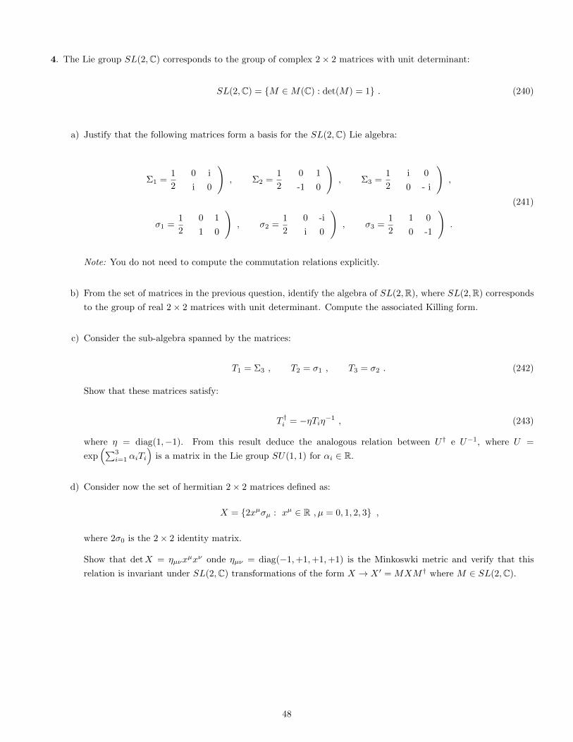
4. The Lie group SL(2,C) corresponds to the group of complex 2× 2 matrices with unit determinant:

SL(2,C) = {M ∈M(C) : det(M) = 1} . (240)

a) Justify that the following matrices form a basis for the SL(2,C) Lie algebra:

Σ1 =1

2

(0 i

i 0

), Σ2 =

1

2

(0 1

-1 0

), Σ3 =

1

2

(i 0

0 - i

),

(241)

σ1 =1

2

(0 1

1 0

), σ2 =

1

2

(0 -i

i 0

), σ3 =

1

2

(1 0

0 -1

).

Note: You do not need to compute the commutation relations explicitly.

b) From the set of matrices in the previous question, identify the algebra of SL(2,R), where SL(2,R) corresponds

to the group of real 2× 2 matrices with unit determinant. Compute the associated Killing form.

c) Consider the sub-algebra spanned by the matrices:

T1 = Σ3 , T2 = σ1 , T3 = σ2 . (242)

Show that these matrices satisfy:

T †i = −ηTiη−1 , (243)

where η = diag(1,−1). From this result deduce the analogous relation between U† e U−1, where U =

exp(∑3

i=1 αiTi

)is a matrix in the Lie group SU(1, 1) for αi ∈ R.

d) Consider now the set of hermitian 2× 2 matrices defined as:

X = {2xµσµ : xµ ∈ R , µ = 0, 1, 2, 3} ,

where 2σ0 is the 2× 2 identity matrix.

Show that detX = ηµνxµxν onde ηµν = diag(−1,+1,+1,+1) is the Minkoswki metric and verify that this

relation is invariant under SL(2,C) transformations of the form X → X ′ = MXM† where M ∈ SL(2,C).

48

5. A Dirac spinor ψ transforms in the (1/2, 0)⊕ (0, 1/2) representation of the Lorentz group and can be written in the

form:

ψ =

(χL

χR

),

where χL is a left-handed Weyl spinor and χR a right-handed Weyl spinor. The transformation matrices in the Dirac

representation are then given by:

ΛD(M) =

(ΛL(M) 0

0 ΛR(M)

),

where M ∈ SL(2,C) such that:

ΛL(M) = e−12 (s

i+iti)σi , ΛR(M) =(ΛL(M)−1

)†,

where si, ti are real parameters and σi are the Pauli matrices.

Define the Dirac gamma matrices as:

γµ =

(0 σµ

σµ 0

),

where σµ = (I2, σi) and σµ = (I2,−σi) = σ2σTµ σ2.

a) Show that for an infinitesimal Lorentz transformation ψ → ψ + δψ one has

δψ = iεµνσµνψ ,

where σµν = i4 [γµ, γν ] and εµν is an infinitesimal anti-symmetric tensor.

b) Show that the spinor bilinear

ψψ ,

where ψ ≡ ψ†γ0, is invariant under finite Lorentz transformations.

c) Using the relation between SL(2,C) and Lorentz group matrices

σµΛµν = M†σνM ,

show that:

ΛD(M)−1γµΛD(M) = Λ νµ γν

d) Use the previous result to determine how the following spinor bilinear:

ψγµψ

transforms under the Lorentz group.

Hint: Use the following relations:

[σi, σj ] = 2iεijkσk , εiklεjkl = 2δij ,

ΛL,R(M)∗ = σ2ΛR,Lσ2 .

49

6. Consider the group SU(3).

a) Verify the following identity for an arbitrary 3× 3 matrix:

U ia U

jb U

kc εijk = det(U)εabc

for a = 1, b = 2 and c = 3. Use this result to show that the Levi-Civita tensor is invariant under SU(3).

Assuming the transformation law for an SU(3) tensor ψab, verify that ψa = εabcψbc transforms in the funda-

mental representation of the group.

b) Using Young tableaux, decompose the following tensor product into irreducible representations of SU(3):

3× 3× 3

For each of the irreducible representations obtained, indicate the symmetry properties of the associated tensor.

c) In the SU(3) quark model, the fundamental representation qi = (u, d, s)T has weights u = (1/2, 1/3), d =

(−1/2, 1/3) and s = (0,−2/3) with respect to the isospin and hypercharge generators (T3, Y ) of the Cartan

sub-algebra.

Determine the weight diagram for the baryon decuplet and write the corresponding normalized states in the

basis |qiqjqk〉.

Hint: Construct the Young tableau associated with the 10 representation of SU(3) to determine the symmetry

properties of the associated states.

d) Show that the trace of the electric charge generator Q = T3 + Y/2 vanishes for the baryon decuplet.

Note: The trace of an operator O in a vector space spanned by states {|ψi〉} is given by:

Tr(O) =∑

i

〈ψi|O|ψi〉

7. Consider the group SU(3).

a) Using Young tableaux, decompose the following tensor products in terms of irreducible representations:

3× 3

8× 3

6× 3

Note that the 6 representation corresponds to the symmetric part of the tensor product 3× 3.

b) In Quantum Chromodynamics (QCD), each quark transforms in the fundamental representation of the group

SU(3)c, forming a “colour” triplet (qr, qg, qb) (for “red”, “green” and “blue”) with weights qr = (1/2, 1/3),

50

qg = (−1/2, 1/3) and qb = (0,−2/3) relative to the isospin and hypercharge generators (T3, Y ) of the Cartan

sub-algebra. Each state qi, i = r, g, b corresponds to a Dirac spinor composed of two Weyl spinors qLi and qRi

in the (1/2, 0) and (0, 1/2) representations of the Lorentz group, respectively.

Gluons, on the other hand, are described by 4-vectors Aµ that transform in the adjoint representation of SU(3)c.

b1) Justify that the following interaction between quarks and gluons

gq†LσµqLAµ ,

where we have omitted the SU(3)c indices for simplicity and g is a coupling constant, is invariant under

both Lorentz transformations and SU(3)c transformations. Justify also that the mass term:

mqq†LqR ,

where mq is a constant, is invariant under both types of transformation.

Hint: Recall the relation M†σµM = Λνµσν between M ∈ SL(2,C) and the matrices Λ in the Lorentz

group. Consider also the tensor products of SU(3)c representations involved in each term.

b2) Justify that gluons can be seen as “colour−anti-colour” composite states and describe them in terms of

linearly independent states in the basis |ij〉, i, j = r, g, b:

|Ga〉 =∑

i,j

Aaij |ij〉 , a = 1, . . . ,dim(Ad)

Justify, in particular, that the matrices Aa must satisfy the same properties of the generators of the Lie

algebra of SU(3)c and identify the state(s) in this basis that do not describe gluons.

8. a) Indicate the transformation properties of the following tensors under a group SU(N):

ψ bcab , ψ abc

abc (244)

b) Compute the dimension of the SU(N) irreducible representation associated with the following Young tableau

for N = 4, 5 e 6.

Also indicate the symmetry properties of the associated tensor.

c) In the SU(3) quark model, the fundamental representation qi = (u, d, s)T has weights u = (1/2, 1/3), d =

(−1/2, 1/3) and s = (0,−2/3) relative to the isospin and hypercharge generators (T3, Y ) of the Cartan sub-

algebra.

51

Determine the weight diagram for the irreducible representations in the following tensor products:

3× 3 , 3× 3 (245)

d) Assuming that the singlet meson is described by the state:

|η′〉 =1√3

(|uu〉+ |dd〉+ |ss〉

)(246)

and that there is only one other flavourless meson that includes the strange quark in its composition, determine

the states in the irreducible representations obtained in the previous question.

9. Consider the group SU(5) and its Lie algebra.

a) Determine the Young tableaux associated with the following irreducible representations:

1 ,5 , 5 ,10 ,15

b) Using Young tableaux, decompose the following tensor products into irreducible representations of the group:

5× 5 , 5× 5 , 5× 10

c) The group SU(3) × SU(2) can be embedded as a sub-group of SU(5) such that, for U3 ∈ SU(3) and U2 ∈SU(2):

U =

(U3 0

0 U2

)∈ SU(5) .

Determine the decomposition of the irreducible representations 5, 5 and 24 of SU(5) in terms of irreducible

representations of SU(3)× SU(2).

10. Consider the group SU(5) and its Lie algebra.

a) Using Young tableaux, decompose the following tensor products into irreducible representations:

5× 5

5× 5

5× 10

52

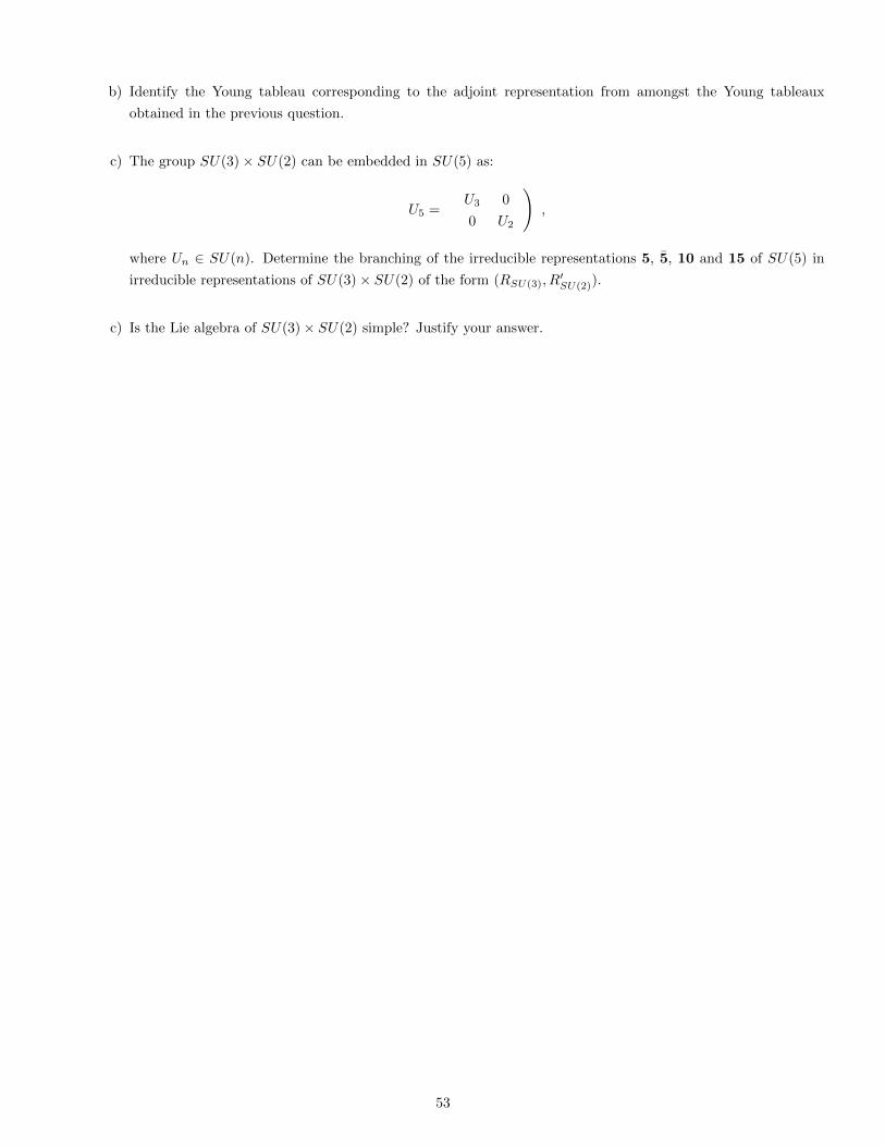
b) Identify the Young tableau corresponding to the adjoint representation from amongst the Young tableaux

obtained in the previous question.

c) The group SU(3)× SU(2) can be embedded in SU(5) as:

U5 =

(U3 0

0 U2

),

where Un ∈ SU(n). Determine the branching of the irreducible representations 5, 5, 10 and 15 of SU(5) in

irreducible representations of SU(3)× SU(2) of the form (RSU(3), R′SU(2)).

c) Is the Lie algebra of SU(3)× SU(2) simple? Justify your answer.

53