Lie and Kac-Moody algebras

Ella Jamsin and Jakob Palmkvist

Physique Theorique et Mathematique,Universite Libre de Bruxelles & International Solvay Institutes,

ULB-Campus Plaine C.P. 231, B-1050, Bruxelles, Belgium

e-mail: ejamsin@ulb.ac.be, jakob.palmkvist@ulb.ac.be

Based on lectures given by the authors at the Fifth International Modave Summer School onMathematical Physics, held in Modave, Belgium, August 2009.

Abstract

In these lectures, we present in a selfcontaining way an introduction to the theory of Lieand Kac-Moody algebras. Throughout the text, we mainly focus on the concepts thatare important in applications to mathematical physics, especially in the context of hiddensymmetries.

Contents

1 Introduction 31.1 Outline . . . . . . . . . . . . . . . . . . . . . . . . . . . . . . . . . . . . . . 31.2 References . . . . . . . . . . . . . . . . . . . . . . . . . . . . . . . . . . . . . 3

2 General definitions 42.1 Lie algebra, structure constants, adjoint representation . . . . . . . . . . . . 42.2 Ideal, abelian/simple/semisimple algebras . . . . . . . . . . . . . . . . . . . 5

3 Simple finite-dimensional Lie algebras 53.1 The Cartan subalgebra . . . . . . . . . . . . . . . . . . . . . . . . . . . . . . 63.2 Weights of a representation and roots . . . . . . . . . . . . . . . . . . . . . 63.3 Cartan-Weyl basis . . . . . . . . . . . . . . . . . . . . . . . . . . . . . . . . 73.4 The Killing form . . . . . . . . . . . . . . . . . . . . . . . . . . . . . . . . . 73.5 Root chains and properties of roots . . . . . . . . . . . . . . . . . . . . . . . 83.6 Euclidean structure on the roots . . . . . . . . . . . . . . . . . . . . . . . . 93.7 Positive roots and the triangular decomposition . . . . . . . . . . . . . . . . 103.8 Restrictions on angles and norms . . . . . . . . . . . . . . . . . . . . . . . . 103.9 Simple roots and their properties . . . . . . . . . . . . . . . . . . . . . . . . 113.10 Cartan matrix and Dynkin diagram . . . . . . . . . . . . . . . . . . . . . . 123.11 Classification . . . . . . . . . . . . . . . . . . . . . . . . . . . . . . . . . . . 133.12 Root diagrams . . . . . . . . . . . . . . . . . . . . . . . . . . . . . . . . . . 173.13 Application: Hidden symmetries . . . . . . . . . . . . . . . . . . . . . . . . 19

4 Generalisation to Kac-Moody algebras 224.1 Generalisation of the Cartan matrix . . . . . . . . . . . . . . . . . . . . . . 224.2 The Chevalley-Serre relations . . . . . . . . . . . . . . . . . . . . . . . . . . 244.3 The Killing form revisited . . . . . . . . . . . . . . . . . . . . . . . . . . . . 254.4 Roots of Kac-Moody algebras . . . . . . . . . . . . . . . . . . . . . . . . . . 254.5 The Chevalley involution . . . . . . . . . . . . . . . . . . . . . . . . . . . . . 254.6 Examples . . . . . . . . . . . . . . . . . . . . . . . . . . . . . . . . . . . . . 26

5 Affine algebras 265.1 Definition and Cartan matrix . . . . . . . . . . . . . . . . . . . . . . . . . . 265.2 Classification of affine Lie algebras . . . . . . . . . . . . . . . . . . . . . . . 275.3 Infinite-dimensional algebras . . . . . . . . . . . . . . . . . . . . . . . . . . 285.4 Coxeter labels and central element . . . . . . . . . . . . . . . . . . . . . . . 295.5 Untwisted affine algebras as the central extension of a loop algebra . . . . . 295.6 Twisted affine algebras . . . . . . . . . . . . . . . . . . . . . . . . . . . . . . 30

6 Representations and the Weyl group 316.1 Representations of sl(2) . . . . . . . . . . . . . . . . . . . . . . . . . . . . . 316.2 Highest weight representations . . . . . . . . . . . . . . . . . . . . . . . . . 326.3 Implications for the root system . . . . . . . . . . . . . . . . . . . . . . . . . 346.4 Integrable representations . . . . . . . . . . . . . . . . . . . . . . . . . . . . 356.5 The Weyl group . . . . . . . . . . . . . . . . . . . . . . . . . . . . . . . . . . 36

2

1 Introduction

This introduction to Lie and Kac-Moody algebras is meant to contain tools that are nec-essary when using this theory in mathematical physics, and in particular in the contextof hidden symmetries. The first example of such a symmetry was emphasized by Ehlersin the context of four-dimensional pure gravity [?]. Assuming the existence of one Killingvector and compactifying the metric on the associated circle, one finds a three-dimensionaltheory that has a global symmetry under the Lie algebra sl(2) which is bigger than theexpected u(1). The appearance of such hidden symmetries could then be generalized toother gravity and supergravity theories in various dimensions. As finite-dimensional simpleLie algebras can be completely classified, one can also completely classify the theories thatpossess a hidden symmetry under these algebras [?]. A famous example is the E8 symmetryof D = 11 supergravity in the presence of eight commuting Killing vectors.

Geroch first noticed [?] the appearance of an infinite-dimensional symmetry when twocommuting Killing vectors are assumed in four-dimensional gravity. This symmetry algebrawas later identified as the affine extension of sl(2), the simplest example of an infinite-dimensional Kac-Moody algebra [?]. More generally, one can see that any theory thatpossesses a hidden symmetry under a finite-dimensional Lie algebra g in three dimensionscan be seen to be symmetric under the affine extension of g in two dimensions [?]. Moreover,the two-dimensional theory is integrable.

When one more commuting Killing vector is assumed, that is, when all fields are as-sumed to depend only on one parameter, these theories then show a yet larger infinite-dimensional symmetry algebra, which is called hyperbolic (See [?] and references therein).

1.1 Outline

The lecture notes are organized as follows. Section 2 very shortly presents general andusually known definitions to get started. We then in section 3 review in some detailsthe important tools that appear in the study of finite-dimensional simple Lie algebras. Inparticular, their full classification is presented as well as their appearance in the context ofhidden symmetries. Section 4 explains how the theory can be generalized to describe alarger class of algebras, called Kac-Moody algebras, which can also be infinite-dimensional.The simplest infinite-dimensional Lie algebras, namely affine Lie algebras, are dicussed indetails in section 5. Finally, in section 6, we discuss some more important aspects: wedescribe some representations of Kac-Moody algebras and define the Weyl group.

1.2 References

The references mainly used for finite-dimensional Lie algebras are the books [?] by J. Fuchsand C. Schweigert and [?] by Bauerle and de Kerf. The former is a very nice introductioninto the subject, especially intended for physicists while the latter is more formal and givesa detailed and very clear presentation of the classification of finite-dimensional simple Liealgebras. We also made used of the book [?] by Humphreys. For Kac-Moody algebras, wemade large use of the book [?] by V. Kac which we recommend for the reader who wantsto look up more details.

3

2 General definitions

To get started, this short section contains very general definitions.

2.1 Lie algebra, structure constants, adjoint representation

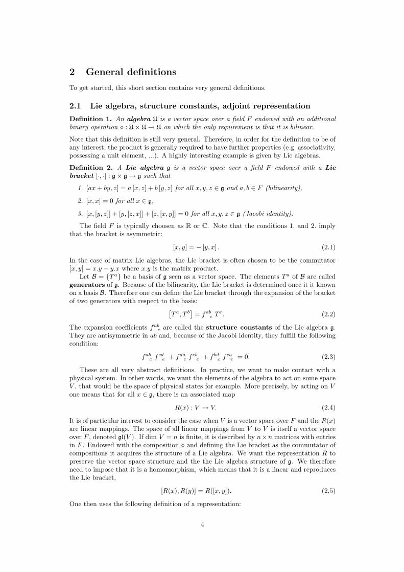
Definition 1. An algebra U is a vector space over a field F endowed with an additionalbinary operation � : U× U→ U on which the only requirement is that it is bilinear.

Note that this definition is still very general. Therefore, in order for the definition to be ofany interest, the product is generally required to have further properties (e.g. associativity,possessing a unit element, ...). A highly interesting example is given by Lie algebras.

Definition 2. A Lie algebra g is a vector space over a field F endowed with a Liebracket [·, ·] : g× g→ g such that

1. [ax+ by, z] = a [x, z] + b [y, z] for all x, y, z ∈ g and a, b ∈ F (bilinearity),

2. [x, x] = 0 for all x ∈ g,

3. [x, [y, z]] + [y, [z, x]] + [z, [x, y]] = 0 for all x, y, z ∈ g (Jacobi identity).

The field F is typically choosen as R or C. Note that the conditions 1. and 2. implythat the bracket is asymmetric:

[x, y] = − [y, x] . (2.1)

In the case of matrix Lie algebras, the Lie bracket is often chosen to be the commutator[x, y] = x.y − y.x where x.y is the matrix product.

Let B = {T a} be a basis of g seen as a vector space. The elements T a of B are calledgenerators of g. Because of the bilinearity, the Lie bracket is determined once it it knownon a basis B. Therefore one can define the Lie bracket through the expansion of the bracketof two generators with respect to the basis:[

T a, T b]

= fabc Tc. (2.2)

The expansion coefficients fabc are called the structure constants of the Lie algebra g.They are antisymmetric in ab and, because of the Jacobi identity, they fulfill the followingcondition:

fabc fcde + fdac f

cbe + f bdc f

cae = 0. (2.3)

These are all very abstract definitions. In practice, we want to make contact with aphysical system. In other words, we want the elements of the algebra to act on some spaceV , that would be the space of physical states for example. More precisely, by acting on Vone means that for all x ∈ g, there is an associated map

R(x) : V → V. (2.4)

It is of particular interest to consider the case when V is a vector space over F and the R(x)are linear mappings. The space of all linear mappings from V to V is itself a vector spaceover F , denoted gl(V ). If dim V = n is finite, it is described by n×n matrices with entriesin F . Endowed with the composition ◦ and defining the Lie bracket as the commutator ofcompositions it acquires the structure of a Lie algebra. We want the representation R topreserve the vector space structure and the the Lie algebra structure of g. We thereforeneed to impose that it is a homomorphism, which means that it is a linear and reproducesthe Lie bracket,

[R(x), R(y)] = R([x, y]). (2.5)

One then uses the following definition of a representation:

4

Definition 3. A representation R of a Lie algebra g on a representation space Vis given by a homomorphism of Lie algebras R : g → gl(V ). If R is injective, then therepresentation is said to be faithful.

Obviously, the trivial representation, that associates the zero map to any element of thealgebra, exists for any Lie algebra. There is also a non-trivial representation that exists forany Lie algebra, the adjoint representation, that acts on the vector space g itself:

Rad : g→ gl(g) : x→ ad x, (2.6)

with the map ad x defined as

(ad x)(y) = [x, y] . (2.7)

Other ways to construct representations will be seen in section 6.

2.2 Ideal, abelian/simple/semisimple algebras

Let us first introduce a notation for subsets h, l of a Lie algebra:

[h, l] ≡ spanF {[x, y] |x ∈ h, y ∈ l} (2.8)

Using this notation one can easily make the following definitions:

Definition 4. A (Lie) subalgebra h of a Lie algebra g is a subset of g that is also a Liealgebra: h ⊆ g and [h, h] ⊆ h.

Definition 5. (i) A subalgebra h of a Lie algebra g is called an ideal iff [h, g] ⊆ h.(ii) A proper ideal is an ideal that is neither equal to {0} nor to g itself

(which are two generic ideals of g).

Definition 6. (i) A Lie algebra g is said to be abelian iff [g, g] = {0}.(ii) A Lie algebra g is said to be simple iff it is not abelian and contains

no proper ideal.(iii) A direct sum of simple Lie algebras is called semisimple. A direct

sum of simple and abelian Lie algebras is called reductive.

Note that any one-dimensional Lie algebra is abelian. Up to an isomorphism, thereexists only one one-dimensional Lie algebra, commonly noted u(1). Moreover, any d-dimensional abelian Lie algebra gAb is isomorphic to the direct sum of d one-dimensionalabelian Lie algebras

gAb =d⊕i=1

u(1). (2.9)

Therefore, the non-trivial part of the classification of reductive algebras is the classificationof simple Lie algebras. It will be the treated in the next section.

3 Simple finite-dimensional Lie algebras

In this section, we restrict to the case of semisimple finite-dimensional Lie algebras. Wewill see how to characterize and classify them.

5

3.1 The Cartan subalgebra

A first fundamental structure of Lie algebras is the Cartan subalgebra, which is a maximalabelian subalgebra. A more precise characterisation requires a few other definitions first.

Definition 7. An element x of a Lie algebra g is called a semisimple element of g ifit has the property that the map adx is diagonizable, that is, if there is a choice of basisB = {T a} such that [x, T a] is proportional to T a for any element of B.

Definition 8. A field F is algebraically closed if any algebraic equation with coefficientsin F has a solution in F .

For example R is not algebraically closed but C is.

Theorem 1. Every semisimple Lie algebra g over an algebraically closed field F containssemisimple elements x.

Proof. When comparing the general relation [x, T a] = MabT

b to the equation for asemisimple element [x, T a] = λT a, one sees that λ must be a solution of the secular orcharacteristic equation det (M − λ1) = 0. This equation is ensured to have a solution if Fis algebraically closed. �

From now on we will assume that F = C, so that we consider complex Lie algebras.The study of real Lie algebras, for which F = R is considerably harder.

One can now define a key concept in the study and classification of semisimple complexLie algebras:

Definition 9. A Cartan subalgebra h of a semisimple Lie algebra g is a maximal abeliansubalgebra consisiting entirely of semisimple elements.

By maximal, we mean that it is not included in a bigger abelian subalgebra with thesame property. This subalgebra is constructed by choosing, among the semisimple elements,a maximal set of linearly independent elements, denoted by Hi, which possess zero Liebrackets among themselves,[

Hi, Hj]

= 0 for i, j = 1, 2, . . . , r. (3.1)

These elements Hi form a basis of a Cartan subalgebra h.A semisimple Lie algebra can possess many different Cartan subalgebras. However, they

are all related by automorphisms of g, so that the freedom in choosing a Cartan subalgebradoes not lead to any arbitrariness in the description of semisimple Lie algebras. Moreover,all Cartan subalgebras have the same dimension r, that is accordingly a property of theLie algebra g and is called its rank.

3.2 Weights of a representation and roots

Let R be a representation of g and h an element of the Cartan subalgebra h of g. Let usassume that Rh ≡ R(h) has an eigenvalue µ(h) for the eigenvector fµ,A, where the indexA stands for a possible degeneracy of the eigenvalue µ(h). Thus one has

Rh(fµ,A) = µ(h)fµ,A. (3.2)

The eigenvalue µ(h) is a complex number that depends linearly on h, and hence µ is alinear function h→ C. By definition, the space of linear maps from a vector space V to thebase field F is called the dual vector space V ? of V . Thus, µ is an element of the vectorspace h? dual to h. It is called a weight of the representation R.

As the generators Hi of a Cartan subalgebra h have zero Lie brackets among eachother,the adjoint maps of all elements of the Cartan subalgebra are simultaneously diagonalizable.

6

As a consequence, there exists a basis of generators of g that are all eigenvectors of themaps ad h for all h ∈ h. In other words, g is spanned by elements y that satisfy

[h, y] = αy(h)y. (3.3)

The functions αy(h) are the weights of the adjoint representation of the Cartan subal-gebra and if they do not vanish they are called the roots of the Lie algebra g. The set ofall roots of a Lie algebra is called the root system and is here denoted ∆. It is includedin h? (and has the same dimension r). Moreover, on can prove that vanishing weightscorrespond to elements of the Cartan subalgebra: [h, x] = 0 for all h ∈ h⇒ x ∈ h. This isequivalent to saying that the centralizer of h in g is h itself. (The proof can for example befound in section 8.2 of [?].)

3.3 Cartan-Weyl basis

Because all generators of g satisfy the relation (3.3) and because all vanishing weightscorrespond to elements of the Cartan subalgebra, the Lie algebra can be written as a directsum of vector spaces according to

g = h⊕⊕α∈∆

gα, gα = {x ∈ g| [h, x] = α(h)x ∀ h ∈ h}. (3.4)

The dimension of gα is called the multiplicity of the root α. In the case of simplefinite-dimensional Lie algebras, one can show that the multiplicity of any root is one. Asa consequence, each root α determines, up to a normalization, one basis element of thealgebra, here denoted Eα, sometimes called a step operator. A full basis of generators ofthe Lie algebra g is accordingly given by

BCW = {Hi | i = 1, . . . , r} ∪ {Eα | α ∈ ∆}, (3.5)

with the commutation relations[Hi, Hj

]= 0,

[Hi, Eα

]= α(Hi)Eα for α ∈ ∆, (3.6)

where α(Hi) is non-vanishing for at least one value of i. A basis of this form is called aCartan-Weyl basis of g. Note that if

[Eα, Eβ

]6= 0, then

[Eα, Eβ

]∝ Eα+β .

3.4 The Killing form

To analyse further the root system ∆, one will need to define an inner product on ∆. Thiscan be done by first defining an analogous structure on its dual space h, that can in turnbe otained as the restriction of a bilinear form on the whole algebra g. It must possess theproperties of symmetry, bilinearity and invariance (or associativity). The latter conditionmeans that, for all x, y, z ∈ g,

κ([x, y] , z) = κ(x, [y, z]). (3.7)

For simple finite-dimensional Lie algebras, one can see that, up to an overall factor,there is a unique invariant symmetric bilinear form, given by

κ(x, y) = tr(ad x ◦ ad y) (3.8)

where ◦ denotes the composition of maps and tr is the trace of linear maps. This bilinearform is called the Killing form.

For an arbitrary finite Lie algebra, the Killing form κ can be degenerate, i.e. theremay exist elements x 6= 0 in g such that κ(x, y) = 0 for all y ∈ g. It that case, κ will notlead to proper inner product in H?. However, Cartan proved the important result that a

7

finite-dimensional Lie algebra g is semisimple if and only if κ is non-degenerate. Moreover,te restriction of κ on the Cartan subalgebra h is also non-degenerate.

Using the Killing form, one can define a vector space isomorphism

ν : h ∈ h→ νh ∈ h? (3.9)

between h and its dual h? in the following way:

νh(h′) := κ(h, h′). (3.10)

The element of h mapped to the root α by the isomorphism ν is called the star vectorassociated to α and is noted tα:

tα := ν−1(α) ∈ h. (3.11)

It satisfies

α(h) = νtα(h) = κ(tα, h). (3.12)

This will allow us to define a Euclidean inner product in section 3.6.

3.5 Root chains and properties of roots

We will see here a series of theorems about roots of semisimple Lie algebras, providing afirst glance at the important restriction imposed for a element of h? to be a root. Thesetheorems will be crucial for the classification.

Theorem 2. 1. The only multiples of α ∈ ∆ that are roots are ±α.

2. Let α ∈ ∆ and Eα an associated step operator. Then there exists an element Fα thatis a step operator associated to −α such that the set {Eα, Fα, Hα}, where Hα :=[Eα, Fα], spans a three-dimensional simple Lie algebra.

3. The vector Hα satisfies

Hα =2tα

κ(tα, tα)(3.13)

For a proof, see for example the section 6.4 of [?]. Concerning parts 2. and 3. of thetheorem, without actually proving them, let us make some comments. One easily sees that{Eα, Fα, Hα} span an algebra. Indeed,

[Hα, Eα] = α(Hα)Eα, (3.14)[Hα, Fα] = −α(Hα)Fα, (3.15)[Eα, Fα] = Hα. (3.16)

Moreover, with the third part of the theorem and using equation (3.12), one sees thatα(Hα) = 2 and thus one recovers the usual commutation relations of sl(2,C), the Liealgebra of complex 2 × 2 matrices, with the matrix commutator as Lie bracket. Thegenerator Eα plays the role of the positive step operator and Fα the negative one.

Theorem 3. Let g be a complex semisimple Lie algebra. Let α and β 6= ±α be roots andlet M be the set of integers {t} such that β + tα is a root, i.e.

M := {t ∈ Z|β + tα ∈ ∆} (3.17)

8

1. Then M is a closed interval [−p, q] of integers

M = [−p, q] ∩ Z (3.18)

with p and q non-negative integers.

The sequence of roots

β − pα, . . . , β + qα (3.19)

is called the α-chain through β.

2. Moreover on has p− q = β(Hα). In particular, β(Hα) is an integer, called a Cartaninteger:

β(Hα) ∈ Z. (3.20)

This theorem will be proven in section 6.1. Note that β(Hα) = p−q ∈ [−p, q]∩Z = M ,which implies that

β − β(Hα)α ∈ ∆. (3.21)

3.6 Euclidean structure on the roots

Using the theorems 1 and 2 in the preceding section, one can define a Euclidean structureon the roots. Let us first define a symmetric bilinear form on h?:

Definition 10. For α and β ∈ h?, one defines

(α|β) := κ(ν−1(α), ν−1(β)) = κ(tα, tβ). (3.22)

Consider now the real vector space E that is the R-span of ∆:

E :={∑α∈∆

rαα|rα ∈ R}

(3.23)

One can prove that the restriction of the bilinear form (·|·) to the subspace E of h? ispositive-definite and thus non-degenerate. It accordingly corresponds to a Euclidean innerproduct on E. One can then define the norm ||α|| of a root α and the angle φαβ betweentwo roots α and β in the usual way:

||α|| =√

(α|α), (3.24)(α|β) = ||α|| ||β|| cosφαβ . (3.25)

Moreover, the Cartan integers can be rewritten using the inner product:

β(Hα) =2(α|β)(α|α)

∈ Z. (3.26)

Note also that, as a consequence of (3.21) and (3.26), if α, β ∈ ∆, then

β − 2(α|β)(α|α)

α ∈ ∆. (3.27)

This new root is the image of β under a reflection in the hyperplane perpendicular to α. Tosee this, note that the new root can be rewritten as β−2||β||cos φαβ1α, where 1α = α/||α||.This corresponds to a symmetry of the root system and is called a Weyl reflection.

9

3.7 Positive roots and the triangular decomposition

The presence of a euclidean structure on the root system enables us to develop a geometricalpicture of the roots. In particular one can define positive and negative roots and introducea relation of order. A common way to do so is the so-called lexicographical ordering.Consider a basis {αi, i = 1, . . . , r} of the root system ∆, such that any root is given by itscomponents ai in this basis:

α =r∑i=1

aiαi.

Definition 11. (i) α is positive if its first non vanishing component is positive and onethen writes α > 0.

(ii) α is negative if its first non vanishing component is negative and onethen writes α < 0.

(iii) α is greater than β (or β is smaller than α) if α− β > 0. One thenwrites α > β.

Note that a root is always either positive or negative. The set of positive (negative)roots is noted ∆+ (∆−). Moreover, as a consequence of the first property given in Theorem2, one has a root in ∆− for each root in ∆+, and hence we can write

{Eα|α ∈ ∆} = {Eα|α ∈ ∆+} ∪ {E−α|α ∈ ∆+} (3.28)

The step operator associated to a positive root is also called a raising operator, whilethe ones associated to negative roots, E−α, also noted Fα, are called lowering operator.Note that the way you divide the roots in positive and negative ones depends on the choiceof a criterium, and in the choice made here, it still depends on the choice of a basis. Inany case, it also follows from the property above that the number of elements in ∆+ (orin ∆−) is equal to d−r

2 if the Lie algebra is of dimension d and rank r. In particular, itimplies that the difference d− r between the dimension and the rank of g is always even.

In addition, it can be seen easily that the subspace of g that is spanned by the stepoperators for positive (negative) roots is in fact a subalgebra. It will be denoted here asn+ (n−) and is called a nilpotent subalgebra of g. According to the decompositions (3.4)and (3.28), g can be written as the following direct sum of vector spaces:

g = n− ⊕ h⊕ n+. (3.29)

This is called the triangular or Cartan decomposition.

3.8 Restrictions on angles and norms

As already stated, once given the inner product (·|·), one can define the norm ||α|| of a rootα and the angle φαβ between two roots α and β in the usual way:

||α|| =√

(α|α), (3.30)(α|β) = ||α|| ||β|| cosφαβ . (3.31)

A first step towards the full classification of finite dimensional semi-simple Lie algebras isto see the norm and angles of roots can only take certain values. To obtain the restrictions,consider two Cartan integers M and N defined from two roots α and β with β 6= ±α as

M :=2(α|β)(α|α)

, N :=2(α|β)(β|β)

. (3.32)

10

Notice that M and N have the same sign, so that their product is a natural number MN∈ N. Moreover

MN = 4 cos2φαβ . (3.33)

As a consequence,

0 ≤MN < 4. (3.34)

The second inequality is strict because the equality woul correspond to β = ±α. Onetherefore has that a Cartan integer can only take the values 0,±1,±2,±3. The angle isalso constrained to the values such that cos2φαβ ∈ {0, 1

4 ,12 ,

34}. The ratio between the

norms of β and α is given by the formula

||β||||α||

=

√M

N. (3.35)

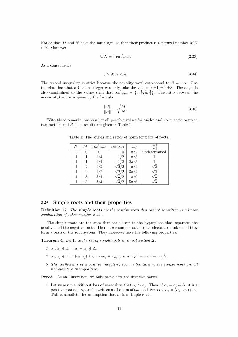
With these remarks, one can list all possible values for angles and norm ratio betweentwo roots α and β. The results are given in Table 1.

Table 1: The angles and ratios of norm for pairs of roots.

N M cos2φαβ cos φαβ φαβ||β||||α||

0 0 0 0 π/2 undetermined1 1 1/4 1/2 π/3 1−1 −1 1/4 −1/2 2π/3 1

1 2 1/2√

2/2 π/4√

2−1 −2 1/2 −

√2/2 3π/4

√2

1 3 3/4√

3/2 π/6√

3−1 −3 3/4 −

√3/2 5π/6

√3

3.9 Simple roots and their properties

Definition 12. The simple roots are the positive roots that cannot be written as a linearcombination of other positive roots.

The simple roots are the ones that are closest to the hyperplane that separates thepositive and the negative roots. There are r simple roots for an algebra of rank r and theyform a basis of the root system. They moreover have the following properties:

Theorem 4. Let Π be the set of simple roots in a root system ∆.

1. αi, αj ∈ Π⇒ αi − αj /∈ ∆,

2. αi, αj ∈ Π⇒ (αi|αj) ≤ 0 ⇒ φij ≡ φαiαj is a right or obtuse angle,

3. The coefficients of a positive (negative) root in the basis of the simple roots are allnon-negative (non-positive).

Proof. As an illustration, we only prove here the first two points.

1. Let us assume, without loss of generality, that αi > αj . Then, if αi − αj ∈ ∆, it is apositive root and αi can be written as the sum of two positive roots αi = (αi−αj)+αj .This contradicts the assumption that αi is a simple root.

11

2. Consider the αj-chain through αi. As αi − αj is not a root, one has p = 0. As aconsequence, q is such that

− q = αi(Hαj ) =2(αi|αj)(αj |αj)

. (3.36)

It follows that (αi|αj) ≤ 0.

�

3.10 Cartan matrix and Dynkin diagram

From the simple roots, one can determine all the roots of the algebra. The whole algebra isencoded in the Cartan matrix A, whose elements are Cartan integers of the simple rootsas follows:

Aij = 2(αi|αj)(αj |αj)

. (3.37)

All the properties of roots and in particular simple roots detailed in the previous chap-ters lead to a series of properties fulfilled by the Cartan matrix, and that will enable us toclassify all finite semisimple Lie algebras in the following part.

Theorem 5. Let A be the Cartan matrix of a finite-dimensional complex semisimple Liealgebra g. Then

1. A is symmetrizable, that is, there exists a diagonal matrix D such that DA is symmet-ric. Choose for example Dii = 1/(αi|αi). The symmetrized matrix is positive-definite,because the bilinear form (·|·) is.

2. Aii = 2,

3. Aij ∈ {0,−1,−2,−3} (i 6= j)

4. Aij = 0⇔ Aji = 0

5. Aij = −2⇒ Aji = −1

6. Aij = −3⇒ Aji = −1

To a Cartan matrix is associated a Dynkin diagram, consisting of vertices representingthe simple roots and (oriented) lines connecting them. The Dynkin diagram of an algebrag of rank r is constructed using the following rules:

1. Draw r vertices, one for each simple root αi,

2. Connect the vertices i and j with a number of lines equal to max{|Aij |, |Aji|}, orequivalently1 to the product AijAji,

3. If |Aij | > |Aji|, draw an arrow going from vertex i to vertex j (that is from thebiggest to the smallest root).

The non-oriented diagram obtained by taking only the two first rules into account is calleda Coxeter diagram.

1Note that the equivalence between the two conventions for the number of lines between two verticesis only true for finite-dimensional Lie algebras. The first one is more practical for the infinite-dimensionalgeneralizations.

12

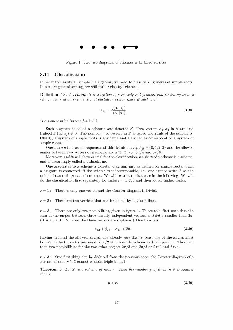
w w w w w wFigure 1: The two diagrams of schemes with three vertices.

3.11 Classification

In order to classify all simple Lie algebras, we need to classify all systems of simple roots.In a more general setting, we will rather classify schemes:

Definition 13. A scheme S is a system of r linearly independent non-vanishing vectors{α1, . . . , αr} in an r-dimensional euclidean vector space E such that

Aij = 2(αi|αj)(αj |αj)

(3.38)

is a non-positive integer for i 6= j.

Such a system is called a scheme and denoted S. Two vectors α1, α2 in S are saidlinked if (αi|αj) 6= 0. The number r of vectors in S is called the rank of the scheme S.Clearly, a system of simple roots is a scheme and all schemes correspond to a system ofsimple roots.

One can see that as consequences of this definition, AijAji ∈ {0, 1, 2, 3} and the allowedangles between two vectors of a scheme are π/2, 2π/3, 3π/4 and 5π/6.

Moreover, and it will show crucial for the classification, a subset of a scheme is a scheme,and is accordingly called a subscheme.

One associates to a scheme a Coxeter diagram, just as defined for simple roots. Sucha diagram is connected iff the scheme is indecomposable, i.e. one cannot write S as theunion of two orthogonal subschemes. We will restrict to that case in the following. We willdo the classification first separately for ranks r = 1, 2, 3 and then for all higher ranks.

r = 1 : There is only one vertex and the Coxeter diagram is trivial.

r = 2 : There are two vertices that can be linked by 1, 2 or 3 lines.

r = 3 : There are only two possibilities, given in figure 1. To see this, first note that thesum of the angles between three linearly independent vectors is strictly smaller than 2π.(It is equal to 2π when the three vectors are coplanar.) One thus has

φ12 + φ23 + φ31 < 2π. (3.39)

Having in mind the allowed angles, one already sees that at least one of the angles mustbe π/2. In fact, exactly one must be π/2 otherwise the scheme is decomposable. There arethen two possiblilities for the two other angles: 2π/3 and 2π/3 or 2π/3 and 3π/4.

r > 3 : One first thing can be deduced from the previous case: the Coxeter diagram of ascheme of rank r ≥ 3 cannot contain triple bounds.

Theorem 6. Let S be a scheme of rank r. Then the number p of links in S is smallerthan r:

p < r. (3.40)

13

Proof. Let S = {α1, . . . , αr} and define χ as

χ =r∑i=1

αi√(αi|αi)

(3.41)

As the ai’s are linearly independent, χ 6= 0. Therefore

0 < (χ|χ) = r + 2∑i<j

cos φij , (3.42)

which means that

r > −2∑i<j

cos φij . (3.43)

The number p of links is equal to the number of times that cos φij 6= 0. But cos φij 6= 0implies −2cos φij ≥ 1 (cf. allowed angles). The right hand side of (3.43) is therefore biggerthan p, and the theorem is proven. �

A consequence of this theorem is the following:

Theorem 7. Schemes do not contain closed circuits (=loops). In other words, they aretree diagrams.

Theorem 8. The number of lines emanating from a vertex of a scheme is at most equalto three.

Proof. Let αi be an element of S and {β1, . . . , βm} the other elements of S that arelinked to αi, that is, such that (αi|βj) 6= 0. The number N of lines emanating from αi isgiven by

N =m∑j=1

nij (3.44)

where

nij = 4(αi|βj)(βj |αi)(βj |βj)(αi|αi)

= 4(αi|γj)2

(αi|αi), (3.45)

where γj = βj/‖βj‖. The γj must be all orthogonal to each other. Indeed, if there exists(γj |γk) 6= 0 for some j 6= k, it means that βj and βk are linked and as a consequence{αi, βj , βk} form a loop. Let us introduce an extra unit vector γ0 that is orthogonal to allγj (or equivalently to all βj) but not to αi. (Such a vector exists because αi, β1, . . . , βmare linearly independent.) One has

(αi|γ0) 6= 0. (3.46)

The set {γ0, γ1, . . . , γm} is an orthonormal set. Hence

αi =m∑j=0

(αi|γj)γj , (3.47)

and then

(αi|αi) =m∑j=0

(αi|γj)2. (3.48)

14

Going back to N , one finally gets

N = 4m∑j=0

(αi|γj)2

(αi|αi)− 4

(αi|γ0)2

(αi|αi)= 4− 4

(αi|γ0)2

(αi|αi)< 4. (3.49)

�

As a consequence of this theorem, a vertex of the Coxeter diagram of a scheme can haveeither up to three single links or one double link and possibly another single link. The caseof a vertex with three single links is called a node.

Definition 14. One calls a chain a (sub)scheme {δ1, . . . , δm|m > 2} such that all thepairs {δi, δi+1} are linked. The chain is homogeneous if the links are all single.

Theorem 9. Let S be a scheme containing a chain {δ1, . . . , δm}. Then the system obtainedby replacing the chain {δ1, . . . , δm} by a single vector δ =

∑mi=1 δi is also a scheme. From

the point of view of the Coxeter diagram, the new scheme is obtained by shrinking the chainto one vertex.

Proof. We have to prove two things : first that the vectors of the new scheme are linearlyindependent and second that the matrix elements Aij are non-positive integers for i 6= j inthe new scheme.

Let us note S′ = S\{δ1, . . . , δm}. If S = S′ ∪ {δ1, . . . , δm} is linearly independent, it isclear that S′ ∪ {δ} is linearly independent too.

For the second part, we only need to check the matrix elements relating vectors of S′

to δ. We therefore consider 2 (δ|αi)(αi|αi) and 2 (δ|αi)

(δ|δ) where αi ∈ S′. First note that αi can onlybe linked to one of the vertices of the chain, otherwise there exists a loop in the diagram.Consequently, (δ|αi) = (δk|αi) for some k.

The first element we consider is

2(δ|αi)(αi|αi)

= 2(δk|αi)(αi|αi)

. (3.50)

It is non-positive because S is a scheme.For the second matrix element, we need to compute (δ|δ).

(δ|δ) = (δm|δm) +m−1∑j=1

{(δj |δj) + 2(δj |δj+1)} (3.51)

= (δm|δm) +m−1∑j=1

{(δj |δj)− (δj |δj)} (3.52)

= (δk|δk). (3.53)

From (3.51) to (3.52), one uses that

2(δj |δj+1)(δj |δj)

= −1.

From (3.52) to (3.53), one uses that in a chain, all vertices have the same norm. Usingwhat precedes, one then finds that the second matrix element to check is

2(δ|αi)(δ|δ)

= 2(δk|αi)(δi|δi)

, (3.54)

which is non positive because S is a scheme. �

Theorems 8 and 9 directly imply the following restriction:

15

w w ww w ww w!!!aaa

www w w

w w!!!aaa

www waa

a!!!

ww

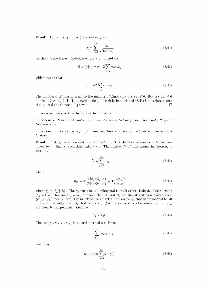
Figure 2: These three diagrams cannot be subdiagrams of schemes because, up to theshrinking of a chain to a vertex, they are equivalent to diagrams with four vertices ema-nating from a vertex.

w w w w w ww w w w w w

I

II

III w w w!!!aaa

ww

w ww w

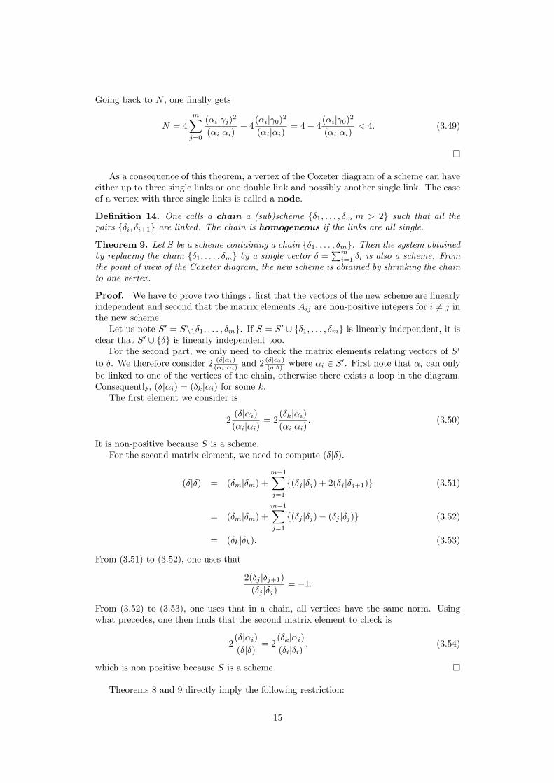
Figure 3: These classes of diagrams of indecomposable schemes.

Theorem 10. The Coxeter diagram of a scheme does not contain a subdiagram of the typedepicted in figure 2.

Let us summarize the current state of the classification. Any Coxeter diagram of anindecomposable scheme S is a tree diagram with one the following alternatives:

1. It has no double link and no node. Then it has only single links (see class I in figure3),

2. It has one double link, then it has no node (see class II in figure 3).

3. It has one node, then it has no double link (see class III in figure 3).

To all diagram of class I with k vertices corresponds a scheme, whose A matrix is givenby Aii = 2 and Aij = −1 for i 6= j. The corresponding Lie algebra is denoted Ak. (cf.figure 6)

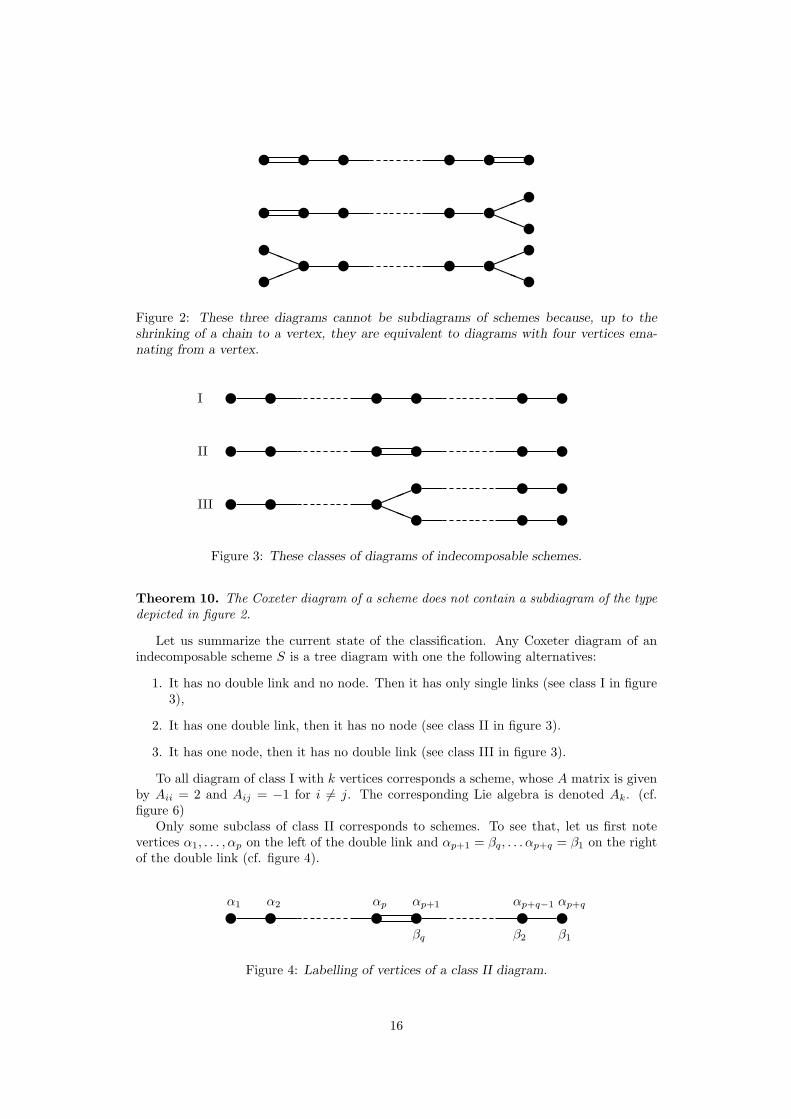
Only some subclass of class II corresponds to schemes. To see that, let us first notevertices α1, . . . , αp on the left of the double link and αp+1 = βq, . . . αp+q = β1 on the rightof the double link (cf. figure 4).

w w w w w wα1 α2 αp αp+1 αp+q−1 αp+q

βq β2 β1

Figure 4: Labelling of vertices of a class II diagram.

16

α1 α2 αp δβq β2 β1

γr γ2 γ1w w w w!!!aaa

ww

w ww w

Figure 5: Labelling of vertices of a class III diagram.

One has Ap,p+1Ap+1,p = 2. Let us assume, without loss of generality that Ap,p+1 = −1and Ap+1,p = −2, implying that

(αp+1|αp+1) = (βq|βq) = 2(αp|αp),

and let us set(αi|αi) = a, i = 1, . . . , p.

Let us moreover define

α =p∑i

iαi β =q∑j

jβj .

Since α an β are linearly independent, we have

(α|β)2 < (α|α)(β|β).

By calculating each factor in this inequality, one can show that it is equivalent to

(p− 1)(q − 1) < 2.

As a consequence there are only three admissible subclasses (cf figure 6)

• p = 1 and q = 1, 2, . . . , the corresponding Lie algebras being Bq+1,

• q = 1 and p = 1, 3, . . . , the corresponding Lie algebras being Cq+1,

• q = 2 and p = 2, the corresponding Lie algebra beging F4.

In class III, calling δ the vertex at the center of the node and α1, . . . αp, β1, . . . , βq andγ1, . . . , γr the three chains of vertices around it (cf figure 5), defining then α and β as beforeand γ in a similar fashion, the important inequality in this case will be that

cos2αδ + cos2βδ + cos2γδ < 1,

where αδ is the angle between α and δ. This inegality can be deduced from the fact thatα, β and γ are orthogonal and δ does not belong to their linear span.

At the end of the day, one finds that only the following possibilities exist (cf figure 6)

• r = 1, q = 1 and p = 1, 2, . . . , that correspond to the algebras Dp+3,

• r = 1, q = 2 and p = 2, 3, 4, that correspond to the algebras Ep+4.

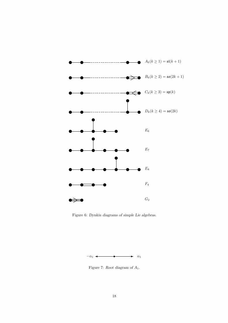
3.12 Root diagrams

For algebras with rank r = 1 or 2, the roots can be represented by a diagram on a plane.For r = 1, there is only one simple root, α, and the only other possible root is −α. Itcorresponds to A1 and the root diagram is presented in figure 7.

For r = 2, there are two simple roots, α1 and α2. The angle between them can onlytake four values:

17

w w w w Ak(k ≥ 1) = sl(k + 1)

w w w w Bk(k ≥ 2) = so(2k + 1)b"

w w w w Ck(k ≥ 3) = sp(k)"b

w w w ww

Dk(k ≥ 4) = so(2k)

w w w w ww

E6

w w w w w ww

E7

w w w w w w ww

E8

w w w w F4

w wb"

G2

Figure 6: Dynkin diagrams of simple Lie algebras.

s -� α1−α1

Figure 7: Root diagram of A1.

18

s s-�

6

?

α1−α1

α2

−α2

Figure 8: Root diagram of A1 ⊕A1.

s -��

JJJJ]

�

JJJJ

α1

α2 α1 + α2

Figure 9: Root diagram of A2.

1. φα1α2 = π/2 ⇒ ratio of norms undetermined,

2. φα1α2 = 2π/3 ⇒ roots of equal lengths,

3. φα1α2 = 3π/4 ⇒ two different lengths,

4. φα1α2 = 5π/6 ⇒ two different lengths.

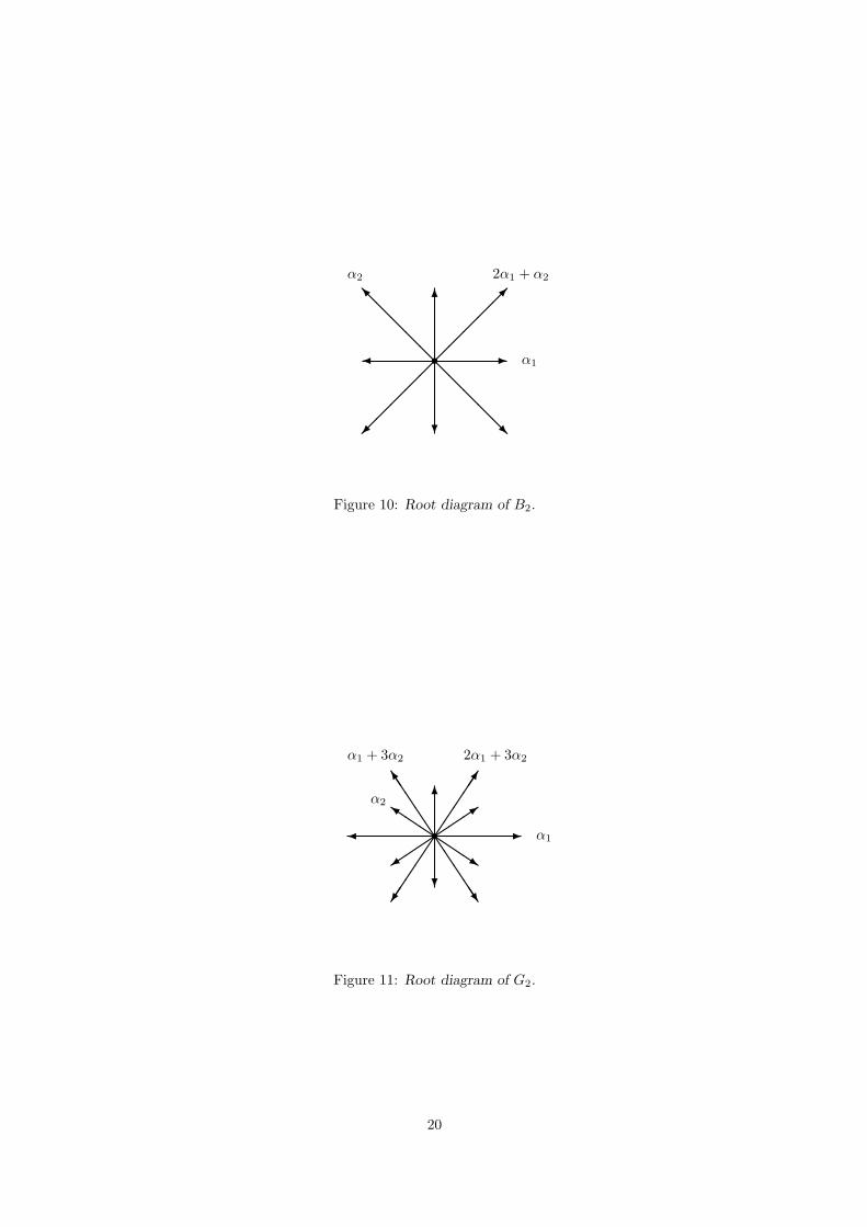
By use of Weyl reflections, all other roots can then be found. The cooresponding algebrasare respectively A1 ⊕A1, A2, B2 and G2. The roots diagram are in figure 8 to 11.

3.13 Application: Hidden symmetries

In the presence of n commuting Killing vectors, or in other words, when compactified on an-torus, a D-dimensional theory can be seen as a D − n theory that will contain a certainnumber of scalar fields. It is a remarkable fact that in several cases, these scalar fields forma non-linear sigma model that is symmetric under a simple finite-dimensional algebra. Inparticular, if n = D − 3, the reduced theory is in three dimensions and all p-form fieldscan be dualised to scalars. The three-dimensional theory is then only three-dimensionalgravity plus scalars forming a non-linear sigma model with the target space being G/Kwhere G is the group obtained by exponentiation of a simple finite-dimensional Lie algebrag and K its maximal compact subgroup. In this section, we only consider the case whenthe reduction is performed on spatial coordinates. The definition of K is slightly morecomplicated in other cases.

19

s -��

��

��

@@@

@@I

������

@@@@@R

6

?

α1

α2 2α1 + α2

Figure 10: Root diagram of B2.

s -��

JJJJJ]

�

JJJJJ

6

?

���+

QQQk

���3

QQQs

α1

α2

α1 + 3α2 2α1 + 3α2

Figure 11: Root diagram of G2.

20

Let us first review the construction [?] of a non-linear sigma model on the target spaceG/K. We will consider physical examples afterwards. Remember that a d-dimensionalrank r Lie algebra g can be decomposed as

g = n− ⊕ h⊕ n+. (3.55)

where n− is generated by the F i generators, n+ by the Ei and h is spanned by the CartangeneratorsHa (i = 1, . . . , d−r2 ; a = 1, . . . , r). Let us now define the generatorsKi = Ei−F i,that generate the algebra k. The Lie algebra g can now also be decomposed as

g = k⊕ h⊕ n+. (3.56)

This is called the Iwasawa decomposition. It has a corresponding decomposition at thelevel of the group

G = K ×H ×N+. (3.57)

This means that any element in the group G can be written as the product of elements inK, H and N+.

Now, the coset space G/K, that if we want to be accurate should rather be writtenK\G, is the space of left equivalence classes of G under K. That is, one identifies twoelements of G if they differ by an element of K:

g, g′ ∈ G : g ∼ g′ ⇔ g′ = gk g for gk ∈ K. (3.58)

Each class will be represented by an element, that one can choose as

V = g0 g+ (3.59)

where g0 ∈ H and g+ ∈ K. In terms of algebra elements one therefore has

V = ePa Aa(x)Hae

Pi Bi(x)Ei . (3.60)

where Aa(x) and Ba(x) are some functions of the base space coordinates x. To constructthe corresponding Lagrangian, consider first the algebra element V−1dV and decompose itinto a part in k and the rest:

V−1dV = Q+ P (3.61)

where Q ∈ k and P ∈ g k is the component of V−1dV that is parallel to the coset space.One can now write a Lagrangian that is manifestly invariant under global G transformationand local K transformation as

Lcoset = −12

Tr(?P ∧ P) . (3.62)

Let us now consider some example from physics and see how they fit in this picture.

Pure 5D gravity The field content in five dimensions is of course just a metric g(5)µν .

After reduction to three dimensions, one is left with a three dimensional metric gmn,two one-forms V (1)

m and V(2)m and three scalars: two dilatons φ1, φ2 and one axion χ1.

Schematically2, they are obtained from the five-dimensional metric as follows

g(5)µν =

gmn V

(1)m V

(2)m

V(1)n φ2 χ1

V(2)n χ1 φ1

(3.63)

2In practice, a less naive reduction ansatz is needed in order make the underlying symmetry transparent.The lectures on Kaluza-Klein theory by Pope [?] give a clear introduction to dimensional reductions.

21

The two one-forms can be dualised into scalars χ2 and χ3 through an expression of theform

dmVn = εmnpdpχ. (3.64)

As a consequence one is left with a metric, two dilatons and three axions. The identificationwith a non linear sigma model is done by associating the dilatons to Cartan generators andthe axions to positive step operators, or positive roots. As a consequence, in this case, oneneed an algebra that has rank two and dimension d = 2 + 2.3 = 8. Such an algebra is givenby A2 = sl(3). Its compact subalgebra is so(3).

Now, more precisely, in order to prove that the scalars form a non linear sigma model,one must choose as a coset representative

V = ePa φa(x)Hae

Pi χi(x)Ei , (3.65)

then compute the corresponding Lagrangian and compare it to the physical Lagrangianobtained after dimensional reduction and dualisation of the vectors. This process requiresa series of extra subtleties that are outside the scope of these lectures.

5D minimal supergravity 5D minimal supergravity describes 5D gravity in presenceof matter fields. Besides a five dimensional metric, it contains a one-form A

(5)µ , that de-

composes under reduction to 3D into a one-form Am and two axions χ4, χ5:

A(5)µ =

(Am χ4 χ5

)(3.66)

Again, in three dimensions, the one-form Am is dual to a scalar χ6. With the fieldsobtained from the metric, one is accordingly left with a scalar content made of two dilatonsand six axions. An algebra of rank 2 and dimensions 14 exists, that is G2 that has so(4)as a compact subalgebra [?]. One can show that the corresponding sigma model indeedreproduces the scalar part of the Lagrangian of 5D minimal supergravity after reductionto 3D.

4 Generalisation to Kac-Moody algebras

4.1 Generalisation of the Cartan matrix

As we have seen, the classification of simple finite-dimensional Lie algebras is based on theassignment of a square integer Cartan matrix to any such Lie algebra, which is unique upto permutations of the index set labeling rows and columns.

We recall that the requirement that the Lie algebra be simple and finite-dimensionalimplies the following conditions on the corresponding Cartan matrix A:

• The diagonal entries are all equal to 2.

• The off-diagonal entries are all non-positive, with Aij = 0 if and only if Aji = 0.

• The Cartan matrix is indecomposable.

• The Cartan matrix is symmetrizable, and the symmetrized matrix is positive-definite.

By relaxing the last condition one obtains a much larger class of Lie algebras, called Kac-Moody algebras. We will henceforth talk about Cartan matrices in this generalized mean-ing. By definition, each of them gives rise to a Kac-Moody algebra in a unique way that wewill describe. If two Cartan matrices give rise to two isomorphic Kac-Moody algebras, thenthey differ only by a permutation of the index set labeling rows and columns. We will nowreview the classification of Cartan matrices, following [?]. Since there is a one-to-one cor-respondence between Cartan matrices and Kac-Moody algebras this will then correspond

22

to a classification of Kac-Moody algebras. We will then explain how a Kac-Moody algebrais constructed from its Cartan matrix A if detA 6= 0.

For any column matrix a, we write a > 0 if all entries are positive, and a < 0 if allentries are negative. We now define an r × r Cartan matrix A to be

• finite if Ab > 0,

• affine if Ab = 0,

• indefinite if Ab < 0

for some r× 1 matrix b > 0. One and only one of these three assertions is valid for any A,and in the affine case, b is uniquely defined up to normalization. Affine Cartan matricescan also be characterized in the following way.

• A is affine if and only if detA = 0 and deletion of any row and the correspondingcolumn gives a direct sum of finite Cartan matrices.

As we will describe in section 4.2, any Cartan matrix defines uniquely a Lie algebra, andall Lie algebras that can be obtained in this way are called Kac-Moody algebras. Thus wecan say that a Kac-Moody algebra is finite, affine or indefinite if the same holds for itsCartan matrix. Finite Kac-Moody algebras are then nothing but simple finite-dimensionalLie algebras, and their construction gives us back the classification in section 3.11. Also theaffine Kac-Moody algebras are well understood, as certain extensions of finite algebras (seesection 5). On the other hand, the indefinite Kac-Moody algebras are not fully classifiednor well understood. We need to impose further conditions in order to study them alongwith the finite and affine algebras. In what follows we will always require an indefiniteCartan matrix A to be symmetrizable, a requirement that is already satisfied by finite andaffine Cartan matrices. One can then show that

• A is finite if and only if A is symmetrizable and the symmetrized matrix has signature(+ · · ·+ +),

• A is affine if and only if A is symmetrizable and the symmetrized matrix has signature(+ · · ·+ 0 ).

Analogously, we define A to be Lorentzian if A is symmetrizable and the symmetrizedmatrix has signature (+ · · ·+−). (With signature we mean the number of positive, negativeor zero eigenvalues. Their order does not matter.) Clearly, the Lorentzian algebras form asubclass of the class of indefinite algebras, but we can restrict it even further. Similarly tothe characterization of the affine case above, we define hyperbolic Cartan matrices in thefollowing way.

• A is hyperbolic if and only if detA < 0 and deletion of any row and the correspondingcolumn gives a direct sum of affine or finite matrices.

It can be shown that any hyperbolic Cartan matrix is Lorentzian. We say that a Kac-Moody algebra is Lorentzian or hyperbolic if the same holds for its Cartan matrix.

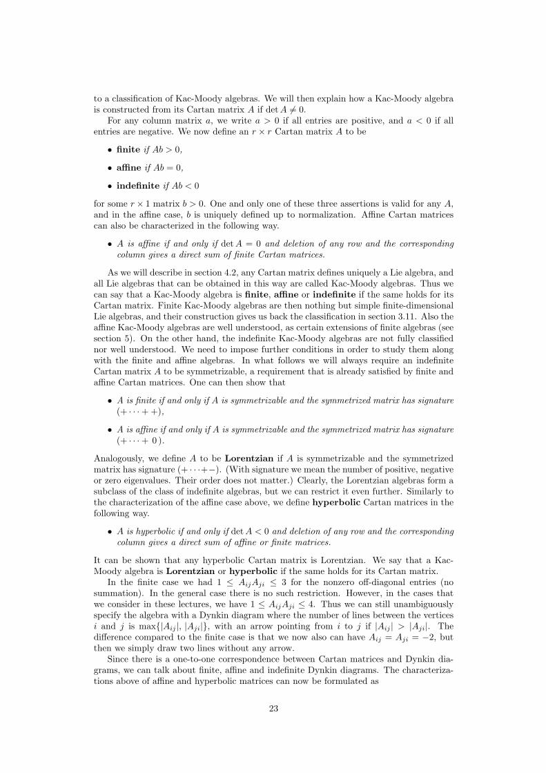
In the finite case we had 1 ≤ AijAji ≤ 3 for the nonzero off-diagonal entries (nosummation). In the general case there is no such restriction. However, in the cases thatwe consider in these lectures, we have 1 ≤ AijAji ≤ 4. Thus we can still unambiguouslyspecify the algebra with a Dynkin diagram where the number of lines between the verticesi and j is max{|Aij |, |Aji|}, with an arrow pointing from i to j if |Aij | > |Aji|. Thedifference compared to the finite case is that we now also can have Aij = Aji = −2, butthen we simply draw two lines without any arrow.

Since there is a one-to-one correspondence between Cartan matrices and Dynkin dia-grams, we can talk about finite, affine and indefinite Dynkin diagrams. The characteriza-tions above of affine and hyperbolic matrices can now be formulated as

23

• A is affine if detA = 0 and deletion of any vertex leads to finite diagrams.

• A is hyperbolic if detA < 0 and deletion of any vertex leads to affine or finite dia-grams.

Permutation of rows and (the corresponding) columns in A corresponds to relabelingthe vertices in the Dynkin diagram. An indecomposable Cartan matrix corresponds to aconnected Dynkin diagram.

4.2 The Chevalley-Serre relations

We will now describe how a Lie algebra can be constructed from a given Cartan matrix Aor, equivalently, from its Dynkin diagram. The Lie algebra g′ obtained in this way is calledthe derived Kac-Moody algebra of A. The Kac-Moody algebra g of A is then definedas a certain extension of g′ in the case when A is affine. We will explain this in section 5.If A is finite or indefinite, then g coincides with g′.

In the construction of the Lie algebra g′ from its Cartan matrix A, one starts with thefact that a simple finite-dimensional Lie algebra is generated by the raising and loweringoperators corresponding to the simple roots αi. These are called Chevalley generatorsand we will henceforth write

ei ≡ Eαi , fi ≡ Fαi . (4.1)

The corresponding Cartan element Hαi = [Eαi , Fαi ] will be called Cartan generatorand denoted

hi ≡ Hαi . (4.2)

(The Cartan generators should not be confused with the tentative basis elements Hi ofthe Cartan subalgebra.) It follows from the definition of the Cartan-Weyl basis (applied tothe simple roots) and the definition of the Cartan matrix, that the Chevalley and Cartangenerators satisfy the Chevalley relations (no summation)

[ei, fj ] = δijhj , [hi, ej ] = αj(hi)ej = 2(αj , αi)(αi, αi)

ej = Ajiej ,

[hi, hj ] = 0, [hi, fj ] = −αj(hi)ej = −2(αj , αi)(αi, αi)

ej = −Ajiej (4.3)

If A is of order r, the derived Kac-Moody algebra g is now defined as the Lie algebragenerated by 3r elements ei, fi, hi modulo the Chevalley relations and the additional Serrerelations (no summation)

(ad ei)1−Ajiej = 0, (ad fi)1−Ajifj = 0. (4.4)

It follows from the Chevalley relations (4.3) that g is spanned by the Cartan generatorsand the set of multiple commutators

[· · · [[ei1 , ei2 ], ei3 ], . . . , eik ], [· · · [[fi1 , fi2 ], fi3 ], . . . , fik ], (4.5)

for all k ≥ 1, which is restricted by the Serre relations (4.4).The number r is called the rank of the (derived) Kac-Moody algebra. In the finite and

indefinite case it coincides with the rank of the Cartan matrix, but if A is an affine Cartanmatrix then it has matrix rank r − 1.

24

4.3 The Killing form revisited

In section 3.4 we defined the symmetric and invariant Killing form of a finite-dimensionalLie algebra as κ(x, y) = tr (ad x ◦ ad y). But if g is simple and finite-dimesional then κcan equivalently, up to an overall factor, be defined by

κ(ei, fj) = Dij , κ(hi, hj) = (DA)ij , (4.6)

for all i, j = 1, 2, . . . , r, where D is a diagonal matrix (unique up to an overall factor)such that DA is symmetric. In all other cases the Killing form is defined to be zero.It can then be extended to the full Cartan-Weyl basis by the symmetry and invarianceproperties, together with the Chevalley relations. (Actually, already the first equationabove is enough.) The Killing form will then be symmetric and invariant by construction,but also non-degenerate. Moreover, these properties define the Killing form uniquely up toautomorphisms and an overall normalization. In section 5 we will see how the Killing formis defined for affine Kac-Moody algebras.

4.4 Roots of Kac-Moody algebras

One can define roots in the same way as for finite Kac-Moody algebras. But there are twoimportant differences:

• The root space, dual to the Cartan subalgebra with respect to the Killing form, isin general not Euclidean. In particular, there can be roots with zero (lightlike) ornegative (timelike) norm.

• The eigenspaces corresponding to the roots (unfortunately also called root spaces) arein general not one-dimensional, so there can be many linear independent root vectorscorresponding to one root. Then the root is said to have multiplicity greater thanone.

The first fact is a simple consequence of allowing for Cartan matrices that are not positive-definite – it follows from the definition of the bilinear form that the signature of the rootspace or the Cartan subalgebra is the same as of the Cartan matrix. The second fact is muchless obvious, but it follows from the Serre relations. It is also a non-trivial consequence ofthe Serre relations that an affine or indefinite Kac-Moody algebra is infinite-dimensional.

4.5 The Chevalley involution

An involution of an algebra is an automorphism that squares to the identity map. DifferentKac-Moody algebras admit different involutions, but it follows from the Chevalley relationsthat there is always an involution given by

ω(hi) = −hi, ω(ei) = −fi, ω(fi) = −ei (4.7)

for the Chevalley generators. It can then be extended to the whole algebra by the homo-morphism property. This involution ω is called the Chevalley involution.

For any automorphism ω of an algebra, the set of elements that are invariant underω constitutes a subalgebra. In the case where ω is the Chevalley involution of a Kac-Moody algebra g, the subalgebra k is called the maximal compact subalgebra. All theelements in this subalgebra have the form x+ ω(x) for all x ∈ g. As we have already seenin section 3.13, this subalgebra (and the corresponding maximal compact subgroup) isvery important in applications where Kac-Moody algebras appear as hidden symmetries.It follows from the definition of the Killing form in the previous subsection that k is alwaysnegative-definite or positive-definite, since the entries in the diagonal matrix D all havethe same sign. Usually they are taken to be positive, so that the Killing form is negative-definite on k. Its orthogonal complement p is the direct sum of the Cartan subalgebra anda positive-definite subspace. The elements in p have the form x− ω(x) for all x ∈ g.

25

4.6 Examples

We end this section with two examples of a Kac-Moody algebra. The simplest example isA1, for which the Dynkin diagram consists of only one vertex, and the Cartan matrix ofonly one entry. We have in this chapter seen how any Kac-Moody algebra is built up fromcopies of A1, corresponding to the different nodes in the Dynkin diagram. The lines andarrows between the nodes tell us how these A1 subalgebras ‘interact’ with each other tobuild up the full Kac-Moody algebra.

For A1 there is only one single root, and this is not enough to build any more positiveroots. Thus A1 is three-dimensional with the Chevalley and Cartan generators correspond-ing to the only simple root as basis elements. The full set of commutation relations for A1

is given by the Chevalley relations corresponding to the only single root:

[h, e] = 2e, [h, f ] = −2f, [e, f ] = h (4.8)

(We have dropped the subscript i = 1, 2, . . . , r since r = 1 in this case.)We turn to our second example of a Kac-Moody algebra, A2, for which the Dynkin

diagram consists of two vertices connected with a single line. Thus the two off-diagonalentries in the Cartan matrix are both equal to −1. Each of the nodes corresponds to anA1 subalgebra, but apart from these two A1 subalgebras there are also the basis elements[e1, e2] and [f1, f2]. On the other hand,

[e1, [e1, e2]] = [e2, [e2, e1]] = [f1, [f1, f2]] = [f2, [f2, f1]] = 0 (4.9)

by the Serre relations, so we cannot construct any more basis elements. Thus A2 is 8-dimensional. The elements eθ = [e1, e2] and fθ = −[f1, f2] form a third A1 subalgebratogether with the Cartan element hθ = h1 + h2 since

[hθ, eθ] = 2eθ, [hθ, fθ] = −2fθ, [eθ, fθ] = hθ. (4.10)

This A1 subalgebra corresponds to the third positive root θ, which is the sum of the twosimple roots: θ = α1 + α2.

5 Affine algebras

5.1 Definition and Cartan matrix

As already explained in section 4.1, an important and quite well known class of Kac-Moodyalgebras is given by affine Lie algebras, defined as follows:

Definition 15. An affine Lie algebra is a Lie algebra constructed out of a so-called affineCartan matrix A, that fulfills the following conditions

• Aii = 2,

• The off diagonal elements are non positive integers and Aij = 0 iff Aji = 0,

• A is symmetrizable,

• detA = 0 and the deletion of any row and the corresponding column gives a directsum of finite Cartan matrices.

The matrix A is thus positive semidefinite with only one vanishing eigenvalue. Thiscondition can be replaced by asking that there exists an invertible diagonal matrix D suchthat DA is symmetric and positive semidefinite. (The requirement already implies thatDA can have at most one zero eigenvalue.)

In the context of Kac-Moody algebras, the rank of an algebra is more generally defined asthe dimension of the Cartan matrix, that, in the case of affine algebras, does not correspond

26

to the dimension of the Cartan subalgebra, as we will see in the following. Note also thatit obviously does not correspond to the rank of the Cartan matrix either.

This way of relaxing the definite positiveness condition on the Cartan matrix happensto be nearly as restrictive as the original requiremement, as we will see immediately thatthe affine algebras can be completely classified and listed on one page.

5.2 Classification of affine Lie algebras

An affine r × r Cartan matrix has rank R = r − 1. Once the classification of finite Cartanmatrices (associated to simple Lie algebras) is known up to some rank, the classification ofaffine Cartan matrices of same rank is straightforward.

For R = 1 (so that r = 2) the problem is very simple: determine the possible nondiagonal entries (non negative and with symmetric zero’s) solving

detA ≡ A11A22 −A21A12 = 4−A21A12 = 0.

One finds two rank r = 2 affine algebras whose Cartan matrices are given by

A(A(1)1 ) =

(2 −2−2 2

)and A(A(2)

1 ) =(

2 −4−1 2

). (5.1)

The notation for the affine algebras is of the form X(n) where X stands for the finiteLie algebra obtained if one removes one row and the corresponding column (any choicein this case, but we have to be more specific at higher ranks). The superscript index (n)characterizes the two different cases: the A(1)

1 is an untwisted affine algebra and A(2)1 is a

twisted one. These two notions will be defined in sections 5.5 and 5.6, where the notation(associated finite algebra and superscript) will then make complete sense.

For R > 1, it is interesting to first notice the following: when one removes a row and thecorresponding column from an affine Cartan matrix, one obtains a finite Cartan matrix.Again if one removes a row and the corresponding column from a finite Cartan matrix, oneobtains a finite Cartan matrix again. As a consequence, the 2 × 2 matrix obtained afterremoving R−2 rows and the corresponding columns from an affine Cartan matrix must beone of the rank two finite Cartan matrices, that correspond to the algebras A1⊕A1, A2, B2

and G2. Therefore, the elements Aij with i 6= j of an affine Cartan matrix can only take thevalues 0,−1,−2,−3 with the extra conditions that AijAji ≤ 3 and Aij = 0 ⇐⇒ Aji = 0.Using these and the vanishing of the global determinant, finding all affine algebras is onlya question of combinatorics.

Example Let us consider as an example the case of an affine algebra of rank 3 andcontaining as a 2×2 submatrix the Cartan matrix of G2. Up to a renumbering of the rowsand columns the affine matrix reads 2 a b

c 2 −3d −1 2

(5.2)

where we have to determine the numbers a, b, c, d fulfilling the above conditions. Thecondition on the determinant reads

detA = 2− a(2c+ 3d) + b(−c− 2d) = 0.

Let us then consider the possible values case by case:

1. a = 0 ⇒ c = 0 ⇒ detA = 2− 2bd ⇒ b = −1 and d = −1.

2. a = −1

27

w w wb"

G(1)2

w w wb"

G(3)2

Figure 12: Dynkin diagrams of G(1)2 and G

(3)2 .

• c = −1 ⇒ detA = 3d+ b+ 2bd ⇒ b = d = 0.• c = −2 ⇒ detA = −2 + 3d+ 2b− 2bd ≤ −2 ⇒ no solution.• c = −3 ⇒ detA = −4 + 3d+ 3b− 2bd ≤ −4 ⇒ no solution.

3. a = −2 ⇒ c = −1 ⇒ detA = −2 + 6d+ b− 2bd ≤ −2 ⇒ no solution.

4. a = −3 ⇒ c = −1 ⇒ detA = −4 + 9d+ b− 2bd ≤ −4 ⇒ no solution.

The only two solutions are thus 2 −1 0−1 2 −30 −1 2

and

2 0 −10 2 −3−1 −1 2

(5.3)

that correspond to algebra respectively noted G(1)2 (untwisted) and G

(3)2 (twisted), whose

Dynkin diagrams are given in figure 12.The whole list of affine algebras can be found for example in [?].

5.3 Infinite-dimensional algebras

In this section, we will illustrate the fact that affine Lie algebras are infinite-dimensionalby sketching the construction of all the roots of A(1)

1 , that is the simplest case.The affine algebra A(1)

1 has two simple roots, α0 and α1, associated to the two tripletsh0, e0, f0 and h1, e1, f1. The Chevalley-Serre relations tell us that

[e0, [e0, [e0, e1]]] = 0 (5.4)

and the same for 0↔ 1.Let us denote the simple roots as α0 = δ − α and α1 = α.

• e2 = [e0, e1] 6= 0 ⇒ δ is a root,

• e3 = [e0, [e0, e1]] 6= 0 ⇒ 2δ − α is a root,

• e4 = [e1, [e0, e1]] 6= 0 ⇒ δ + α is a root,

• [e0, e3] = [e0, [e0, [e0, e1]]] = 0 ⇒ 3δ − 2α is not a root,

• [e1, e4] = [e1, [e1, [e1, e0]]] = 0 ⇒ δ + 2α is not a root,

• e5 = [e1, e3] 6= 0 ⇒ 2δ is a root,

• e6 = [e1, e5] 6= 0 ⇒ 2δ + α is a root,

• . . .

Iterating this procedure, one finds that the root system of A(1)1 is given by the infinite set

∆ = {nδ ± α | n ∈ Z} ∪ {nδ | n ∈ Z\{0}}. (5.5)

Note in particular that in contrast with semisimple finite algebras, any multiple of a rootcan be a root for affine algebras.

28

5.4 Coxeter labels and central element

Definition 16. The Coxeter labels ai and dual Coxeter labels a∨i , where i = 1, . . . , rare defined as the components of the left and right eigenvectors of the affine Cartan matrixA, that is,

r∑j=1

ajAji = 0 =

r∑j=1

Aija∨j . (5.6)

Moreover, one requires the following normalisation condition:

min{ai | i = 1 . . . r} = 1 = min{a∨i | i = 1 . . . r} (5.7)

Now, consider the element

K =r∑i=1

a∨i hi (5.8)

of an affine Lie algebra g where hi are the Cartan generators of g in the Chevalley-Serrebasis and a∨i are the dual Coxeter labels. First, as K is itself in the Cartan subalgebra ofg, one has [K,hi] = 0 for i = 1, . . . , r. Second, thanks to the definition of the dual Coxeterlabels, the Lie bracket of K with the simple step operators vanishes too:

[K, ei] =r∑j=1

a∨j Aijei = 0 , [K, fi] = −

r∑j=1

a∨j Aijfi = 0. (5.9)

By iteration, K vanishes with all generators of g. Thus K is a central element of g.Because affine Cartan matrices possess only one vanishing eigenvalue, the center of g isone-dimensional, that is, all central elements are scalar multiples of K.

A consequence of the existence of a central element is that any invariant (symmetric)bilinear form is degenerate on the affine algebra g. Indeed, from the invariance condition,one has, for any x, y ∈ g

κ([x, y] ,K) = κ(x, [y,K]) = 0 (5.10)

as [y,K] = 0 for all y ∈ g. Moreover, the algebra g constructed above is the derived algebra,that is [g, g] = g. In other words, any element z in g can be written as a Lie bracket [x, y]of two elements. We have therefore proved that for all z ∈ g, κ(z,K) = 0 and hence κ isdegenerate.

This can be remedied by adding an extra generator D, called a derivation, that cannotbe written as the commutator of two elements. This will be further explained in the nextsection.

5.5 Untwisted affine algebras as the central extension of a loopalgebra

In the case of untwisted affine algebras X(1), the construction above is reproduced by thecentral extension of the loop algebra corresponding to the finite underlying algebra X. Thisconstruction defines the notion of an untwisted algebra.

The loop algebra. The loop algebra associated to a Lie algebra g0 is the space of analytic(single valued) mappings from the circle S1 to g0. Let

{T a|a = 1, . . . , d

}be a basis of the

d-dimensional Lie algebra g0, with the structure constants f bca and t a complex coordinateon S1, then a basis of the loop algebra gL associated to g0 is given by{

T am|a = 1, . . . , d;m ∈ Z}

29

where

T am = T a ⊗ tm. (5.11)

So we can write the loop algebra as

gL = C(t, t−1)⊗ g0,

where C(t, t−1) denotes the algebra of Laurent polynomials in t (elements of the form∑k∈Z ckt

k where only a finite number of the complex parameters ck are non zero). Thecommutators read [

T am, Tbn

]= fabcT

cm+n.

Note that the zero modes T a0 span the finite Lie algebra g0.

The central extension. Hovever, the loop algebra does not possess a central extension,while the affine algebra does, as explained in the previous subsection. One can see thatthere is a unique non trivial central extension gC of gL. It is obtained by adding a generatorK such that

gC = gL ⊕ CK.

The commutators now read

[K,T am] = 0,[T am, T

bn

]= fabcT

cm+n +mδm+n,0κ

abK.

This algebra gC is the derived algebra, isomorphic to the one obtained in the previoussection by constructing all possible generators as prescribed by the Cartan matrix.

The derivation. As was explained in the previous section, the derived algebra has adegenerate Killing form, whichever way it is defined. A last generator must accordingly beadded to the centrally extended loop algebra gC in order to make the Killing form non-degenerate. For this, introduce a generator D such that the full well defined affine algebrag reads

g = gC ⊕ CD =(C(t, t−1)⊗ g0

)⊕ CK ⊕ CD.

The commutators involving the new generator D read

[D,T am] = mT am, [D,K] = 0,

while the other generators remain unchanged. Thus the generator D measures the modenumber m of the generator T am, or in other words the degree with respect to the gradation(5.11). Note that D never appears on the right hand side of any commutator, such that

[g, g] = gC .

The generator D is called a derivation. One can now construct the Killing form of thisalgebra and see that it is non degenerate.

5.6 Twisted affine algebras

One can construct the twisted affine algebras along the same lines. The only modification isthat one abandon the requirement that the maps are single valued, but one rather considermaps towards N -fold covering of the circle. Symmetry arguments then show that onlyN = 2 and N = 3 are relevant, and they correspond to the superscript notation in table 9.

30

6 Representations and the Weyl group

In many physical applications, Lie algebras appear through their representations. Butalso if one is only interested in the Lie algebras themselves it can be useful to first be moregeneral and study arbitrary representations, and then restrict to the adjoint representation.As we saw in section 2.1, this is the representation where the Lie algebra simply acts onitself through the Lie bracket.

6.1 Representations of sl(2)

Recall that A1 is the Kac-Moody algebra for which the Dynkin diagram only consistsof a single vertex. Since A1 constitute the building blocks of any Kac-Moody algebra,understanding its representations is fundamental for the representation theory of generalKac-Moody algebras.

The defining representation of the algebra A1 is the one that allows us to identify itwith the matrix Lie algebra sl(2), consisting of complex traceless 2× 2 matrices. (We willhenceforth often write sl(2) instead of A1.) This is usually done in the following way:

e =(

0 10 0

)f =

(0 01 0

)h =

(1 00 −1

)(6.1)

Accordingly, the representation is two-dimensional, and it is the smallest nontrivial rep-resentation of sl(2). It is easy to check that the commutation relations (4.8) are indeedsatisfied with the commutator as Lie bracket. By induction we get the relations

[h, ek] = 2kek, [e, fk] = −k(k − 1)fk−1 + kfk−1h, (6.2)

[h, fk] = −2kfk, [f, ek] = −k(k − 1)ek−1 + kek−1h, (6.3)

(in the associative matrix algebra) that we will use below. Set

v−1/2 =( 0

1

)v1/2 =

( 10

)(6.4)

and otherwise vn = 0. Then the defining representation (6.1) can also be written

h(vm) = 2mvm, e(vm) = (32 +m)vm+1, f(vm) = (3

2 −m)vm−1 (6.5)

where m = − 12 ,

12 . This can be generalized to

h(vm) = 2mvm, e(vm) = (d+12 +m)vm+1, f(vm) = (d+1

2 −m)vm−1 (6.6)

for any integer d ≥ 1, where

m ∈ {−d−12 , −d−1

2 + 1, . . . , d−12 − 1, d−1

2 } (d elements) (6.7)

and vn = 0 if n does not belong to this set. One can show by induction that this willalways be a representation with the vm as basis elements of the module. These eigenvaluesare called weights of the sl(2) representation. The representation (6.6) is irreducible sincewe can step from any weight vm to any other weight vn by acting successively with e (ifm < n) or f (if m > n). This is the reason why the Chevalley generators e and f are calledraising and lowering operators, respectively (or step operators with a common name) –they take us upwards and downwards between the weights.

Theorem 11. Any finite-dimensional irreducible representation of sl(2) has the form (6.6).

31

Proof. We can always find at least one (complex) eigenvalue µ and eigenvector u of h.Then it follows from (6.2) that

h(esu) = ([h, es] + esh)u = 2sesu+ eshu = (µ+ 2s)esu, (6.8)

for any s ≥ 0. Thus esu is either zero or another eigenvector of h, with the eigenvalueµ + 2s. But since the representation is finite-dimensional, there must be an integer p ≥ 0such that epu 6= 0 but ep+1u = 0. We denote this eigenvector by epu and the correspondingeigenvalue, called the highest weight of the sl(2) representation, by ν.

Now we can step downwards from the highest weight and obtain fv, f2v, . . . witheigenvalues ν − 2, ν − 4, . . .. It follows from (6.3) that

(ef)fs−1v = [e, fs]v = s(ν + 1− s)fs−1v. (6.9)

From this we conclude that all the eigenspaces that can be obtained from the highestweight v by applying the step operators are one-dimensional – each eigenvalue has multi-plicity one. Furthermore, the eigenvectors span the whole module since the representationis irreducible. (This means that also the tentative weights esu for 0 ≤ s < p can be ob-tained in this way.) Again since the representation is finite-dimensional, there must be aninteger d ≥ 2 such that fd−1v 6= 0 but fdv = 0. But then, if we insert s = d in (6.9) wesee that we must have ν + 1 − d = 0. Thus all eigenvalues (that a priori were complexnumbers) are in fact integers, given by (6.7). �

6.2 Highest weight representations

As we have already seen, the concept of weights can be generalized to a general Kac-moodyalgebra g. Recall from section 2 that a weight of a g-module V is an element λ ∈ h? (alinear map h → C) such that h(v) = λ(h)v for some v ∈ V and all h ∈ h. Thus v is aneigenvector of h with the eigenvalue λ(h). Since the elements in h commute, they have thesame set of eigenvalues.

If there is a unique weight v such that ei(v) = 0 for all i = 1, 2, . . . , r, then v is calledthe highest weight of the highest weight module V (or of the corresponding highestweight representation). Theorem 11 can now be generalized as follows:

Theorem 12. Any finite-dimensional irreducible representation of a Kac-Moody algebra gis a highest weight representation.

However, this theorem actually makes sense only when g is finite, since there are no finite-dimensional representations of affine and indefinite Kac-Moody algebras. Such a repre-sentation would be unfaithful (that is, non-injective) as a linear map from an infinite-dimensional vector space to a finite-dimensional one. This means that g cannot be simple(exercise). But an indefinite Kac-Moody algebra is always simple, and in the affine case,we would get an induced finite-dimensional representation of the loop algebra, which is alsosimple and infinite-dimensional. Thus we have:

Theorem 13. Any finite-dimensional irreducible representation of a finite-dimensionalsimple Lie algebra (that is, a finite Kac-Moody algebra) is a highest weight representation.

As for sl(2), such a representation is characterized by its highest weight. But there is animportant difference: in general the weights can appear with multiplicities greater than one,although the representation is irreducible. In other words, there can be linearly independenteigenvectors with the same eigenvalues. To illustrate this, we consider the simplest exampleof a Kac-Moody algebra except for A1 = sl(2), namely A2 = sl(3), for which the Dynkindiagram consists of two nodes connected by a single line.

Since A2 = sl(3) has rank 2, its Cartan subalgebra h is spanned by two linearly inde-pendent elements h1 and h2. Accordingly the dual space h? is also two-dimensional.

32

For A1 = sl(2), we saw that the weights in fact only took half-integer values alongthe real line. We can identify this line with the one-dimensional dual space of the Cartansubalgebra. In the general case, the weights belong to a discrete subspace of the dual space,which is called the weight lattice.

Recall that the Cartan subalgebra h of a rank r has a basis consisting of the r Cartangenerators hi (i = 1, 2, . . . , r) and that the dual basis of h?, with respect to the Killingform, consists of simple roots. If we instead take the dual basis with respect to a bilinearform such that the Cartan generators form an orthonormal basis, then we obtain thefundamental weights as basis elements of h?. This is a convenient choise of basis, sinceit turns out that any weight of a highest weight representation has integer components, andfurthermore, the highest weight has positive components. (It is a bit misleading to call thebasis vectors fundamental weights, since they are not always weights, for example not ofthe sl(3) representation that we will consider next. But sometimes all vectors on the weightlattice are called weights.) The components of a weight in the basis of the fundamentalweights are called Dynkin labels and are the eigenvalues of the Cartan generators. (Forsl(2) we simply identified the eigenvalues with the weights since there is only one Cartangenerator of sl(2).)

For A1 = sl(2) we consider now the representation where the highest weight v has theDynkin labels (1, 1). The eigenvalue is thus 1 for both Cartan generators,

h1(v) = h2(v) = v. (6.10)

Now we can step downwards in two directions, by acting with either f1 or f2 on thehighest weight v. The corresponding eigenvalue will then change from 1 to −1, and actingwith the same lowering operator again will not give any weight. This follows from Theorem11 if we consider the induced representations of the two sl(2) subalgebras separately. Butthese two subalgebras ‘talk to each other’ through the line between the two nodes, orthrough the off-diagonal elements in the Cartan matrix. Therefore, acting on a weight(λ1, λ2) with f1 will not only change the eigenvalue of h1 from λ1 to λ1 − 2 but also theeigenvalue of h2 from λ2 to λ1 + 1, and vice versa. This follows easily from the Chevalleyrelations (4.3). Thus we can arrive at the weight (0, 0) in two ways, either by acting on vwith first f1 and then f2, or the other way around. The question is then whether we willget the same eigenvector of h1 and h2 (up to normalization), or two linearly independenteigenvectors with the same eigenvalues.

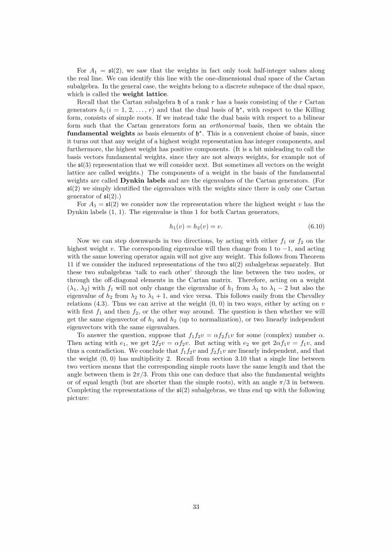
To answer the question, suppose that f1f2v = αf2f1v for some (complex) number α.Then acting with e1, we get 2f2v = αf2v. But acting with e2 we get 2αf1v = f1v, andthus a contradiction. We conclude that f1f2v and f2f1v are linearly independent, and thatthe weight (0, 0) has multiplicity 2. Recall from section 3.10 that a single line betweentwo vertices means that the corresponding simple roots have the same length and that theangle between them is 2π/3. From this one can deduce that also the fundamental weightsor of equal length (but are shorter than the simple roots), with an angle π/3 in between.Completing the representations of the sl(2) subalgebras, we thus end up with the followingpicture:

33

t (−1, 2) t (1, 1)

t (−1,−1) t (1,−2)

t

t (−2, 1) t (2,−1)t (0, 0)i×

×

(0, 1)

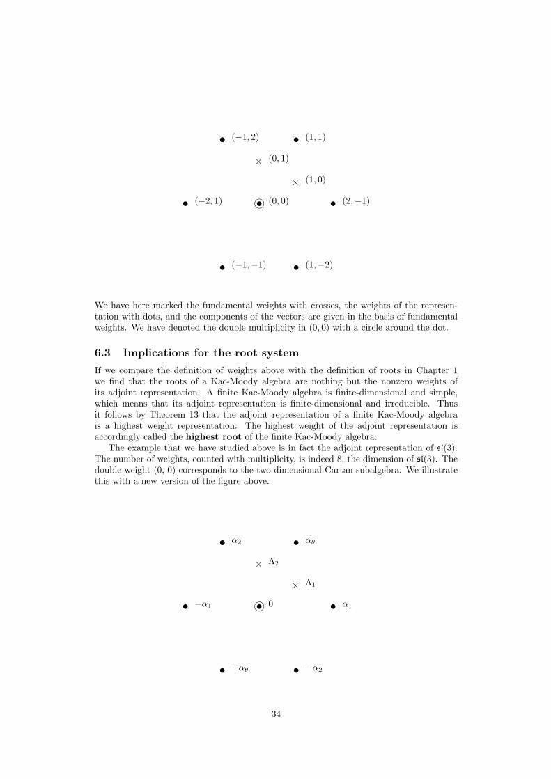
(1, 0)

We have here marked the fundamental weights with crosses, the weights of the represen-tation with dots, and the components of the vectors are given in the basis of fundamentalweights. We have denoted the double multiplicity in (0, 0) with a circle around the dot.

6.3 Implications for the root system

If we compare the definition of weights above with the definition of roots in Chapter 1we find that the roots of a Kac-Moody algebra are nothing but the nonzero weights ofits adjoint representation. A finite Kac-Moody algebra is finite-dimensional and simple,which means that its adjoint representation is finite-dimensional and irreducible. Thusit follows by Theorem 13 that the adjoint representation of a finite Kac-Moody algebrais a highest weight representation. The highest weight of the adjoint representation isaccordingly called the highest root of the finite Kac-Moody algebra.

The example that we have studied above is in fact the adjoint representation of sl(3).The number of weights, counted with multiplicity, is indeed 8, the dimension of sl(3). Thedouble weight (0, 0) corresponds to the two-dimensional Cartan subalgebra. We illustratethis with a new version of the figure above.

t α2 t αθ

t −αθ t −α2

t

t −α1 t α1t 0i×

×

Λ2

Λ1

34

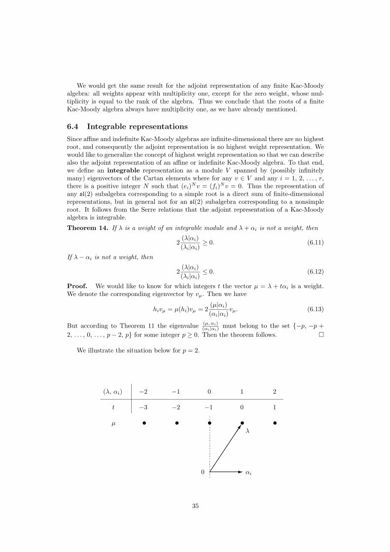
We would get the same result for the adjoint representation of any finite Kac-Moodyalgebra: all weights appear with multiplicity one, except for the zero weight, whose mul-tiplicity is equal to the rank of the algebra. Thus we conclude that the roots of a finiteKac-Moody algebra always have multiplicity one, as we have already mentioned.

6.4 Integrable representations

Since affine and indefinite Kac-Moody algebras are infinite-dimensional there are no highestroot, and consequently the adjoint representation is no highest weight representation. Wewould like to generalize the concept of highest weight representation so that we can describealso the adjoint representation of an affine or indefinite Kac-Moody algebra. To that end,we define an integrable representation as a module V spanned by (possibly infinitelymany) eigenvectors of the Cartan elements where for any v ∈ V and any i = 1, 2, . . . , r,there is a positive integer N such that (ei)Nv = (fi)Nv = 0. Thus the representation ofany sl(2) subalgebra corresponding to a simple root is a direct sum of finite-dimensionalrepresentations, but in general not for an sl(2) subalgebra corresponding to a nonsimpleroot. It follows from the Serre relations that the adjoint representation of a Kac-Moodyalgebra is integrable.

Theorem 14. If λ is a weight of an integrable module and λ+ αi is not a weight, then

2(λ|αi)(λi|αi)

≥ 0. (6.11)

If λ− αi is not a weight, then

2(λ|αi)(λi|αi)

≤ 0. (6.12)

Proof. We would like to know for which integers t the vector µ = λ + tαi is a weight.We denote the corresponding eigenvector by vµ. Then we have

hivµ = µ(hi)vµ = 2(µ|αi)(αi|αi)

vµ. (6.13)

But according to Theorem 11 the eigenvalue (µ, αi)(αi|αi) must belong to the set {−p, −p +

2, . . . , 0, . . . , p− 2, p} for some integer p ≥ 0. Then the theorem follows. �

We illustrate the situation below for p = 2.

t t t t t

�

-0 αi

λµ

t

−2 −1 0 1 2(λ, αi)

−3 −2 −1 0 1

35

6.5 The Weyl group

One important consequence of the theorem in the previous subsection is the followingcorollary:

Theorem 15. If λ is a root and αi is a simple root, then

λ− 2(λ|αi)(αi|αi)

αi (6.14)

is a root as well, with the same multiplicity as λ.

For any root α, define the reflection with respect to α by

λ 7→ λ− 2(λ|α)(α|α)

α (6.15)

This is a reflection in the plane perpendicular to the root α. The corollary thus says thatthe root system, and the root multiplicities, are preserved under the reflections with respectto the simple roots. Such reflections are called fundamental Weyl reflections. Whenα = αi we denote the fundamental Weyl reflection (6.14) by ri.

Whenever some object is invariant under some operations, it is also invariant underthe composition of the two such operations, and therefore it is interesting to study alloperations that can obtained in this way, by successive compositions. In this case we areinterested in the group generated by the fundamental Weyl reflections. This group is calledthe Weyl group, and it is a discrete subgroup of GL(h). Thus the root system, and theroot multiplicities, are preserved under the Weyl group, which means that it is a subgroupto the permutation group of the roots. When the Kac-Moody algebra is finite, the Weylgroup is also finite as a group, since there are only finitely many roots to permute.

Given any two elements of a group, it is of interest to know whether they commute ornot. For the generators of the Weyl group we want to compare rirj and rjri. Since thegenerators are reflections, each of them is its own inverse, riri = 1. Thus we have

rirj = (rjrj)rirj(riri) = rj(rjri)2ri (6.16)

and we see that rirj = rjri if and only if (rjri)2 = 1.When (rirj)2 6= 1, so that rirj 6= rjri, one can ask if there is any integer m ≥ 2 such

that (rirj)m = 1. Let us therefore study (rirj)m for a general integer m ≥ 2. The vectorspace h? is the direct sum of the plane spanned by αi, αj and its orthogonal complement.The orthogonal complement is invariant under both ri and rj , so it is enough to study theplane spanned by αi, αj . In this basis, the matrix realization of ri and rj are

ri =(−1 −Aji0 1

), ri =

(1 0−Aij −1

), rirj =

(−1 +AijAji Aji−Aij −1

), (6.17)

Set M = rirj . Now we invoke the Cayley-Hamilton theorem, which says that a matrixsatisfies its own characteristic equation. We have

det (M − λ1) = λ2 + (2−AijAji)λ+ 1 (6.18)

and so we get

M2 = (AijAji − 2)M − 1. (6.19)

36

Multiplying the equation (6.19) successively with M , and inserting it into the result, weobtain the equation

Mm = amM − am−11 (6.20)

where

am = (AijAji − 2)am−1 − am−2, a0 = 0, a1 = 1. (6.21)

For AijAji−2 ≥ 2 this sequence is increasing, and therefore there is no integer m > 0 suchthat am = 0 which is a necessary condition for Mm = 1. It is conventional to set m =∞in this case, M∞ = 1. In the other cases, 0 ≤ AijAji ≤ 3, one can easily check that m isgiven by the following table:

AijAji 0 1 2 3 ≥ 4mij 2 3 4 6 ∞ (6.22)

Any group that is generated by a finite number n of generators ri (i = 1, 2, . . . , n) modulothe relations (rirj)mij = 1, for arbitrary integers mij = mji ≥ 2, is called a Coxetergroup. When the integers mij are restricted to the values 2, 3, 4, 6 and ∞ as above, thegroup is said to be a crystallographic Coxeter group. The conclusion of this last sectionis thus that the Weyl group of a Kac-Moody algebra is always a crystallographic Coxetergroup. Conversely, any crystallographic Coxeter group is the Weyl group of a Kac-Moodyalgebra, but this is not uniquely given, as can be seen by (6.22). For further readingabout Coxeter groups and the related reflection groups, we recommend the book [?] byHumphreys.

37