LIDAR QC Report - Alaska

OLC Alaska DNR Whittier Acceptance Report.

of 15

Department of Geology & Mineral Industries 800 NE Oregon St, Suite 965

Portland, OR 97232

Alaska DNR LIDAR Project, 2012 – Whittier QC Analysis

LIDAR QC Report – January 14th, 2013

Figure 1. Map featuring Alaska DNR Whittier data extent.

OR

EG

ON

DE

PA

RT

ME NT

O F G E O L O G Y A N DM

I NE

RA

LI N

DU

ST

RIE

S

1937


of 15

The Alaska Department of Natural Resources, Division of Geological and Geophysical

Survey (DGGS) has contracted with Watershed Sciences, Inc (WSI) to collect high resolution lidar topographic data for a study area known as the Whittier Area (Figure 1). DGGS has specified the exact area of data collection as well as a detailed description of data products to be delivered. The complete lidar specifications and deliverables are detailed in Agency Contract No. 10-12-063 signed by DGGS and WSI.

The Oregon Department of Geology and Mineral Industries has contracted with DGGS to provide independent quality control review of aspects of the data provided by WSI. The details of the QC agreement are spelled out in the State of Alaska Cooperative Agreement Number MI-11-006. The primary quality control tasks are:

1. Review and test all delivered files for completeness, correct naming and usability. 2. Evaluate consistency of data by comparing points from the overlapping areas of

adjacent swaths. 3. Visual inspection of images derived from the lidar bare earth and highest hit DEMs to

identify artifacts, voids and missed ground. 4. Test the accuracy of the bare earth DEMs by comparing them to GPS ground control

points provided by DGGS. For each delivery of data, DOGAMI shall prepare a report to DGGS describing the results of the quality control review for that delivery. This is the report for the Whittier LiDAR Project (Figure 1). Upon receipt from vendor (Watershed Sciences), all lidar data for the Whittier Project were

independently reviewed by staff from the Oregon Department of Geology and Mineral Industries (DOGAMI) to ensure project specifications were met. The entire delivery consisted of the following data products:

• Bare Earth Hydro flattened Grids: Tin interpolated raster grids created from lidar ground returns. All lake and large water bodies are “flattened” to create a uniform water surface.

• Highest Hit Grids: Tin interpolated raster grids created from the highest lidar elevation for a given 1 meter cell.

• Intensity TIF: TIF raster built using returned lidar pulse intensity values gathered from highest hit returns.

• Vegetation Grids: Interpolated raster grids with values representing height above bare earth.

• Trajectory File: File contains point location measurement of the aircraft used to collect lidar data. Data is collected using an Inertial Measurement Unit (IMU), and collects measurements of: Easting(meters), Northing (meters), Ellipsoid Height (meters) of aircraft, aircraft roll (degrees), aircraft pitch (degrees), aircraft heading (degrees). Measurements are collected at one second intervals.

• LAS: Binary file of all lidar points collected in survey (Class, flight line #, GPS Time, Echo, Easting, Northing, Elevation, Intensity, Scan Angle, Echo Number, and Scanner).

• Raw LAS by Flight line: Unclassified lidar point data in las format. Data is organized by flight line.


of 15

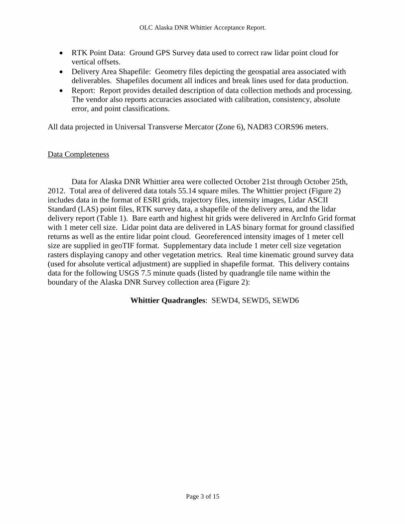
• RTK Point Data: Ground GPS Survey data used to correct raw lidar point cloud for vertical offsets.

• Delivery Area Shapefile: Geometry files depicting the geospatial area associated with deliverables. Shapefiles document all indices and break lines used for data production.

• Report: Report provides detailed description of data collection methods and processing. The vendor also reports accuracies associated with calibration, consistency, absolute error, and point classifications.

All data projected in Universal Transverse Mercator (Zone 6), NAD83 CORS96 meters.

Data Completeness

Data for Alaska DNR Whittier area were collected October 21st through October 25th,

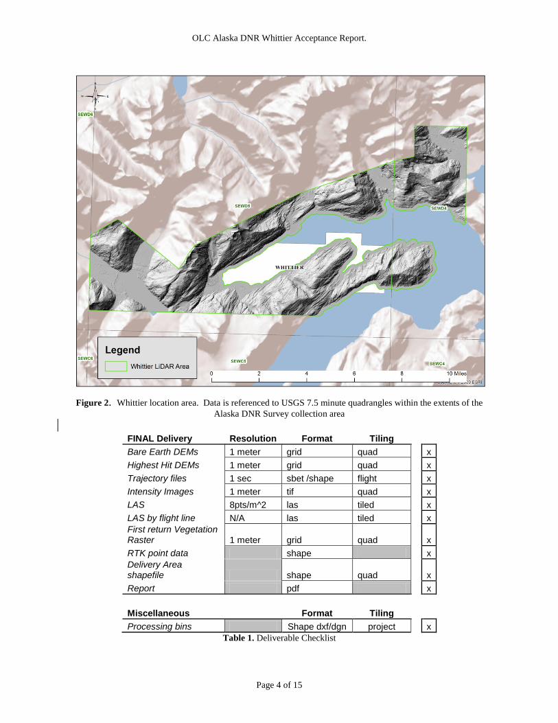
2012. Total area of delivered data totals 55.14 square miles. The Whittier project (Figure 2) includes data in the format of ESRI grids, trajectory files, intensity images, Lidar ASCII Standard (LAS) point files, RTK survey data, a shapefile of the delivery area, and the lidar delivery report (Table 1). Bare earth and highest hit grids were delivered in ArcInfo Grid format with 1 meter cell size. Lidar point data are delivered in LAS binary format for ground classified returns as well as the entire lidar point cloud. Georeferenced intensity images of 1 meter cell size are supplied in geoTIF format. Supplementary data include 1 meter cell size vegetation rasters displaying canopy and other vegetation metrics. Real time kinematic ground survey data (used for absolute vertical adjustment) are supplied in shapefile format. This delivery contains data for the following USGS 7.5 minute quads (listed by quadrangle tile name within the boundary of the Alaska DNR Survey collection area (Figure 2):

Whittier Quadrangles: SEWD4, SEWD5, SEWD6


of 15

Figure 2. Whittier location area. Data is referenced to USGS 7.5 minute quadrangles within the extents of the

Alaska DNR Survey collection area

FINAL Delivery Resolution Format Tiling Bare Earth DEMs 1 meter grid quad x Highest Hit DEMs 1 meter grid quad x Trajectory files 1 sec sbet /shape flight x Intensity Images 1 meter tif quad x LAS 8pts/m^2 las tiled x LAS by flight line N/A las tiled x First return Vegetation Raster 1 meter grid quad x RTK point data shape x Delivery Area shapefile shape quad x Report pdf x Miscellaneous Format Tiling Processing bins Shape dxf/dgn project x

Table 1. Deliverable Checklist


of 15

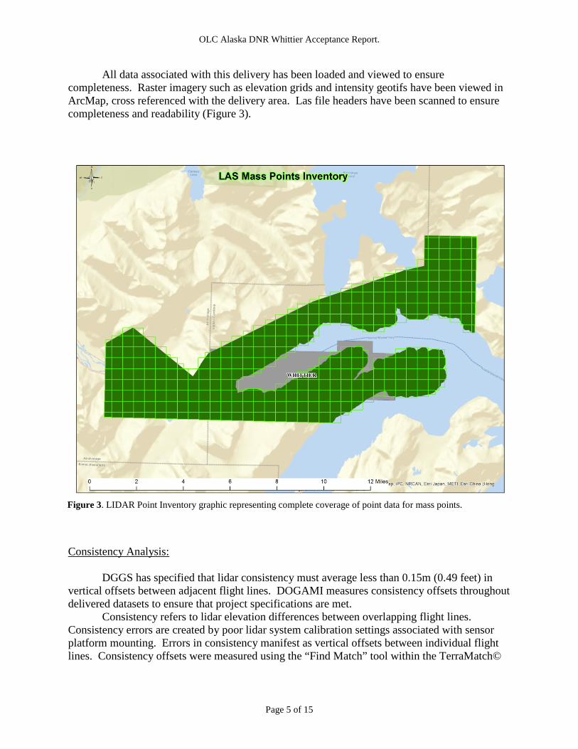
All data associated with this delivery has been loaded and viewed to ensure completeness. Raster imagery such as elevation grids and intensity geotifs have been viewed in ArcMap, cross referenced with the delivery area. Las file headers have been scanned to ensure completeness and readability (Figure 3).

Figure 3. LIDAR Point Inventory graphic representing complete coverage of point data for mass points. Consistency Analysis:

DGGS has specified that lidar consistency must average less than 0.15m (0.49 feet) in vertical offsets between adjacent flight lines. DOGAMI measures consistency offsets throughout delivered datasets to ensure that project specifications are met.

Consistency refers to lidar elevation differences between overlapping flight lines. Consistency errors are created by poor lidar system calibration settings associated with sensor platform mounting. Errors in consistency manifest as vertical offsets between individual flight lines. Consistency offsets were measured using the “Find Match” tool within the TerraMatch©


of 15

software toolset. This tool uses aircraft trajectory information linked to the lidar point cloud to quantify flight line-to-flight line offsets.

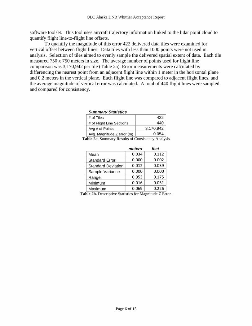
To quantify the magnitude of this error 422 delivered data tiles were examined for vertical offset between flight lines. Data tiles with less than 1000 points were not used in analysis. Selection of tiles aimed to evenly sample the delivered spatial extent of data. Each tile measured 750 x 750 meters in size. The average number of points used for flight line comparison was 3,170,942 per tile (Table 2a). Error measurements were calculated by differencing the nearest point from an adjacent flight line within 1 meter in the horizontal plane and 0.2 meters in the vertical plane. Each flight line was compared to adjacent flight lines, and the average magnitude of vertical error was calculated. A total of 440 flight lines were sampled and compared for consistency.

Summary Statistics # of Tiles 422 # of Flight Line Sections 440 Avg # of Points 3,170,942 Avg. Magnitude Z error (m) 0.054

Table 2a. Summary Results of Consistency Analysis

meters feet Mean 0.034 0.112 Standard Error 0.000 0.002 Standard Deviation 0.012 0.039 Sample Variance 0.000 0.000 Range 0.053 0.175 Minimum 0.016 0.051 Maximum 0.069 0.226

Table 2b. Descriptive Statistics for Magnitude Z Error.


of 15

Figure 4. Histogram of flight line offsets values.

Results of the consistency analysis found the average flight line offset to be 0.054 meters with a maximum error of 0.095m (Table 2b). Distribution of error showed over 97% of all error was less than 0.07m (Figure 4). The highest 3% of error occurs in areas of steep terrain and is a result of slope. These results show that all data are within tolerances of data consistency according to contract agreement.

0%

10%

20%

30%

40%

50%

60%

70%

80%

90%

100%

0

50

100

150

200

250

300

0.01 0.02 0.03 0.04 0.05 0.06 0.07 0.08 0.09 0.10 More

Freq

uenc

y

Absolute Vertical Offset (meters)

Frequency Histogram of Absolute Error Associated with Flightline Consistency

Frequency

Cumulative %


of 15

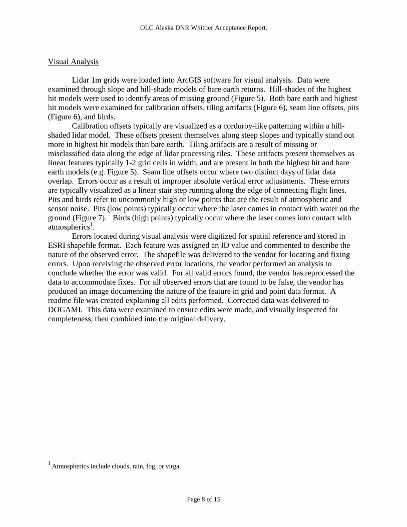
Visual Analysis

Lidar 1m grids were loaded into ArcGIS software for visual analysis. Data were examined through slope and hill-shade models of bare earth returns. Hill-shades of the highest hit models were used to identify areas of missing ground (Figure 5). Both bare earth and highest hit models were examined for calibration offsets, tiling artifacts (Figure 6), seam line offsets, pits (Figure 6), and birds.

Calibration offsets typically are visualized as a corduroy-like patterning within a hill-shaded lidar model. These offsets present themselves along steep slopes and typically stand out more in highest hit models than bare earth. Tiling artifacts are a result of missing or misclassified data along the edge of lidar processing tiles. These artifacts present themselves as linear features typically 1-2 grid cells in width, and are present in both the highest hit and bare earth models (e.g. Figure 5). Seam line offsets occur where two distinct days of lidar data overlap. Errors occur as a result of improper absolute vertical error adjustments. These errors are typically visualized as a linear stair step running along the edge of connecting flight lines. Pits and birds refer to uncommonly high or low points that are the result of atmospheric and sensor noise. Pits (low points) typically occur where the laser comes in contact with water on the ground (Figure 7). Birds (high points) typically occur where the laser comes into contact with atmospherics1.

Errors located during visual analysis were digitized for spatial reference and stored in ESRI shapefile format. Each feature was assigned an ID value and commented to describe the nature of the observed error. The shapefile was delivered to the vendor for locating and fixing errors. Upon receiving the observed error locations, the vendor performed an analysis to conclude whether the error was valid. For all valid errors found, the vendor has reprocessed the data to accommodate fixes. For all observed errors that are found to be false, the vendor has produced an image documenting the nature of the feature in grid and point data format. A readme file was created explaining all edits performed. Corrected data was delivered to DOGAMI. This data were examined to ensure edits were made, and visually inspected for completeness, then combined into the original delivery.

1 Atmospherics include clouds, rain, fog, or virga.


of 15

Figure 5. Example of missing ground in lidar bare earth data. Ground is clearly visible in highest hit model, but has been removed from the bare earth model. This type of classification error is common near water body features.


of 15

Figure 6. Example of tile artifact found in highest hit lidar data. Artifact is a seam line error created due to misclassification of ground at edge of lidar processing tiles.


of 15

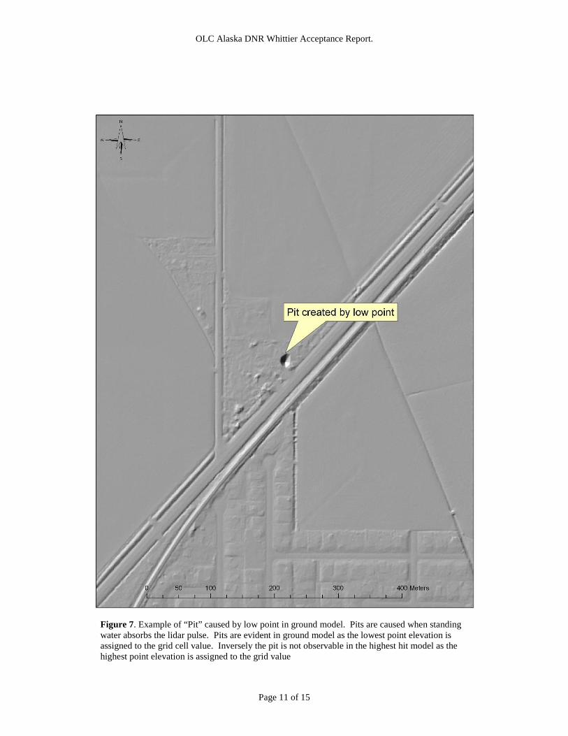
Figure 7. Example of “Pit” caused by low point in ground model. Pits are caused when standing water absorbs the lidar pulse. Pits are evident in ground model as the lowest point elevation is assigned to the grid cell value. Inversely the pit is not observable in the highest hit model as the highest point elevation is assigned to the grid value


of 15

Absolute Accuracy Analysis:

Absolute accuracy refers to the vertical offset of lidar data relative to measured ground-control points (GCP) obtained throughout the lidar sampling area. The contractor used a surveying system (Figure 8) to measure GCP’s. GPS survey techniques allow surveyors to collect many precisely located GCP's which can be used as a control comparison with LiDAR elevations. For example, Trimble reports that the 5700/5800 GPS system have horizontal errors of approximately ±1-cm + 1ppm (parts per million * the baseline length) and ±2-cm in the vertical (TrimbleNavigationSystem, 2005). A licensed surveyor is often able to post process GPS survey data to accuracies less than 1cm in both horizontal and vertical axes.

Figure 8. The Trimble 5700 base station antenna located over a known reference point at Cove Oregon. Corrected GPS position and elevation information is then transmitted by a Trimmark III base radio to the 5800 GPS rover unit.

Vertical accuracy analysis consisted of differencing control data and the delivered lidar

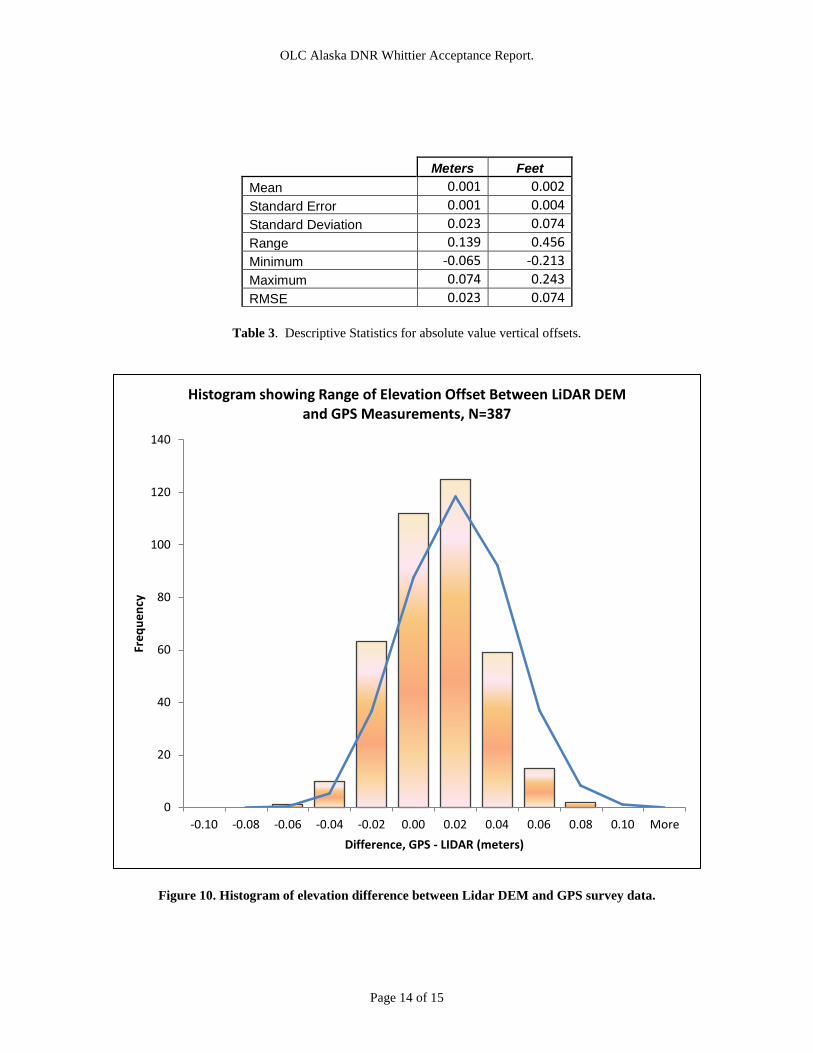
Digital Elevation Models (DEM) to expose offsets. These offsets were used to produce a mean vertical error and vertical RMSE values for the entire delivered data set. Project specifications list the maximum acceptable root mean square vertical offset to be 0.20 meters (0.65 feet). A total of 387 measured GCP’s were provided to DOGAMI by DGGS for the Whittier Project Area (Figure 9) and compared with the lidar elevation grids. The data delivered to DOGAMI was found to have a mean vertical offset of 0.001 meters (0.002 feet) and an RMSE value of 0.023 meters (0.074 ft). Offset values ranged from -0.065 to 0.074 meters (Table 3 and Figure 10). Horizontal accuracies were not specified in agreement since true horizontal accuracy is regarded as a product of the lidar ground foot print. Lidar is referenced to co-acquired GPS base station data that has accuracies far greater than the value of the lidar foot print. The ground footprint is equal to 1/3333rd of above ground flying height. Survey altitude for this acquisition was targeted at 900 meters yielding a ground foot print of 0.27 meters. This value exceeds the typical accuracy value of ground control used to reference the lidar data (<0.01m). Project specifications require the lidar foot print to fall within 0.15 and 0.40 meters.


of 15

Figure 9. Locations of RTK control surveyed by Contractor. Data was used to test absolute accuracy for

the Alaska DNR lidar survey within the Whittier project extent.


of 15

Meters Feet Mean 0.001 0.002 Standard Error 0.001 0.004 Standard Deviation 0.023 0.074 Range 0.139 0.456 Minimum -0.065 -0.213 Maximum 0.074 0.243 RMSE 0.023 0.074

Table 3. Descriptive Statistics for absolute value vertical offsets.

Figure 10. Histogram of elevation difference between Lidar DEM and GPS survey data.

0

20

40

60

80

100

120

140

-0.10 -0.08 -0.06 -0.04 -0.02 0.00 0.02 0.04 0.06 0.08 0.10 More

Freq

uenc

y

Difference, GPS - LIDAR (meters)

Histogram showing Range of Elevation Offset Between LiDAR DEM and GPS Measurements, N=387

LIDAR QC Report - Alaska

Documents

Transcript of LIDAR QC Report - Alaska