LIBRARY

FTS THESIS 629.252 COS 30001007614367 Cosic, Ivan Development and testing of a variable valve timing system (VVT) for a twincam

ACKNOWLEDGEMENT

I would like to gratefully thank m y supervisor, Kevin Hunt and m y co-supervisor

Mark Armstrong for their valuable guidance, patience and advice. Without their

support this project would not have been possible.

I am grateful to Professor Geoffrey Lleonart for his patience and advice in the

correction of m y thesis.

I wish to thank the technical staff at the School of Built Environment, especially

Laurance Martin and Harry Friedrich for constructing the cylinder head test rig and

practical assistance.

I wish to thank Bruce Cameron from Holden Australia for his kind donation of a

Holden Vectra 2.0 litre twincam engine for the project.

I am thankful to MSC Software for their support and advice in ADAMS software.

Finally, I would like to thank my entire family for their support.

ii

TABLE OF CONTENTS

ABSTRACT

1. INTRODUCTION

1.1 Background

1.3 Aim

2.1 Introduction

2.2 Phase Changing

1.2 Variable Valve Timing 3

4

1.4 Approach 4

2. LITERATURE REVIEW 5

5

5

2.3 Cam Changing 10

2.4 Intake Valve Closing !5

2.5 Lost Motion Valves 18

2.6 Electrically Actuated Valves 19

2.7 Hydraulically Actuated Valves 20

2.8 Valves Actuated by Two Cams in Parallel 21

2.9 Literature Review Summary 22

3. METHODS AND EQUIPMENT 23

3.1 Introduction 23

3.2 Engine Specification 23

3.3 Cylinder Head Test Rig 24

3.4 Laser Displacement Sensor 25

3.5 DTVEE Software 2 8

iii

3.6 Vectra Engine Cylinder Head Valve Profile

3.7 Hertzian Contact Theory 30

4. RESULTS AND DISCUSSION 33

33

33

39

47

4.1 Computer Simulation

4.2 DVC Components

4.2.1 Constraints

4.3 Dynamic Valve Control

4.4 Simulation Results

4.4.1 DVC Valve Profile 52

4.4.2 Valve Velocity and Acceleration Results 69

4.5 Force and Stress Analysis of Components 81

4.5.1 Forces Acting on DVC Components 82

4.5.2 Stress Analysis 93

4.5.3 Hertz Contact Pressure "

5. CONCLUSIONS AND RECOMMENDATIONS 100

5.1 Conclusions 10°

101 5.2 Recommendations

6. REFERENCES

APPENDIX A

APPENDIX B

APPENDIX C

102

107

111

112

iv

ABSTRACT

Variable valve timing ( W T ) is an innovative design that enhances automotive engine

performance and is important in addressing fuel consumption and emission output

concerns. The purpose of the research reported here was to examine the concept of a

W T system because it had the promise of application in the advancement of engine

technology.

In this study, a new WT system, termed the dynamic valve control (DVC) system

was developed. The D V C system was modeled using the computer simulation

software package A D A M S , which determined the forces acting on the principal

components at operational speeds, as well as the valve timing and lift profile of the

system. Stress analysis of the rocker arm was carried out using Cosmos/DesignStar

software. The valve timing and lift characteristics of the D V C system were compared

to an existing standard production engine.

The results of the study showed that the proposed DVC system can essentially realise

closure of its valves and achieve variable valve lift. In addition, the D V C system

valve timing and lift profile showed better characteristics when compared with those

of an existing Holden Vectra 2.0 litre twincam engine.

v

1. INTRODUCTION

1.1 Background

Resources of fossil fuels are finite and if they are to be used to provide energy for transport

they must be used efficiently. There are also strong pressures to make automotive vehicles

less environmentally polluting and one of the most important factors in reducing global

warming is the increased use of vehicles with better fuel economy. The U.S Department of

Energy (1998) concluded that for every litre of fuel burnt in a vehicle, 9 kilograms of carbon

dioxide, a greenhouse gas pollutant, is transferred into the atmosphere. By choosing a vehicle

with a fuel consumption of 50 kilometres rather than 40 kilometres per litre can prevent

approximately 10000 kilograms of carbon dioxide from being released over the lifetime of a

vehicle.

About 15% of the energy in the fuel is used to propel a vehicle, the rest of the energy is lost

to atmosphere. Automobiles need energy to accelerate, and to overcome air resistance and

the friction from tires, wheels and axles. Fuel provides the needed energy in the form of

chemicals that can be combusted to release heat. Engines transform heat released in

combustion into useful work that ultimately turns the vehicle wheels, propelling it along the

road, see U.S Department of Energy (2001).

Over the last decade there has been a significant improvement in the fuel consumption of

vehicles and as a result they have become less polluting. The most effective way to increase

horsepower and /or efficiency is to increase an engine's ability to process air. Since the

engine valves play a major role in controlling the flow of air/fuel mixture into and out of the

cylinders, it is important to study the role of engine valve systems in relation to improving

the efficiency of automotive engines.

Valves activate the airflow of an automotive engine. The timing of air-intake and exhaust is

controlled by the shape and phase angle of cams. To optimise the air-flow, engines require

different valve timings at different speeds, and it has been found beneficial to open the inlet

valve earlier and close the exhaust valve later. In other words, the overlapping between the

1

intake and exhaust periods should be increased as the engine speed increases.

Overlap refers to the period when both the intake and exhaust valves are open at the

same time. W h e n the intake valve is opened before the exhaust valve closes, a scavenging

effect occurs, in which the rush of the exhaust out of the cylinder draws in a little more of the

intake charge into the cylinder.

The valves of an engine do not open and close exactly when the piston reaches the top and

bottom of its cycle. The intake valve begins to open before the piston reaches top dead centre

(TDC), and closes after the piston reaches bottom dead centre (BDC). The exhaust valve

begins to open as the piston reaches the bottom, and begins to close as the piston reaches the

top. As the engine's speed increases, air in the manifold gains momentum, and even when

the piston reaches B D C , air continues to be drawn into the cylinder. Thus, to obtain as much

air as possible in the cylinder without causing inefficiencies from inertial forces, it is

desirable to have the valve timing change with the engine speed.

Previously, manufacturers have used one or more camshafts to open and close an engine's

valves. The camshaft is turned by a timing chain connected to the crankshaft and as the

engine speed increases or decreases, the crankshaft and camshaft rotate to keep the valve

timing close to that needed for engine operation. Increased valve duration (the length of time

that the valves are held open) yields greater power at high speed but reduces torque at low

speed. While a greater valve lift (distance that the valves are opened, usually expressed in

millimetres) without increasing duration, yields more power without much change in the

nature of the power curve. Generally it is impractical to optimise the valve timing for both

high and low engine speed with a simple crankshaft-driven valve train. As a result, engine

designers have to compromise timing in the specification of the camshaft. For example, an

ordinary sedan has its valve timing optimized for mid-range engine speed so that both low

speed driving ability and high-speed output do not significantly suffer. However, this

compromise results in wasted fuel and reduced performance beyond the optimized speed

range, see Brauer (1999).

2

1.2 Variable Valve Timing

As technology has advanced, so too has the development of engine design and nowadays it is

normal for modern vehicles to have multi-valve technology. Variable valve timing ( W T ) is

seen as the next step to enhance engine efficiency.

Variable valve timing was first introduced as an innovative design that increased engine

torque and output while addressing environmental issues, such as pollutants emitted from

automotive engines. The variable valve timing system uses an electronic system, known as

the engine control unit (ECU) to electronically control the operation of the engine valves.

The system is able to detect the engine speed and adjust the valve timing accordingly. As a

consequence, more oxygen can be supplied through the air intake valve as more fuel is

injected into the combustion chamber. Greater fuel and oxygen in the combustion chamber

leads to increased power and torque.

Most variable valve timing systems are combined with lift control, which varies the lift of the

intake and exhaust valves while the engine is operating at high speed. As the intake and

exhaust valve lift increases, a larger volume of air/fuel mixture is introduced, along with

ejection of a greater volume of exhaust gas. This results in the engine producing higher

output power while operating at high speeds. The variable valve timing system allows the

valve timing of an automotive engine to be ideally fixed by increasing the valve lift when the

engine speed is high, which results in improved fuel economy.

In principle, variable valve timing improves fuel efficiency and performance because it

adjusts the valve timing between high and low engine speeds for optimum performance, thus

efficiency throughout the entire speed range can be improved.

The variable valve timing system proposed in this study called the dynamic valve control

system ( D V C ) is a unique system based on the concept of varying the degree of valve lift, the

duration of valve opening and capable of virtual closure of the valves.

3

1.3 Aim

The aim of the research program reported here was to develop a computer based model of a

variable valve timing system, developed by m y co-supervisor Mark Armstrong, called

dynamic valve control (DVC) for automotive engines.

1.4 Approach

The present study represents the initial stage of a research and development program

involving the design and construction on an experimental D V C system to be fitted to an

existing automotive engine.

To achieve this aim a computer simulation model showing the operation of the DVC system

was constructed using A D A M S software. This virtual model was used to establish a

geometry that improves engine performance. The forces acting on the rocker arm of the D V C

system were analysed, enabling the design of this component to be refined. In addition, the

valve timing and lift characteristics of a current production engine were compared to the

D V C system's valve timing sequencing.

4

2. LITERATURE RE\TEW

2.1 Introduction

Many mechanisms have been proposed to produce variable valve timing systems. Each

mechanism varies the valve timing either in duration, phase, or both. There are numerous

versions of W T mechanisms in production today, and these W T systems can be basically

classified into seven W T models, which are reviewed below.

2.2 Phase Changing

Cam phasing WT is the simplest, cheapest and most common mechanism used presently.

Basically, it varies the valve timing by shifting the phase angle of camshafts relative to the

crankshaft. Wilson et al. (1993), concluded that intake and exhaust camshafts can be

simultaneously varied with notable improvements in fuel economy and emission reduction,

this was also confirmed by Ashley (1995).

The phase angle can be shifted either by the use of a phasing actuator, whereby the change in

phase angle is produced by adjusting the hydraulic flows in and out of the actuator chambers

or with the camshaft drive being connected to the camshaft through a helical spline. The

latter mechanism was employed by Maekawa (1989). The phase angle between the

driveshaft and the camshaft was changed as the idler gear was moved axially along the

camshaft or vice-versa.

Wilson et al. concluded that high performance double overhead cam (DOHC) engines had a

long valve open duration, high valve lift and produced maximum power output. However,

the large valve overlap caused poor idle stability and also reduced engine torque at low

speeds.

5

Moriya et al. (1996) developed the Intelligent Variable Valve Timing (WT - I ) , as depicted in

Figure 2.1. The W T - I system varies the valve timing by shifting the phase angle of

camshafts and only responds when the valves open and close in relation to engine speed. It

basically consists of three parts:

Crank Position Engine Oil Pump Sensor

Figure 2.1 - W T - 1 system

(1) WT-I Pulley - Located at the front end of the intake camshaft, it produces a timing

difference between the intake camshaft and the crankshaft by a hydraulic actuator.

(2) Oil Control Valve (OCV) - Controls oil pressure to the WT-I pulley according to ECU

command and continually controlling oil feeding and draining between the W T - I Pulley

and O C V achieves continual phasing.

(3) Engine Control Unit (ECU) - Computes optimal valve timing based on the engine

operating condition and drives the O C V . The O C V control current is determined by

comparing the target advance angle, according to the engine operating condition, with

actual advance angle.

6

Titolo (1991) investigated the use of a Fiat W T system for use in a V 8 engine. The W T

device comprised :

(1) A multi-dimensional cam-follower assembly

(2) An actuator regulator assembly

The multi-dimensional cam follower varies the valve opening/closing, both in phase and in

lifting. The actuator regulator assembly changes the cam-follower position by means of an

axial displacement of the camshaft, which takes place continuously as a function of engine

speed.

When the engine is running, the rotation of the camshaft begins to open the intake or the

exhaust valve. At the beginning of valve opening, an oscillating plate is in a nearly

horizontal position. As the valve lift increases, the plate changes its inclination until it

assumes the maximum inclination at maximum lift. During the valve-closing phase, the

maximum plate inclination returns to a horizontal position.

Steinberg et al. (1998) developed a fully continuous variable camshaft timing (VCT) system

which can be applied to both intake and exhaust camshafts. The V C T system is shown in

Figure 2.2.

7

Figure 2.2 - V C T system

Sensors and triggerwheels are used to measure the camshaft position relative to Top

Dead Centre (TDC). The engine management system processes these data to continuously

control the cam position via an electric current to the solenoid.

A cylindrical component, which has helical gears on its exterior and interior surface, is fitted

between the camshaft pulley and the camshafts end. The gear on the exterior surface meshes

with a corresponding gear in the bore of the camshaft pulley, while the interior gear meshes

with a gear mounted on the end of the camshaft. Opposite the camshaft, a piston is moved

axially by oil pressure depending on the camshaft position. The axial movement is

transformed into a rotation of the camshaft relative to the timing pulley. Leone et al. (1996)

concluded that there were three benefits to the V C T system. Firstly, N O x is reduced due to

the increased internal residual, secondly, unburned Hydrocarbons are reduced because they

were drawn back into the cylinder to be "reburnt" during the next combustion cycle, and

thirdly, the intake stroke pumping work was reduced.

Griffiths et al. (1988) developed their own phase changing WT mechanism called the

8

Mitchell mechanical variable valve timing system. The system exploits angular velocity to

change valve timing.

The system can be seen in Figure 2.3, and it is the eccentricity of the driveshaft axis to the

camshaft axis that generates a change in valve timing by imposing a variable angular velocity

on the camshaft. The variation creates a phase lag and phase lead of the camshaft in relation

to the drive shaft that is exploited to change the valve timing.

Common driveshaft

, I Hollow camshaft L|nk

Figure 2.3 - Mitchell W T system

The Mitchell system can be applied to single or multi-cylinder engines with single or twin

camshaft configurations.

Yagi (1992) et al. developed a variable valve actuation mechanism called the shuttle cam.

The system, shown in Figure 2.4, uses a gear-train-driven valve system with a rocker arm

that activates the valve. The cam gears rotate around the idler gear and the camshafts move

along the rocker-arm surface that are concentric with the idler gear. This enables variation of

lift by the alternation of the rocker-arm lever ratio and the cam phasing changes

simultaneously with the degree of rotation of the cam gears.

9

Figure 2.4 - Shuttle cam

A variable valve timing system called the VAST, was developed by Hannibal et al. (1998),

the system enabled the variable control of the intake and exhaust valves. It was possible to

vary the valve opening, up to approximately 50° crankshaft angle, continuously for each

valve lift movement. As a result, fuel consumption and emissions were reduced.

Cam phasing WT systems, are simple and compact mechanisms that have minimal wear

and energy loss. However to date, they cannot vary the duration of valve opening, thus

allowing only earlier or later valve opening.

2.3 Cam Changing

Cam changing systems are the most efficient WT systems in production presently, since

10

they allow variability in the duration of valve opening as well as the lift of the valves. They

can also switch between completely different cam profiles, unlike other systems which can

only basically vary the timing by advancing and retarding a standard set of cams.

In 1989, Hosaka et al. (1991) introduced the valve timing electronic control (VTEC)

engine system, which was able to maintain a high output throughout the entire engine speed

range. Thus enabling the high speed performance of a racing engine without sacrificing low

and medium speed performance.

Heywood (1988) stated that to develop a high performance engine it is necessary to increase

the volumetric efficiency and reduce friction. A racing engine requires wider valve overlap

and increased valve lift to obtain optimum performance at high engine speed. However in a

conventional engine, the valve timing and degree of valve lift is set for optimum

performance at low and medium engine speeds.

Hosaka et al. (1991) identified that by designing for higher valve lift, wider valve timing and

larger valve diameter, it was possible to obtain a higher volumetric efficiency to cope with

high output engine speeds. With V T E C , the valve timing and lift can be adjusted at low

engine rotation to increase torque and prevent air from being forced back through the intake.

A diagrammatic view of the VTEC system is shown in Figure 2.5. The cam has three

separate profiles located at the intake and exhaust of each cylinder. The centre profile is used

exclusively for high speed and the two identical outside profiles for low speed.

11

® Camshaft ,=.,,. .. „ (Z} Hydraulic Piston A

® Cam Lobe for Low Speed Range ® Hydraulic Piston B

® Cam Lobe for High Speed R a n e e <g, Stopper pjn

9> Primary Rocker Arm @ Lost-motion Spring

® Mid Rocker Arm & E x „ a u s , Va|ye

© Secondary Rocker Arm @ ln,ake Va|ve

Figure 2.5 - V T E C system

The rocker arm assembly comprises a mid rocker arm with primary and secondary rocker

arms on each side. The changeover mechanism is composed of two hydraulic pistons that are

located within the rocker arm, a stopper pin and a return spring. A lost motion spring is

located within the mid-rocker arm, so that the valve can open and close at high speeds. The

whole system is operated by a hydraulic actuator, which is controlled by the engine control

unit (ECU).

The V T E C has a four valve per cylinder valve arrangement. The V T E C camshaft has a low-

speed and high-speed cam profile. While in lower speed mode, the valve timing goes along

with the low-speed cam and once the engine reaches high speed, the outer rocker arm lifts off

12

the low-speed cam and follows the high speed cam. This effectively allows the high-speed

cam to control the two valve timings. Hosaka et al. concluded that since the high-speed cam

was able to control the two valve settings, the engine was able to get sufficient air at both

low and high speeds. As a result, the engine was able to perform better with an even torque

band, and more than adequate power at the high end.

Matsuki et al. (1996) conducted further research of the VTEC system by developing a three

stage V T E C lean burn engine. The mechanism developed was based on the previous V T E C

system but included modifications to the valve train, intake port and combustion chamber

configurations. The three-stage V T E C system had the same the valve timing and lift

switching mechanism as its predecessor, the V T E C .

As illustrated in Figure 2.6, it can be seen that the three stage VTEC system's camshaft has

three cam lobes per valve pair and rocker arms for primary, secondary and middle cam

profiles. The three profiles are for valve inactivity, low and medium engine speeds and high

engine speed. The rocker arm integrates two hydraulic passages, which can be switched to

and from each other by a spool valve setting.

Medium-speed switching piston

High speed switching piston

Y Medium-speedcam

\ High-speed cam

Inactive cam

Figure 2.6 - 3-Stage V T E C system

13

At medium-speed range, the hydraulic passage opens as a result of the electronic control unit

(ECU) signal, providing hydraulic pressure to the switching piston. The primary and

secondary rocker arms are connected to each other and lift the valve using the medium-speed

cam profile. The valve timing and lift at this stage are set so that they ensure an appropriate

charging efficiency and less valve drive friction.

While in the high-speed range, the ECU allows the other hydraulic passage to open,

providing hydraulic pressure to the high-speed switching piston. As a result, both the primary

and secondary rocker arms are connected to the middle rocker arm. Consequently accessing

the high-speed cam profile, the valve timing and lift are optimized to generate a high power

output.

They concluded that the three-stage VTEC system can generate approximately 40% more

engine power than the original V T E C engine that Hosaka et al. (1991) developed, while

maintaining the same fuel consumption. Nakayame et al. (1994) concluded that because the

V T E C systems alter the valve timing and lift according to various driving conditions, it was

able to use a leaner mixture than existing engines. As a result, the V T E C systems reduce

Hydrocarbon emissions considerably due to the improvement in engine combustion.

Hatano et al. (1993), developed a WT system featuring a multi-mode valve system, it was

called Mitsubishi Innovative Valve Timing and Lift Electronic Control (MTVEC). The

system enables deactivation of unnecessary cylinders during low speed cruise and improved

the engine output performance under all engine speed ranges by selecting optimum cam

profiles depending on the engine speed, as shown in Table 2.1

14

0 ACTIVATED • DEACTIVATED

MODE

I

I I

CYLINDER

NO. 1,4 CYUNDERSH

NO. 1,3 CYUNDEfli.

ALL CYLINDERS

ALL CYLINDERS

CAM FOLLOWER

LOW. SPEED CAM HIGH • SPEED CAW

•

0 0 .-*. •

•

t •

0

Table 2.1 - M I V E C valve operation

Hara and Kumaga (1989) developed a WT lift and timing control system (VLTC), which

varied the lift timing by changing the fulcrum of the rocker arm. The fulcrum was varied

according to the inclination of a lever that engages with a control cam. The control cam was

driven by an actuator mechanism to provide control over valve lift and timing. They

concluded that their system reduced valve train noise and delivered stable valve operation

throughout the high-speed range.

Although cam changing WT systems can vary the lift of the valves, they cannot fully close

the valves to zero lift, as well, additional cams are required to vary the lift from low-speed to

high-speed.

2.4 Intake Valve Closing

Intake valve closing is a practical concept applicable to engines in which the intake valves

can be phased relative to each other to extend the total intake opening period. Bassett et al.

(1997) studied the use of a late intake valve closing (LIVC) mechanism as a means to

15

eliminate most of the pumping losses (pumping loss represents the power required to pump

charge into and out of the cylinders) and conserve fuel. They identified that the problem of

pumping losses must be addressed, because as the engine was throttled, pumping losses

progressively increased until no useful output was generated at idle speed.

Their proposed system consists of an intake camshaft, which causes late closing of the intake

valve at all times. At high loads a reed valve situated in the intake manifold prevented the

charge from being rejected from the cylinder. At low loads, the reed valve was deactivated to

allow the charge to return to the inlet manifold. They asserted that the LrVC system allowed

the engine to operate with wider than normal throttle settings at low speed, thus enabling the

reduction of pumping losses.

Ma (1988) and Saunders et al. (1989) agreed with Bassett's research by also concluding that

there was better fuel consumption with the LIVC. Lenz and Wichart (1989) stated that with a

late intake valve closing mechanism, a torque increase of 8 % can be achieved, fuel

consumption can be improved by 4 % , along with and a 2 0 % - 5 0 % reduction in pumping

losses.

Payri et al. (1984) compared pumping losses between a standard engine and an engine fitted

with a W T system. Their conclusion was that pumping losses would be significantly

reduced with a W T system and the efficiency of an engine would improve. They found that

there was a strong pressure drop in the throttle valve of the carburetor when the engine runs

at a partial load rate, this decreased the mean pressure along the intake and as a result,

pumping losses were increased. With a W T system, the throttle valve was eliminated and

load regulation was achieved by means of the total opening time of the intake valve. The

pressure drop during the intake process was minimal and the fluid inside the cylinder

expands from the moment that the intake valve was closed until the piston reached bottom

dead centre (BDC) and afterwards was compressed during the compression stroke.

On the other hand, Tuttle (1982) investigated the use of an early intake valve closing (EIVC)

mechanism as a means for controlling the load of a spark-ignition engine. The engine was

operated unthrottled, with load controlled by closing the intake valve during the intake stroke

16

of the engine after the required amount of charge has been induced into the cylinder. H e

found that compared to a conventional throttled engine operating at part load, the EIVC

had lower pumping loss, fuel consumption and N O x emissions. O n the other hand, Hara et al.

(1989) found that even though pumping losses were reduced with intake valve closing

mechanisms, improvement in fuel economy equivalent to the reduction in pumping losses

were not obtained. They concluded that the major contributing factor to this phenomenon

was the deterioration of the combustion. The cause of combustion deterioration was the drop

in cylinder gas temperature and pressure due to a decrease in the compression ratio.

Urata et al. (1993) found a solution to the combustion deterioration problem by developing a

hydraulic variable valve train (HVT), which could vary the intake valve closing timing

freely. Due to the fact that conventional engine management systems are not applicable for

non-throttling operation, they designed the H V T system, which could minimise pumping

losses and reduce fuel consumption.

A solenoid valve, was connected to the oil path, which linked the intake valve and cam to

block and release oil pressure. The valve lifted along its cam profile once the soleniod valve

was activated. W h e n the solenoid-valve was activated to close during cam lift, the valve was

lifted along the cam profile as in conventional engines. W h e n the solenoid-valve was

deactivated to open at a specific time during cam lift, oil pressure was released to let the

valve spring close the intake-valve, regardless of the cam lift. Adjusting the time at which the

solenoid-valve opens, controlled the intake-valve closing timing.

Vogel et al. (1996) investigated implementing variable valve timing systems using a

secondary valve in the intake tract, which would act in accordance with the conventional

poppet valve of the engine. They found that there were two beneficial uses of the secondary

valve. Firstly, it enabled the control of valve overlap, thus improving low speed and low end

performance. Secondly, to use it as a load control mechanism, i.e., it would replace the

conventional throttle and reduce pumping losses that were associated with conventional

throttling. Ohyama and Fujieda (1995) stated that by substituting the throttle with direct fuel

injection, increases the air/fuel ratio limit, thus reducing nitrogen oxide emissions.

17

2.5 Lost Motion Valves

Lost motion valves are operated directly by conventional cams and the timing variation is

produced by varying the length of the pushrod to produce an adjustable lash in the valve

mechanism. The rocker fulcrum or the camshaft is moved to vary the valve lash. Since these

mechanisms convey output motion during only part of the cam lift, they are called "lost-

motion" mechanisms. Lost motion mechanisms are very simple to implement and can be

used to attain very ranges of valve opening. Systems can be designed that automatically vary

duration with engine speed to provide near-optimum full throttle fuel efficiency and torque.

Herrin and Pozniak (1984) found that their lost motion mechanism, termed a variable timing

lifter (VTL), can vary the timing of engine valve opening and closing, was durable and

precise in its control. W h e n applied to a high specific output engine, the mechanism allowed

much lower idle speeds and reduced idle fuel consumption without compromising high­

speed power. The V T L can minimise the effects of fixed valve timing compromise by

providing a reduction in valve open duration and valve overlap at low engine speeds to allow

a slow and stable idle, which reduced idle fuel consumption. The device however, responds

only to engine speed and cannot optimize valve timing for changes in load.

Lee et al. (1995) developed the electronic valve timing (EVT) system that operated with a

lost motion hydraulic actuator linked to a high flow electromagnetic solenoid valve. Valve

control was provided by an electronic control unit, which acted upon the solenoid.

When the solenoid was closed, a hydraulic lock was created and the valve motion was forced

to follow the cam profile. If the solenoid was opened during the valve event, the valve lift

and duration were modified depending on when the solenoid was opened. They also obtained

similar results to Herrin and Pozniak. They concluded that by advancing the intake valve

closing timing, torque can be improved at low speed condition by about 10%, fuel

consumption can be decreased by 1 0 % and N O x emissions by 3 0 % .

Hu (1996) applied electronic control to shape valve lift. Cams with hydraulic linkages

actuated the engine intake and exhaust valves. The fluid was vented (venting was controlled

18

by electronic triggering of the solenoid valves) from the linkages to effect lost motion

between the cams and the engine valves. This allowed optimization of valve timing, lift and

duration for retarding and for positive power.

Lost motion systems are one of the simplest mechanisms for obtaining a large range of valve

durations, however, the valve lift off and seating impacts of valves can cause high valve

stresses and engine speeds are limited by the seating impacts.

2.6 Electrically Actuated Valves

Electrically actuated valves are operated directly by electric actuators, usually solenoids.

Varying the time of energizing and de-energizing the solenoids produces variation in the

timing.

Schechter and Llevin (1996) introduced a camless engine with independent and continuously

variable control of valve timing, lift and duration. The engine valve opening and closing was

controlled by two solenoid valves that were connected to high and low pressure plenums.

Valve opening was controlled by the solenoid valve connected to the high pressure plenum,

while valve closing was controlled by the solenoid valve connected to the low pressure

plenum.

Douglas (1997) developed an electromagnetic valve actuator (EVA) system that controls

valves electronically, without the need for a camshaft, rocker assembly, pulley or timing belt.

The E V A system had one actuator at each valve chamber with two opposing spring coils

fitted at each valve chamber providing the necessary force to open and close the valves. The

spring forces were supplemented by electromagnetic force from the E V A coils. The intake

and exhaust valves were independently computer controlled and timed, making it possible to

fine tune air/fiiel and exhaust flows to engine needs.

Electrically actuated systems have a high energy consumption with restricted valve duration

range and engine speed range.

19

2.7 Hydraulically Actuated Valves

Hydraulically actuated valves are operated directly by hydraulic actuators, usually hydraulic

cylinders and the fluid is metered through either mechanical or solenoid valves.

Desantes et al. (1988) investigated the use of a hydraulically controlled variable valve timing

system, which utilised a hydraulic mechanism to open and close the valves. The system was

based on an axial lifting of the intake valve by a hydraulic plunger. The degree of early

intake valve closing depended on the engine running conditions, which were controlled by a

microprocessor. The microprocessor controlled an electrovalve, which discharged the oil

stocked under the plunger through the driven valve. The plunger was located at one end of

the rocker arm, which pivoted around the cam contact point as fixed centre. The variable

closing of the intake valve depended on the moment at which the microprocessor ordered the

electrovalve opening and closure. The system is illustrated in Figure 2.7.

Cam

Rocker arm

Pump —I Plunger

Oiitricge Porl

ElecUovolvt

Figure 2.7 - Hydraulically controlled W T system

20

Crohn et al. (1990) were able to adjust the intake valve timing by the use of a hydraulic -

mechanical acting camshaft adjuster. The timing was adjusted, dependent on the load and

engine speed, by turning the intake camshaft using a hydraulic adjuster. The camshaft

adjuster was controlled in line with the engine speed and load by the fuel injection control

unit.

Hydraulically actuated systems are simple in their operation and have fewer mechanical

elements than most standard valve trains, however, they are prone to high fuel consumption

and limited maximum engine speed.

2.8 Valves Actuated by Two Cams in Parallel

In these systems, the valves are operated by two cams in parallel in such a way that the valve

displacement equals the larger effective displacement of either cam. Timing is varied by

changing the phase angle between each cam and the crankshaft. The most common

implementation of this concept employs a single cam profile, which is actually made up of

two separate cams that can be rotationally shifted relative to each other. T w o concentric

shafts usually drive the two cams. The outer camshaft drives one set of cams while slots in it

allow the second set of cams to project through from the inner shaft.

Kreuter (1998) developed a similar system called the Meta WH. It had two camshaft*,

which operate as opening and closing camshafts that rotated at the same speed and acted on

the intake valves via a follower and a transmission element. The opening camshaft was

driven directly by the crankshaft while the opening cam drove the closing camshaft via a

gear drive. The gear drive allows a phasing between both camshafts in a range necessary to

vary lift and duration of the valves from zero to maximum. The valve lift function

corresponded to the sum of the displacements of the two cams. These systems have large

valve duration ranges but are mechanically rather complex.

21

2.9 Literature Review Summary

The literature review indicates that variable valve timing systems presently available have

shortcomings. Principally, cam phasing mechanisms cannot vary the duration of valve

opening and cam changing systems cannot achieve zero lift. Other mechanisms suffer from

high fuel consumption, high valve stresses and are complex systems.

22

3. METHODS AND EQUIPMENT

3.1 Introduction

This chapter describes the experimental procedure involved in obtaining the valve lift

profile of a cylinder head and the actual valve lift results. The measurement of the

standard Vectra valve lift provided a profile from which maximum valve velocity and

acceleration could be estimated. These estimations provided input for setting upper

limits for the D V C system. The standard production engine selected was a Holden

Vectra 2.0 litre twincam engine. T o obtain the valve lift profile of the Vectra engine,

the Vectra cylinder head was removed from the engine and fitted to a specially

designed cylinder head test rig. The cylinder head test rig, was built in the School of

Built Environment at Victoria University of Technology. A future D V C prototype

will be trialed on the Vectra cylinder head test rig.

To obtain the Vectra's valve lift profile, data acquisition software, DTVEE and a LB-

12/72 laser displacement sensor were used to evaluate the valve lift characteristics of

the standard Vectra cylinder head. The engine specifications, the details of the

construction of the test rig, the description of the data acquisition and the laser

displacement sensor and valve lift results of the Vectra cylinder head are presented.

3.2 Engine Specification

The engine specification is shown in Table 3.1

23

Model

Displacement

Stroke

Intake Valve Diameter

Exhaust Valve Diameter

Output

Torque

Firing Order

Compression Ratio

Engine Management

Fuel

Holden Vectra

1998 cm3

86 mm

32 mm

29 mm

100 kW

185 Nm

1,3,4,2

9.6:1

Simtec 5.5

Premium Unleaded Fuel

Table 3.1 - Holden Vectra engine specifications.

3.3 Cylinder Head Test Rig

The test rig is shown in Figure 3.1. The cylinder head was removed from the Holden

Vectra engine and bolted to the test rig's railings. A variable speed motor, located at

the bottom of the test rig drives the valve gear of the cylinder head. The variable

speed motor specifications are given in Table 3.2.

24

Figure 3.1 - Cylinder head test rig.

Type

Model

Input

Output

Maximum Amperes

Vari Speed Motor Control

WW2SS

230 V

0.7 kW

5.5

Table 3.2 - Specifications for the variable speed motor.

3.4 Laser Displacement Sensor

Once the Vectra cylinder head was fitted to the test rig, to attain the valve lift profile

of the Vectra engine, an LB-12/72 laser displacement sensor was used to sample the

25

analog signals as the valves opened and closed. The laser displacement sensor is

illustrated in Figure 3.2. To accurately sample signals, the reference point of the

sensor needs to be positioned within 30 to 50 m m of the intended target. If the sensor

is positioned within the acceptable measuring range, the L E D indicator will indicate

an orange colour. If the sensor is not positioned within range, the L E D indicator will

show a red colour. The sensor specifications can be seen in Table 3.3.

The reference position of the sensor was positioned approximately 40 mm from the

valve seat. Once the reference position was positioned within the acceptable range of

the valve seat, the sensor was switched on and as the valve opened and closed the

sensor sampled the analog signals.

LASER O N 3wrrtv*STAB*.fTY l - D >ncbcasc*

i ; -

too l*0>

,2x odS mounting bow

1f-|23;)

43

xx+n Reterence posflion

~»»10,5*»- ~B5-

Figure 3.2 - L B - 12/72 Laser Displacement Sensor.

26

Type

Model

Reference Distance

Measuring Range

Light Source

Wavelength

Spot Diameter

Linearity

Resolution

Analog Voltage

Analog Impedance

Zero - Point Adjustment Range

Response Frequency

Power Supply

Current Consumption

High - Resolution

LB - 12/72

40 mm

± 10mm

Infrared Semi-Conductor Laser

780 nm

1.0 mm

l%ofF.S

2 |im (at 60 ms) /15 \xm (at 2 ms)/ 50 jam (at 0.15 ms)

± 4 V (0.4 V/mm)

100 Q

30 to 50 mm

D C to 3 kHz (at 0.15 ms) (-3 dB)/ D C to 200 Hz (at 2 ms) (-3 dB)/ DC to 6Hz (at 60 ms)

12to24VDC± 10%

120 mA maximum

Table 3.3 - Specifications of the Laser Displacement Sensor.

27

3.5 D T V E E Software

After the laser displacement sensor sampled the analog signals as the Vectra valves

opened and closed, the data acquisition software, D T V E E was used to show the

digital readout from the analog signal of the laser. A computer program was written to

acquire, process and save the data gathered from the laser measurements of the valve

lift of the cylinder head.

Prior to the cylinder head test, the user has to enter to the program:

(1) The analogue to digital configuration information,

(2) Data panel information

The DTVEE program basically consists of three parts, analogue to digital conversion,

data panel box and the analogue to digital sample results, which is the cam

displacement box as seen in Figure 3.3. In the analogue to digital conversion box, one

specifies the channel to be read, the gain and the rate of data acquisition. The

information from the analogue to digital configuration box and the data panel box is

then processed and the digital readout of the measurement of the valve lift is

presented on the screen.

28

File E * View Defeug Ftow Bevice jrt) Data DT DataAcs Dia*av Wiidwt Jjet>

"^l^lglal »l 1 tel?|g| alfclftlftl 1 Ml I tfk.l xlfrl I •>!•»!,

HEIE3

Formula

A/D Coring A j2.014*a Result *—

•H Get Data Panel

File Name I — J

To File

f - ' CAM DISPLACEMENT

L__J

d

Figure 3.3 - D T V E E Data Acquisition Program

3.6 Vectra Engine Cylinder Head Valve Profile

The valve lift data was saved as an ASCII file in DTVEE, and then processed in

Microsoft Excel.

As illustrated in Figure 3.4, the maximum valve lift of the standard Vectra engine was

9 m m with a valve duration of 130 degrees of camshaft rotation.

29

10

9

8

7

6

5

4

3

2

1

0

0 90 180 270 360 450 540

camshaft rotation [deg]

Figure 3.4 - Vectra cylinder head valve lift and valve duration of two successive

lifts.

The result shows that the Vectra engine has no variable lift capability by which the

valve can be operated to suit engine speed. Its speed range is a compromise between

high and low rpm. This due to the fact that the Vectra engine uses two camshafts,

which are turned by a timing chain connected to the crankshaft, to open and close it's

valves. Therefore, as the speed of the engine increases and decreases, the crankshaft

to camshaft synchronisation is maintained to keep valve timing relatively close to

what is needed for engine operation. As can be seen from the figure the maximum

valve lift of the Vectra engine is 9 mm.

3.7 Hertzian Contact Theory

To guard against the possibility of surface failure, it is necessary to investigate the

stress states, which result from loading one body against another.

30

For Hertzian contact stress theory, the following assumptions can be made, see Dee

(1992):

(1) at the point of contact the shape of each of the contacting surfaces can be

described by a homogenous quadratic polynomial in two variables,

(2) both surfaces are ideally smooth,

(3) contact stresses and deformation satisfy the differential equations for stress and

strain of homogenous, isotropic and elastic bodies in equilibrium,

(4) the stress disappears at great distance from the contact zone,

(5) tangential stress components are zero at both surfaces within and outside the

contact zone,

(6) normal stress components are zero at both surfaces outside the contact zone,

(7) the stress integrated over the contact zone equals the force pushing the two bodies

together,

(8) the distance between the two bodies is zero within but finite outside the contact

zone,

31

(9) in the absence of an external force, the contact zone degenerates to a point.

The two cylindrical bodies in the DVC system that come into contact, which are of

significant importance, are the guideshaft and gudgeon pin. The contacting surfaces

have the only line contact that does not have an obvious arrangement in existing

engines.

The maximum Hertzian contact pressure for two cylinders pressed together by a force

is given by the equation, see Shigley (1989)

IF * = - (3.1) Fmax nbl

Where

pmax = M a x i m u m contact pressure,

F = Contact force,

b = Contact half width,

I = Width of guideshaft.

32

3. RESULTS AND DISCUSSION

3.1 Computer Simulation

From Chapter 3, it was seen that the measured maximum valve lift of the Vectra

engine was 9 m m and the valve duration was 130 degrees. To obtain a comparison

between the valve lift profiles of the Vectra engine and the proposed D V C system, the

D V C prototype was modeled using A D A M S , a virtual prototyping software, to attain

valve lift characteristics.

Virtual prototyping technology has made significant advances in recent years and

many companies are utilising the technology in the design of products such as

automobiles, aircraft, railway, defense and industrial machinery. Virtual prototyping

enables one to realistically simulate the full motion behavior of a mechanical system,

to detect component interference, evaluate levels of vibration in the system, predict

deflection of parts and determine loads and forces on components.

ADAMS is a widely used virtual prototyping software, and the DVC system was

modeled using A D A M S . A D A M S provides the user with the tools to build a virtual

prototype, to the test the virtual prototype and to validate the performance of the

virtual prototype against known measurements.

3.2 DVC Components

The design of the DVC components, the rocker arm and guideshaft are critical to the

performance of the system and the design rationale of these components were as

follows:

(1) provide an actuating lever to interact with the top of the original valve bucket with

minimal deviation of contact from the valve axis,

(2) ensure the rocker arm did not interfere with any other part of the bucket,

33

(3) provide a concave, circular arc surface concentric with the axis of the guideshaft

for contact with the pin,

(4) ensure the line contact pressure on the rocker arm does not exceed what is

considered acceptable for conventional valve train components,

(5) ensure internal stresses of the rocker arm do not exceed the fatigue limit of its

material,

(6) provide a base circle surface that results in close to zero valve lift as possible

during interaction with the gudgeon pin,

(7) provide a concave arc that results in valve acceleration no greater than the

standard Holden Vectra valve train,

(8) ensure the line contact pressure of the interacting gudgeon pin does not exceed

that of conventional valve train components.

The DVC components were designed to allow rninimum modification to the standard

Vectra cylinder head.

The proposed components were constructed using SolidWorks, which is a 3D CAD

modeling software and their shells were then imported into A D A M S . The components

that make up the D V C system can be seen from Figures 4.1, 4.2, 4.3, 4.4, 4.5, 4.6 and

4.7. The components used are the same for the inlet and exhaust valves. The materials

chosen were similar to conventional valve train materials and Table 4.1 details the

material and the mass properties of the components.

34

Component

Bucket

Valve

Rocker Arm

Valve Crank

Rockershaft

Guideshaft

Conrods

Gudgeon Pin

Material

Steel

Steel

Steel

Steel

Steel

Steel

Aluminium

Alurninium

Mass (kg)

0.049

0.042

0.0267

0.15013

0.05661

0.03269

0.00714

0.00968

Table 4.1-Component mass property and material

Figure 4.1 - D V C valve as modeled using A D A M S

35

Figure 4.2 - Gudgeon pin (pink component) and rockerarm as modeled using

A D A M S

Figure 4.3 - Conrod as modeled using A D A M S

36

-3 *1\

Figure 4.4 - Guideshaft as modeled using A D A M S

EJ < a BJd S«i»U. B""- S.WW look B *

Figure 4.5 - Bucket as modeled using A D A M S

37

Figure 4.6 - Valve crank as modeled using A D A M S

Figure 4.7 - Rockershaft as modeled using A D A M S

38

All the D V C components are rigid 3 D bodies, and the extrusion tool was used to

create the components. SolidWorks models begin with a 2 D outline, which is then

extruded in the third dimension to form a 3 D model. The type of extrusion used

determines the shape of the desired component.

The valve and the bucket were created by sketching a half cross section with one edge

of the sketch formed by the central axis of symmetry. The torus extrusion was then

selected and the cross section was extruded through 360 degrees around the central

axis. The crankshaft, rocker and conrods required the linear extrusion tool and

the edges of the geometry were chamfered, filleted, holes and bosses were added and

the solids were hollowed. For the guideshaft, three rigid bodies were joined to create

that component. First of all the shape of the guideshaft profile was created and the

rockershaft was attached to the profile. The guideshaft can be seen in Figure 4.4.

Once the parts were created, they were imported into ADAMS. The material and mass

properties of the components were defined and the components were then arranged in

their correct co-ordinate positions.

4.2.1 Constraints

In order to correctly simulate the model, once the parts were created and positioned

correctly, they had to be constrained, that is, constraints are used to specify part

attachments and movement. H o w the parts will be attached to one another and how

they move relative to each other has to be defined. A description of all the constraints

used can be seen in Appendix B. Figure 4.8 shows the bucket and valve, the bucket

pushes the valve open, once the rocker arm pushes on the bucket. The same figure

also shows the constraints between the bucket and the valve. A translational joint was

used between the bucket and ground, so that once the rocker arm pushes on the

bucket, it will translate along a vector aligned with respect to the valve. However,

during a simulation run the bucket separated from the valve and the valve did not

return to its original position.

39

Therefore a fixed joint was introduced to prevent the bucket and the valve from

separating from one another during simulation. Also a coil spring is used so that the

valve will be able to close, once it opens.

Figure 4.8 - Bucket and valve as constrained using A D A M S .

The rocker arm pushes the bucket, which in turn opens the valve, however, the rocker

arm can only push the bucket due to the gudgeon pin moving backwards and forwards

between the rocker arm and guideshaft profile. The gudgeon pin moves towards the

end of the rocker arm, which is towards the rocker shaft, this in turn allows the bucket

to be pushed by the rocker arm. Figures 4.9, 4.10, 4.11, 4.12, 4.13, 4.14, 4.15,4.16,

4.17 and 4.18 illustrate h o w the rocker arm, gudgeon pin, guideshaft, rockershaft and

conrods were assembled together.

40

Figure 4.9 - 3 D illustration of rockershaft and rocker arm

Figure 4.10 - 2 D illustration of rockershaft and rocker arm

41

Eh E * tfe" t"U JmiiaH fl»v«v» SaWngi Tooli tjsHp

J

Figure 4.11 - 3 D illustration of rockershaft, rocker arm and gudgeon pin

Figure 4.12 - 2 D illustration of rockershaft, rocker arm and gudgeon pin

42

Figure 4.13 - 3 D illustration of rockershaft, rocker arm, gudgeon pin and conrods

Figure 4.14 - 2 D illustration of rockershaft, rocker arm, gudgeon pin

and conrods 43

ft» E<a Jfrw Biid Simulate H'**" Sural look 1M>

Figure 4.15 - 3 D illustration of rockershaft, rocker arm, gudgeon pin, conrods and valve crank

Figure 4.16 - 2 D illustration of rockershaft, rocker arm, gudgeon pin, conrods and valve crank

44

Figure 4.17 - 3 D illustration of rockershaft, rocker arm, gudgeon pin, conrods, valve crank and guideshaft

Figure 4.18 - 2 D illustration of rockershaft, rocker arm, gudgeon pin, conrods, valve

crank and guideshaft 45

In order for the rocker arm to come into contact with the bucket, so that the bucket

can push open the valve, a contact force needs to be applied between the rocker arm

and bucket. Before a contact force can be applied, the surfaces of the rocker arm and

bucket where the contact will occur must be specified. Originally the whole of the

rocker arm and the bucket was specified, however this proved to be a problem as the

rocker arm was constrained from pushing onto the valve. The problem was solved by

specifying only the point of contact rather than the whole component. Therefore the

tip of the rocker arm and top of the bucket were specified as the contact surfaces, and

a simulated contact force was applied. Also, a revolute joint was specified between

the rocker shaft and ground, so that the rocker arm was able to pivot down onto the

bucket.

A problem arose when the contact surfaces of the gudgeon pin and the guideshaft

were specified, in that the gudgeon pin could not move along the guideshaft profile,

namely along the activating curve of the guideshaft. This was due to the fact that

when a contact surface is chosen, the number of points along the contact surface for

the contact force to function properly must be introduced. In this instance, too many

points were allocated along the activating curve of the guideshaft profile and this

restricted the gudgeon pin's movement. A smaller number of points were designated

along the curve and the gudgeon pin was then able to move between the guideshaft

profile and the rocker arm. Contact forces were then applied between the gudgeon pin

and rocker arm and between gudgeon pin and guideshaft.

The gudgeon pin is moved along the rocker arm and guideshaft profile by the valve

crank, which is connected to the gudgeon pin by the conrods. As the valve crank

rotates, the pin is pushed backwards and forwards, with the amount of the valve lift

determined by the guideshaft position. By changing the degree of rotation of the

guideshaft, the valve lift opening can be made either larger or smaller. In order for the

valve crank to rotate, a revolute joint was specified between the valve crank and

ground. Rotational motion was applied to the revolute joint, so that the speed of the

valve crank was controlled.

46

Previously a fixed joint was introduced between the conrods big ends and the valve

crank. It was found that this prevented the conrods from rotating about the valve

crank, so instead of applying a fixed joint, a revolute joint was used so that the

conrods could rotate about the valve crank. The gudgeon pin was fixed to the conrods

little ends, and as the valve crank rotated, the gudgeon pin was able to move

backwards and forwards, with the sandwiching contact forces preventing the gudgeon

pin from leaving the rocker arm or guideshaft.

3.3 Dynamic Valve Control

The system is operated by the rotation of the valve crank. As the valve crank rotates,

the gudgeon pin, which is connected to the valve crank by the conrod's, moves

forwards and backwards along the guideshaft profile. Figure 4.19 illustrates the

gudgeon pin as it moves forwards along the guideshaft and rocker arm.

Figure 4.19 - Gudgeon pin approaching actuating curve

47

It should be noted that in Figures 4.19 to 4.21, one of the conrods was made invisible,

so that the movement of the gudgeon pin along the rocker arm and guideshaft could

be seen clearly. Once the pin reaches the activating curve of the guideshaft, it pushes

the rocker arm down against the bucket, which in turn opens the valve, as illustrated

in Figure 4.20.

Figure 4.20 - Gudgeon pin at the activating curve of the guideshaft

When the pin moves backwards along the guideshaft and rocker arm, the valve begins

to close, as illustrated in Figure 4.21.

48

Figure 4.21 - Valve closing as gudgeon pin moves backwards along the guideshaft

Variable lift is achieved by the guideshaft, which is controlled by a hydraulic

mechanism, connected to the engine management system. The guideshaft profile

moves backwards and forwards according to engine speed and load, varying the

interaction of the gudgeon pin as it moves backwards and forwards along the rocker

arm. The degree of valve lift is dependent on the amount the guideshaft is rotated. At

idle, the pin only touches the initial portion of the actuation curve of the guideshaft,

this effectively opens the valve by a small amount. This small opening of the valve

substitutes for the throttle, a device in the engine that regulates the flow of air into the

cylinders.

The DVC system will have a continuously variable lift, this means that the valves will

be able to open to lifts of say, 5 m m , 6 m m or 7 m m , with stepless variation and does

not just open fully to its maximum lift.

Figure 4.22 shows the DVC system when the valve is closed which is when the

49

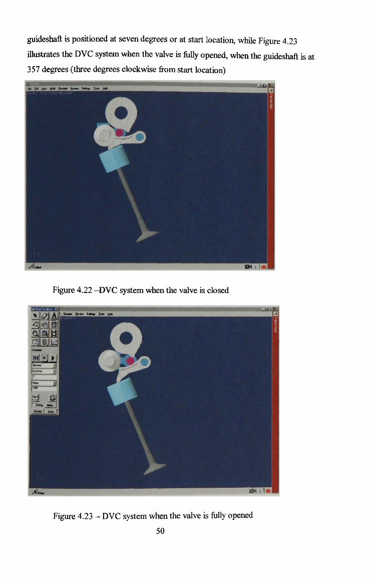
guideshaft is positioned at seven degrees or at start location, while Figure 4.23

illustrates the D V C system when the valve is fully opened, when the guideshaft is at

357 degrees (three degrees clockwise from start location)

Figure 4.22 - D V C system when the valve is closed

Figure 4.23 - D V C system when the valve is fully opened

50

4.3 Simulation Results

Once the D V C model was complete, computer simulations were performed under

various operating conditions. The purpose was to determine the valve lifts, velocities,

acceleration and constraint forces generated in the D V C model. Each simulation was

for 1 second, with 50000 steps. The steps represent the total number of times output

information is provided over the entire simulation.

The engine speeds for the DVC simulation were 60 rpm, 3000 rpm, and 6000 rpm

The valve crank is a substitute for the camshaft and the camshaft rotates at half the

speed of the engine. The camshaft speeds are shown in Table 4.2.

Due to the fact there is rotational motion applied to the valve crank for it to drive the

model, these speeds were converted to degrees/sec using the equation below,

oo = RPM/60* 360 (4.1)

Engine Speed (rpm)

60

3000

6000

Camshaft Speed (rpm)

30

1500

3000 J

Converted A D A M S Speed (deg/sec}

180

9000

18000

Table 4.2 - Converted engine and camshaft speeds

51

4.3.1 D V C Valve Profile

The rotational location of the guideshaft determines the valve lift. The guideshaft,

which is connected to the engine management system via a hydraulic mechanism,

rotates according to the engine speed and load much in the same manner as that

developed by Steinberg et al. (1998). The D V C system would use a hydraulic hub

connected to the guideshaft and the E C U would control the valves that supply oil to

the hydraulic hub. However, the D V C design would be simpler because it wouldn't

rotate like those connected to a continuously spinning camshaft. Using A D A M S , the

guideshaft was rotated to fixed positions in increments of 1 degree between minimum

lift and maximum lift.

As the guideshaft rotates clockwise, the valve lift increases and the valve lift

decreases when the guideshaft rotates anti - clockwise. The guideshaft can rotate from

minimum lift to maximum lift in a span of 10 degrees. The valve lifts of the D V C

system are shown in Figures 4.24, 4.25, 4.26, 4.27, 4.28, 4.29, 4.30, 4.31, 4.32, 4.33

and 4.34.

52

ZJ J<i

25 50 75 100 125 150

Valve Crank Rotation [deg]

.T.T.T.T.T.T.T.T.T.T.T.T.T.TM

Figure 4.24 - Valve profile of D V C system at 357 degrees

53

_1

i

4 a

*)

Al

12.00

10.00

8.00

E

g 3 6.00

5 a

>

4.00

2.00

0.00

/ " \

\

\

/

I \

25 50

-Guide 358d eg

75 100 125 150

Valve Crank Rotation [deg]

175 200 225

Figure 4.25 - Valve profile of D V C system at 358 degrees

54

12.00

10.00

5 00

6.00

4 00

2.00

0.00

/ \

1 1 \

-Guide 359deg

0 25 50 75 100 125 150 175 200 225

Valve Crank Rotation [deg]

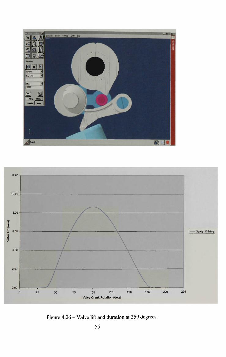
Figure 4.26 - Valve lift and duration at 359 degrees.

55

i PiifTa'm.'v'MgiP—i I A j | JinJete fie»ie« Ssftnoi I o * a«t>

^1 a n

AJ

M S.niaior.

pynmc

"3

r Dttbug Mof... |

Rondo Icon*

JLfUBl

»

12.00

10.00

8.00

3

6.00

4.00

2.00

0.00

25 50

| Guide Odeg )

75 100 125 150

Valve Crank Rotation [deg]

175 200 225

Figure 4.27 - Valve lift and duration at 0 degrees.

56

10.00

8.00

5

6.00 | Guide 1deg [

4.00

2.00

0.00

25 50 75 100 125 150 175 200 225

Valve Crank Rotation [deg]

Figure 4.28 - Valve profile of D V C system at 1 degree

57

12.00

10.00

(00

4.00

2.00

0.00

-Guide 2deg |

0 25 50 75 100 125 150 175 200 225

Valve Crank Rotation [deg]

H

Figure 4.29 - Valve profile of the D V C system at 2 degrees.

58

1

n

IDynam

Sfixiatc Bevww Setimos Iooh Hop - • —

Dynamo

1 [**• 3

r Debug Mae... |

Render I Icon j %

10.00

100

j 6.00

S

1 4.00

0.00

/ \ \

/ \

25 50 75 100 125 150

Valve Crank Rotation [deg]

175 200 225

Figure 4.30 - Valve profile of D V C system at 3 degrees.

59

12.00

10.00

too

5 6.00 -Guide 4deg

4.00

2.00

0.00

25 50 75 100 125 150

Valve Crank Rotation [deg]

175 200 225

Figure 4.31 - Valve profile of D V C system at 4 degrees.

60

12.00 -

?

§ 6.00 -, a

> 5 >

4.00 -

2.00 -

'

25 50

/ \ .

75 100 125

Valve Crank Rotation [deg]

150 175 200 27

—Guide 5deg j

5

Figure 4.32 - Valve profile of D V C system at 5 degrees.

61

12.00

10.00

8.00

6.00

2

4.00

-Guide 6deg |

2.00

0.00^

25 50 75 100 125

Valve Crank Rotation [deg]

150 175 200 225

Figure 4.33 - Valve profile of D V C system at 6 degrees.

62

_, OkfPJi

u_j]

/2

3

Aj a

- ll S>™J-»

AJbm*

il Mil

SirnJKiori

jsnaial |D«fwrnc _*] 1

End im'-i

rr~ [si,,.,

roooo

W| @ll r Debug More |

FkndM | Icora j |

Bt

10.00

8.00

600 -Guide 7deg [

4.00

2.00

0.00

25 50 75 100 125 150

Valve Crank Rotation [deg]

175 200 225

Figure 4.34 - Valve profile of D V C system at 7 degrees.

63

Figures 4.24 to 4.34, show the valve lifts from maximum lift in Figure 4.24 to almost

zero lift in Figure 4.34. The D V C system moves the valve from a maximum lift of

10.70 m m to virtually zero lift in a span of 10 degrees rotation of the guideshaft.

Maximum lift of 10.70 millimetres is achieved when the guideshaft is positioned at

357 degrees (three degrees clockwise from start location), with the valve lift

decreasing at about one millimetre with every 1 degree rotation of the guideshaft. For

example, Figure 4.25 shows the valve lift when the guideshaft is at 358 degrees, with

the lift being 9.73 m m , while Figure 4.26 shows the valve lift at 8.63 m m , when the

guideshaft is positioned at 359 degrees. As the guideshaft begins to rotate anti -

clockwise from the maximum valve lift position of 357 degrees, the valve lift

gradually decreases. The positions of the guideshaft as seen from Figures 4.24 to 4.34,

illustrate the different positions of the guideshaft and their subsequent effect on the

valve lift. Minimum lift is achieved when the guideshaft is at 7 degrees, as seen in

Figure 4.34, the valve lift is 0.36 m m which is virtually zero.

This result confirms that due to the DVC system being able to achieve almost zero

valve lift, there is no need for the throttle, as the valves themselves can limit the

pressures in the cylinders and as a consequence, limit engine output. The most

important aspect that can be seen from the figures, is that the D V C system can

achieve a variation in lift, which means that any valve lift between zero to maximum

lift is quite attainable. Figure 4.35 illustrates the variable lift of the D V C system and

Figure 4.36 illustrates the maximum valve lift versus valve crank rotation. It can be

seen from Figure 4.36 that the relationship between maximum valve lift and valve

crank rotation is fairly linear.

64

Figure 4.35 - Variable lift of D V C system

Maximum Valve Lift versus Valve Crank Rotation

Figure 4.36 - Plot of maximum valve lift versus valve crank rotation

65

The valve timing in conventional engines is fixed at a certain lift, which is basically a

compromise only suited to one engine speed. The Vectra engine, which was utilised

for this project, has its maximum valve lift fixed at 9 m m , as can be seen in Figure 3.4.

The D V C system, as seen in Figures 4.24 to 4.34 also shows that apart from it being

able to achieve a variation in valve lift, its maximum valve lift is also greater than the

Vectra's maximum valve lift. B y having a greater valve lift, greater power can be

generated. It is also quite possible for the D V C system to achieve a greater valve lift

than 10.70 m m . The reason for not pursuing a greater lift than 10.70 m m was because

there is a danger that the valves could hit the pistons at T D C (Top Dead Centre). In

order to increase the lift, modifications to the pistons would need to be made, however

that was beyond the scope of this project. Nevertheless the results show that the D V C

system can achieve a greater maximum valve lift than the Vectra and unlike the

V T E C system developed by Hosaka et al. (1991) and further advanced by Matsuki et

al. (1996) it can achieve continuously variable valve lift between minimum and

maximum lift.

Another notable outcome of the simulation results was that the DVC system's valve

duration can be larger than the Vectra's. The maximum valve duration for the D V C

system when the valve was opened fully at 10.70 m m , was 140 degrees, as can be

seen in Figure 4.24. As the valve lift of the D V C system decreases, the valve duration

is reduced accordingly, as can be seen in Figure 4.35. For instance, at mid-range lift,

when the guideshaft was positioned at 2 degrees, the valve lift was 5.25 m m , while

the corresponding valve duration was 90 degrees. While at minimum lift, 0.36 m m ,

which is when the guideshaft is positioned at 7 degrees, the valve duration is 35

degrees. Due to the system being able to achieve zero valve lift, the valves themselves

can act as a throttle by limiting pressure into the cylinders. As a consequence, air can

flow faster into the cylinder, which improves the mixing of the fuel and air better and

reduces emissions and fuel consumption.

An engine fitted with the DVC system would have a 'drive by wire' "throttle" in

which the accelerator position is input to the Engine Control Unit (ECU) as a voltage.

The E C U would determine h o w much to throttle the engine by taking the accelerator

66

voltage into account. A n engine would be throttled by modulating the amount of inlet

valve lift and duration. For example if the engine is meant to be idling, the guideshaft

would oscillate back and forth in response to the engine speed. If the engine speed

begins to decrease below the idle set point, the guideshaft would rotate a little to

increase the valve lift and duration until the speed increases. W h e n the engine

accelerates, the E C U would respond by rotating the guideshaft sufficiently to respond

to the driver's desired amount of power. While cold starts would be taken care of by

the engine temperature input to the E C U .

From the Figures, it can be seen that valve lift and duration are coupled in the DVC

system. It is proposed that fight loads would be accomplished by reduced valve lift

and contracted duration resulting in a delayed inlet valve opening if the D V C system

is used in isolation. However, the system will employ a phase shifting drive to the

valve crank so that inlet valve opening timing can be optimised. The performance

implications of using valve lift variation for load regulation can be demonstrated by

reference to the performance of B M W ' s Valvetronic series of engines n o w available

in Australia. Valvetronic has almost identical valve motion characteristics to the D V C

system. Edgar (2001) stated that the Valvetronic does not utilise a throttle to control

engine load, much like the D V C system, the valve lift can be reduced so close to zero

lift that the engine is throttled by the inlet valves. By pressing on the throttle pedal

the engine management system increases the amount of inlet valve lift to allow more

airflow and therefore more power. The same can be achieved with the D V C system.

The DVC system will also use a low reduction worm gear drive to control the rotation

of the guideshaft. Wear of critical components such as the guideshaft profile, gudgeon

pin and rocker arm would result in valve lift scatter. The scatter would have most

effect at very low load such as idle. This could be compensated for to a considerable

degree by the engine management system. Also by adherence to conventional

specifications for materials, contact pressures and lubrication, the D V C system would

have similar wear characteristics as conventional valve trains.

67

Figure 4.37 illustrates a comparison between the valve profile of the D V C system and

the existing Vectra engine.

Figure 4.37 - Comparison of valve lifts between the D V C system and the Vectra

cylinder head.

It can be seen from Figure 4.37 that not only does the DVC system have a greater

maximum lift than the Vectra, but also, its valves are able to stay open for a longer

period than the Vectra's valves. This increased valve duration produces greater power

at higher rpm.

68

4.3.2 Valve Velocity and Acceleration Results

As the speed of the DVC system is increased, the acceleration and velocity of the

valve also increases. The position of the guideshaft, also affects the acceleration and

velocity of the valve. With greater valve lift, the velocity and acceleration increase,

but decreasing valve lift, decreases the velocity and acceleration. The valve velocity

and acceleration plots are shown in Figures 4.38,4.39, 4.40, 4.41,4.42,4.43,4.44,

4.45 and 4.46. The peak accelerations and velocities versus valve crank rotation are

shown in Figures 4.47 and 4.48 respectively.

69

I

2.5E-t07

2.0E+07

1.5E+07

g 1.0E+07

e

8 it

5.0E+06

O.OE+OO

100

Rotation [deg]

(a)

200

4! 1000 E

U

a

Rotation [dog]

0>)

Figure 4.38 - Plot of (a) velocity and (b) acceleration at 18000 degrees/sec

with guideshaft positioned at 357 degrees.

70

4.00E+03

3.00E+Q3

2.00E+03

•3 1.00E+03

§ O.OOE+00

-1.00E+03

-2.00E+03

-3.00E+03 -

Rotation [cleg]

(a)

1.60E+07

1.00E+07

j? 8.00E+06

| 6.00E+06

E a 8 ^ 4.00E+06

O.OOE+00

-2.00E+06

— • - — - — . — — . . — _ .

\— - r -

\ ll

I \ J \ v_

\

y v - " ' '

100 120

Rotation [deg]

(b)

Figure 4.39 - Plot of (a) velocity and (b) acceleration at 18000 deg/sec with guideshaft positioned at 2 degrees.

71

5.00E+02 I

4.00E+02

3.00E+02

2.00E+02

1.00E+02

>. O.OOE+00

-1.00E+02

-3.00E+02

-4.00E+02

-5.00E+02

50 150 250

Rotation [deg]

(a)

2.50E+06

K- 1.50E+06

<

I E, g" 1.00E+06

e a 9 | 5.00E+05

O.OOE+00 -

-S.00E+O5

-1.50E+06

40

^ 80 100 120

Rotation [deg]

140 160 200

(b)

Figure 4.40 - Plot of (a) velocity and (b) acceleration at 18000 deg/sec,

with guideshaft position at 7 degrees.

72

2.50E+03

2.00E+03

-1.50E+03

-2.00E+03I

7.0OE+06

3.00E+06

O.OOE+00

-1.00E+06

Rotation [deg]

(a)

^ r _ _ ^ 100 150

Rotation [deg]

(b) Figure 4.41 - Plot of (a) velocity and (b) acceleration at 9000 degrees/sec, with guideshaft position at 357 degrees.

73

2.00E+03 |

1.50E+03

1.00E+03

« 5.00E+02

•f O.OOE+OO

-5.00E+02

-1.00E+03

-1.50E+03 .

50 100 150

Rotation [deg]

(a)

200

n 2.50E+06

£ 1.00E+06

SO 100 150

Rotation [deg]

200

(b) Figure 4.42 - Plot of (a) velocity and (a) acceleration at 9000 degrees/sec, with guideshaft positioned at 2 degrees.

74

2.50E+02

2.00E+02

1.50E+O2

1.00E+02

5.00E+01

I E >. O.OOE+OO

f o

1 -5.00E+01 -1.00E+02

-1.50E+02

-2.00E+02

50 150 200

-2.50E+02

Rotation [deg]

(a)

3.50E+06 -i—

2.50E+06

ST

<

I £ = 1.50E+06 | v

e a

5.00E+05

-5.00E+05 f 100 1 5 0

Rotation [deg]

200

(b) Figure 4.43 - Plot of (a) velocity and (b) acceleration at 9000 degrees/sec, with guideshaft positioned at 7 degrees.

75

5.00E+01

4.00E+01

3.00E+01

2.00E+01

| 1.00E+01

E,

£• o 1 O.OOE+OO

-1.00E+01

-2.00E+01

-4.00E+011

5.00E+01 1.00E+02 1.50E+02

Rotation [deg]

(a)

2.00E+02

5.00E+02

O.OOE+00

-S.00E+02 100 150

Rotation [deg]

(b) Figure 4.44 - Plot of (a) velocity and (b) acceleration at 180 degrees/sec, with guideshaft positioned at 357 degrees.

76

4.00E+01

3.00E+01

2.00E+01

4 1.00E+01

E

5 O.OOE+00

0.(

-1.00E+01

-2.00E+01

OOE+00 2.00E+01 4.00E+01 6.00E+01 8.00E+01 1.00E+02 1.20E+02 1.40E+02 1.60E+02 1 80E+02 2.00E+' 02

-3.00E+01 -

2.50E+03

2.00E+03

1.50E+03

Rotation [deg]

(a)

ET

o 1.00E+03

5.00E+02

0.0OE+O0

-5.00E+02

20 40

(b) Figure 4.45 - Plot of (a) velocity and (b) acceleration at 180 degrees/sec, with guideshaft positioned at 2 degrees.

77

5.00E+00

4.00E+00

3.00E+00

2.00E+OO

1.00E+00

g. O.OOE+OO

g 0.00£+(

-1.00E+00

-2.00E+00

-3.00E+00

-4.00E+00

-5.00E+00I

5.00E+01 1 00E+02 1.50E+02 2.00E+02 2.50E+02

Rotation [deg]

(a)

2.00E+03

1.50E+03

5.00E+02

O.ME+00

-5.00E+02

50 100 150

Rotation [deg]

200 250

(b) Figure 4.46 - Plot of (a) velocity and (b) acceleration at 180 degrees/sec, with guideshaft positioned at 7 degrees.

78

Peak Accelerations versus Valve Crank Position

180 [cleg/sec]

- 9000 [deg/sec]

18000 [deg/sec]

-Linear (18000 [deg/sec])

-Linear (9000 [deg/sec))

•Linear (180 [deg/sec])

90

Figure 4.47 - Plot of peak acceleration versus valve crank rotation

Peak Velocities versus Valve Crank Rotation

-i J

Valve Crank Rotation [deg]

Figure 4.48 - Plot of peak velocity versus valve crank rotation

79

It can be seen from Figures 4.38 to 4.46, that both the valve velocity and acceleration

result was greatly influenced by the speed of the system and its valve lift position. At

minimum lift, irrespective of the D V C operating speeds of 180 degrees/sec, 9000

degrees/sec and 18000 degrees/sec, the valve velocity and acceleration are practically

zero. This is due to the fact that at minimum lift, the valve is virtually closed.

As the DVC speed was increased from 9000 degrees/sec, to 18000 degrees/sec, the

valve velocity and acceleration also increases. It can be seen in Figure 4.38, that the

maximum acceleration and velocity of the valve, when the D V C system was

operating at 18000 degrees/sec was 2.35e7 mm/sec2 and 4.33e3 mm/sec respectively.

As the valve lift decreases, the velocity and acceleration also decrease, as seen in

Figure 4.39 and 4.40. It can be seen that the maximum acceleration and velocity was

1.42e7 mm/sec2 and 2.90e3 mm/sec respectively, when the guideshaft was positioned

at 2 degrees. While at 7 degrees (minimum lift), the acceleration and velocity was

practically zero. At mid-range lift (guideshaft positioned at 2 degrees) the valve

velocity and acceleration speed was half the velocity and acceleration speed when at

maximum lift (guideshaft positioned at 357 degrees).

Figures 4.47 and 4.48 illustrate that the relationship between the peak accelerations

and velocities versus the valve crank rotation are essentially linear.

The valve velocity and acceleration results illustrate that when the DVC system was

operating at higher speeds and at a greater valve lift, a higher acceleration and

velocity was needed to open the valve off its seat and consequently a greater force

was required to open the valve.

80

4.5 Force and Stress Analysis of Components

The DVC system modeled using ADAMS software demonstrated the feasibility of the

system and its valve timing sequencing. However the component forces generated at

operational speeds need to be evaluated, hence the stress analysis of the most

important D V C component, the rocker arm, can be carried out to assess whether it can

withstand the forces acting on it.

The kinematic and dynamic predictions from the ADAMS simulation of the DVC

system allowed the assessment of the loads on the system components. With the D V C

system operating at its highest speed of 18000 deg/sec, or 6000 rpm, the "worst case"

loads on the rocker arm (which is the part under the greatest bending load) were

estimated.

The two most significant aspects of the DVC component loading investigated are the

Herztian contact pressures between the gudgeon pin and the guideshaft and localised

stresses on the rocker arm due to bending. The line contact force between the gudgeon

pin and guideshaft must not exceed a level that would create excessive Hertzian

contact pressures. The second aspect was to ensure that the repetitive loading of the

rocker arm does not create localised stresses that exceeded the fatigue limit of the

proposed materials.

The hand calculation of the Hertzian contact pressures was based on the line contact

between the gudgeon pin and guideshaft obtained from the A D A M S simulation. The

loads acting on the rocker arm were obtained and then processed using a finite

element package, called Cosmos/DesignStar. The stress estimations determined

whether the rocker arm could withstand the stress placed on it.

The contact forces obtained from ADAMS and the stress estimations from

Cosmos/DesignStar were evaluated.

81

4.5.1 Forces Acting on D V C Components

The maximum contact forces between the moving parts of the DVC system were

obtained from A D A M S simulation. The contact force results can be seen in Figures

4.49,4.50,4.51, 4.52, 4.53, 4.54, 4.55, 4.56, 4.57, 4.58, 4.59 and 4.60. The peak

forces versus valve crank rotation results can be seen in Figures 4.61, 4.62, 4.63 and

4.64.

When the valve is closed, the force acting between the components, which is the point

where the valve is to be pushed down, is only the spring force, hence the reason why

in the Figures, the contact force begins at 300 N. The spring rate was based on the

measured spring rate from the standard Vectra engine cylinder head. The reason that

the plot does not begin at zero is because the D V C system as modeled using A D A M S

does not include a valve seat. In an automotive engine the valve seat would absorb

that force, and as a result for our purposes the strength of the spring was not

important. The reason the D V C system does not include a valve seat is because the

model would be too complicated for A D A M S to compute. As a result the valve train

of the D V C system as modeled using A D A M S was pre-stressed.

82

Figure 4.49 - Rocker A r m to Bucket Force at 18000 degrees/sec

Figure 4.50 - Gudgeon Pin to Guideshaft Force at 18000 degrees/sec

83

Figure 4.51 - Gudgeon Pin to Rocker A r m Force at 18000 degrees/sec

3.00E+03

2.50E+03

2.00E+03

1.50E+03

1.00E+03

5.00E+02

O.OOE+00

50 100 150

Rotation [deg]

357 deg

2 deg

-7 deg

250

Figure 4.52 - Rockershaft Force at 18000 degrees/sec

84

1000 -i

900

800

700

600

g 500

400

300

200

100-

"

357 deg

2deg

7 deg

CT

50 100 150

Rotation [deg]

200 250

Figure 4.53 - Rocker A r m to Bucket Force at 9000 degrees/sec

3.00E+03 1

2.50E+03

2.00E+03

1 50E+03

1.00E+03

5.00E+02

0.00E+O0

357 deg

2deg

7 deg

0.00E+00 5.00E+01 1.00E+02 1.50E+02 2.00E+02 2.50E+02 3.00E+02

Rotation [deg]

Figure 4.54 - Gudgeon Pin to Guideshaft Force at 9000 degrees/sec

85

2.50E+03

2.00E+03

1.50E+03

1.00E+03

5.00E+02

O.OOE+00

LJL1 LJJMJilJyillJI s

^Jt

J

/ \

/

1 \ \

yy ^ lv [ \, 1

357 deg

-2 deg

7 deg

O.OOE+00 5.00E+01 1.00E+02 1.50E+02 2.00E+02 2.50E+02 3.00E+02

Rotation [deg]

Figure 4.55 - Gudgeon Pin to Rocker Arm Force at 9000 degrees/sec

1.60E+03

1.40E+03

1.20E+03

LODE+03

I S 8.00E+02

£

6.00E+02

4.00E+02

2.00E+02

0.00E+00

50 100 150

Rotation [deg]

200 250

Figure 4.56 - Rockershaft Force at 9000 degrees/sec

86

357 deg

"2 deg

7 deg

100 150

Rotation [deg]

Figure 4.57 - Rocker A r m to Bucket Force at 180 degrees/sec

+ 03

g 8 1.50E + 03

3 57 deg

-2 deg

7 deg

Figure 4.58 - Gudgeon Pin to Guideshaft Force at 180 degrees/sec

87

2.50E+O3

2 00E+O3

1.50E+O3

1.00E+03--

5.00E+O2 S

O.OOE+OO 5.00E+01 1.00E+O2 1.50E+O2

Rotation [deg]

2.00E+02 2.50E+02

Figure 4.59 - Gudgeon Pin to Rocker A r m Force at 180 degrees/sec

1.80E+03 i

1.60E+03

1.40E+03

1.20E+03

^ 1.00E+03

"• 8.00E+02

6 00E+02

4.00E+02

2.00E+02

0.00E+00

20 40 60 80 100 120

Rotation [deg]

Figure 4.60 - Rockershaft Force at 180 degrees/sec

88

357 deg

2 deg

7 deg

140 160 180 200

Peak Bucket to Rocker Tip Forces versus Valve Crank Rotation

3000

180deg/s

9000 deg/s

18000 deg/s

Linear (18000 deg/s)

Linear (9000 deg/s)

Linear (180 deg/s)

Figure 4.61 - Plot of peak bucket to rocker arm forces versus valve crank rotation

Figure 4.62 - Plot of peak gudgeon pin to guideshaft forces versus valve crank

rotation

89

Peak Pin to Rocker Forces versus Valve Crank Rotation

6000 -|

40 60 80

Valve Crank Rotation [deg]

Figure 4.63 - Plot of peak gudgeon pin to rocker arm forces versus valve crank rotation

Peak Shaft to Rocker Forces versus Valve Crank Rotation

180 deg/s

-9000 deg/s

18000 deg/s

-Linear (18000 deg/s)

-Linear (180 deg/s)

40 60 80

Valve Crank Rotation [deg]

y = -95.851x+10473

120

Figure 4.64 - Plot of peak rockershaft forces versus valve crank rotation

90

At maximum speed of 18000 degrees/sec and maximum lift, a maximum gudgeon

pin/rocker arm contact force of 5000N was obtained. This force is necessary for

determining the bending load on the rocker arm. It has not been considered for

Hertzian contact pressure calculation because it will not be a line contact in a future

prototype. The force acting on the rockershaft was 2500N and that between the rocker

arm and bucket was also 2500N. This can be seen from Figures 4.51, 4.52 and 4.49

respectively. The contact force between the gudgeon pin and guideshaft was higher

than the opposing gudgeon pin/rocker arm force. From Figure 4.50, it can be seen that

the gudgeon pin/guideshaft force was 7300N. The reason for the higher force is due to

the fact that the gudgeon pin is pushing the guideshaft on an angle with respect to the

gudgeon pin to rocker arm. It is this non-aligned component that raises the net force.

As the initial thrust of acceleration is over, the force drops and remains low while the

valve is near constant velocity as it begins to get closer to its fully opened position.

When the valve reaches its fully opened position, an opening force of 650N was

obtained between the rocker arm/bucket, 2000 N between gudgeon pin/guideshaft,

1800 N between gudgeon pin/rocker arm and 1200 N for the rockershaft. Fully open,

the valve stops and then changes direction, therefore the force is not constant, due to

the fact there is some friction to be overcome. As the valve begins to close, the

friction reduces the load on the gudgeon pin and it is harder for the spring to push

back when the valve closes. This is because friction actually is helping to slow the

valve by opposing motion, and the reason, as seen in all the figures, the valve closing

peaks are much lower than the valve opening peaks.

With decreasing rotational speed and valve lift, the forces acting between the

components also decreased accordingly. Figures 4.53 to 4.60, show the forces at 9000

degrees/sec and at 180 degrees/sec and it can be seen that as the valve lift and speed

decreases, it has a noticeable effect on the forces. The maximum peak forces are

considerably lower than when the valve is operating at 18000 degrees/sec for all valve

lifts. For example, if w e compare the contact forces between the rocker arm and

bucket at 18000 degrees/sec, 9000 degrees/sec and at 180 degrees/sec, it can be seen

91

that the contact forces are much lower at decreasing speeds. The contact force

between the rocker arm and bucket at 18000 degrees/sec, as mentioned previously

was 2500 N. From Figure 4.53, it can be seen that at 9000 degrees/sec, the contact

force between the rocker arm and bucket is 920 N. At the maximum speed of 18000

degrees/sec, the contact force obtained between the gudgeon pin and guideshaft was

7300 N , while at 9000 degrees/sec, the contact force decreased to 2700 N. The contact

force between the gudgeon pin and rocker arm at 9000 degrees/sec was 1600 N, while

at 18000 degrees/sec it was 5000 N. The force acting on the rockershaft at 9000

degrees/sec was 800 N , as compared to 2500 N at 18000 degrees/sec.

At 180 degrees/sec, it can be seen from the figures that for all the components, the

only contact force acting is the spring force of 300 N, as the system is virtually

operating at idle, and inertia is nearly zero.

The guideshaft position also affects the contact forces. The lower the valve lift the

less the contact force between the components. For example the contact force

obtained between the rocker arm and bucket, when the guideshaft is at maximum lift

(357 degrees), was 2500 N , as shown in Figure 4.49. While when the guideshaft was

at mid-range lift (2 degrees), the contact force was 1600 N. The contact force obtained

between the gudgeon pin and guideshaft at maximum lift, was 7300 N, while at mid-

range lift, the force decreased to 4800 N , as shown in Figure 4.50. While the contact

forces acting between the gudgeon pin and rocker arm and on the rockershaft also

decreased between maximum lift and mid-range lift.

At 9000 degrees/sec, again the contact forces are lower at lower valve lifts, than at

maximum valve lift. Figure 4.53 shows the contact force between the rocker arm and

bucket, and it can be seen that the contact force at maximum lift, was 920 N, while at

mid-range lift, it was 660 N. The contact force between the gudgeon pin and

guideshaft at maximum lift was 2600 N, while at mid-range lift, it was 1700 N, as

seen in Figure 4.54. The contact force between the gudgeon pin and rocker arm at

maximum lift was 1750 N , while at mid-range lift it was 1450 N. While the contact

force acting on the rockershaft at maximum lift was 800 N and at mid-range lift 780

N. 92

At minimum lift (7 degrees anti-clockwise guideshaft adjustment), it can be seen from

all the figures, that at 18000 degrees/sec and at 9000 degrees/sec, the only force acting

was the spring force because the valve lift is virtually zero. While at 180 degrees/sec

as seen from Figures 4.57 to 4.60, whether at maximum lift or at rninimum lift, the

only force acting was the spring force because interia was low.

The results show that the forces vary with valve lifts and speeds, a higher valve lift

and speed produces higher forces. The reason that the forces are lower at decreasing

speeds and valve lifts, is due to the fact that once the valve begins to move off its seat

the change in momentum is not as great, as it is at higher speeds and higher valve

lifts.

The highest contact force peaks between all the components occur as the valve is

beginning to open. This is due to the fact that as the valve begins to be pushed open, it

must accelerate off the valve seat and in addition during opening the friction resists

the acceleration.

From the peak force figures it can be seen that the forces acting between the

components are linear except for the peak force of the rockershaft when the system is

operating at 9000 degrees/sec. Also the peak gudgeon pin to the rocker arm force

when the system is also operating at 9000 degrees/sec is not linear. This can be seen

from Figures 4.64 and 4.63 respectively. The non-linearity is due to the fact that the

peaks occur at different phases of motion. This is probably due to friction on the valve

and also the way in which the gudgeon pin moves along the guideshaft and rocker

arm.

4.5.2 Stress Analysis

The stress analysis of the rocker arm was conducted using Cosmos/DesignStar.

Cosmos/DesignStar is a F E A package that allows stress analysis on components

created in any of the major C A D packages.

93

The rocker arm, as previously stated was created in SolidWorks, and subsequently it

was imported into Cosmos/DesignStar in a first attempt to evaluate whether it could

withstand the loads acting on it. The rocker arm as imported into Cosmos/DesignStar

is shown in Figure 4.65.

£* V»w e«r« 1«* EMS «*>• W " * * tl*

eg a #tm? ^ ^ C K O * « B B I B O «v «> 'q'iq^i* / ,•& 1 % J\ iL Z* ® & g ^ * JJA f |l«n«nc zl

-l»l*l

% .-4 *tj A) Ij if 4i --fe

4 • • W * * J.

Figure 4.65 - F E A of rocker arm in Cosmos/DesignStar

Once the rocker arm was imported into Cosmos/DesignStar, the type of analysis

performed needed to be selected and the material of the component defined. Static

analysis was selected and the material for the rocker arm selected was A S T M 40-41

alloy steel.

Once the material and type of analysis were selected, the rocker arm had to be

constrained. A load of 5000 N acting on the top of the rocker arm was defined, with a

fixed constraint acting on the pivot, and a prescribed constraint which allowed

94

translation in the x direction only, acting at the tip of the rocker. Once the constraints

on the rocker arm were defined, the component was meshed, and the analysis of the

rocker arm was completed. The F E A results of the rocker arm can be seen in Figures

4.66 to 4.67.

Ivan-static:: Static Nodal Stress

Units: IM/rn'S Deformation Scale 1 : 557864

Von Mises

1 1 000e+009

9.168e+008

8.335e+008

7.502e+Ci03

S.670e+008

5.838e+008

•5.005e+008

4.172e+008

!3.340e+008

2.5088+008

1,675e+008

B.425e+007

h 000e+00 6

Figure 4.66 - F E A Analysis of rocker arm

95

Ivan-static:: Static Nodal Stress

Units: NAnA2 Deformation Scale 1 : 5.87864

Figure 4.67 - F E A Analysis of rocker arm

The maximum fatigue limit of fully reversed alloy steel is 500 Mpa. As can be seen

from Figures 4.66 and 4.67, the rocker arm exhibits excessive stress, especially in the

centre on the non-contact side, as seen in Figure 4.67.

Component design and FEA analysis is an iterative process and in order to reduce this

stress, gradual changes such as strengthening the non-contact side of the rocker arm,

by thickening the rocker vertical and adding a flange to the non-contact side, were

tried and the resulting stress patterns, as seen in Figure 4.68 to 4.69 are shown.

96

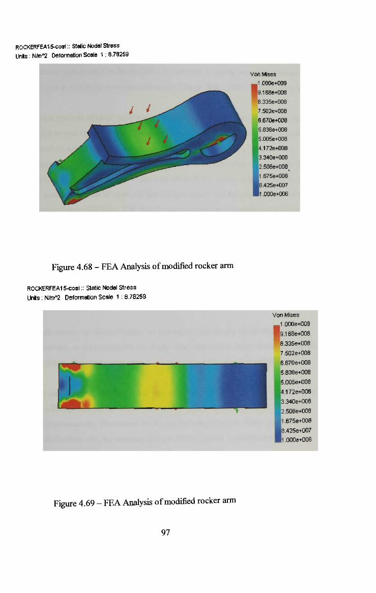
ROCKERFEA15-cosi:: Static Nodal Stress

Units: NAn^ Deformation Scale 1: 8.78259

Von Mses

1 000e+009

.1686+008

8.335e+008

7.502e+008

6.670e+008

5.838e+00S

5.005e+008

4.172e+008

3.3406+008

2.508e+008)

1,675e+008

|8.4256+007

1.0006+006

Figure 4.68 - F E A Analysis of modified rocker arm

ROCKERFEA15-cosi:: Static Nodal Stress

Units: NAnA2 Deformation Scale 1 : 8.78259

Von Mises

1 1 000e+009

9.168e+008

8.335e+008

7.502e+008

6.6706+008

5.838e+008

5.0056+008

n4.172e+008

3.340e+008

|2.508e+008

H ,675e+008

8.425e+007

ll 000e+006

Figure 4.69 - F E A Analysis of modified rocker arm

97

As can be seen from Figures 4.68 and 4.69, the stress concentrations of the rocker arm

are reduced significantly in the modified rocker a r m It can be seen that most of the

component is within the maximum allowable fatigue limit of 500 M p a for alloy steel.

Statistical analysis of alloy steels (case hardened) has shown that their fatigue strength

is limited to plus or minus 500 M p a in the case of fully reversed stress such as that

produced by a rotating beam in bending. However if the stress is limited to an

oscillating load in one direction of either tension or compression only, then the fatigue

strength increases to 800 Mpa. In the case of the D V C rocker arm, it could be argued

that a significant factor of safety against fatigue failure would arise if the maximum

stress were below 500 Mpa. This would guard against any possibility of fully reversed

stress. However, due to the limited space available for the rocker arm in the standard

Vectra cylinder head, the stress due to bending across the restricted centre section

remained above 500 M p a through several design iterations, as seen in Figure 4.69.

Given the nature of the rocker arm's operation, it is unlikely that the stress will be

reversed. Therefore, it is likely that the rocker arm will not suffer a fatigue failure

because the maximum stress is below 800 Mpa.

The high stresses at the constraints are unrealistic and should not be taken into

consideration, as the constraints are single dimension points, hence the reason for the

high stresses. They were only used to allow the model to function appropriately.

It must also be noted that the rocker arm as modeled using ADAMS and analysed in

Cosmos/DesignStar has no fillets, only square edges, which is not ideal for actual

stress concentrations. The reason for the rocker arm having no fillets was that it

avoids difficulties with the meshing process. However the actual production

component would have fillets and the rocker arm would be stronger.

98

4.5.3 Hertz Contact Pressure

The preferred standard production cylinder head material is nodular iron, for high

stress surfaces such as camshafts. According to Gaffriey and Redington (1998),

nodular iron can withstand contact pressures of up to 1700 MPa.

The maximum Herztian contact pressure obtained between the gudgeon pin and

guideshaft was 996 M P a (refer to Appendix C). However, the guideshaft and gudgeon

pin will be made from A S T M 40-41 alloy steel, which is a stronger material than

nodular iron. The alloy steel would be case hardened, which would give it a

satisfactory contact resistance.

99

5 CONCLUSIONS AND RECOMMENDATIONS

5.1 Conclusions

A cylinder head test rig was constructed to measure the valve lift profile of the

standard Vectra engine cylinder head. The D V C system was successfully simulated

using A D A M S software for its valve lift profile and loads acting on the components.

The stress analysis of the key component of the D V C system, the rocker arm was

carried out.

The following conclusions can be drawn from the research reported here:

• The valve lift profile of a standard Vectra engine was determined using the

test rig constructed for that purpose.

• Simulation of the proposed DVC system demonstrated that the system has

variable lift characteristics which can achieve any valve lift between

maximum and minimum, according to engine speed.

• According to the results of the DVC simulation, a maximum valve lift of

10.70 m m was attained compared to a maximum of 9 m m for the standard

Vectra engine.

• The minimum lift obtained during simulation of the DVC system was

practically zero, therefore it seems reasonable to infer that a throttle would not

be required with the proposed system.

100

• Analysis of the rocker arm indicated that the loads imposed on it would not

lead to failure under repeated bending loads, while the Hertzian contact

pressure between the gudgeon pin and the guideshaft was within the maximum

allowable contact pressure.

5.2 Recommendations for Future Work

The following recommendations are proposed for future research:

• A DVC system should be designed, constructed and fitted to the existing

Vectra engine.

• Performance tests on the Vectra engine with the DVC system including fuel

consumption and emission tests, should be carried out and compared with

results obtained from the standard Vectra engine.

101

6 REFERENCES

Ashley, C , (1995), Powertrain Development, Automotive Engineer, Vol. 20, pp. 20

Bassett, M.D., Blakey, S.C. and Foss, P.W., (1997), A Simple Two-State Late Intake

Valve Closing Mechanism Proe. I. Mech. Vol. 211.

Brauer, K, (1999), Valve Timing is Everything, www.edmunds.com

Crohn, M. and Wolf, K., (1990), Variable Valve Timing in the New Mercedes-Benz

Four-Valve Engines, SAE 891990

Deeg, E.W., (1992), New Algorithms for Calculating Hertzian Stresses,

Deformations, and Contact Zone Parameters, AMP Journal of Technology, Vol.2,

pp.14-22

Desantes, J., Payri, F. and Corberan,J., (1988), A Study of the Performance of a SI

Engine Incorporating a Hydraulically controlled Variable Valve Timing System, SAE

880604

Douglas, E., (1997), EVA Meet Demands for Performance and Economy, Southwest

Research Institute

Edgar, J, (2001), BMW Valvetronic, www.autospeed.com

102

Gaffhey, J. and Redington, P., (1998), Things to Know about Cam Grinding,

Automotive Design and Production, www.autofieldguide.com

Griffiths, P. and Mistry, K.N., (1988), Variable Valve Timing for Fuel Economy

Improvement - The Mitchell System, SAE 880392

Hannibal, W. and Bertsch, A., (1998), VAST: A N e w Variable Valve Timing System

for Vehicle Engines, SAE 980769

Hara, S. and Kumagai, K., (1989), Application of a Valve Lift and Timing Control

System to an Automotive Engine, SAE 890581

Hara, S., Nakajima, Y. and Nagumo, S., (1985), Effects of Intake-Valve Closing

Timing on Spark-Ignition Engine Combustion, SAE 850074

Hatano, K., Iida, K., Higashi., H. and Murata, S., (1993), Development of a New

Multi-Mode Variable Valve Timing Engine, SAE 930878

Herrin, R. and Pozniak, D., (1984), A Lost-Motion, Variable Valve Timing System

for Automotive Piston Engines, SAE 840335

Heywood, J., (1988), Engine Fundamentals, McGraw-Hill

Hosaka, T. and Hamazaki, M., (1991) Development of the Variable Valve Timing an

Lift (VTEC) Engine for the Honda NSX, SAE 910008

103

Hu, H., (1996), Four-Cycle Internal Combustion Engine with Two-Cycle

Compression Release Braking SAE 961123

Kreuter, P., Heuser, P. and Reinicke, J., (1998), The Meta VVH System - A

Continuously Variable Valve Timing System, SAE 980765

Lee, J., Lee, C. and Nitklewicz, J., (1995), The Application of a Lost Motion WT

System to a D O H C SI Engine, SAE 950816

Leone, T.G., Christenson, E.J. and Stein, R.A., (1996), Comparison of Variable

Camshaft Timing Strategies at Part Load, SAE 960584

Lenz, H.P. and Wichart, K., (1988), Variable Valve Timing - A Possibility to Control

Engine Load without Throttle, SAE 880388

Ma, T.H., (1988), The Effect of Variable Engine Valve Timing SAE 880390

Maekawa, K. and Ohsawa, N., (1989,), Development of a Valve Timing Control

System, SAE 890680

Matsuki, M., Nakano, K., Amemiya, T., Tanabe, Y., Shimizu, D. and Ohmura, I.,

(1996), Development of a Lean Burn Engine with a Variable Valve Timing

Mechanism, SAE 960583

104

Moriya, Y , Watanabe, Uda, H., Kawamura, H. and Yosioka, M., (1996), A Newly

Developed Intelligent Variable Valve Timing System - Continuously Controlled Cam

Phasing as Applied to a N e w 3 Litre Inline 6 Engine, SAE 960579

Nakayame, Y, Maruya, T., Oikawa, T. and Fujiwara M. (1994), Reduction of HC

Emission from V T E C Engine During Cold-Start Condition, SAE 940481

Ohyama, Y. and Fujieda, M., (1995), A N e w Engine Control System Using Direct

Fuel Injection and Variable Valve Timing SAE 950973

Payri, F., Boada, F. and Macian V., (1994), Reduction of Pumping Losses by the use

of a Variable Valve System, Proe. I. Mech Vol. 198,

Saunders, RJ. and Abdul-Wahab, E.A., (1989), Variable Valve Closure Timing for

Load Control and the Otto Atkinson Cycle Engine, SAE 890677

Schechter, M. and Llevin M. (1996), Camless Engine, SAE 960581

Shigley, J., (1989), Mechanical Engineering Design, McGraw-Hill Kogakusha

Steinberg, R., Lenz, I. and Koehnlein, G., (1998), A Fully Continuous Variable Cam

Timing Concept for Intake and Exhaust Phasing, SAE 980767

105

Titolo, T., (1991), The Variable Valve Timing System - Application on a V8 Engine,

SAE 910009

Turtle, J., (1982), Controlling Engine Load by Means of Early Intake-Valve Closing

SAE 820408

Urata, Y., Umiyama, H , Shimizu, K., Fujiyoshi, Y. and Fukuo, K., (1993), A Study

of Vehicle Equipped with Non-Throttling S.I Engine with Early Intake Valve Closing

Mechanism, SAE 930820

U.S Department of Energy, (2001), Conserve Resources for Future Generations, Why

is Fuel Economy Important, www.fueleconomy.com

U.S Department of Energy, (1998), Climate Change, Why is Fuel Economy Important,

www.fiieleconomy.com

Vogel, O., Roussopoulos, K., Guzzella, L. and Czekaj, J., (1996) An Initial Study of

Variable Valve Timing Implemented with a Secondary Valve in the Intake Runner,

SAE 960590

Wilson, N., Dobson, C. and Mudell, G., (1993), Active Valve Train, Automotive

Engineer, Vol.18, pp. 42-46

Yagi, S., Miura, S., Satoh, I., Ishibashi, Y. and Nishi, K., (1992) A N e w Variable

Valve Engine applying Shuttle Cam Mechanism SAE 920451

106

Appendix A - Component Measurements

The dimensions of the DVC components (millimetres) are shown from Appendix Al to A8.

Appendix Al - Bucket dimensions

Appendix A2 - Valve Crank dimensions

107

Appendix A3 - Guideshaft dimensions

Appendix A 4 -Rocker Arm dimensions

108

93

010

Appendix A5 - Rockershaft dimensions

0 32)

> )

J

(irc? )

//

Appendfx A 6 - Valve dimensions

109

it) -f r

(R9.50 ) —

S8.50 ]

f " (18)

o Appendix A7 - Conrod dimensions

Ar-^

'^tsy.

(85)

-(010 )

- {0 6)

Appendix A8 - Gudgeon Pin dimensions

110

Appendix B - Constraint Descriptions

The descriptions of the constraints that were used in A D A M S to constrain the D V C

components is shown in Table Bl.

Constraints

Translational Joint

Description

A translational joint allows o n e part to translate along a vector with respect to another part. T h e parts can only translate, not rotate, with respect to each other.

Revolute Joint

Location First pari

Axis of rotation

Second part

A revolute joint allows the rotation of one part with respect to another about a c o m m o n axis. T h e revolute joint can be located anywhere along the axis about which the joint's parts can rotate with respect to each other.

Fixed Joint

Second pari

A fixed joint locks t w o parts together so they cannot m o v e with respect to each

other.

Table Bl - Description of constraints

111

Appendix C - Hertzian Stress Calculations

The Herztian stress calculations between the Guideshaft and Gudgeon Pin is shown in

Table Cl

Calculation of Hertzian Contact Pressure p „ „ of Pin to Guide Based on Adams Simulation of Maximum Contact Force

Includes estimate of required Hardness [HB] for Endurance Strength, Sc, for reliability 0.99 to 0.999% and life >10* cycles

Calculation of contact patch half width

1 - 0.3*2

(1-0.3A2)/E,

1/d,

1/d2

1/d, + 1/d2

[(1-0.3*2)/E,]+[(1-0.3A2)/EJ / [(l/d^-KI/dj)]

2F{[(1-0.3*2)/El]+[(1-0.3*2)/E2] / [(l/dO+OI/dj)]} / Pi L

SQRT(2F{[(1-0.3"2VE,]+[(1-0.3"2)/E2] / [(l/dO+CI/dj)]} / Pi L)

2F/PibL

0.3pm

Calculation of contact pressure

Calculation of fully reversed Shear Stress

Calculation of required surface hardness

(Sc + 70)/2.76

0.91

4.39614E-12

100

-79.36507937

20.63492063

4.26087E-13

1.80015E-07

0.000424282

996]

299

386

Poison's Ratio equals 0.3

Elastic Modulus equals 207 [Gpa]

Pin Diameter equals 0.01 [m]

Guide Diameter equals -0.0126 [m]

Force, F equals 7300 [N] & Guide Width, L equals 0.011 [m]

Contact Half Width, b [ml

Maximum Contact Pressure, p™, [MPa]

Maximum sub surface reversed Snear Stress, T^, [Mpa]

Required Hardness [HB] (Brinell Hardness number)

Table Cl - Calculation of the Hertzian stress between the gudgeon pin and guideshaft

112