Levy Institute Measure of Economic Well-Being Levy Economics Institute of Bard College 3 Preface...

The Levy Economics Institute of Bard College

May 2004

Levy Institute Measureof Economic Well-Being

United States, 1989, 1995, 2000, and 2001

edward n. wolff, ajit zacharias, and asena caner

Levy Institute Measureof Economic Well-Being

This report is available on the Levy Institute website at www.levy.org.

edward n. wolff is a senior scholar at The Levy Economics Institute and a professor of economics at New York University. ajit zacharias

and asena caner are research scholars at The Levy Economics Institute.

Copyright © 2004 The Levy Economics Institute

United States, 1989, 1995, 2000, and 2001


The Levy Economics Institute of Bard College, founded in 1986, is an autonomous research organization. It is nonpartisan, open to the

examination of diverse points of view, and dedicated to public service.

The Institute is publishing this research with the conviction that it is a constructive and positive contribution to discussions and debates on

relevant policy issues. Neither the Institute’s Board of Governors nor its advisers necessarily endorse any proposal made by the authors.

The Institute believes in the potential for the study of economics to improve the human condition. Through scholarship and research it

generates viable, effective public policy responses to important economic problems that profoundly affect the quality of life in the United

States and abroad.

The present research agenda includes such issues as financial instability, poverty, employment, problems associated with the distribution

of income and wealth, and international trade and competitiveness. In all its endeavors, the Institute places heavy emphasis on the values

of personal freedom and justice.

Editor: W. Ray Towle

Text Editor: René Houtrides

The Levy Institute Measure of Economic Well-Being is a research project of The Levy Economics Institute of Bard College, Blithewood, PO

Box 5000, Annandale-on-Hudson, NY 12504-5000. For information about the Levy Institute and to order publications, call 845-758-7700

or 202-887-8464 (in Washington, D.C.), e-mail [email protected], or visit the Levy Institute website at www.levy.org.

This publication is produced by the Bard Publications Office.

Copyright © 2004 by The Levy Economics Institute. All rights reserved. No part of this publication may be reproduced or transmitted in

any form or by any means, electronic or mechanical, including photocopying, recording, or any information-retrieval system, without per-

mission in writing from the publisher.

ISBN: 1-931493-33-2

The Levy Economics Institute of Bard College 3

Preface

This report presents the latest findings of the Levy Institute Measure of

Economic Well-Being (LIMEW) research project within our program on distri-

bution of income and wealth. It enhances previous findings about economic

well-being and inequality in the United States by extending our analysis to

include additional years, 1995 and 2001, and by comparing our results with the

U.S. Census Bureau’s most comprehensive measure of a household’s command

over commodities, which we refer to as extended income (EI).

The LIMEW project seeks to assess policy options and to provide guidance

toward improving the distribution of economic well-being in the United States,

and it gives us the opportunity to track the progress of economic well-being using

a comprehensive measure. Our expectation is that the LIMEW will become a vital

tool for policymakers to use in assessing programs and designing policies that

will ensure improvement in economic well-being.

Although the EI measure is a better approximation of a household’s command

over commodities than is gross money income, the most widely used official

measure, the LIMEW findings reported here suggest that both of these measures

understate the level of inequality in the distribution of the command over com-

modities; that the increase in economic well-being attained during the economic

expansion of the 1990s was accompanied by a comparable increase in hours of

total work (paid and household work); and that the effectiveness of government

spending and taxation policies in reducing inequalities generated by market

forces has declined. While economic well-being has improved, government poli-

cies and regulations have failed to temper the time crunch faced by U.S. house-

holds or to mitigate the growing inequality in the distribution of well-being.

Some important findings herein emerge from the decomposition analysis of

overall inequality, showing a higher, inequality-enhancing effect of income from

wealth and a much larger inequality-reducing effect from government spending

than taxes, compared to the EI measure. These findings are relevant in formulat-

ing programs and policies to reduce inequality.

We intend to supplement this report with a more detailed analysis of eco-

nomic well-being later this year.

Dimitri B. Papadimitriou, President

May 2004

it expands the notion of income from wealth by including

realized net capital gains and imputed return on home equity,

in addition to property income. The inclusion of noncash

transfers and taxes, in addition to cash transfers, also broadens

the accounting of the government’s role in mediating the com-

mand over commodities.

The EI and MI measures seek to estimate the command

over commodities. Although commodities are of critical impor-

tance, they form only a portion of the entire set of goods and

services available to households. The state plays a crucial role in

the direct provisioning of the “necessaries and conveniences of

life” (to use Adam Smith’s famous expression), as exemplified

by public education and highways. Nonmarket household work,

such as child care, cooking, and cleaning, also provides the nec-

essaries and conveniences of life.

The Levy Institute Measure of Economic Well-Being

(LIMEW) is a more comprehensive measure than the two

official measures (see Table 1 for a comparison between the

LIMEW and EI). The LIMEW is constructed as the sum of

the following components: base money income (money income

minus property income and government cash transfers),

4 LIMEW, May 2004

Introduction

Economic well-being refers to household members’ command

over, or access to, the goods and services produced in a modern

market economy during a given period of time. Ideally, house-

hold income should reflect the magnitude of the command over,

or access to, the goods and services, so that social and economic

policies aimed at shaping household economic well-being can be

formulated based on comprehensive and accurate measures.

In a welcome and significant shift, the U.S. Census Bureau

began placing what used to be called “experimental measures

of income” on par with gross money income (MI) in its

annual reports—the official scorecard of the level and distri-

bution of economic well-being (DeNavas-Walt et al. 2003).

The Census Bureau’s most comprehensive measure, which we

refer to as extended income (EI), is a better approximation of

a household’s command over commodities than MI, which is

the most widely used official measure. EI is, appropriately, an

after-tax measure of income, since taxes reduce the purchasing

power of households. It expands the definition of income

from work by incorporating employer contributions for health

insurance and subtracting mandatory payroll taxes. Similarly,

Table 1 A Comparison of the LIMEW and Extended Income (EI)

LIMEW EI

Money income (MI) Money income (MI)Less: Property income and government cash transfers Less: Property income and government cash transfersEquals: Base money income Equals: Base money incomePlus: In-kind compensation from work Plus: In-kind compensation from work

Employer contributions for health insurance Employer contributions for health insuranceEquals: Base income Equals: Base incomeLess: Taxes Less: Taxes

Income taxes1 Income taxesPayroll taxes1 Payroll taxesProperty taxes1 Property taxesConsumption taxes

Plus: Income from wealth Plus: Income from wealthAnnuity from nonhome wealth Property income and realized capital gains (losses)Imputed rental cost of owner-occupied housing Imputed return on home equity

Plus: Cash transfers1 Plus: Cash transfersPlus: Noncash transfers1, 2 Plus: Noncash transfersPlus: Public consumptionPlus: Household productionEquals: LIMEW Equals: EI

1. The amounts estimated by the Census Bureau and used in EI are modified to make the aggregates consistent with the NIPA estimates.2. The government-cost approach is used: the Census Bureau uses the fungible value method for valuing Medicare and Medicaid in EI. The main difference betweenthe two methods is that, while the fungible value method assigns an income value for a benefit according to the recipient’s level of income, the government-costapproach assigns an income value for a benefit irrespective of the recipient’s income.

employer contributions for health insurance, income from

wealth, net government expenditures (transfers and public con-

sumption, net of taxes), and household production. Income

from wealth is estimated using the imputed rental cost for homes

and a variant of the lifetime annuity method for nonhome

wealth. Net government expenditures are calculated using the

government-cost approach. The replacement-cost approach,

with some modification, is used to value the time spent on

housework by adult household members.

Our basic data are drawn from the public-use version of the

data files (currently known as the Annual Social and Economic

Supplement [ASEC]) used by the Census Bureau to construct

MI and EI. The calculation of base money income uses values

reported in the ASEC for the relevant variables without any

adjustment. The value of employer contributions for health

insurance is also taken directly from the ASEC. Additional infor-

mation from Federal Reserve System surveys on household

wealth, national surveys on time use, the National Income and

Product Accounts (NIPA), and several government agencies is

integrated into these data files in order to estimate the other

components of the LIMEW (see Wolff, Zacharias, and Caner

2004 for details regarding the sources and methods).

This document provides estimates of the LIMEW for all

households in the United States and for households in some

key demographic groups. It also provides estimates of overall

economic inequality. Findings based on the LIMEW are com-

pared with those based on the official measures. The main

results are summarized in the concluding section.

Level and Composition of Well-Being

The picture regarding economic well-being differs substan-

tially when the LIMEW, rather than MI or EI, is used as the

measure. By construction, MI and EI have average values lower

than the LIMEW. The median values of the official measures

amount to approximately 60 percent of the LIMEW in 2001

and approximately 65 percent in 1989 (see Figure 1 and Table

2). The three measures also show different rates of change. The

most favorable answer to the question, “How much better-off

economically is the average U.S. household in 2001 as com-

pared to 1989?” is given by the LIMEW (13.2 percent), followed

by EI (6.0 percent) and MI (2.1 percent).

Table 2 also shows two measures that are related to the

LIMEW. As noted in the introduction, EI and MI are measures

that seek to estimate the magnitude of command over com-

modities. If we exclude public consumption and household

production from the LIMEW, we arrive at a similar measure:

LIMEW–C. EI is particularly suited to comparison with

LIMEW–C because both estimates are post-tax, post-transfer

measures of economic well-being. The addition of public

consumption to LIMEW–C results in a “post-fiscal income”

(PFI) measure that reflects the effect of net government expen-

ditures, including public consumption and transfer payments

net of taxes. Similar to the LIMEW, these measures also show


Table 2 Economic Well-Being and Work, 1989 to 2001

Median Values in 2001 Dollars

1989 1995 2000 2001

Levy measures

LIMEW 63,590 66,028 70,559 72,014

PFI1 55,962 57,616 61,659 62,616

LIMEW–C2 40,227 41,620 44,292 44,645

Official measures

Money income 41,310 39,510 43,195 42,198

Extended income 40,742 40,884 43,882 43,199

Addendum:

Total annual work hours3 4,401 4,659 4,727 4,639

Percentage change

1989–1995 1995–2000 2000–2001 1989–2001

Levy measures

LIMEW 3.8 6.9 2.1 13.2

PFI1 3.0 7.0 1.6 11.9

LIMEW–C2 3.5 6.4 0.8 11.0

Official measures

Money income -4.4 9.3 -2.3 2.1

Extended income 0.3 7.3 -1.6 6.0

Addendum:

Total annual work hours3 5.9 1.5 -1.9 5.4

1. PFI equals the LIMEW less the value of household production.2. LIMEW–C equals the LIMEW less the value of household production andpublic consumption.3. Total work hours is the sum of hours of paid work and housework. Weeklyhours of housework for 1995, 2000, and 2001 are imputed from the time usesurvey conducted in 1998–99. Estimates of housework and paid work for 1989are imputed from the time use survey conducted in 1985. Annual hours of paidwork are calculated by multiplying the imputed weekly hours of paid workwith the weeks worked per year reported in the ASEC, and annual hours ofhousework are obtained by multiplying weekly hours of housework by 52.

Source: Authors’ calculations

6 LIMEW, May 2004

much greater percentage increases between 1989 and 2001, as

compared to the official measures.

An advantage of the information base constructed for the

LIMEW is that it allows us to estimate the hours spent on total

work (paid work plus housework) by the average household.

Our estimates are shown in Figure 2 and the last line of Table

2. They indicate that the median annual hours of work in 2001

(4,639) was 5.4 percent (or 238 hours) more than in 1989, an

increase of about six weeks of full-time work (using a 40-hour

work week). Therefore, the reported increase in economic well-

being was accompanied by a considerable increase in total

hours of work. The estimates of median annual hours suggest

that, while the amount of paid work was higher in 2001 than in

1989 (2,340 hours versus 2,080), time spent on housework was

quite similar in the two years (2,030 hours versus 2,087). Our

findings for total work and paid work are quite sensitive to the

use of two possible estimates of the usual weekly hours of paid

work in our synthetic data file: (1) imputed weekly hours

generated from the statistical matching of time-use data and

ASEC, and (2) weekly hours reported in the ASEC. Using the

second estimate, annual hours of paid work (i.e., multiplying

weekly hours reported in the ASEC by number of weeks

worked per year), yields a median value of 2,175 hours in 2001,

as compared to 2,236 in 1989, a decline of 2.7 percent.1

The differences in the picture of well-being, as conveyed by

the various measures, are due to each measure’s individual com-

ponents (e.g., public provisioning is included in the LIMEW but

not in the official measures) and the manner in which the com-

ponents are included in the measure (e.g., income from non-

home wealth is included as a lifetime annuity in the LIMEW but

as the sum of property income and realized net capital gains in

EI). As it turns out, the differences in the level of mean values

across the measures are similar to the differences among them

in the level of median values. However, as shown in Table 3, the

rate of change in the mean values of the measures between 1989

and 2001 is much closer (14.2 percent for MI and EI, and 16.9

percent for the LIMEW) than the rate of change of the median

values outlined at the beginning of this section.

In an accounting sense, the percentage change in an income

measure can be expressed as the sum of the contributions by the

individual components. The results of this calculation for the

LIMEW and EI are shown in Table 3. Base income—the sum of

base money income and employer contributions for health

insurance—is the only identical component in concept and

Figure 2 Total, Paid, and Housework Hours, 1989 and 2001

0

1,000

1,500

500

2,000

2,500

3,000

3,500

4,000

4,500

5,000

An

nu

al M

edia

n V

alu

es

1989 2001


TotalPaid WorkHousework

4,4014,639

2,0802,340

2,087 2,030

Figure 1 Economic Well-Being by Income Measure

0

10,000

20,000

30,000

40,000

50,000

60,000

70,000

80,000

LIMEW EI MI

Med

ian

Val

ues

in 2

001

Dol

lars


1989

19952000

2001


amount for both measures. In the LIMEW, base income

accounts for 10.2 percentage points of the total change (16.9

percentage points). In EI, however, base income’s contribution

exceeded the total change (14.2 percentage points) but was off-

set by the negative contributions from income from wealth and

net government expenditures (government expenditures for

households, net of taxes paid by households). While net gov-

ernment expenditures also contributed negatively to the change

in the LIMEW, the effect was smaller, owing to the inclusion of

public consumption. Indeed, it is striking that net government

expenditures exerted a negative influence on the change in well-

being by either measure. In contrast to EI, the component

reflecting income from wealth in the LIMEW showed a strong

positive contribution to the change in economic well-being.

Finally, household production, which has no counterpart in EI,

also contributed positively to the change in the LIMEW.

The huge gap between the rate of change in the mean and

median values of the official measures reflects the commonly

acknowledged higher levels of inequality in the official

measures in 2001, as compared to 1989. The smaller gap in the

rate of change in the mean and median values of the LIMEW

suggests that the increase in inequality in our measure is likely

to be lower. We return to the issue of overall economic inequal-

ity later in this document.

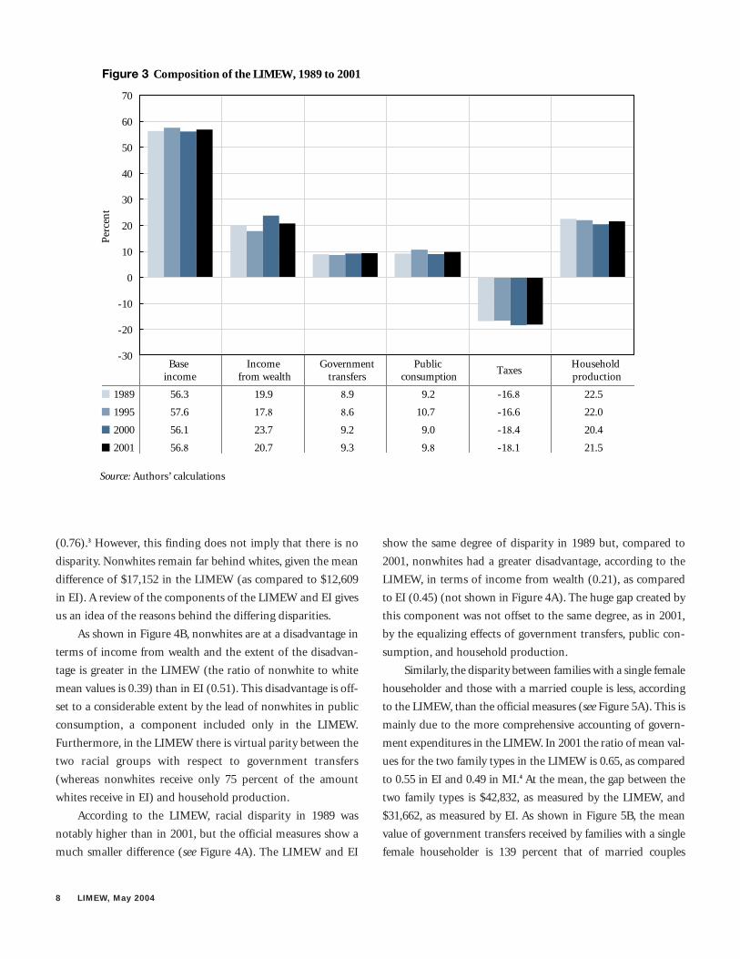
The composition of the LIMEW for various years is shown

in Figure 3. Notable year-to-year fluctuations exist for the income

from wealth component. After falling from 19.9 percent in

1989 to 17.8 percent in 1995, it surged to 23.7 percent in 2000,

before retreating to 20.7 percent in 2001. The fluctuations

largely reflect movements in stock prices, particularly the bull

market of the late 1990s and the stock market collapse in 2001.

Net government expenditures peaked at 3.4 percent in 1995

and bottomed at –0.3 percent in 2000. Although positive in

2001, these expenditures were still below their 1989 level, as a

percentage of the LIMEW and in absolute terms (see Table 3),

because of a higher tax burden. The share of household pro-

duction fell from 22.5 percent in 1989 to 20.4 percent in 2000,

before rising to 21.5 percent in 2001.

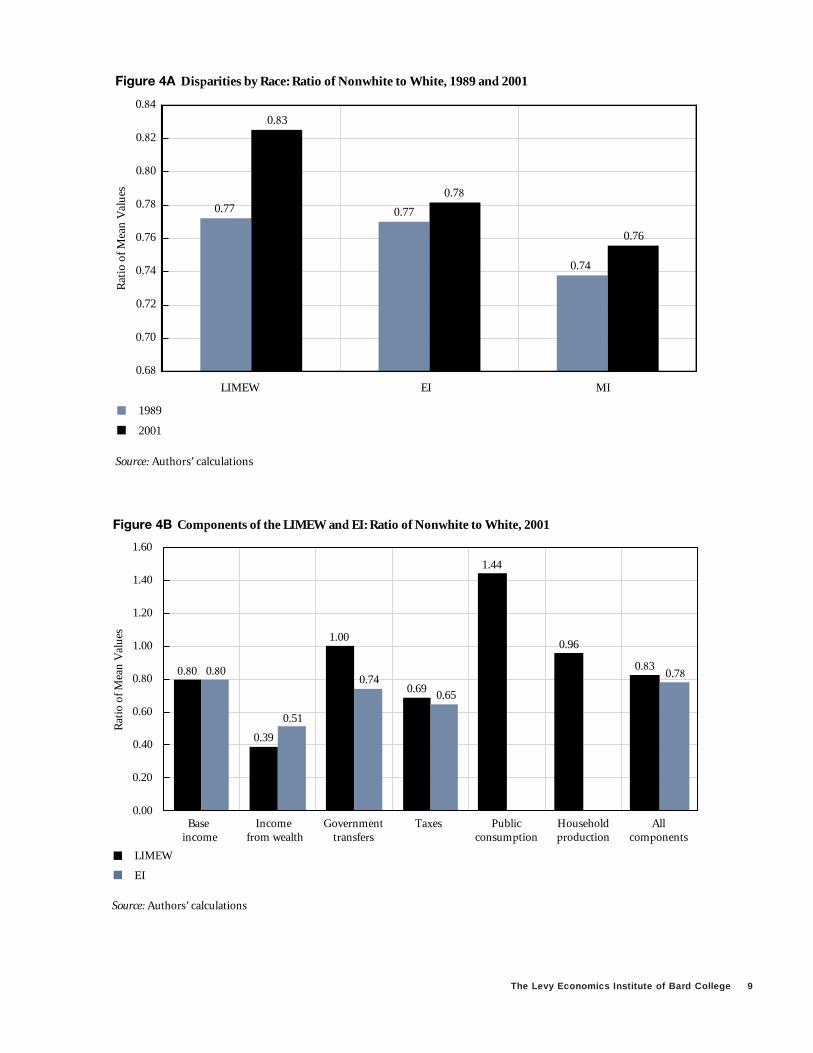
Disparities in Economic Well-Being

The extent of the disparities among households grouped

according to salient social and economic characteristics and the

ways in which these disparities change over time depend on the

yardstick used for measuring well-being. Each bar in Figure 4A

represents a ratio of mean values using the LIMEW, EI, or MI.

In 2001 the racial disparity between nonwhites and whites2 is

less using the LIMEW (0.83), as compared to EI (0.78) and MI

Table 3 Contribution to the Change in Economic Well-Being, 1989 and 2001

Mean Values in 2001 Dollars

LIMEW Extended Income (EI)

Contribution Contribution to change to change

1989 2001 (in percent) 1989 2001 (in percent)

Base income 45,047 53,185 10.2 45,047 53,185 17.1

Income from wealth 15,961 19,383 4.3 8,662 8,567 -0.2

Net government expenditures 1,019 867 -0.2 -6,129 -7,399 -2.7

Transfers 7,137 9,157 2.5 5,699 6,559 1.8

Public consumption 7,343 8,697 1.7

Taxes -13,461 -16,986 -4.4 -11,829 -13,958 -4.5

Household production 18,053 20,160 2.6

Total 80,080 93,595 16.9 47,579 54,353 14.2

Addendum:

Money income 50,981 58,213 14.2


8 LIMEW, May 2004

(0.76).3 However, this finding does not imply that there is no

disparity. Nonwhites remain far behind whites, given the mean

difference of $17,152 in the LIMEW (as compared to $12,609

in EI). A review of the components of the LIMEW and EI gives

us an idea of the reasons behind the differing disparities.

As shown in Figure 4B, nonwhites are at a disadvantage in

terms of income from wealth and the extent of the disadvan-

tage is greater in the LIMEW (the ratio of nonwhite to white

mean values is 0.39) than in EI (0.51). This disadvantage is off-

set to a considerable extent by the lead of nonwhites in public

consumption, a component included only in the LIMEW.

Furthermore, in the LIMEW there is virtual parity between the

two racial groups with respect to government transfers

(whereas nonwhites receive only 75 percent of the amount

whites receive in EI) and household production.

According to the LIMEW, racial disparity in 1989 was

notably higher than in 2001, but the official measures show a

much smaller difference (see Figure 4A). The LIMEW and EI

show the same degree of disparity in 1989 but, compared to

2001, nonwhites had a greater disadvantage, according to the

LIMEW, in terms of income from wealth (0.21), as compared

to EI (0.45) (not shown in Figure 4A). The huge gap created by

this component was not offset to the same degree, as in 2001,

by the equalizing effects of government transfers, public con-

sumption, and household production.

Similarly, the disparity between families with a single female

householder and those with a married couple is less, according

to the LIMEW, than the official measures (see Figure 5A). This is

mainly due to the more comprehensive accounting of govern-

ment expenditures in the LIMEW. In 2001 the ratio of mean val-

ues for the two family types in the LIMEW is 0.65, as compared

to 0.55 in EI and 0.49 in MI.4 At the mean, the gap between the

two family types is $42,832, as measured by the LIMEW, and

$31,662, as measured by EI. As shown in Figure 5B, the mean

value of government transfers received by families with a single

female householder is 139 percent that of married couples

Per

cen

t

-30

-20

-10

0

10

20

30

40

50

60

70

Public consumption

Base income

Income from wealth

Governmenttransfers

TaxesHousehold production

1989 56.3 19.9 8.9 9.2 22.5

1995 57.6 17.8 8.6 10.7 22.0

2000 56.1 23.7 9.2 9.0 20.4

2001 56.8 20.7 9.3 9.8 21.5

-16.8

-16.6

-18.4

-18.1

Figure 3 Composition of the LIMEW, 1989 to 2001



Figure 4B Components of the LIMEW and EI: Ratio of Nonwhite to White, 2001

Rat

io o

f Mea

n V

alu

es

EI

LIMEW

0.00

0.20

0.40

0.60

0.80

1.00

1.20

1.40

1.60

Base income

Income from wealth

Governmenttransfers

Taxes Publicconsumption

Householdproduction

Allcomponents


0.80

0.39

1.00

0.69

1.44

0.96

0.830.80

0.51

0.740.65

0.78

Figure 4A Disparities by Race: Ratio of Nonwhite to White, 1989 and 2001

LIMEW EI MI

Rat

io o

f Mea

n V

alu

es

0.77 0.77

0.74

0.83

0.78

0.76

0.68

0.70

0.72

0.74

0.76

0.78

0.80

0.82

0.84

2001

1989


according to the LIMEW (and 94 percent according to EI). This

component, therefore, has a larger equalizing effect in the

LIMEW. Public consumption is another equalizing factor that

reduces disparity in the LIMEW (with a ratio of 1.38).5

Other household groupings, by age or income, also show

that economic disparity may differ substantially among the vari-

ous measures. The disparity between elderly and average house-

holds is greatest according to MI (0.60) and least according to the

LIMEW (0.95) (see Figure 6A).6 The hump-like shape of the age-

income relationship (i.e., the 35- to 64-year-old group is better

off, while the youngest and oldest age groups are worse off, com-

pared to the average) appears to be indifferent to the measure.

According to the LIMEW (in contrast to EI), the elderly

appear to be almost on par with the average household. The

difference stems mainly from the manner in which income

from wealth is reckoned in the two measures (see Table 1). The

LIMEW includes, as income, the annuity value from nonhome

wealth, which can be quite high for the elderly, owing to a

greater amount of accumulated wealth and a shorter remaining

life expectancy. As a result, the wealth advantage of the elderly

is more prominent in the LIMEW (179 percent of the average

household) than in EI (133 percent) (see Figure 6B).

Also according to the LIMEW, elderly households were

slightly better off than average households in 1989, but the

situation reversed in 2001. The deterioration is due mostly to

changes in income from wealth and government transfers. In

1989 the mean values for elderly households were 227 percent

and 268 percent of average households, respectively (results not

shown). In 2001 the corresponding figures were 179 percent

and 264 percent. The elderly to average household ratios were

more or less the same for the other components.

The disparities among households according to the LIMEW

appear smaller when they are grouped according to money

income in 2001 dollars (see Figure 7A).7 For example, the

$75,000 to $100,000 income group in 2001 is 28 percent better

off than the average household, but 39 percent better off accord-

ing to EI.8 The smaller disparity in the LIMEW is due mainly

to the incorporation of public consumption and household

10 LIMEW, May 2004

Figure 5A Disparities by Family Type, 1989 and 2001

LIMEW EI MI

Rat

io o

f Mea

n V

alu

es


1989

2001

0.77

0.65

0.82

0.57

0.81

0.51

0.72

0.65

0.70

0.55

0.68

0.49

0.00

0.10

0.20

0.30

0.40

0.50

0.60

0.70

0.80

0.90

Single male/married couple

Single female/marriedcouple






Figure 6A Disparities by Age, 2001

Rat

io o

f Mea

n V

alu

es


Less

tha

n 3

5/A

ll

35 t

o 50

/All

51 t

o 64

/All

65 o

r ol

der/

All

Less

tha

n 3

5/A

ll

35 t

o 50

/All

51 t

o 64

/All

65 o

r ol

der/

All

Less

tha

n 3

5/A

ll

35 t

o 50

/All

51 t

o 64

/All

65 o

r ol

der/

All

0.00

0.20

0.40

0.60

0.80

1.00

1.20

1.40

LIMEW EI MI

0.78

1.10 1.12

0.95

0.84

1.16 1.14

0.77

0.87

1.211.18

0.60


EI

LIMEW

Figure 5B Components of the LIMEW and EI: Ratio of Families with Female Householder to Married Couple Families, 2001

Rat

io o

f Mea

n V

alu

es

0.00

0.20

0.40

0.60

0.80

1.00

1.20

1.40

1.60

Base income

Income from wealth

Governmenttransfers


Householdproduction

Allcomponents

0.48

0.37

1.39

0.37

1.38

0.600.65

0.48

0.36

0.94

0.30

0.55

production (see Figure 7B). In addition, there is, presumably, a

small effect from government transfers, since the ratio of mean

values in the LIMEW (0.53) is smaller than in EI (0.61).

Economic Inequality

The official measures and the LIMEW indicate that the distri-

bution of economic well-being, as measured by the Gini coef-

ficient,9 was more unequal in 2001 than in 1989 (see Figure 8).

The official measures show a greater increase in equality between

the two years (4.2 percentage points in EI and 3.7 in MI) than

does the LIMEW (2.0). A comparison between 1995 and 2001,

however, shows that inequality in distribution, as measured by

the LIMEW, grew by a much greater extent (2.3 percentage

points) than either MI (0.6) or EI (1.9). While MI, the most

widely used official measure, suggests that inequality has

hardly changed in the second half of the 1990s, the other meas-

ures point toward an increase in inequality.

As noted earlier, LIMEW–C, EI, and MI are measures that

approximate the magnitude of command over commodities.

Our estimates demonstrate that the level of inequality shown

by the LIMEW–C is substantially higher than that shown by EI

(by a difference of 5.4 percentage points in 2001). With the

exception of 1995, the LIMEW–C shows the highest degree of

inequality, suggesting that the official measures may understate

inequality in the distribution of command over commodities.

In the period from 1995 to 2001, the growth in inequality was

also highest (3 percentage points) using the LIMEW–C measure.

Public consumption and household production are, rela-

tively, more equally distributed. Hence, their inclusion in an

income measure generally lowers the degree of inequality. PFI,

our measure that includes public consumption in addition to the

command over commodities, has a higher level of inequality

than EI, surprisingly, and the difference is considerable (1.8 per-

centage points in 2001). What is not surprising is the much lower

degree of inequality shown in PFI than that which appears in

MI. Similarly, the degree of inequality in distribution shown by

the LIMEW, which also includes household production, is, sur-

prisingly, not that different from that shown by EI in 1995 or

2001, but is conspicuously higher in 1989 and 2000. As

expected, the LIMEW shows more equality in distribution than

does MI.

Compared to the LIMEW, MI overstates inequality because

it is a pretax measure that does not fully account for government

12 LIMEW, May 2004


Figure 6B Components of the LIMEW and EI: Ratio of Elderly to All, 2001

Rat

io o

f Mea

n V

alu

es

0.00

0.50

1.00

1.50

2.00

2.50

3.00

3.50

Base income

Income from wealth

Governmenttransfers


Householdproduction

Allcomponents

0.31

1.79

2.64

0.44 0.40

0.88 0.95

0.31

1.33

3.05

0.42

0.77

EI

LIMEW


Figure 7A Disparities by Income, 2001

Rat

io o

f Mea

n V

alue

s


0.00

0.50

1.00

1.50

2.00

2.50

3.00

3.50

Less

than

$20

k/A

ll

$20k

to $

50k/

All

$50k

to $

75k/

All

$75k

to $

100k

/All

$100

k or

mor

e/A

ll

Less

than

$20

k/A

ll

$20k

to $

50k/

All

$50k

to $

75k/

All

$75k

to $

100k

/All

$100

k or

mor

e/A

ll

Less

than

$20

k/A

ll

$20k

to $

50k/

All

$50k

to $

75k/

All

$75k

to $

100k

/All

$100

k or

mor

e/A

ll

LIMEW EI MI

2.30

0.66

2.61

0.58

2.89

1.47

1.05

1.39

1.06

0.27

0.71

1.28

1.01

0.48

0.19

Figure 7B Components of the LIMEW and EI: Ratio of $75,000–100,000 Income Group to All, 2001

Rat

io o

f Mea

n V

alu

es

0.00

0.40

0.20

0.80

0.60

1.00

1.20

1.40

1.60

1.80

Base income

Income from wealth

Governmenttransfers


Householdproduction

Allcomponents

1.56

1.14

0.53

1.51

1.181.26 1.28

1.56

1.17

0.61

1.55

1.39

EI

LIMEW


transfers and excludes public consumption and household pro-

duction. EI, on the other hand, requires a more complex com-

parison with the LIMEW. The degree of inequality is similar in

the two measures in 1995 and 2001, but quite different in 1989

and 2000 (when the LIMEW is higher). What accounts for the

different pattern?

The overall degree of inequality in an income measure can

be expressed in terms of the “contributions” of its individual

components (Lerman 1999). A component’s contribution can

be calculated as the product of its concentration coefficient and

its share of total income (Yao 1999, pp.1252–53).10 In order to

highlight the role of components, it is convenient to divide

their contribution by the overall degree of inequality and express

the result as a percentage of total inequality. Table 4 shows the

estimated shares of the major components in the overall

inequality of the LIMEW and EI.

First, we consider the difference in the composition of

inequality of EI between 1989 and 1995. The shares of income

from wealth and net government expenditures are lower (in

absolute value) in 1995 and, in tandem the share of base income

is higher. The same pattern holds for EI in 2000 and 2001. Next,

we observe similar compositional change between 1989 and

1995 for the inequality in the LIMEW. However, the composi-

tional change between 2000 and 2001 results in a decline for the

income from wealth component, in favor of base income, net

government expenditures, and household production.

What appears to be common between the LIMEW and EI,

in terms of compositional change between years, is a shift in

favor of base income and away from income from wealth.

However, similar compositional changes were accompanied by

diametrically opposite changes in overall inequality. Inequality

in EI was higher in 1995 and 2001 than it was in 1989 and 2000,

respectively. The converse is true for the LIMEW.

This kind of outcome occurs when the same component

has very different incremental effects on inequality in two dif-

ferent income measures. The incremental effect of a particular

component is the percentage change in overall inequality that

would occur if every household’s income from that component

were to change by 1 percent, assuming other factors remain the

same. If the incremental effect of a component were to increase

14 LIMEW, May 2004

1989

1995

2000

2001

Note: For definitions, see Table 1 and notes to Table 2.


Figure 8 Economic Inequality by Income Measure, 1989 to 2001

Gin

i Coe

ffic

ien

t x

100

0

10

20

30

40

50

60

38.9 44.2 41.0 36.9 41.8

38.6 43.5 40.5 39.2 44.9

42.5 48.9 45.0 40.8 46.0

40.9 46.5 42.9 41.1 45.5

LIMEW LIMEW-C PFI EI MI

tion in the share of these expenditures contributed to higher

inequality in 1995 and 2001, as compared to 1989 and 2000,

respectively.

Net government expenditures have a smaller negative

incremental effect (-12.8 percent) on inequality in the LIMEW.

An increase in the share of net government expenditures in

2001, relative to 2000, contributed, therefore, to the decline in

inequality. Household production (excluded from the EI), with

its small negative incremental effect (-2.0 percent) contributed

to lower inequality of the LIMEW in 1995 and 2001, as com-

pared to 1989 and 2000, respectively.

A closer look at the composition of inequality and the

incremental effects of individual components suggests that,

although the LIMEW and EI display approximately the same

degree of inequality in 2001, the implications differ. Policy con-

siderations are often informed by the incremental effect of

variables and, as already discussed, the two measures are sig-

nificantly different in this respect.

Earnings, which make up the overwhelming portion of base

income, are the decisive factor shaping the overall level of

inequality in EI. But they represent a much smaller portion of

inequality in the LIMEW. The difference suggests that to consider

inequality, we would expect inequality to be higher than it

would otherwise be if the component’s share in inequality were

to increase. The incremental effects were similar for all years.

Therefore, only 2001, the most recent year for which estimates

are available, is shown in Figure 9.

The incremental effects of the base-income and income-

from-wealth components on inequality are strikingly different

in the LIMEW and EI. In fact, the components’ roles are reversed

in the two measures. Base income has a large positive effect on

inequality (16.6 percent) in EI and a small negative effect (-1.2

percent) in the LIMEW. Conversely, income from wealth has a

large positive effect on inequality (16.0 percent) in the LIMEW

and a much smaller effect (5.7 percent) in EI.

Changes in the share of other components in the two

measures further reinforced the opposing effects on inequality

from the compositional change in favor of base income and

against income from wealth. There was a reduction in the

share of net government expenditures in the inequality of EI in

later years (i.e., the share in 1995 and 2001 was lower than in

1989 and 2000, respectively). As is shown in Figure 9, net gov-

ernment expenditures have a strong negative incremental

effect (-22.2 percent) on inequality in EI. Therefore, the reduc-


Table 4 Shares of Income Components in Inequality by Income Measure, 1989-2001 (in percent)

LIMEW Extended Income (EI)

1989 1995 2000 2001 1989 1995 2000 2001

Base income 53.2 58.7 51.8 55.6 111.1 112.0 112.4 114.4

Income from wealth 37.1 31.4 42.0 36.7 26.1 21.8 23.8 21.4

Net government expenditures -11.4 -11.2 -11.4 -11.9 -37.3 -33.9 -36.2 -35.8

Household production 21.0 21.1 17.7 19.5

Total 100.0 100.0 100.0 100.0 100.0 100.0 100.0 100.0

Addendum:

Gini coefficient x 100 38.9 38.6 42.5 40.9 36.9 39.2 40.8 41.1

Note: The contribution of a given income component (k) is calculated as the product of its concentration coefficient (Ck) and its share in total income (S yk ), with

appropriate modification to allow population weighting. The share of an income component in inequality (S lk ) is calculated as the contribution of that compo-

nent divided by the overall Gini coefficient. Let the population weight of the i th household be wi and the total number in the sample be equal to n. Also, let yki

denote the amount of income component k for the i th household, and yi its total income. Then,

Ck = 1- nΣ

i=1pi(2Qki -ski ), where pi = wi/

nΣ

i=1wi , ski = yki wi /

nΣ

i=1yki wi , and, Qki =

iΣ

j=1skj.

The share of an income component in total income is calculated as: S yk =

nΣ

i=1ykiwi/

nΣ

i=1yiwi . It should be noted that the households in the sample are sorted in ascend-

ing order of y before Ck is calculated. The incremental effect referred to in the text is calculated as (S lk - S y

k ).


economic inequality as shaped, basically, by earnings inequal-

ity may be misleading. Wealth inequality also plays an impor-

tant role.

Net government expenditures considerably reduce the over-

all level of inequality in the LIMEW and EI. The share of net

government expenditures is negative and large (see Table 4).

However, the effect of net government expenditures is much

larger (-35.8 percent in 2001) in EI as compared to the LIMEW

(-11.9 percent). The same relationship also holds with respect to

the incremental effects on inequality that were noted earlier (see

Figure 9). Thus, the share and the incremental effect of net

government expenditures in inequality appear to be overstated

in EI, as compared to the LIMEW. Furthermore, the incremental

effect of taxes and expenditures on the degree of inequality are

different in the LIMEW and EI. The EI suggests that taxes and

expenditures have similar incremental effects (see Figure 10). In

contrast, the LIMEW suggests that expenditures have a markedly

higher incremental effect in reducing inequality than do taxes.

The main difference between the two measures with regard

to income from wealth is the treatment of nonhome wealth. As

shown in Figure 11, the incremental effect of imputed income

from housing wealth has a broadly similar effect in both meas-

ures—a small inequality-reducing effect (-1.9 percent) in EI

and a neutral effect (0.4 percent) in the LIMEW. At the mar-

gin, therefore, whether the advantage from homeownership is

reckoned in terms of an imputed return on net home equity, as

in EI, or as an imputed rental cost, as in the LIMEW, seems to

have little bearing on inequality. In contrast, the inequality-

enhancing effect of imputed income from nonhome wealth in

the LIMEW is twice that in EI (15.6 percent, as compared to 7.5

percent). Thus, whether nonhome wealth is treated as a lifetime

annuity on net worth, as in the LIMEW, or as current realized

income from assets, as in EI, has a substantial impact on

inequality.

Conclusion

Any picture of economic well-being is crucially dependent on

the yardstick used to measure it. Admittedly, gross money income

(MI), the most widely used official measure, may be suitable

for certain purposes. But it is an incomplete measure in several

important ways. The elevation of more comprehensive

income measures to a status that is on par with MI in the official

scorecard of the economic well-being of U.S. households is a

16 LIMEW, May 2004

Figure 10 Incremental Effects of Government Expendituresand Taxes on Inequality in the LIMEW and EI, 2001

Per

cen

t

-14.0

-12.0

-10.0

-8.0

-6.0

-4.0

-2.0

0.0

Government expenditures TaxesLIMEW

EI

See the note to Table 4 for the formulas used to calculate the incremental effects.


-1.4

-12.2

-10.1

-11.5

Figure 9 Incremental Effects of the Components of Income on Inequality in the LIMEW and EI, 2001

Per

cen

t

LIMEWEI

15.0

10.0

5.0

0.0

-5.0

-10.0

-15.0

-20.0

-25.0

20.0

Base income

Income from wealth

Net governmentexpenditures

Householdproduction

-1.2

16.0

-2.0

16.6

5.7

-22.2

-12.8



Disparities among population subgroups are generally

lower according to the LIMEW as compared to other measures.

For example, the racial gap in well-being in 2001 appears to be

much smaller in the LIMEW assessments. The narrowing of the

racial gap also appears to occur at a higher rate according to the

LIMEW. The lower racial gap, relative to EI measures, is trace-

able, mainly, to the higher degree of public consumption by

nonwhites and to the near parity in household production.

Disparities are generally lower among age groups and house-

holds grouped by income in the LIMEW than in either MI or

EI. The elderly, in particular, are much better off, according to

the LIMEW, because of greater income from wealth. Our results

suggest that the relevant action, both analytically and in terms

of public policy, would be to investigate the forces behind the

disparities. We plan to address this in future research.

Differences with respect to which components are selected

and how they are included in the measure of well-being also

play a crucial role in the analysis of overall economic inequal-

ity. While two income measures might show the same degree of

inequality (e.g., the LIMEW and EI in 2001), the structure of

the inequality may be radically different. Our analysis of the

incremental effects of individual components on inequality

suggests that base income (primarily earnings), has a large


sure indication that academic discussion and policy making will

be increasingly informed by such measures.

The LIMEW is different in scope from the official measures.

It recognizes that economic well-being depends on public and

self provisioning, in addition to the command over commodi-

ties. In contrast the official measures are restricted to measuring

the command over commodities. There is no unanimity among

economists and policy makers as to how to incorporate public

consumption and household production into measures of eco-

nomic well-being. A consensus is unlikely to emerge in the

immediate future, given the length of time since these compo-

nents entered discussions of well-being. Because we believe that

these components are important in evaluating economic well-

being, we have developed a set of estimates that reflect their effect

and significance. Since the production of estimates is contingent

on developing an information base, we accomplish two goals

simultaneously. One, we calculate a set of estimates that gives a

concrete picture of the level, composition, and distribution of

public consumption and household production. Two, the infor-

mation base allows us to perform sensitivity analyses of alterna-

tive assumptions. The results of these analyses will be reported in

future LIMEW publications of the Levy Institute.

The LIMEW also differs from the official measures in its

methods, especially its treatment of income from wealth and

noncash transfers (see Table 1). These differences are more than

formulaic; they are the result of alternative concepts of eco-

nomic well-being (Wolff, Zacharias, and Caner 2004, 7:9; Wolff

and Zacharias 2002).

The differences in scope and method lead to substantially

different findings regarding economic well-being. The median

U.S. household appears to be much better off in 2001 than in

1989, according to the LIMEW. However, the increase in well-

being was accompanied by a considerable increase in the total

annual hours worked by the median household—the rate of

increase between 1989 and 2001, according to one estimate,

exceeded MI figures and was close to EI figures. While mean val-

ues of the LIMEW and official measures display similar rates of

change, the median values of the LIMEW show a much faster

growth rate than the comparable values of the official measures.

This discrepancy, between rates of change in mean and median

values, most likely reflects the fact that the LIMEW includes pub-

lic consumption and household production. These two compo-

nents are large and relatively equally distributed, compared to

other components of the LIMEW and the official measures.


Figure 11 Incremental Effects of Home and Nonhome Wealth on Inequality in the LIMEW and EI, 2001

Per

cen

t

-2.0

-4.0

0.0

2.0

4.0

6.0

8.0

10.0

12.0

14.0

16.0

18.0

Home NonhomeLIMEWEI


0.4

15.6

-1.9

7.5

inequality-enhancing effect on EI and a small inequality-

reducing effect on the LIMEW. In sharp contrast, the incre-

mental effect of income from wealth on increasing inequality is

much higher in the LIMEW than in EI. Similarly, while net

government expenditures have an inequality-reducing effect

for both measures, EI overstates the effect, as compared to the

LIMEW. A more important observation, from a policy stand-

point, is the asymmetric incremental effect of taxes on inequal-

ity when the two measures are compared. Taxes have a large

negative effect that is similar to government spending in EI,

while, in the LIMEW, government spending appears to have a

much larger inequality-reducing effect than do taxes.

Several issues related to economic well-being require fur-

ther research and evaluation. We hope that our analysis will

lead to further academic and policy research and will stimulate

a rethinking of public policies that affect well-being.

Acknowledgments

We gratefully acknowledge the helpful comments and advice

of Dimitri Papadimitriou, Thomas Hungerford, and Rania

Antonopoulos of the Levy Institute, as well as the able research

assistance of Melissa Mahoney. We have also benefited from

comments by Sheldon Danziger, Peter Gottschalk, Stephen

Jenkins, David Levine, Lars Osberg, Juliet Schor, and Daniel

Weinberg. We appreciate the comments from the Levy

Economics Institute seminar participants.

Notes

1. In order to be consistent with our estimates of weekly

hours of housework, we have chosen to report the annual

hours of paid work based on our imputed weekly hours

of paid work in Table 2 and Figure 2. Because the time-

use surveys do not have estimates of weeks worked per

year, we calculated the annual hours of paid work by mul-

tiplying the imputed weekly hours of paid work by the

weeks worked per year, as reported in the ASEC. If we

were to use the weekly hours of paid work reported by the

ASEC, along with the imputed weekly hours of house-

work, we might end up with improbable values for weekly

hours of total work.

2. “Whites” refers to non-Hispanic whites only. “Nonwhites”

refers to everyone else.

3. The ratios of median values are, in general, close to the

ratios of mean values. In 2001, the ratios are 0.88 for the

LIMEW, 0.77 for EI, and 0.75 for MI. We prefer to use the

ratio of means because it allows us to decompose the over-

all disparities into disparities in individual components.

4. The ratios of median values are similar. In 2001 they are

0.68 for the LIMEW, 0.55 for EI, and 0.46 for MI.

5. It is interesting to note that, while disadvantage in well-

being faced by single female householder families was the

same in 2001 and 1989, single male householder families

fell further behind married couples in 2001, as compared

to 1989, by all three income measures.

6. The ratios of median values in 2001 are 0.84, 0.77, and

0.55, according to the LIMEW, EI, and MI, respectively.

7. Since households are classified into groups according to

MI, disparities will be lower in measures other than MI.

The surprising finding, however, is how much the dis-

crepancies are reduced by using the LIMEW.

8. The ratios of median values are in general higher than the

ratios of mean values. In 2001, they are 1.50, 1.73, and

2.02, according to the LIMEW, EI, and MI, respectively.

9. The Gini coefficient is an index that ranges from zero

(perfect equality) to one (maximal inequality). To facilitate

exposition, we use values that are 100 times the Gini coef-

ficient. We also estimate the Atkinson measures of

inequality, but they are not reported here, because our

arguments about the level of and changes in inequality

seem to be valid with either measure.

10. The concentration coefficient is similar to the Gini coeffi-

cient. The Gini coefficient is the area between the Lorenz

curve and the 45-degree line multiplied by 2, while the

concentration coefficient is the area between the concen-

tration curve and the 45-degree line multiplied by 2. The

Lorenz curve plots the cumulative proportion of income

on the vertical axis and the cumulative proportion of

households on the horizontal axis, with the cumulative

proportions calculated after households are ordered accord-

ing to income (starting from the lowest and ending with

the highest). If we were to plot the cumulative proportion

of a component of income (e.g., wages), keeping the same

ordering of households on the horizontal axis, the curve

connecting all points plotted would be the concentration

curve for that component.

18 LIMEW, May 2004

References

DeNavas-Walt, Carmen, Robert Cleveland, and Bruce H.

Webster Jr. 2003. U.S. Census Bureau, Current Population

Reports, P60-221, Income in the United States, U.S.

Government Printing Office: Washington, D. C.

Lerman, Robert I. 1999. “How Do Income Sources Affect

Income Inequality?” Handbook on Income Inequality

Measurement, Jacques Silber, ed. pp. 341–58. Boston:

Kluwer Academic Publishers.

Wolff, Edward N., Ajit Zacharias, and Asena Caner. 2004.

“Levy Institute Measure of Economic Well-Being,

Concept, Measurement and Findings: United States, 1989

and 2000.” February. Annandale-on-Hudson, N.Y.: The

Levy Economics Institute.

Wolff, Edward N. and Ajit Zacharias. 2002. “The Levy Institute

Measure of Economic Well-Being.” Unpublished manu-

script. October. The Levy Economics Institute.

Yao, Shujie. 1999. “On the Decomposition of Gini Coefficients

by Population Class and Income Source: A Spreadsheet

Approach and Application.” Applied Economics, vol. 31,

pp. 1249–64.

Related Levy Institute Publications

Levy Institute Measure of Economic Well-Being

Concept, Measurement, and Findings: United States, 1989

and 2000


February 2004

Levy Institute Measure of Economic Well-Being

United States, 1989 and 2000


December 2003

Asset Poverty in the United States

Its Persistence in an Expansionary Economy

asena caner and edward n. wolff

Public Policy Brief No. 76, 2004 (Highlights, No. 76A)

Inequality of the Distribution of Personal Wealth in

Germany 1973–1998

richard hauser and holger stein

Working Paper No. 398, January 2004

The Evolution of Wealth Inequality in Canada, 1984–1999

rené morissette, xuelin zhang, and marie drolet

Working Paper No. 396, November 2003

On Household Wealth Trends in Sweden over the 1990s

n. anders klevmarken


Wealth Transfer Taxation: A Survey

helmuth cremer and pierre pestieau


Other Levy Institute Publications

POLICY NOTES

Inflation Targeting and the Natural Rate of Unemployment

willem thorbecke

2004/1

The Future of the Dollar: Has the Unthinkable Become

Thinkable?

korkut a. ertürk

2003/7

Is International Growth the Way Out of U.S. Current

Account Deficits? A Note of Caution

anwar m. shaikh, gennaro zezza,

and claudio h. dos santos

2003/6

Deflation Worries

l. randall wray

2003/5

PUBLIC POLICY BRIEFS

Is Financial Globalization Truly Global?

New Institutions for an Inclusive Capital Market

philip arestis and santonu basu

No. 75, 2003 (Highlights, No. 75A)

Understanding Deflation

Treating the Disease, Not the Symptoms

l. randall wray and dimitri b. papadimitriou



Asset and Debt Deflation in the United States

How Far Can Equity Prices Fall?

philip arestis and elias karakitsos


What Is the American Model Really About?

Soft Budgets and the Keynesian Devolution

james k. galbraith


Can Monetary Policy Affect the Real Economy?

The Dubious Effectiveness of Interest Rate Policy

philip arestis and malcolm sawyer


STRATEGIC ANALYSES

Is Deficit-Financed Growth Limited? Policies and Prospects

in an Election Year

dimitri b. papadimitriou, anwar m. shaikh,

claudio h. dos santos, and gennaro zezza

April 2004

Deficits, Debts, and Growth: A Reprieve But Not a Pardon

anwar m. shaikh, dimitri b. papadimitriou,

claudio h. dos santos, and gennaro zezza

October 2003

WORKING PAPERS

Some Simple, Consistent Models of the Monetary Circuit

gennaro zezza

No. 405, April 2004

The “War on Poverty” after 40 Years:

A Minskyan Assessment

stephanie a. bell and l. randall wray

No. 404, April 2004

A Stock-Flow Consistent General Framework for Formal

Minskyan Analyses of Closed Economies

claudio h. dos santos

No. 403, February 2004

A Post-Keynesian Stock-Flow Consistent Macroeconomic

Growth Model: Preliminary Results

claudio h. dos santos and gennaro zezza

No. 402, February 2004

Borrowing Alone: The Theory and Policy Implications of the

Commodification of Finance

greg hannsgen

No. 401, January 2004

Fiscal Consolidation: Contrasting Strategies & Lessons from

International Experiences

jörg bibow


Does Financial Structure Matter?

philip arestis, ambika d. luintel, and

kul b. luintel


This LIMEW publication and all other Levy Institute publi-

cations are available online on the Levy Institute website,

www.levy.org.

To order a Levy Institute publication, call 845-758-7700 or

202-887-8464 (in Washington, D.C.), fax 845-758-1149,

e-mail [email protected], write The Levy Economics Institute of

Bard College, Blithewood, PO Box 5000, Annandale-on-

Hudson, NY 12504-5000, or visit our website at www.levy.org.

20 LIMEW, May 2004

NONPROFIT ORGANIZATION

U.S. POSTAGE PAID

BARD COLLEGE

The Levy Economics Institute of Bard College

Blithewood

PO Box 5000

Annandale-on-Hudson, NY 12504-5000

Address Service Requested

Levy Institute Measure of Economic Well-Being Levy Economics Institute of Bard College 3 Preface...

Documents

Transcript of Levy Institute Measure of Economic Well-Being Levy Economics Institute of Bard College 3 Preface...