Level-set topology optimization with many linear buckling ... · PDF fileslow convergence and...
25
INTERNATIONAL JOURNAL FOR NUMERICAL METHODS IN ENGINEERING Int. J. Numer. Meth. Engng (2016) Published online in Wiley Online Library (wileyonlinelibrary.com). DOI: 10.1002/nme.5203 Level-set topology optimization with many linear buckling constraints using an efficient and robust eigensolver Peter D. Dunning 1, * ,† , Evgueni Ovtchinnikov 2 , Jennifer Scott 2 and H. Alicia Kim 3 1 School of Engineering, University of Aberdeen, Aberdeen AB24 3UE, UK 2 Scientific Computing Department, STFC Rutherford Appleton Laboratory, Didcot Oxfordshire OX11 0QX, UK 3 Structural Engineering Department, University of California, San Diego, USA SUMMARY Linear buckling constraints are important in structural topology optimization for obtaining designs that can support the required loads without failure. During the optimization process, the critical buckling eigenmode can change; this poses a challenge to gradient-based optimization and can require the computation of a large number of linear buckling eigenmodes. This is potentially both computationally difficult to achieve and pro- hibitively expensive. In this paper, we motivate the need for a large number of linear buckling modes and show how several features of the block Jacobi conjugate gradient (BJCG) eigenvalue method, including opti- mal shift estimates, the reuse of eigenvectors, adaptive eigenvector tolerances and multiple shifts, can be used to efficiently and robustly compute a large number of buckling eigenmodes. This paper also introduces linear buckling constraints for level-set topology optimization. In our approach, the velocity function is defined as a weighted sum of the shape sensitivities for the objective and constraint functions. The weights are found by solving an optimization sub-problem to reduce the mass while maintaining feasibility of the buckling constraints. The effectiveness of this approach in combination with the BJCG method is demonstrated using a 3D optimization problem. Copyright © 2016 John Wiley & Sons, Ltd. Received 3 July 2015; Revised 30 December 2015; Accepted 4 January 2016 KEY WORDS: topology optimization; buckling constraints; level-set method; block conjugate gradient eigensolver; sparse direct linear solver 1. INTRODUCTION The objective of optimum structural design is often to find the lightest structure that can support the loading conditions without failure. There has been extensive research into developing and applying optimization methods to structural design problems [1, 2]. However, structures that are optimized for minimum weight often consist of beam-like members or thin panels. If these types of structure are subjected to compressive loads, then they may be prone to buckling, which ultimately limits the capacity of the structure to carry load. Therefore, it is important to include buckling as a constraint in structural optimization problems. Topology optimization is one approach to design efficient structures that have received significant attention [3, 4]. The idea is to open up the design space such that sizing, shape and connectivity of the structure are considered simultaneously, leading to the greatest design freedom. Buckling has been considered in both truss and continuum type topology optimization. In truss type topology optimization, the design space typically consists of a fixed set of nodes connected by a large number of pin-jointed truss members, a so-called ground structure. The design variables are usually member cross-sections, which can go to zero to allow a change in topology. Local Euler buckling constraints can be specified on each member, although a modification of the design space *Correspondence to: School of Engineering, University of Aberdeen, Aberdeen AB24 3UE, UK. † E-mail: [email protected] Copyright © 2016 John Wiley & Sons, Ltd.
-
Upload
truongdien -
Category
Documents
-
view
214 -
download
0
Transcript of Level-set topology optimization with many linear buckling ... · PDF fileslow convergence and...
INTERNATIONAL JOURNAL FOR NUMERICAL METHODS IN ENGINEERINGInt. J. Numer. Meth. Engng (2016)Published online in Wiley Online Library (wileyonlinelibrary.com). DOI: 10.1002/nme.5203
Level-set topology optimization with many linear bucklingconstraints using an efficient and robust eigensolver
Peter D. Dunning1,*,† , Evgueni Ovtchinnikov2, Jennifer Scott2 and H. Alicia Kim3
1School of Engineering, University of Aberdeen, Aberdeen AB24 3UE, UK2Scientific Computing Department, STFC Rutherford Appleton Laboratory, Didcot Oxfordshire OX11 0QX, UK
3Structural Engineering Department, University of California, San Diego, USA
SUMMARY
Linear buckling constraints are important in structural topology optimization for obtaining designs that cansupport the required loads without failure. During the optimization process, the critical buckling eigenmodecan change; this poses a challenge to gradient-based optimization and can require the computation of a largenumber of linear buckling eigenmodes. This is potentially both computationally difficult to achieve and pro-hibitively expensive. In this paper, we motivate the need for a large number of linear buckling modes andshow how several features of the block Jacobi conjugate gradient (BJCG) eigenvalue method, including opti-mal shift estimates, the reuse of eigenvectors, adaptive eigenvector tolerances and multiple shifts, can be usedto efficiently and robustly compute a large number of buckling eigenmodes. This paper also introduces linearbuckling constraints for level-set topology optimization. In our approach, the velocity function is defined asa weighted sum of the shape sensitivities for the objective and constraint functions. The weights are foundby solving an optimization sub-problem to reduce the mass while maintaining feasibility of the bucklingconstraints. The effectiveness of this approach in combination with the BJCG method is demonstrated usinga 3D optimization problem. Copyright © 2016 John Wiley & Sons, Ltd.
Received 3 July 2015; Revised 30 December 2015; Accepted 4 January 2016
KEY WORDS: topology optimization; buckling constraints; level-set method; block conjugate gradienteigensolver; sparse direct linear solver
1. INTRODUCTION
The objective of optimum structural design is often to find the lightest structure that can support theloading conditions without failure. There has been extensive research into developing and applyingoptimization methods to structural design problems [1, 2]. However, structures that are optimizedfor minimum weight often consist of beam-like members or thin panels. If these types of structureare subjected to compressive loads, then they may be prone to buckling, which ultimately limits thecapacity of the structure to carry load. Therefore, it is important to include buckling as a constraintin structural optimization problems.
Topology optimization is one approach to design efficient structures that have received significantattention [3, 4]. The idea is to open up the design space such that sizing, shape and connectivity ofthe structure are considered simultaneously, leading to the greatest design freedom.
Buckling has been considered in both truss and continuum type topology optimization. In trusstype topology optimization, the design space typically consists of a fixed set of nodes connectedby a large number of pin-jointed truss members, a so-called ground structure. The design variablesare usually member cross-sections, which can go to zero to allow a change in topology. Local Eulerbuckling constraints can be specified on each member, although a modification of the design space
*Correspondence to: School of Engineering, University of Aberdeen, Aberdeen AB24 3UE, UK.†E-mail: [email protected]
Copyright © 2016 John Wiley & Sons, Ltd.
P. D. DUNNING ET AL.
is often required to handle discontinuities when member areas go to zero [5]. However, the localconstraints may not prevent global buckling of the structure, because of the presence of hinges [6].Thus, a global buckling constraint is also included [7]. For continuum structures, it is difficult toidentify discrete structural members. Therefore, specific local buckling constraints are not used [8].Instead, a linear buckling analysis [8–11] or a geometrically non-linear analysis [8, 12] is used tocompute the critical buckling load. Buckling constraints have been used with several continuumtopology optimization methods including simple isotropic material with penalization [12], evolu-tionary structural optimization [10] and a nodal design variable method [8]. The level-set method isanother approach to continuum topology optimization that has received significant attention in thelast 10 years [3, 4, 13, 14]. However, to the authors knowledge, buckling constraints have not beenincluded in level-set-based topology optimization.
This paper is concerned with the design of continuum structures, where the critical load factoris computed using a linear buckling analysis. The analysis is performed in two steps [15]. The firstsolves a linear elastic problem using standard finite element analysis to obtain displacement andstress values for the given loading. A generalized eigenvalue analysis is then performed, where theeigenvalues are the buckling load factors and the eigenvectors correspond to the buckling modeshapes. This is sometimes known as the buckling eigenvalue problem.
A number of key issues have been identified that can affect the convergence of optimizationproblems involving linear buckling. One issue relates to the computation of buckling load factorderivatives. The geometric or stress stiffness matrix used in the buckling eigenvalue problem isdependent on the displacements from the linear elastic analysis, which are in turn dependent on thedesign variables. However, this contribution to the gradient calculation is sometimes ignored forsimplicity, resulting in some error in the computed gradients [16]. Another issue is that repeatedeigenvalues are only directionally differentiable [17]. Ascent directions in the presence of repeatedeigenvalues can be computed by introducing additional requirements that the directional derivativeof all repeated eigenvalues must be positive [17, 18]. Non-differentiability can be avoided if theproblem is solved using semi-definite programming methods [7], although the addition of matrixconstraints significantly increases the computational cost. Bruyneel et al [16] also discuss how thechoice of optimizer can affect the convergence of buckling constrained problems and show thatthe use of information from two consecutive iterations to approximate the curvature produces anenvelope of the responses and helps find a feasible solution. Moreover, methods that use an internalmove-limit strategy can improve convergence.
Another key issue is the switching of the critical buckling mode during optimization. A constraintis usually posed that the lowest buckling load factor must be greater than one. However, the bucklingmode with the lowest load factor may change during optimization. This introduces a discontinuity,as the mode shape and gradient information of the lowest mode will change, leading to slow con-vergence, or even a failure to converge. Using a greater number of modes provides the optimizerwith more comprehensive information about the design space and can improve the convergence.Bruyneel et al [16] showed, for example, that increasing the number of buckling mode constraintsfrom 12 to 100 reduced the number of iterations to converge from 44 to 6. For realistic structureswith complex topological configurations, such as 3D aircraft wings [19], even more buckling modesmay be required.
Topology optimization methods often use a fictitious weak material to model void regions in thedesign space. The weak material has stiffness and density values several orders of magnitude thanthe real material. This leads to large differences in the diagonal entries of the system matrices (suchas the stiffness matrix) large condition numbers and ill-conditioning [20]. Furthermore, topologyoptimization methods that use the extended finite element (FE) method to model a material-voidinterface can produce ill-conditioned matrices if element integration areas are small [21].
The efficient computation of a large number of buckling load factors and mode shapes forlarge-scale topology optimization problems presents a significant computational challenge, as thesolution of a sequence of generalized eigenvalue problems with ill-conditioned matrices is required.Currently, the most widely used solvers for such problems, such as ARPACK [22] (which is usedby the MATLAB [23] function eigs) and the F12 package from the NAG library [24], employKrylov subspace methods with a shift-and-invert technique. When used to solve a buckling problem,
Copyright © 2016 John Wiley & Sons, Ltd. Int. J. Numer. Meth. Engng (2016)DOI: 10.1002/nme
BUCKLING CONSTRAINED TOPOLOGY OPTIMIZATION
the shift-invert technique requires the user to solve a sequence of large sparse linear systems of theform .A � �B/u D f , where A and B are real symmetric ill-conditioned matrices. At present,such systems can only be reliably solved using a sparse direct solver, such as the HSL_MA97 pack-age [25] from the HSL mathematical software library [26] or the SPRAL_SSIDS package from theSPRAL library [27]. The solution involves two steps: the factorization of A � �B , which must bedone once for each shift � , and the repeated solution of linear systems using the matrix factorization.Although the second step is normally less computationally expensive than the first, it may accountfor a substantial proportion of the eigenvalue computation time if it is performed a large number oftimes, for example, if a large number of eigenvalues are required.
For a fixed shift � , Krylov solvers are theoretically optimal, as they, in a sense, require the min-imal possible number of shifted solves. For this reason, ARPACK remains a highly competitiveeigensolver more than two decades after its introduction. However, there are certain limitationsthat hinder its efficient use. Firstly, even though a Krylov solver can compute several eigenvaluessimultaneously, the shifted systems are solved one after another, limiting the scope for parallel com-putation. Further, Krylov solvers generally cannot reliably compute repeated eigenvalues and maymiss eigenvalues that are close to each other. This is of particular concern to a linear buckling con-strained problem, where the minimum eigenvalue must be greater than one and the optimal designmay have several eigenvalues close to one. If a critical eigenvalue close to one is missed, then theoptimizer does not receive gradient information for the eigenvalue and may change the structuresuch that the eigenvalue becomes infeasible. This can slow down convergence, as the missed modeoscillates between feasible and infeasible. Also, if a critical eigenvalue is missed throughout theoptimization, then the final design may not be feasible if the missed eigenvalue is less than one. Bothslow convergence and infeasible final designs are undesirable in optimization, and thus a solver thatcan guarantee that eigenvalues are not missed is preferred. Part of the reason for ARPACK’s prob-lems with nearly repeated eigenvalues is the fact that ARPACK counts eigenvalues as they converge.The speed of convergence is determined by the relative separation of the computed eigenvalue fromthe rest of the spectrum. As a result, well-separated eigenvalues further down the spectrum that arenot wanted often converge before wanted eigenvalues. In practice, this implies that the user mustforce the convergence to all wanted eigenvalues by using machine accuracy error tolerance, even ifsuch accuracy is not required, and compute more eigenvalues than are needed.
In this paper, we opt for an alternative approach that exploits two time-tested techniques: sub-space, or block, iterations and the conjugate gradient (CG) method. The full details will be givenin Section 3: here, we briefly summarize the advantages of such an approach. The block iterativenature of the proposed eigensolver ensures that all wanted eigenvalues are computed and allows theefficient exploitation of parallel capabilities of modern computer architectures, both via the use ofhighly optimized Level 3 BLAS subroutines and the use of OpenMP for simultaneous shifted solves.We need to solve several increasingly close eigenvalue problems, and our eigensolver enables us toexploit the previously computed eigenvalues and eigenvectors, significantly improving performance.The reliability of block iterations allows the use of a relaxed error tolerance at early outer itera-tions and a reduced tolerance as the iterations proceed. Finally, the use of CG delivers convergencesimilar to that of a block Krylov method (the two are mathematically equivalent when applied to alinear system with a matrix right-hand side [28]) at a considerable reduction in the computationalcost. We note that the block CG approach has been successfully used by several authors in combi-nation with preconditioning techniques [29, 30]. However, their experiments have been performedusing research software that is not be of library quality in terms of robustness, efficiency and relia-bility. Our new eigensolver package SPRAL_SSMFE, which implements the algorithm described inSection 3, is a fully supported and maintained high-quality implementation that is included withinthe SPRAL software library [27].
The novel contributions of this paper are first, the demonstration, using a clear example that alarge number of eigenmodes in linear buckling constrained optimization may be required for stableconvergence; second, the efficient and robust computation of such modes using the BJCG eigenvaluesolver SPRAL_SSMFE is investigated; and third, a method for including linear buckling constraintsin level-set topology optimization is introduced. The paper is organized as follows. Section 2introduces the buckling constrained minimization of mass problem and the linear buckling
Copyright © 2016 John Wiley & Sons, Ltd. Int. J. Numer. Meth. Engng (2016)DOI: 10.1002/nme
P. D. DUNNING ET AL.
eigenvalue problem. The need for computing a large number of buckling modes is highlighted usinga simple example. The BJCG eigenvalue solver is introduced and discussed in Section 3, and its per-formance is investigated in Section 4. The level-set method with buckling constraints is detailed inSection 5. A 3D topology optimization example is presented in Section 6, followed by conclusionsin Section 7.
2. LINEAR BUCKLING OPTIMIZATION
2.1. Buckling constrained problem
The optimization problem studied in this paper is to minimize the mass of a structure, subject to aconstraint that the lowest positive buckling load factor is greater than or equal to one:
minx
M.x/
s.t. K.x/u D f
ŒK.x/C ˛Ks.x; u/�v D 0
˛1 > 1;
(1)
where x is a vector of design variables, K the structural stiffness matrix, u the displacement vector,f the force vector,Ks the stress stiffness matrix, ˛ a buckling load factor, with ˛1 the lowest positivefactor, and v a buckling mode shape eigenvector. The first two constraints comprise a linear staticequation followed by a buckling eigenvalue problem. Additional constraints on the design variables,x, may also be included. Note that K is symmetric positive definite and Ks is symmetric and, ingeneral, indefinite. Both matrices are also usually sparse.
Following the discussion in the introduction, convergence can be improved by including multiplebuckling load factors and associated modes in the problem formulation. Thus, the optimizationproblem becomes
minx
M.x/
s.t. K.x/u D f
ŒK.x/C ˛Ks.x; u/�v D 0
˛m > ˛m�1 > � � � > ˛1 > 1;
(2)
wherem is the number of load factors considered. Note that a buckling eigenvalue problem must besolved each time the design is updated.
2.2. Illustrative example
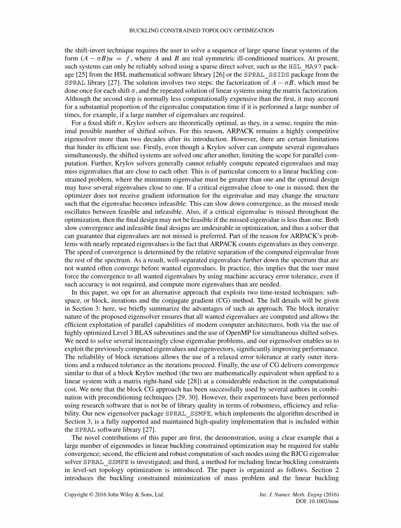
A simple example is used to illustrate the advantage of including more modes in a bucklingconstrained optimization problem. A 2D simply supported beam, subject to compressive load, isreinforced with vertical springs, as shown in Figure 1a. The beam is discretized using 60 beam ele-ments, which have two nodes and three degrees of freedom (dof) per node (two translations and
Figure 1. Beam buckling example: (a) Overview and (b) first two buckling modes.
Copyright © 2016 John Wiley & Sons, Ltd. Int. J. Numer. Meth. Engng (2016)DOI: 10.1002/nme
BUCKLING CONSTRAINED TOPOLOGY OPTIMIZATION
0.0
0.2
0.4
0.6
0.8
1.0
1.2
0.5
1.0
1.5
2.0
2.5
3.0
3.5
0 25 50 75
Loa
d fa
ctor
Obj
ecti
ve v
alue
Iteration
Objective Mode 1 Mode 2
1
2
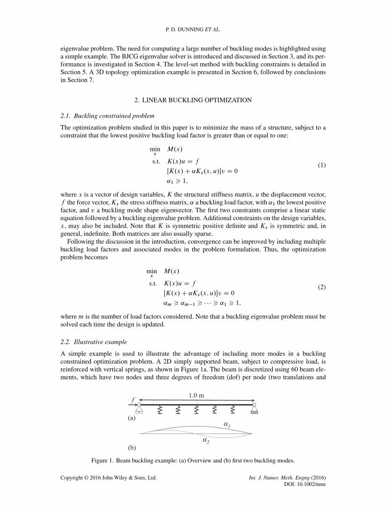
Figure 2. Convergence history using only the first buckling mode.
Figure 3. Optimal spring stiffness values for the beam reinforcement problem using a single mode with (a)no tracking and (b) tracking.
a rotation). The axial stiffness is modelled as a simple bar, and the bending stiffness is modelled asan Euler–Bernoulli beam [15]. The beam has a circular cross section with a diameter of 0.1 m andYoung’s modulus of 103. A spring is attached to each free node of the discretized beam.
The optimization problem is of the form (2); the stiffness values of the reinforcing springs are thedesign variables x, and their sum is the objective function M.x/. Note that for this simple example,u andKs do not depend on the design variables, as the beam is loaded in pure compression, and thesprings do not affect axial stiffness. The compressive force, f , is set to six times the Euler bucklingload of the unreinforced beam. The optimization problem is solved using the sequential quadraticprogramming method [31, 32] implemented in the package NLopt [33].
The beam reinforcement problem is first solved using a single mode (m D 1), and derivatives ofthe lowest positive eigenvalue with respect to the design variables are passed to the optimizer. Theload factors associated with the lowest two buckling modes are tracked during optimization usingan eigenvector orthogonality correlation method [34]. This procedure uses dot products betweenthe current and previous eigenvectors to match eigenvalues with the correct modes. The first twobuckling modes of the unreinforced beam are shown in Figure 1b. The convergence history of theobjective function and load factors are shown in Figure 2 and the solution is shown in Figure 3a.During the first 20 iterations, there is a switching of the critical mode every two or thre iterations,which severely slows down convergence. This is because only the derivatives of the current lowestload factor are computed at each iteration, and design changes that increase the first load factoroften decrease the second, although the change in the second load factor is two orders of magnitudesmaller. Despite the switching, the optimizer eventually increases both load factors, and a convergedfeasible design is obtained in 66 iterations.
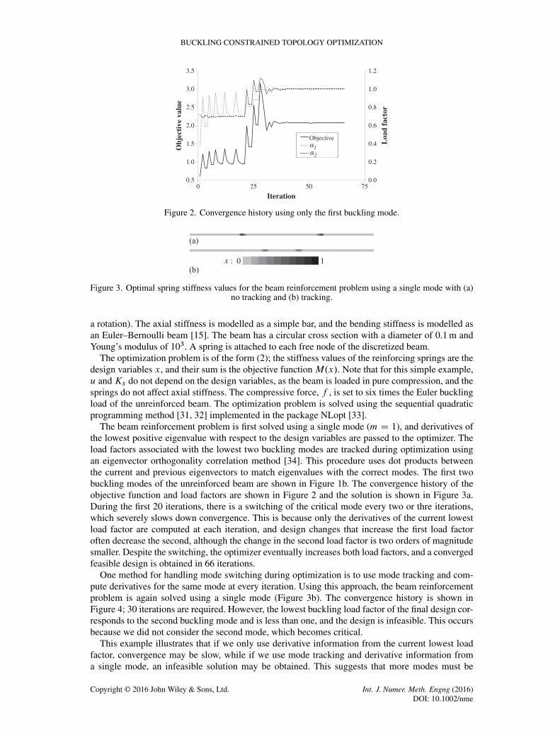
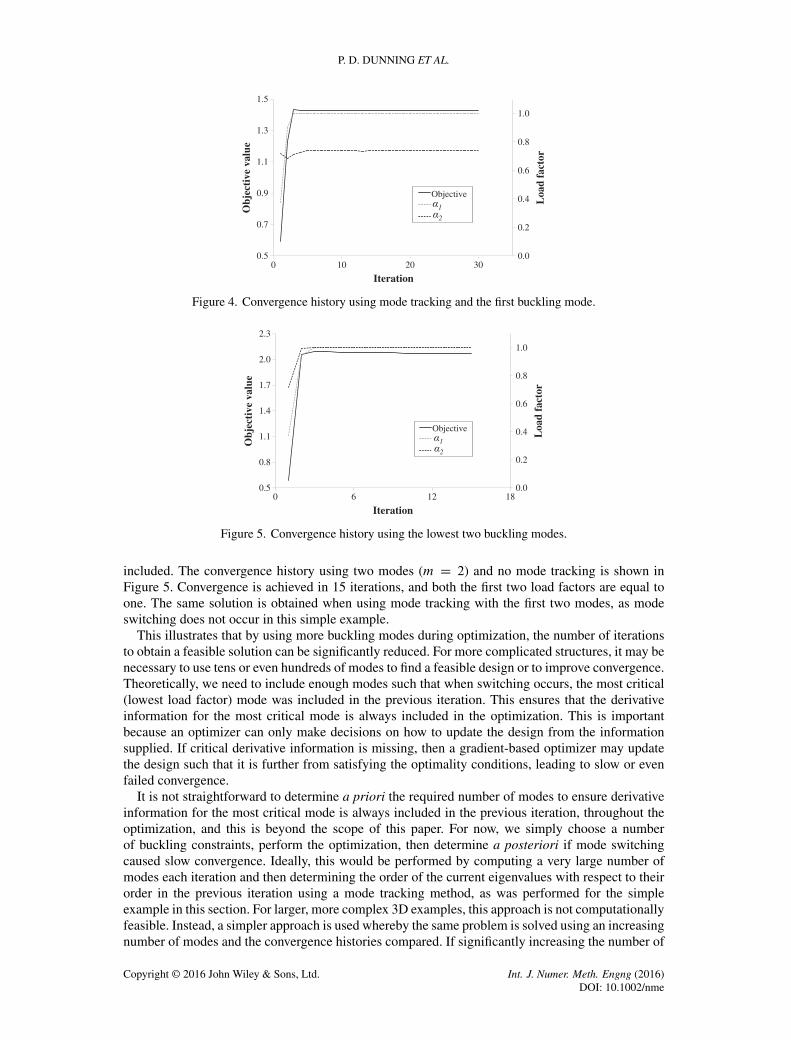
One method for handling mode switching during optimization is to use mode tracking and com-pute derivatives for the same mode at every iteration. Using this approach, the beam reinforcementproblem is again solved using a single mode (Figure 3b). The convergence history is shown inFigure 4; 30 iterations are required. However, the lowest buckling load factor of the final design cor-responds to the second buckling mode and is less than one, and the design is infeasible. This occursbecause we did not consider the second mode, which becomes critical.
This example illustrates that if we only use derivative information from the current lowest loadfactor, convergence may be slow, while if we use mode tracking and derivative information froma single mode, an infeasible solution may be obtained. This suggests that more modes must be
Copyright © 2016 John Wiley & Sons, Ltd. Int. J. Numer. Meth. Engng (2016)DOI: 10.1002/nme
P. D. DUNNING ET AL.
0.0
0.2
0.4
0.6
0.8
1.0
0.5
0.7
0.9
1.1
1.3
1.5
0 10 20 30
Loa
d fa
ctor
Obj
ecti
ve v
alue
Iteration
Objective Mode 1 Mode 2
1
2
Figure 4. Convergence history using mode tracking and the first buckling mode.
0.0
0.2
0.4
0.6
0.8
1.0
0.5
0.8
1.1
1.4
1.7
2.0
2.3
0 6 12 18
Loa
d fa
ctor
Obj
ecti
ve v
alue
Iteration
Objective Mode 1 Mode 2
1
2
Figure 5. Convergence history using the lowest two buckling modes.
included. The convergence history using two modes (m D 2) and no mode tracking is shown inFigure 5. Convergence is achieved in 15 iterations, and both the first two load factors are equal toone. The same solution is obtained when using mode tracking with the first two modes, as modeswitching does not occur in this simple example.
This illustrates that by using more buckling modes during optimization, the number of iterationsto obtain a feasible solution can be significantly reduced. For more complicated structures, it may benecessary to use tens or even hundreds of modes to find a feasible design or to improve convergence.Theoretically, we need to include enough modes such that when switching occurs, the most critical(lowest load factor) mode was included in the previous iteration. This ensures that the derivativeinformation for the most critical mode is always included in the optimization. This is importantbecause an optimizer can only make decisions on how to update the design from the informationsupplied. If critical derivative information is missing, then a gradient-based optimizer may updatethe design such that it is further from satisfying the optimality conditions, leading to slow or evenfailed convergence.
It is not straightforward to determine a priori the required number of modes to ensure derivativeinformation for the most critical mode is always included in the previous iteration, throughout theoptimization, and this is beyond the scope of this paper. For now, we simply choose a numberof buckling constraints, perform the optimization, then determine a posteriori if mode switchingcaused slow convergence. Ideally, this would be performed by computing a very large number ofmodes each iteration and then determining the order of the current eigenvalues with respect to theirorder in the previous iteration using a mode tracking method, as was performed for the simpleexample in this section. For larger, more complex 3D examples, this approach is not computationallyfeasible. Instead, a simpler approach is used whereby the same problem is solved using an increasingnumber of modes and the convergence histories compared. If significantly increasing the number of
Copyright © 2016 John Wiley & Sons, Ltd. Int. J. Numer. Meth. Engng (2016)DOI: 10.1002/nme
BUCKLING CONSTRAINED TOPOLOGY OPTIMIZATION
modes (such as doubling) does not reduce the number and magnitude of observed oscillations in theconvergence of the lowest buckling load factor, then it is reasonable to assume that enough modesare included to avoid convergence issues resulting from mode switching.
3. SOLVING THE GENERALIZED EIGENVALUE PROBLEM
As we have already observed, at the heart of the buckling constrained optimization problem liesa generalized eigenvalue problem that must be solved each time the design is updated. Moreover,a large number of buckling modes may be required to reduce oscillations during convergence andobtain feasible designs. In Section 3.1, we introduce the BJCG for solving a generalized eigenvalueproblem and then, in Section 3.2 , we discuss how this algorithm may be combined with shift-invertto efficiently and robustly solve the buckling eigenvalue problem.
3.1. Block Jacobi conjugate gradient algorithm
We start with the problem of computing m extreme (leftmost and/or rightmost) eigenvalues and thecorresponding eigenvectors of the generalized eigenvalue problem
ABv D �v; (3)
where A and B are real sparse symmetric n � n matrices with B positive definite and m� n. Themain features of the BJCG algorithm are its high computational intensity and inherent parallelism:the bulk of the computation is taken by dense matrix–matrix products and the simultaneous compu-tation of sparse matrix-vector products Avi and Bvi for a set of vectors vi . These features facilitateefficient exploitation of highly optimized matrix–matrix multiplication subroutines from the BLASlibrary and modern multicore computer architectures. The BJCG algorithm is based on the blockconjugate gradient method of [35–37] and is implemented as the software package SPRAL_SSMFE,which is available within the SPRAL mathematical software library [27].
In what follows, Œu1 � � � uk� denotes the matrix with columns u1; : : : ; uk , and for U DŒu1 � � � uk� and W D Œw1 � � � wl �; we denote ŒU W � D Œu1 � � � uk w1 � � � wl �. Alongsidethe standard notation .u;w/ for the Euclidean scalar product of two vectors u and w, we alsouse the following ‘energy scalar product’ and ‘energy norm’ notation: .u;w/H D .Hu;w/ andkuk2H D .Hu; u/, where H is positive definite or semi-definite. If .u; w/H D 0, then we say thatu and w are H -orthogonal, and if kukH D 1, then we say that u is H -normalized.
The BJCG algorithm for (3) essentially performs simultaneous optimization (minimizationor maximization or both depending on which eigenvalues are of interest) of the Rayleighquotient functional
�.u/ D.BABv; v/
.Bv; v/D.ABv; v/B
kvkB(4)
on sets of B-orthogonal vectors by a block version of the CG method. Focusing for simplicity onthe minimization case, we observe that the CG method minimizes a functional .u/ by iteratingtwo vectors: the current approximation vi to the minimum point v� D arg min .v/ and the currentsearch direction ui along which the next approximation viC1 is sought in the following manner:
viC1 D vi � �iui ; (5)
uiC1 D r �viC1
�C �iu
i : (6)
Step (5) finds the minimum of .v/ in the direction set by ui , that is, �i D arg min i .�/, where i .�/ D .v
i��ui /. Step (6), referred to as the conjugation of search directions, computes the newsearch direction uiC1 based on the gradient of .v/ at v D viC1 and the previous search direction ui
(not present at the first iteration). The role of the scalar parameter �i is to make the search directioncloser to the ideal one, the error direction vi � v�, which would result in an immediate convergenceon the next iteration. In the case of a quadratic functional .v/ D .Av; v/�2.f; v/with a symmetric
Copyright © 2016 John Wiley & Sons, Ltd. Int. J. Numer. Meth. Engng (2016)DOI: 10.1002/nme
P. D. DUNNING ET AL.
positive definite A, the minimum of which solves the linear system Av D f , it is possible to choose�i in such a way that all vi are optimal, that is, each .vi / is the smallest possible value achievableby iterations (5)–(6). In the non-quadratic case, such optimality is generally not achievable. In [35],various suggestions for �i have been studied thoroughly to arrive at the conclusion that most of themare asymptotically equivalent and make the value .viC2/ ‘nearly’ the smallest possible for a givenviC1 and ui . It should be noted that the value of �i that makes .viC2/ the smallest possible can becomputed by finding the minimum of .v/ among all linear combinations of viC1, r .viC1/ andui [30, 38]; however, this locally optimal version of CG is numerically unstable [37].
When computing several eigenpairs by simultaneous optimization of the Rayleigh quotient (4), itis necessary to maintain the B-orthogonality of approximate eigenvectors vij lest they converge tothe same eigenvector corresponding to an extreme eigenvalue. One way to achieve this, which hasan additional benefit of improved convergence, is to employ the Rayleigh–Ritz procedure. Given aset of vectors ´1; : : : ; ´k , k < n, this procedure solves the generalized eigenvalue problem
ZTBABZ Ov D O�ZTBZ Ov; (7)
where Z D Œ´1 � � � ´k�. The vectors Qvj D Z Ovj , where Ovj are the eigenvectors of (7), are calledRitz vectors, and the corresponding eigenvalues O�j D �. Qvj / are called Ritz values. In what fol-lows, we refer to ´i as the basis vectors of the Rayleigh–Ritz procedure, and we use the following‘function call’ notation for this procedure: for a given Z D Œ´1 � � � ´k�, Y D RayleighRitz.Z/is the matrix whose columns are B-normalized Ritz vectors. The Ritz vectors are B-orthogonalby construction, and if there exists a linear combination of the basis vectors that approximates aneigenvector of (3), then there exists a Ritz vector that approximates this eigenvector to a compa-rable accuracy [39]. The aforementioned two ingredients, CG and the Rayleigh–Ritz procedure,are blended in the BJCG algorithm in the following way. The line search step (5) is replaced bythe Rayleigh–Ritz procedure that uses all approximate eigenvectors vij and all search directionsuij as the basis vectors, and a matrix analogue of (6) is used for conjugation, which after simplemanipulations yields the iterative scheme�
V iC1 W iC1�D RayleighRitz
�V i ; U i
�; (8)
U iC1 D RiC1 CW iC1Si : (9)
In (8), the columns of V iC1 approximate the eigenvectors of interest, that is, if we are computingml > 0 leftmost and mr > 0 rightmost eigenvalues and corresponding eigenvectors, then them D ml Cmr columns of V iC1 correspond to the ml leftmost and mr rightmost Ritz values. Therest of the Ritz vectors are the columns of W iC1 and are used as the previous search directions forconjugation (this is shown by Ovtchinnikov [36] to be mathematically equivalent to using U i in (9)but simplifies the calculation of the optimal conjugation matrix Si ). In (9), RiC1 D Œr iC11 � � � r iC1m �,where r iC1j D ABviC1j � �.viC1j /viC1j are the residual vectors for viC1j , which are collinear to thegradients of � in B-scalar product. For the elements �pq of the matrix Si , the following formulaewere derived in [36] that ensure the asymptotic local optimality of the new search directions:
�pq D �
�r iC1q ; BABwiC1p � �
�viC1q
�BwiC1p
���wiC1p
�� �
�viC1q
� : (10)
While the columns of V i are B-orthonormal, some of the columns of U i may be nearly linearlydependent on the rest of the basis vectors. Such vectors are removed from the set of basis vectors toavoid numerical instability caused by the ill-conditioned matrix ZTBZ in (7). The number of Ritzvectors then reduces accordingly, and Si has less rows than columns.
We observe that the most costly computational steps of the described algorithm in terms of thenumber of arithmetic operations are as follows:
Copyright © 2016 John Wiley & Sons, Ltd. Int. J. Numer. Meth. Engng (2016)DOI: 10.1002/nme
BUCKLING CONSTRAINED TOPOLOGY OPTIMIZATION
(1) The computation of sparse-by-dense matrix products V iBDBVi ,AV iB , U iBDBU
i andAU iB .(2) The computation of dense matrix–matrix products ZTBZA and ZTZB with Z D ŒV i U i �,
ZA D AZB and ZB D BZ.(3) The computation of V iC1 and W iC1 from the eigenvectors of (7) by dense matrix–matrix
products.(4) The computation of sparse-by-dense matrix products W iC1
B D BW iC1 and AW iC1B .
(5) The computation of a dense matrix–matrix product W iC1Si .
(The A-images and B-images of V iC1 and W iC1 can be alternatively computed from those of V i
and U i , which reduces the number of multiplications by A and B threefold at the cost of extrastorage [30].) The computational cost of the rest of the algorithm is negligible ifm� n. We observethat steps 2, 3 and 5 require dense matrix–matrix multiplications that can be efficiently performedby highly optimized BLAS subroutines, for exmples, those provided by Intel MKL library, whichalso has highly optimized subroutines for sparse-by-dense matrix multiplications performed on steps1 and 4.
3.2. Application of block Jacobi conjugate gradient to the buckling eigenvalue problem
In this section, we show how we use the BJCG algorithm to compute buckling modes, that is,eigenvalues ˛i and eigenvectors vi of the generalized eigenvalue problem
.K C ˛Ks/v D 0; (11)
where K and Ks are n � n real sparse symmetric matrices, K is positive definite and Ks is indef-inite. The eigenvalues of interest lie in the vicinity of 1, notably: any eigenvalues ˛i that lie in theinterval .0; 1� are required and several eigenvalues ˛i > 1 that are closest to 1, together with the cor-responding eigenvectors. As in the previous section, m denotes the number of wanted eigenvalues;all eigenvalues are assumed to be enumerated in ascending order.
We observe immediately that (11) can be rewritten as the generalized eigenvalue problem
Ksv D ˇKv; (12)
where ˇ D �˛�1. The BJCG algorithm can be applied to this problem, but convergence maybe very slow, as can be seen from the following simplified illustration that extends the informaldiscussion of the convergence of block CG given in [30].‡ Suppose that we start the BJCG iterationswith the initial vectors v0j D vj , j D 2; : : : ; m and with v01 close to v1 and K-orthogonal tov2; : : : ; vm. It can be shown that the BJCG iterations then reduce to single-vector CG iterations(5)–(6) for computing the zero eigenvalue of A1 D Ks � ˇ1K, performed in the subspace that isA1-orthogonal to v2; : : : ; vm. Using the comparative convergence analysis techniques developed in[35], it can be shown that these iterations are asymptotically close to the CG iterations for the systemA1v1 D 0 in that subspace. For the error vi1�v1, we have kvi1�v1k
2A1D .A1.v
i1�v1/; v
i1�v1/ D
.A1vi1; v
i1/ D .ˇ
i1�ˇ1/.Kv
i1; v
i1/, where ˇi1 D .Ksv
i1; v
i1/=.Kv
i1; v
i1/. Therefore, from the standard
CG convergence estimate for kvi1�v1kA1 , we obtain, after dropping asymptotically small terms, anestimate similar to that conjectured in [30]:
ˇi1 � ˇ1 .�p
�1 � 1p�1 C 1
�2i �ˇ01 � ˇ1
�; (13)
where �1 is the ratio of the n-th to .mC1/-th eigenvalue of the matrixKs�ˇ1K (for BJCG, a similarestimate without square roots is proved in [36]). Because ˇ1 � �1 and K is the discretization ofa partial differential operator, the n-th (i.e. the largest) eigenvalue of Ks � ˇ1K is very large, andhence the ratio in question is very small, leading to unacceptably slow convergence.
‡ Rigorous convergence analysis of CG for eigenvalue computation is very difficult, and virtually all available resultsmerely state that the convergence of CG is at least as fast as that of steepest descent, whereas in reality the convergenceof CG is much faster and is more adequately portrayed by a conjectured estimate of [30] and those of this section.
Copyright © 2016 John Wiley & Sons, Ltd. Int. J. Numer. Meth. Engng (2016)DOI: 10.1002/nme
P. D. DUNNING ET AL.
To achieve good convergence, we resort to the shift-invert technique. We pick a value ˛0 in theeigenvalue region of interest and rewrite (11) as
.K C ˛0Ks/�1Kv D �v; (14)
where
� D˛
˛ � ˛0: (15)
We observe that (14) is of the form (3) with
A D .K C ˛0Ks/�1; B D K (16)
and hence can be solved by the BJCG algorithm.To illustrate how the transformation from (11) to (14) improves the convergence, let us assume for
simplicity that ˛0 D .˛mC˛mC1/=2. Then the leftmost eigenvalue of (14) is �1 D ˛m=.˛m�˛0/ <0, the rightmost is �n D ˛mC1=.˛mC1 � ˛0/ > 0 and the number of negative �i is m, that is,�mC1 > 0. Just as with (12), the convergence rate for �1 is determined by the ratio of the n-th tomC 1-th eigenvalue of the matrix .K C ˛0Ks/�1K � �1I , where I is the identity matrix, that is,by the ratio
�1 D�n � �1
�mC1 � �16 ��n � �1
�1D 1 �
�n
�1D 1 �
˛mC1
˛m
˛m � ˛0
˛mC1 � ˛0D 1C
˛mC1
˛m� 2:
The substitution of this �1 into (13) with �1 and its approximations � i1 in place of ˇ1 and ˇi1 yields
� i1 � �1 . p
2 � 1p2C 1
!2i ��01 � �1
�� 0:03i
��01 � �1
�:
Thus, just two iterations reduce the eigenvalue error by three orders of magnitude.When dealing with eigenvalues on both ends of the spectrum simultaneously, it is convenient to
use positive indices for the eigenvalues on the left margin: �1 6 �2 6 � � � , and negative for those onthe right margin: ��1 > ��2 > � � � (i.e. ��j D �n�jC1). Let ml and mr be the number of wantedeigenvalues of (11) to the left and right of ˛0, respectively. The same kind of reasoning as we usedfor deriving (13) suggests the following estimate for further eigenvalues of (14):
� ij � �j .�p
�j � 1p�j C 1
�2i ��0j � �j
�; (17)
where
�j D��mr�1 � �j
�mlC1 � �j; ��j D
��j � �mlC1
��j � ��mr�1; j > 0: (18)
The estimate (17)–(18) has practical implications, in particular, the following one.
Remark 1Because the density of the spectrum increases towards � D 1, for a large mr , the value ��mr ���mr�1 may be very small. Therefore, to avoid very slow convergence to ��j that are close to��mr�1, the block size m of BJCG should be set to a value that is larger than the actual number ofwanted eigenvalues. The effect of the increased block size can be seen from (18) where, if the blocksize is increased by k > 0, one should replace ��mr�1 with ��mr�k�1, which reduces both �j and��j . Note that the additional eigenvalues and eigenvectors need not be accurately computed. that is,the BJCG iterations should be stopped as soon as �1; : : : ; �ml and ��1; : : : ; ��mr and correspondingeigenvectors converge to required accuracy.
We note that the spectral transformation (15) maps the eigenvalues as follows. The eigenvaluesin the interval .0; ˛0/ correspond to all negative �i . The eigenvalues of interest to the right of ˛0correspond to the rightmost �i . The rest of the spectrum of (11) corresponds to a huge cluster of
Copyright © 2016 John Wiley & Sons, Ltd. Int. J. Numer. Meth. Engng (2016)DOI: 10.1002/nme
BUCKLING CONSTRAINED TOPOLOGY OPTIMIZATION
�i around � D 1. When using BJCG for solving (14), it is very important to set the number of wantedleftmost eigenvaluesml exactly to the number of negative �i . Settingml to a larger value will resultin a large number of iterations, as BJCG will try to compute an eigenvalue in the cluster at � D 1.For this reason, using an LDLT factorization for solving the shifted system .KC ˛0Ks/x D y (thisis needed for computing the product Ay (16) in BJCG) is strongly recommended (e.g. the directsolvers HSL_MA97 [25] or SPRAL_SSIDS [27] may be used). Recall that an LDLT factorizationof the matrix K C ˛0Ks consists in finding a unit lower triangular matrix L, a block-diagonalmatrix D with 1 � 1 and 2 � 2 blocks on the main diagonal and a permutation matrix P such thatP T .K C ˛0Ks/P D LDLT . By the inertia theorem, the number of eigenvalues to the left andright of the shift ˛0 is equal to the number of negative and positive eigenvalues of D, which allowsquick computation of the number of eigenvalues to each side of the shift after. Knowing the numberof eigenvalues to the left of ˛0 also helps avoid recomputation of the already computed bucklingmodes after a new shift.
Remark 2If the number of wanted buckling modes is very large, or the number of eigenvalues on each sideof the shift ˛0 are disproportional, multiple shifts should be considered. Note that for each choiceof shift ˛0, a factorization of K C ˛0Ks is required. Once the factorization has been performed, thefactors may be used repeatedly for solving any number of systems.
The decision on whether to use more than one shift can be made on the basis of a ‘trial run’,whereby a portion (e.g. a quarter) of the wanted buckling modes is computed, and the time takenby BJCG is extrapolated and compared with the factorization time. This can also be used to selecta better shift, based on the number of eigenvalues on each side of the initial shift. If no new shift isdeemed to be necessary, the remaining buckling modes can be computed by BJCG in the subspaceK-orthogonal to the computed eigenvectors.
In this paper, the shift-invert solves are performed using a sparse direct linear solver. Alterna-tively, an iterative method could be used. Such methods have the potential advantage of requiringmuch less memory and so can be used to solve very large linear systems of equations. However, ingeneral, to achieve an acceptable rate of convergence, a preconditioner is required; unfortunately,designing an efficient preconditioner is highly problem-dependent, and we are not aware of such pre-conditioners for linear buckling problems. Note that if we were able to obtain such a preconditioner,it would be unnecessary to solve the shifted system using a preconditioned iterative method becauseSPRAL_SSMFE can employ preconditioning directly, a feature not shared by Krylov solvers, byessentially applying BJCG iterations to the problem T .K C ˛Ks/v D 0, where T is the precondi-tioner, without first converting to the shifted system (14). The design of an efficient preconditioneris beyond the scope of this paper and is a topic for future research.
3.3. Application to topology optimization
As we have seen in Section 2, topology optimization algorithms require the solution of a sequenceof buckling eigenvalue problems. As the outer (optimization) iterations progress, these problemsbecome ever closer to each other, which suggests using data from the previous outer iteration for theacceleration of BJCG convergence on the next outer iteration.
An obvious approach is to use the buckling modes from the previous outer iteration as the initialapproximations v01 ; : : : ; v
0m for BJCG. Another option is to use the approximate eigenvalues com-
puted on the previous outer iteration and the estimate (17)–(18) to select ˛0. Note that �j is anincreasing function of �j , and ��j is a decreasing function of ��j . Hence, their maxima are �mland ��mr , respectively. A good choice for ˛0 therefore should make the maximum of these twovalues the minimal possible. There is an obstacle however: �mlC1 may be difficult to compute. Tobypass this, assume that any negative ˛i is sufficiently far away from zero, so that �mlC1 � 1.Let Q̨j , j D 1;m, be the eigenvalues of (11) computed on the previous outer iteration. Assuming�mlC1 D 1, we obtain from (15) and (18) via elementary calculation
�ml D˛mC1 � Q̨1
˛mC1 � ˛0; ��mr D
˛mC1 � ˛0
˛mC1 � Q̨m: (19)
Copyright © 2016 John Wiley & Sons, Ltd. Int. J. Numer. Meth. Engng (2016)DOI: 10.1002/nme
P. D. DUNNING ET AL.
We observe that �ml is an increasing function of ˛0 and ��mr is a decreasing one. Hence, themaximum of the two is minimal when �ml D ��mr , which is attained at
˛0 D ˛mC1 �p.˛mC1 � Q̨1/.˛mC1 � Q̨m/: (20)
In practice, ˛mC1 is replaced by an approximation. We also note that if the block size of BJCG isincreased by k > 0 to improve convergence (cf. Remark 1), then in (20), ˛mC1 should be replacedby an approximation to ˛mCkC1, or simply by q Q̨m, where q > 1 (e.g. q D 1:1, which roughlycorresponds to k D m=10), which yields
˛0 D q Q̨m �p.q Q̨m � Q̨1/.q � 1/ Q̨m: (21)
This paper assumes a linear relationship between loads, deflections and stresses, and that deflec-tions are small. These assumptions allow the use of a linear buckling analysis, which is an efficientmethod for estimating the critical buckling load factor and is useful in engineering design. However,linear buckling analysis often overestimates the critical load when imperfections and non-linearitiesare accounted for. When these factors are significant, non-linear buckling analysis can be performed.For topology optimization of geometrically non-linear structures, Lindgaard and Dahl [12] suggestusing the arc length method for geometrically non-linear analysis until an instability is detected. Abuckling eigenvalue analysis is then performed for the structure in the configuration one step beforethe instability occurs. Therefore, when using this approach, it may be possible to use the BJCGmethod to reduce the computational cost of the eigenvalue analysis when performing optimizationwith non-linear buckling constraints.
4. PERFORMANCE OF THE EIGENVALUE SOLVER
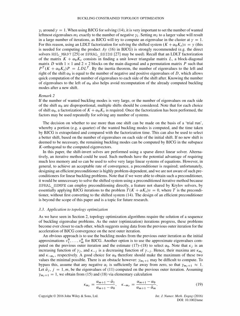
In this section, we use two linear buckling problems to benchmark the performance of our BJCGeigenvalue solver SPRAL_SSMFE and to highlight its potential for the efficient computation of alarge number of buckling eigenmodes during optimization. The two examples are rectangular bladestiffened panels, simply supported and loaded in compression along their short edges (Figure 6).Both panels are 1 m � 0.5 m and have evenly spaced blade stiffeners. The depth of the stiffenersis 25 mm and 30 mm, respectively. The material properties are Young’s modulus of 70 GPa andPoisson’s ratio of 0.32. The panels are discretized using three-node shell elements, with six dof pernode. The thickness of the shells are 4 mm and 3 mm, respectively. Different levels of discretizationare used to test the scalability of SPRAL_SSMFE.
The tests are performed on a 16-core Intel(R) Xeon(R) E5-2687W CPU, and the GNUgfortran compiler with flags -O3 -fopenmp are used. The factorization of the shifted matricesKC˛0Ks and subsequent solves is performed by HSL_MA97 [26] run in parallel mode. The shiftedsolves are performed by the solver subroutines from HSL_MA97 called in an OpenMP parallel doloop each using one MKL thread.
Unless specified explicitly, a shift of ˛0 D 1 and an eigenvector error tolerance of 10�4 is usedin the reported tests. The BJCG block size for computing k modes is set to k Cmax.10; k=10/. Allreported timings are measured using the function clock_gettime and are in seconds.
Figure 6. Buckling examples: (a) Panel 1 and (b) Panel 2.
Copyright © 2016 John Wiley & Sons, Ltd. Int. J. Numer. Meth. Engng (2016)DOI: 10.1002/nme
BUCKLING CONSTRAINED TOPOLOGY OPTIMIZATION
Table I. Timings for Panel 1 using different discretizations.
Problem size Time per Factorization(dof) Solve time 103 dof time
8902 0.7 0.083 0.117576 1.4 0.079 0.237625 3.1 0.081 0.374383 6.7 0.090 0.5144823 12.1 0.084 1.0224522 19.6 0.087 1.6394962 36.3 0.092 2.9577643 54.7 0.095 4.6728142 61.0 0.084 5.1908065 83.1 0.092 7.4
Table II. Performance data for different numbers of modes for Panel 1 with577 643 dof.
Shifted Time per Shifted solvesModes Solve time Iterations solves mode per mode
20 22.5 16 443 1.13 2240 29.7 17 712 0.74 1860 38.1 17 981 0.64 1680 48.9 14 1145 0.61 14100 54.7 16 1394 0.55 14
Table I displays SPRAL_SSMFE solve and HSL_MA97 factorization timings for different lev-els of discretization for Panel 1, where 100 buckling eigenmodes are computed. The third columnpresents the solve times divided by the dof in thousands. We observe a nearly linear scaling of thesolve times with the problem size. Similar results are obtained for Panel 2. This shows the poten-tial of SPRAL_SSMFE to efficiently compute buckling eigenvalues and eigenvectors for large-scaleoptimization problems.
Table II shows performance data for Panel 1 (using the 577 643 dof discretization) for differentnumbers of buckling modes. The block sizem is set to the number of modes plus 10. We observe thatthe number of BJCG iterations remains practically unchanged as the number of modes increases,thanks to the increase in the block size, which improves the convergence to leftmost modes (see [36]for the convergence analysis of BJCG). The last two columns show that the time per mode and thenumber of shifted solves per mode decreases for larger numbers of modes. This is a promising resultwhen we consider that a large number of buckling eigenmodes may be required during optimization,as discussed in Section 2.2.
Table III shows the results of using different shifts ˛0 for computing 100 modes for Panel 1 (usingthe 577 643 dof discretization). We observe that the minimal number of BJCG iterations and shiftedsolves is attained at ˛0 D 20, which is very close to the optimal shift value of 20.3 predicted by (21)with q D 1:1.
Table IV shows analogous results for Panel 2 (using a 539 291 dof discretization). In this case,the best shift (in terms of the iteration number) is ˛0 D 11, which is further from the theoreticallyoptimal ˛0 D 14:4. This is because of the rapidly increasing density of the spectrum to the right from˛0, which makes the linear extrapolation ˛mCkC1 � .1C .k C 1/=m/ Q̨m used in (21) inaccurate.
Remark 3To highlight potential problems with employing ARPACK in topology optimization, we usedARPACK to compute the 100 leftmost eigenvalues of Panel 2 (539 291 dof) with ˛0 D 9 andmaximal accuracy, that is, the ARPACK tolerance was set to zero. The leftmost eigenvalue ˛1 D�1:1434995674 is closer to ˛0 than ˛100 D �18:472317385, so we expected that ARPACK wouldcompute all the wanted 42 eigenpairs that lie to the left of ˛0. However, 22 were missing, that is,ARPACK computed ˛23 to ˛122 instead of the wanted ˛1 to ˛100.
Copyright © 2016 John Wiley & Sons, Ltd. Int. J. Numer. Meth. Engng (2016)DOI: 10.1002/nme
P. D. DUNNING ET AL.
Table III. Performance data for different shifts for Panel 1 with 577 643 dof.
Shift Eigenvalues Eigenvalues Shifted˛0 left of ˛0 right of ˛0 Solve time Iterations solves
1 0 100 54.7 16 13945 4 96 52.5 14 127710 10 90 50.7 13 117215 30 70 44.3 11 105519 49 51 43.1 11 104020 55 45 41.3 11 102021 65 35 40.4 13 102721.3 66 34 40.0 13 104222 68 32 40.9 14 106225 88 12 49.2 17 1233
Table IV. Performance data for different shifts for Panel 2 with 539 291 dof.
Shift Eigenvalues Eigenvalues Shifted˛0 left of ˛0 right of ˛0 Solve time Iterations solves
1 0 100 47.1 16 12752 3 97 46.0 16 12563 8 92 46.4 15 12114 15 85 43.0 15 11695 20 80 46.5 16 11686 23 77 43.5 14 11397 32 68 42.3 14 11258 37 63 39.4 12 10959 42 58 38.3 12 108010 49 51 38.5 11 109711 56 44 39.7 10 109212 63 37 40.3 11 113213 67 33 40.5 11 115714 73 27 43.7 14 119614.4 76 24 46.9 14 1233
Table V. Times using a single shift and two shifts for 200 modes for Panels1 and 2.
Panel 1 Panel 2
Shifts Factorization Solve Total Factorization Solve Total
1 4.6 143.9 148.5 4.2 109.7 113.92 9.2 114.9 124.1 8.4 98.6 107.0
In Table V, we compare the computation of 200 modes using one shift ˛0 for the computation of100 modes and then the remaining 100 modes using a new shift ˛100 C 5 � .˛100 � ˛90/ � ˛150.For this example, we observe that when computing 200 modes, two shifts are preferable to a singleshift. However, the opposite is observed when a total of 100 modes are computed. Thus, the multipleshift strategy may provide additional efficiency gains during optimization when a large number ofbuckling modes is required.
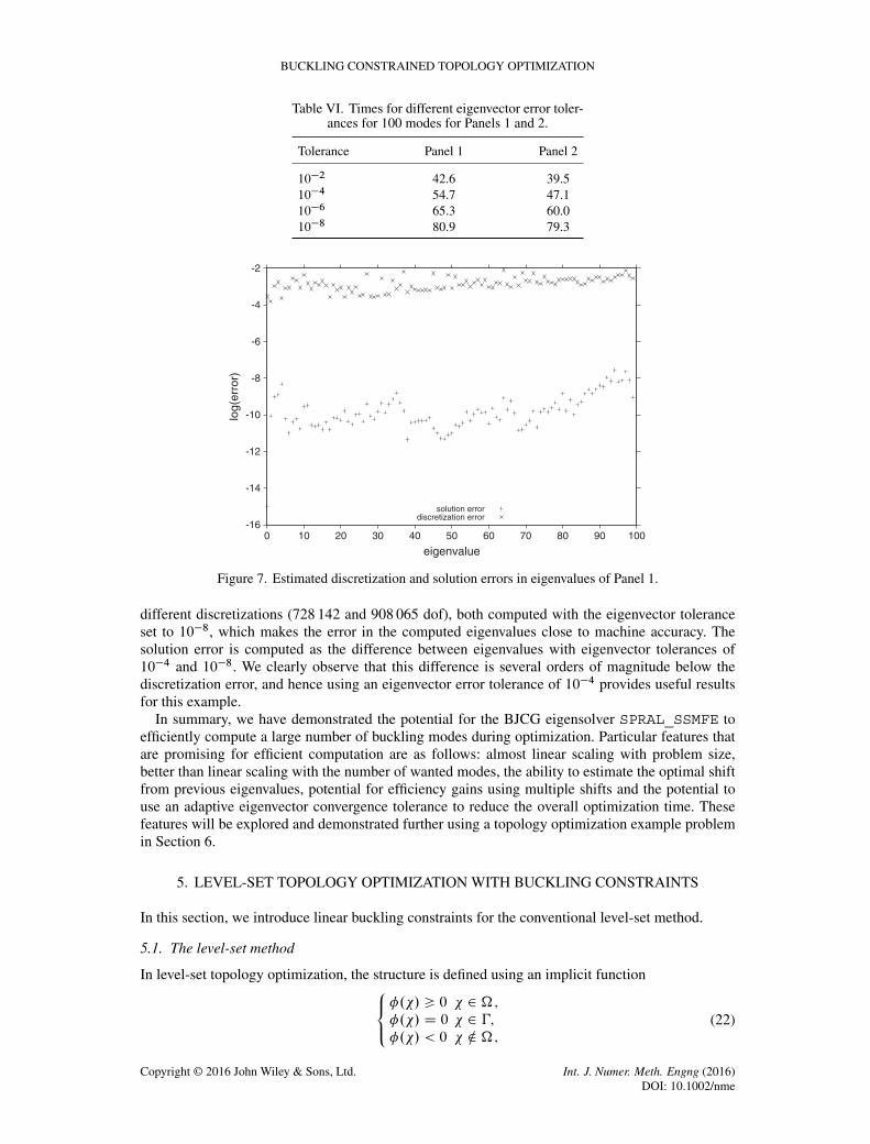
Table VI compares the solve times for 100 modes for Panels 1 and 2 for various eigenvector errortolerances. It takes approximately twice as long to compute eigenvectors with 10�8 accuracy aswith 10�2 accuracy. This suggests that using a relaxed tolerance at early outer iterations, when thecomputed modes are far from optimal, then a progressively smaller tolerance as the outer iterationsproceed is a potential strategy for reducing the overall optimization time.
Figure 7 provides a justification for the use of the eigenvector error tolerance of 10�4 in mosttests by comparing the estimated discretization and solution errors in eigenvalues of Panel 1 using728 142 dof. The discretization error is computed as the difference between the eigenvalues at two
Copyright © 2016 John Wiley & Sons, Ltd. Int. J. Numer. Meth. Engng (2016)DOI: 10.1002/nme
BUCKLING CONSTRAINED TOPOLOGY OPTIMIZATION
Table VI. Times for different eigenvector error toler-ances for 100 modes for Panels 1 and 2.
Tolerance Panel 1 Panel 2
10�2 42.6 39.510�4 54.7 47.110�6 65.3 60.010�8 80.9 79.3
-16
-14
-12
-10
-8
-6
-4
-2
0 10 20 30 40 50 60 70 80 90 100
log(
erro
r)
eigenvalue
solution errordiscretization error
Figure 7. Estimated discretization and solution errors in eigenvalues of Panel 1.
different discretizations (728 142 and 908 065 dof), both computed with the eigenvector toleranceset to 10�8, which makes the error in the computed eigenvalues close to machine accuracy. Thesolution error is computed as the difference between eigenvalues with eigenvector tolerances of10�4 and 10�8. We clearly observe that this difference is several orders of magnitude below thediscretization error, and hence using an eigenvector error tolerance of 10�4 provides useful resultsfor this example.
In summary, we have demonstrated the potential for the BJCG eigensolver SPRAL_SSMFE toefficiently compute a large number of buckling modes during optimization. Particular features thatare promising for efficient computation are as follows: almost linear scaling with problem size,better than linear scaling with the number of wanted modes, the ability to estimate the optimal shiftfrom previous eigenvalues, potential for efficiency gains using multiple shifts and the potential touse an adaptive eigenvector convergence tolerance to reduce the overall optimization time. Thesefeatures will be explored and demonstrated further using a topology optimization example problemin Section 6.
5. LEVEL-SET TOPOLOGY OPTIMIZATION WITH BUCKLING CONSTRAINTS
In this section, we introduce linear buckling constraints for the conventional level-set method.
5.1. The level-set method
In level-set topology optimization, the structure is defined using an implicit function8<:./ > 0 2 �;./ D 0 2 �;./ < 0 … �;
(22)
Copyright © 2016 John Wiley & Sons, Ltd. Int. J. Numer. Meth. Engng (2016)DOI: 10.1002/nme
P. D. DUNNING ET AL.
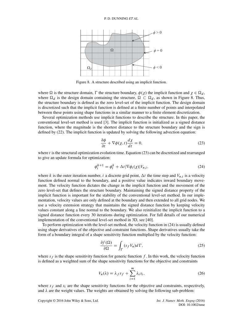
Figure 8. A structure described using an implicit function.
where � is the structure domain, � the structure boundary, ./ the implicit function and 2 �d ,where �d is the design domain containing the structure, � � �d , as shown in Figure 8. Thus,the structure boundary is defined as the zero level-set of the implicit function. The design domainis discretized such that the implicit function is defined at a finite number of points and interpolatedbetween these points using shape functions in a similar manner to a finite element discretization.
Several optimization methods use implicit functions to describe the structure. In this paper, theconventional level-set method is used [3]. The implicit function is initialized as a signed distancefunction, where the magnitude is the shortest distance to the structure boundary and the sign isdefined by (22). The implicit function is updated by solving the following advection equation:
@
@tCr.; t/
d
dtD 0; (23)
where t is the structural optimization evolution time. Equation (23) can be discretized and rearrangedto give an update formula for optimization:
kC1i D ki C t jri ./jVn;i ; (24)
where k is the outer iteration number, i a discrete grid point, t the time step and Vn;i is a velocityfunction defined normal to the boundary, and a positive value indicates inward boundary move-ment. The velocity function dictates the change in the implicit function and the movement of thezero level-set that defines the structure boundary. Maintaining the signed distance property of theimplicit function is important for the stability of the conventional level-set method. In our imple-mentation, velocity values are only defined at the boundary and then extended to all grid nodes. Weuse a velocity extension strategy that maintains the signed distance function by keeping velocityvalues constant along a line normal to the boundary. We also reinitialize the implicit function to asigned distance function every 30 iterations during optimization. For full details of our numericalimplementation of the conventional level-set method in 3D, see [40].
To perform optimization with the level-set method, the velocity function in (24) is usually definedusing shape derivatives of the objective and constraint functions. Shape derivatives usually take theform of a boundary integral of a shape sensitivity function multiplied by the velocity function:
@f .�/
@�D
Z�
.sf Vn/d�; (25)
where sf is the shape sensitivity function for generic function f . In this work, the velocity functionis defined as a weighted sum of the shape sensitivity functions for the objective and constraints
Vn.�/ D �f sf C
mXiD1
�isi ; (26)
where sf and si are the shape sensitivity functions for the objective and constraints, respectively,and � are the weight values. The weights are obtained by solving the following sub-problem:
Copyright © 2016 John Wiley & Sons, Ltd. Int. J. Numer. Meth. Engng (2016)DOI: 10.1002/nme
BUCKLING CONSTRAINED TOPOLOGY OPTIMIZATION
min� f .Vn.�//
s.t. gi .Vn.�// 6 Gi ; i D 1 : : : m�min 6 � 6 �max
(27)
where Gi is the target change for constraint function gi , set to maintain constraint feasibility, and f is an approximation for the change in f for a given velocity function, which is obtained byusing numerical integration to evaluate (25). Full details on this approach for handling constraintsin level-set-based optimization are given in [41].
5.2. Buckling constraints
An important aspect of structural optimization using the level-set method is the formulation ofthe structural stiffness and mass properties from the implicit function. Here, an efficient fixed gridapproach is used, where the background FE mesh remains fixed and the properties of elements cutby the boundary are approximated using a volume weighted approach:
NEi D �iE;
N�i D �i�;(28)
where E and � are the Young’s modulus and density of the structural material, the over bar denotesthe effective material properties for element i used to build the FE matrices and �i is the volume-fraction, defined as
�i DVol i
Vol i.1 � �min/C �min; (29)
where Vol i is the volume of element i that lies inside the structure, Vol i is the total volume of theelement and �min is a small positive value to avoid singular matrices, �min D 10
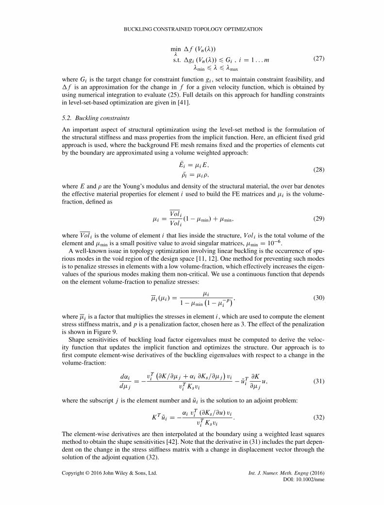
�6.A well-known issue in topology optimization involving linear buckling is the occurrence of spu-
rious modes in the void region of the design space [11, 12]. One method for preventing such modesis to penalize stresses in elements with a low volume-fraction, which effectively increases the eigen-values of the spurious modes making them non-critical. We use a continuous function that dependson the element volume-fraction to penalize stresses:
�i .�i / D�i
1 � �min�1 � �
�pi
� ; (30)
where �i is a factor that multiplies the stresses in element i , which are used to compute the elementstress stiffness matrix, and p is a penalization factor, chosen here as 3. The effect of the penalizationis shown in Figure 9.
Shape sensitivities of buckling load factor eigenvalues must be computed to derive the veloc-ity function that updates the implicit function and optimizes the structure. Our approach is tofirst compute element-wise derivatives of the buckling eigenvalues with respect to a change in thevolume-fraction:
d˛i
d�jD �
vTi�@K=@�j C ˛i @Ks=@�j
�vi
vTi Ksvi� QuTi
@K
@�ju; (31)
where the subscript j is the element number and Qui is the solution to an adjoint problem:
KT Qui D �˛i v
Ti .@Ks=@u/ vi
vTi Ksvi: (32)
The element-wise derivatives are then interpolated at the boundary using a weighted least squaresmethod to obtain the shape sensitivities [42]. Note that the derivative in (31) includes the part depen-dent on the change in the stress stiffness matrix with a change in displacement vector through thesolution of the adjoint equation (32).
Copyright © 2016 John Wiley & Sons, Ltd. Int. J. Numer. Meth. Engng (2016)DOI: 10.1002/nme
P. D. DUNNING ET AL.
Figure 9. Stress penalization factor.
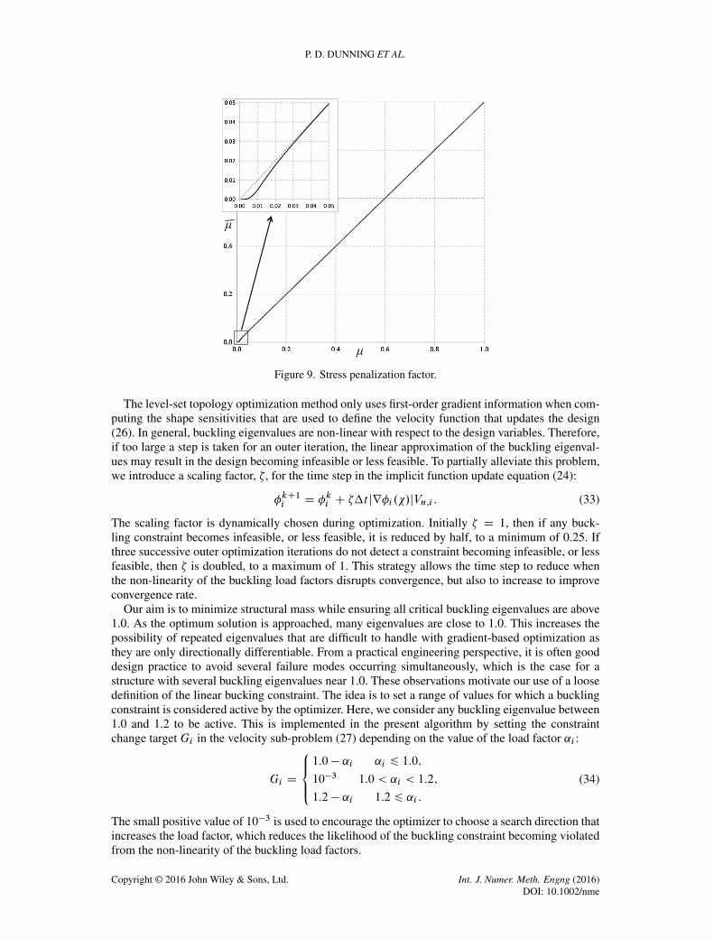
The level-set topology optimization method only uses first-order gradient information when com-puting the shape sensitivities that are used to define the velocity function that updates the design(26). In general, buckling eigenvalues are non-linear with respect to the design variables. Therefore,if too large a step is taken for an outer iteration, the linear approximation of the buckling eigenval-ues may result in the design becoming infeasible or less feasible. To partially alleviate this problem,we introduce a scaling factor, �, for the time step in the implicit function update equation (24):
kC1i D ki C � t jri ./jVn;i : (33)
The scaling factor is dynamically chosen during optimization. Initially � D 1, then if any buck-ling constraint becomes infeasible, or less feasible, it is reduced by half, to a minimum of 0.25. Ifthree successive outer optimization iterations do not detect a constraint becoming infeasible, or lessfeasible, then � is doubled, to a maximum of 1. This strategy allows the time step to reduce whenthe non-linearity of the buckling load factors disrupts convergence, but also to increase to improveconvergence rate.
Our aim is to minimize structural mass while ensuring all critical buckling eigenvalues are above1.0. As the optimum solution is approached, many eigenvalues are close to 1.0. This increases thepossibility of repeated eigenvalues that are difficult to handle with gradient-based optimization asthey are only directionally differentiable. From a practical engineering perspective, it is often gooddesign practice to avoid several failure modes occurring simultaneously, which is the case for astructure with several buckling eigenvalues near 1.0. These observations motivate our use of a loosedefinition of the linear bucking constraint. The idea is to set a range of values for which a bucklingconstraint is considered active by the optimizer. Here, we consider any buckling eigenvalue between1.0 and 1.2 to be active. This is implemented in the present algorithm by setting the constraintchange target Gi in the velocity sub-problem (27) depending on the value of the load factor ˛i :
Gi D
8̂<:̂1:0 � ˛i ˛i 6 1:0;10�3 1:0 < ˛i < 1:2;
1:2 � ˛i 1:2 6 ˛i :(34)
The small positive value of 10�3 is used to encourage the optimizer to choose a search direction thatincreases the load factor, which reduces the likelihood of the buckling constraint becoming violatedfrom the non-linearity of the buckling load factors.
Copyright © 2016 John Wiley & Sons, Ltd. Int. J. Numer. Meth. Engng (2016)DOI: 10.1002/nme
BUCKLING CONSTRAINED TOPOLOGY OPTIMIZATION
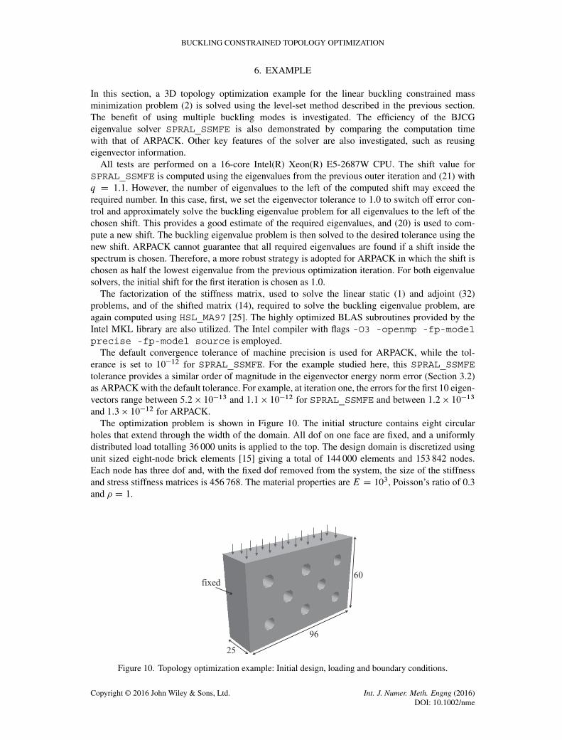
6. EXAMPLE
In this section, a 3D topology optimization example for the linear buckling constrained massminimization problem (2) is solved using the level-set method described in the previous section.The benefit of using multiple buckling modes is investigated. The efficiency of the BJCGeigenvalue solver SPRAL_SSMFE is also demonstrated by comparing the computation timewith that of ARPACK. Other key features of the solver are also investigated, such as reusingeigenvector information.
All tests are performed on a 16-core Intel(R) Xeon(R) E5-2687W CPU. The shift value forSPRAL_SSMFE is computed using the eigenvalues from the previous outer iteration and (21) withq D 1:1. However, the number of eigenvalues to the left of the computed shift may exceed therequired number. In this case, first, we set the eigenvector tolerance to 1.0 to switch off error con-trol and approximately solve the buckling eigenvalue problem for all eigenvalues to the left of thechosen shift. This provides a good estimate of the required eigenvalues, and (20) is used to com-pute a new shift. The buckling eigenvalue problem is then solved to the desired tolerance using thenew shift. ARPACK cannot guarantee that all required eigenvalues are found if a shift inside thespectrum is chosen. Therefore, a more robust strategy is adopted for ARPACK in which the shift ischosen as half the lowest eigenvalue from the previous optimization iteration. For both eigenvaluesolvers, the initial shift for the first iteration is chosen as 1.0.
The factorization of the stiffness matrix, used to solve the linear static (1) and adjoint (32)problems, and of the shifted matrix (14), required to solve the buckling eigenvalue problem, areagain computed using HSL_MA97 [25]. The highly optimized BLAS subroutines provided by theIntel MKL library are also utilized. The Intel compiler with flags -O3 -openmp -fp-modelprecise -fp-model source is employed.
The default convergence tolerance of machine precision is used for ARPACK, while the tol-erance is set to 10�12 for SPRAL_SSMFE. For the example studied here, this SPRAL_SSMFEtolerance provides a similar order of magnitude in the eigenvector energy norm error (Section 3.2)as ARPACK with the default tolerance. For example, at iteration one, the errors for the first 10 eigen-vectors range between 5:2 � 10�13 and 1:1 � 10�12 for SPRAL_SSMFE and between 1:2 � 10�13
and 1:3 � 10�12 for ARPACK.The optimization problem is shown in Figure 10. The initial structure contains eight circular
holes that extend through the width of the domain. All dof on one face are fixed, and a uniformlydistributed load totalling 36 000 units is applied to the top. The design domain is discretized usingunit sized eight-node brick elements [15] giving a total of 144 000 elements and 153 842 nodes.Each node has three dof and, with the fixed dof removed from the system, the size of the stiffnessand stress stiffness matrices is 456 768. The material properties are E D 103, Poisson’s ratio of 0.3and � D 1.
Figure 10. Topology optimization example: Initial design, loading and boundary conditions.
Copyright © 2016 John Wiley & Sons, Ltd. Int. J. Numer. Meth. Engng (2016)DOI: 10.1002/nme
P. D. DUNNING ET AL.
Table VII. Average (Ave.) times for SPRAL_SSMFE and ARPACK.
SPRAL_SSMFE Ave. time .s/No. modes Linear solve Shift-invert Buckle solve Adjoint solve Sub-problem outer iteration
5 17.4 19.3 44.8 12.4 0.5 96.810 17.3 19.2 49.5 12.2 4.0 108.825 17.4 19.8 82.7 28.3 26.3 183.8ARPACK
5 17.3 18.8 117.2 12.6 0.8 171.310 17.3 20.4 197.6 11.1 3.0 256.025 17.7 21.2 241.2 28.2 22.1 337.8
0
50
100
150
200
250
300
350
400
0 100 200 300
Buc
kle
solv
e ti
me
(s)
Iteration
ARPACK
SPRAL_SSMFE
Figure 11. Buckle solve time using 10 modes.
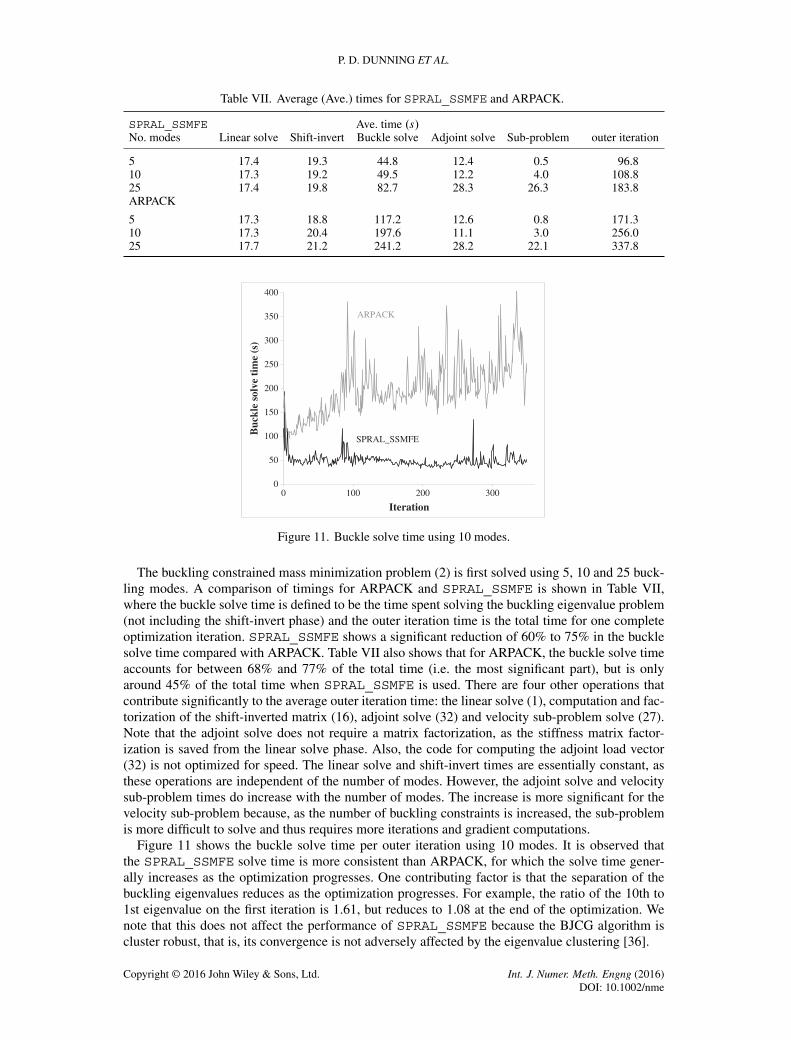
The buckling constrained mass minimization problem (2) is first solved using 5, 10 and 25 buck-ling modes. A comparison of timings for ARPACK and SPRAL_SSMFE is shown in Table VII,where the buckle solve time is defined to be the time spent solving the buckling eigenvalue problem(not including the shift-invert phase) and the outer iteration time is the total time for one completeoptimization iteration. SPRAL_SSMFE shows a significant reduction of 60% to 75% in the bucklesolve time compared with ARPACK. Table VII also shows that for ARPACK, the buckle solve timeaccounts for between 68% and 77% of the total time (i.e. the most significant part), but is onlyaround 45% of the total time when SPRAL_SSMFE is used. There are four other operations thatcontribute significantly to the average outer iteration time: the linear solve (1), computation and fac-torization of the shift-inverted matrix (16), adjoint solve (32) and velocity sub-problem solve (27).Note that the adjoint solve does not require a matrix factorization, as the stiffness matrix factor-ization is saved from the linear solve phase. Also, the code for computing the adjoint load vector(32) is not optimized for speed. The linear solve and shift-invert times are essentially constant, asthese operations are independent of the number of modes. However, the adjoint solve and velocitysub-problem times do increase with the number of modes. The increase is more significant for thevelocity sub-problem because, as the number of buckling constraints is increased, the sub-problemis more difficult to solve and thus requires more iterations and gradient computations.
Figure 11 shows the buckle solve time per outer iteration using 10 modes. It is observed thatthe SPRAL_SSMFE solve time is more consistent than ARPACK, for which the solve time gener-ally increases as the optimization progresses. One contributing factor is that the separation of thebuckling eigenvalues reduces as the optimization progresses. For example, the ratio of the 10th to1st eigenvalue on the first iteration is 1.61, but reduces to 1.08 at the end of the optimization. Wenote that this does not affect the performance of SPRAL_SSMFE because the BJCG algorithm iscluster robust, that is, its convergence is not adversely affected by the eigenvalue clustering [36].
Copyright © 2016 John Wiley & Sons, Ltd. Int. J. Numer. Meth. Engng (2016)DOI: 10.1002/nme
BUCKLING CONSTRAINED TOPOLOGY OPTIMIZATION
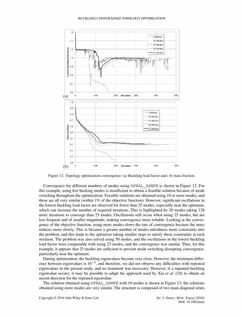
Figure 12. Topology optimization convergence: (a) Buckling load factor and ( b) mass fraction.
Convergence for different numbers of modes using SPRAL_SSMFE is shown in Figure 12. Forthis example, using five bucking modes is insufficient to obtain a feasible solution because of modeswitching throughout the optimization. Feasible solutions are obtained using 10 or more modes, andthese are all very similar (within 1% of the objective function). However, significant oscillations inthe lowest buckling load factor are observed for fewer than 25 modes, especially near the optimum,which can increase the number of required iterations. This is highlighted by 20 modes taking 128more iterations to converge than 25 modes. Oscillations still occur when using 25 modes, but areless frequent and of smaller magnitude, making convergence more reliable. Looking at the conver-gence of the objective function, using more modes slows the rate of convergence because the massreduces more slowly. This is because a greater number of modes introduces more constraints intothe problem, and this leads to the optimizer taking smaller steps to satisfy these constraints at eachiteration. The problem was also solved using 50 modes, and the oscillations in the lowest bucklingload factor were comparable with using 25 modes, and the convergence was similar. Thus, for thisexample, it appears that 25 modes are sufficient to prevent mode switching disrupting convergence,particularly near the optimum.
During optimization, the buckling eigenvalues become very close. However, the minimum differ-ence between eigenvalues is 10�5, and therefore, we did not observe any difficulties with repeatedeigenvalues in the present study, and no treatment was necessary. However, if a repeated bucklingeigenvalue occurs, it may be possible to adapt the approach used by Xia et al. [18] to obtain anascent direction for the repeated eigenvalue.
The solution obtained using SPRAL_SSMFE with 10 modes is shown in Figure 13; the solutionsobtained using more modes are very similar. The structure is composed of two main diagonal struts
Copyright © 2016 John Wiley & Sons, Ltd. Int. J. Numer. Meth. Engng (2016)DOI: 10.1002/nme
P. D. DUNNING ET AL.
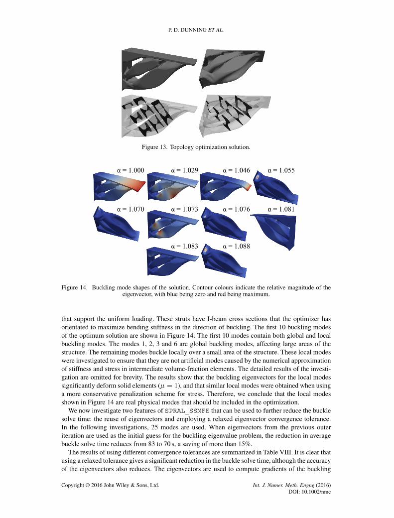
Figure 13. Topology optimization solution.
Figure 14. Buckling mode shapes of the solution. Contour colours indicate the relative magnitude of theeigenvector, with blue being zero and red being maximum.
that support the uniform loading. These struts have I-beam cross sections that the optimizer hasorientated to maximize bending stiffness in the direction of buckling. The first 10 buckling modesof the optimum solution are shown in Figure 14. The first 10 modes contain both global and localbuckling modes. The modes 1, 2, 3 and 6 are global buckling modes, affecting large areas of thestructure. The remaining modes buckle locally over a small area of the structure. These local modeswere investigated to ensure that they are not artificial modes caused by the numerical approximationof stiffness and stress in intermediate volume-fraction elements. The detailed results of the investi-gation are omitted for brevity. The results show that the buckling eigenvectors for the local modessignificantly deform solid elements (� D 1), and that similar local modes were obtained when usinga more conservative penalization scheme for stress. Therefore, we conclude that the local modesshown in Figure 14 are real physical modes that should be included in the optimization.
We now investigate two features of SPRAL_SSMFE that can be used to further reduce the bucklesolve time: the reuse of eigenvectors and employing a relaxed eigenvector convergence tolerance.In the following investigations, 25 modes are used. When eigenvectors from the previous outeriteration are used as the initial guess for the buckling eigenvalue problem, the reduction in averagebuckle solve time reduces from 83 to 70 s, a saving of more than 15%.
The results of using different convergence tolerances are summarized in Table VIII. It is clear thatusing a relaxed tolerance gives a significant reduction in the buckle solve time, although the accuracyof the eigenvectors also reduces. The eigenvectors are used to compute gradients of the buckling
Copyright © 2016 John Wiley & Sons, Ltd. Int. J. Numer. Meth. Engng (2016)DOI: 10.1002/nme
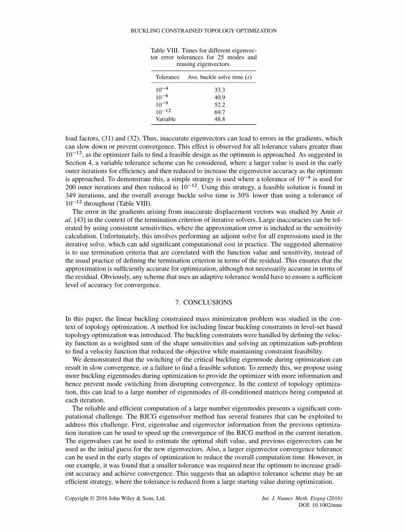
BUCKLING CONSTRAINED TOPOLOGY OPTIMIZATION
Table VIII. Times for different eigenvec-tor error tolerances for 25 modes and
reusing eigenvectors.
Tolerance Ave. buckle solve time .s/
10�4 33.310�6 40.910�9 52.210�12 69.7Variable 48.8
load factors, (31) and (32). Thus, inaccurate eigenvectors can lead to errors in the gradients, whichcan slow down or prevent convergence. This effect is observed for all tolerance values greater than10�12, as the optimizer fails to find a feasible design as the optimum is approached. As suggested inSection 4, a variable tolerance scheme can be considered, where a larger value is used in the earlyouter iterations for efficiency and then reduced to increase the eigenvector accuracy as the optimumis approached. To demonstrate this, a simple strategy is used where a tolerance of 10�4 is used for200 outer iterations and then reduced to 10�12. Using this strategy, a feasible solution is found in349 iterations, and the overall average buckle solve time is 30% lower than using a tolerance of10�12 throughout (Table VIII).
The error in the gradients arising from inaccurate displacement vectors was studied by Amir etal. [43] in the context of the termination criterion of iterative solvers. Large inaccuracies can be tol-erated by using consistent sensitivities, where the approximation error is included in the sensitivitycalculation. Unfortunately, this involves performing an adjoint solve for all expressions used in theiterative solve, which can add significant computational cost in practice. The suggested alternativeis to use termination criteria that are correlated with the function value and sensitivity, instead ofthe usual practice of defining the termination criterion in terms of the residual. This ensures that theapproximation is sufficiently accurate for optimization, although not necessarily accurate in terms ofthe residual. Obviously, any scheme that uses an adaptive tolerance would have to ensure a sufficientlevel of accuracy for convergence.
7. CONCLUSIONS
In this paper, the linear buckling constrained mass minimizaton problem was studied in the con-text of topology optimization. A method for including linear buckling constraints in level-set basedtopology optimization was introduced. The buckling constraints were handled by defining the veloc-ity function as a weighted sum of the shape sensitivities and solving an optimization sub-problemto find a velocity function that reduced the objective while maintaining constraint feasibility.
We demonstrated that the switching of the critical buckling eigenmode during optimization canresult in slow convergence, or a failure to find a feasible solution. To remedy this, we propose usingmore buckling eigenmodes during optimization to provide the optimizer with more information andhence prevent mode switching from disrupting convergence. In the context of topology optimiza-tion, this can lead to a large number of eigenmodes of ill-conditioned matrices being computed ateach iteration.
The reliable and efficient computation of a large number eigenmodes presents a significant com-putational challenge. The BJCG eigensolver method has several features that can be exploited toaddress this challenge. First, eigenvalue and eigenvector information from the previous optimiza-tion iteration can be used to speed up the convergence of the BJCG method in the current iteration.The eigenvalues can be used to estimate the optimal shift value, and previous eigenvectors can beused as the initial guess for the new eigenvectors. Also, a larger eigenvector convergence tolerancecan be used in the early stages of optimization to reduce the overall computation time. However, inour example, it was found that a smaller tolerance was required near the optimum to increase gradi-ent accuracy and achieve convergence. This suggests that an adaptive tolerance scheme may be anefficient strategy, where the tolerance is reduced from a large starting value during optimization.
Copyright © 2016 John Wiley & Sons, Ltd. Int. J. Numer. Meth. Engng (2016)DOI: 10.1002/nme
P. D. DUNNING ET AL.
A 3D optimization problem was used to demonstrate the effectiveness of the level-set topologyoptimization method and the efficiency of the BJCG eigenvalue solver, implemented in the packageSPRAL_SSMFE. The level-set method was able to obtain feasible designs for the mass minimizationproblem with as many as 50 linear buckling constraints. Buckling eigenvalue solution times usingSPRAL_SSMFE were compared with APRACK. The results show that a significant reduction inthe buckling solve time can be achieved by using SPRAL_SSMFE, especially when eigenvalue andeigenvector information is reused and an adaptive eigenvector tolerance scheme employed. For avery large number of modes, SPRAL_SSMFE can also employ a multiple shift strategy to furtherreduce overall computation time.
ACKNOWLEDGEMENTS
The authors acknowledge the support from the Engineering and Physical Sciences Research Council, fel-lowship grants EP/M002322/1 and EP/J010553/1. We also thank Dr Bret Stanford (NASA Langley) foruseful discussions.
REFERENCES
1. Haftka RT, Gürdal Z. Elements of Structural Optimization (Third Revised and Expanded edn.) Kluwer AcademicPublishers: Dordrecht, 1992.
2. Spillers WR, MacBain KM. Structural Optimization. Springer: Dordrecht, 2009.3. Deaton JD, Grandhi RV. A survey of structural and multidisciplinary continuum topology optimization: post 2000.
Structural and Multidisciplinary Optimization 2014; 49(1):1–38.4. Sigmund O, Maute K. Topology optimization approaches a comparative review. Structural and Multidisciplinary
Optimization 2013; 48(6):1031–1055.5. Rozvany GIN. Difficulties in truss topology optimization with stress, local buckling and system stability constraints.
Structural Optimization 1996; 11(3-4):213–217.6. Zhou M. Difficulties in truss topology optimization with stress and local buckling constraints. Structural Optimization
1996; 11(2):134–136.7. Kocvara M. On the modelling and solving of the truss design problem with global stability constraints. Structural
and Multidisciplinary Optimization 2002; 23(3):189–203.8. Rahmatalla S, Swan CC. Continuum topology optimization of buckling-sensitive structures. AIAA Journal 2003;
41(6):1180–1189.9. Lund E. Buckling topology optimization of laminated multi-material composite shell structures. Composite Struc-
tures 2009; 91(2):158–167.10. Rong JH, Xie YM, Yang XY. An improved method for evolutionary structural optimisation against buckling.
Computers and Structures 2001; 79(3):253–263.11. Neves MM, Rodrigues H, Guedes JM. Generalized topology design of structures with a buckling load criterion.
Structural Optimization 1995; 10(2):71–78.12. Lindgaard E, Dahl J. On compliance and buckling objective functions in topology optimization of snap-through
problems. Structural and Multidisciplinary Optimization 2013; 47(3):409–421.13. Allaire G, Jouve F, Toader AM. Structural optimization using sensitivity analysis and a level-set method. Journal of
Computational Physics 2004; 194(1):363–393.14. Wang MY, Wang X, Guo D. A level set method for structural topology optimization. Computer Methods in Applied
Mechanics and Engineering 2003; 192(1-2):227–246.15. Cook RD, Malkus DS, Plesha ME, Witt RJ. Concepts and applications of finite element analysis (4th edn). John
Wiley & Sons, Inc.: United States, 2002.16. Bruyneel M, Colson B, Remouchamps A. Discussion on some convergence problems in buckling optimisation.
Structural and Multidisciplinary Optimization 2008; 35(2):181–186.17. Seyranian AP, Lund E, Olhoff N. Multiple-eigenvalues in structural optimization problems. Structural Optimization
1994; 8(4):207–227.18. Xia Q, Shi T, Wang MY. A level set based shape and topology optimization method for maximizing the simple or
repeated first eigenvalue of structure vibration. Structural and Multidisciplinary Optimization 2011; 43(4):473–485.19. Dunning PD, Stanford BK, Kim HA. Level-set topology optimization with aeroelastic constraints. 56th
AIAA/ASCE/AHS/ASC Structures, Structural Dynamics, and Materials Conference, AIAA SciTech, AmericanInstitute of Aeronautics and Astronautics, Kissimmee, Florida, USA, 2015; 1–19.
20. Wang S, de Sturler E, Paulino GH. Large-scale topology optimization using preconditioned Krylov subspace methodswith recycling. International Journal for Numerical Methods in Engineering 2007; 69(12):2441–2468.
21. Makhija D, Maute K. Numerical instabilities in level set topology optimization with the extended finite elementmethod. Structural and Multidisciplinary Optimization 2014; 49(2):185–197.
22. Lehoucq RB, Sorensen DC, Yang C. ARPACK Users Guide: Solution of Large-Scale Eigenvalue Problems withImplicitly Restarted Arnoldi Methods. SIAM: Philadelphia, 1998.
Copyright © 2016 John Wiley & Sons, Ltd. Int. J. Numer. Meth. Engng (2016)DOI: 10.1002/nme
BUCKLING CONSTRAINED TOPOLOGY OPTIMIZATION
23. MATLAB. version 8.2.0.701 (r2013b). The MathWorks Inc.: Natick, Massachusetts, 2013.24. The NAG library. The Numerical Algorithms Group (NAG), Oxford, United Kingdom. (Available from: http://www.
nag.com) [Accessed on 1 May 2015].25. Hogg JD, Scott JA. HSL_MA97: a bit-compatible multifrontal code for sparse symmetric systems. Technical Report
RAL-TR-2011-024, Rutherford Appleton Laboratory: Harwell Oxford, Didcot, Oxfordshire, UK, 2011.26. HSL. A collection of Fortran codes for large-scale scientific computation, 2013. (Available from: http://www.hsl.rl.
ac.uk) [Accessed on 1 May 2015].27. SPRAL. Sparse parallel robust algorithms library, 2015. (Available from: http://www.numerical.rl.ac.uk/spral/)
[Accessed on 1 May 2015].28. O’Leary DP. The block conjugate gradient algorithm and related methods. Linear Algebra and its Applications 1980;
29:293–322.29. Arbenz P, Hetmaniuk UL, Lehoucq RB, Tuminaro RS. A comparison of eigensolvers for large-scale 3D modal
analysis using AMG-preconditioned iterative methods. International Journal for Numerical Methods in Engineering2005; 64(2):204–236.
30. Knyazev AV. Toward the optimal preconditioned eigensolver: locally optimal block preconditioned conjugategradient method. SIAM Journal on Scientific Computing 2001; 23(2):517–541.
31. Kraft D. A software package for sequential quadratic programming. Technical Report DFVLR-FB 88-28, Institut fürDynamik der Flugsysteme: Oberpfaffenhofen, 1988.
32. Kraft D. TOMP - Fortran modules for optimal control calculations. ACM Transactions on Mathematical Software1994; 20(3):262–281.
33. The NLopt nonlinear optimization package, 2014. (Available from: http://ab-initio.mit.edu/nlopt) [Accessed on1 May 2015].
34. van Zyl LH. Use of eigenvectors in the solution of the flutter equation. Journal of Aircraft 1993; 30(4):553–554.35. Ovtchinnikov EE. Jacobi correction equation, line search and conjugate gradients in Hermitian eigenvalue computa-
tion I: Computing an extreme eigenvalue. SIAM Journal on Numerical Analysis 2008; 46(5):2567–2592.36. Ovtchinnikov EE. Jacobi correction equation, line search and conjugate gradients in Hermitian eigenvalue
computation II: Computing several extreme eigenvalues. SIAM Journal on Numerical Analysis 2008; 46(5):2593–2619.
37. Ovtchinnikov EE. Computing several eigenpairs of Hermitian problems by conjugate gradient iterations. Journal ofComputational Physics 2008; 227(22):9477–9497.
38. Takahashi I. A note on the conjugate gradient method. Information Processing in Japan 1965; 5:45–49.39. Saad Y. Projection methods for solving large sparse eigenvalue problems. Lecture Notes in Mathematics 1983;
973:121–144.40. Dunning PD, Stanford BK, Kim HA. Coupled aerostructural topology optimization using a level set method for 3D
aircraft wings. Structural and Multidisciplinary Optimization 2015; 51(5):1113–1132.41. Dunning PD, Kim HA. Introducing the sequential linear programming level-set method for topology optimization.
Structural and Multidisciplinary Optimization 2015; 51(3):631–643.42. Dunning PD, Kim HA, Mullineux G. Investigation and improvement of sensitivity computation using the area-
fraction weighted fixed grid FEM and structural optimization. Finite Elements in Analysis and Design 2011;47(8):933–941.
43. Amir O, Stolpe M, Sigmund O. Efficient use of iterative solvers in nested topology optimization. Structural andMultidisciplinary Optimization 2010; 42(1):55–72.
Copyright © 2016 John Wiley & Sons, Ltd. Int. J. Numer. Meth. Engng (2016)DOI: 10.1002/nme