
Lessons from OECD forecasts during and after the financial ...€¦ · Lessons from OECD forecasts...
31
OECD Journal: Economic Studies Volume 2014 © OECD 2015 9 Lessons from OECD forecasts during and after the financial crisis by Christine Lewis and Nigel Pain* This paper assesses the OECD’s projections for GDP growth and inflation during the global financial crisis and recovery, focusing on lessons that can be learned. Growth was repeatedly overestimated in the projections, which failed to anticipate the extent of the slowdown and later the weak pace of the recovery. Similar errors were made by many other forecasters. At the same time, inflation was stronger than expected on average. Analysis of the growth errors shows that the OECD projections in the crisis years were larger in countries with more international trade openness and greater presence of foreign banks. In the recovery, there is little evidence that an underestimate of the impact of fiscal consolidation contributed significantly to forecast errors. Instead, the repeated conditioning assumption that the euro area crisis would stabilise or ease played an important role, with growth weaker than projected in European countries where bond spreads were higher than had been assumed. But placing these errors in a historical context illustrates that the errors were not without precedent: similar-sized errors were made in the first oil price shock of the 1970s. In response to the challenges encountered in forecasting in recent years and the lessons learnt, the OECD and other international organisations have sought to improve their forecasting techniques and procedures, to improve their ability to monitor near-term developments and to better account for international linkages and financial market developments. JEL classification: E17, E27, E32, E37, E62, E66, F47, G01 Keywords: Forecasting, economic outlook, economic fluctuations, fiscal policy * This article is drawn from a wider project on OECD forecasts undertaken with Thai Thanh Dang, Yosuke Jin and Pete Richardson; we are grateful for their help.The authors also wish to thank Jørgen Elmeskov, Jean-Luc Schneider, Sveinbjörn Blöndal, other colleagues in the OECD Economics Department, Prakash Loungani and Volker Ziemann for comments on earlier drafts and Jérôme Brézillon for statistical assistance. The statistical data for Israel are supplied by and under the responsibility of the relevant Israeli authorities. The use of such data by the OECD is without prejudice to the status of the Golan Heights, East Jerusalem and Israeli settlements in theWest Bank under the terms of international law.
Transcript of Lessons from OECD forecasts during and after the financial ...€¦ · Lessons from OECD forecasts...
OECD Journal: Economic Studies
Volume 2014
© OECD 2015
9
Lessons from OECD forecasts duringand after the financial crisis
byChristine Lewis and Nigel Pain*
This paper assesses the OECD’s projections for GDP growth and inflation during theglobal financial crisis and recovery, focusing on lessons that can be learned. Growthwas repeatedly overestimated in the projections, which failed to anticipate theextent of the slowdown and later the weak pace of the recovery. Similar errors weremade by many other forecasters. At the same time, inflation was stronger thanexpected on average. Analysis of the growth errors shows that the OECD projectionsin the crisis years were larger in countries with more international trade opennessand greater presence of foreign banks. In the recovery, there is little evidence that anunderestimate of the impact of fiscal consolidation contributed significantly toforecast errors. Instead, the repeated conditioning assumption that the euro areacrisis would stabilise or ease played an important role, with growth weaker thanprojected in European countries where bond spreads were higher than had beenassumed. But placing these errors in a historical context illustrates that the errorswere not without precedent: similar-sized errors were made in the first oil priceshock of the 1970s. In response to the challenges encountered in forecasting in recentyears and the lessons learnt, the OECD and other international organisations havesought to improve their forecasting techniques and procedures, to improve theirability to monitor near-term developments and to better account for internationallinkages and financial market developments.
JEL classification: E17, E27, E32, E37, E62, E66, F47, G01
Keywords: Forecasting, economic outlook, economic fluctuations, fiscal policy
* This article is drawn from a wider project on OECD forecasts undertaken with Thai Thanh Dang,Yosuke Jin and Pete Richardson; we are grateful for their help. The authors also wish to thank JørgenElmeskov, Jean-Luc Schneider, Sveinbjörn Blöndal, other colleagues in the OECD EconomicsDepartment, Prakash Loungani and Volker Ziemann for comments on earlier drafts and JérômeBrézillon for statistical assistance.The statistical data for Israel are supplied by and under the responsibility of the relevant Israeliauthorities. The use of such data by the OECD is without prejudice to the status of the Golan Heights,East Jerusalem and Israeli settlements in the West Bank under the terms of international law.
LESSONS FROM OECD FORECASTS DURING AND AFTER THE FINANCIAL CRISIS
OECD JOURNAL: ECONOMIC STUDIES – VOLUME 2014 © OECD 201510
1. Introduction and summaryThis paper assesses the performance of OECD projections for GDP growth over the
period 2007-12 and places these in the context of the errors made in earlier years and by
other international organisations. The focus is on the lessons that can be learned from
projection errors and their cross-country differences and the resulting changes to
forecasting models and procedures that have occurred since the start of the financial crisis,
both inside the OECD and in other international organisations.
Forecasting the timing, depth and ramifications of the global financial crisis proved
exceptionally difficult. Particular challenges included the identification of imbalances and
unsustainabilities entering the crisis, the timing of their unwinding and the likely impact
on real activity. These challenges were compounded by the unusually high speed and
depth of cross-country interconnections between real and financial developments, the
increased variability of economic growth compared with the pre-crisis period, the lack of
timely data on many important financial factors and the limited understanding of macro-
financial linkages. All these came on top of the well documented difficulties normally
experienced when forecasting around major turning points in activity.
On average across the OECD and the BRIICS economies, calendar year GDP growth was
overestimated across 2007-12, with the largest errors occurring in the projections for the
vulnerable euro area economies. The largest errors were made at the height of the financial
crisis in 2009 but there were also growth disappointments during the recovery. The OECD
was not alone in finding this period particularly challenging. The profile and magnitude of
the errors in the GDP growth projections of other international organisations and
consensus forecasts are strikingly similar.
Although recent projection errors were large, they were not unprecedented: the first
oil-price shock in the early 1970s also proved to be an equally difficult period for
forecasters. Over a longer perspective of forty years, the OECD projections for G7 countries
have generally been efficient and informative. Allowing for variations in growth volatility
over time, the projection errors over 2007-12 are of a broadly similar magnitude to those in
the pre-crisis years.
A number of economic characteristics are associated with the projection errors during
this period. Growth was typically weaker than expected and errors higher in countries that
are more open to external developments and exposed to shocks from other economies. For
example, international trade openness and the presence of foreign banks in the economy
are strongly associated with larger errors during the downturn period. This suggests that
the projections may have failed to fully reflect the higher exposure of these economies to
interconnected negative global shocks. In the recovery, growth was weaker than expected
in countries in which banks had low pre-crisis capital ratios and in countries in which non-
performing loans had risen strongly. Moreover, growth in countries with more regulated
product and labour markets has generally proved more difficult to forecast. In part this
LESSONS FROM OECD FORECASTS DURING AND AFTER THE FINANCIAL CRISIS
OECD JOURNAL: ECONOMIC STUDIES – VOLUME 2014 © OECD 2015 11
may reflect insufficient attention being paid to the extent to which tighter regulations have
delayed the necessary reallocation across sectors in the recovery phase.
Based on the OECD forecasts, stronger projected fiscal consolidation has been
associated with growth disappointments, but only in some years and only if Greece is
included in the sample used. The repeated assumption that the euro crisis would dissipate
over time, and that sovereign bond yield differentials would narrow, appears to have been
a more important source of error. This underlines the conditional nature of OECD
projections, which are not intended to be forecasts, but also raises questions about the
conditioning assumptions chosen.
In response to the crisis, the OECD and other international organisations have been
reviewing and changing their forecast procedures and practices. A key change has been to
increase the centralisation of the early stages of the forecast round. This ensures that
global economic developments and cross-country spillover effects are reflected
consistently in the projections for individual economies. Monitoring and statistical
modelling of near-term developments has also been enhanced, with the OECD’s indicator
models for near-term GDP and global trade growth proving to be a useful source of
guidance. Anecdotal evidence from contacts with businesses has also become more
important. In addition, there is now a stronger focus on financial market developments,
with financial market indicators increasingly being integrated into projection processes
and macroeconomic models. Communication efforts have also been enhanced to
characterise the shape of the risk distribution around the baseline projection, including
forecast ranges and the use of fan charts. Greater use is also being made of quantitative
scenario analyses to illustrate the implications of key risks.
The structure of this paper is as follows. Section 2 briefly reviews forecasting and risk
assessment practices before the onset of the financial crisis and then discusses the
properties of the errors made for the 2007-12 period. (The focus is on the period of the crisis
and the years that immediately followed because this paper is based on a project covering
those years (Pain, et al., 2014); 2013 is not reported in the paper but revisions to the initial
projections were generally comparatively small.) Section 3 assesses whether OECD
projection errors in the 2007-12 period, or the downturn and recovery sub-periods, are
systematically linked to pre-crisis conditions, structural conditions, and policy
assumptions. Section 4 places the recent errors in a longer-run context to better
understand whether they are unusual errors from an unusual period. A discussion of the
nature of the projections follows. The final part of the paper takes stock of recent changes
in forecasting procedures and practices in the OECD and other international organisations
to address the identified weaknesses with earlier forecasting practices, drawing on a series
of interviews undertaken in 2013. Information on the data set used and the statistical
procedures undertaken is summarised in Box 1.
2. Forecasting before and during the crisis
2.1. Forecasting and risk assessment practices before the onset of the financial crisis
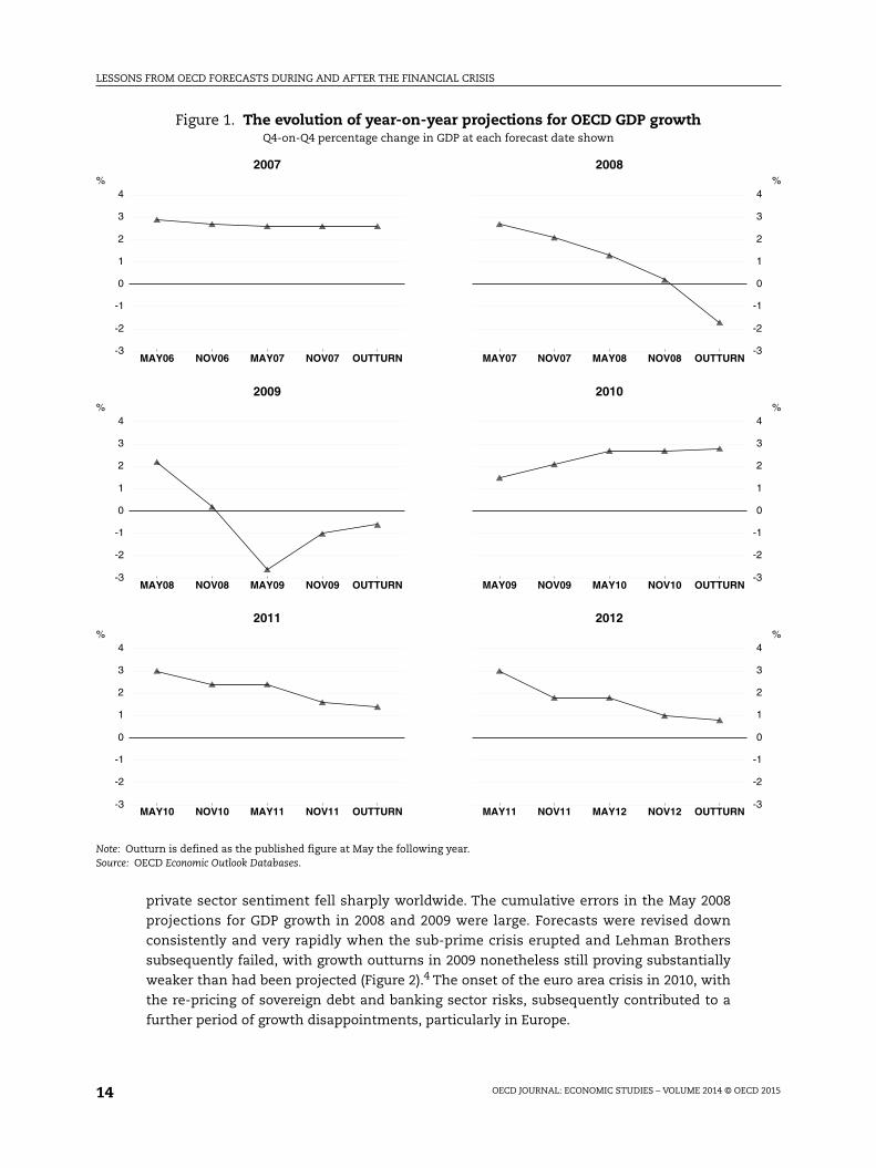
The pre-crisis period was one of relative economic stability. OECD projections in this
period appeared to perform relatively well (Vogel, 2007), with only limited revisions to GDP
growth projections typically observed as the forecast horizon narrowed, even for 2007
(Figure 1).1 However, changes in the global economy and financial system in the early to
mid-2000s contributed to the subsequent difficulties of forecasting once the crisis began.
LESSONS FROM OECD FORECASTS DURING AND AFTER THE FINANCIAL CRISIS
OECD JOURNAL: ECONOMIC STUDIES – VOLUME 2014 © OECD 201512
Box 1. Data and definitions
Data
The results in this document make use of data sets for projections made by the OECD for OECD countriesand six non-member countries (the BRIICS: Brazil, Russia, India, Indonesia, China and South Africa), withthe main focus on OECD countries. Annual calendar year GDP growth data for 2007-12 are used for allcountries except India, where annual growth over the fiscal year (to April) is used. Three different sets ofprojections are considered:
● May Economic Outlook projections for calendar year GDP growth and inflation in the same year.
● May Economic Outlook projections for calendar year GDP growth and inflation in the following year.
● November Economic Outlook projections for calendar year GDP growth and inflation in the following year.
The projection error is defined as the outturn less the projection. The outturn data for GDP growth in anygiven year are taken from the May Economic Outlook in the year immediately after. An issue for allevaluations of forecasting performance is the appropriate vintage of data to use, since the initial outturnestimates may not be especially reliable, particularly at times of rapid change in the economy (Shresthaand Marini, 2013). But use of the latest vintages of data can result in the calculated forecast errors beingmisleading, since they can also contain changes to national accounting procedures and concepts that werenot known about at the time of the projection. This paper follows standard practice in using earlyrealisations of the outcome.
To enable longer-run comparisons, OECD growth projections for the G7 countries from 1971 are also used.For some countries, these include GNP growth projections, rather than GDP growth, over the first part of thesample period.
Use is also made of a short-run and longer-run dataset of other forecasters’ projections for GDP growthin the G7 countries. The short dataset, covering 2007-12, includes projections published by the IMF,European Commission and Consensus Economics, where the latter is the average of private-sectoreconomists’ forecasts for each country. The longer-run dataset for the G7 countries, covering 1991-2012,also includes consensus forecasts from 1991 onwards.
Key metrics
The paper uses three key measures of the size of the errors:
● The average error for each country, which is the average projection error (defined as above) over a givenperiod. The means for various country groups are based on unweighted averages across countries andtime.
● The average absolute error, defined as the average of the absolute value of individual country errors overthe time period shown. For country groups, this is calculated as the unweighted average of absoluteerrors across countries and time. For greater comparability across countries and time, the averageabsolute error is also scaled by the corresponding average absolute growth rates. The ratio of countrygroups is calculated as the unweighted average ratio across countries.
● The root mean squared error (RMSE), which is calculated by squaring individual country errors, thenaveraging these over the time period shown and taking the square root of the result. For country groups,this is the square root of the average of country squared errors, where the average is calculated acrosscountries and time. To improve comparability, the RMSE is also scaled by the average volatility of growth(i.e. standard deviations) for a country or time period. The ratio of country groups is calculated as theunweighted average across countries.
LESSONS FROM OECD FORECASTS DURING AND AFTER THE FINANCIAL CRISIS
OECD JOURNAL: ECONOMIC STUDIES – VOLUME 2014 © OECD 2015 13
This period was one of increasing globalisation and integration of real and financial
activity, raising the potential for cross-border and cross-market transmission of economic
and financial shocks. Foreign-owned banks became more important in domestic banking
markets and in many economies bank funding relied increasingly on international
markets. Financial leverage and risk-taking expanded rapidly in a low interest rate
environment, reflected in strong asset price and credit growth. External imbalances also
built up to what were widely viewed as unsustainable levels.
Limited weight was given to the possible impact of excessive risk-taking in the
projections made before the crisis, not least because the extent of risk-taking was often
hidden in off-balance-sheet activities or masked by derivative positions. That said,
frequent risk analysis was done of the extent of over-valuation of housing markets and the
activity implications stemming from developments such as the run-up and subsequent
correction in US house prices.2 However, only a handful of financial variables were
integrated fully into the forecast process and the background models used; typically,
account was taken only of policy interest rate and asset price effects on activity.3 Certain
structural policy settings, notably less stringent product and labour market regulations,
were believed to enhance the resilience of economies by improving the flexibility to bounce
back relatively quickly from downturns, conditional on the assumption that financial
markets and the monetary transmission mechanism functioned in a normal manner
(Duval et al., 2007; Duval and Vogel, 2008). In this context, increases in financial depth were
seen as being beneficial to both long-term growth and cyclical resilience.
2.2. Forecast performance during the financial crisis and its aftermath: GDP growth
As the crisis intensified, it spread across countries rapidly, in a manner well beyond
that suggested by the linkages built into standard forecasting and simulation models
(Bini Smaghi, 2010). Global trade collapsed in late 2008 and the early part of 2009, and
Box 1. Data and definitions (cont.)
Forecast evaluation tests
● Unbiasedness: tested by a pooled regression of country projection errors on a constant. Unbiasednessrequires that = 0 in:
Errorit = + it [1]● Information content: tested by a pooled regression. Informative projections have positive in:
Outcomeit = + Projectionit +it [2]Information content is also tested relative to two alternative forecasts: a naïve forecast of the previousyear’s growth rate; and the consensus forecasts.
● Efficiency: this can be measured in several ways, with different degrees of strength. A basic requirementis simply that the RMSE is smaller at each forecast horizon. A slightly stronger definition is that the errorshould not be predictable and the projections should be informative – “weak efficiency” – which requiresthat both = 0 and = 1 in the second regression above. A third, stronger form of efficiency is thatprojections embody all information available to the forecasters at the time, in which case the projectionerrors should be uncorrelated with informative data series. Another strong test of efficiency requiresthat revisions to a specific forecast be small and unpredictable from one forecasting round to the next,and uncorrelated with the previous revision.
● Directional accuracy: this measures whether the projections were qualitatively accurate, in the sense ofaccurately projecting rising or declining growth rates in the forecast period.
LESSONS FROM OECD FORECASTS DURING AND AFTER THE FINANCIAL CRISIS
OECD JOURNAL: ECONOMIC STUDIES – VOLUME 2014 © OECD 201514
private sector sentiment fell sharply worldwide. The cumulative errors in the May 2008
projections for GDP growth in 2008 and 2009 were large. Forecasts were revised down
consistently and very rapidly when the sub-prime crisis erupted and Lehman Brothers
subsequently failed, with growth outturns in 2009 nonetheless still proving substantially
weaker than had been projected (Figure 2).4 The onset of the euro area crisis in 2010, with
the re-pricing of sovereign debt and banking sector risks, subsequently contributed to a
further period of growth disappointments, particularly in Europe.
Figure 1. The evolution of year-on-year projections for OECD GDP growthQ4-on-Q4 percentage change in GDP at each forecast date shown
Note: Outturn is defined as the published figure at May the following year.Source: OECD Economic Outlook Databases.
MAY06 NOV06 MAY07 NOV07 OUTTURN-3
-2
-1
0
1
2
3
4%
2007
MAY08 NOV08 MAY09 NOV09 OUTTURN-3
-2
-1
0
1
2
3
4%
2009
MAY10 NOV10 MAY11 NOV11 OUTTURN-3
-2
-1
0
1
2
3
4%
2011
MAY07 NOV07 MAY08 NOV08 OUTTURN
-3
-2
-1
0
1
2
3
4%
2008
MAY09 NOV09 MAY10 NOV10 OUTTURN
-3
-2
-1
0
1
2
3
4%
2010
MAY11 NOV11 MAY12 NOV12 OUTTURN
-3
-2
-1
0
1
2
3
4%
2012
LESSONS FROM OECD FORECASTS DURING AND AFTER THE FINANCIAL CRISIS
OECD JOURNAL: ECONOMIC STUDIES – VOLUME 2014 © OECD 2015 15
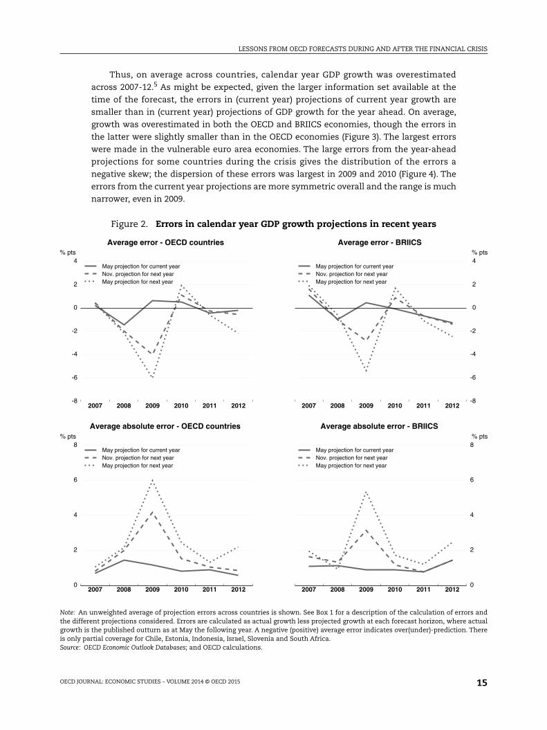
Thus, on average across countries, calendar year GDP growth was overestimated
across 2007-12.5 As might be expected, given the larger information set available at the
time of the forecast, the errors in (current year) projections of current year growth are
smaller than in (current year) projections of GDP growth for the year ahead. On average,
growth was overestimated in both the OECD and BRIICS economies, though the errors in
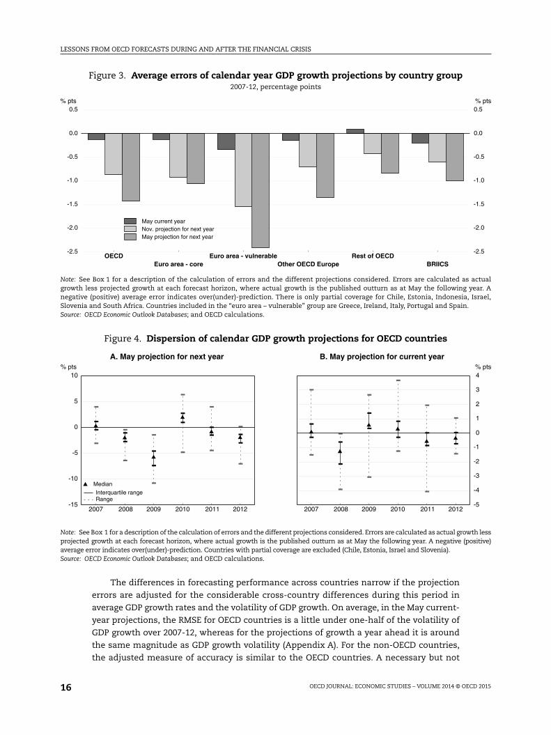
the latter were slightly smaller than in the OECD economies (Figure 3). The largest errors
were made in the vulnerable euro area economies. The large errors from the year-ahead
projections for some countries during the crisis gives the distribution of the errors a
negative skew; the dispersion of these errors was largest in 2009 and 2010 (Figure 4). The
errors from the current year projections are more symmetric overall and the range is much
narrower, even in 2009.
Figure 2. Errors in calendar year GDP growth projections in recent years
Note: An unweighted average of projection errors across countries is shown. See Box 1 for a description of the calculation of errors andthe different projections considered. Errors are calculated as actual growth less projected growth at each forecast horizon, where actualgrowth is the published outturn as at May the following year. A negative (positive) average error indicates over(under)-prediction. Thereis only partial coverage for Chile, Estonia, Indonesia, Israel, Slovenia and South Africa.Source: OECD Economic Outlook Databases; and OECD calculations.
2007 2008 2009 2010 2011 2012-8
-6
-4
-2
0
2
4% pts
May projection for current yearNov. projection for next yearMay projection for next year
Average error - OECD countries
2007 2008 2009 2010 2011 20120
2
4
6
8% pts
May projection for current yearNov. projection for next yearMay projection for next year
Average absolute error - OECD countries
2007 2008 2009 2010 2011 2012
-8
-6
-4
-2
0
2
4% pts
May projection for current yearNov. projection for next yearMay projection for next year
Average error - BRIICS
2007 2008 2009 2010 2011 2012
0
2
4
6
8% pts
May projection for current yearNov. projection for next yearMay projection for next year
Average absolute error - BRIICS
LESSONS FROM OECD FORECASTS DURING AND AFTER THE FINANCIAL CRISIS
OECD JOURNAL: ECONOMIC STUDIES – VOLUME 2014 © OECD 201516
The differences in forecasting performance across countries narrow if the projection
errors are adjusted for the considerable cross-country differences during this period in
average GDP growth rates and the volatility of GDP growth. On average, in the May current-
year projections, the RMSE for OECD countries is a little under one-half of the volatility of
GDP growth over 2007-12, whereas for the projections of growth a year ahead it is around
the same magnitude as GDP growth volatility (Appendix A). For the non-OECD countries,
the adjusted measure of accuracy is similar to the OECD countries. A necessary but not
Figure 3. Average errors of calendar year GDP growth projections by country group2007-12, percentage points
Note: See Box 1 for a description of the calculation of errors and the different projections considered. Errors are calculated as actualgrowth less projected growth at each forecast horizon, where actual growth is the published outturn as at May the following year. Anegative (positive) average error indicates over(under)-prediction. There is only partial coverage for Chile, Estonia, Indonesia, Israel,Slovenia and South Africa. Countries included in the “euro area – vulnerable” group are Greece, Ireland, Italy, Portugal and Spain.Source: OECD Economic Outlook Databases; and OECD calculations.
Figure 4. Dispersion of calendar GDP growth projections for OECD countries
Note: See Box 1 for a description of the calculation of errors and the different projections considered. Errors are calculated as actual growth lessprojected growth at each forecast horizon, where actual growth is the published outturn as at May the following year. A negative (positive)average error indicates over(under)-prediction. Countries with partial coverage are excluded (Chile, Estonia, Israel and Slovenia).Source: OECD Economic Outlook Databases; and OECD calculations.
OECD Euro area - vulnerable Rest of OECDEuro area - core Other OECD Europe BRIICS
-2.5
-2.0
-1.5
-1.0
-0.5
0.0
0.5% pts
-2.5
-2.0
-1.5
-1.0
-0.5
0.0
0.5% pts
May current yearNov. projection for next yearMay projection for next year
2007 2008 2009 2010 2011 2012-15
-10
-5
0
5
10% pts
-- -
--
---
-
-- --
--
-- --
--
- --
Interquartile rangeRange
Median
A. May projection for next year
2007 2008 2009 2010 2011 2012
-5
-4
-3
-2
-1
0
1
2
3
4% pts
-
-
--
---
-
- -- --
-
- - - --
--
-
-
-
B. May projection for current year
LESSONS FROM OECD FORECASTS DURING AND AFTER THE FINANCIAL CRISIS
OECD JOURNAL: ECONOMIC STUDIES – VOLUME 2014 © OECD 2015 17
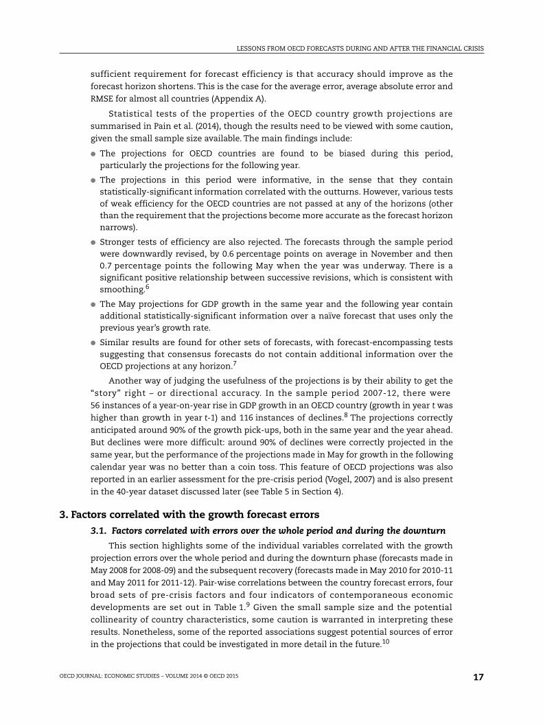
sufficient requirement for forecast efficiency is that accuracy should improve as the
forecast horizon shortens. This is the case for the average error, average absolute error and
RMSE for almost all countries (Appendix A).
Statistical tests of the properties of the OECD country growth projections are
summarised in Pain et al. (2014), though the results need to be viewed with some caution,
given the small sample size available. The main findings include:
● The projections for OECD countries are found to be biased during this period,particularly the projections for the following year.
● The projections in this period were informative, in the sense that they containstatistically-significant information correlated with the outturns. However, various testsof weak efficiency for the OECD countries are not passed at any of the horizons (otherthan the requirement that the projections become more accurate as the forecast horizonnarrows).
● Stronger tests of efficiency are also rejected. The forecasts through the sample periodwere downwardly revised, by 0.6 percentage points on average in November and then0.7 percentage points the following May when the year was underway. There is asignificant positive relationship between successive revisions, which is consistent withsmoothing.6
● The May projections for GDP growth in the same year and the following year containadditional statistically-significant information over a naïve forecast that uses only theprevious year’s growth rate.
● Similar results are found for other sets of forecasts, with forecast-encompassing testssuggesting that consensus forecasts do not contain additional information over theOECD projections at any horizon.7
Another way of judging the usefulness of the projections is by their ability to get the
“story” right – or directional accuracy. In the sample period 2007-12, there were
56 instances of a year-on-year rise in GDP growth in an OECD country (growth in year t was
higher than growth in year t-1) and 116 instances of declines.8 The projections correctly
anticipated around 90% of the growth pick-ups, both in the same year and the year ahead.
But declines were more difficult: around 90% of declines were correctly projected in the
same year, but the performance of the projections made in May for growth in the following
calendar year was no better than a coin toss. This feature of OECD projections was also
reported in an earlier assessment for the pre-crisis period (Vogel, 2007) and is also present
in the 40-year dataset discussed later (see Table 5 in Section 4).
3. Factors correlated with the growth forecast errors
3.1. Factors correlated with errors over the whole period and during the downturn
This section highlights some of the individual variables correlated with the growth
projection errors over the whole period and during the downturn phase (forecasts made in
May 2008 for 2008-09) and the subsequent recovery (forecasts made in May 2010 for 2010-11
and May 2011 for 2011-12). Pair-wise correlations between the country forecast errors, four
broad sets of pre-crisis factors and four indicators of contemporaneous economic
developments are set out in Table 1.9 Given the small sample size and the potential
collinearity of country characteristics, some caution is warranted in interpreting these
results. Nonetheless, some of the reported associations suggest potential sources of error
in the projections that could be investigated in more detail in the future.10
LESSONS FROM OECD FORECASTS DURING AND AFTER THE FINANCIAL CRISIS
OECD JOURNAL: ECONOMIC STUDIES – VOLUME 2014 © OECD 201518
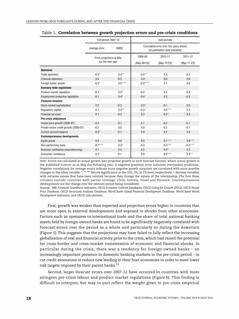
First, growth was weaker than expected and projection errors higher in countries that
are more open to external developments and exposed to shocks from other economies.
Factors such as openness to international trade and the share of total national banking
assets held by foreign-owned banks are found to be significantly negatively correlated with
forecast errors over the period as a whole and particularly so during the downturn
(Figure 5). This suggests that the projections may have failed to fully reflect the increasing
globalisation of real and financial activity prior to the crisis, which had raised the potential
for cross-border and cross-market transmission of economic and financial shocks. In
particular during the crisis, there was a tendency for foreign-owned banks – an
increasingly important presence in domestic banking markets in the pre-crisis period – to
cut credit extensions or reduce new lending in their host economies in order to meet lower
risk targets imposed by their parent banks.11
Second, larger forecast errors over 2007-12 have occurred in countries with more
stringent pre-crisis labour and product market regulations (Figure 6). This finding is
difficult to interpret, but may in part reflect the weight given to pre-crisis empirical
Table 1. Correlation between growth projection errors and pre-crisis conditions
Full period: 2007-12 Sub-periods
Average error RMSECumulative error over two years shown
(at publication date indicated)
From projections at Mayfor the next year
2008-09 2010-11 2011-12
(May-08 EO) (May-10 EO) (May-11 EO)
Openness
Trade openness -0.3* 0.4** -0.4** 0.0 -0.3
Financial openness^ 0.3 -0.3 0.4* 0.0 0.0
Foreign banks' assets -0.3* 0.5*** -0.5*** 0.1 0.0
Economy-wide regulations
Product market regulation -0.1 0.3* -0.2 0.2 -0.2
Employment protection legislation -0.1 0.4* -0.4* 0.3 -0.2
Financial structure
Stock market capitalisation 0.2 -0.3 0.3* -0.1 0.0
Regulatory capital 0.1 0.4** -0.3* 0.5*** 0.3
Financial services^ 0.1 -0.3 0.3 -0.3* 0.3
Pre-crisis imbalances
House price growth (2000-07) -0.2 -0.1 0.1 -0.2 -0.1
Private-sector credit growth (2000-07) -0.2 0.0 0.0 -0.2 -0.1
Current account balance 0.3* -0.1 0.0 0.2 0.0
Contemporaneous developments
Equity prices 0.3 0.0 0.0 0.7*** 0.8***
Non-performing loans -0.7*** 0.3* -0.3 -0.5*** -0.5***
Business confidence (manufacturing) 0.1 0.0 0.2 0.4* 0.2
Consumer confidence 0.3* -0.1 0.0 0.6*** 0.4**
Note: Errors are calculated as actual growth less projected growth at each forecast horizon, where actual growth isthe published outturn as at May the following year. A negative (positive) error indicates over(under)-prediction.Negative correlations for average errors indicate more negative growth surprises are correlated with more positivechanges in the other variable. *, **, *** denote significance at the 10%, 5%, or 1% level, respectively. ^ denotes variableswith extreme values that have been omitted because they change the nature of the relationship. The first threecolumns exclude countries with partial coverage: Chile, Estonia, Israel and Slovenia. Contemporaneousdevelopments are the change over the relevant period being considered.Sources: IMF, Financial Soundness Indicators, OECD Economic Outlook Databases; OECD Going for Growth (2012); OECD HousePrice Database; OECD Structural Analysis Database; World Bank Global Financial Development Database; World Bank WorldDevelopment Indicators; and OECD calculations.
LESSONS FROM OECD FORECASTS DURING AND AFTER THE FINANCIAL CRISIS
OECD JOURNAL: ECONOMIC STUDIES – VOLUME 2014 © OECD 2015 19
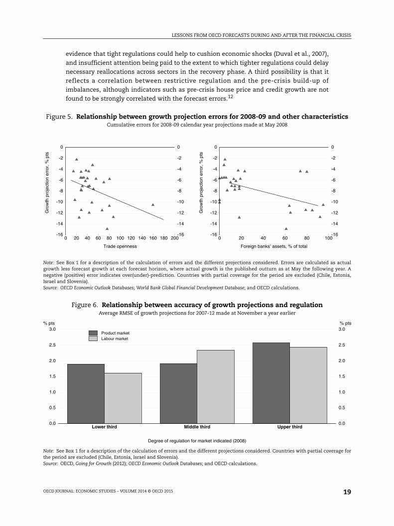
evidence that tight regulations could help to cushion economic shocks (Duval et al., 2007),
and insufficient attention being paid to the extent to which tighter regulations could delay
necessary reallocations across sectors in the recovery phase. A third possibility is that it
reflects a correlation between restrictive regulation and the pre-crisis build-up of
imbalances, although indicators such as pre-crisis house price and credit growth are not
found to be strongly correlated with the forecast errors.12
Figure 5. Relationship between growth projection errors for 2008-09 and other characteristicsCumulative errors for 2008-09 calendar year projections made at May 2008
Note: See Box 1 for a description of the calculation of errors and the different projections considered. Errors are calculated as actualgrowth less forecast growth at each forecast horizon, where actual growth is the published outturn as at May the following year. Anegative (positive) error indicates over(under)-prediction. Countries with partial coverage for the period are excluded (Chile, Estonia,Israel and Slovenia).Source: OECD Economic Outlook Databases; World Bank Global Financial Development Database; and OECD calculations.
Figure 6. Relationship between accuracy of growth projections and regulationAverage RMSE of growth projections for 2007-12 made at November a year earlier
Note: See Box 1 for a description of the calculation of errors and the different projections considered. Countries with partial coverage forthe period are excluded (Chile, Estonia, Israel and Slovenia).Source: OECD, Going for Growth (2012); OECD Economic Outlook Databases; and OECD calculations.
0 20 40 60 80 100 120 140 160 180 200-16
-14
-12
-10
-8
-6
-4
-2
0
-16
-14
-12
-10
-8
-6
-4
-2
0
Gro
wth
pro
ject
ion
erro
r, %
pts
Trade openness
0 20 40 60 80 100-16
-14
-12
-10
-8
-6
-4
-2
0
-16
-14
-12
-10
-8
-6
-4
-2
0
Gro
wth
pro
ject
ion
erro
r, %
pts
Foreign banks’ assets, % of total
Lower third Middle third Upper third0.0
0.5
1.0
1.5
2.0
2.5
3.0% pts
0.0
0.5
1.0
1.5
2.0
2.5
3.0% pts
Product marketLabour market
Degree of regulation for market indicated (2008)
LESSONS FROM OECD FORECASTS DURING AND AFTER THE FINANCIAL CRISIS
OECD JOURNAL: ECONOMIC STUDIES – VOLUME 2014 © OECD 201520
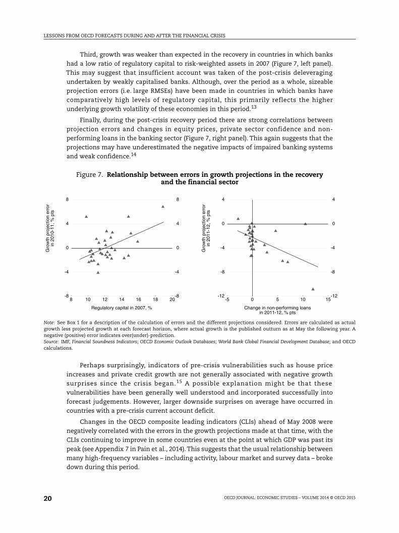
Third, growth was weaker than expected in the recovery in countries in which banks
had a low ratio of regulatory capital to risk-weighted assets in 2007 (Figure 7, left panel).
This may suggest that insufficient account was taken of the post-crisis deleveraging
undertaken by weakly capitalised banks. Although, over the period as a whole, sizeable
projection errors (i.e. large RMSEs) have been made in countries in which banks have
comparatively high levels of regulatory capital, this primarily reflects the higher
underlying growth volatility of these economies in this period.13
Finally, during the post-crisis recovery period there are strong correlations between
projection errors and changes in equity prices, private sector confidence and non-
performing loans in the banking sector (Figure 7, right panel). This again suggests that the
projections may have underestimated the negative impacts of impaired banking systems
and weak confidence.14
Perhaps surprisingly, indicators of pre-crisis vulnerabilities such as house price
increases and private credit growth are not generally associated with negative growth
surprises since the crisis began.15 A possible explanation might be that these
vulnerabilities have been generally well understood and incorporated successfully into
forecast judgements. However, larger downside surprises on average have occurred in
countries with a pre-crisis current account deficit.
Changes in the OECD composite leading indicators (CLIs) ahead of May 2008 were
negatively correlated with the errors in the growth projections made at that time, with the
CLIs continuing to improve in some countries even at the point at which GDP was past its
peak (see Appendix 7 in Pain et al., 2014). This suggests that the usual relationship between
many high-frequency variables – including activity, labour market and survey data – broke
down during this period.
Figure 7. Relationship between errors in growth projections in the recoveryand the financial sector
Note: See Box 1 for a description of the calculation of errors and the different projections considered. Errors are calculated as actualgrowth less projected growth at each forecast horizon, where actual growth is the published outturn as at May the following year. Anegative (positive) error indicates over(under)-prediction.Source: IMF, Financial Soundness Indicators; OECD Economic Outlook Databases; World Bank Global Financial Development Database; and OECDcalculations.
8 10 12 14 16 18 20-8
-4
0
4
8
-8
-4
0
4
8
Gro
wth
pro
ject
ion
erro
rin
201
0-11
, % p
ts
Regulatory capital in 2007, %
-5 0 5 10 15-12
-8
-4
0
4
-12
-8
-4
0
4G
row
th p
roje
ctio
n er
ror
in 2
011-
12, %
pts
Change in non-performing loansin 2011-12, % pts
LESSONS FROM OECD FORECASTS DURING AND AFTER THE FINANCIAL CRISIS
OECD JOURNAL: ECONOMIC STUDIES – VOLUME 2014 © OECD 2015 21
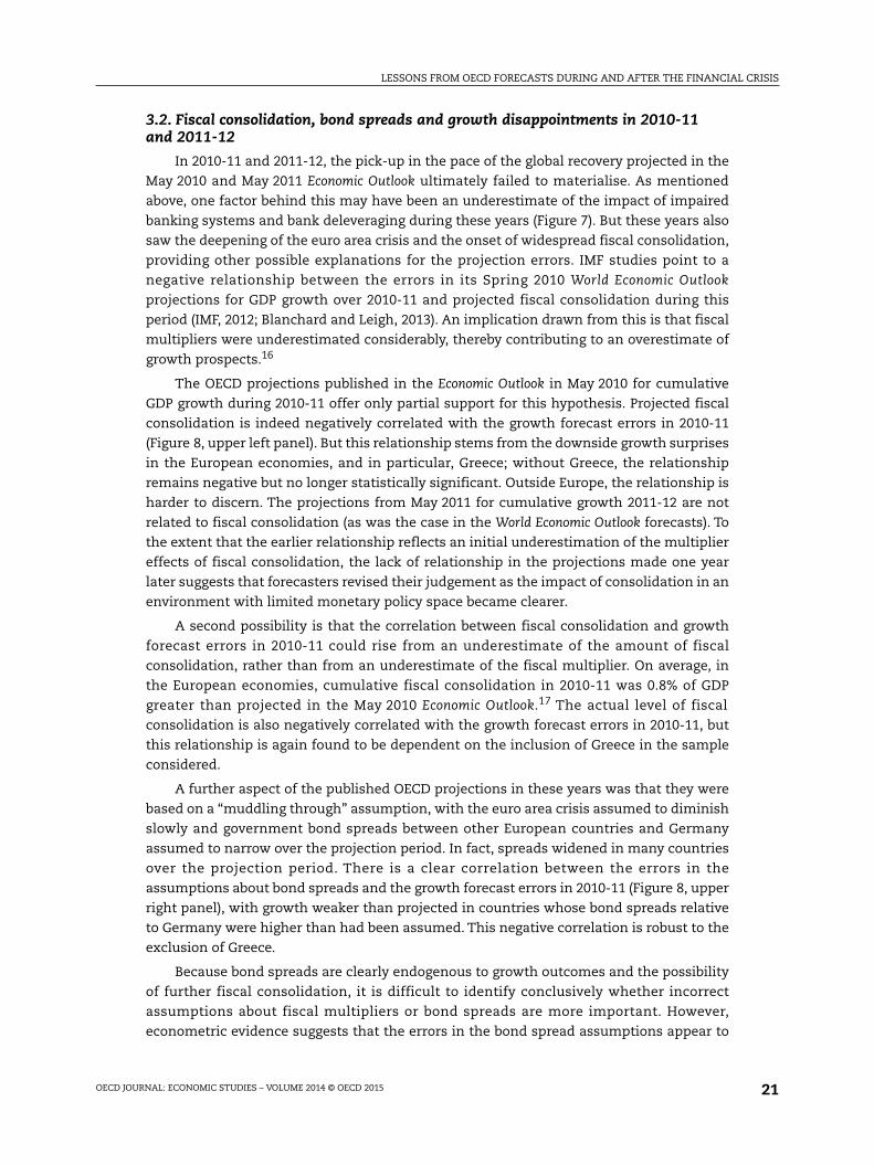
3.2. Fiscal consolidation, bond spreads and growth disappointments in 2010-11and 2011-12
In 2010-11 and 2011-12, the pick-up in the pace of the global recovery projected in the
May 2010 and May 2011 Economic Outlook ultimately failed to materialise. As mentioned
above, one factor behind this may have been an underestimate of the impact of impaired
banking systems and bank deleveraging during these years (Figure 7). But these years also
saw the deepening of the euro area crisis and the onset of widespread fiscal consolidation,
providing other possible explanations for the projection errors. IMF studies point to a
negative relationship between the errors in its Spring 2010 World Economic Outlook
projections for GDP growth over 2010-11 and projected fiscal consolidation during this
period (IMF, 2012; Blanchard and Leigh, 2013). An implication drawn from this is that fiscal
multipliers were underestimated considerably, thereby contributing to an overestimate of
growth prospects.16
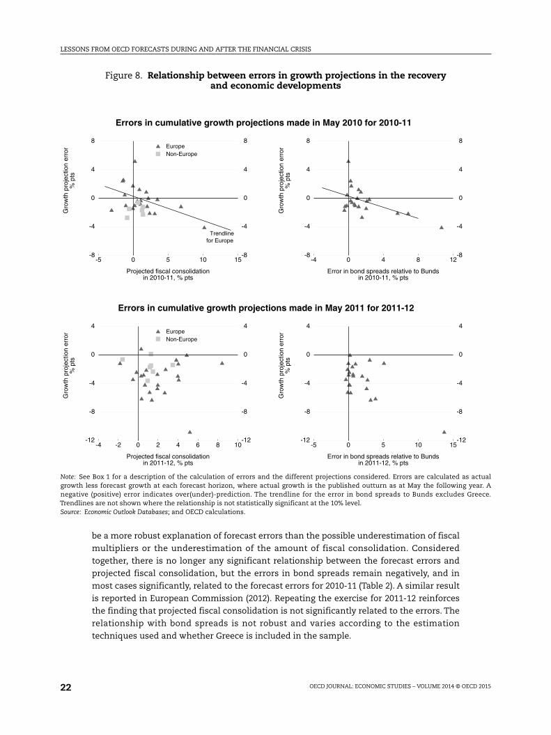
The OECD projections published in the Economic Outlook in May 2010 for cumulative
GDP growth during 2010-11 offer only partial support for this hypothesis. Projected fiscal
consolidation is indeed negatively correlated with the growth forecast errors in 2010-11
(Figure 8, upper left panel). But this relationship stems from the downside growth surprises
in the European economies, and in particular, Greece; without Greece, the relationship
remains negative but no longer statistically significant. Outside Europe, the relationship is
harder to discern. The projections from May 2011 for cumulative growth 2011-12 are not
related to fiscal consolidation (as was the case in the World Economic Outlook forecasts). To
the extent that the earlier relationship reflects an initial underestimation of the multiplier
effects of fiscal consolidation, the lack of relationship in the projections made one year
later suggests that forecasters revised their judgement as the impact of consolidation in an
environment with limited monetary policy space became clearer.
A second possibility is that the correlation between fiscal consolidation and growth
forecast errors in 2010-11 could rise from an underestimate of the amount of fiscal
consolidation, rather than from an underestimate of the fiscal multiplier. On average, in
the European economies, cumulative fiscal consolidation in 2010-11 was 0.8% of GDP
greater than projected in the May 2010 Economic Outlook.17 The actual level of fiscal
consolidation is also negatively correlated with the growth forecast errors in 2010-11, but
this relationship is again found to be dependent on the inclusion of Greece in the sample
considered.
A further aspect of the published OECD projections in these years was that they were
based on a “muddling through” assumption, with the euro area crisis assumed to diminish
slowly and government bond spreads between other European countries and Germany
assumed to narrow over the projection period. In fact, spreads widened in many countries
over the projection period. There is a clear correlation between the errors in the
assumptions about bond spreads and the growth forecast errors in 2010-11 (Figure 8, upper
right panel), with growth weaker than projected in countries whose bond spreads relative
to Germany were higher than had been assumed. This negative correlation is robust to the
exclusion of Greece.
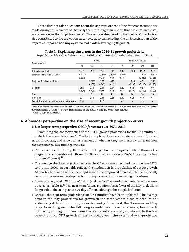
Because bond spreads are clearly endogenous to growth outcomes and the possibility
of further fiscal consolidation, it is difficult to identify conclusively whether incorrect
assumptions about fiscal multipliers or bond spreads are more important. However,
econometric evidence suggests that the errors in the bond spread assumptions appear to
LESSONS FROM OECD FORECASTS DURING AND AFTER THE FINANCIAL CRISIS
OECD JOURNAL: ECONOMIC STUDIES – VOLUME 2014 © OECD 201522
be a more robust explanation of forecast errors than the possible underestimation of fiscal
multipliers or the underestimation of the amount of fiscal consolidation. Considered
together, there is no longer any significant relationship between the forecast errors and
projected fiscal consolidation, but the errors in bond spreads remain negatively, and in
most cases significantly, related to the forecast errors for 2010-11 (Table 2). A similar result
is reported in European Commission (2012). Repeating the exercise for 2011-12 reinforces
the finding that projected fiscal consolidation is not significantly related to the errors. The
relationship with bond spreads is not robust and varies according to the estimation
techniques used and whether Greece is included in the sample.
Figure 8. Relationship between errors in growth projections in the recoveryand economic developments
Note: See Box 1 for a description of the calculation of errors and the different projections considered. Errors are calculated as actualgrowth less forecast growth at each forecast horizon, where actual growth is the published outturn as at May the following year. Anegative (positive) error indicates over(under)-prediction. The trendline for the error in bond spreads to Bunds excludes Greece.Trendlines are not shown where the relationship is not statistically significant at the 10% level.Source: Economic Outlook Databases; and OECD calculations.
-5 0 5 10 15-8
-4
0
4
8
-8
-4
0
4
8
Errors in cumulative growth projections made in May 2010 for 2010-11
Trendlinefor Europe
EuropeNon-Europe
Gro
wth
pro
ject
ion
erro
r%
pts
Projected fiscal consolidationin 2010-11, % pts
-4 0 4 8 12-8
-4
0
4
8
-8
-4
0
4
8
Gro
wth
pro
ject
ion
erro
r%
pts
Error in bond spreads relative to Bundsin 2010-11, % pts
-4 -2 0 2 4 6 8 10-12
-8
-4
0
4
-12
-8
-4
0
4
Errors in cumulative growth projections made in May 2011 for 2011-12
EuropeNon-Europe
Gro
wth
pro
ject
ion
erro
r%
pts
Projected fiscal consolidationin 2011-12, % pts
-5 0 5 10 15-12
-8
-4
0
4
-12
-8
-4
0
4
Gro
wth
pro
ject
ion
erro
r%
pts
Error in bond spreads relative to Bundsin 2011-12, % pts
LESSONS FROM OECD FORECASTS DURING AND AFTER THE FINANCIAL CRISIS
OECD JOURNAL: ECONOMIC STUDIES – VOLUME 2014 © OECD 2015 23
These findings raise questions about the appropriateness of the forecast assumptions
made during the recovery, particularly the prevailing assumption that the euro area crisis
would ease over the projection period. This issue is discussed further below. Other factors
also contributed to the projection errors over 2010-12, including the underestimation of the
impact of impaired banking systems and bank deleveraging (Figure 7).
4. A broader perspective on the size of recent growth projection errors
4.1. A longer-term perspective: OECD forecasts over 1971-2012
Examining the characteristics of the OECD growth projections for the G7 countries –
for which there are data from 1971 – helps to place the characteristics of recent forecast
errors in context, and allows an assessment of whether they are markedly different from
past experience. Key findings include:
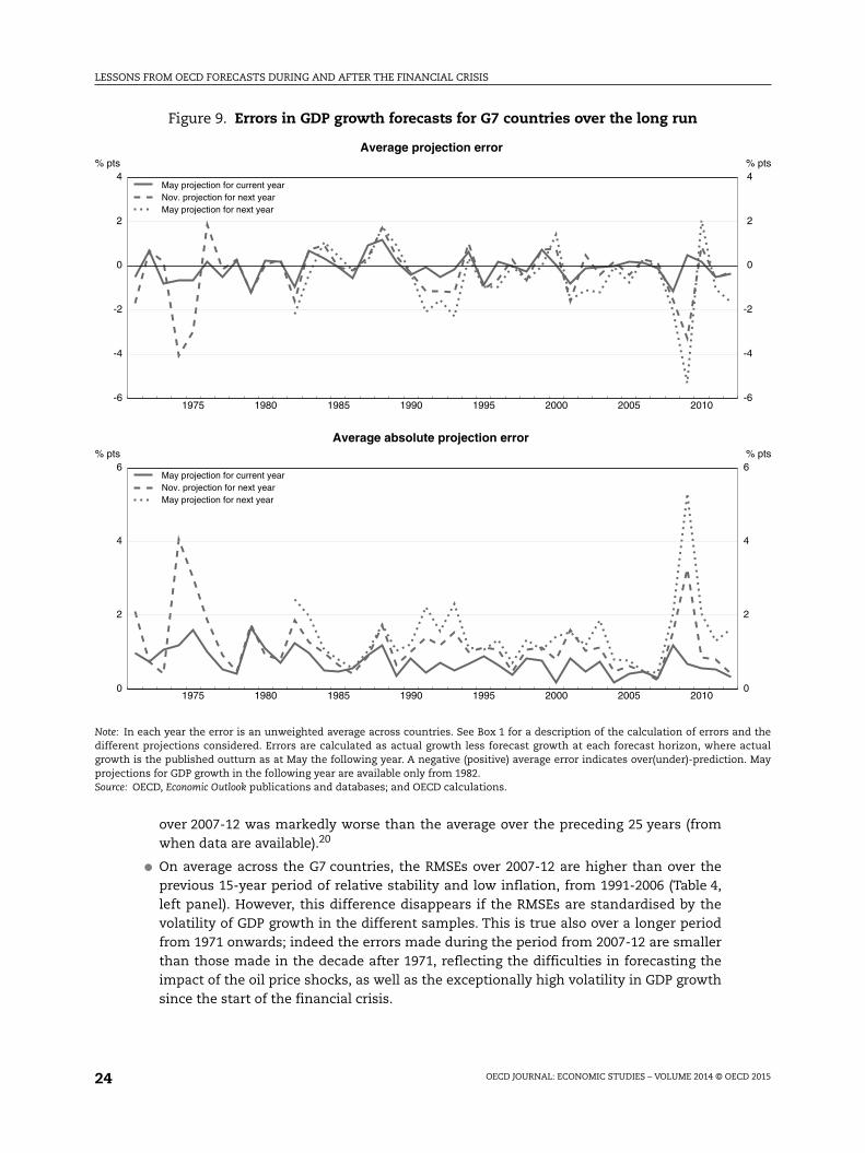
● The errors made during the crisis are large, but not unprecedented. Errors of amagnitude comparable with those in 2009 occurred in the early 1970s, following the firstoil crisis (Figure 9).18
● The average absolute projection error in the G7 economies declined from the late 1970s
to the mid-2000s. In part, this reflects the moderation in the volatility of output growth.
At shorter horizons the decline might also reflect improved data availability, especially
regarding near-term developments, and improvements in forecasting procedures.
● In many cases, weak efficiency of the projections for G7 countries over four decades cannotbe rejected (Table 3).19 The near-term forecasts perform best; fewer of the May projectionsfor growth in the next year are weakly efficient, although the sample is shorter.
● Overall, the near-term projections for G7 countries have been unbiased. The averageerror in the May projections for growth in the same year is close to zero (or notstatistically different from zero) for each country. In contrast, the November and Mayprojections for growth the following calendar year have, on average, been overlyoptimistic, although in many cases the bias is not statistically significant. In the Mayprojections for GDP growth in the following year, the extent of over-prediction
Table 2. Explaining the errors in the 2010-11 growth projectionsDependent variable: Cumulative error in the GDP growth projections made in May 2010 for 2010-11
Country sampleEurope Europe excl. Greece
(1) (2) (3) (4) (5) (6) (7) (8)
Estimation method TSLS OLS TSLS OLS TSLS OLS TSLS OLS
Error in bond spreads (to Bunds) -0.43***(0.087)
-0.47**(0.210)
-0.36***(0.126)
-0.44**(0.181)
-0.49*(0.243)
-0.36**(0.135)
Projected fiscal consolidation -0.31**(0.136)
0.02(0.207)
-0.05(0.155)
-0.19(0.168)
0.01(0.213)
-0.05(0.193)
Constant 0.52(0.484)
0.22(0.488)
0.54(0.508)
0.47(0.482)
0.52(0.563)
0.16(0.499)
0.57(0.599)
0.46(0.553)
Obs 21 21 21 21 20 20 20 20
R-squared 0.34 0.22 0.34 0.34 0.17 0.05 0.16 0.17
F-statistic of excluded instruments from first stage 61.0 - 21.7 - 16.1 - 12.9 -
Note: The sample is restricted to those countries with values for both variables. Robust standard errors are reportedin parenthesis. *, **, and *** denote significance at the 10%, 5% and 1% levels, respectively.Source: OECD calculations.
LESSONS FROM OECD FORECASTS DURING AND AFTER THE FINANCIAL CRISIS
OECD JOURNAL: ECONOMIC STUDIES – VOLUME 2014 © OECD 201524
over 2007-12 was markedly worse than the average over the preceding 25 years (fromwhen data are available).20
● On average across the G7 countries, the RMSEs over 2007-12 are higher than over theprevious 15-year period of relative stability and low inflation, from 1991-2006 (Table 4,left panel). However, this difference disappears if the RMSEs are standardised by thevolatility of GDP growth in the different samples. This is true also over a longer periodfrom 1971 onwards; indeed the errors made during the period from 2007-12 are smallerthan those made in the decade after 1971, reflecting the difficulties in forecasting theimpact of the oil price shocks, as well as the exceptionally high volatility in GDP growthsince the start of the financial crisis.
Figure 9. Errors in GDP growth forecasts for G7 countries over the long run
Note: In each year the error is an unweighted average across countries. See Box 1 for a description of the calculation of errors and thedifferent projections considered. Errors are calculated as actual growth less forecast growth at each forecast horizon, where actualgrowth is the published outturn as at May the following year. A negative (positive) average error indicates over(under)-prediction. Mayprojections for GDP growth in the following year are available only from 1982.Source: OECD, Economic Outlook publications and databases; and OECD calculations.
1975 1980 1985 1990 1995 2000 2005 2010-6
-4
-2
0
2
4% pts
-6
-4
-2
0
2
4% pts
May projection for current yearNov. projection for next yearMay projection for next year
Average projection error
1975 1980 1985 1990 1995 2000 2005 20100
2
4
6% pts
0
2
4
6% pts
May projection for current yearNov. projection for next yearMay projection for next year
Average absolute projection error
LESSONS FROM OECD FORECASTS DURING AND AFTER THE FINANCIAL CRISIS
OECD JOURNAL: ECONOMIC STUDIES – VOLUME 2014 © OECD 2015 25
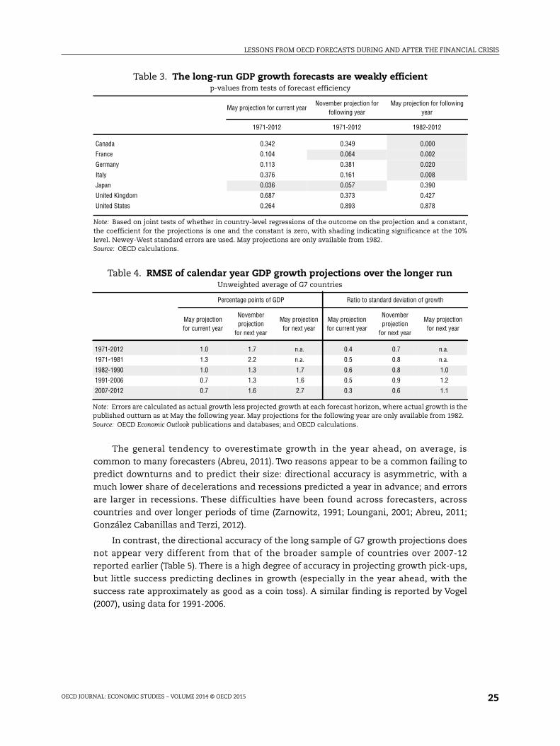
The general tendency to overestimate growth in the year ahead, on average, is
common to many forecasters (Abreu, 2011). Two reasons appear to be a common failing to
predict downturns and to predict their size: directional accuracy is asymmetric, with a
much lower share of decelerations and recessions predicted a year in advance; and errors
are larger in recessions. These difficulties have been found across forecasters, across
countries and over longer periods of time (Zarnowitz, 1991; Loungani, 2001; Abreu, 2011;
González Cabanillas and Terzi, 2012).
In contrast, the directional accuracy of the long sample of G7 growth projections does
not appear very different from that of the broader sample of countries over 2007-12
reported earlier (Table 5). There is a high degree of accuracy in projecting growth pick-ups,
but little success predicting declines in growth (especially in the year ahead, with the
success rate approximately as good as a coin toss). A similar finding is reported by Vogel
(2007), using data for 1991-2006.
Table 3. The long-run GDP growth forecasts are weakly efficientp-values from tests of forecast efficiency
May projection for current yearNovember projection for
following yearMay projection for following
year
1971-2012 1971-2012 1982-2012
Canada 0.342 0.349 0.000
France 0.104 0.064 0.002
Germany 0.113 0.381 0.020
Italy 0.376 0.161 0.008
Japan 0.036 0.057 0.390
United Kingdom 0.687 0.373 0.427
United States 0.264 0.893 0.878
Note: Based on joint tests of whether in country-level regressions of the outcome on the projection and a constant,the coefficient for the projections is one and the constant is zero, with shading indicating significance at the 10%level. Newey-West standard errors are used. May projections are only available from 1982.Source: OECD calculations.
Table 4. RMSE of calendar year GDP growth projections over the longer runUnweighted average of G7 countries
Percentage points of GDP Ratio to standard deviation of growth
May projectionfor current year
Novemberprojection
for next year
May projectionfor next year
May projectionfor current year
Novemberprojection
for next year
May projectionfor next year
1971-2012 1.0 1.7 n.a. 0.4 0.7 n.a.
1971-1981 1.3 2.2 n.a. 0.5 0.8 n.a.
1982-1990 1.0 1.3 1.7 0.6 0.8 1.0
1991-2006 0.7 1.3 1.6 0.5 0.9 1.2
2007-2012 0.7 1.6 2.7 0.3 0.6 1.1
Note: Errors are calculated as actual growth less projected growth at each forecast horizon, where actual growth is thepublished outturn as at May the following year. May projections for the following year are only available from 1982.Source: OECD Economic Outlook publications and databases; and OECD calculations.
LESSONS FROM OECD FORECASTS DURING AND AFTER THE FINANCIAL CRISIS
OECD JOURNAL: ECONOMIC STUDIES – VOLUME 2014 © OECD 201526
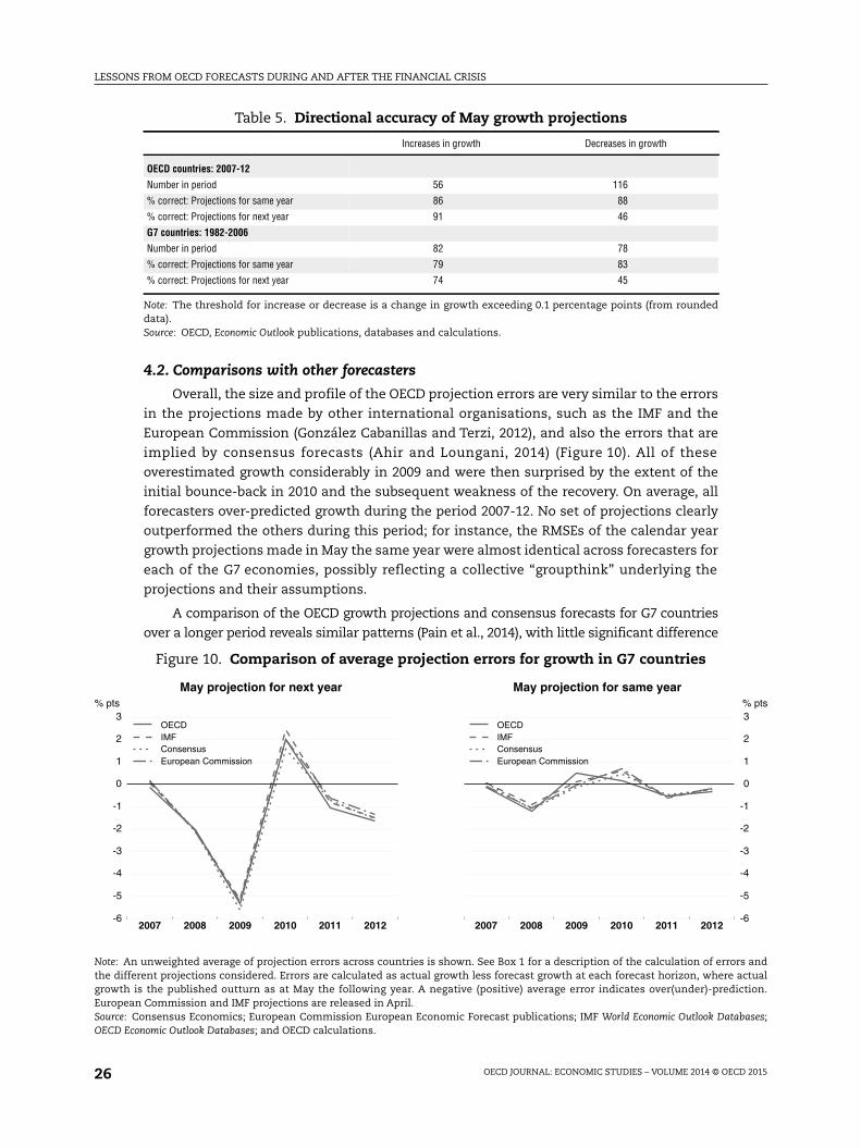
4.2. Comparisons with other forecasters
Overall, the size and profile of the OECD projection errors are very similar to the errors
in the projections made by other international organisations, such as the IMF and the
European Commission (González Cabanillas and Terzi, 2012), and also the errors that are
implied by consensus forecasts (Ahir and Loungani, 2014) (Figure 10). All of these
overestimated growth considerably in 2009 and were then surprised by the extent of the
initial bounce-back in 2010 and the subsequent weakness of the recovery. On average, all
forecasters over-predicted growth during the period 2007-12. No set of projections clearly
outperformed the others during this period; for instance, the RMSEs of the calendar year
growth projections made in May the same year were almost identical across forecasters for
each of the G7 economies, possibly reflecting a collective “groupthink” underlying the
projections and their assumptions.
A comparison of the OECD growth projections and consensus forecasts for G7 countries
over a longer period reveals similar patterns (Pain et al., 2014), with little significant difference
Table 5. Directional accuracy of May growth projections
Increases in growth Decreases in growth
OECD countries: 2007-12
Number in period 56 116
% correct: Projections for same year 86 88
% correct: Projections for next year 91 46
G7 countries: 1982-2006
Number in period 82 78
% correct: Projections for same year 79 83
% correct: Projections for next year 74 45
Note: The threshold for increase or decrease is a change in growth exceeding 0.1 percentage points (from roundeddata).Source: OECD, Economic Outlook publications, databases and calculations.
Figure 10. Comparison of average projection errors for growth in G7 countries
Note: An unweighted average of projection errors across countries is shown. See Box 1 for a description of the calculation of errors andthe different projections considered. Errors are calculated as actual growth less forecast growth at each forecast horizon, where actualgrowth is the published outturn as at May the following year. A negative (positive) average error indicates over(under)-prediction.European Commission and IMF projections are released in April.Source: Consensus Economics; European Commission European Economic Forecast publications; IMF World Economic Outlook Databases;OECD Economic Outlook Databases; and OECD calculations.
2007 2008 2009 2010 2011 2012-6
-5
-4
-3
-2
-1
0
1
2
3% pts
OECDIMFConsensusEuropean Commission
May projection for next year
2007 2008 2009 2010 2011 2012
-6
-5
-4
-3
-2
-1
0
1
2
3% pts
OECDIMFConsensusEuropean Commission
May projection for same year
LESSONS FROM OECD FORECASTS DURING AND AFTER THE FINANCIAL CRISIS
OECD JOURNAL: ECONOMIC STUDIES – VOLUME 2014 © OECD 2015 27
in the overall accuracy of the OECD and consensus forecasts over the past two decades.
Forecast-encompassing tests (Fair and Shiller, 1990) suggest that the OECD May current-year
projections and November year-ahead projections encompass the consensus forecasts
(i.e. contain all the relevant information found in the consensus forecasts). However, neither of
the separate May projections for growth in the following year encompasses the other. This is
the case for both the pre-crisis period and also over 2007-2012.
4.3. The nature of the projections
The OECD forecasts are conditional projections rather than pure forecasts. The
projections are consistent with the advice given about monetary policy settings and rest on
explicit and implicit assumptions, such as fiscal policy changes and whether the euro area
crisis will be successfully contained. Some potentially endogenous factors, such as
commodity prices and nominal exchange rates, are also switched off over the projection
period.21 This raises a number of difficult issues.
One issue is that the projections, and especially the accompanying commentary,
sometimes point to unsustainable developments and the need for policy changes. If these
are built into the projections, but the advice is not followed (or vice versa), an error in the
projections will likely occur. It is not clear how or whether this type of error can be
controlled for in the projection process.
A related issue, as noted above, is that the projections made during the euro area crisis
placed a lot of weight on the assumption that the euro area crisis would be contained and
subsequently ease, with accompanying declines in sovereign bond spreads and improvements
in confidence. Yet it is not clear what else could have been assumed in projections for a period
of over two years made public by an inter-governmental organisation. One possible answer –
and the route chosen by the OECD at the time – is to make extensive use of scenario analyses
to quantify possible adverse outcomes if key assumptions did not hold.
A third issue relates to the interpretation of the forecasts since the onset of the crisis.
Given the skewed distribution of possible projections, depending on the assumptions
chosen, and the emergence of fat negative tail risks, the nature of the published projections
has changed. Whereas previously they were best seen as mean projections, more recently
they have become modal forecasts, i.e. reflecting the most likely outcome. This has,
however, resulted in a communications problem, as many users of the projections still
view them as mean projections with a balanced distribution of risks.
5. Recent changes in forecasting techniques and proceduresand the unfinished agenda
The challenges encountered in forecasting in recent years have led to changes in
forecasting techniques and procedures in the OECD and in other international
organisations, some of them still in progress. Key developments are outlined below,
drawing on OECD experience and consultations with experts from the IMF, World Bank,
European Commission and European Central Bank.22
5.1. Increases in the centralisation or “top-down” component of the forecast process
Reflecting the common errors made in all country forecasts in recent years, and the
extent to which these have been associated with stronger than expected global financial,
LESSONS FROM OECD FORECASTS DURING AND AFTER THE FINANCIAL CRISIS
OECD JOURNAL: ECONOMIC STUDIES – VOLUME 2014 © OECD 201528
trade and sentiment interconnections, increasing weight has been placed on central
strategic guidance at an early stage of the forecast process, at the OECD and elsewhere.
● One aspect has been early identification of key global developments and risks and theirlikely quantitative implications for global activity and global trade. This ensures aconsistent view amongst country specialists of forces acting on the forecasts andoutlook for the major economies.
● Initial early guidance in the form of top-down centralised projections is now provided atthe OECD and elsewhere, to help ensure that projections for individual countries arebased on a common general storyline. These projections draw together the key pointsfrom standalone analyses such as indicator models and assessments of financial marketdevelopments.
5.2. Enhanced monitoring of near-term activity developments
Although it took time for the full effects of the sub-prime and Lehman Brothers
collapse to start to appear in published activity data, they were reflected swiftly in high-
frequency tendency surveys. Developments such as the generalised collapse of confidence
during the Great Recession and more recently when the euro area crisis intensified have
also pointed to the potential usefulness of early survey-based signals. This has been
reflected in a number of ongoing developments:
● The longstanding use of statistical composite leading indicators by the OECD has beenaugmented by the use of empirical “nowcasting” models, exploiting high-frequencyinformation to gain an early picture of key activity developments (Box 2). Examples usedby the OECD in forming projections for the Economic Outlook include the suite of quarterlyGDP growth models for G7 economies introduced a decade ago (Sédillot and Pain, 2003),and the more recently-developed suite of indicator models for global trade (Guichardand Rusticelli, 2011). The OECD growth indicator models during the crisis provided a veryuseful real-time signal of a significant slowdown and then major contraction. Elsewhere,the indicator model approach is being extended by using high-frequency information tomodel private sector expenditure. Assessments are also being undertaken of possiblenon-linearities in the relationship between indicator variables and growth outcomes attimes of extreme stress.
● Greater use has also been made of the anecdotal information gathered from outsidebusiness contacts. At times of fast-moving financial developments these may provide anearly signal of changes in factors such as credit conditions, and thus near-term activitydevelopments. One example given in the interviews was an early signal about theimpact of a freezing of trade credits at the height of the crisis.
● Increasing attempts have been made, though not yet in the OECD, to utilise high-frequency information on real-time activity developments provided by internet-basedindicators (“big data”). Internet-based search measures, based on Google Trends, havebeen used to identify early signals about specific housing and labour marketdevelopments (Hellerstein and Middeldorp, 2012; McLaren and Shanbhogue, 2011), aswell as policy uncertainty (Baker et al., 2012). Recent studies have also sought to use real-time financial transactions data (such as the volume of SWIFT banking transactions, ordata on credit card transactions) as an early indicator of GDP growth and trends in globaltrade finance (Gill et al., 2012).23 The usefulness of such indicators when combined withother longstanding indicator variables has yet to be explored.
LESSONS FROM OECD FORECASTS DURING AND AFTER THE FINANCIAL CRISIS
OECD JOURNAL: ECONOMIC STUDIES – VOLUME 2014 © OECD 2015 29
Box 2. Indicator models, composite leading indicators and OECD projections
Two models available to OECD forecasters are the short-term indicator models, which are used to predictGDP growth for two quarters, and the OECD Composite Leading Indicators (CLIs), which are designed topredict turning points in growth relative to trend. As explained below, both tools are designed to extractinformation about growth from high frequency and timely data sources. By responding reasonably rapidly,the reliance on the indicator models likely reduced overall forecast errors. But it does seem that better useof the information in the CLIs could have reduced the forecast errors in the November projections forgrowth in the following year (but not the other horizons).
Although both tools combine recent data to produce signals about economic growth, they are different byconstruction.
● The short-term indicator models (Sédillot and Pain, 2003 and Mourougane, 2006) are regression-basedmodels that efficiently combine available monthly and quarterly data to predict current quarter andquarter-ahead GDP growth for the G7 countries and the euro area. The input data include “hard” data,such as industrial production and retail sales, and “soft” data, such as business and consumersentiment. Because the dependent variable is GDP growth, the process of producing a forecast isstraightforward. Other work has shown the main gain from the indicator approach is for current-quarterforecasts, where estimated indicator models appear to outperform autoregressive time series models,both in terms of size of error and directional accuracy.
● The OECD CLIs are long-running series produced for all OECD countries and some non-OECD countries.For each country, 5-10 series are used that best predict turning points in the business cycle. The CLI istypically available with a two-month lag. Because the results are primarily qualitative, it is possible thatthe information contained in these series is not used optimally in the forecasting round.
The performance of the indicator models in the crisis
The OECD growth indicator models during the crisis provided a very useful real-time signal of asignificant slowdown and then major contraction (see figure below). Nonetheless, large errors wererecorded in the fourth quarter 2008 and early 2009 and even when the third quarter 2008 was underway, thecontraction in growth was not foreseen. But both the downturn and bounce-back were highlightedrelatively quickly. Overall, the indicator models were useful in compiling the projections at that time andlikely reduced the size of the overall errors made.
The real-time performance of the indicator models during the crisis can also be assessed relative to thatin the pre-crisis period and the simulated out-of-sample performance when the models were firstdeveloped. The root mean squared errors (RMSE) for the G7 countries are shown below (see table). There areslight differences in the timing and information sets for each forecast, but in almost all cases one to twomonths of hard indicator data and two to three months of survey data were available for each economy.Four main points emerge from the 2007-12 period:
● The current quarter real-time forecast errors are comparable with those before the crisis (Sédillot andPain, 2005), both in terms of the cross-country pattern of the errors and the size of the errors. A notableexception is the United Kingdom, where the real-time errors since 2007 have been more than doublethose in the pre-crisis period. The errors were also larger in Japan. But overall, the data suggest that thecurrent quarter models have remained a useful guide to current economic activity.
● The real-time forecast errors in the quarter-ahead forecasts were generally larger than might have beenexpected based on those from the pre-crisis period and the initial out-of-sample exercise, particularly inJapan, Germany and the United Kingdom. However, the cross-country differences in the magnitude ofthe errors are broadly comparable with the pre-crisis period. The generally-higher real-time errors over2007-12 appear to be largely due to the relatively greater volatility of growth outcomes in the recentperiod: when the RMSEs are scaled by the standard deviation of growth outcomes, the errors over 2007-12are all smaller, except for the United Kingdom.
LESSONS FROM OECD FORECASTS DURING AND AFTER THE FINANCIAL CRISIS
OECD JOURNAL: ECONOMIC STUDIES – VOLUME 2014 © OECD 201530
Box 2. Indicator models, composite leading indicators and OECD projections (cont.)
● In all economies the real-time errors for the one-quarter ahead forecasts have been greater than thosefor the current quarter forecasts. The difference between the two is smallest for France.
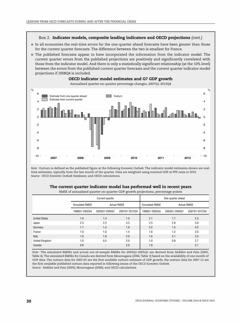
● The published forecasts appear to have incorporated the information from the indicator model. Thecurrent quarter errors from the published projections are positively and significantly correlated withthose from the indicator model. And there is only a statistically significant relationship (at the 10% level)between the errors from the published current quarter forecasts and the current quarter indicator modelprojections if 2008Q4 is included.
OECD indicator model estimates and G7 GDP growthAnnualised quarter-on-quarter percentage changes, 2007Q1-2012Q4
Note: Outturn is defined as the published figure at the following Economic Outlook. The indicator model estimates shown are real-time estimates, typically from the last month of the quarter. Data are weighted using nominal GDP at PPP rates in 2010.Source: OECD Economic Outlook Databases; and OECD calculations.
2007 2008 2009 2010 2011 2012-10
-8
-6
-4
-2
0
2
4
6%
-10
-8
-6
-4
-2
0
2
4
6%
Estimate from one quarter aheadEstimate from current quarter
Outturn
The current quarter indicator model has performed well in recent yearsRMSE of annualised quarter-on-quarter GDP growth projections, percentage points
Current quarter One-quarter ahead
Simulated RMSE Actual RMSE Simulated RMSE Actual RMSE
1998Q1-2002Q4 2003Q1-2005Q1 2007Q1-2012Q4 1998Q1-2002Q4 2003Q1-2005Q1 2007Q1-2012Q4
United States 1.6 1.4 1.5 2.1 1.7 2.3
Japan 2.3 2.3 4.3 2.5 2.8 5.9
Germany 1.7 1.3 1.9 2.2 1.5 4.2
France 1.0 1.0 1.4 1.6 1.2 2.0
Italy 1.0 1.8 2.0 1.6 2.1 3.3
United Kingdom 1.0 0.5 2.0 1.0 0.9 2.7
Canada 0.8 - 2.0 1.8 - 2.7
Note: The simulated RMSEs and actual out-of-sample RMSEs for 2003Q1-2005Q1 are derived from Sédillot and Pain (2005,Table 4). The simulated RMSEs for Canada are derived from Mourougane (2006, Table 3) based on the availability of one month ofGDP data. The outturn data for 2003-05 are the first available outturn estimate of GDP growth; the outturn data for 2007-12 arethe first available published outturn data reported in following issues of the OECD Economic Outlook.Source: Sédillot and Pain (2005); Mourougane (2006); and OECD calculations.
LESSONS FROM OECD FORECASTS DURING AND AFTER THE FINANCIAL CRISIS
OECD JOURNAL: ECONOMIC STUDIES – VOLUME 2014 © OECD 2015 31
5.3. Enhanced monitoring of financial market developments and greater integrationinto the forecast process
Increasing attention is now paid to financial market developments in the construction
of the projections and in empirical analysis.
● As the financial crisis progressed, the OECD Secretariat developed new financialconditions indices (FCIs) for the United States, Japan, the euro area and the UnitedKingdom (Guichard and Turner, 2008; Guichard et al., 2009). These weight together awide range of financial variables that have a well-established link with GDP growth 12 to18 months later.24 The FCIs have been used extensively in the forecasting rounds since2008-09 and as a guide to possible GDP effects in scenario analyses.
● A limitation of the aggregate FCIs is that they do not pick up all recent financial marketdevelopments, notably financial fragmentation in the euro area. Thus someorganisations have also sought to directly incorporate country-specific information onbank lending rates and lending conditions in the set of variables being projected.
● In the OECD and elsewhere, discussions with internal financial market specialists and/or outside experts have been strengthened. In the OECD there are regular contactsbetween the Economics Department and the Directorate for Financial and EnterpriseAffairs. Elsewhere, developments include the establishment of new divisions/unitscovering financial market developments and macro-financial linkages and consideringkey risks.
● Work is underway in some institutions on the difficult tasks of augmenting existingmacroeconomic models with more detailed relationships of banking sector behaviourand strengthening linkages to reflect global financial interconnectedness. Themacroeconomic models available at the time of the crisis typically ignored the bankingsystem and failed to account for the possibility of bank capital shortages and creditrationing having an impact on macroeconomic developments. However, incorporatingthe financial sector into macroeconomic models is proving to be a major challenge.
Box 2. Indicator models, composite leading indicators and OECD projections (cont.)
The usefulness of the OECD composite leading indicators since the crisis began
A simple way of assessing whether the real-time CLIs contained information that might have helped toreduce the real-time projection errors is to regress the errors in GDP growth projections on the change inthe CLIs that would have been available to forecasters at the time. One-month, 3-month, 6-month and 12-month changes up to the projection date in the CLIs for the G7 countries were considered for the period2007-12 (see Appendix 7 of Pain et al., 2014).
Some caution is, of course needed in interpreting the results, but the following points emerge from thisexercise:
● It does not appear that there was some information in the CLIs that could have been used to reduce theprojection errors made in May 2008 as the downturn got underway.
● However, in the early stages of the recovery, at a time of considerable uncertainty, the errors in theNovember 2009 and May 2010 growth projections are found to be positively associated with the changesin the CLIs at the time of the forecast.
LESSONS FROM OECD FORECASTS DURING AND AFTER THE FINANCIAL CRISIS
OECD JOURNAL: ECONOMIC STUDIES – VOLUME 2014 © OECD 201532
5.4. Enhanced focus on risk assessments and global spillovers
Reflecting the uncertainty about the basic assumptions underlying the projections and
the speed and depth of cross-country spillovers since the crisis began, there is now an
enhanced focus on risk assessments and global spillovers in all international organisations:
● Greater information is now being provided about the distribution of risks around thecentral projections. At the OECD, while not providing a numerical risk distribution, therisk profile for the Economic Outlook projections has typically been characterisedqualitatively as being balanced or skewed or bimodal and the projections themselvescharacterised as being modal rather than average projections.25 Other internationalforecasting organisations have presented their assessed numerical risk distribution inthe form of a fan chart or in the form of forecast ranges for key variables.
● Greater use is being made of quantitative scenario analyses to illustrate alternativeoutcomes and their global implications. Two notable examples in the OECD are the scenarioused to illustrate a severe downside outcome arising from adverse euro area developmentsin the latter half of 2011 and the scenario illustrating the impact of the US debt ceilingbecoming binding in the November 2013 Economic Outlook. The first of these scenarios madeuse of new forecasting tools, such as the financial conditions indices and models linkinguncertainty and confidence with final expenditure, as well as a standard macroeconomicmodel, to calibrate the potential near-term activity impact of deteriorating financialconditions and a collapse in confidence brought about by a further worsening of the euroarea crisis. The second used a global macroeconomic model to illustrate the extent to whicha low-probability, but high-impact event would quickly spread to other countries.
Notes
1. The main analysis in this paper is based on calendar year growth rates. Figure 1 uses Q4/Q4 growthrates to illustrate the sudden deterioration in the financial crisis in the last quarter of 2008 and theimpact this had on forecasts at the time.
2. See for example: OECD (2005, 2006), van den Noord (2006), Dieter et al. (2009) and Shigehara andAtkinson (2012).
3. Empirical analysis and macro-model simulations of an increasingly globalised financial systemdid, however, highlight the resulting potential for shocks in one economy to spill over to others toan ever greater extent (Hervé et al., 2007).
4. With the projection errors in each year tending to be in the same direction for almost all countries, theaverage absolute error across countries in Figure 2 is similar in magnitude to the average errors.
5. The projection errors are derived by subtracting the forecast from the outturn, so that anoverestimate of growth results in a negative projection error.
6. This suggests the forecasts are not consistent with full information rational expectations.
7. This is based on the tests of the errors for G7 countries in Appendix 3 of Pain et al. (2014).
8. Changes in growth of less than 0.1 percentage points (from rounded data) are excluded.
9. The set of explanatory variables here is related to that in other studies that seek to explain cross-country differences in growth outcomes during the crisis, including Rose and Spiegel (2010),Cecchetti et al. (2011) and Berkmen et al. (2012). This paper focuses on a smaller set of countries(OECD member countries) and projection errors during the recovery as well as the downturn, andalso considers some contemporaneous developments.
10. Multivariate regressions would better allow causal relationships to be established but are difficultin this small sample. Some preliminary results using the RMSEs of the country growth forecastsare presented in Table A.5.4 of Pain et al. (2014), although caveats still apply. The key finding is thatfor the November year-ahead projection errors, product market regulation remains correlated withaccuracy after controlling for openness, with both variables significant at the 10% level.
LESSONS FROM OECD FORECASTS DURING AND AFTER THE FINANCIAL CRISIS
OECD JOURNAL: ECONOMIC STUDIES – VOLUME 2014 © OECD 2015 33
11. The evidence points to the enhanced exposure of host economies to source economy shocksduring the downturn outweighing the potential for foreign-owned banks, with access to internalcapital resources, to help shield host economies from domestic shocks, which would limit negativegrowth surprises. A related finding is reported by Cetorelli and Goldberg (2012). Claessens and vanHoren (2012) also show that foreign banks reduced their domestic credit more sharply thandomestic banks during the crisis.
12. Related measures of business and labour market regulation produced by the World Bank and theFraser Institute were found to have similar relationships (not shown here).
13. The negative relationship early in the crisis is more difficult to interpret since other studies haveshown that countries with higher capital ratios outperformed those with lower ratios during thattime (Cecchetti et al., 2011). One difference here is the focus on errors, rather than outcomes.Another is the use of regulatory capital (rather than total capital) to risk-weighted assets.
14. It is possible that the correlations could also reflect a reverse causal link, with weaker growthoutcomes leading to more impaired loans and deteriorating confidence. However, qualitativelysimilar results are obtained if confidence changes available at the time of the forecasts are usedinstead.
15. Cecchetti et al. (2011) find that lower pre-crisis levels of private-sector credit to GDP and lowerrates of growth in private-sector credit from 2005-07 were associated with better growth outcomesin the downturn (across a broader sample of countries). In contrast, there is evidence of a positive,but not significant, relationship between the errors in the OECD growth projections and pre-crisislevel of private-sector bank credit.
16. The IMF studies focus primarily on European countries, although the main findings remain even ifthe sample is broadened to other advanced economies.
17. Actual fiscal consolidation was, however, strongly positively correlated with projected fiscalconsolidation.
18. The average error and average absolute error of projections made in November 1973 for growth in1974 were both larger than any projection error from the November year-ahead forecasts duringthe financial crisis.
19. Based on empirical estimates of equations 1 and 2 from Box 1.
20. The difference between the errors from the same-year May projections for growth in recent yearscompared with before the crisis is smaller in magnitude but is still statistically significant for threecountries (France, Italy and the United Kingdom).
21. In 2008 and 2009, commodity prices were assumed to be fixed in the projections. In fact, they actedas an important automatic stabiliser for global activity, falling sharply as the crisis intensified andrebounding as the recovery began. If these developments had been incorporated in the OECDprojections, then it is possible that the underestimation of the depth of the recession in 2008-09and the extent of the bounce-back in 2009-10 would have been larger.
22. As part of the consultation it was agreed that individual comments and remarks would not beattributable to any individual institution. Additional relevant information is taken from Kenny andMorgan (2011) and González Cabanillas and Terzi (2012).
23. One example of the usefulness of such indicators was provided by the early signal of the extent ofsupply disruption in Japan following the earthquake and tsunami in March 2011. As noted in theMay 2011 OECD Economic Outlook, an indicator of product availability compiled by the Billion PricesProject at MIT showed a fall of around 15% in online product availability in March.
24. The variables used include changes in credit availability, corporate bond spreads, short- and long-term interest rates, exchange rates and household wealth-income ratios.
25. Attempts have also been made to provide an indication of the uncertainty associated with theprojections from the growth indicator models (Laurent and Kozluk, 2012; Rusticelli, 2012).
References
Abreu, I. (2011), “International Organisations’ vs. Private Analysts Forecasts: An Evaluation”, Bank ofPortugal Working Papers, No. 20/2011, Lisbon.
Ahir, H., and P. Loungani (2014), “‘There will be Growth in the Spring’: How Well do Economists PredictTurning Points?”, Vox, 14 April.
LESSONS FROM OECD FORECASTS DURING AND AFTER THE FINANCIAL CRISIS
OECD JOURNAL: ECONOMIC STUDIES – VOLUME 2014 © OECD 201534
Baker, S.R., N. Bloom and S.J. Davis (2012), “Has Economic Policy Uncertainty Hampered theRecovery?”, Becker Friedman Institute for Research In Economics Working Paper, No. 2012-003.
Berkmen, S.P., G. Gelos, R. Rennhack and J.P. Walsh (2012), “The Global Financial Crisis: ExplainingCross-country Differences in Output Impact”, Journal of International Money and Finance, Vol. 31,No. 1, pp. 42-59.
Bini Smaghi, L. (2010), “What has the Financial Crisis Taught Us? The Global Dimension andInternational Policy Cooperation”, speech at the 21st Century Forum, Beijing, September.
Blanchard, O. and D. Leigh (2013), “Growth Forecast Errors and Fiscal Multipliers”, InternationalMonetary Fund Working Papers, 13/1, Washington, DC.
Cecchetti, S.G., M.R. King and J. Yetman (2011), “Weathering the Financial Crisis: Good Policy or GoodLuck?”, BIS Working Papers, No. 351, Basel.
Cetorelli, N. and L. Goldberg (2011), “Global Banks and International Shock Transmission: Evidencefrom the Crisis”, IMF Economic Review, Vol. 59/1.
Claessens, S. and N. van Horen (2012), “Foreign Banks: Trends, Impact and Financial Stability”,International Monetary Fund Working Papers, 12/10, Washington, DC.
Dieter, H., L. Seabrooke and E. Tsingou (2009), “The Global Credit Crisis and the Politics of FinancialReform”, Garnet Policy Brief, No. 9.
Duval, R., J. Elmeskov and L. Vogel (2007), “Structural Policies and Economic Resilience to Shocks”,OECD Economics Department Working Papers, No. 567, OECD Publishing, http://dx.doi.org/10.1787/140152385131.
Duval, R. and L. Vogel (2008), “Oil Price Shocks, Rigidities and the Conduct of Monetary Policy: SomeLessons from a New Keynesian Perspective”, OECD Economics Department Working Papers, No. 603,OECD Publishing, http://dx.doi.org/10.1787/242188534400.
European Commission (2012), “Box 1.5: Forecast Errors and Multiplier Uncertainty”, European EconomicForecast – Autumn 2012, European Economy, No. 7/2012, Brussels.
Fair, R.C. and R.J. Shiller (1990), “Comparing Information in Forecasts from Econometric Models”,American Economic Review, Vol. 80/3.
Gill, T., D. Perera and D. Sunner (2012), “Electronic Indicators of Economic Activity”, Reserve Bank ofAustralia Bulletin, June 2012, pp. 1-12.
González Cabanillas, L. and A. Terzi, “The Accuracy of the European Commission’s ForecastsRe-examined”, European Economy. Economic Papers, No. 476, Brussels.
Guichard, S., D. Haugh and D. Turner (2009), “Quantifying the Effect of Financial Conditions in the EuroArea, Japan, United Kingdom and United States”, OECD Economics Department Working Papers,No. 677, OECD Publishing, http://dx.doi.org/10.1787/226365806132.
Guichard, S. and E. Rusticelli (2011), “A Dynamic Factor Model for World Trade Growth”, OECDEconomics Department Working Papers, No. 874, OECD Publishing, http://dx.doi.org/10.1787/5kg9zbvvwqq2-en.
Guichard, S. and D. Turner (2008), “Quantifying the Effect of Financial Conditions on US Activity”, OECDEconomics Department Working Papers, No. 635, OECD Publishing, http://dx.doi.org/10.1787/236860073636?site=fr.
Hellerstein, R. and M. Middeldorp (2012), “Forecasting with Internet Search Data”, Liberty StreetEconomics, Federal Reserve Bank of New York.
Hervé, K., N. Pain and F. Sédillot (2007), “Globalisation and the Macroeconomic Policy Environment”,OECD Economics Department Working Papers, No. 552, OECD Publishing, http://dx.doi.org/10.1787/185006265382?site=fr.
IMF (2012), “Box 1.1: Are We Under-estimating Short-term Fiscal Multipliers?”, World Economic Outlook,October, pp. 41-43, Washington, DC.
Kenny, G. and J. Morgan (2011), “Some Lessons from the Financial Crisis for Economic Analysis”, ECBOccasional Paper, No. 130, Frankfurt.
Laurent, T. and T. Kozluk (2012), “Measuring GDP Forecast Uncertainty Using Quantile Regressions”,OECD Economics Department Working Papers, No. 978, OECD Publishing, http://dx.doi.org/10.1787/5k95xd76jvvg-en?site=fr.
LESSONS FROM OECD FORECASTS DURING AND AFTER THE FINANCIAL CRISIS
OECD JOURNAL: ECONOMIC STUDIES – VOLUME 2014 © OECD 2015 35
Loungani, P. (2001), “How Accurate Are Private Sector Forecasts? Cross-country Evidence FromConsensus Forecasts of Output Growth”, International Journal of Forecasting, Vol. 17, No. 3, pp. 419-32.
McLaren, N. and R. Shanbhogue (2011), “Using Internet Search Data as Economic Indicators”, Bank ofEngland Quarterly Bulletin, Q2 2011, pp. 134-40.
Mourougane, A. (2006), “Forecasting Monthly GDP for Canada”, OECD Economics Department WorkingPapers, No. 515, OECD Publishing, http://dx.doi.org/10.1787/421416670553.
OECD (2005), “OECD Economic Outlook No. 78”, OECD Economic Outlook: Statistics andProjections (database), OECD Publishing, http://dx.doi.org/10.1787/data-00088-en.
OECD (2006), “OECD Economic Outlook No. 79”, OECD Economic Outlook: Statistics andProjections (database), OECD Publishing, http://dx.doi.org/10.1787/data-00087-en.
Pain, N., C. Lewis, T-T. Dang, Y. Jin and P. Richardson (2014), “OECD Forecasts During and After theFinancial Crisis: A Post Mortem”, OECD Economics Department Working Papers, No. 1107, OECDPublishing, http://dx.doi.org/10.1787/5jz73l1qw1s1-en.
Rose, A.K. and M.M. Spiegel (2010), “Cross-country Causes and Consequences of the Crisis: AnUpdate”, NBER Working Papers, No. 16243.
Rusticelli, E. (2012), “Non-parametric Stochastic Simulations to Investigate Uncertainty around theOECD Indicator Model Forecasts”, OECD Economics Department Working Papers, No. 979, OECDPublishing, http://dx.doi.org/10.1787/5k94kq50b2jd-en.
Sédillot, F. and N. Pain (2003), “Indicator Models of Real GDP Growth in Selected OECD Countries”,OECD Economics Department Working Papers, No. 364, OECD Publishing, http://dx.doi.org/10.1787/275257320252.
Sédillot, F. and N. Pain (2005), “Indicator Models of Real GDP Growth in the Major OECD Countries”,OECD Economic Studies, No. 40, OECD Publishing, www.coe-rexecode.fr/content/download/26371/270575/version/1/file/OECD_Paper_20060614.pdf.
Shrestha, M. and M. Marini (2013), “Quarterly GDP Revisions in G-20 Countries: Evidence from the 2008Financial Crisis”, International Monetary Fund Working Papers, No. 13/60, Washington, DC.
Shigehara, K. and P. Atkinson (2011), “Surveillance by International Institutions: Lessons from theGlobal Financial and Economic Crisis”, OECD Economics Department Working Papers, No. 860, OECDPublishing, http://dx.doi.org/10.1787/5kgchzchkvd2-en.
van den Noord, P. (2006), “Are House Prices Nearing a Peak? A Probit Analysis for 17 OECD Countries”,OECD Economics Department Working Papers, No. 488, OECD Publishing, http://dx.doi.org/10.1787/816770752416.
Vogel, L. (2007), “How Do the OECD Growth Projections for the G7 Economies Perform?: A Post-Mortem”, OECD Economics Department Working Papers, No. 573, OECD Publishing, http://dx.doi.org/10.1787/111804483765.
Zarnowitz, V. (1991), “Has Macro-Forecasting Failed?”, NBER Working Papers, No. 3867.
LESSONS FROM OECD FORECASTS DURING AND AFTER THE FINANCIAL CRISIS
OECD JOURNAL: ECONOMIC STUDIES – VOLUME 2014 © OECD 201536
APPENDIX A
Summary of projection errors
This appendix summarises the errors in the GDP growth projections for each country
and for groups of countries. As in the main text, the key statistics are:
● The average error, which is positive or negative, depending on whether growth was under-or over-predicted on average during the period. This statistic is also a measure of bias.
● The average absolute error and root mean squared error (RMSE), which are indicators ofaccuracy. They can be scaled to facilitate comparisons across countries or time – to do thisthe average absolute error is scaled by average absolute growth during the same period andthe RMSE is scaled by the volatility of growth in that period (the standard deviation).
Errors in annual GDP growth projectionsIn the 2007-2012 period, the average errors in the projections for GDP growth in the
following year were negative for almost all countries – i.e. growth was weaker than projected.
In contrast, the errors in the May projections for growth in the same year were, on average,
close to zero, and negative in less than half of the OECD economies (see Table A.1). There is a
wide range of outcomes around these means. The largest over-predictions of growth amongst
those countries where projections were made throughout 2007-2012 were in Greece and
Ireland amongst the OECD economies and in Russia for the BRIICS.
The average errors mask offsetting positive and negative errors in the projections. As a
result, the average absolute errors or RMSEs (Tables A.2 and A.3) are larger than the average
errors. Average absolute errors are typically around 1 percentage point for the May current year
projections, but rise as the forecast horizon is lengthened to over 2 percentage points for most
countries. The RMSEs present a similar picture. By both metrics, OECD countries outside of
Europe had lower errors in the projections made for growth in the year ahead.
Scaling these measures growth outcomes provides a more standardised basis with
which to compare accuracy across countries. When scaled by absolute GDP growth
outcomes, the average absolute error in the current year projections is around 20-30% of
the typical absolute growth rate of GDP (Table A.2, column 4). In contrast, for the average
OECD economy, the average absolute error in the May projections for growth in the
following year is approximately the same size as the absolute growth rate (Table A.2,
column 6). On the basis of the RMSEs relative to the volatility of growth, the projections for
the OECD countries were typically as accurate as those for the BRIICS (Table A.3, columns 4
to 6). Projection errors are, on average, around one-half of the volatility of GDP growth in
the May current year projections, but broadly equal to the standard deviation of growth in
the May projections for growth in the following year.
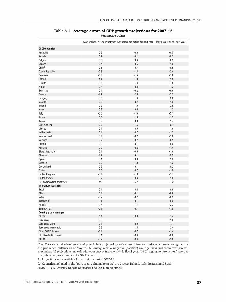
LESSONS FROM OECD FORECASTS DURING AND AFTER THE FINANCIAL CRISIS
OECD JOURNAL: ECONOMIC STUDIES – VOLUME 2014 © OECD 2015 37
Table A.1. Average errors of GDP growth projections for 2007-12Percentage points
May projection for current year November projection for next year May projection for next year
OECD countriesAustralia 0.2 -0.3 -0.5Austria 0.2 -0.1 -0.5Belgium 0.0 -0.4 -0.9Canada -0.4 -0.5 -1.2Chile1 0.5 0.7 0.5Czech Republic -0.3 -1.8 -2.4Denmark -0.8 -1.5 -1.8Estonia1 1.4 -1.0 1.8Finland -0.8 -1.4 -1.8France -0.4 -0.6 -1.2Germany 0.1 -0.2 -0.6Greece -1.2 -2.6 -3.7Hungary -0.6 -1.4 -3.0Iceland 0.3 0.7 -1.2Ireland -0.3 -1.9 -3.5Israel1 0.7 0.5 1.2Italy -0.5 -1.5 -2.1Japan 0.0 -1.3 -1.5Korea -0.2 -0.9 -1.4Luxembourg -0.8 -1.5 -2.4Mexico 0.1 -0.9 -1.6Netherlands 0.1 -0.7 -1.2New Zealand 0.4 -0.2 -1.0Norway -0.2 -0.7 -0.5Poland 0.2 0.1 0.0Portugal 0.2 -0.8 -1.4Slovak Republic 0.1 -0.8 -1.6Slovenia1 -1.2 -4.1 -2.3Spain 0.1 -0.9 -1.3Sweden 0.0 -1.0 -1.3Switzerland 0.3 0.1 -0.2Turkey 0.0 -0.7 -1.5United Kingdom -0.4 -1.0 -1.7United States -0.2 -0.4 -1.0OECD aggregate projection -0.1 -0.7 -1.2Non-OECD countriesBrazil -0.1 -0.4 -0.9China 0.1 -0.1 -0.6India -0.7 -0.7 -0.9Indonesia1 0.4 0.1 -0.2Russia -0.8 -1.7 -2.3South Africa1 -0.7 -0.7 -1.8Country group averages2
OECD -0.1 -0.9 -1.4Euro area -0.2 -1.1 -1.5Euro area: Core -0.1 -0.9 -1.1Euro area: Vulnerable -0.3 -1.5 -2.4Other OECD Europe -0.1 -0.7 -1.4OECD outside Europe 0.1 -0.4 -0.8BRIICS -0.2 -0.6 -1.0
Note: Errors are calculated as actual growth less projected growth at each forecast horizon, where actual growth isthe published outturn as at May the following year. A negative (positive) average error indicates over(under)-prediction. All projections are calendar year except India, which is fiscal year. “OECD aggregate projection” refers tothe published projection for the OECD area.
1. Projections only available for part of the period 2007-12.
2. Countries included in the “euro area: vulnerable group” are Greece, Ireland, Italy, Portugal and Spain.
Source: OECD, Economic Outlook Databases; and OECD calculations.
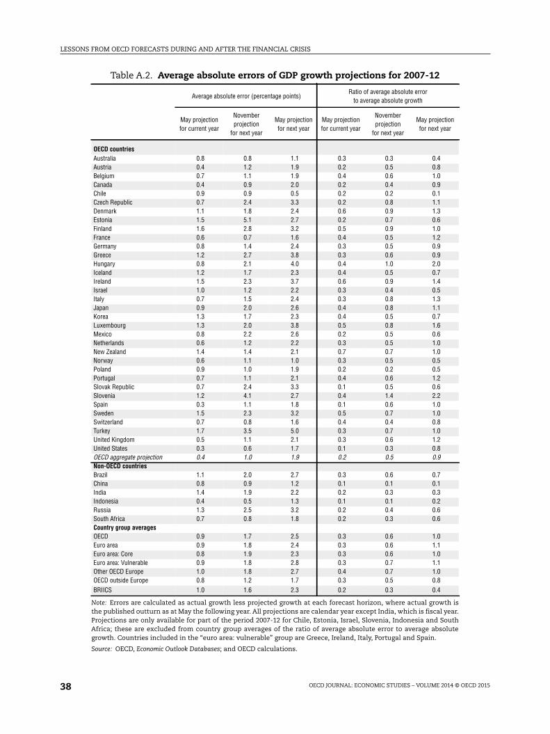
LESSONS FROM OECD FORECASTS DURING AND AFTER THE FINANCIAL CRISIS
OECD JOURNAL: ECONOMIC STUDIES – VOLUME 2014 © OECD 201538
Table A.2. Average absolute errors of GDP growth projections for 2007-12
Average absolute error (percentage points)Ratio of average absolute error
to average absolute growth
May projectionfor current year
Novemberprojection
for next year
May projectionfor next year
May projectionfor current year
Novemberprojection
for next year
May projectionfor next year
OECD countriesAustralia 0.8 0.8 1.1 0.3 0.3 0.4Austria 0.4 1.2 1.9 0.2 0.5 0.8Belgium 0.7 1.1 1.9 0.4 0.6 1.0Canada 0.4 0.9 2.0 0.2 0.4 0.9Chile 0.9 0.9 0.5 0.2 0.2 0.1Czech Republic 0.7 2.4 3.3 0.2 0.8 1.1Denmark 1.1 1.8 2.4 0.6 0.9 1.3Estonia 1.5 5.1 2.7 0.2 0.7 0.6Finland 1.6 2.8 3.2 0.5 0.9 1.0France 0.6 0.7 1.6 0.4 0.5 1.2Germany 0.8 1.4 2.4 0.3 0.5 0.9Greece 1.2 2.7 3.8 0.3 0.6 0.9Hungary 0.8 2.1 4.0 0.4 1.0 2.0Iceland 1.2 1.7 2.3 0.4 0.5 0.7Ireland 1.5 2.3 3.7 0.6 0.9 1.4Israel 1.0 1.2 2.2 0.3 0.4 0.5Italy 0.7 1.5 2.4 0.3 0.8 1.3Japan 0.9 2.0 2.6 0.4 0.8 1.1Korea 1.3 1.7 2.3 0.4 0.5 0.7Luxembourg 1.3 2.0 3.8 0.5 0.8 1.6Mexico 0.8 2.2 2.6 0.2 0.5 0.6Netherlands 0.6 1.2 2.2 0.3 0.5 1.0New Zealand 1.4 1.4 2.1 0.7 0.7 1.0Norway 0.6 1.1 1.0 0.3 0.5 0.5Poland 0.9 1.0 1.9 0.2 0.2 0.5Portugal 0.7 1.1 2.1 0.4 0.6 1.2Slovak Republic 0.7 2.4 3.3 0.1 0.5 0.6Slovenia 1.2 4.1 2.7 0.4 1.4 2.2Spain 0.3 1.1 1.8 0.1 0.6 1.0Sweden 1.5 2.3 3.2 0.5 0.7 1.0Switzerland 0.7 0.8 1.6 0.4 0.4 0.8Turkey 1.7 3.5 5.0 0.3 0.7 1.0United Kingdom 0.5 1.1 2.1 0.3 0.6 1.2United States 0.3 0.6 1.7 0.1 0.3 0.8OECD aggregate projection 0.4 1.0 1.9 0.2 0.5 0.9Non-OECD countriesBrazil 1.1 2.0 2.7 0.3 0.6 0.7China 0.8 0.9 1.2 0.1 0.1 0.1India 1.4 1.9 2.2 0.2 0.3 0.3Indonesia 0.4 0.5 1.3 0.1 0.1 0.2Russia 1.3 2.5 3.2 0.2 0.4 0.6South Africa 0.7 0.8 1.8 0.2 0.3 0.6Country group averagesOECD 0.9 1.7 2.5 0.3 0.6 1.0Euro area 0.9 1.8 2.4 0.3 0.6 1.1Euro area: Core 0.8 1.9 2.3 0.3 0.6 1.0Euro area: Vulnerable 0.9 1.8 2.8 0.3 0.7 1.1Other OECD Europe 1.0 1.8 2.7 0.4 0.7 1.0OECD outside Europe 0.8 1.2 1.7 0.3 0.5 0.8BRIICS 1.0 1.6 2.3 0.2 0.3 0.4
Note: Errors are calculated as actual growth less projected growth at each forecast horizon, where actual growth isthe published outturn as at May the following year. All projections are calendar year except India, which is fiscal year.Projections are only available for part of the period 2007-12 for Chile, Estonia, Israel, Slovenia, Indonesia and SouthAfrica; these are excluded from country group averages of the ratio of average absolute error to average absolutegrowth. Countries included in the “euro area: vulnerable” group are Greece, Ireland, Italy, Portugal and Spain.
Source: OECD, Economic Outlook Databases; and OECD calculations.
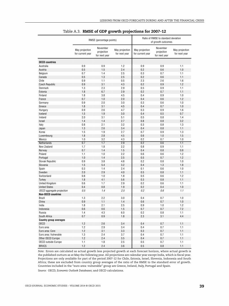
LESSONS FROM OECD FORECASTS DURING AND AFTER THE FINANCIAL CRISIS
OECD JOURNAL: ECONOMIC STUDIES – VOLUME 2014 © OECD 2015 39
Table A.3. RMSE of GDP growth projections for 2007-12
RMSE (percentage points)Ratio of RMSE to standard deviation
of growth outcomes
May projectionfor current year
Novemberprojection
for next year
May projectionfor next year
May projectionfor current year
Novemberprojection
for next year
May projectionfor next year
OECD countriesAustralia 0.9 0.9 1.2 0.9 0.9 1.1Austria 0.5 1.5 2.4 0.2 0.6 1.0Belgium 0.7 1.4 2.5 0.3 0.7 1.1Canada 0.5 1.3 2.5 0.2 0.6 1.1Chile 0.9 1.1 0.5 2.3 2.6 1.6Czech Republic 0.9 3.1 4.3 0.2 0.9 1.2Denmark 1.3 2.3 2.9 0.5 0.9 1.1Estonia 1.8 6.7 2.9 0.2 0.7 1.1Finland 1.8 3.8 4.5 0.4 0.9 1.0France 0.7 1.0 2.0 0.4 0.6 1.2Germany 0.9 2.0 3.0 0.3 0.6 1.0Greece 1.8 3.1 4.5 0.4 0.7 1.0Hungary 0.9 2.6 4.7 0.3 0.9 1.6Iceland 1.5 1.9 3.0 0.4 0.5 0.7Ireland 2.0 3.1 5.1 0.5 0.8 1.4Israel 1.4 1.4 2.7 0.8 0.8 3.2Italy 0.8 2.1 3.2 0.3 0.8 1.3Japan 1.3 2.6 3.4 0.4 0.8 1.1Korea 1.5 1.9 2.7 0.7 0.9 1.3Luxembourg 1.8 2.8 4.5 0.6 1.0 1.5Mexico 1.0 3.2 4.3 0.2 0.7 1.0Netherlands 0.7 1.7 2.9 0.2 0.6 1.1New Zealand 1.7 1.8 2.2 0.8 0.9 1.1Norway 0.7 1.4 1.5 0.4 0.8 0.8Poland 1.1 1.0 2.2 0.6 0.6 1.2Portugal 1.0 1.4 2.5 0.5 0.7 1.2Slovak Republic 0.9 3.8 4.8 0.2 0.8 1.0Slovenia 1.5 5.4 3.2 0.4 1.3 1.8Spain 0.3 1.4 2.4 0.1 0.6 1.0Sweden 2.0 2.9 4.0 0.5 0.8 1.1Switzerland 0.8 1.0 1.8 0.5 0.6 1.2Turkey 1.8 4.1 5.6 0.3 0.8 1.1United Kingdom 0.6 1.7 2.9 0.2 0.6 1.1United States 0.4 0.8 1.9 0.2 0.4 1.0OECD aggregate projection 0.5 1.4 2.5 0.2 0.6 1.1Non-OECD countriesBrazil 1.3 2.2 3.0 0.4 0.7 1.0China 0.9 1.1 1.4 0.6 0.7 1.0India 1.8 2.1 2.5 0.9 1.0 1.2Indonesia 0.6 0.6 1.5 0.7 0.7 7.2Russia 1.4 4.3 6.0 0.2 0.8 1.1South Africa 0.7 0.9 1.8 2.3 3.1 4.4Country group averagesOECD 1.2 2.6 3.4 0.4 0.7 1.1Euro area 1.2 2.9 3.4 0.4 0.7 1.1Euro area: Core 1.2 3.1 3.3 0.3 0.7 1.1Euro area: Vulnerable 1.3 2.4 3.7 0.4 0.7 1.1Other OECD Europe 1.2 2.4 3.5 0.4 0.7 1.1OECD outside Europe 1.1 1.8 2.5 0.5 0.7 1.1BRIICS 1.2 2.4 3.6 0.5 0.8 1.1
Note: Errors are calculated as actual growth less projected growth at each forecast horizon, where actual growth isthe published outturn as at May the following year. All projections are calendar year except India, which is fiscal year.Projections are only available for part of the period 2007-12 for Chile, Estonia, Israel, Slovenia, Indonesia and SouthAfrica; these are excluded from country group averages of the ratio of the RMSE to the standard error of growth.Countries included in the “euro area: vulnerable” group are Greece, Ireland, Italy, Portugal and Spain.
Source: OECD, Economic Outlook Databases; and OECD calculations.


![Andreas Schleicher [Oecd] 2011_building a High-quality Teaching Profession, Lessons From Around the World](https://static.fdocuments.us/doc/165x107/577d1cff1a28ab4e1e8b63c9/andreas-schleicher-oecd-2011building-a-high-quality-teaching-profession.jpg)
