ACTS 4302

FORMULA SUMMARY

Lessons 1-3: Introduction to Financial Derivatives, Forward and Futures Contracts.

1. If an asset pays no dividends, then the prepaid forward price is FP0,T = S0.2. If an asset pays dividends with amounts D1, . . . , Dn at times t1, . . . , tn, then the prepaid forward

price is

FP0,T = S0 −n∑i=1

Die−rti

3. If an asset pays dividends as a percentage of the stock price at a continuous (lease) rate δ, thenthe prepaid forward price is FP0,T = S0e

−δT .4. Cost of carry = r − δ5. F0,T = FP0,T e

rT

6. Implied fair price: the implied value of S0 when it is unknown based on an equation relating S0

to F0,T

7. Implied repo rate: implied value of r based on the price of a stock and a forward

8. Annualized forward premium = 1T ln

(F0,T

S0

)9. When dealing with Futures, we are always given an initial margin and a maintenance margin.

If the margin balance drops below the maintenance margin, a margin call is made requiring theinvestor deposit enough to bring the margin account balance to the initial margin.

10. Price to be paid at time T in a forward agreement made at time t to buy an item at time T :

Ft,T

11. Price of a forward on a non-dividend paying stock:

F0,T = S0erT

12. Price of a forward on a dividend paying stock with discrete dividends:

F0,T = S0erT − CumV alue(Div)

13. Price of a forward on a dividend paying stock with continuous dividends:

F0,T = S0e(r−δ)T

14. Price of a forward on a dividend paying stock with continuous dividends:

F0,T = S0e(r−δ)T

15. Price of a forward expressed in domestic currency to deliver foreign currency at x0 exchange rate:

F0,T = x0e(rd−rf )T

2

Lesson 4: Options

1. Assets(a) S0 = asset price at time 0; it is assumed the purchaser of the stock borrows S0 and must repay

the loan at the end of period T(b) Payoff(Purchased Asset)= ST(c) Profit(Purchased Asset)= ST − S0e

rT

(d) Payoff(Short Asset)= −ST(e) Profit(Short Asset)= −ST + S0e

rT

2. Calls(a) C0 = premium for call option at time 0; it is assumed the purchaser of the call borrows C0

and must repay the loan when the option expires(b) Payoff(Purchased Call)= max 0, ST −K(c) Profit(Purchased Call)= max 0, ST −K − C0e

rT

(d) Payoff(Written Call)= −max 0, ST −K(e) Profit(Written Call)= −max 0, ST −K+ C0e

rT

3. Puts(a) P0 = premium for put option at time 0; it is assumed the purchaser of the put borrows P0

and must repay the loan when the option expires(b) Payoff(Purchased Put)= max 0,K − ST (c) Profit(Purchased Put)= max 0,K − ST − P0e

rT

(d) Payoff(Written Put)= −max 0,K − ST (e) Profit(Written Put)= −max 0,K − ST + P0e

rT

3

Lesson 5: Option Strategies

1. Floor: buying an asset with a purchased put option2. Cap: short selling an asset with a purchased call option3. Covered put (short floor): short selling an asset with a written put option4. Covered call (short cap): buying an asset with a written call option5. Synthetic Forward: combination of puts and calls that acts like a forward; purchasing a call

with strike price K and expiration date T and selling a put with K and T guarantees a purchaseof the asset for a price of K at time T

6. Short synthetic forward: purchasing a put option with strike price K and expiration date Tand writing a call option with strike price K and expiration date T

7. No Arbitrage Principle: If two different investments generate the same payoff, they must havethe same cost.

8. C(K,T ) = price of a call with an expiration date T and strike price K9. P (K,T ) = price of a put with an expiration date T and strike price K

10. Put-Call parity: C0 − P0 = C(K,T )− P (K,T ) = (F0,T −K)vT

11. If the asset pays no dividends, then the no-arbitrage forward price is F0,T = S0erT ⇒ S0 = F0,T v

T .

12. C(K,T ) +KvT = PK, T ) + S0

13. Spread: position consisting of only calls or only puts, in which some options are purchased andsome written

14. Bull: investor betting on increase in market value of an asset15. Bull spread: purchased call with lower strike price K1 and written call with higher strike price

K2

16. A bull spread can also be created by a purchased put with strike price K1 and a written put withstrike price K2.

17. Bear: an investor betting on a decrease in market value of an asset18. Bear spread: written call with lower strike price K1 and purchased call with higher strike price

K2

19. Ratio spread: purchasing m calls at one strike price K1 and writing n calls at another strikeprice K2

20. Box spread: using options to create a synthetic long forward at one price and a synthetic shortforward at a different price

21. Purchased collar: purchased put option with lower strike price K1 and written call option withhigher strike price K2

22. Collar width: difference between the call and put strikes23. Written collar: writing a put option with lower strike price K1 and purchasing a call option with

higher strike price K2

24. Zero-cost collar: choosing the strike prices so that the cost is 025. Purchased straddle: purchased call and put with the same strike price K26. Written straddle: written call and put with the same strike price K27. Purchased strangle: purchased put with lower strike price K1 and purchased call with a higher

strike price K2

28. Written strangle: written put with lower strike price K1 and written call with a higher strikeprice K2

29. Butterfly spread: a written straddle with a purchased strangle30. Asymmetric butterfly spread: purchasing λ calls with strike price K1, purchasing 1− λ calls

with strike price K3, and writing 1 call with strike price K2 where λ =K3 −K2

K3 −K1and K1 < K2 < K3

4

Lesson 6: Put-Call Parity

1. Call option payoff:max(0, ST −K)

2. Put option payoff:max(0,K − ST )

3. General Put Call Parity (PCP):

C(S,K, T )− P (S,K, T ) = (F0,T −K)e−rT

4. PCP for a non-dividend paying stock:

C(S,K, T )− P (S,K, T ) = S0 −Ke−rT

5. PCP for a dividend paying stock with discrete dividends:

C(S,K, T )− P (S,K, T ) = S0 − PV0,T (Div)−Ke−rT

6. PCP for a dividend paying stock with continuous dividends:

C(S,K, T )− P (S,K, T ) = S0e−δT −Ke−rT

7. Pre-paid forward at time t:FPt,T (S) = e−r(T−t)Ft,T

8. Call option written at time t which lets the purchaser elect to receive ST in return for QT at timeT :

C(St, Qt, T − t)9. Put option written at time t which lets the purchaser elect to give ST in return for QT at time T :

P (St, Qt, T − t)10. PCP for exchange options:

C(St, Qt, T − t)− P (St, Qt, T − t) = FPt,T (S)− FPt,T (Q)

P (St, Qt, T − t) = C(Qt, St, T − t)C(St, Qt, T − t)− C(Qt, St, T − t) = FPt,T (S)− FPt,T (Q)

11. Call-Put relationship in ”domestic” currency:

KPd

(1

x0,

1

K,T

)= Cd(x0,K, T )

KCd

(1

x0,

1

K,T

)= Pd(x0,K, T )

12. Call-Put relationship in ”foreign” and ”domestic” currency:

Kx0Pf

(1

x0,

1

K,T

)= Cd(x0,K, T )

Kx0Cf

(1

x0,

1

K,T

)= Pd(x0,K, T )

13. PCP for currency options with x0 as a spot exchange rate:

Cd(x0,K, T )− Pd(x0,K, T ) = x0e−rfT −Ke−rdT

Cf

(1

x0,

1

K,T

)− Pf

(1

x0,

1

K,T

)=

1

x0e−rdT − 1

Ke−rfT

5

Lesson 7: Comparing Options

1. Inequalities for American and European call options:

S ≥ CAmer(S,K, T ) ≥ CEur(S,K, T ) ≥ max(0, FP0,T (S)−Ke−rT )

2. Inequalities for American and European put options:

K ≥ PAmer(S,K, T ) ≥ PEur(S,K, T ) ≥ max(0,Ke−rT − FP0,T (S))

3. Direction property: If K1 ≤ K2 then

C(K1) ≥ C(K2) and P (K1) ≤ P (K2)

4. Slope property: If K1 ≤ K2 then

C(K1)− C(K2) ≤ (K2 −K1) and P (K2)− P (K1) ≤ (K2 −K1)

5. Convexity property: If K1 ≤ K2 ≤ K3 then

C(K2)− C(K3)

K3 −K2≤ C(K1)− C(K2)

K2 −K1⇔ C(K2) ≤ C(K1)(K3 −K2) + C(K3)(K2 −K1)

K3 −K1

P (K2)− P (K1)

K2 −K1≤ P (K3)− P (K2)

K3 −K2⇔ P (K2) ≤ P (K1)(K3 −K2) + P (K3)(K2 −K1)

K3 −K1

6. Maximum possible value of the difference between the two calls:

max(C(K1)− C(K2)) = e−rT (K2 −K1)

6

Lesson 8: Binomial Trees - Stock, One Period

The formulas below are true for calls and puts. We use calls in the notation.

1. Pricing an option using risk-neutral probability p∗ of an increase in stock price

C = e−rh (p∗Cu + (1− p∗)Cd) , where

p∗ =e(r−δ)h − du− d

1− p∗ =u− e(r−δ)h

u− d2. Replicating portfolio for the option:

C = S∆ +B, where

∆ =

(Cu − CdS(u− d)

)e−δh

B = e−rh(uCd − dCuu− d

)3. To avoid arbitrage, u and d must satisfy:

d < e(r−δ)h < u

4. If σ is the annualized standard deviation of stock price movements, then

u = e(r−δ)h+σ√h

d = e(r−δ)h−σ√h

p∗ =1

1 + eσ√h

1− p∗ =1

1 + e−σ√h

5. If a call (put) does not pay off at the upper(lower) node, ∆ = 0. If a call or a put pays off at boththe upper and the lower node, ∆ = 1.

6. If the option always pays off, one could use the Put Call Parity to evaluate its premium (theopposite option will be zero).

7

Lesson 9: Binomial Trees - General

1. For options on futures contracts:

u = eσ√h, d = e−σ

√h

p∗ =1− du− d

∆ =Cu − CdF (u− d)

, B = C

C = e−rh (p∗Cu + (1− p∗)Cd)

8

Lesson 10: Risk-Neutral Pricing (Other valuation methods of pricing options).

1. The following notation is used when pricing with true probabilities:γ - rate of return for the optionα - rate of return for the stockp - (true) probability that the stock will increase in value

2. Probability that the stock will increase in value

p =e(α−δ)h − du− d

3. Accumulated option value equals accumulated replicating portfolio value:

(S∆ +B)eγh = S∆eαh +Berh ⇔ Ceγh = S∆eαh +Berh

4. Often used to find the annual return of an option γ (using call notation):

C = e−γh (pCu + (1− p)Cd) = e−rh (p∗Cu + (1− p∗)Cd)

For example, if Cd = 0, e−γhp = e−rhp∗

5. In the tree based on forward prices, δ does not affect p∗ or p.

6. The following notation is used when pricing with utility:

7. If SH and SL are the stock prices in the high and low state, and QH , QL - the prices of securitiespaying $1 when the state H or L occurs, then the state prices are calculated as follows:

QH =S0e−δh − e−rhSLSH − SL

and QL =e−rhSH − S0e

−δh

SH − SL8. If CH , CL - are high and low values of a derivative C, based on the stock prices, then C =CHQH + CLQL.

9. If p is the true probability of state H and UH , UL are the utility values, expressed in terms ofdollars today, that an investor attach to $1 received in the up and down state after 1 period, then

QH = pUH , QL = (1− p)UL

10. Initial value of stock using utility:

C0 = pUHCH + (1− p)ULCL = QHCH +QLCL

11. Effective annual return of a risk free investment using utility, assuming a one-year horizon:

r =1

QH +QL− 1

12. Effective annual return of a stock using utility, assuming a one-year horizon:

α =pCH + (1− p)CL

pUHCH + (1− p)ULCL− 1 =

pCH + (1− p)CLQHCH +QLCL

− 1

9

13. Risk-neutral probabilities in terms of true probabilities and utility:

p∗ =pUH

pUH + (1− p)UL=

QHQH +QL

p∗ = QH(1 + r) = pUH(1 + r)

14. True probabilities in terms of risk-neutral probabilities and utility:

p =p∗UL

p∗UL + (1− p∗)UH

10

Lesson 11: Binomial Trees: Miscellaneous Topics

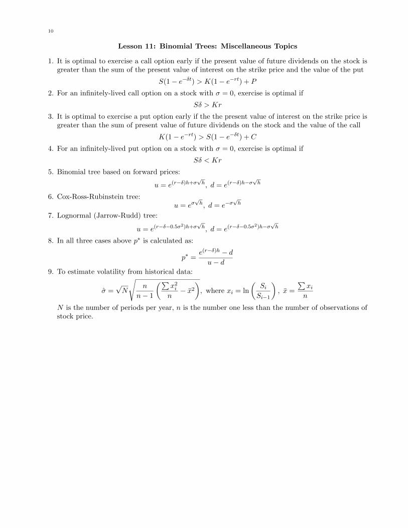
1. It is optimal to exercise a call option early if the present value of future dividends on the stock isgreater than the sum of the present value of interest on the strike price and the value of the put

S(1− e−δt) > K(1− e−rt) + P

2. For an infinitely-lived call option on a stock with σ = 0, exercise is optimal if

Sδ > Kr

3. It is optimal to exercise a put option early if the the present value of interest on the strike price isgreater than the sum of present value of future dividends on the stock and the value of the call

K(1− e−rt) > S(1− e−δt) + C

4. For an infinitely-lived put option on a stock with σ = 0, exercise is optimal if

Sδ < Kr

5. Binomial tree based on forward prices:

u = e(r−δ)h+σ√h, d = e(r−δ)h−σ

√h

6. Cox-Ross-Rubinstein tree:u = eσ

√h, d = e−σ

√h

7. Lognormal (Jarrow-Rudd) tree:

u = e(r−δ−0.5σ2)h+σ√h, d = e(r−δ−0.5σ2)h−σ

√h

8. In all three cases above p∗ is calculated as:

p∗ =e(r−δ)h − du− d

9. To estimate volatility from historical data:

σ =√N

√n

n− 1

(∑x2i

n− x2

), where xi = ln

(SiSi−1

), x =

∑xin

N is the number of periods per year, n is the number one less than the number of observations ofstock price.

11

Lesson 12: Modeling stock prices with the lognormal distribution

For a stock whose price St follows a lognormal model:

1. Assume that

ln(St/S0) ∈ N (m, v2), where m = (α− δ − 0.5σ2)t, v2 = σ2t

2. The expected value is

E[St|S0] = S0e(µ+0.5σ2)t = S0e

(α−δ)t

3. The median price of the stock t years

S(0.5) = S0eµt = S0e

(α−δ−0.5σ2)t

4. If Z ∈ N(m, v2), then the 100(1− α)% confidence interval is defined to be(m− zα/2v,m+ zα/2v

), where zα/2 is the number such that

P[Z > zα/2

]=α

2

5. Since St/S0 = eZ(t), Z ∈ N(m, v2), the confidence interval for St will be(S0e

m−z1−α/2v, S0em+z1−α/2v

)6. Probabilities of payoffs and partial expectations of stock prices are:

Pr(St < K) = N(−d2)

Pr(St > K) = N(d2)

PE[St|St < K] = S0e(α−δ)tN(−d1)

E[St|St < K] =S0e

(α−δ)tN(−d1)

N(−d2)

PE[St|St > K] = S0e(α−δ)tN(d1)

E[St|St > K] =S0e

(α−δ)tN(d1)

N(d2)

E[St|K1 < St < K2] =S0e

(α−δ)tN(d1

(1))− S0e

(α−δ)tN(d1

(2))

N(d2

(1))−N

(d2

(2))

7. d1 and d2 are defined by

d1 =ln(S0K

)+ (α− δ + 0.5σ2)t

σ√t

d2 =ln(S0K

)+ (α− δ − 0.5σ2)t

σ√t

d2 = d1 − σ√t

8. Expected call option payoff:

E[max(0, St −K)] = S0e(α−δ)tN(d1)−KN(d2)

9. Expected put option payoff:

E[max(0,K − St)] = KN(−d2)− S0e(α−δ)tN(−d1)

12

Lesson 13: Fitting stock prices to a lognormal distribution

1. If xi are observed stock prices adjusted to remove the effect of dividends, the estimate for thecontinuously compounded annual return is:

α = µ+ 0.5σ2, where

µ = Nx

σ =√N

√n

n− 1

(∑x2i

n− x2

)N is the number of periods per year, n is the number one less than the number of observations of

stock price, xi = ln(

SiSi−1

).

2. A normal probability plot graphs each observation against its percentile of the normal distribu-tion on the vertical axis. However, the vertical axis is scaled according to the standard normaldistribution rather than linearly.

13

Lesson 14: The Black-Scholes Formula

1. Assumptions of the Black-Scholes formula:• Continuously compounded returns on the stock are normally distributed and independent over

time.• Continuously compounded returns on the strike asset (e.g., the risk-free rate) are known and

constant.• Volatility is known and constant.• Dividends are known and constant.• There are no transaction costs or taxes• It is possible to short-sell any amount of stock and to borrow any amount of money at the

risk-free rate.2. General form of the Black-Scholes Formula

C(S,K, σ, r, t, δ) = FP (S)N(d1)− FP (K)N(d2), where

d1 =ln(FP (S)/FP (K)

)+ 1

2σ2t

σ√t

, d2 = d1 − σ√t

Here σ is the volatility of the pre-paid forward price on the stock. Note that it is equal to thevolatility of the stock in case of the continuous dividends, but otherwise differs from it.

3. The Black-Scholes Formula for a stock

C = Se−δtN(d1)−Ke−rtN(d2)

P = Ke−rtN(−d2)− Se−δtN(−d1), where

d1 =ln (S/K) + (r − δ + 1

2σ2)t

σ√t

, d2 = d1 − σ√t

4. The Black-Scholes Formula for a currency asset

C = xe−rf tN(d1)−Ke−rdtN(d2)

P = Ke−rdtN(−d2)− xe−rf tN(−d1), where

d1 =ln (x/K) + (rd − rf + 1

2σ2)t

σ√t

, d2 = d1 − σ√t

5. The Black-Scholes Formula for futures

C = Fe−rtN(d1)−Ke−rtN(d2)

P = Ke−rtN(−d2)− Fe−rtN(−d1), where

d1 =ln (F/K) + 1

2σ2t

σ√t

, d2 = d1 − σ√t

14

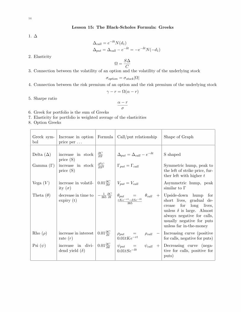
Lesson 15: The Black-Scholes Formula: Greeks

1. ∆

∆call = e−δtN(d1)

∆put = ∆call − e−δt = −e−δtN(−d1)

2. Elasticity

Ω =S∆

C3. Connection between the volatility of an option and the volatility of the underlying stock

σoption = σstock|Ω|4. Connection between the risk premium of an option and the risk premium of the underlying stock

γ − r = Ω(α− r)5. Sharpe ratio

α− rσ

6. Greek for portfolio is the sum of Greeks7. Elasticity for portfolio is weighted average of the elasticities8. Option Greeks

Greek sym-bol

Increase in optionprice per . . .

Formula Call/put relationship Shape of Graph

Delta (∆) increase in stockprice (S)

∂C∂S ∆put = ∆call − e−δt S shaped

Gamma (Γ) increase in stockprice (S)

∂2C∂S2 Γput = Γcall Symmetric hump, peak to

the left of strike price, fur-ther left with higher t

Vega (V ) increase in volatil-ity (σ)

0.01∂C∂σ Vput = Vcall Asymmetric hump, peaksimilar to Γ

Theta (θ) decrease in time toexpiry (t)

− 1365

∂C∂t θput = θcall +

rKe−rt−δSe−δt365

Upside-down hump forshort lives, gradual de-crease for long lives,unless δ is large. Almostalways negative for calls,usually negative for putsunless far in-the-money

Rho (ρ) increase in interestrate (r)

0.01∂C∂r ρput = ρcall −0.01tKe−rt

Increasing curve (positivefor calls, negative for puts)

Psi (ψ) increase in divi-dend yield (δ)

0.01∂C∂δ ψput = ψcall +

0.01tSe−δtDecreasing curve (nega-tive for calls, positive forputs)

15

Lesson 16: The Black-Scholes formula: applications and volatility

1. Let Ct be the price of a call option at time t. Then the profit on a call sold at time 0 < t < T is:

Profit = Ct − C0ert

2. A bull spread is the purchase of a call (or put) together with the sale of an otherwise identicalhigher-strike call (or put).

3. A calendar spread consists of selling a call and buying another call with the same strike price onthe same stock but a later expiry date.

4. Implied volatility is the opposite of historical volatility, which is estimated based on the stock data.The implied volatility is calculated (actually, back out) based on option prices and a pricing model.

16

Lesson 17: Delta-Hedging

1. Overnight profit on a delta-hedged portfolio has three components:1. The change in the value of the option.2. ∆ times the change in the price of the stock.3. Interest on the borrowed money.

Profit = −(C(S1)− C(S0)) + ∆(S1 − S0)−(er/365 − 1

)(∆S0 − C(S0))

2. Price movement with no gain or loss to delta-hedger: the money-maker would break even if thestock moves by about one standard deviation around the mean to either

S + Sσ√h or S − Sσ

√h

3. Delta-gamma-theta approximation

C(St+h) = C(St) + ∆ε+1

2Γε2 + hθ

4. Black-Scholes equation for market maker profit (an approximation of the profit formula above):

Profit = −(1

2Γε2︸ ︷︷ ︸

changein stock

priceeffect

+ hθ︸︷︷︸timedecay

ofoption

+ rh(∆S − C(S))︸ ︷︷ ︸interest effect

)

5. Boyle-Emanuel periodic variance of return when rehedging every h in period i:

V ar (Rh,i) =1

2

(S2σ2Γh

)26. Boyle-Emanuel annual variance of return when rehedging every h in period i:

V ar (Rh,i) =1

2

(S2σ2Γ

)2h

7. Formulas for Greeks of binomial trees

∆(S, 0) =

(Cu − CdS(u− d)

)e−δh

Γ(S, 0) ≈ Γ(S, h) =∆(Su, h)−∆(Sd, h)

S(u− d)

θ(S, 0) =C(Sud)− C(S, 0)−∆(S, 0)ε− 0.5Γ(S, 0)ε2

2h

17

Lesson 18: Asian, Barrier, and Compound Options.

1. Geometric averages of stock pricesThe n stock prices S(1), S(2), · · · , S(n) are not independent, but in the Black-Scholes framework

there is no memory, so the variables Q(t) = S(t)/S(t− 1) are independent.

If G =

(n∏k=1

S(k)

)1/n

and U = lnG

Then

E[U ] = ln(S(0)) + m, V ar(U) = v2

E[G(S)] = S(0)em+ 12v2

V ar (G(S)) = E[G(S)]2(ev

2 − 1)

= S(0)2e2m+v2(ev

2 − 1), where

m =n+ 1

2m, v2 =

(n+ 1)(2n+ 1)

6nv2

m = (α− δ − 0.5σ2)t, v2 = σ2t

2. Parity relationship for barrier options:

Knock-in option + Knock-out option = Ordinary option

3. Maxima and MinimaThe following properties will be useful in expressing various claims payoffs:

(a) max(S,K) = S + max(0,K − S) = K +max(0, S −K)(b) max(cS, cK) = cmax(S,K), c > 0(c) min(S,K) + max(S,K) = S +K ⇒ min(S,K) = S +K −max(S,K)

4. Parity relationships for compound options:

CallOnCall(S,K, x, σ, r, t1, T, δ)− PutOnCall(S,K, x, σ, r, t1, T, δ) = C(S,K, σ, r, T, δ)− xe−rt1

CallOnPut(S,K, x, σ, r, t1, T, δ)− PutOnPut(S,K, x, σ, r, t1, T, δ) = P (S,K, σ, r, T, δ)− xe−rt1

5. Value of American call option with one discrete dividend:

S0 −Ke−rt1 + CallOnPut(S,K,D −K

(1− e−r(T−t1)

))

18

Lesson 19: Gap, Exchange and Other Options.

1. Black-Scholes formula for all-or-nothing options:

Option Name Value Delta

S|S > K asset-or-nothing call Se−δTN(d1) e−δTN(d1) + e−δT e−d1

2/2

σ√

2πT

S|S < K asset-or-nothing put Se−δTN(−d1) e−δTN(−d1)− e−δT e−d12/2

σ√

2πT

c|S > K cash-or-nothing call ce−rTN(d2) ce−rT e−d22/2

Sσ√

2πT

c|S < K cash-or-nothing put ce−rTN(−d2) −ce−rT e−d22/2

Sσ√

2πT

2. Black-Scholes formula for gap options:Use K1 (the strike price) in the formula for C and P .Use K2 in formula for d1

C = Se−δtN(d1(K2))−K1e−rtN(d2(K2))

P = K1e−rtN(−d2(K2))− Se−δtN(−d1(K2)), where

d1 =ln (S/K2) + (r − δ + 1

2σ2)t

σ√t

, d2 = d1 − σ√t

∆ = e−δTN(d1) + (K2 −K1)e−rTe−d2

2/2

Sσ√

2πT

3. Exchange options: Recieve option S for option Q.

Volatility: σ2 = σ2S + σ2

Q − 2ρσSσQ

C(S,Q, T ) = Se−δSTN(d1)−Qe−δQTN(d2), where

d1 =ln(FP (S)/FP (Q)

)+ 0.5σ2T

σ√T

=ln (S/Q) + (δQ − δS + 0.5σ2)T

σ√T

d2 = d1 − σ√T

4. Chooser options:

V = C(S,K, T ) + e−δ(T−t)P(S,Ke−(r−δ)(T−t), t

)= P (S,K, T ) + e−δ(T−t)C

(S,Ke−(r−δ)(T−t), t

)5. Forward start options:

If you can purchase a call option with strike price cSt at time t expiring at time T , then thevalue of the forward start option is

V = Se−δTN(d1)− cSe−r(T−t)−δtN(d2)

where d1 and d2 are computed using T − t as time to expiry.

19

Lesson 20: Monte Carlo Valuation

Generating a log-normal random numberA standard normal random variable may be generated as

12∑i=1

ui − 6, or as N−1(ui)

General steps for simulating the stock value at time t with initial price S0:

(1) Given u1, u2, · · · , un uniformly distributed on [0, 1],(2) Find z1, z2, · · · , zn where zj = N−1(ui) normally distributed with m = 0, v = 1(3) Generate n1, n2, · · · , nn where nj = m+ vzj , m = (α− δ − 0.5σ2)t, v2 = σ2t

(4) Then S(j)t = S0e

nj and St = 1n

∑nj=1 S

(j)t

A Lognormal Model of Stock PricesAn expression for the stock price:

St = S0 exp(α− δ − 0.5σ2

)t+ σ

√tz, z ∈ N(0, 1)

The expected stock price:

E[St] = S0 exp

(α− δ − 0.5σ2

)t+

1

2σ2t

= S0 exp (α− δ) t

The median stock price:S0 exp

(α− δ − 0.5σ2

)t

Variance Reduction MethodsFor the control variate method,

X∗ = X +(E[Y ]− Y

)V ar(X∗) = V ar(X) + V ar(Y )− 2Cov(X, Y )

For the Boyle modification,

X∗ = X + β(E[Y ]− Y

),

V ar(X∗) = V ar(X) + β2V ar(Y )− 2βCov(X, Y )

β is chosen to minimize the expression for V ar(X∗):

β =Cov(X, Y )

V ar(Y )=

∑xiyi − XY /n∑y2i − Y 2/n

20

Lesson 21: Brownian Motion.

Part 1. Brownian Motion.

Assume that

1. The continuously compounded rate of return for a stock is α2. The continuously compounded dividend yield is δ3. The volatility is σ

Brownian motion: Z(t) - a collection of random variable, defined by the following properties:

1. Z(0) = 02. Let t be the latest time for which you know Z(t). Then Z(t + s)|Z(t) has a normal distribution

with m = Z(t) and v2 = s3. Increments are independent: Z(t+ s1)− Z(t) is independent of Z(t)− Z(t− s2)4. More generally, non-overlapping increments are independently distributed, i.e. for t1 < t2 ≤ t3 <t4, Z(t2)− Z(t1) and Z(t4)− Z(t3) are independent.

5. Z(t) is continuous in t.

Arithmetic Brownian motion: Let Z(t) be Brownian motion. Then

X(t) = X(0) + αt+ σZ(t) or dX(t) = αdt+ σdZ(t)

is Arithmetic Brownian motion. Here α is the drift and σ is the volatility of the process.Let t be the latest time for which you know X(t). Then

1. X(t+ s)|X(t) has a normal distribution with m = X(t) + αs and v2 = σ2s2. X(t+ s)−X(t) has a normal distribution with m = αs and v2 = σ2s3. Non-overlapping increments are independently distributed, i.e. for t1 < t2 < t3 < t4, X(t2)−X(t1)

and X(t4)−X(t3) are independent.4. If X(0) = 0, then for any t, u such that 0 < t < u, Cov(X(t), X(u)) = σ2t

Geometric Brownian motion:

X(t) follows Geometric Brownian motion if lnX(t) follows Arithmetic Brownian motion.Let t be the latest time for which you knowX(t). Then lnX(t+s)/X(t)|X(t) has a normal distributionwith m = (α− δ − 0.5σ2)s and v2 = σ2sLet S(t) be the time t price of the stock. Then

1. The continuously compounded expected increase in the stock price is α− δ. This means

E[S(t)] = S(0)e(α−δ)t

2. The increase in the stock price is also known as the capital gains return.3. The total return on the stock is the sum of the capital gains return and the dividend yield4. The geometric Brownian motion followed by the stock price is

dS(t)

S(t)= (α− δ)dt+ σdZ(t)

GBM is an example of an Ito process.5. The associated arithmetic Brownian motion followed by lnS(t) is

d (lnS(t)) =(α− δ − 0.5σ2

)dt+ σdZ(t)

6. When evaluating probabilities for ranges of S(t), look up the normal table using the followingparameters:

m =(α− δ − 0.5σ2

)t, v2 = σ2t

21

All of the following are equivalent:

X(t) follows a geometric Brownian motion with drift ξ and volatility σ

dX(t)

X(t)= ξdt+ σdZ(t)

d (lnX(t)) = (ξ − 0.5σ2)dt+ σdZ(t)

lnX(t)|X(0) is N(lnX(0) + (ξ − 0.5σ2)t, σ2t

)lnX(t)− lnX(0) = (ξ − 0.5σ2)t+ σZ(t)

lnX(t)− lnX(0) =

∫ t

0(ξ − 0.5σ2)ds+

∫ t

0σdZ(s)

X(t) = X(0)e(ξ−0.5σ2)t+σZ(t)

X(t)−X(0) =

∫ t

0ξX(s)ds+

∫ t

0σX(s)dZ(s)

Stock price modeling: Let S(t) be the time t price of a stock. Assume:

1. The continuously compounded expected rate of return is α.2. The continuously compounded dividend yield is δ.3. The volatility is σ, in other words V ar (lnS(t)|S(0)) = σ2t.

Then ξ = α = δ is the continuously compounded rate of increase in the stock price. All the statementsabove for geometric Brownian motion with drift ξ and volatility σ hold. For example,

X(t) follows a geometric Brownian motion with drift ξ and volatility σ

dS(t)

S(t)= (α− δ)dt+ σdZ(t)

d (lnS(t)) = (α− δ − 0.5σ2)dt+ σdZ(t)

Multiplication rules:

dt× dt = dt× dZ = 0

dZ × dZ = dt

dZ × dZ ′ = ρdt

22

Lesson 22: Ito’s Lemma. Black-Scholes Equation.

Any process of the form

dS(t) = ξ (S(t), t) dt+ σ (S(t), t) dZ(t)

is called an Ito process.

Ito’s Lemma

dC(S, t) = CSdS + 0.5CSS(dS)2 + Ctdt

Black-Scholes Equation

1

2σ2S2CSS + (r − δ)SCS + Ct = rC

Using greeks, the Black-Scholes Equation is:

∆S(r − δ) + 0.5ΓS2σ2 + θ = rC

Sharpe ratioSharpe ratio: Express process in the following form:

dX

X= (α (t,X(t))− δ (t,X(t))) dt+ σ (t,X(t)) dZ(t)

Then the Sharpe ratio is

φ (t,X(t)) =α (t,X(t))− rσ (t,X(t))

• The Sharpe ratio is based on the total return. Do not subtract the dividend rate from α (t,X(t))in the numerator of the Sharpe ratio.• For geometric Brownian motion, the Sharpe ratio is the constant

η =α− rσ

• The Sharpe ratio is the same for all processes based on the same Z(t).

Risk-neutral Processes.The true Ito process

dS(t) = (α(t, S(t))− δ(t, S(t))) dt+ σ(t, S(t))dZ(t)

can be translated into the risk-neutral process of the form:

dS(t) = (r(t)−δ(t, S(t)))dt+σ(t, S(t))dZ(t), dZ(t) = dZ(t)+ηdt, η =α(t, S(t))− r(t)

σ(t, S(t))− Sharpe ratio

Z(t) follows an arithmetic Brownian motion.

Formulas for Sa.Expected value

E [S(T )a] = S(0)ae[a(α−δ)+0.5a(a−1)σ2]T

Forward price and pre-paid forward price

F0,T (Sa) = S(0)ae[a(r−δ)+0.5a(a−1)σ2]T

FP0,T (Sa) = e−rTS(0)ae[a(r−δ)+0.5a(a−1)σ2]T

Ito processd(Sa)

Sa=(a(α− δ) + 0.5a(a− 1)σ2

)dt+ aσdZ(t)

Total return rate

γ = a(α− δ) + r

23

Ornstein-Uhlenbeck process: Definition

dX(t) = λ (α−X(t)) dt+ σdZ(t)

Integral

X(t) = X(0)e−λt + α(

1− e−λt)

+ σ

∫ t

0eλ(s−t)dZ(s)

24

Lesson 23: Binomial tree models for interest rates.

Let Pt(T, T+s) be the price, to be paid at time T , for an agreement at time t to purchase a zero-couponbond for 1 issued at time T maturing at time T + s, t < T . Omit subscript if t = T.Let Ft,T (P (T, T + s)) be the forward price at time t for an agreement to buy a bond at time Tmaturing at time T + s. Then

Ft,T (P (T, T + s)) =P (t, T + s)

P (t, T )

This section considers:

(1) Interest rate binomial trees(2) The Black-Derman-Toy model for interest rates(3) Pricing forwards and caps (via caplets)

25

Lesson 24: The Black formula for bond options.

Black formulaLet C (F, P (0, T ), σ, T ) be a call on a bond at time 0 that allows to buy a bond at time T whichmatures at time T + s.Let P (F, P (0, T ), σ, T ) be a put on a bond at time 0 that allows to sell a bond at time T whichmatures at time T + s.F = F0,T (P (T, T + s))

C (F, P (0, T ), σ, T ) = P (0, T ) (FN(d1)−KN(d2))

P (F, P (0, T ), σ, T ) = P (0, T ) (KN(−d2)− FN(−d1)) ,

where

d1 =ln(F/K) + 0.5σ2T

σ√T

d2 = d1 − σ√T

and σ is the volatility of the T -year forward price of the bond.

Black formula for caplets:

(1) Caplet - protects a floating rate borrower by paying the amount by which the prevailing rateis greater than the cap

(2) Each caplet is 1 +KR puts with strike 11+KR

.

Black formula for floorlets:

(1) Floorlet - protects a floating rate lender by paying the amount by which the prevailing rate isless than the floor

(2) Each floorlet is 1 +KR calls with strike 11+KR

.

26

Lesson 20: Equilibrium interest rate models: Vasicek and Cox-Ingersoll-Ross.

Let P (r, t, T ) be the price of a zero-coupon bond purchased at time t and maturing at time T whenthe short term rate is r.Hedging formulas:

Duration hedging bond 1 with bond 2: N = −(T1 − t)P (t, T1)

(T2 − t)P (t, T2)

Delta hedging bond 1 with bond 2: N = −Pr(r, t, T1)

Pr(r, t, T2)

N = −B(t, T1)P (r, t, T1)

B(t, T2)P (r, t, T2)for Vasicek and Cox-Ingersoll-Ross

Yield to maturity on a zero-coupon bond:

R(t, T ) =ln (1/P (r, t, T ))

T − t=

ln (P (r, t, T ))

t− T, r(t) = lim

T→tR(t, T )

Differential equation for bond prices:If the interest rate process is dr = a(r)dt+ σ(r)dZ(t), then

dP

P= α(r, t, T )dt− q(r, t, T )dZ(t)

where

α(r, t, T ) =a(r)Pr + 0.5σ(r)2Prr + Pt

P

= −a(b− r)B(t, T ) + 0.5σ(r)2B(t, T )2 +PtP

for Vasicek and Cox-Ingersoll-Ross

q(r, t, T ) = −Prσ(r)

P= B(t, T )σ(r) for Vasicek and Cox-Ingersoll-Ross

Risk-neutral process:dr = (a(r) + φ(r, t)σ(r)) dt+ σ(r)dZ, dZ(t) = dZ(t)− φ(r, t)dt, φ(r, t) is the Sharpe ratio.

Black-Scholes Equation analog for bond prices:

1

2σ(r)2Prr + (a(r) + φ(r, t)σ(r))Pr + Pt − rP = 0

Sharpe ratio:

General φ(r, t) =α(r, t, T )− rq(r, t, T )

Vasicek φ(r, t) = φ it is constant

Cox-Ingersoll-Ross φ(r, t) = φ√r/σ (φ and σ are constant, σ =

σ(r)√r

)

Definitions of interest rate models:

General dr = a(r)dt+ σ(r)dZ(t)

Rendleman-Bartter dr = ardt+ σrdZ(t)

Vasicek dr = a(b− r)dt+ σdZ(t)

Cox-Ingersoll-Ross dr = a(b− r)dt+ σ√rdZ(t)

27

Bond price in Vasicek and CIR models:

P (r, t, T ) = A(t, T )e−B(t,T )r(t)

In Vasicek model, if a 6= 0, then

B(t, T ) = aT−t a =1− e−a(T−t)

a

A(t, T ) = er[B(t,T )+t−T ]−B(t,T )2σ2/4a

r = b+ σφ/a− 0.5σ2/a2

If a = 0, then

B(t, T ) = T − t, A(t, T ) = e0.5σφ(T−t)2+σ2(T−t)3/6

Yield-to-maturity on infinitely-lived bond:

Vasicek r = b+ σφ/a− 0.5σ2/a2

Cox-Ingersoll-Ross r = 2ab/(a− φ+ γ), where γ =√

(a− φ)2 + 2σ2