LESSON - Prek 12math.kendallhunt.com/documents/daa1/CondensedLessonPlans/DAA_CLP...Solution The...

L E S S O N

12.1CONDENSED

In this lesson, you

● Simulate random processes with your calculator

● Find experimental probabilities based on the results of a large numberof trials

● Calculate theoretical probabilities by counting outcomes and by using anarea model

Rolling a die, flipping a coin, and drawing a card are examples of randomprocesses. In a random process, no individual outcome is predictable even thoughthe long-range pattern of many individual outcomes often is predictable.

Investigation: Flip a CoinRead the investigation in your book, and then complete Steps 1–3.

If possible, get your class’s results for Steps 4 and 5 from another student, andexamine them carefully. If you don’t have access to your class’s results, flip yourcoin to generate at least five more 10-flip sequences before completing Step 6.

You can use a random process, such as rolling a die, to generate randomnumbers. Over the long run, each number is equally likely to occur and there isno pattern in any sequence of random numbers. You can use your calculator togenerate lots of random numbers quickly. (See Calculator Note 1L to learn howto generate random numbers.)

Example A in your book shows you how to use your calculator’s random-numbergenerator to simulate rolling two dice. The simulated rolls are then used to findthe probability of rolling a sum of 6. Read that example carefully. Then, read theexample below.

EXAMPLE A Use a calculator’s random-number generator to find the probability of spinningan odd product on these two (fair) spinners.

1

1

2 2

4 3 3

Randomness and Probability

Discovering Advanced Algebra Condensed Lessons CHAPTER 12 181©2004 Key Curriculum Press

(continued)

DAA_CL_614_12.qxd 7/16/03 2:03 PM 81

Lesson 12.1 • Randomness and Probability (continued)

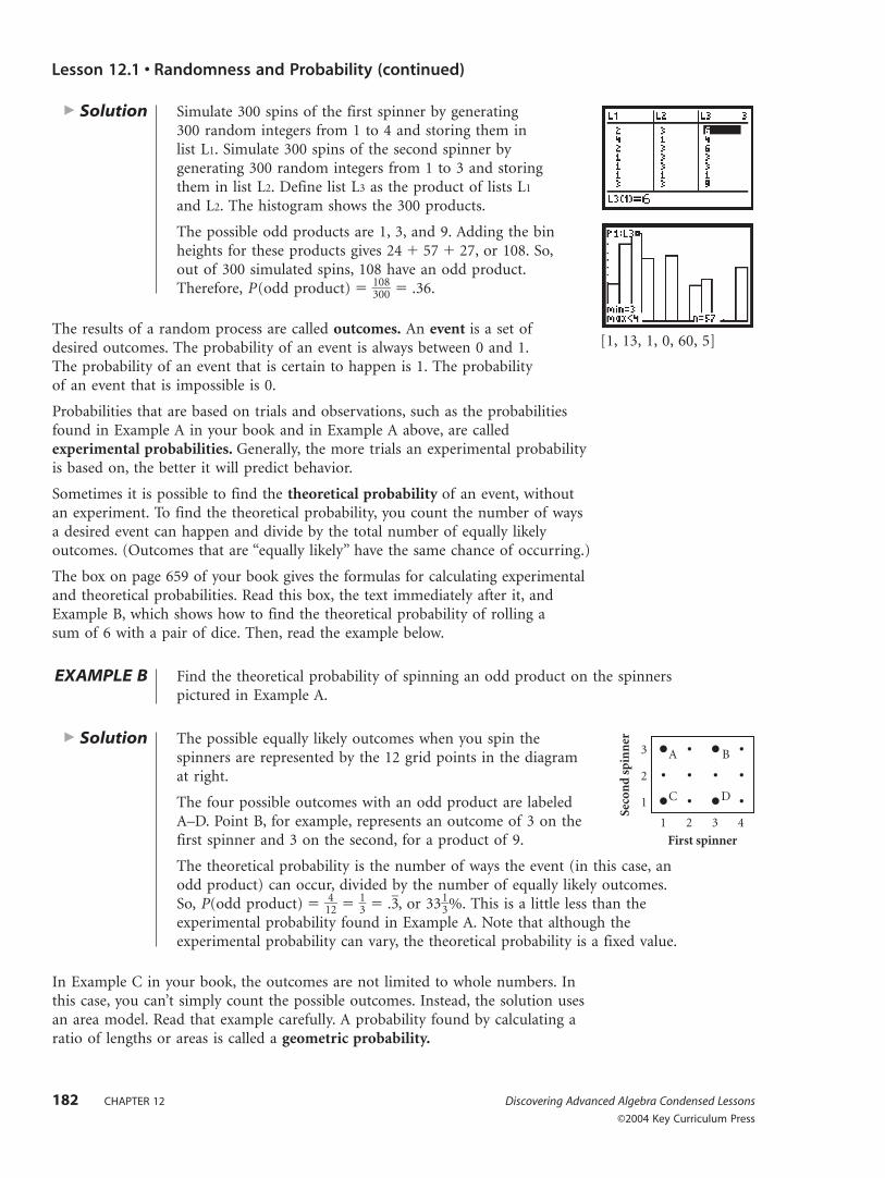
� Solution Simulate 300 spins of the first spinner by generating 300 random integers from 1 to 4 and storing them in list L1. Simulate 300 spins of the second spinner by generating 300 random integers from 1 to 3 and storing them in list L2. Define list L3 as the product of lists L1

and L2. The histogram shows the 300 products.

The possible odd products are 1, 3, and 9. Adding the bin heights for these products gives 24 � 57 � 27, or 108. So,out of 300 simulated spins, 108 have an odd product.Therefore, P(odd product) � �

13

00

80� � .36.

The results of a random process are called outcomes. An event is a set ofdesired outcomes. The probability of an event is always between 0 and 1.The probability of an event that is certain to happen is 1. The probability of an event that is impossible is 0.

Probabilities that are based on trials and observations, such as the probabilitiesfound in Example A in your book and in Example A above, are calledexperimental probabilities. Generally, the more trials an experimental probabilityis based on, the better it will predict behavior.

Sometimes it is possible to find the theoretical probability of an event, withoutan experiment. To find the theoretical probability, you count the number of waysa desired event can happen and divide by the total number of equally likelyoutcomes. (Outcomes that are “equally likely” have the same chance of occurring.)

The box on page 659 of your book gives the formulas for calculating experimentaland theoretical probabilities. Read this box, the text immediately after it, andExample B, which shows how to find the theoretical probability of rolling asum of 6 with a pair of dice. Then, read the example below.

EXAMPLE B Find the theoretical probability of spinning an odd product on the spinnerspictured in Example A.

� Solution The possible equally likely outcomes when you spin the spinners are represented by the 12 grid points in the diagramat right.

The four possible outcomes with an odd product are labeledA–D. Point B, for example, represents an outcome of 3 on thefirst spinner and 3 on the second, for a product of 9.

The theoretical probability is the number of ways the event (in this case, anodd product) can occur, divided by the number of equally likely outcomes.So, P(odd product) � �1

42� � �

13� � .3�, or 33�

13�%. This is a little less than the

experimental probability found in Example A. Note that although theexperimental probability can vary, the theoretical probability is a fixed value.

In Example C in your book, the outcomes are not limited to whole numbers. Inthis case, you can’t simply count the possible outcomes. Instead, the solution usesan area model. Read that example carefully. A probability found by calculating aratio of lengths or areas is called a geometric probability.

Seco

nd

sp

inn

er

3

2

1

2

A B

C D

3 4

First spinner

1

182 CHAPTER 12 Discovering Advanced Algebra Condensed Lessons

©2004 Key Curriculum Press

[1, 13, 1, 0, 60, 5]

DAA_CL_614_12.qxd 7/16/03 2:03 PM Page 182

L E S S O N

12.2CONDENSED

Counting Outcomes and Tree Diagrams


In this lesson, you

● Use tree diagrams to count outcomes and to find probabilities ofcompound events

● Compute probabilities of independent events and of dependent events

● Learn the multiplication rule for finding the probability of a sequenceof events

When determining the theoretical probability of an event, it can be difficult tocount outcomes. Example A in your book illustrates how making a tree diagramcan help you organize information. Read that example, and make sure youunderstand it.

In the tree diagram from Example A, each single branch represents a simpleevent. A sequence of simple events, represented by a path, is called acompound event.

Investigation: The Multiplication RuleWork through the investigation in your book, and then compare your results withthose below.

Step 1 Below is the tree diagram from Example A, part a, labeled withprobabilities. The probability of each simple event (getting a particular toy in abox) is .5. Because there are four equally likely paths, the probability of any onepath is �

14�, or .25. Notice that the probability of a path is the product of the

probabilities of its branches.

Step 2 The tree diagram from Example A, part b, labeled with probabilities, isshown on the next page. Note again that the probability of each path is theproduct of the probabilities of its branches. The sum of the probabilities of all thepaths is 1. The sum of the probabilities of the six highlighted paths is 6��2

17��, or �2

67�.

Toy 1

.5

.5

.5

.5

.5

.5

Toy 2

Toy 1

1st Box 2nd Box

Toy 2

Toy 1

Toy 2

a

b

c

d

P (Toy 1 followed by Toy 1) � .25




(continued)

DAA_CL_614_12.qxd 7/16/03 2:03 PM Page 183

Lesson 12.2 • Counting Outcomes and Tree Diagrams (continued)

Step 3

a. If there were four different toys, equally distributed among the boxes, thenthe probability of any particular toy in a particular box would be .25.

b. The probability that Talya finds a particular toy in one box does notinfluence the probability that she will find a particular toy in the next box.

c. There are 44, or 256 different equally likely outcomes. The outcome (Toy 3,followed by Toy 2, followed by Toy 4, followed by Toy 1) is one of theseoutcomes, so its probability is �2

156�, or about .004. You can also figure this

out by realizing that a complete tree diagram would have 256 paths andthe probability along each branch is .25. The specified outcome is one pathwith four branches, so its probability is (.25)(.25)(.25)(.25), or about .004.

Step 4 To find the probability of a path, multiply the probabilities of itsbranches.

1_3

1_3

1_3

1_3

1_3

1_3

1_3

1_3

1_3

1_3

1_3

1_3

1_3

1_3

1_3

1_3

1_3

1_3

1_3

1_3

1_3

1_3

1_3

1_3

1_3

1_3

1_3

3

2

3

1

2

1

1__27P (Toy 1, Toy 2, Toy 3) � � .037

1__27P (Toy 1, Toy 3, Toy 2) � � .037

1__27P (Toy 2, Toy 1, Toy 3) � � .037

1__27P (Toy 2, Toy 3, Toy 1) � � .037

1__27P (Toy 3, Toy 1, Toy 2) � � .037

1__27P (Toy 3, Toy 2, Toy 1) � � .037

Toy 11_3

Toy 21_3

Toy 31_3Toy 1

1_3

Toy 11_3

Toy 31_3

Toy 31_3 Toy 1

1_3

Toy 21_3

Toy 31_3

Toy 21_3

Toy 21_3



(continued)

DAA_CL_614_12.qxd 7/16/03 2:03 PM Page 184

Step 5 There are 24 paths that include all four toys. (For a sequence to havefour different toys, there are 4 possibilities for the first toy, then there are3 possibilities for the second toy, then 2 possibilities for the third toy, then1 possibility for the third. There are 4 � 3 � 2 � 1 such sequences.) So theprobability of getting a complete set is �2

2546�, or about .094.

In Example B in your book, a tree diagram showing every possible outcomewould be too much to draw. That example illustrates how, in such cases, you canoften make a tree diagram with branches of different possibilities. Read thatexample carefully. Below is another example.

EXAMPLE A Zak is working as a disk jockey at a party. To start the party, he puts three CDs inhis CD player. Disk 1 has 8 rock songs and 4 hip-hop songs. Disk 2 has 5 rocksongs and 5 hip-hop songs. Disk 3 has 3 rock songs and 12 hip-hop songs. IfZak randomly selects 1 song from Disk 1, then 1 from Disk 2, and then 1 fromDisk 3, what is the probability he will play exactly 2 hip-hop songs?

� Solution There are two branches for each CD, one for rock and one for hip-hop. Each branch islabeled with its probability. The highlighted paths are those that include exactly twohip-hop songs.

Find the probability of each path by multiplying the probabilities of its branches.

�23� � �

12� � �

45� � �1

45� �

13� � �

12� � �

45� � �3

40� �

13� � �

12� � �

15� � �3

10�

Now, add the probabilities of the three paths.

P(exactly 2 hip-hop songs) � �145� � �3

40� � �3

10� � �

13

30� � .43

R 1__5

H 4__5

R 1__5

H 4__5

R 1__5

H 4__5

R 1__5

H 4__5

R 1__2

H 1__2

R 1__2H 1__

3

1st CD 2nd CD 3rd CD

R 2__3

H 1__2



(continued)

DAA_CL_614_12.qxd 7/16/03 2:03 PM Page 185


In the preceding example, the probability that Zak plays a rock song from Disk 2is the same regardless of whether or not he plays a rock song from Disk 1. Theseevents are called independent, meaning that the occurrence of one event hasno influence on the occurrence of the other event. To find the probability of asequence of independent events, you simply multiply the probabilities of theevents. This is summarized in the box on page 671 of your book.

In part b of Example C in your book, the events are not independent. ReadExample C carefully, and make sure you understand it. Here is a similar example.

EXAMPLE B In Example A, suppose the host of the party tells Zak not to play two rock songsin a row. What is the probability Zak will play a rock song from Disk 2?

� Solution If Zak plays a rock song from Disk 1, then P(rock song from Disk 2) � 0 because hecannot play two rock songs in a row. If he plays a hip-hop song from Disk 1, thenP(rock song from Disk 2) � �

12�. There is a �

13� probability he will play a hip-hop

song from Disk 1, so the probability he plays a rock song from Disk 2 is �13� � �

12�, or �

16�.

When the probability of an event depends on the occurrence of anotherevent, the events are dependent. Independent and dependent events can bedescribed using conditional probability. If event A depends on event B, thenthe probability of A occurring given that B occurred is different from theprobability of A by itself. The probability of A given B is written P(AB). IfA and B are dependent, then P(AB) � P(A). If A and B are independent,then P(AB) � P(A).

In Example A, the events (rock on Disk 2) and (hip-hop on Disk 1) areindependent, so

P(rock on Disk 2 hip-hop on Disk 1) � P(rock on Disk 2)

In Example B, the events (rock on Disk 2) and (hip-hop on Disk 1) aredependent, so

P(rock on Disk 2 hip-hop on Disk 1) � P(rock on Disk 2)

72 of your book explains how you can use tree diagrams to break updependent events into independent ones. Read that text carefully, and then tryto make a similar diagram for the situation in Example B above. Then, read themultiplication rule.



DAA_CL_614_12.qxd 7/16/03 2:03 PM Page 186

L E S S O N

12.3CONDENSED

Mutually Exclusive Events andVenn Diagrams


In this lesson, you

● Learn the addition rule for mutually exclusive events

● Discover the general addition rule

● Use a Venn diagram to break non-mutually exclusive events into mutuallyexclusive events

Two events that cannot both happen are mutually exclusive. For example, passingthe history midterm and failing the history midterm are mutually exclusivebecause you can’t do both.

In Lesson 12.2, you saw how a tree diagram allows you to break down a sequenceof dependent events into a sequence of independent events. Similarly, you can usea Venn diagram to break down non-mutually exclusive events into mutuallyexclusive events. Here is an example.

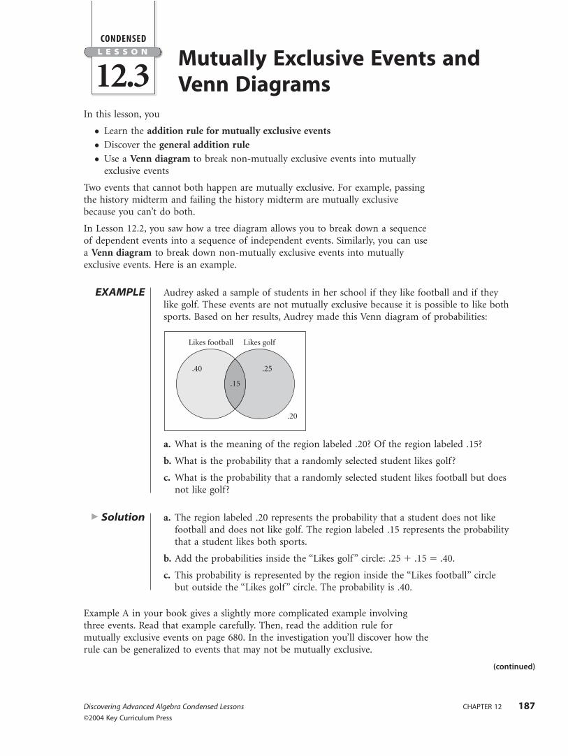
EXAMPLE Audrey asked a sample of students in her school if they like football and if theylike golf. These events are not mutually exclusive because it is possible to like bothsports. Based on her results, Audrey made this Venn diagram of probabilities:

a. What is the meaning of the region labeled .20? Of the region labeled .15?

b. What is the probability that a randomly selected student likes golf ?

c. What is the probability that a randomly selected student likes football but doesnot like golf ?

� Solution a. The region labeled .20 represents the probability that a student does not likefootball and does not like golf. The region labeled .15 represents the probabilitythat a student likes both sports.

b. Add the probabilities inside the “Likes golf” circle: .25 � .15 � .40.

c. This probability is represented by the region inside the “Likes football” circlebut outside the “Likes golf” circle. The probability is .40.

Example A in your book gives a slightly more complicated example involvingthree events. Read that example carefully. Then, read the addition rule formutually exclusive events on page 680. In the investigation you’ll discover how therule can be generalized to events that may not be mutually exclusive.

Likes football Likes golf

.40

.15

.25

.20

(continued)

DAA_CL_614_12.qxd 7/16/03 2:03 PM Page 187

Lesson 12.3 • Mutually Exclusive Events and Venn Diagrams (continued)

Investigation: Addition RuleWork through Steps 1–5 of the investigation in your book. Then, compare yourresults with those below.

Step 1 The events are not mutually exclusive because a student can take bothmath and science.

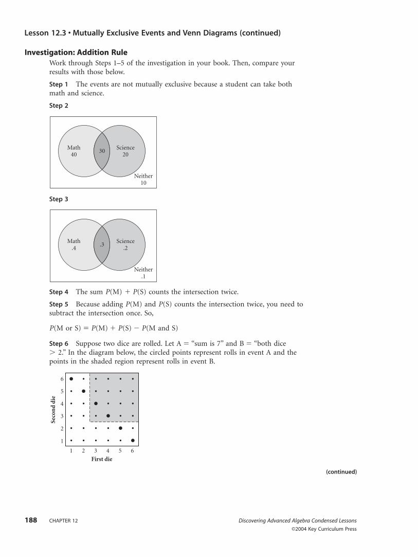
Step 2

Step 3

Step 4 The sum P(M) � P(S) counts the intersection twice.

Step 5 Because adding P(M) and P(S) counts the intersection twice, you need tosubtract the intersection once. So,

P(M or S) � P(M) � P(S) � P(M and S)

Step 6 Suppose two dice are rolled. Let A � “sum is 7” and B � “both dice� 2.” In the diagram below, the circled points represent rolls in event A and thepoints in the shaded region represent rolls in event B.

Seco

nd

die

6

5

4

3

2

1

2 3 4 5

First die

1 6

Math.4

.3Science

.2

Neither.1

Math40

30Science

20

Neither10



(continued)

DAA_CL_614_12.qxd 7/16/03 2:03 PM Page 188

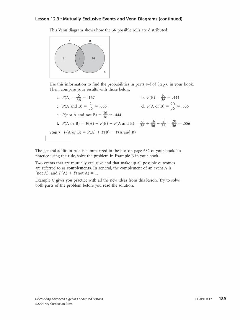
This Venn diagram shows how the 36 possible rolls are distributed.

Use this information to find the probabilities in parts a–f of Step 6 in your book.Then, compare your results with those below.

a. P(A) � �366� � .167 b. P(B) � �

13

66� � .444

c. P(A and B) � �326� � .056 d. P(A or B) � �

23

06� � .556

e. P(not A and not B) � �13

66� � .444

f. P(A or B) � P(A) � P(B) � P(A and B) � �366� � �

13

66� � �3

26� � �

23

06� � .556

Step 7 P(A or B) � P(A) � P(B) � P(A and B)

The general addition rule is summarized in the box on page 682 of your book. Topractice using the rule, solve the problem in Example B in your book.

Two events that are mutually exclusive and that make up all possible outcomesare referred to as complements. In general, the complement of an event A is(not A), and P(A) � P(not A) � 1.

Example C gives you practice with all the new ideas from this lesson. Try to solveboth parts of the problem before you read the solution.

A B

4 2 14

16

Lesson 12.3 • Mutually Exclusive Events and Venn Diagrams (continued)


DAA_CL_614_12.qxd 7/16/03 2:03 PM Page 189

L E S S O N

12.4CONDENSED

Random Variables andExpected Value


In this lesson, you

● Learn the meaning of random variable, geometric random variable, anddiscrete random variable

● Calculate the expected value of a random variable

At the end of basketball practice, the coach tells the players they can go home assoon as they make a free throw shot. Kate’s free throw percentage is 78%. Whatis the probability Kate will have to shoot only one or two times before she cango home?

The probability Kate will make her first shot is .78. From the diagram, you see that the probability she will miss her first shot and make her second shot is (.22)(.78), or .1716. To find the probability she will get to go home after only one or two shots, add the probabilities of the two mutually exclusive events:.78 � .1716 � .9516. The probability is about 95%.

Probabilities of success (in this case, making a basket) are often used to predictthe number of independent trials before the first success is achieved.

Investigation: “Dieing” for a FourComplete the investigation on your own, and then compare your results withthose below. If you don’t have your class’s data for Step 1, do 20 trials on yourown and find the mean.

Step 1 The results will vary, but the mean number of rolls should be about 6.

Step 2 Based on the experiment in Step 1, you would expect a 4 to come up onthe 6th roll.

Step 3 In this “perfect” sequence, a 4 comes up every 6 rolls.

Step 4 The probability of success on any one roll is �16�, and the probability of

failure is �56�. So,

P(rolling first 4 on 1st roll) � �16� � .167

P(rolling first 4 on 2nd roll) � ��56��

16�� 6

52� � �3

56� � .139

P(rolling first 4 on 3rd roll) � ��56��

56��

16��

56

2

3� � �22156� � .116

P(rolling first 4 on 4th roll) � ��56��

56��

56��

16��

56

3

4� � �1122956� � .096

Step 5 Using the pattern from Step 4, P(rolling first 4 on nth roll) � �56

n�

n

1�.

Step 6 The sum should be about 6. This is the average of the number of rolls itwill take to roll a 4.

Step 7 The sum you found in Step 6 should be close to your estimates inSteps 2 and 3.

Make .78

Miss .22

Make .78

Miss .22

1st Shot 2nd Shot

(continued)

DAA_CL_614_12.qxd 7/16/03 2:03 PM Page 191

Lesson 12.4 • Random Variables and Expected Value (continued)

A random variable is a numerical variable whose value depends on the outcomeof a chance experiment. In the investigation the random variable is the number ofrolls before getting a 4 on a die. The average value you found in Steps 2, 3, and 6is the expected value of this random variable. It is also known as the long-runvalue, or mean value.

The random variable in the investigation is a discrete random variable because itsvalues are integers. It is also called a geometric random variable, which means it isa count of the number of trials before something (a success or a failure) happens.

In Example A in your book, the random variable is the sum of two dice. Thisrandom variable is not geometric. Read Example A carefully, and make sure youunderstand it. The solution to part b demonstrates that to find the expectedvalue, you multiply each possible value of the random variable by the probabilityit will occur and then add the results. This is summarized in the “Expected Value”box on page 689 of your book.

Note that the random variable in the investigation had infinitely many possible

values (theoretically, the first 4 could occur on any roll), so the expected value

is the sum of a series—namely, ��

n�1

n � �56

n�

n

1�. The value you found in Step 6 of

the investigation was an estimate of the expected value. (It was the sum of the

first 100 terms.)

Example B in your book demonstrates that even if the random variable isdiscrete, its expected value may not be an integer. Read that example, and thenread the example below.

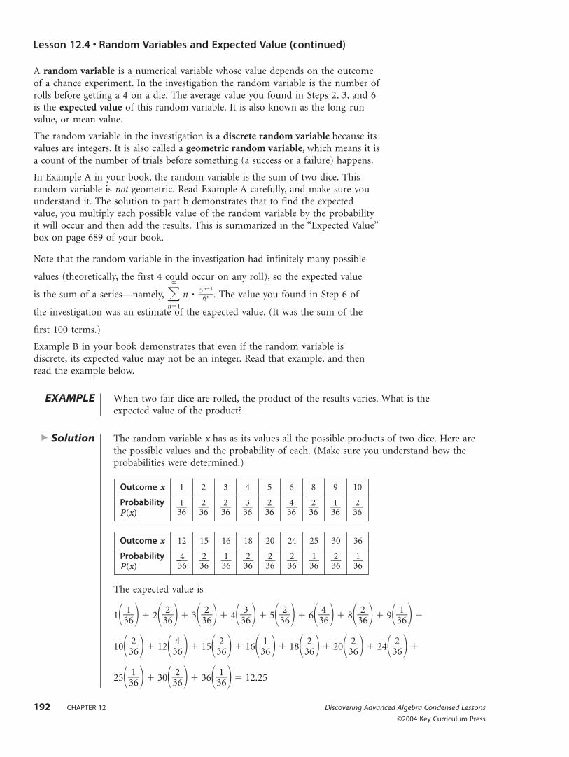
EXAMPLE When two fair dice are rolled, the product of the results varies. What is theexpected value of the product?

� Solution The random variable x has as its values all the possible products of two dice. Here arethe possible values and the probability of each. (Make sure you understand how theprobabilities were determined.)

The expected value is

1��316�� 2��3

26�� 3��3

26�� 4��3

36�� 5��3

26�� 6��3

46�� 8��3

26�� 9��3

16��

10��326�� 12��3

46�� 15��3

26�� 16��3

16�� 18��3

26�� 20��3

26�� 24��3

26��

25��316�� 30��3

26�� 36��3

16�� 12.25



Outcome x 1 2 3 4 5 6 8 9 10

�316� �3

26� �3

26� �3

36� �3

26� �3

46� �3

26� �3

16� �3

26�

ProbabilityP(x)

Outcome x 12 15 16 18 20 24 25 30 36

��346� �3

26� �3

16� �3

26� �3

26� �3

26� �3

16� �3

26� �3

16�

ProbabilityP(x)

DAA_CL_614_12.qxd 7/16/03 2:03 PM Page 192

In this lesson, you

● Learn the counting principle for counting outcomes involving a sequenceof choices

● Solve probability and counting problems involving permutations

● Use factorial notation to express the number of permutations of n objectstaken r at a time

Some probability situations involve a large number of possible outcomes. In thislesson, you will learn some shortcuts for “counting” outcomes.

Investigation: Order and ArrangeTry to complete the investigation in your book on your own. If you get stuck, orif you want to check your answers, read the results below.

Step 1 If n � 1 and r � 1, then there is one object, A, and one slot to fill. Inthis case there is only one thing you can do—put A in the slot.

If n � 2 and r � 1, then there are two objects, A and B, and one slot. In this casethere are two things you can do—put A in the slot or put B in the slot.

If n � 2 and r � 2, then there are two objects, A and B, and two slots. In thiscase there are two things you can do—put A in slot 1 and B in slot 2 or put Bin slot 1 and A in slot 2. You can represent these two possibilities as AB and BA.

Here are the possibilities for all the cases for n � 3. You can use a similar listingmethod to find the number of possibilities for n � 4 and n � 5.

n � 3 and r � 1: A, B, C (3 possibilities)

n � 3 and r � 2: AB, AC, BA, BC, CA, CB (6 possibilities)

n � 3 and r � 3: ABC, ACB, BAC, BCA, CAB, CBA (6 possibilities)

Here is the completed table at right:

Step 2 Possible patterns: The numbers inthe first row are consecutive integers. Inthe second row, the values increase byconsecutive even numbers (4 then 6 then8). In the third row, the numbers increaseby multiples of 18. In every column, theresults for r � n and r � n � 1 are thesame. This is because there is only oneway to place the last object.

There is a shortcut for counting the possibilities in the investigation. For example,suppose n � 4 and r � 3. Then there are four objects and three slots to fill. Thereare 4 choices of objects to go in the first slot. After the first slot is filled, there are3 choices left for the second slot. After the second slot is filled, there are 2 choicesleft for the third slot. So, the number of possibilities is 4 � 3 � 2 � 24. (If youhave trouble understanding why you must multiply, read the example about

L E S S O N

12.5CONDENSED

Permutations and Probability


(continued)

Number of items, n

n � 1 n � 2 n � 3 n � 4 n � 5

r � 1 1 2 3 4 5

r � 2 2 6 12 20

r � 3 6 24 60

r � 4 24 120

r � 5 120Nu

mb

er o

f sp

aces

,r

DAA_CL_614_12.qxd 7/16/03 2:03 PM Page 193

Lesson 12.5 • Permutations and Probability (continued)

choosing an outfit on page 695 of your book.) This shortcut, known as thecounting principle, is stated on page 695. Read Example A in your book, whichapplies the counting principle.

When a counting problem involves arrangements of objects in which each objectcan be used only once (as in the investigation), the arrangements are called“arrangements without replacement.” An arrangement of some or all of theobjects from a set, without replacement, is called a permutation. The notation nPris read “the number of permutations of n things chosen r at a time.” You calculate

nPr by multiplying n(n � 1)(n � 2) · · · (n � r � 1). Example B in your bookillustrates these ideas. Read that example, and then try the example below.

EXAMPLE Theo works as a dog walker. Today, he must walk Abby, Bruno, Coco, Denali,Emma, and Fargus.

a. In how many different orders can he walk the dogs?

b. Theo decides to choose the order at random. What is the probability he willwalk Abby first and Fargus last?

� Solution a. There are 6 choices for the first dog, 5 choices for the second dog, 4 choicesfor the third dog, and so on. The total number of possibilities is

6P6 � 6 � 5 � 4 � 3 � 2 � 1 � 720.

b. First, count how many orderings have Abby first and Fargus last. Draw six slotsto represent the dogs. There is 1 possibility for the first slot (Abby) and 1possibility for the last slot (Fargus).

_1 _ _ _ _ _1

There are then 4 choices for the second slot, then 3 choices for the third slot,then 2 choices for the fourth slot, then 1 choice for the fifth slot.

_1 _4 _3 _2 _1 _1

Using the counting principle, there are 1 � 4 � 3 � 2 � 1 � 1, or 24 orderingsin which Abby is first and Fargus is last. Thus, the probability Theo willwalk Abby first and Fargus last is �7

2240�, or �3

10�.

In part a of the example above, you can see that 6P6 is the product of all theintegers from 6 down to 1. The product of integers from n down to 1 is calledn factorial and is abbreviated n!. For example, 5! � 5 � 4 � 3 � 2 � 1 � 120.In general

nPn � n !

nPr � �(n �n!

r)!�

To learn about this in more detail, read the remainder of the lesson in your book.



DAA_CL_614_12.qxd 7/16/03 2:03 PM Page 194

L E S S O N

12.6CONDENSED

In this lesson, you

● Solve counting and probability problems involving combinations

● Discover how the number of combinations of n objects taken r at a time isrelated to the number of permutations of n objects taken r at a time

Suppose 8 players have entered a tennis tournament. In the first round, eachplayer must play each of the other players once. How many games will be playedin the first round? You might consider using the counting principle: There are8 choices for the first player, and then there are 7 choices left for her opponent,for a total of 8 � 7, or 56 possible pairings. However, notice that in this case theorder of the players does not matter. In other words, the pairing Player A vs.Player B is the same as Player B vs. Player A. Therefore, the total number ofgames is actually �8

2� 7�, or 28.

When you count collections of objects without regard to order, you are countingcombinations. In the tennis-tournament example, you found the number ofcombinations of 8 people taken 2 at a time. This is written 8C2. Although thereare 8P2 � 56 permutations of 8 people taken 2 at a time, there are only half thatmany combinations:

8C2 � �8P2

2� � �526� � 28

Read the text up to Example B in your book. Notice that the situation inExample A is very similar to the tennis-tournament situation above.

Example B in your book involves finding the number of combinations of4 people taken 3 at a time. Read that example carefully, and then read theexample below.

EXAMPLE Jason bought six new books. He wants to bring four of the books with him onhis summer trip. How many different combinations of four books can he take?

� Solution Because order doesn’t matter, you want to find the number of combinations of 6 bookstaken 4 at a time. However, first think about the number of permutations of 6 books(call them A–F) taken 4 at a time: 6P4 � 360. This number counts each combinationof 4 books 4!, or 24 times. For example, ABCD, ABDC, ACBD, ACDB, ADBC, ADCB,BACD, BADC, BCAD, BCDA, BDAC, BDCA, CABD, CADB, CBAD, CBDA, CDAB,CDBA, DABC, DACB, DBAC, DBCA, DCAB, and DCBA are counted separately becausethey are all different permutations. However, these 24 permutations represent only onecombination. Because each combination is counted 24 times, you must divide thenumber of permutations by 24 to get the number of combinations. So,

6C4 � �64P!4� � �

32640

� �15

There are 15 different combinations of 4 books Jason can take on his trip.

Combinations and Probability


(continued)

DAA_CL_614_12.qxd 7/16/03 2:03 PM Page 195

Lesson 12.6 • Combinations and Probability (continued)

Read the text in the “Combinations” box on page 705 of your book. To make sureyou understand the ideas, try to solve the problem in Example C before you readthe solution.

Investigation: Winning the LotteryRead Step 1 of the investigation in your book. If possible, talk to one of yourclassmates or to your teacher about what happened when your class simulatedplaying Lotto 47. Believe it or not, everyone in your class was probably seatedafter only three or four numbers were called!

Step 2 To find the probability that any one set of 6 numbers wins, first find thenumber of possible combinations. (Note that these are combinations because theorder does not matter.) There are 47 possible numbers, so the number of possiblecombinations is

47C6 � �6!(4747

�!

6)!� � 10737573

The probability that any one combination will win is �107317573�, or about

.0000000931.

If possible, complete the investigation using data from your class’s simulation.If not, use these made-up assumptions: There are six groups of 4 students in yourclass, your group generated a total of 100 combinations of six numbers, and thereare 1000 students in your school. The results below are based on theseassumptions.

Steps 3–6 Your group invested $100, and your class invested $600. Assuming the600 combinations are all different, the probability that someone in your class winsis �107

63070573�, or about .0000559.

Assuming each person in your school generated 25 combinations, for a total of25,000 combinations, the probability that someone in your school wins is �10

27530705073�,

or about .00233.

Step 7 If each of the 10,737,573 combinations were written on a 1-inch chipand the chips were laid end to end, then the line of chips would be about169 miles long (10737573 in. � 894797.75 ft � 169 mi).

Step 8 Answers will vary. One simple answer is that the probability of winningLotto 47 is the same as the probability of drawing your name randomly from ahat containing 10,737,573 different names (including yours, of course)!



DAA_CL_614_12.qxd 7/16/03 2:03 PM Page 196

L E S S O N

12.7CONDENSED

In this lesson, you

● Learn how the numbers of combinations are related to Pascal’s triangle

● Learn how the numbers of combinations are related to binomial expansions

● Use binomial expansions to find probabilities in situations involving twooutcomes

● Use information from a sample to make predictions about the population

At right are the first few rows of Pascal’s triangle. The triangle contains manydifferent patterns that have been studied for centuries. For example, notice that each number in the interior of the triangle is the sum of the two numbers above it. Take a few minutes to see what other patterns you can find.

In Lesson 12.6, you studied numbers of combinations. These numbers can befound in Pascal’s triangle. For example, the numbers 1, 5, 10, 10, 5, 1 in the sixthrow are the values of 5Cr:

5C0 � 1 5C1 � 5 5C2 � 10 5C3 � 10 5C4 � 5 5C5 � 1

In the investigation you will explore why the numbers of combinations appear inPascal’s triangle.

Investigation: Pascal’s Triangle and Combination NumbersComplete the investigation in your book, and then compare your results withthose below.

Step 1 5C3 � 10

Step 2 If Leora is definitely at the table, then two more students can sit at thetable. There are four students to choose the two students from, so the number ofpossible combinations is 4C2 � 6.

Step 3 If Leora is excluded, then three students must be chosen from the fourremaining students. The number of possible combinations is 4C3 � 4.

Step 4 If four students must be chosen from five students, then the number ofcombinations is 5C4 � 5. If Leora is definitely at the table, then the other threestudents must be chosen from the remaining four students. The number ofcombinations is then 4C3 � 4. If Leora is excluded, then the four students mustbe chosen from the four remaining students. The number of combinations is

4C4 � 1.

Step 5 5C3 � 4C2 � 4C3 and 5C4 � 4C3 � 4C4. In general,

nCr � n�1Cr�1 � n�1Cr

Step 6 In Pascal’s triangle, each entry (except a 1) is the sum of the two entriesabove it. The rth entry in row n � 1 is nCr, and the two entries above it are n�1Crand n�1Cr�1. Therefore, nCr � n�1Cr�1 � n�1Cr, which is precisely the pattern youfound in Step 5.

1

1 1

1 2 1

1 3 3 1

1 4 6 4 1

1 5 10 10 5 1

The Binomial Theorem andPascal’s Triangle


(continued)

DAA_CL_614_12.qxd 7/16/03 2:03 PM Page 197

Lesson 12.7 • The Binomial Theorem and Pascal’s Triangle (continued)

Pascal’s triangle is also related to expansions of binomials. For example, theexpansion of (x � y)3 is 1x3 � 3x 2y � 3xy 2 � 1y 3. Notice that the coefficients ofthe expansion are the numbers in the fourth row of Pascal’s triangle. Why are thenumbers in Pascal’s triangle equal to the coefficients of a binomial expansion?The numbers in Pascal’s triangle are values of nCr, so you can restate this questionas, Why are the coefficients of a binomial expansion equal to values of nCr? Toexplore this question, read Example A in your book and the text immediatelyfollowing it. Then, read the statement of the Binomial Theorem on page 712.

Example B in your book shows how you can use a binomial expansion to find theprobabilities of outcomes that are not equally likely. Read that example, followingalong with a pencil and paper, and then read the example below.

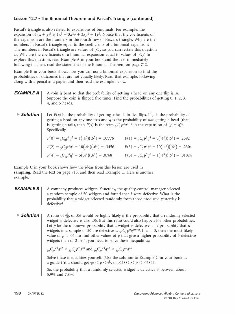
EXAMPLE A A coin is bent so that the probability of getting a head on any one flip is .4.Suppose the coin is flipped five times. Find the probabilities of getting 0, 1, 2, 3,4, and 5 heads.

� Solution Let P(x) be the probability of getting x heads in five flips. If p is the probability ofgetting a head on any one toss and q is the probability of not getting a head (thatis, getting a tail), then P(x) is the term 5Cx pxq5�x in the expansion of (p � q)5.Specifically,

P(0) � 5C0p0q5 � 1�.40��.65� � .07776 P(1) � 5C1p1q4 � 5�.41��.64� � .2592

P(2) � 5C2p2q3 � 10�.42��.63� � .3456 P(3) � 5C3p3q2 � 10�.43��.62� � .2304

P(4) � 5C4 p4q1 � 5�.44��.61� � .0768 P(5) � 5C5p5q0 � 1�.45��.60� � .01024

Example C in your book shows how the ideas from this lesson are used insampling. Read the text on page 713, and then read Example C. Here is anotherexample.

EXAMPLE B A company produces widgets. Yesterday, the quality-control manager selecteda random sample of 50 widgets and found that 3 were defective. What is theprobability that a widget selected randomly from those produced yesterday isdefective?

� Solution A ratio of �530�, or .06 would be highly likely if the probability that a randomly selected

widget is defective is also .06. But this ratio could also happen for other probabilities.Let p be the unknown probability that a widget is defective. The probability that nwidgets in a sample of 50 are defective is 50Cn pnq50�n. If n � 3, then the most likelyvalue of p is .06. To find other values of p that give a higher probability of 3 defectivewidgets than of 2 or 4, you need to solve these inequalities:

50C3p3q47 � 50C2 p2q48 and 50C3p3q47 � 50C4 p4q46

Solve these inequalities yourself. (Use the solution to Example C in your book asa guide.) You should get �1

17� � p � �5

41�, or .05882 � p � .07843.

So, the probability that a randomly selected widget is defective is between about5.9% and 7.8%.



DAA_CL_614_12.qxd 7/16/03 2:03 PM Page 198

LESSON - Prek 12math.kendallhunt.com/documents/daa1/CondensedLessonPlans/DAA_CLP...Solution The...

Documents

Transcript of LESSON - Prek 12math.kendallhunt.com/documents/daa1/CondensedLessonPlans/DAA_CLP...Solution The...