Lesson 9: Advanced M/G/1 Methods and Examples Giovanni Giambene Queuing Theory and...

Lesson 9: Advanced M/G/1 Methods and ExamplesGiovanni Giambene

Queuing Theory and Telecommunications: Networks and Applications2nd edition, Springer

All rights reserved

Slide supporting material

© 2013 Queuing Theory and Telecommunications: Networks and Applications – All rights reserved


M/G/1 with Different Imbedding Options and M/G/1 with Differentiated Service Times


Advanced ‘M’/G/1 cases


taking into account:

Synchronization effects for the service of arrivals occurring at an empty queue

Compound arrivals

Batched service

Imbedding optionsMessage level(mean msg delay, Tm)Message completion instants

Packet level(mean numberof packets, Np)

Packet completion instants

End of the slot

End of the frame



These ‘M’/G/1 cases are modeled by generalized difference equations as:

The above is a symbolic difference equation presented to introduce new concepts, but not actually corresponding to a given queuing system.

0 if,

1 if,0,max

1

11

ii

iiii na

nabnn

batched service (deterministic or random) per imbedding interval if b > 1

service differentiation if D > 0


‘M’/G/1 Queue with Different Imbedding Options

Let us refer to a queue with a compound Poisson arrival process. Different imbedding options are available, also depending on the presence of an output Time Division Multiplexing (TDM)/TDMA service.

1. Imbedding at the end of the packet transmission time to study the statistics of the buffer occupancy (like MAC layer performance). This study requires to adopt the service differentiation approach. Notation: M[G]/D/1.

2. In a TDM output case, we can also imbed the system at the end of the output slot, thus avoiding any service differentiation issue. Notation: M[G]/D/1.

message arrival

time

packets


‘M’/G/1 Queue with Different Imbedding Options

3. In a TDMA case and asynchronous multiplexing, we can imbed the system at the end of the frame with b slots, thus having a batched service since we can service up to b packets per frame. Notation: M[G]/D[b]/1.

4. Imbedding at the end of the message transmission time to study the message delay distribution (like layer 3 performance). Notation: M/G/1. We use the Pollaczek-Khinchin formula.

In the above cases #1, #2, #3, operating at the packet level, the arrival process is not Poisson, and the Kleinrock principle is not applicable due to the simultaneous arrival of the packets of a message. Hence, the ‘M’/G/1 solution depends on the imbedding points.

Instead, in the above case #4, the arrival process is Poisson and we can apply the PASTA property.

message arrival

time

packets


Let us Re-examine Exercise #2 of Lesson #7 We consider a transmission line with a buffer (i.e., we have

a single-server queue) where messages arrive according to a Poisson process with mean arrival rate l.

The arrival process and the transmission one are continuous-time.

All the packets of the same message arrive simultaneously: bulk arrival process.

A message is formed of a random number l of packets, each requiring a time T to be transmitted. Message lengths are iid.

Let L(z) denote the PGF of the message length in packets that also corresponds to the PGF of the message transmission time in T time-units.

l

L(z)

message arrival

time

packets

Note that both inputs and outputs are unslotted. We have thus 2 different imbedding options (cases #1 and #4).


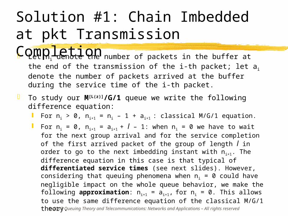
Solution #1: Chain Imbedded at pkt Transmission Completion Let ni denote the number of packets in the buffer at the end of

the transmission of the i-th packet; let ai denote the number of packets arrived at the buffer during the service time of the i-th packet.

To study our M[L(z)]/G/1 queue we write the following difference equation: For ni > 0, ni+1 = ni – 1 + ai+1 : classical M/G/1 equation.

For ni = 0, ni+1 = ai+1 + l – 1: when ni = 0 we have to wait for the next group arrival and for the service completion of the first arrived packet of the group of length l in order to go to the next imbedding instant with ni+1. The difference equation in this case is that typical of differentiated service times (see next slides). However, considering that queuing phenomena when ni = 0 could have negligible impact on the whole queue behavior, we make the following approximation: ni+1 = ai+1, for ni = 0. This allows to use the same difference equation of the classical M/G/1 theory.

In order to apply the M/G/1 theory we need to compute A(z) that represents the PGF of the number of packets arrived at the buffer in the service time of a packet (time T).


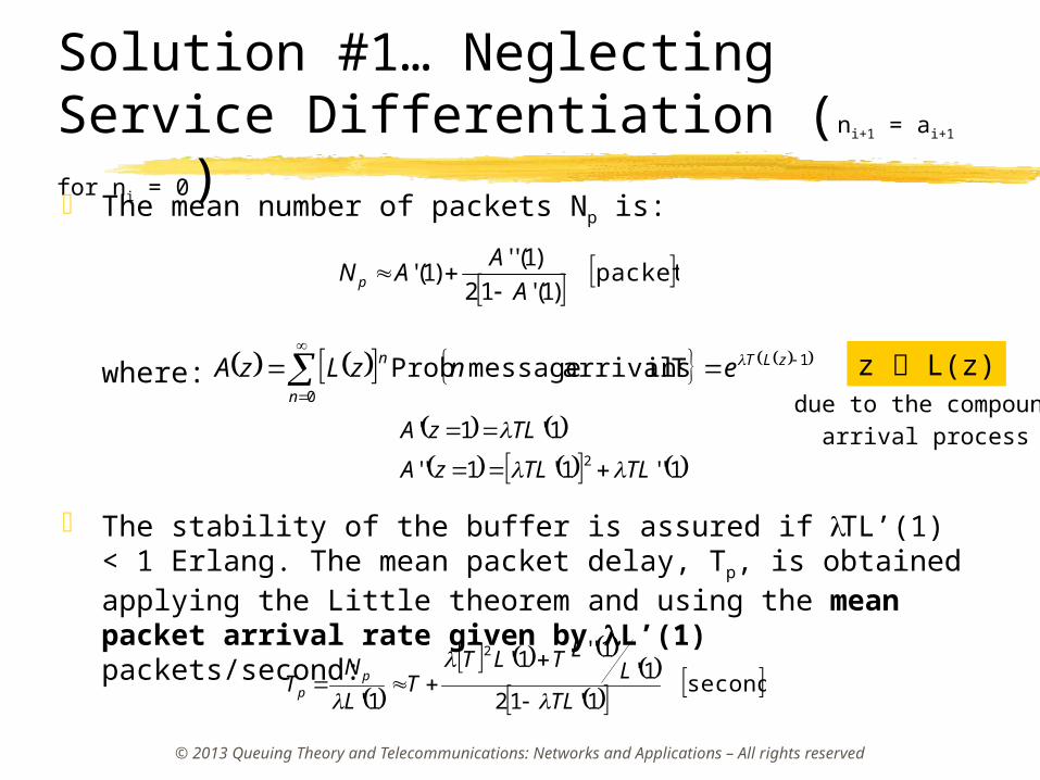
Solution #1… Neglecting Service Differentiation (ni+1 = ai+1 for ni = 0)

The mean number of packets Np is:

where:

The stability of the buffer is assured if lTL’(1) < 1 Erlang. The mean packet delay, Tp, is obtained applying the Little theorem and using the mean packet arrival rate given by lL’(1) packets/second:

1

0

Tin arrivals message Prob

zLT

n

n enzLzA

packets)1('12

)1('')1('

A

AAN p

1''1'1''

1'1'2 TLTLzA

TLzA

seconds1'12

1'1''1'

1'

2

TLL

LTLTT

L

NT pp

z L(z)due to the compound

arrival process


Solution #1b with Differentiated Service Times (ni+1 = ai+1 + D for ni = 0)

The chain is again imbedded at the end of packet transmission:ni+1 = ni – 1 + ai+1, if ni 0,

ni+1 = ai+1*, if ni = 0 where ai+1* = ai+1 + w and w = l – 1 (since ai+1* > ai+1 , this case is as if the service time was longer when the buffer is empty as with ‘differentiated service times’). In terms of PGFs, A(z) does not change with respect to the previous example and W(z) = L(z)/z.

We need to solve the new difference equation in the z-domain and to compute the derivatives of the PGF P(z) at z = 1. We have:

cells1'12

1''1'

1'2

1''

A

AA

L

LN p

Classical M/G/1

terms (as in solution #1)

Additional term due todifferentiation dependingon the message length

statistics; this term disappearsif the messages are formed of

a single packet L(z) = z.

Note: Random variable L PGF L(z)Random variable –1 PGF z-1


Solution #2: Chain Imbedded at msg Transmission Compl.

Let ni denote the number of messages in the buffer at the end of the transmission of the i-th message; let ai denote the number of messages arrived at the buffer during the service time of the i-th message.

We can write the following difference equation of the classical M/G/1 type: For ni > 0, ni+1 = ni – 1 + ai+1

For ni = 0, ni+1 = ai+1.

In order to apply the M/G/1 theory we need to compute A(z) that represents the PGF of the number of messages arrived at the buffer in the service time of a message.

1 zTeLzA 1'1''1''

1'1'2 LLTzA

TLzA

This composition is exactly the opposite of that used for solution #1

Of course this case can be solved by directly

applying the Pollaczek-Khinchin formula. We have

however computed A(z) to compare to that of

solution 1

This is the same case ofExercise #2 in Lesson #7 !


Solution #2…

Let Nm denote the mean number of messages in the queue:

The stability condition is lTL’(1) < 1 Erlang. Since the mean arrival rate of messages is l, we apply the Little theorem

to derive the mean message delay Tm:

Let us consider messages with modified-geometric distribution {so that L’’(1)=2[L’(1)]2-2L’(1)}. Hence, the mean message delay Tm results as:

Under the approximation considered in case #1 for the derivation of Tp, we can prove that Tp Tm.

pkts1'12

1'1''1'

)1('12

)1('')1('

2

TL

LLTTL

A

AANm

s1'12

1'1''1'

2

TL

LLTTL

NT mm

s1'12

1'1'21'

22

TL

LLTTLTm


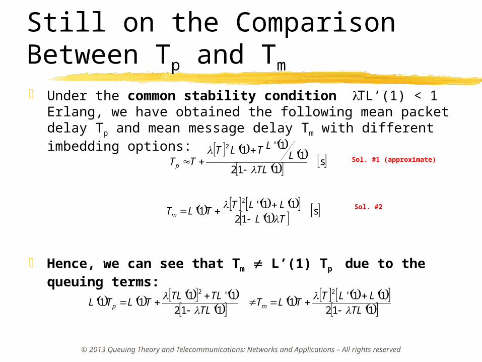
Still on the Comparison Between Tp and Tm

Under the common stability condition lTL’(1) < 1 Erlang, we have obtained the following mean packet delay Tp and mean message delay Tm with different imbedding options:

Hence, we can see that Tm L’(1) Tp due to the queuing terms:

s1'12

1'1''1'

2

TL

LLTTLTm

s1'12

1'1''1'2

TLL

LTLTTTp

1'12

1'1''1'

1'12

1''1'1'1'

22

TL

LLTTLT

TL

TLTLTLTL mp

Sol. #2

Sol. #1 (approximate)


Still on the Comparison Between Tp and Tm

Under the common stability condition lTL’(1) < 1 Erlang, we have obtained the following mean packet delay Tp and mean message delay Tm with different imbedding options:

Hence, we can see that Tm L’(1) Tp due to the queuing terms:

s1'12

1'1''1'

2

TL

LLTTLTm

s1'12

1'1''1'2

TLL

LTLTTTp

1'12

1'1''1'

1'12

1''1'1'1'

22

TL

LLTTLT

TL

TLTLTLTL mp

Sol. #2

Sol. #1 (approximate)

To remove the approximation we should add a term L’’(1)/[2lL’(1)2].


M/G/1 Queue with Feedback or Randomly-Available Server Let us consider a queue receiving packets according to a Poisson process

with mean rate l. Each packet needs a time T to be transmitted (deterministic service). Service time is slotted (synchronized) with duration T. When a packet is transmitted, with probability 1-p it is sent instantaneously back to the queue (due to an error - ARQ scheme).

We imbed the queue at the slot end instants.

Let ni denote the number of packets in the

queue at the end of the i-th slot;

Let ai denote the number of packets arrived at

the queue during the i-th slot.

Variable X representing the service is a Bernoulli random variable equal to 1 with probability p and equal to 0 with probability 1-p. X(z) = zp+ 1-p. E[X] = p.

We can thus write the following difference equation modeling this queue:

p

1-p

+l

0 if,

1 if,

1

11

ii

iiii na

naXnn

slot slot slot











p

1-p

+l

0 if,

1 if,

1

11

ii

iiii na

naXnn

slot slot slot

This model is equivalent to consider that the output server is available in a slot to send a packet with probability p and unavailable with probability 1-p (insensitivity property).











p

1-p

+l

0 if,

1 if,

1

11

ii

iiii na

naXnn

slot slot slot

This approach is correct, but does not permit to model the synchronization delays in the service of packets arrived at an empty buffer. Otherwise, we could consider a different model of this system without slots for output transmissions: transmissions are continuous-time. We could thus avoid synchronization issues. In this case, we should imbed the study at the packet transmission end, thus using again the classical M/G/1 difference equation.


M/G/1 Queue … (cont’d)

We solve the difference equation by transforming in the z-domain and using the same method adopted for the classical M/G/1 study.

We obtain the following results for the PGF of the packets in the buffer, P(z), and the mean number of packets in the queue:

where the stability condition is now A’(1) = lT < p Erl.

Note: Random variable X PGF X(z)Random variable –X PGF X(z-1)

)(1

)(1

)(1

)(101

1

0 zApzpz

zAzpP

zAzX

zAzpPzP

10 ,

1'

zTezAp

ApP

pkts

)1('2

)1(''

)1('

)1('1)1('

Ap

A

Ap

ApAN

Note that for p =1 the feedback is eliminated and this expression yieldsthe classical M/G/1 result.

The mean packet delay T can be obtained by applying the Little theorem to the whole queuing system: T = N/l


Thank you!

[email protected]

Lesson 9: Advanced M/G/1 Methods and Examples Giovanni Giambene Queuing Theory and...

Documents

Transcript of Lesson 9: Advanced M/G/1 Methods and Examples Giovanni Giambene Queuing Theory and...