LESSON 16

Spreadsheets

FormattingWorksheet Data

LEARN

Changing The appearance of your worksheet is important. The informationthe should be as clear and as attractive as possible. Worksheets can

learance contain a lot of data. You want to be able to see what's important

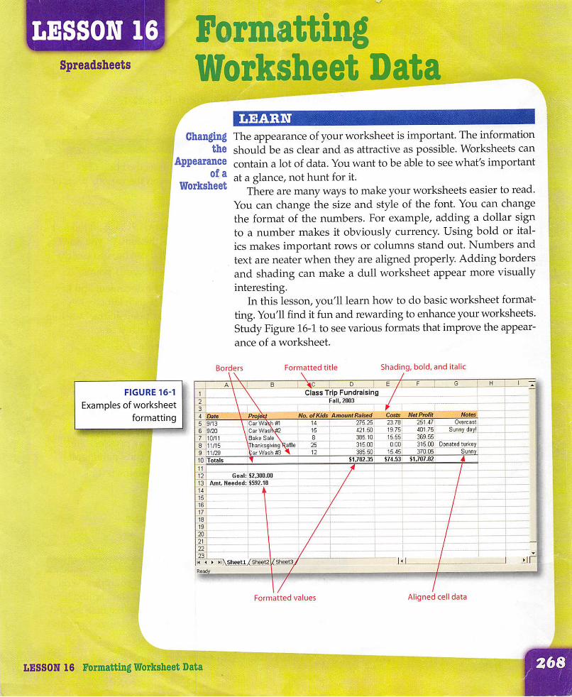
® at a glance, not hrmt for it.Worksheet are many ways to make your worksheets easier to read.You can change the size and style of the font. You can changethe format of the numbers. For example, adding a dollar signto a number makes it obviously currency. Using bold or italics makes important rows or columns stand out. Numbers andtext are neater when they are aligned properly. Adding bordersand shading can make a dull worksheet appear more visuallyinteresting.

In this lesson, you'll learn how to do basic worksheet formatting. You'll find it fun and rewarding to enhance your worksheets.Study Figure 16-1 to see various formats that improve the appearance of a worksheet.

Borders Formatted title Shading, bold, and italic

FIGURE 16-1

Examples of worksheet

formatting

Class Trip FundraislngFall. 2QQ3

fMPmSt NotesNo. ofKids AmountRalsed251.47

401.75

369.55

315.00 Donated turkey370.05 Sunriy

275.25

421.50

385.10

315.00

385.50

CarWa\h#1

Car Was

Baka Sale

Thanksgiving \afflaar Wash #3

10 Totals $1,707.82$1,782.35

Goal: $2,300.00

AmL Needed: $592.18

^Sheetl/Sheet2

Aligned cell dataFormatted values

LESSON 16 Formatting Worksheet Data

Microsoft Excel ^

Changing FontsThe worksheet's default font is 10-point Arial. You can change both the font and its sizeby using the Formatting toolbar.

To change the font:

1. Select the cell(s) you want to change.

2. Click the down arrow next to the Font box on the Formatting toolbar.A drop-down menu appears.

3. Click the desired font.

To change the font size:

1. Select the cell(s) to change.

2. Click the down arrow next to the Font Size box on the Formatting toolbar.A drop-down menu appears.

3. Click the desired font size.

w

ChangeFonts

EXCEL TIP

A worksheet's title

usually has thelargest font.

USSSON 16 Formatting Worksheet Data

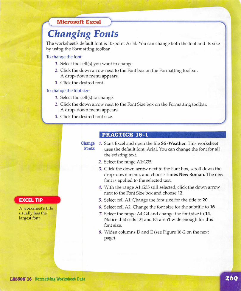
PRACTICE 16-1

1. Start Excel and open the file SS-Weather. This worksheetuses the default font, Arial. You can change the font for allthe existing text.

2. Select the range A1:G35.

3. Click the down arrow next to the Font box, scroll down the

drop-down menu, and choose Times New Roman. The newfont is applied to the selected text.

4. With the range A1:G35 still selected, click the down arrownext to the Font Size box and choose 12.

5. Select cell Al. Change the font size for the title to 20.

6. Select cell A2. Change the font size for the subtitle to 16.

7. Select the range A4:G4 and change the font size to 14.Notice that cells D4 and E4 aren't wide enough for thisfont size.

8. Widen columns D and E (see Figure 16-2 on the nextpage).

FIGURE 16-2

Changing

worksheet fonts

Microsoft Excel - SS-Vfealher [Reod-Only]

0^ Cdt Ifjew Insert Format lods Qata tfndow Help TTxl^ .O » r. . H "a>^ - 0■ , 1

: Times New Romen « 14 • B 7 u W9m 'ji i^iP- _■p » A 1E4 fit Wind Speed E

A B C D F 1 0 1 H 1 1 „ J1 J 1 K-r®

Weather Almanac ]1 1

2 Month of October3

Isunrise4 Day Sgh Low Precipitation jWind Speed I Sunset :!

5 1 •g

6 2 i i7 3.

. 16 4: i ] 19

1

•

10 6f11 1\12 8:13 9

14 10' ! 1 I ] i

15 11——• < ' ■—1 ..... -j

1

16 " 'l2i '17 13! 1 1 11S 14' ; ! 1 -i*

H 4 » H\Weather/Sheet2/She8t3/ U! 1Reedy

mmrnmmmt

EXCEL TIP

In general, it is betternot to mix fonts in thesame worksheet.

9. Select cell A1 again. Try out other fonts. Some are verydramatic. Change cell A1 back to 20-point Times NewRoman when you finish.

10. Leave the file open.

Microsoft Excel ^

Applying Bold^ Italic^ and UnderlinesYou can apply bold, italic, and underlines to worksheet cells by using buttons onthe Formatting toolbar. You can remove the formatting by selecting the cell(s) andclicking the button again. Table 16-1 describes the buttons you can use to formatworksheet cells.

TABLE 16-1 Toolbar Buttons for Bold, Italic, and Underline

Button Format

a BoldApplies bold to selected cells.

0 ItalicApplies italic to selected cells.

a UnderlineApplies underlines to selected cells.

J

LI880H 16 Formatting Worksheet Data

PRACTICE 16-2

Use Bold}Italic, andUnderline

1. With the SS-Weather file still open, select the range A1:A2.

2. Click the Bold button 0 on the Formatting toolbar to applybold to the cells.

3. Select the range A4:G4 and apply bold. Cells can have morethan one attribute.

With the range still selected, click the Italic button 0 toapply italic. Notice that the columns are too small for someof the cells you changed.

5. Widen columns D through F.

6. Select the range A4:G4 and click the Underline button L5.button to underline the text.

7. Click the Print Preview button to see how the underlines

will appear when you print the worksheet. (Click Zoom onthe menu bar if the image is too small.)

FIGURE 16-3

Previewing bold, italic,

and underlines

□ Microsoft Excel • SS-Weather [Read-Only]I' Zoom l| Piir^,,, j S»fa<>— j ttarQins | Papa BreakPreyiewj gose | tt*

Weather AlmanacMonth of October

Day Hieh12

34

56

7

89

1011

1213

14

Lav Preetdiadm Wind Speed Sunrise Sunset

of i

8. Close Print Preview. You remove an attribute by using thesame button.

9. With the range A4:G4 still selected, click the Underlineagain to remove the underlines.button u

10. Key your name in cell Fl.11. Save the file as [your initials]Vracticel6-2. Print the

worksheet and close the workbook. Leave Excel open.

USSOH 16 Formatting Worksheet Data

Microsoft Excel >Formatting ValuesYou can apply formatting to worksheet values by using buttons on the Formatting toolbar or menu bar. You can add dollar signs, percent signs, commas, and decimal placesto your numbers. You can also format dates.

To format numbers in selected cells by using the menu bar:

1. Open the Format menu and choose Cells. The Format Cells dialog box appears.

2. Click the Number tab if it is not already displayed.

3. Click the desired Category. For Number, Currency, and Percentage, you canselect the number of Decimal places. For Date, you select a date format in theType box. Click OK.

Table 16-2 describes the buttons on the Formatting toolbar you can use to format values.

TABLE 16-2 Toolbar Buttons for Formatting Values

$ CurrencyApplies the accounting style currency format.

% PercentApplies the percent style.

j CommaAdds commas and decimal places.

l+.o1 ,00 Increase Decimal

Adds decimal places In a number.

.00-¥.0 Decrease Decimal

Reduces the decimal places In a number.

x.9m

PRACTICE 16-3

Format 1. Open the file SS-FundRaising. The dates and values in thisValues worksheet are unformatted. Formulas automatically calculate

the totals. (You'll learn more about formulas in the next lesson.)

2. Click cell AlO and key the following information acrossrow 10:

12/13/2003 Wreath Sale 23 653 125

3. Click cell Dll. Open the Format menu and choose Cells. TheFormat Cells dialog box appears. Click the Number tab if itis not already displayed.

U58SON 16 Formatting Worksheet Data

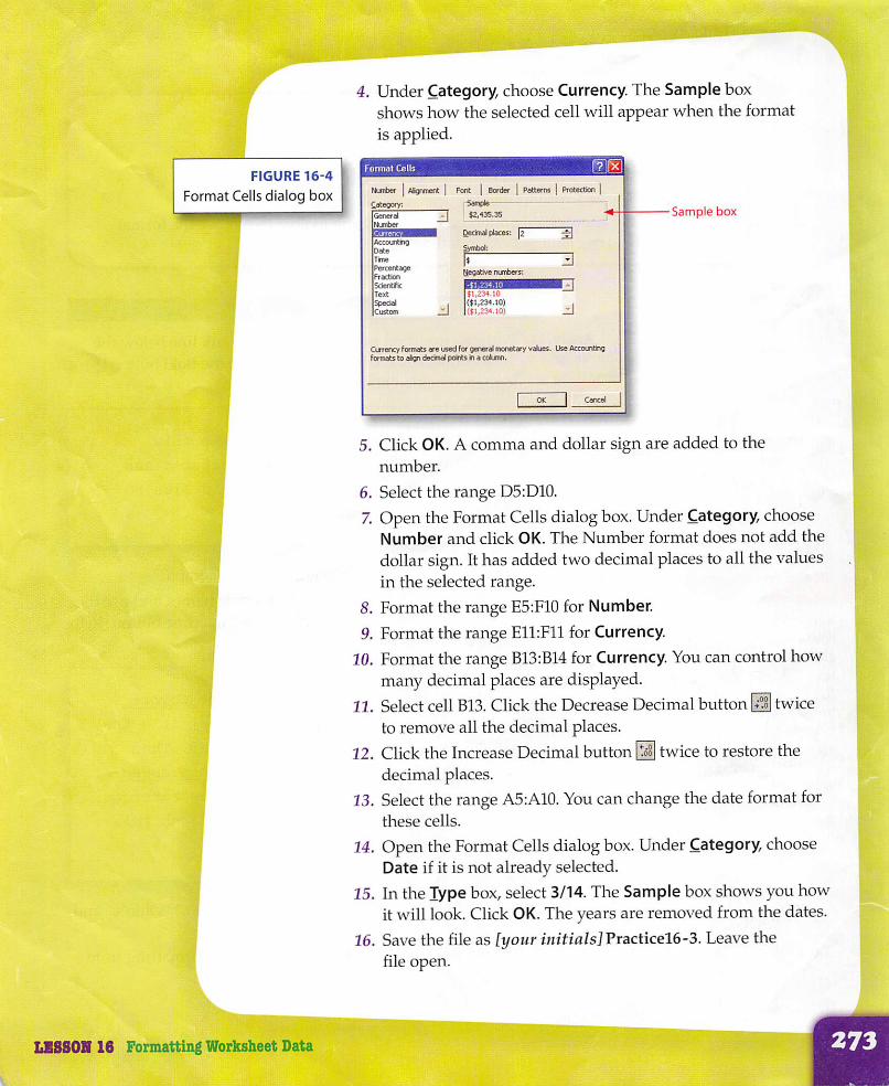
4. Under Category, choose Currency. The Sample boxshows how the selected cell will appear when the formatis applied.

FIGURE 16-4

Format Ceils dialog boxNwrter ] AigmenC

Categorv:

Pactems

Sample box$2,435.35GeneralNumbs

Qieonal places: hAccotrtingDate

Tine

Percentage

Fraction

5cientficText

SpecialCustom

Synbol:

Negative runbers:

$1,234.10{$1,234.10)($1,234.10)

Currency Formats are used for general nnnAary values. UseAccouitngFormats to aign dednal points it a cokiiin.

Ki

5. Click OK. A comma and dollar sign are added to thenumber.

6. Select the range D5:D10.

7. Open the Format Cells dialog box. Under Category, chooseNumber and click OK. The Number format does not add the

dollar sign. It has added two decimal places to all the valuesin the selected range.

8. Format the range E5:F10 for Number.

9. Format the range E11:F11 for Currency.

10. Format the range B13:B14 for Currency. You can control howmany decimal places are displayed.

11. Select cell B13. Click the Decrease Decimal button § twiceto remove all the decimal places.

12. Click the Increase Decimal button @1 twice to restore thedecimal places.

13. Select the range A5:A10. You can change the date format forthese cells.

14. Open the Format Cells dialog box. Under Category, chooseDate if it is not already selected.

15. In the lype box, select 3/14. The Sample box shows you howit will look. Click OK. The years are removed from the dates.

16. Save the file as [your initials] Vraciicel6-3. Leave thefile open.

LESSOSf 16 Formatting Worksheet Data

--r

Microsoft Excel ^

Aligning Cell DataInformation can be placed on the left or right side of the cell or centered in the cell. Youcan also merge selected cells and center data across the merged cells. The resultingmerged cells contain only the left-most data in the selection, which is centered in themerged cells.

Table 16-3 describes the buttons on the Formatting toolbar you can use to align cellcontents.

TABLE 16-3 Toolbar Buttons for Cell Alignment

Aligns contents of selected cell on the left.Align Left

_ Align RightAligns contents of selected cell on the right.

CenterCenters contents in the center of selected cell.

haH Merge and CenterMerges two or more selected adjacent cells to create asingle cell.

Align CellData

PRACTICE 16-4

Aligning text and numbers below the column headings makesthem easier to read.

1. With the file [your mitials]Fracticel6-3 still open, select therange A5:A10. YouTl left-align these dates. Dates are treatedas values. By default, values are always aligned on the right.

2. Click the Align Left button to align the dates with thecolumn heading.

3. Select the range C5:C10. Click the Center button 8 to centerthe numbers below the column heading.

4. Select the range D4:F4. Click the Align Right button 8 toalign the headings on the right side of the cells, above thenumbers. By default, text is always aligned on the left.

5. Align the range A13:A14 to the right.

6. Align the range B13:B14 to the left. Now the numbers andlabels for this information appear next to each other.

7. Select the range A1:G1. YouTl merge and center the cells inthis range.

LI8S0N 16 Formatting Worksheet Data

8. Click the Merge and Center button [B]. The selected range iscombined into a single cell. The resulting merged cell containsonly the left-most data, which is centered in the merged cell.

9. Select the range A2:G2 and click the Merge and Center!. The subtitle is merged and centered acrossbutton

FIGURE 16-5

Aligning worksheet data

the range.

10. Click cell A3. Notice that the gridlines for the merged cellsshow only a single cell that extends to column G.

•Merged cells

A 1 B C D E 1 F G H 1 T*

Class Trip Fundralsing? Fall, 2003

•3 14 No. ofKids Amount Raised Costs Net Profit Notes 'iS 9/13 CarWashiM 14 275.25 23.78 251.47 Overcast

R 9/20 Car Wash ffi 15 421.50 19.75 401.75'Sunny dayl

7 10/11 Bake Sale 6 385.10 15.55 369.55

R 11/15 iThanksglving Raffle11/29 ^CarWash#3

25 315.00: O.GO 315.IX):Oonated turkey

9 12 385.50! 15.45- 370.05'Sunny

in 12/13 Wreath Sale 23 653.00' 125.00 528.(X)

11 Totals $2,43535 $19933 $233532

1?

13 Goal; $23004)014 AmL Needad: $64.10

"15^ "r ! i : I

16 - --C: ■ i- !■

11. Preview the worksheet to see how the alignments willappear when printed. The alignments can look differentwithout the gridlines.

12. Save the file as [your fniTia/sJPracticel6-4. Leave thefile open.

Microsoft Excel ^Adding Borders and ShadingBorders and shading make a worksheet more interesting and easier to read. You canadd borders and shading to selected cells in a worksheet by using buttons on theFormatting toolbar.

To add borders to selected cells:

1. Click the down arrow next to the Borders IS] button on the Formatting toolbar.A drop-down palette appears.

2. Click the desired border.

To add shading to selected cells:1. Click the down arrow next to the Fill Color H button. A drop-down palette

appears.

2. Click the desired shade.

LI880H 16 Formatting Worksheet Data

ApplyBorders

and

Shading

PRACTICE 16-5

1. With the file [your initials] FracticelS-4 still open, select therange A4:G4. A border will help separate the headings fromthe information below them.

i and2. Click the down arrow next to the Borders button

EXCEL TIP

The last border or

color you use withthe Borders button

and the Fill Color

button becomes the

new default. If youwant to use these

options again, youcan click the button

instead of using thedrop-down palette.

FIGURE 16-6

Adding borders

and shading

choose the Bottom Border on the first row. A bottom

border is added to the range. You can also add shading tothese cells.

3. With the range A4:G4 still selected, click the down arrownext to the Fill Color button H and choose the Light Yellowon the bottom row of the palette. Shadings should not betoo dark.

4. Deselect the range. Preview the worksheet, and then closePrint Preview. (Sometimes shading is difficult to see in PrintPreview.)

5. Select the range A11:G11. Click the Borders button [SJ andadd a Top and Double Bottom Border (on the second rowof the palette). This helps separate the totals from theinformation above it.

6. Select the range A13:B14 and add Outside Borders. Deselectthe range.

3

4 Date Project

Class Trip FundralsingFall, 2003

No. ofKUs AmountRaSsed Costs Net Profit Notes

8 n/15

11/29

10;i2/13

Car Wash #lCar Wash

Bake Sale

Thanksgiving RaffleCar Wash „ " "Wreath Sale

275.25

421.50

385.10

315.00

365.50

S53.00

23.78

19.75

15.55

G.OO'15.45'

126.00

251.47 Overcast

401.75 Sunnj _369.55^ ' "315.00 Donated

370.05 Surrny _528.00

11 Tolab

12;13 Goal: $2,^0.0014 : Amt Needeti: $64.18

15)

t2.435.35 $139.53 $2335J2

J —

7. Preview the worksheet, and then close Print Preview.

8. Key your name in cell A3.

9. Save the file as [your initials]Vracticel6-5. Print theworksheet and close the workbook.

LlSSOHf 16 Formatting Worksheet Data

Ireland, Germany,and Italy were theleading countriesfor immigration tothe U.S. from 1850

to 1960. These

countries are not

even among thetop ten in 2000.

EXCEL TIP

You can select

nonadjacent rangesby pressing Ctrlwhile dragging.

Venus is almost

ten times the

diameter of Earth.

One day on Venusis 5,832 hours.

Foreign-Born

PopulationStatistics

TEST YOURSELF 16-1

1. Open the file SS-USPop. This worksheet containsinformation about the U.S. foreign-born population from1850 to 2000. You'll format it so it is easier to read.

2. Change the font size of the worksheet title to 16. Change thesubtitle (cell A2) 12.

3. Select the range A1:A2, and click the Bold button [bJ to applybold to both the title and subtitle.

4. Apply bold and italic to cells in the ranges A4:G4 and A5:A23.

5. Select the range A4:A23 and click the Center button [3 tocenter the cells in the range.

6. Use the Align Right button y to right-align all the cells withcountry names. (Use Ctrl to select multiple ranges.)

7. Use the Comma button [7] and the Decrease Decimalbutton [3 to format all the cells with country totals forcommas with no decimal places.

8. Select the range A4:G4.

9. Click the down arrow next to the Borders button [S| andchoose Top and Thick Bottom Border on the drop-downpalette (on the bottom row).

10. Add a Bottom Border (on the top row of the drop-downpalette) to rows 6,8,10,12,14,16,18, 20, 22, and 24.

11. Select the range A4:G4.

12. Click the down arrow next to the Fill Color button Hchoose a light shade from the drop-down palette.

13. Select the range A1:G1.

14. Click the Merge and Center button 3 to center the titleacross the range.

15. Merge and center the range A2:G2.

16. View your worksheet in Print Preview to see the results ofyour formatting.

17. Key your name in cell A3.

18. Save the file as [your initialsnesil6'l. Print the worksheetand close the workbook.

Solar

System

TEST YOURSELF 16-2

1. Open the file SS-SolarSystem. It contains information aboutthe solar system. You'll format this worksheet so it is easierto read.

LI880H 16 Formatting Worksheet Data

EXCEL TIP

Use AutoFit to set the

width of a column

automatically. You canAutoFit a column byclicking the verticalborder between the

column headings.

Nutritional

Labels on

Packaged Food

FIGURE 16-7

Packaged foods such

as donuts, cookies,

chips, and crackers

contain surprising

amounts of sodium,

fat, and cholesterol.

2. Format the title by making it bold and increasing thefont size.

3. Add formatting to the column headings in row 3 and the rowlabels in column A. (Widen any column if the formattingchanges cause ### symbols to be displayed for the values.)

4. Align the column headings with the numbers. Make sure allthe numbers are right-aligned.

5. Format the numbers. Values of 1,000 or greater should showcommas with no decimal places. Values with decimalsshould show no more than one decimal place, except for therange K5:K6.

6. Adjust the column headings to fit the width of the information. Use Print Preview to make sure the worksheet fits on

one page.

7. Add a top and bottom border to the row containing thecolumn headings. Add light shading to the cells in rows 5,7,9, and 11. (Apply the borders and shading only to the cellswith data by selecting the cells in the row; do not use therow headings to select the entire row.)

8. View your worksheet in Print Preview to see the results ofyour formatting.

9. Key your name in cell II.

10. Save the file as [your initials]Testl6-Z and print the worksheet.

TEST YOURSELF 16-3

Create a worksheet with nutritional information for ten packagedfoods. Use the nutritional labels on the packaging to create yourworksheet. Create row labels for each of the ten foods. Create

column headings for the amount of fat, protein, carbohydrates,calories, sodium, and cholesterol for a single serving of the food.

In creating your worksheet, be sure to:

1. Include a formatted title and subtitle.

2. Format the column labels and align them with the numbers below.

3. Format the numbers with commas and decimals where

necessary.

4. Adjust column widths if needed.

5. Add borders and shading where appropriate.

6. Save the file as [your initials]Tesil6-3 and print theworksheet.

LISSON 16 Formatting Worksheet Data