1

Workshop on Excel 2007By the Interactive Measurement Group at

The University of Nevada, Las Vegas

Please cite the following reference if you use or modify these materials:

Reference: Interactive Measurement Group (2010). Workshops on Excel 2007. Available from http://www.scsv.nevada.edu/~eigroup/img/

To complete all lessons in this Workshop, you also need the following files:Workshops on Excel Getting IDs to repeat example.xlsWorkshops on Excel Frequency Tables Example Data.xlsUsing Excel to Calculate Statistics by Frank LoSchiavo June 2009.xls

2

Lesson 1: Introduction to Excel

PurposeThe purpose of this workshop is to teach you basic skills in Microsoft Excel. You will begin by watching a video on Excel. Then you will use Excel to create a word search puzzle. In the puzzle, you will search for psychology terms that are listed in the word search list.

PrerequisitesNo prerequisites are required to start this lesson.

Part I: Video on Basic Skills and Definitions

Watch the video located at http://twopaces.com/stats_help.html#videos entitled “Basic skills and definitions”

Part II: Hands-on Introduction to Excel

Open Microsoft ExcelClick on Start, Programs, Microsoft Excel. Sometimes Excel is located in different places. If you have difficulty finding Excel, ask for help. Once excel is open, click ‘File’ at the top left hand corner. From the drop down menu, select ‘Save As’. Save to the desktop with the file name: Psychology Word Search.xls

Selecting Cells, Columns, and RowsYou will create a table in the columns B-V and the rows 5-22. The purpose of this set of instructions is to select the cells where the table will be.1. To select the column where the table will begin, put your mouse over column B 2. When the black downward arrow appears, left click3. To select the row where the table will begin, put your mouse over row 54. When the black arrow appears, left click5. To select the cell where the table will begin, put your mouse over cell B5 and left click

Changing Column Width and Row Height1. Select rows 5-222. Go to the Home tab. In the Cells section, click Format.3. A dropdown menu will appear. Click Row Height.4. Enter 12 in the Row height box 5. Click OK7. Select columns B-V8. Under the Home tab, in the Cells section, click Format.9. A dropdown menu will appear.10. From the drop down menu select Column Width11. Enter 2 in the Column width box 12. Click OK13. You should now have much smaller rows and columns

Selecting a Range of Cells to Create a Table1. Left click cell B52. You should see that there is a white cross when you drag the mouse down to cell B223. Without letting go of the mouse, expand the table width by moving the mouse to the right 4. Stop when you get to column V

3

5. You should now have a table as wide as columns B-V and rows 5-226. Keep columns B-V and rows 5-22 highlighted.

Creating a Table Border 1. Right click. From the menu, choose Format Cells.2. A box will appear. Click on the Borders tab.3. Under the Line section, choose the thick line.4. In the Presents section, choose Outline. Click OK.5. Click anywhere outside of the selected table; you should now have a thick table border

Entering Table ContentFor this set of instructions be sure the Caps Lock key is on. It is also important to keepCaps Lock on any time content is being entered into the table. 1. In cell E8 enter the letter P2. Hit the right arrow key to move to cell F83. Enter the letter S4. Continue this pattern until you have entered the term PSYCHOLOGY5. In cell S10 enter the letter S6. Hit the down arrow key to move to cell S11 and enter K 7. Continue this pattern until you have entered the name SKINNER8. In cell N16 enter the letter B9. Using the right arrow key enter the name BANDURA (the letter R in SKINNER will be used to

create part of this name)10. In cell C13 enter the letter F11. Using the down arrow key enter the name FREUD12. In cell C20 enter the letter E13. Using the right arrow key enter the term EMOTIONAL AWARENESS leaving cell L20 empty 14. In cell J12 enter the letter A 15. Using the down arrow key enter the term ANOVA16. In cell I12 enter the letter D, in cell K12 enter T and in cell L12 enter A (the first A in ANOVA will

be used to create part of this term)17. In cell P7 enter the letter C 18. Using the down arrow key enter the term CONTROL19. In cell F18 enter the letter D 20. Using the right arrow key enter the term DENDRITES

Creating FormulasCreating formulas is helpful when cell content from one cell is used within a different cell. The following steps will use formulas to create a term from the word search using letters from various cells.1. Select cell F72. In the function box, labeled fx, type

= E83. Hit the enter key4. Select cell F9 5. In the function box, labeled fx, type

= S126. Hit the enter key7. Select cell F108. In the function box, labeled fx, type

= P79. Hit the enter key

4

10. Select cell F1111. In the function box, labeled fx, type

= I812. Hit the enter key13. Select cell F1214. In the function box, labeled fx, type

= G2015. Hit the enter key16. In cells F7-F12 you should have created the name PSICHI

Creating New WorksheetsNow that the table has all the terms, it will be copied and then moved into Sheet 2 to be used as an answer key. 1. To select the table select cell B5 and drag the mouse to the right and down to cell V22 until the table

is highlighted2. Right click and select Copy3. Locate the worksheet tabs at the bottom edge of the workbook. The default tabs will say “Sheet 1”

“Sheet 2” and “Sheet 3”4. Select Sheet 25. Select cell B56. Right click and select Paste Special7. Under Paste select Column widths8. Click OK9. With the table still selected right click and select Paste

Renaming, Creating and Moving WorksheetsTo rename a sheet, double-click the tab of the sheet you wish to rename1. Rename Sheet 1 Word Search2. Rename Sheet 2 Answer Key 3. To move a worksheet, click on the sheet tab, and drag it to its new location. 4. To create a new sheet, go to the Home tab. Under the Cells section, click Insert/Insert Sheet.

Changing Font In this section the names in the table will be changed into a red font. The non-name terms in the table will be changed into a blue font. When you do this, all the terms in the table will be readily identifiable. 1. From the Answer Key worksheet select the name SKINNER in cells S10-S162. Right click and select Format Cells3. Select the Font tab4. Under Color select Red5. Click OK6. To change the font color of the remaining names simultaneously, select FREUD then press the Ctrl

key while selecting BANDURA 7. Repeat steps 2-58. Select the term EMOTIONAL AWARENESS9. Right click and select Format Cells10. Select the Font tab11. Under Color select Blue12. Click OK13. Repeat with the remaining terms using the Ctrl key to select them all at once

Copy and Paste

5

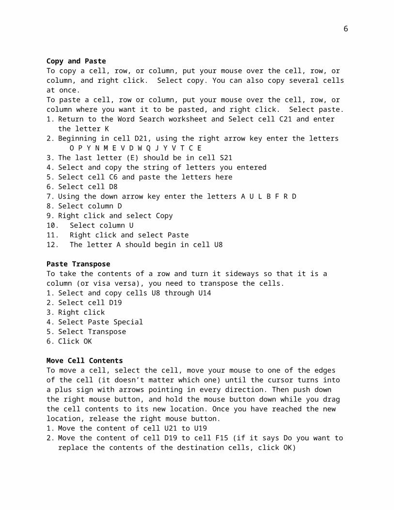
To copy a cell, row, or column, put your mouse over the cell, row, or column, and right click. Select copy. You can also copy several cells at once.To paste a cell, row or column, put your mouse over the cell, row, or column where you want it to be pasted, and right click. Select paste.1. Return to the Word Search worksheet and Select cell C21 and enter the letter K2. Beginning in cell D21, using the right arrow key enter the letters

O P Y N M E V D W Q J Y V T C E 3. The last letter (E) should be in cell S214. Select and copy the string of letters you entered 5. Select cell C6 and paste the letters here 6. Select cell D87. Using the down arrow key enter the letters A U L B F R D8. Select column D9. Right click and select Copy 10. Select column U11. Right click and select Paste12. The letter A should begin in cell U8

Paste TransposeTo take the contents of a row and turn it sideways so that it is a column (or visa versa), you need to transpose the cells.1. Select and copy cells U8 through U142. Select cell D193. Right click4. Select Paste Special5. Select Transpose6. Click OK

Move Cell ContentsTo move a cell, select the cell, move your mouse to one of the edges of the cell (it doesn’t matter which one) until the cursor turns into a plus sign with arrows pointing in every direction. Then push down the right mouse button, and hold the mouse button down while you drag the cell contents to its new location. Once you have reached the new location, release the right mouse button.1. Move the content of cell U21 to U192. Move the content of cell D19 to cell F15 (if it says Do you want to replace the contents of the

destination cells, click OK)

Fill Down1. Select cell B5 2. Using the down arrow key enter the letters Q C X S W P L M Y X I 3. Select cells B5 through B154. Move the cursor to the bottom right corner of cell B15 until the black cross appears (not the one with

the arrows pointing in every direction)5. Hold down the left mouse button, while dragging the mouse down6. Keep dragging until the mouse is over cell B22 then release the mouse 7. When the Auto-fill options box appears below the table drag the mouse over the box and click on the

downward arrow when it appears8. Select Fill Without Formatting to fix the table border9. Select cell V5 10. Using the down arrow key enter the letters H F T S Q I M Y W Z A11. Select cells V5 through V15

6

12. Use Fill Down to fill in the numbers up to cell V2213. When the Auto-fill options box appears below the table click the down arrow14. Select Fill Without Formatting15. Fill in the remaining cells with any capitalized letters16. Use Fill Down or copy cells to make this process easier17. Leave a blank cell between the words EMOTIONAL and AWARENESS

Creating a Word List1. Select column Y2. Go to the Home tab.3. In the Cells section, click Format4. From the drop down menu select Column Width5. Enter 19 in the Column width box 6. Click OK7. Enter “Word List” in cell Y58. Highlight the title Word List 9. Right click and select Format Cells10. Under Font scroll down and select Bookman Old Style11. Under Font Style select Bold12. Under Underline select Single 13. Under Color select Sea Green14. Click OK15. Enter the term Psychology in cell Y616. In cells Y6-Y15 enter the remaining terms and names: Skinner, Bandura, Freud, Emotional

Awareness, ANOVA, Control, Dendrites, Data and PSICHI17. Select column Y18. Right click and select Format Cells 19. Select the Alignment tab20. Under Horizontal select Center21. Click OK

Creating GroupsCreating groups in excel allows you to condense a section. This can be useful when you are using a large excel file with many tasks and project since it allows you to condense tasks you have completed or check on tasks for that specific project.1.In your word list, highlight rows Y6-Y15.2. Go to the Data tab, click Group3. You have now group all the words under “Word List”. This is indicated by the line on the left hand side of the screen. There will be a little (+) or (-) which you can click to condense or expand this section. To ungroup the section, just highlight the section and click Ungroup in the Data tab.

Creating a Hyperlink to Another Tab Using the Hyperlink ButtonCreating a hyperlink in the excel file allows you to click a hyperlink on one sheet that will quickly take you to another sheet so you don’t have to search for the tab. This is especially useful when dealing with an excel file that contains many more sheets that you can easily see on the bottom of the page. For our exercise, you will want to link the sheet “Answer Key” in our “Word Search” sheet. The Hyperlink button works the same way for when you are creating a hyperlink to an internet address and to a sheet in another excel file.1.In the Word Search Tab, write the word Answer Key to the right of your word search. 2. Highlight the words Answer Key and Right Click it.3. From the drop down menu, click Hyperlink.

7

4. In the new box, under Link to, select Place in This Document5. To the right under “Or Select a place in this document”, select ‘Answer Key’ and press Ok.6. You have just created a hyperlink that will take you directly to the ‘Answer Key’ sheet from the ‘Word Search’ sheet. 7. You can follow the same process to link to a specific section in another sheet, workbook, or website as well. The only thing that changes in the process is what you select in the ‘Link to’ section.8. To undo your hyperlink, right click the hyperlink and click ‘Undo hypperlink’ from the drop down menu.

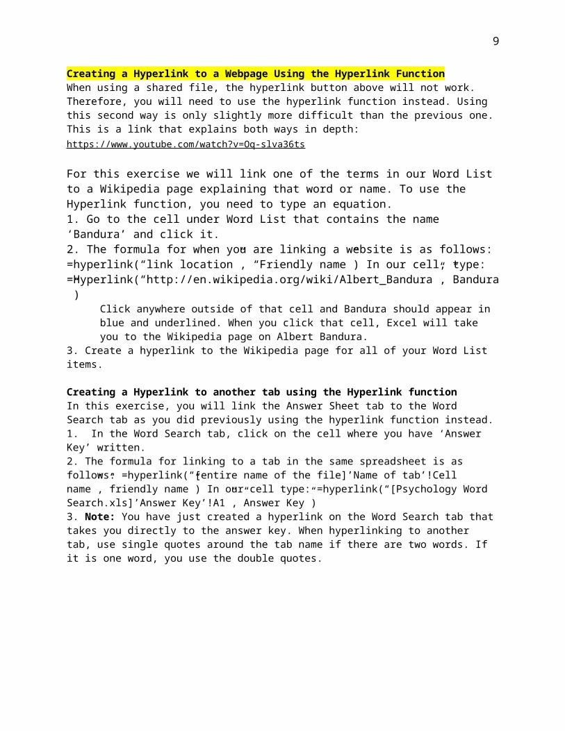
Creating a Hyperlink to a Webpage Using the Hyperlink FunctionWhen using a shared file, the hyperlink button above will not work. Therefore, you will need to use the hyperlink function instead. Using this second way is only slightly more difficult than the previous one. This is a link that explains both ways in depth: https://www.youtube.com/watch?v=Oq-slva36ts

For this exercise we will link one of the terms in our Word List to a Wikipedia page explaining that word or name. To use the Hyperlink function, you need to type an equation. 1. Go to the cell under Word List that contains the name ‘Bandura’ and click it.2. The formula for when you are linking a website is as follows: =hyperlink(“link location”, “Friendly name”) In our cell, type: =Hyperlink(“http://en.wikipedia.org/wiki/Albert_Bandura”,”Bandura”)

Click anywhere outside of that cell and Bandura should appear in blue and underlined. When you click that cell, Excel will take you to the Wikipedia page on Albert Bandura.

3. Create a hyperlink to the Wikipedia page for all of your Word List items.

Creating a Hyperlink to another tab using the Hyperlink functionIn this exercise, you will link the Answer Sheet tab to the Word Search tab as you did previously using the hyperlink function instead.1. In the Word Search tab, click on the cell where you have ‘Answer Key’ written.2. The formula for linking to a tab in the same spreadsheet is as follows: =hyperlink(“[entire name of the file]’Name of tab’!Cell name”,”friendly name”) In our cell type: =hyperlink(“[Psychology Word Search.xls]’Answer Key’!A1”,”Answer Key”)3. Note: You have just created a hyperlink on the Word Search tab that takes you directly to the answer key. When hyperlinking to another tab, use single quotes around the tab name if there are two words. If it is one word, you use the double quotes.

8

Lesson 2: Advanced Excel (Data Management)

PurposeIn this workshop, you will learn how to use different applications to manage data. These applications include learning the following: concatenate, variable labels, and paste special / values. To concatenate is to link items together in a chain or series. Excel can easily concatenate items to create lines of code by using simple equations.

PrerequisitesYou should have successfully completed Lesson 1: Introduction to Excel, before attempting this lesson.

Application 1: Variable LabelsThe POES calculates 4 types of scores for each of 20 items and a total score. The four types of scores are Highest-4 (H4), All-Sum (AS), 334 (34), and 3345 (35). For each item and scoring method, it generates scores for the three different parts of the item: Self, Other, and Total. You will use Excel to create variable labels for each of the 21 (20 item scores + 1 total score) * 4 (methods) * 3 (self, other total) = 252 variables. The labels should use the following format:

LEAS.SC.AS.Item.12.O The word “LEAS”, whether or not the data was spell-checked (“SC”), scoring method (“AS”), the word “Item”, item number (“12”), item part(“O”)

1. Open a new excel file2. In cell A1, type LEAS3. In cell B1, type a period4. Use Fill Down to copy A1 and B1 into the cells in rows 2 through 2525. In cell C1, type SC6. In cell D1, type a period7. Use Fill Down to copy C1 and D2 into the cells in rows 2 through 252.8. In column E, type the four types of scoring methods. In E1, type H4. In E2, type AS. In E3, type 34.

In E4, type 35.9. In cell E5, type the formula =E110. Use Fill Down, to copy the formula in E5 to the rest of the cells in column E.11. Left align column E12. In cell F1, type a period. Use Fill Down to copy this period into the rest of the cells in column F.13. In cell G1, type Item. In cell H1, type a period. Use Fill Down.14. In cells I1, I2, I3, and I4, type the number 1.15. In cell I5, type the formula =I1+116. Use Fill Down to copy the formula in I5 to the cells I6 through I84.17. In cell I85, type the formula =I118. Use Fill Down to copy the formula in I85 to the rest of the cells in column I.19. Select column I20. Right click, and select Copy21. Right click, and select Paste Special22. Select Values, and click OK23. In column I, where you see the number 21, type Tot. For example, you get some 21’s around row 81.

Some more around row 165. Some more around row 249.24. Left align column I.25. In cell J1, type a period. Use Fill Down to copy it to the rest of the cells in column J.26. In cell K1, type S27. Use Fill Down to copy this S to the cells up to row 84.28. In cell K85, type O29. Use Fill Down to copy this O to the cells up to row 168.

9

30. In cell K169, type T31. Use Fill Down to copy this T to the cells up to row 252.32. In cell L1, type the formula =concatenate(A1, B1, C1, D1, E1, F1, G1, H1, I1, J1,K1)33. Use Fill Down to copy this formula to the rest of the cells in column L34. Congratulations! You did it! If you were analyzing these variables in SPSS, you could copy these

labels directly into SPSS at this point.

10

Application 2: Getting ID’s to RepeatIn our LEAS data entry, the ID is given at the top of each participant. When we go to score this data with POES, we need to get the ID to show up as the first line before EVERY item, so that column A has an ID in every row.

1. Open Workshops on Excel Getting IDs to repeat example.xls (in the Lab Meetings folder on the cluster server).

2. Save the file to the desktop so that you do not destroy the example file.3. On the saved sample file, insert a new column before the first column. This new column will now be

called column A.4. For the first participant, in column A, type consecutive numbers in each row. We are numbering the

rows for the participant.5. For the remaining participants, we will use formulas to get these row numbers. In cell A5, type =a1.

Select cell A5. Use fill down to copy this formula to the rest of the cells in column A, to number the rows for all remaining participants.

6. Insert a new column before the first column. This new column will now be called Column A.7. In cell A1, type the formula =c1. This will put the first ID in the first cell in Column A.8. We want to put ID’s in every row in Column A. We will use an IF statement. In cell A2, type the

following =if(b2<b1,c2, a1)What this is saying is, if b2 < b1, then this is a new participant. In that case, we should use the ID that is found in column C. Otherwise, this row is the same participant as the previous row, and we should use the same ID as we used for the last row.

9. Select cell A2. Use Fill Down to copy this formula to the rest of the rows next to participant data.10. The ID’s we have right now are formulas. If we rearranged the data at all, the formulas would not do

what we want them to do. We need to change these formulas into numbers. Select Column A. Right click, Copy. Right click, Paste Special, Values, OK.

11. Check that column A has the right ID numbers. Compare them to the ID’s in Column C. When are you are sure that this worked properly, delete columns B and C.

12. Congratulations! You did it! Getting the ID’s to repeat in the first column of the Excel spreadsheet is one of the steps we have to do to get the LEAS data ready to be scored by POES. There are a few other steps. For example, we have to remove the commas. But this is one of the hardest and most important steps.

11

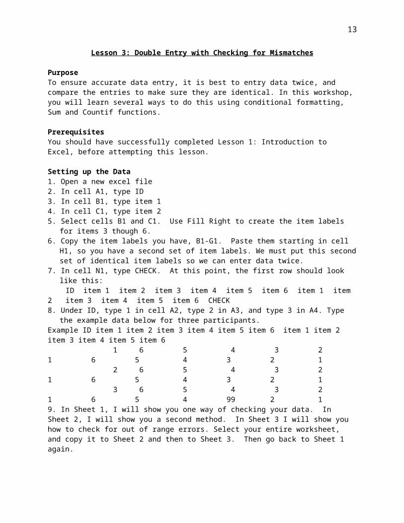
Lesson 3: Double Entry with Checking for Mismatches

PurposeTo ensure accurate data entry, it is best to entry data twice, and compare the entries to make sure they are identical. In this workshop, you will learn several ways to do this using conditional formatting, Sum and Countif functions.

PrerequisitesYou should have successfully completed Lesson 1: Introduction to Excel, before attempting this lesson.

Setting up the Data1. Open a new excel file2. In cell A1, type ID3. In cell B1, type item 14. In cell C1, type item 25. Select cells B1 and C1. Use Fill Right to create the item labels for items 3 though 6. 6. Copy the item labels you have, B1-G1. Paste them starting in cell H1, so you have a second set of item

labels. We must put this second set of identical item labels so we can enter data twice.7. In cell N1, type CHECK. At this point, the first row should look like this:

ID item 1 item 2 item 3 item 4 item 5 item 6 item 1 item 2item 3 item 4 item 5 item 6 CHECK

8. Under ID, type 1 in cell A2, type 2 in A3, and type 3 in A4. Type the example data below for three participants.

Example ID item 1 item 2 item 3 item 4 item 5 item 6 item 1 item 2 item 3 item 4 item 5 item 6 1 6 5 4 3 2 1 6 5 4 3 2 1 2 6 5 4 3 2 1 6 5 4 3 2 1 3 6 5 4 3 2 1 6 5 4 99 2 19. In Sheet 1, I will show you one way of checking your data. In Sheet 2, I will show you a second method. In Sheet 3 I will show you how to check for out of range errors. Select your entire worksheet, and copy it to Sheet 2 and then to Sheet 3. Then go back to Sheet 1 again.

12

Method 1The first method of checking for mismatches is to calculate the sum of the squared differences of the values.

Checking for Mistakes10. Go to Sheet 1 and copy the item labels for your six items (B1-G1), and paste them starting in cell O1,

so you have a third set of item labels.11. In cell O2, type =(B2-H2)^2 You can type the cell references to B2 and H2, or you can use the

mouse to select these cells. The ^ symbol is shift-6. This formula will calculate the difference between the numbers you typed for the first and second time you entered the data for the first participant. It will then square that difference. If the two numbers match, this should evaluate to 0 when you hit the enter key.

12. Use Fill Right to copy this formula to the rest of the cells O2 to T2 in row 2, so that you have formulas for all six items.

13. Select cells O2 through T2. Then use Fill Down to copy this formula to the two rows below, so that you have formulas for all three participants. You will notice that one of these cells is NOT 0. That’s because there is a mismatch. And Excel is now showing you where that mismatch is.

14. In cell N2, type =sum(O2:T2) You can type the cell references to O2 and T2, or you can use the mouse to select this range of cells

15. Use Fill Down to copy this formula to the rest of the participants. You can see that one subject where cell N4 there is a mismatch. It doesn’t evaluate to 0.

Highlighting16. Select columns N through T17. Under the Home tab, in the Styles section, click Conditional Formatting.18. From the dropdown menu, go to Highlight Cells Rule/Greater than19. Type 0 and choose Red Text.20. Click OK. Look how the non-zero numbers are highlighted.**21. Select row 122. Click on Format, Conditional Formatting.23. Click Delete. Select condition 1. Click on Clear Rules. Then click on Clear Rules from Selected Cells.

Click OK. Click OK. This just makes it look nicer. 24. Congratulations! You have now created a worksheet that checks for mismatches, and which highlights both the subject and the individual response that don’t match. This is the method that I personally use when I am entering grades, because it is so easy to set up.

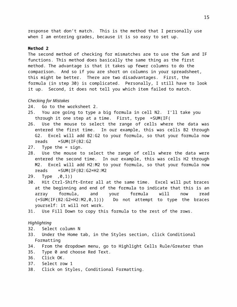
Method 2The second method of checking for mismatches are to use the Sum and IF functions. This method does basically the same thing as the first method. The advantage is that it takes up fewer columns to do the comparison. And so if you are short on columns in your spreadsheet, this might be better. There are two disadvantages. First, the formula (in step 30) is complicated. Personally, I still have to look it up. Second, it does not tell you which item failed to match.

Checking for Mistakes24. Go to the worksheet 2.25. You are going to type a big formula in cell N2. I’ll take you through it one step at a time. First, type

=SUM(IF(26. Use the mouse to select the range of cells where the data was entered the first time. In our example,

this was cells B2 through G2. Excel will add B2:G2 to your formula, so that your formula now reads =SUM(IF(B2:G2

27. Type the = sign.

13

28. Use the mouse to select the range of cells where the data were entered the second time. In our example, this was cells H2 through M2. Excel will add H2:M2 to your formula, so that your formula now reads =SUM(IF(B2:G2=H2:M2

29. Type ,0,1))30. Hit Ctrl-Shift-Enter all at the same time. Excel will put braces at the beginning and end of the

formula to indicate that this is an array formula, and your formula will now read {=SUM(IF(B2:G2=H2:M2,0,1))} Do not attempt to type the braces yourself: it will not work.

31. Use Fill Down to copy this formula to the rest of the rows.

Highlighting32. Select column N33. Under the Home tab, in the Styles section, click Conditional Formatting34. From the dropdown menu, go to Highlight Cells Rule/Greater than35. Type 0 and choose Red Text.36. Click OK.37. Select row 138. Click on Styles, Conditional Formatting.39. Click Delete. Click Clear Rules. Click Clear Rules from Selected Cells. Select condition 1. Click

OK. Click OK.

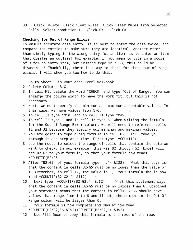
Checking for Out of Range ErrorsTo ensure accurate data entry, it is best to enter the data twice, and compare the entries to make sure they are identical. Another error than simply typing in the wrong entry for an item, is to enter an item that creates an outlier! For example, if you mean to type in a score of 3 for an entry item, but instead type in a 33, this could be disastrous! Thankfully, there is a way to check for these out of range errors. I will show you two how to do this.

1. Go to Sheet 3 in your open Excel Workbook.2. Delete Columns B-G.3. In cell H1, delete the word “CHECK” and type “Out of Range.” You can enlarge the column width to

have the work fit, but this is not necessary. 4. Next, we must specify the minimum and maximum acceptable values. In this case, we have values

from 1-6.5. In cell I1 type “Min” and in cell J1 type “Max.”6. In cell I2 type 1 and in cell J2 type 6. When writing the formula for the Out of Range Error column,

we will need to reference cells I2 and J2 because they specify our minimum and maximum values. 7. You are going to type a big formula in cell H2. I’ll take you through it one step at a time. First type

=COUNTIF(8. Use the mouse to select the range of cells that contain the data we want to check. In our example, this

was B2 through G2. Excel will add B2:G2 to your formula, so that your formula now reads =COUNTIF(B2:G5

9. After “B2:G5” of your formula type ,“<”&I$2) What this says is that the content in cells B2-G5 must be no lower than the value of 1. (Remember, in cell I2, the value is 1). Your formula should now read =COUNTIF(B2:G2,“<”&I$2)

10. Next type +COUNTIF(B2:G2,“>”&J$2) What this statement says that the content in cells B2-G5 must be no larger than 6. Combined, your statement means that the content in cells B2-G5 should have values that range from 1 to 6 and if not, the number in the Out Of Range column will be larger than 0.

11. Your formula is now complete and should now read =COUNTIF(B2:G2,“<”&I$2)+COUNTIF(B2:G2,“>”&J$2)

12. Use Fill Down to copy this formula to the rest of the rows.

14

13. Cells H2 and H3 should have Zeros. Cell H4 should have a 1. This means that there is one cell in the cell range that is not an acceptable value and is outside our minimum and maximum value range.

Cell ProtectionNow that you typed all those long and complicated formulas, you don’t want anyone to mess them up! This is quite easily done through the “copy and paste” function, adding additional rows, or even simply if someone accidentally over-types those cells so the easiest way to avoid this is to prevent it! I will show you how to protect your cells and the formulas in them.

1. Select column H.2. Right click and go to the Format Cells Menu.3. Under the Protection Tab, make sure the box next to “Locked” is checked. Then click OKAY. This

will lock all the cells in column H. This means that now no one can type, click, or do any formatting in those cells

4. Now select columns A-G. 5. Right click and go to the Format Cells menu.6. Under the Protection Tab, make sure the box next to “Locked” is NOT checked. These are the

columns that we will allow people to type in. These columns contain no formulas.7. Under the Review tab, in the Changes section, click Protect Sheet. Under the Home tab, in the cells

section, click Format and then select “Protect Sheet.” You may enter a password. This will prevent anyone without the password from unlocking the locked cells.

8. Congratulations! Your formulas are safe!9. To prepare for the next lesson, unprotect your sheet and do not exit out of the workbook.

15

Lesson 4: Advanced Skills for Data Entry (file sharing and split window)

PurposeIn the previous lesson, you learned the basics of doing double data-entry. In this lesson, you will master more advanced topics of data entry, including a safe way to work on data entry simultaneously, as well as freezing columns and rows.

Prerequisites You should have successfully completed Lesson 1: Introduction to Excel and Lesson 3: Double Entry with Checking for Mismatches before attempting this lesson.

Part 1: File-Sharing

PurposeIn order to facilitate and quicken data entry, it is possible to have more then one person work on entering data at one time. There are two options to enter data simultaneously.

The first option is to have each person enter data on separate Excel files. However, there are disadvantages to this method. One person entering data entry cannot see what has been entered by others, so some data could be entered twice or more. Along the same lines, one person doing data entry could assume that another person has already entered some specific set of data, which means that there is a risk of some data not being entered.

Instead, it is possible to enable an Excel file to be worked on simultaneously. This allows the people doing the data entry to see what has been entered already. However, specific steps must be taken in order to ensure that no data is lost.

Setting Up Spreadsheet For File-Sharing1. Open the file from Lesson 3. It does not matter whether you use Sheet 1 or Sheet 2 for this lesson. It

is highly advised to have all the components of the file ready for data-entry before enabling file-sharing.

2. Under the Review tab, select Share Workbook.3. Under the Editing tab, select “Allow changes by more than one user at the same time” and click OK.4. The file can now be shared.

IMPORTANT: If you are working on data entry while you are in the lab and wish to save your progress, check if anyone else is working on the same file. If there is no one working on the file, proceed with the save. However, if there is a person(s) working on the file, ask them to stop what they are doing while you proceed with the save. After the file is saved, inform the others that they can continue with the data entry. This is very important, as if they do not stop entering data as you save, it is possible that data will be lost.

16

Part 2: Split Window

PurposeNow that we have learned to allow people to work on the file simultaneously, we can now move on to making data entry easier.

Most of the time, there are so many participants and/or items, that the headings of the rows and columns will be lost if you scroll elsewhere in the sheet.

This can be easily remedied by splitting the window, which allows chosen rows and/or columns to be visible at all times.

Splitting the Window 1. Open the Excel file from Lesson 3, and select Sheet 1.2. Select the cell immediately below the column headings and immediately to the right of the row

headings. This will be B2 in this file.3. Under the View tab, in the Windows section, click split.4. To remove the split, click on split again.5. Scroll through the file to ensure that row 1 and column A are always visible.

17

Lesson 5: Creating Frequency Tables Using Pivot Tables

PurposeIn this lesson you will be learning how to use array formulae, histograms, and pivot tables / chart wizard. You will begin be watching two videos. The first is on frequency distributions and the second is on hands-on frequency distributions.

PrerequisitesYou should have successfully completed Lesson 1: Introduction to Excel, before attempting this lesson.

Part I: Video on Frequency Distributions

Watch the video located at http://twopaces.com/stats_help.html#videos entitled “Simple Frequency Distribution in Excel”.

Part II: Hands-on Frequency Distributions

Getting Ready1. First watch the video, in Part I.2. Open Excel 2007.3. Click the Microsoft Office Button, and then click Excel Options.4. Click Add-Ins, and then in the Manage box, select Excel Add-ins. Click Go. 5. In the Add-Ins available box, select the Analysis ToolPak check box, and then click OK. If Analysis

ToolPak is not listed in the Add-Ins available box, click Browse to locate it. If you get prompted that the Analysis ToolPak is not currently installed on your computer, click Yes to install it.

6. After you load the Analysis ToolPak, the Data Analysis command is available in the Analysis group on the Data tab.

Opening Example Data1. Open the Example file, Intermediate Excel 1, which is designed to go with this lesson. Open the

cluster server, open Barchards Lab, open Lab Meetings and Training, and open Workshops on Excel Frequency Tables Example Data.xls

2. Select entire file and copy. Open a new file and paste.

Array Formula1. Rearrange the possible values of X in descending order from 10-1. Select cells B2-B11. Under the

Home tab, in the Editing section, click on Sort and Filter. Select Sort Largest to Smallest. A message box will pop out. Select continue with the current selection.

2. Select cells C2-C11.3. Enter =FREQUENCY(A2:A31, B2:B11) in the formula bar. Then hold down the control and shift

buttons while at the same time pressing enter. Your formula should now look like: =FREQUENCY(A2:A31, B2:B11)}. This counts the frequency within this data range for all the possible values of X at once.

Histogram

18

1. Sort X values in ascending order. (Do this the same way you sorted them in descending order except choose Sort Smallest to Largest.) A message box will pop out. Select continue with the current selection. F(x) values will automatically rearrange themselves.

2. Click on the Data tab.3. Under the Analysis section, click Data Analysis. 4. Select Histogram.5. For Input Range select the data (A2 – A31). It should look like this: $A$2:$A$316. For the Bin Range select B2-B11. It should look like this: $B$2:$B$117. Select Output Range which will be put under column D. It should look like this: $D$18. Click OK.

Pivot Table or Pivot Chart Wizard1. Go to the Insert tab.2. Under the Tables section, click Pivot Table. Choose Pivot table from the drop down menu.3. A message box will come up and ask “where is the data you want to use?” Select cells A1-A31. It

should look like this: Data!$A$1:$A$314. Where it says, “where do you want to put the Pivot Table report?” Select Existing worksheet. 5. Click on Select cell F1. This should look like this: Data!$F$1 under existing worksheet.6. Click OK.7. In the Pivot Table Field List, drag grades from the menu that appears to the right to the “drop row

fields here”.8. In the Pivot Table Field List, drag grades to the “drop data items here”.9. Select cell F1 and right click.10. Select value field settings.11. Select Count. Next to name it should now read: Count of grades.12. Click ok.

19

Lesson 6: Look-up Tables

PurposeLookup tables are a very effective tool that is in Microsoft Excel. If you are using multiple sheets and want values from one sheet in another sheet, you can use the lookup tool so that it will fill in the information without having to bounce back and forth looking at the values yourself. This workshop shows you how to use lookup tables to generate random passwords for participants. The purpose is that it takes the letters you have typed in another sheet and inputs them into your first sheet without you having to bounce back and forth.

Prerequisites You should have successfully completed Lesson 1: Introduction to Excel and Lesson 2: Advanced Excel (Data Management).

Making a Look-up Table in Excel1. Open Microsoft Excel2. Right click on the tab marked Sheet 1 at the bottom of the screen. Click on Rename. rename it to

“Consonant Lookup”. Rename the other two tabs making the tab Sheet 2 “Vowel Lookup”, and Sheet 3 “Password”.

3. On the consonants lookup sheet (the first sheet), type in the consonants of the alphabet in the first column (A) starting with the letter b in cell A1. Omit the letters x and q however, because they are confusing to remember in a password. So the column should end with the letter z in cell A19

4. In column B, type in the numbers 1 through 19. The cell B1 should have the number 1 and the cell B19 should have the number 19

5. On the vowel lookup sheet (the second sheet), type in the vowels of the alphabet in column A staring with a in cell A1 and ending with u in cell in A5

6. In column B, type in the numbers 1 through 5. The cell B1 should have the number 1 and the cell B5 should have the number 5.

7. In the Password sheet, we are first going to give names to the columns to make it easier later on to remember what they stand for. In row 1 type the following in the cells:

a. A1- “Consonant”, B1- “Vowel”, C1- “Consonant”, D1 leave empty, E1-“Consonant”, F1- “Vowel”, G1- “Consonant”

b. Now skip over to cell L1 and type the word “Password” and in cell N1 type the word “Password”

8. In row 2, type in the word “rnd num” in cells A2, B2, C2, H2, I2, and J2. 9. In cell L2 type “changeable” and in cell N2 type “(use paste special/value/ to fix the values)” this

will help you remember later how to keep previous passwords.a. The first three columns pick a random number value. The next three columns take that

number and “look up” the consonant or vowel that was assigned that number in the lookup sheets. The rnd num sheets again choose a random number to accompany the letters and the password columns show the resulting password. We use two password columns because sometimes the passwords have a combination of letters of numbers that is confusing so we would like to change just that one password. When you change that one however, the sheet automatically produces new passwords for all of them. This is why we paste all the resulting passwords into the column N so that we can keep passwords that we like written down.

10. Now we will make the functions to produce our desired numbers and letters. First column labeled Consonant

a. Type “=TRUNC(RAND()*19+1,0)” into the fx tool bar into cell A3.b. Click on the cell then click and hold on the black box in the lower right hand corner of the

cell. To fill in the first 20 cells (e.g. A3-A20) in the column with the random numbers drag the curser down filling in the cells.

20

Second column labeled vowel. a. Type “=TRUNC(RAND()*5+1,0)” in the fx tool bar. b. Use the fill down again to fill the first twenty cells (e.g. B3-B20) for the vowels

Third column labeled consonant.a. Repeat the same steps as the first column labeled consonant.

11. Click on cell E3, then go to the Formulas Tab, Click on Lookup & Reference, then LOOKUP. 12. A box will pop up and ask if you want lookup values with a lookup vector and result vector or just a

lookup with an array, you want the option of the lookup vector with the result vector. Once this is highlighted, click ok. Type the following in the boxes

a. Lookup_value A3b. Lookup_vector ‘Consonant lookup’!$B$1:$B$19c. Result_vector ‘Consonant lookup’!$A$1:$A$19

Makes sure these are typed exactly then click ok. The functions should produce a letter and the fx box should say, “= LOOKUP(A3,'consonants lookup'!$B$1:$B$19,'consonants lookup'!$A$1:$A$19)”. Go ahead and fill down for the first 20 boxes.

13. Click on the cell F3 then go to the Formulas Tab, Click on Lookup & Reference, LOOKUP and repeat the steps above, except the boxes should now say:

a. Lookup_value B3b. Lookup_vector ‘vowel lookup’!$B$1:$B$5c. Result_vector ‘vowel lookup’!$A$1:$A$5

Again, make sure these are typed exactly right then click ok. The function should produce a vowel and the fx box should say, “=LOOKUP(B3,'vowel lookup'!$B$1:$B$5,'vowel lookup'!$A$1:$A$5)”. Go ahead and fill down for the first 20 boxes.

14. For the cell G3 repeat the steps in 12. with the lookup_value of C3. The resulting function should look like “= LOOKUP(C3,'consonants lookup'!$B$1:$B$19,'consonants lookup'!$A$1:$A$19)”

15. For the columns H I J, we are again going to use the Trunc function. Click on cell H3 then type “=TRUNC(RAND()*10,0)” into the fx bar.

a. Go ahead and fill down for the first 20 boxes. b. Then using the same method drag the curser to the right to fill in columns I and J.

16. YAY! You know have all the pieces for your password, Let’s put them together now!17. Type “=CONCATENATE(E3,F3,G3,H3,I3,J3)” into the fx bar in cell L3. Use the fill down function

for the first twenty cells (e.g. L3-L20). 18. Now as you have seen throughout the workshop, the cells do change the numbers and letters every

time you change something in the spreadsheet. Now we want to save the passwords we like. Highlight the cells in column L from cells L3 down to L20, on the toolbar, click on the Home Tab then click on copy, go over and click on cell N3,then go back up to the paste drop down menu, click on paste special, make sure the button for values is checked and in operation that is says none, everything else should be left blank. Then click ok.

19. You have successfully used the lookup tables application! Enjoy!

21

Lesson 7: Using Excel to Calculate Statistics

PurposeExcel can be used to calculate a variety of statistics. This workshop will teach you how to calculate central tendency, correlations, and the sums of squares that are used to calculate the variance and standard deviation and which are also used to calculate ANOVAs.

Prerequisites You should have success completed lesson 1: Introduction to Excel.

Assignment1. Open the file Using Excel to Calculate Statistics by Frank LoSchiavo June 2009.xls2. .Save the file to the desktop.3. Using the instructions given in the spreadsheet, calculated the indicated statistics, confirming that

each calculation is done correctly.4. Delete the file you put on the desktop.

22

Lesson 8: How to create simple macros in Excel

PurposeThe purpose of this workshop is to write a simple macro. Macros are shortcuts to repeat task in excel. This can be very helpful in the lab as well as personal projects in life.

PrerequisitesYou should have successfully completed Lesson 1: Introduction to Excel, before attempting this lesson.

ComputerYou can do this lesson using almost any computer that has Excel 2007. However, there are two computers in the lab that you MAY NOT USE for this lesson. These are the two computers that we use to run the Data Checking Study. Those two computers have macros on them that are essential for running the Data Checking Study, and we don’t want to risk messing them up. You can use the computers that are in the main room or the front office.

Part 1: Creating a Macro

Recording Your MacrosHere you will create a task and the shortcut for excel to complete it. 1. Open Microsoft Excel to open a new workbook.2. Click the start button at the top right of Excel and Save the workbook as “My list of psychology

courses.”3. After you’ve saved your workbook, click on the “View” tab at the top of the workbook. 4. There will be a new menu at the top of your screen. Click the “Macros” button. (This button is the

last button on the top of your screen).5. After you’ve clicked on the “Macros” button, there are going to be three options, “View Macros,”

“Record Macros,” and “Use Relative References.” Click the “Record Macros option.”6. Another menu will appear that says “Record Macros.” In the “Macro Name” section, type

“Psychologycourses.” (Be sure NOT to include a space in the name).7. In the “Shortcut Key” section, type the letter you want to use for your macro. (To make this easy,

we will use the lowercase letter “p”).8. In the “Store Macro in” drop down menu, select “Personal Macro Workbook.”9. In the “Description” section, you can type a brief description of your macro. This will be more

useful when you start to write more complicated Macros. 10. Click ok to start recording your macro.11. In cell A1 “Psychology Courses.”12. In cells A2 and A3 type “Psy 210” in A2 and “Psy 240” in A3 and press enter.13. In cells A4 and A5 type “Psy 403” in A4 and “Psy 405” in A5 and press enter.14. In cells A6 and A7 type “Psy 441” In A6 and “Psy 460” in A7 and press enter.15. After you have typed all of this in, in the lower left corner there will be a little blue rectangle.

Click the blue rectangle to stop recording your macro.Congratulations you have just recorded your first macro!

Checking your workYou will be checking to see if your macro works. 1. To check to see if your macros works, click the start button at the top left corner of the excel file

to open a new spreadsheet. 2. Once you open a new sheet, press Ctrl p.3. After you have presses Crtl p, your list should appear in the exact cells that you typed all your

information in.