LES-tree: A Spatio-temporal Access Method based on ... · [email protected] Gonzalo Navarro...

LES-tree: A Spatio-temporal Access Method based on Snapshots

and Events ∗

Gilberto A. GutierrezCenter for Web ResearchUniversity of Chile andUniversity of Bıo-Bıo

Avenida La Castilla S/NChillan / Chile

[email protected]

Gonzalo NavarroCenter for Web Research and

Department of Computer ScienceUniversity of Chile.

Avenida Blanco encalada 2120Santiago / Chile

[email protected]

M. Andrea RodrıguezDepartment of Computer Science

University of ConcepcionEdmundo LarenasConcepcion / [email protected]

October 14, 2008

Abstract

This work presents a new access method (LES-tree)for spatio-temporal databases that handles discretechange events over objects’ spatial attributes. Themain characteristic of this structure is that, inaddition to the traditional database snapshots, LES-tree explicitly stores the events in log structuresassociated with space partitions. The definition ofthis new access method aims to extend capabilities ofcurrent spatio-temporal access methods to queries onevents, while competing with current structures fortraditional time-slice and time-interval queries. Thepaper describes the structure and presents favorableexperimental cost analyses of the structure.

∗This work was partially funded by Millennium NucleusCenter for Web Research, grant P04-067-F, Mideplan, Chile.Gilberto Gutierrez was also funded by research grant 0732184/R, University of Bıo-Bıo, Chile

1 Introduction

Spatio-temporal databases are composed of spatialobjects that change their location or shape atdifferent time instants [18]. Their objective is tomodel and represent the dynamic nature of real-worldapplications [10]. Examples of these applicationsare transportation, monitoring, environmental, andmultimedia systems. Spatio-temporal applicationshave been classified into three categories dependingon the type of data they manage [12]:

a) Applications that deal with continuous changes,such as the movement of a car on a highway.

b) Applications that involve objects that changetheir location in space by modifying their shapeor by a movement in a discrete manner. Anexample is the change in the administrativeboundary of a city over time.

1

c) Applications that integrate both previousbehaviors. This type of applications appears inthe environmental area where it is necessary tomodel objects’ movement and objects’ geometricchanges over time.

Extending window/range queries in spatialdatabases, the most studied types of queries inspatio-temporal databases are time-slice and time-interval queries [16]. Time-slice queries retrieveall objects that intersect the query window ata particular time instant. Time-interval queriesextend the idea of time-slice queries by consideringconsecutive time instants. These queries focus onthe coordinate- or snapshot-based representationsof objects’ movement. In addition to this type ofrepresentation, recent studies have emphasized therelevance of handling events, encouraging researchin the integration of coordinate- and event-basedrepresentation [23, 3, 2]. Event representationenables to manage relationships between events,querying about objects’ states, and querying whenand why changes on objects occur.

There exist various spatio-temporal access meth-ods that are adequate for applications that handlediscrete changes of spatial objects. Some are RT-tree [24], HR-tree (Historical R-tree) [10, 11], 3D R-tree [21], HR+-tree [14], MV3R-tree [15] and OLQ(Overlapping Linear Quadtree) [22], among others.These structures are designed to answer time-sliceand time-interval queries about the history of thespatial attributes of objects. In addition, several ofthese existing spatio-temporal access methods alsohandle spatial changes of objects [10, 15, 21], butthey use data about these changes with the purposeof updating the underlying data structure. They donot keep data about changes as records of eventsoccurred over objects and, therefore, they cannotefficiently answer queries about events occurred ina time interval.

This work aims to define a new access methodthat can efficiently answer time-slice queries, time-interval queries, and queries on events. To the bestof our knowledge, only the preliminary work in [5]indexes events to process traditional time-slice andtime-interval queries. In this work, we also address

event-based queries that retrieve objects satisfyingan event predicate within a spatio-temporal window.For example, retrieve all objects that entered orcrossed a given spatial window within a time interval.These queries are easily extended to spatio-temporalpattern queries [7], where we may want to retrieveobjects that follow certain patterns of events in aparticular sequence.

Our new access method, LES-tree, is based onproducing snapshots after a certain number ofchanges occurred over objects, and on storing theevents that produce these changes in a data structurecalled a log. Consequently, LES-tree enables therepresentation of (1) temporal snapshots and (2)events on objects, as advocated in [23]. This approachhas been briefly discussed in others studies [8, 9],but it has been discarded a priori by arguing thatit is not easy to know how many events determinea new snapshot and that extra time is requiredfor query processing. We show in this paper thatthis is not a serious drawback. The number ofsnapshots represents a trade-off between space andanswer time, since a larger number of snapshotsdecreases the answer time of a query while increasingthe storage space. Inversely, a smaller number ofsnapshots decreases the space while increasing theanswer time; and then, the frequency of snapshotscan be adjusted depending on the type of applicationsand the change frequency of objects. For example,there may be applications where it is not of interestto query about objects’ states over some period oftime. Our data structures for snapshots and changesare independent, and so are the improvements thatcan be obtained in either structure. Furthermore,integration of existing spatial access methods forhandling snapshots into this approach can be easilyachieved.

The idea of snapshots and logs has also been usedwith the purpose of maintaining materialized viewsin a database [4]. In this context, a log is createdover the master table, from which the initial viewis created. Then, the refreshed view is the result ofapplying the changes stored in the log. These logs areeliminated after the actualization of the view, sinceonly the last state of the database is requested. Thelogs in our proposal, in contrast, are a part of the

2

indexing structure, remain over time, and can derivedifferent temporal states of the database.

A preliminary proposal of an access method withthese characteristics is the SEST-Index [5]. Theidea of SEST-Index consists in maintaining thesnapshots of the database for certain time instants(by using an R-tree) and having a global log to storethe events occurred between consecutive snapshots.The log is stored in time-order and allows us toreconstruct whatever the state of the database wasbetween two consecutive snapshots. Although thisstructure presents some good properties for time-sliceand event queries, it has serious storage cost andscalability problems, and its performance decreasesdrastically as the number of events increases.

This paper extends and complements substantiallythe proposal described in [5]. Instead of takingsnapshots at the (global) database granularity, itconsiders snapshots at the region granularity (leafsnapshots). These regions correspond to thespace partitions derived from the R-tree structureassociated with a global snapshot. The maincontributions of this work are:

i) It presents a new spatio-temporal access methodbased on snapshots and events. This newaccess method considers snapshots with regiongranularity. These regions are modified by theuse of global snapshots along time.

ii) It presents algorithms not only for time-slice,time-interval, but also for event queries.

iii) It experimentally compares the proposed datastructure against MVR-tree [15, 16], MV3R-tree[15], and the preliminary proposal SEST-Indexpublished in [5] for the different times of queries.To the best of our knowledge, MVR-tree andits improved varient MV3R-tree are structuresthat outperform previous spatio-temporal accessmethods in terms of time and space requirementsfor time-slice and time-interval queries. Resultsindicate that our spatio-temporal access methodhas better performance than SEST-Index andcompetes closely, or even overcomes, MVR-tree,including its improved variant .

The organization of the paper is as follows. Section2 reviews current spatio-temporal access methods forapplications that handle discrete changes. Section 3describes the proposed access method in terms of itsdata structure and operations. Section 4 describesand evaluates a cost model for LES-tree. Section 5gives experimental evaluations with respect to SEST-Index and MVR-tree. Conclusions and future workare given in Section 6.

2 Spatio-temporal access meth-

ods

This section describes the main spatio-temporalaccess methods available for applications of category(b) (see Section 1) that have been designed toanswer time-slice and time-interval queries. Wefocus on the MVR-tree/MV3R-tree and SEST-Indexstructures, against which we compare the newproposed structure. A classification of the existingspatio-temporal access methods is the following: (a)Methods that treat time as another dimension. (b)Methods that incorporate the temporal informationin the nodes of the structure without consideringtime as another dimension. (c) Methods basedon overlapping structures. (d) Methods based onmultiversioning of the structure. (e) Methods basedon snapshots and events.

The 3D R-tree [21] considers time as another axisalong with the spatial coordinates. In a three-dimensional space, two line segments ((xi, yi, ti),, (xi, yi, tj)) and ((xj , yj , tj), (xj , yj , tk)) model anobject that initially remains at (xi, yi) during thetime interval [ti, tj), and then it locates at (xj , yj)during the time interval [tj , tk). Such line segmentscan be indexed by a 3D R-tree. This idea works wellif all the final limits of the time intervals are knownin advance. The 3D R-tree structure is efficient inspace and in processing time-interval queries. It is,however, inefficient for processing time-slice queries[16].

RT-tree [24] is a structure where the temporalinformation is kept in the nodes of the R-tree.This is an extension to the data content of a

3

traditional R-tree. In this type of structure, thetemporal information plays a secondary role becausethe search is guided by the spatial information. Thus,queries with temporal conditions cannot be efficientlyprocessed [10].

HR-tree [11, 10] and MR-tree [24] are based onthe concept of overlapping. The basic idea is that,given two trees, the most recent tree corresponds toan evolution of the older tree, and subtrees can beshared between both trees. The major advantage ofthe HR-tree is its efficiency in processing time-slicequeries. Its major disadvantage is the excessive spacethat it requires to store the structure. For example,if only one object of each leaf node moves at instantti, the tree is completely duplicated at instant ti+1.

MVR-tree [15, 14, 16] is a structure based onhandling multiple versions. It is an extension ofMVB-tree [1], where the time-varying attribute isspatial. Similar to the MVB-tree, each entry in theMVR-tree is of the form 〈S, ts, te, pointer〉, whereS corresponds to a MBR. An entry is alive attime instant t if ts ≤ t < te and dead otherwise.MVR-tree imposes constraints on the number ofentries stored in its nodes. A constraint ensuresthat there exist either zero or at least b · pversion

alive entries in any non-leaf node at a time instantt, where pversion is a parameter of the tree and b

is the capacity of a node. This condition groupsalive entries at time instants for processing time-slice queries. Other constraints (namely, strongversion overflow and strong version underflow) ensurea good space usage in the algorithms for insertion anddeletion [15, 14, 16]. Like the MVB-tree, an MVR-tree has multiple R-trees (logical trees) that organizethe spatial information for non-overlapping temporalwindows. This structure outperforms the HR-tree inspace and time when processing short time-intervalqueries. A modification of MVR-tree called MV3R-tree [15] improves the performance of MVR-tree forlong time-interval queries by adding an auxiliary 3DR-tree for processing these queries. With the purposeof maintaining the storage within reasonable limits,both indices must share the same leaf pages, whichmakes the insertion algorithm rather complex.

A disadvantage of the MVR-tree is the insertionof artificial entries at the leaf nodes as it does not

guarantee that the real lifespan of an object is storedin only one node. For example, if an object O1

was at position S1 in a time interval [1, 20), theinsertion algorithm of MVR-tree may create twoentries 〈S1, 1, 8〉 and 〈S1, 8, 20〉 in two different nodes,making it more difficult to obtain the exact instantwhen the object O1 arrives or leaves the position S1.

SEST-Index [5] is a structure that maintainssnapshots for some time instants and stores theevents that occur between consecutive snapshots.One of the main disadvantages of SEST-Index is therapid growth of its size (storage use) as the numberof changes increases. This disadvantage is explainedbecause each snapshot duplicates all the objects,including those that have undergone no modificationbetween consecutive snapshots. A solution to thisproblem was proposed in [5], but it has two importantlimitations: (i) the objects must be points and (ii)the region where the changes occur must be fixed.The proposal in this paper follows some of the ideasof SEST-Index, but it overcomes the two previouslimitations and achieves good space usage, withoutcompromising time efficiency.

3 LES-tree: A Spatio-temporal

Access Method Based on

Snapshots and Events

Similar to SEST-Index [5], LES-tree maintainssnapshots for some time instants and stores theevents that occur between consecutive snapshots.One of the main disadvantages of SEST-Index isthe rapid growth of its size (storage use) as thenumber of changes increases. This disadvantageis explained because each snapshot duplicates allthe objects, including those that have undergoneno modification between consecutive snapshots. Asolution to this problem was proposed in [5], butit has two important limitations: (i) the objectsmust be points and (ii) the region where the changesoccur must be fixed. LES-tree overcomes these twolimitations and achieves good space usage, withoutcompromising time efficiency.

LES-tree considers two types of snapshots, which

4

handle different space granularity. The first typeof snapshots (global snapshot) corresponds to an R-tree (spatial indexing structure) including all objectsexisting at a particular time instant. The second typeof snapshots (leaf snapshot) forms part of the logsassigned to leaves of the global snapshots. These logsstore a sequence of events and several leaf snapshotsalong time. When the number of events stored in alog after a last leaf snapshot exceeds a threshold, anew leaf snapshot is created and stored in the log.

Figure 1 shows the general schema of the LES-treewith the two types of snapshots. The objective ofglobal snapshots is to maintain the performance ofthe query processing along time, since the insertionsof events that produce the growing areas of leavesprovoke deterioration in the selectivity of the leafsnapshots.

We refer as LES-treel to the structure composedof one global snapshot and its correspondinglogs. Consequently, a LES-tree corresponds to asequence of LES-treel generated from consecutivenon-overlapping time intervals of different lengths.These lengths of time intervals are determinedautomatically by LES-tree and can be adjusted toimprove the performance of the indexing structure.In this section we will describe in detail the datastructure, the dynamic of the global snapshots, andthe update and search algorithms.

3.1 LES-tree structure

The structure of LES-tree considers an array S (seeFigure 1) with an entry of type 〈ts, pLES-treel〉 foreach global snapshot, where ts corresponds to thetime instant in which the R-tree was created andpLES-treel is the reference to the correspondingLES-treel.

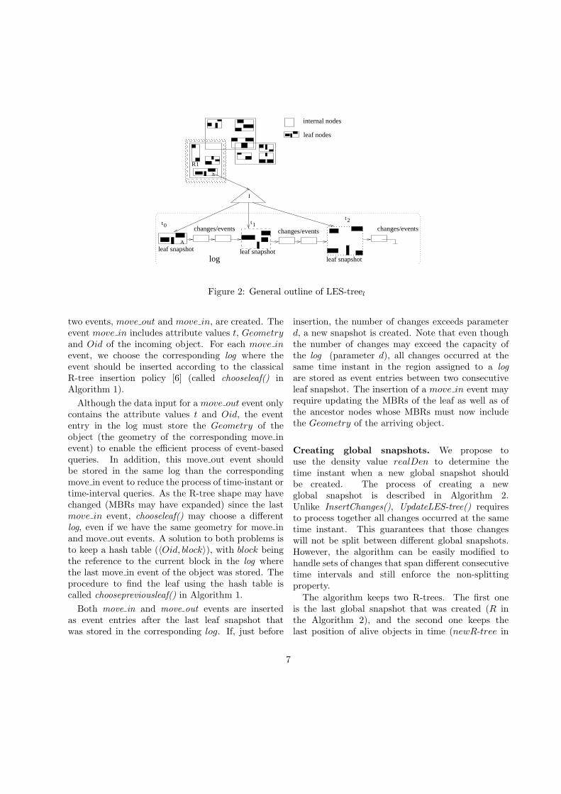
LES-treel (see Figure 2), consists of an R-tree [6]and a set of logs assigned to the regions of leavesin the R-tree. Here a log (leaf) is a structure thatstores leaf snapshots and events. In this structure,the movement of an object is not inserted directly inthe R-tree, producing the classical node splitting ofthe R-tree, but they are inserted as events in a logof an R-tree’s leaf. Figure 2 presents a region A andits corresponding log with three objects at instant

t0. At instant t1, region A has grown to include afourth object, what is reflected on the correspondingleaf snapshot. The changes that occurred between t0and t1 are stored as events in the log associated withA.

In LES-treel, areas of both the regions to whichthe logs are assigned and the MBRs of non-leaf nodesin the R-tree are always growing along time. Due tothis situation, the overlapping areas of non-leaf nodesin the R-tree increase and the efficiency of queryprocessing degrades (see Figure 2), a problem thatSection 3.2 addresses.

The LES-treel considers an R-tree [6], where theleaves are logs and these logs are linked lists of blocks.A log has two types of entries: event or change entriesand leaf snapshot entries (the first entry is alwaysa leaf snapshot). The entries in the log follow atemporal order.

An event entry is a tuple with the structure〈t,Geometry,Oid,Op〉, where t corresponds to thetime when the change occurred, and Oid is the objectidentifier. Geometry corresponds to the spatialcomponent of the object, which depends on thegeometry type (i.e., point, line, polygon or MBR)and dimension (2D or 3D). Finally, Op indicates thetype of operation (i.e., type of event or change).

This work considers only two types of events:move in (i.e, an object moves to a new location) andmove out (i.e., an object leaves its current location).Thus an object creation is modeled as a move in,an object deletion as a move out, and an objectmovement as a move out followed by a move in.The structure that stores move out entries could onlyinclude attributes t and Oid. This decreases thestorage cost of the structure, at the price of increasingthe time cost for processing queries on events (butnot the classical time-slice and time-interval queries).Later, in Section 5, we will analyze how much space(and also time) can be saved if the structure onlysupports time-slice and time-interval queries.

The second type of entry, a leaf snapshot entry,stores the snapshot of a leaf node, with one entryper each object alive at the time instant when thesnapshot was created.

Like SEST-Index [5], each LES-treel also uses aparameter d, equal for all logs in the structure,

5

S

...... ...

time

leaf snapshot

global snapshot

R−tree

t0

changes/events

logs

tn tmLES−treel

LES−tree

Figure 1: General outline of LES-tree

which represents the amount of memory, measured inthe number of blocks, used to store events betweenconsecutive leaf snapshots.

3.2 Dynamic regions

A potential problem of LES-treel is that the queryselectivity can deteriorate when regions grow due tothe arrival of new events that are stored in their logs.Remind that inserting an entry of type move in canexpand the area of MBRs, from the leaves (logs) tothe root of the tree, whereas a move out does notreduce the area of their corresponding MBR. As aconsequence of this ever growing area of MBRs, thetime cost of a spatio-temporal query (Q, t) submittedat instant t1 ≥ ts is lower than the time cost of thesame query submitted at instant t2, with t2 > t1.

To measure this effect, we define a density measureassociated with the current R-tree. This measurerealDen is defined by Eq. (1), where M is the setof MBRs located at the leaves of the R-tree, andTotalArea is the workspace area. realDen describeshow compactly the leaf MBRs cover the space, soa lower realDen value implies that the databasepoints are covered by smaller MBRs. The value ofrealDen affects the query performance, since thelarger the MBRs are, the larger is the number oflogs that must be processed to solve a query. The

value of realDen usually grows with move in events,as MBRs grow and the workspace tends to stay thesame. This explains why a query submitted at instantt1 costs less than a query submitted at instant t2,with t2 > t1.

realDen =

∑

i∈M Areai

TotalArea(1)

To solve the problem of selectivity for dynamicregions, LES-tree uses global snapshots which arecreated when the insertions of new events producesvalues of realDen (Eq. (1)) larger than a giventhreshold.

3.3 Operations and algorithms

3.3.1 Updating the structure

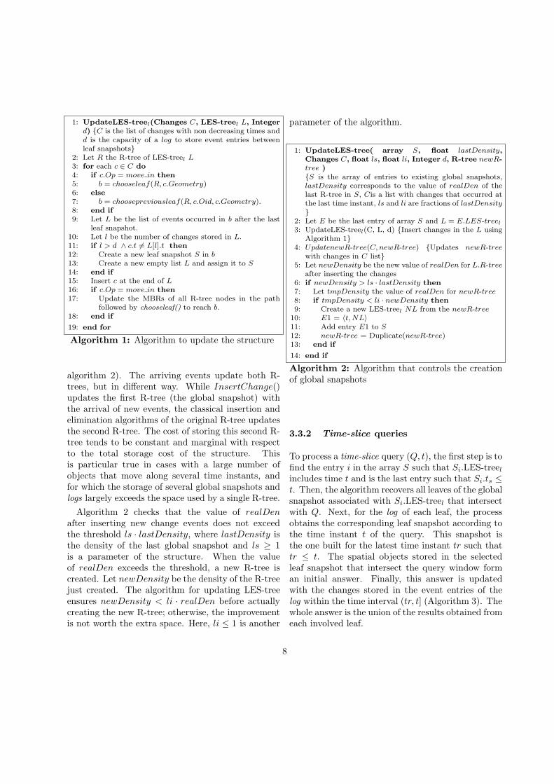
The update of LES-tree considers two algorithms.The first one (Algorithm 1) updates the LES-treel

with the arrival of new events since the time instant inwhich the global snapshots was created. The secondalgorithm (Algorithm 2) creates the global snapshots.

Updating LES-treel. This algorithms updatesthe structure upon changes that occur at each timeinstant. Let us assume that the changes to beprocessed are stored in a list. When an object moves,

6

t2

A

A

t1

I

t0

R1

changes/events changes/events changes/events

internal nodes

leaf nodes

leaf snapshot leaf snapshotleaf snapshotlog

Figure 2: General outline of LES-treel

two events, move out and move in, are created. Theevent move in includes attribute values t, Geometry

and Oid of the incoming object. For each move in

event, we choose the corresponding log where theevent should be inserted according to the classicalR-tree insertion policy [6] (called chooseleaf() inAlgorithm 1).

Although the data input for a move out event onlycontains the attribute values t and Oid, the evententry in the log must store the Geometry of theobject (the geometry of the corresponding move inevent) to enable the efficient process of event-basedqueries. In addition, this move out event shouldbe stored in the same log than the correspondingmove in event to reduce the process of time-instant ortime-interval queries. As the R-tree shape may havechanged (MBRs may have expanded) since the lastmove in event, chooseleaf() may choose a differentlog, even if we have the same geometry for move inand move out events. A solution to both problems isto keep a hash table (〈Oid, block〉), with block beingthe reference to the current block in the log wherethe last move in event of the object was stored. Theprocedure to find the leaf using the hash table iscalled choosepreviousleaf() in Algorithm 1.

Both move in and move out events are insertedas event entries after the last leaf snapshot thatwas stored in the corresponding log. If, just before

insertion, the number of changes exceeds parameterd, a new snapshot is created. Note that even thoughthe number of changes may exceed the capacity ofthe log (parameter d), all changes occurred at thesame time instant in the region assigned to a logare stored as event entries between two consecutiveleaf snapshot. The insertion of a move in event mayrequire updating the MBRs of the leaf as well as ofthe ancestor nodes whose MBRs must now includethe Geometry of the arriving object.

Creating global snapshots. We propose touse the density value realDen to determine thetime instant when a new global snapshot shouldbe created. The process of creating a newglobal snapshot is described in Algorithm 2.Unlike InsertChanges(), UpdateLES-tree() requiresto process together all changes occurred at the sametime instant. This guarantees that those changeswill not be split between different global snapshots.However, the algorithm can be easily modified tohandle sets of changes that span different consecutivetime intervals and still enforce the non-splittingproperty.

The algorithm keeps two R-trees. The first oneis the last global snapshot that was created (R inthe Algorithm 2), and the second one keeps thelast position of alive objects in time (newR-tree in

7

1: UpdateLES-treel(Changes C, LES-treel L, Integerd) {C is the list of changes with non decreasing times andd is the capacity of a log to store event entries betweenleaf snapshots}

2: Let R the R-tree of LES-treel L

3: for each c ∈ C do4: if c.Op = move in then5: b = chooseleaf(R, c.Geometry)6: else7: b = choosepreviousleaf(R, c.Oid, c.Geometry).8: end if9: Let L be the list of events occurred in b after the last

leaf snapshot.10: Let l be the number of changes stored in L.11: if l > d ∧ c.t 6= L[l].t then12: Create a new leaf snapshot S in b

13: Create a new empty list L and assign it to S

14: end if15: Insert c at the end of L

16: if c.Op = move in then17: Update the MBRs of all R-tree nodes in the path

followed by chooseleaf() to reach b.18: end if

19: end for

Algorithm 1: Algorithm to update the structure

algorithm 2). The arriving events update both R-trees, but in different way. While InsertChange()updates the first R-tree (the global snapshot) withthe arrival of new events, the classical insertion andelimination algorithms of the original R-tree updatesthe second R-tree. The cost of storing this second R-tree tends to be constant and marginal with respectto the total storage cost of the structure. Thisis particular true in cases with a large number ofobjects that move along several time instants, andfor which the storage of several global snapshots andlogs largely exceeds the space used by a single R-tree.

Algorithm 2 checks that the value of realDen

after inserting new change events does not exceedthe threshold ls · lastDensity, where lastDensity isthe density of the last global snapshot and ls ≥ 1is a parameter of the structure. When the valueof realDen exceeds the threshold, a new R-tree iscreated. Let newDensity be the density of the R-treejust created. The algorithm for updating LES-treeensures newDensity < li · realDen before actuallycreating the new R-tree; otherwise, the improvementis not worth the extra space. Here, li ≤ 1 is another

parameter of the algorithm.

1: UpdateLES-tree( array S, float lastDensity,Changes C, float ls, float li, Integer d, R-tree newR-tree ){S is the array of entries to existing global snapshots,lastDensity corresponds to the value of realDen of thelast R-tree in S, Cis a list with changes that occurred atthe last time instant, ls and li are fractions of lastDensity

}2: Let E be the last entry of array S and L = E.LES-treel

3: UpdateLES-treel(C, L, d) {Insert changes in the L usingAlgorithm 1}

4: UpdatenewR-tree(C, newR-tree) {Updates newR-tree

with changes in C list}5: Let newDensity be the new value of realDen for L.R-tree

after inserting the changes6: if newDensity > ls · lastDensity then7: Let tmpDensity the value of realDen for newR-tree

8: if tmpDensity < li · newDensity then9: Create a new LES-treel NL from the newR-tree

10: E1 = 〈t, NL〉11: Add entry E1 to S

12: newR-tree = Duplicate(newR-tree)13: end if

14: end if

Algorithm 2: Algorithm that controls the creationof global snapshots

3.3.2 Time-slice queries

To process a time-slice query (Q, t), the first step is tofind the entry i in the array S such that Si.LES-treel

includes time t and is the last entry such that Si.ts ≤t. Then, the algorithm recovers all leaves of the globalsnapshot associated with Si.LES-treel that intersectwith Q. Next, for the log of each leaf, the processobtains the corresponding leaf snapshot according tothe time instant t of the query. This snapshot isthe one built for the latest time instant tr such thattr ≤ t. The spatial objects stored in the selectedleaf snapshot that intersect the query window forman initial answer. Finally, this answer is updatedwith the changes stored in the event entries of thelog within the time interval (tr, t] (Algorithm 3). Thewhole answer is the union of the results obtained fromeach involved leaf.

8

1: time-sliceQuery(Rectangle Q, Time t, array S)2: Find the last entry i in S such that Si.ts ≤ t

3: Let R be the R-tree of Si.LES-treel.4: B = SearchRtree(Q, R) {B is the set of leaves (logs) that

intersect Q}5: G = ∅ {G is the set of objects that belong to the answer}6: for each log b ∈ B do7: Let tr be the time of the latest leaf snapshot in b such

that tr ≤ t

8: Let A be the set of all objects in the leaf snapshotcreated at time instant tr in log b and that intersectQ

9: for each event entry c ∈ b such that tr < c.t ≤ t do10: if c.Geometry intersects Q then11: if c.Op = move in then12: A = A ∪ {c.Oid}13: else14: A = A − {c.Oid}15: end if16: end if17: end for18: G = G ∪ A

19: end for

20: return G

Algorithm 3: Algorithm to process a time-slicequery

3.3.3 Time-Interval queries

Two procedures process time-interval queries(Q, [ti, tf ]). The first one (see Algorithm 4) aimsto transform (Q, [ti, tf ]) into a set of time-intervalsub-queries (Q, t1, t2), whose time intervals [t1, t2] arenon-overlapping sub-intervals of [ti, tf ]. The limitsof an interval are defined such that the sub-querycovers the time interval between consecutive globalsnapshots, with the exception that the initial instantof the first time interval must be ti, and the finalinstant of the last time interval must be tf . Theanswer of the query (Q, [ti, tf ]) is obtained by thealgorithm 5 as the union of the answers of each ofthe sub-queries.

The second procedure (see Algorithm 5) processeseach of the time-interval (Q, [t1, t2]). This algorithmstarts by finding the set of spatial objects thatintersect the query window (Q) at the initial instantt1. This is equivalent to a time-slice query at instantt1. Then, objects are updated based on the changesoccurred within the interval (t1, t2] (Algorithm 5).

1: IntervalQuery(Rectangle Q, Time ti, tf , array S)2: ANS = ∅ {Answer set}3: Find the last entry i in S such that Si.ts ≤ ti4: t1 = Si.ts5: while t1 < tf do6: if i is the last entry in S then7: t2 = tf8: else9: t2 = min(Si+1.ts, tf )

10: end if11: ANS = ANS ∪ SubIntervalQuery(Q, Time t1, t2,

Si.pLES-treel)12: t1 = t213: i = i + 114: end while

15: return ANS

Algorithm 4: Algorithm to process a time-intervalquery

3.3.4 Event queries

One of the novelties of the LES-tree structure is itscapability for processing not only time-slice and time-interval, but also queries on events. For example,given a region Q and an instant t, an event query maybe to find the number of objects that moved in or outfrom region Q at instant t. These types of queries arepossible and useful, for example, in applications thataim to analyze the pattern of objects’ movements [23,3].

Processing event queries with LES-tree (seeAlgorithm 6) is simple and efficient, since thestructure explicitly stores the changes over objects’geometry. Algorithms for these types of queriesare similar to those for time-slice and time-intervalqueries.

4 A LES-tree Cost Model

This section presents a cost model for LES-tree, which allows us to predict its storage andtime costs for spatio-temporal queries. The costmodel is experimentally validated to demonstrate itsprediction capability.

The cost model of LES-tree assumes that the initiallocations of objects and their subsequent positionsupon movements distribute uniformly and that theevents consist of random changes in objects’ location,

9

1: SubIntervalQuery(Rectangle Q, Time t1, t2, LES-treel L )

2: Let R be the R-tree of L

3: B = SearchRtree(Q, R) {B is the set of leaves (logs) thatintersect Q}

4: G = ∅ {G is the set of objects that belong to the answer}5: for each log b ∈ B do6: Let tr be the time of the latest leaf snapshot in b such

that tr ≤ t

7: Let A be the set of all objects in the leaf snapshotcreated at time instant tr in log b and that intersectQ

8: Update A with the changes stored in b occurred between(tr, t1] {like a time-slice query}

9: ts = Next(t1) {Next(x) returns the next instant afterx having changes in log b}

10: while ts ≤ t2∧ there exist unprocessed event entries inlog b do

11: for each event entry c ∈ b such that c.t = ts do12: if c.Geometry intersects Q then13: if c.Op = move in then14: A = A ∪ {c.Oid}15: else16: A = A − {c.Oid}17: end if18: end if19: end for20: let G = G ∪ {〈o, ts〉, o ∈ A}21: ts = Next(ts)22: end while23: end for

24: return G

Algorithm 5: Algorithm to process a subquery.

so the number of objects does not change along time.Figure 3 describes the variables used in the costmodel of LES-tree.

The development of the model follows two steps.First, a model for LES-treel and then its extensionto a model for LES-tree.

4.1 A cost model for LES-treel

4.1.1 Storage cost of the R-tree

Let N be the number of objects stored in an R-treewith average fanout f . The height h of an R-tree isgiven by the equation h =

⌈

logf N⌉

[17].

Since the number of entries in a node is on averagef , it is possible to assume that the number of leaf

nodes is N1 =⌈

Nf

⌉

and that the number of non-leaf

1: EventQuery(Rectangle Q, Time t, array S)2: Find the last entry i in S such that Si.ts ≤ t

3: Let R be the R-tree of Si.LES-treel.4: B = SearchRtree(Q, R) {B is the set of regions that

intersect Q}5: oi = 0 {number of objects that moved into Q at instant

t}6: oo = 0 {number of objects that moved out of Q at instant

t}7: for each log b ∈ B do8: find the first event entry c ∈ b such that c.t = t

9: while c.t = t do10: if c.Geometry intersects Q then11: if c.Op = move in then12: oi = oi + 113: else14: oo = oo + 115: end if16: end if17: c = NextChange(c) {NextChange(x) returns the

event entry following x in log b}18: end while19: end for

20: return (oi, oo)

Algorithm 6: Algorithm to process an event query

nodes at the level immediately superior to the leaves

is N2 =⌈

N1

f

⌉

. Considering that the root is at level h

and the leaves are at level 1, the average number of

nodes at level j is given by equation Nj =⌈

Nfj

⌉

[17].

Thus the average number of nodes used (i.e., storagecost) for an R-tree is determined by Eq. (2).

TN =

h∑

j=1

⌈

N

f j

⌉

≈ h +

⌊

N · (fh − 1)

fh · (f − 1)

⌋

≈ logf N +N

f(2)

4.1.2 Time cost of the R-tree

Based on [20, 17], the number of nodes accessed byan R-tree (i.e., time cost) in spatial window queries(q1, . . . , qn) is given by Eq. (3) (see next for Dj).

DAn = 1 +

h∑

j=1

N

f j.

n∏

i=1

(

(

Dj .f j

N

)

1

n

+ qi

)

(3)

10

Symbol Description

ai Length of the time interval of a query (subquery)c Changes that fit in a block (one change is equivalent to two operations, one move in plus

one move out )cc Usage average percentage of a node in an R-treeD Initial density of the set of objects

DA Average number of nodes in an R-tree accessed for a spatial queryf Average capacity of a node in an R-tree (fanout), f = cc · Mh Height of an R-treeil Number of time instants that can be stored in a log between consecutive leaf snapshotsl Total number of changes stored between consecutive leaf snapshots

igs Number of time instants between global snapshots, or how long it takes to create a newglobal snapshot

M Maximum capacity of a node in an R-tree (maximum number of entries)M1 Maximum capacity of a node in an R-tree for reaching a given densityN Total number of objectsnl Number of changes stored in a log adjusted to an integer number of time instantsnt Time instants stored in the structurep Change percentage between time instants (change frequency)q Width of the query rectangle along a dimension, as a fraction of the total space

TN Total number of blocks used by an R-treels Threshold that determines when a new global snapshot is created

NB Number of logsDAts Number of blocks accessed in a time-slice queryDAin Number of blocks accessed in a time-interval query

TBtotal Total number of blocks needed to store the LES-treel structure

Figure 3: Definition of variables

Given that our experiments consider 2-dimensionalobjects, DA = DA2 is defined by Eq. (4), assuminga square query window, q = q1 = q2.

DA = 1 +

h∑

j=1

(

√

Dj + q ·√

N

f j

)2

(4)

In Eqs. (3) and (4), Dj corresponds to the densityof spatial objects at level j [20, 17]. This is obtainedby Eq. (5), with D0 being the density of the spatialobjects that are indexed in the R-tree.

Dj =

(

1 +

√

Dj−1 − 1√f

)2

, 1 ≤ j ≤ h (5)

An important property of Eqs.(3) and (4) is thatthey depend only on f , N , q and D0 and, therefore,there is no need to construct the R-tree to estimatethe performance of the query. In this paper we haveused D0 = 0, as we index points. In general, D0 can

be computed by using Eq. (1) (i.e., D0 = realDen),where M represents the objects to be indexed.

4.1.3 Storage cost of LES-treel

Two values describe the storage cost (number ofblocks) used by the logs of LES-treel: the numberof logs and the storage needed per log. The numberof logs is equal to the number of leaves in the R-tree,

which is expressed by equation NB = N1 =⌈

Nf

⌉

.

The number of time instants (il) that can be storedbetween leaf snapshots is determined by Eq. (6).In this equation, l is the capacity of the log tostore change entries between two consecutive leafsnapshots, and p · f represents the average numberof changes that would occur in a region at each timeinstant.

il =

⌈

l

p · f

⌉

(6)

11

Using Eq. (6), it is possible to calculate the valuenl (Eq. (7)), such that all events occurred at thesame time instant are stored between the same leafsnapshots.

nl = p · f · il (7)

With il and nl, the number of blocks used per eachlog is given by Eq. (8). In this equation, the firstterm of the sum corresponds to the number of leafsnapshots. This is equal to the number of blocks usedby a leaf snapshot if we assume that the alive objectsfit, on average, in a disk block (as it initially happensin the R-tree leaves). The second term represents thenumber of blocks required, on average, for each logto store all the changes occurred at all time instantsexcept those after the last leaf snapshot. The lastterm is the number of blocks occupied for storing thechanges occurred after the last leaf snapshot.

TBlog =

⌈

nt

il

⌉

+

(⌈

nt

il

⌉

− 1

)

·⌈

nl

c

⌉

+

⌈(

nt

il−⌊

nt

il

⌋)

· nl

c

⌉

(8)

Finally, the number of blocks used by the LES-treel

is given by Eq. (9).

TBtotal = (TN − NB) + NB · TBlog

≈ logf N + N · nt · p(

1

l+

1

c

)

(9)

The latter approximation is meant to give intuitionon the result, and not replace the exact formula. Theexperimental validation of the model uses the exactformula of TBtotal, not the approximation.

4.1.4 Time cost of LES-treel

The time cost of LES-treel can be estimated byadding the time cost of accessing the R-tree withoutleaves and the time cost of processing all logs thatintersect the query window. In the following, Rp-tree refers to the R-tree without leaf nodes. The leafnodes of the Rp-tree contain the MBRs for each ofthe leaf nodes in the R-tree.

The number of objects handled by the Rp-tree isNp = N

f. Let hp =

⌈

logf Np

⌉

= h − 1 be the heightof the Rp-tree. The number of nodes accessed in thetree is given by Eq. (10).

DARp−tree = 1 +

hp∑

j=1

(

√

Dj+1 + q ·√

Np

f j

)2

= DA −(

√

D1 + q ·√

N

f

)2

(10)

In Eq. (10), we use Dj+1 because the objects in theRp-tree are the leaves of the R-tree. The number oflogs to be processed in a query depends strongly onthe density formed by the MBRs of the leaves andquery. This number of logs is defined in Eq. (11),

where D1 =

(

1 +√

D0−1√f

)2

.

NL =

(

√

D1 + q ·√

N

f

)2

(11)

Therefore, the number of blocks accessed in a time-slice query is defined by Eq. (12).

DAts = DARp−tree + NL ·(

1 +

⌈

nl

2 · c

⌉)

≈ q2 · N

f·(

1 +l

2 · c

)

(12)

Likewise, the average number of blocks accessed in atime-interval query is given by Eq. (13).

DAin = DAts + NL ·⌈

(ai − 1) · p · fc

⌉

≈ q2 · N

f·(

1 +l2

+ ai · p · fc

)

(13)

Again, the approximations for DAts and DAin justserve to give intuition and do not replace the exactformulas.

Based on the cost model for time-slice and time-interval queries, we can derive the cost of processingqueries on events, since these queries also considertemporal and spatial windows.

12

4.1.5 Experimental validation of the cost

model for LES-treel

In order to evaluate the cost model, severalexperimental evaluations were conducted withsynthetic data obtained from GSTD [19]. Theseexperiments used 23,268 objects (points) and 200time instants with change frequencies of 1%, 5%,10%, 15%, 20% and 25%. They also consideredvalues of the parameter d equal to 2, 4 and 8 blocks,where l = d · c (we consider c = 21 changes in ourexperiments). The value f of the R-tree was set to34 (68% of the capacity [17] of a node in an R*-treethat is able to hold 50 entries).

Figures 4, 5 and 6 evaluate the predictioncapability of the cost model for both storage and timerequirements. Figure 4 shows that the storage costpredicted by the model and the one obtained with theexperiments are similar for all values of d analyzed,with a relative average error of 15%.

Figures 5 and 6 show that the prediction of thetime cost of the query processing is very good, witha relative average error of 8%.

4.2 A cost model for LES-tree

This section describes the storage and time costs ofLES-tree. The idea of the global snapshots is to keepa stable performance of the structure along time,since the performance decreases as consequence ofthe increasing density of the initial R-tree. The costmodel assumes objects uniformly distributed over thespace and the same density of the R-tree in eachglobal snapshot. Another important consideration isthat, with the purpose of capturing the evolution ofthe MBRs’ density, the operations of type move in

are modeled as insertions in an R-tree. Finally, weassume a constant number of objects along time.

To incorporate the effect of the global snapshotsin the basic model for LES-treel, it is necessary toestimate how many global snapshots (ngs) shouldbe created. To do so, we estimate the number ofobjects (M1) that must be stored in each leaf nodein order to reach the density threshold D′

1 = ls · D1,where D1 is the initial density of the R-tree and D′

1 isthe density value that triggers the creation of a new

global snapshot.

Given f = cc · M and Eq. (5), Eq. (14) estimatesthe density of the MBRs of the leaves in the R-tree.

D1 =

(

1 +

√D0 − 1√cc · M

)2

(14)

Thus, it is possible to obtain M1 by Eq. (15).

(

1 +

√D0 − 1√cc · M1

)2

= ls ·(

1 +

√D0 − 1√cc · M

)2

(15)

From Eq. (15), M1 can be expressed by Eq. (16).

M1 =

(√D0 − 1

)2

cc ·(√

ls ·(

1 +√

D0−1√cc·M

)

− 1)2

(16)

As it was mentioned before, the value of M1

indicates how many events should be inserted toreach density D′

1. With M1, it is possible to obtainthe time interval between global snapshots (igs). Todo so, we obtain the total number objects stored inthe R-tree when the number of objects in the leafnodes of the R-tree reaches M1. This is M1 · N

cc·M ,

where Ncc·M is the number of leaves (or logs) in the

original R-tree. Therefore, the number of changesthat should be inserted in the R-tree to reach densityD′

1 is calculated as M1 · Ncc·M − N . The estimated

number of objects inserted in the R-tree in every time

instant is N · p, and therefore, igs =⌈

M1· Ncc·M

−N

N ·p

⌉

is the number of time instants that are stored in alog before a new global snapshot is created. This issimplified to obtain Eq. (17).

igs =

⌈

M1

cc·M − 1

p

⌉

(17)

For example, if cc = 0.68, N = 20, 000, M = 50,ls = 1.3, p = 0.10 and D0 = 0, the values of M1

and igs are approximately 480 and 132, respectively,which implies that every 132 time instants we needto create a new global snapshot.

13

0 10 20 30 40 50 60 70 80 90

100

0 5 10 15 20 25

MB

ytes

change frequency(%)

ExperimentalModel

0 10 20 30 40 50 60 70 80 90

0 5 10 15 20 25

MB

ytes

change frequency(%)

ExperimentalModel

0 10 20 30 40 50 60 70 80

0 5 10 15 20 25

MB

ytes

change frequency(%)

ExperimentalModel

d = 2 d = 4 d = 8

Figure 4: Estimation of the storage use for a LES-treel

10 20 30 40 50 60 70 80 90

100

0 10 20 30 40 50 60 70 80

read

blo

cks

length of time interval

ExperimentalModel

20 30 40 50 60 70 80 90

100 110

0 10 20 30 40 50 60 70 80

read

blo

cks


ExperimentalModel

30 40 50 60 70 80 90

100 110 120

0 10 20 30 40 50 60 70 80

read

blo

cks


ExperimentalModel

d = 2 d = 4 d = 8

Figure 5: Estimation of the time cost of queries by LES-treel (10% change frequency and 6% in eachdimension for the query window)

4.2.1 Storage cost of LES-tree

Having igs, the estimation of the storage cost forLES-tree is simple, since it is enough to consider thatthe number of global snapshots is equal to ngs =⌈ nt

igs⌉. Each global snapshot should store the changes

occurred along igs time instants. In addition, the lastglobal snapshot should store the changes occurredalong lt = nt−igs·⌊ nt

igs⌋ time instants. Using Eq. (9),

and replacing TBlog by TBigslog or TBlt

log, we obtainthe storage used by the logs in each global snapshot.TB

igslog is obtained from Eq. (8) by replacing nt by igs,

and TBltlog by replacing nt by lt. Thus, the storage

cost of LES-tree is defined by Eq. (18).

TBGStotal =

⌊

nt

igs

⌋

·(

(TN − NB) + NB · TBigslog

)

+ (TN − NB) + NB · TBltlog (18)

4.2.2 Time cost of LES-tree

Clearly, the cost model defined by Eq. (12) for time-slice queries does not change, because to process aquery of this type only needs to access a single LES-treel. For time-interval queries, we first need to knowthe number of global snapshots (i.e., the numberof LES-treel) that the algorithm of a time intervalquery should access.The estimated number of globalsnapshots that a query with a time interval of ai

intersects is defined by Eq. (19).

ngsi =

⌈

ai

igs

⌉

(19)

The length of the interval ai is transformed into

14

0

10

20

30

40

50

60

70

2 4 6 8 10 12

read

blo

cks

% of dimension in each axis

ExperimentalModel

10

20

30

40

50

60

70

80

90

2 4 6 8 10 12

read

blo

cks


ExperimentalModel

0

20

40

60

80

100

120

2 4 6 8 10 12

read

blo

cks


ExperimentalModel

d = 2 d = 4 d = 8

Figure 6: Estimation of the time cost of queries by LES-treel (10% change frequency and time interval lengthequal to 10)

a set of ni =⌊

aiigs

⌋

intervals of length igs plus

an additional interval of length lr = ai − ni · igs.Thus, to determine the time cost of LES-tree, a time-interval query is decomposed into ni queries withtime intervals of length igs and a query with timeinterval of length lr. For each R-tree, the density ofleaves’ MBR is at worst D′

1 = ls · D1 and, therefore,the number of logs that the spatial component of thequery will intersect is given by Eq. (20).

NL =

(

√

D′1 + q ·

√

N

cc · M

)2

(20)

Finally, replacing ai by igs (to obtain DAigsin ) or

lr (to obtain DAlrin) in Eq. (13), we can obtain the

number of blocks accessed by LES-tree in a spatio-temporal query (Eq. (21)).

DASGin = ni · DAigsin + DAlr

in (21)

4.2.3 Experimental validation of the cost

model of LES-tree

In order to evaluate the cost model, new experimentalevaluations were conducted with synthetic dataobtained from GSTD [19]. These experiments used23,268 objects (points) and 200 time instants withchange frequency of 5% and 10%, and 4 blocks forparameter d. The experiment considered values ofthe threshold (ls) from 1.1 to 1.35. Figure 7 shows

that the prediction of the storage cost is very good,with a relative average error of 14%. The modelestimates the time cost of query processing with arelative average error of 14% (see Figures 8 and 9).Note that in Figure 8 the use of global snapshotsappears to be counterproductive. This is becausewe purposely used ls values lower than advisablein order to obtain a clear difference with respectto the standard structure. As the distribution isuniform, a correct parameterization (such as ls =1.20) would recommend very few global snapshotsand the difference with the standard structure wouldbe negligible. The use of global snapshots isadvantageous when the data does not distributeuniformly, as shown in Section 5.2.

Our model turns also to be useful on nonuniformdata. The reason is that the global snapshottechnique, in some sense, makes the structure behaveover nonuniform data in a way similar to uniformdata. To adapt our model to an arbitrary initialdistribution, we only have to compute the initialdensity and global snapshot rate according to thereal data. For the density, instead of using Eq. 14,we must build the R-tree for the spatial data athand, and use the MBRs M of the leaves tocompute D1, as realDen of Eq. (1). For the globalsnapshot rate we need to compute M1 for arbitrarydistributions. We replace the analytic formula ofEq. (16) by a procedure that builds R-trees overthe initial data using increasing node capacities until

15

0

5

10

15

20

25

30

1.1 1.15 1.2 1.25 1.3 1.35

Mby

tes

threshold(%)

ExperimentalModel

0

10

20

30

40

50

60

1.1 1.15 1.2 1.25 1.3 1.35

Mby

tes

threshold(%)

ExperimentalModel

5% change frecuency 10% change frecuency

Figure 7: Estimation of the storage used for LES-tree

the density reaches a value D′1 = ls · D1. This is

all the computation we need over the real data (nosimulations over query streams nor change events, forexample). All the rest of the formulas of the modelcan be used unaltered once D1 and M1 are obtained.

An experimental validation of our model in ascenario with non uniform distribution of objectsand global snapshots uses the same data set of theevaluation of MVR-tree in [16]. Such data set consistsof 23,268 objects (points) that moves with 10% ofchange frequency during 199 time instants. We referto this data set as NUD (Figure 10).

In Figure 11 we compare the experimental behaviorover the NUD data with our model. It can beseen that our model, although designed for uniformdistributions, accurately predicts the behavior of thestructure on nonuniform data as well. The spacerequired is accurately predicted as well: the error istypically very low (e.g. 3% for ls = 1.3). For verylow ls the space required can get larger (e.g. 20% forls = 1.10), but those low ls values are not of use inpractice.

0

50

100

150

200

30 40 50 60 70 80

read

blo

cks


Experimental (using ls = 1.30)Model (using ls = 1.30)

Experimental (using ls = 1.10)Model (using ls = 1.10)

Figure 11: Estimation of the time cost of LES-treefor the data set NUD (change frequency = 10%, and6% in each dimension of the spatial window)

5 Experimental evaluation

This section presents an experimental evaluationthat compares LES-tree with respect to SEST-Index and MVR-tree. The evaluation considers twoscenarios with the same number of objects (23,268points) and time instants stored in the database.While in the first scenario objects initially distribute

16

0

50

100

150

200

250

30 40 50 60 70 80

read

blo

cks


Experimental(using ls = 1.05)Model(using ls = 1.05)


Experimental(without global snapshot)Model(without global snapshot)

0

50

100

150

200

250

30 40 50 60 70 80

read

blo

cks

length of temporal interval



Experimental(without global snapshot)Model(without global snapshot)

(a) 5% change frequency (b) 10% change frequency

Figure 8: Estimation of the efficiency of the queries processed with LES-tree and uniform distribution (spatialrange of the queries made up of 6% of each dimension).

uniformly over the space, in the second scenarioobjects present the non-uniform initial distributionshown in Figure 10.

5.1 Evaluation of LES-tree with uni-

form distribution of objects

All experiments in this section consider a densitythreshold value of 30% to create new globalsnapshots. With this value, we create only one globalsnapshot. A stricter value of this density threshold(i.e., a value less than 30%) creates unnecessaryglobal snapshots. As we will see later, the advantageof using global snapshots is reflected in the evaluationof LES-tree with data of a non-uniform distributionof objects (see Figure 10).

A first experimental evaluation compares LES-tree with SEST-Index and MVR-tree. It comparesstorage and time costs of all methods when processingspatio-temporal queries. After the initial uniformdistribution of objects, objects change their positionsover 200 time instants. The set of objects wasobtained with the spatio-temporal data generatorGSTD [19].

The evaluation uses different lengths of thelogs that store events, that is, different values of

parameter d (see Figure 3) for the structures SEST-Index and LES-tree. Such lengths are determined interms of the number of events that occur in 1, 12and 24 time instants. For example, if we considerthe number of events that occur at 1 time instantfor 23,268 objects with 10% of change frequency,the value of d is 1 for LES-tree and 56 for SEST-Index. Note that by keeping logs that store only theevents occurr at 1 time instant, both LES-tree andSEST-Index reach the best performance for queryprocessing, to the price of the largest storage cost.

For SEST-Index, the value d is obtained with theexpression d = p·N ·k

c, where k represents the number

of time instants (i.e., 1,12 or 24) for which changes arestored in the logs. Likewise, for LES-tree the value d

is obtained by the equation d = p·f ·kc

, where d,N, c

and f are defined in Figure 3.

5.1.1 Storage cost

Figure 12 shows the storage cost of MVR-tree, SEST-Index and LES-tree for different values of changefrequency. In the case of LES-tree and SEST-Index,as d increases, the storage cost reduces. In Figure 12we can observe that LES-tree requires approximatelythe same storage than MVRT-tree with a parameter d

17

0

50

100

150

200

250

2 4 6 8 10 12

read

blo

cks


ExperimentalModel

0

50

100

150

200

250

2 4 6 8 10 12

read

blo

cks


ExperimentaModel

(a) 5% change frequency (b) 10% change frequency

Figure 9: Estimation of the efficiency of the queries processed with LES-tree considering uniform distribution(length of temporal interval equal to 40 units and ls = 1.1).

(a) (b) (c)

Figure 10: Data of moving objects: (a) instant 1, (b) instant 100 and (c) instant 199

for storing 1 time instant. Remember that, in termsof storage cost, this is the worst scenario for LES-tree. LES-tree, however, overcomes MVR-tree withincreasing values of d. For example, if we consider10% change frequency and values of d equal to 1 and4, LES-tree requires, approximately, 78% and 65% ofthe storage of MVR-tree, respectively. For the samechange frequency and values of d equal to 560 and1,120, SEST-Index requires less storage than MVR-tree and LES-tree; however, and as we will show later,the performance of SEST-Index is worse than theperformance of LES-tree and MVR-tree.

5.1.2 Time-slice and time-interval queries

Figures 13, 14 and 15 show the performance of MVR-tree, SEST-Index and LES-tree to process spatio-temporal queries (Q, [ti, tf ) that consider differentlengths for time intervals [ti, tf ] and different areas forQ. In Figure 13 we can see that LES-tree overcomesby far SEST-Index. Note that this figure only showsthe best scenarios of SEST-Index, that is, d = 56for 10% change frequency and d = 25 for 5% changefrequency, and where its storage is larger than thestorage of LES-tree (for d = 1, d = 2 y d = 4) andMVR-tree.

The unfavorable performance of the SEST-Index

18

change MVR-tree / LES-tree SEST-Indexfrequency MV3R-tree 1 12 24 1 12 24

(%) (Mb) d (Mb) d (Mb) d (Mb) d (Mb) d (Mb) d (Mb)

1 6 / 6.3 1 5 1 5 1 5 6 55 55 10 110 65 26 / 26.5 1 19 1 19 2 16 25 59 270 14 540 1010 46 / 46.8 1 36 2 29 4 24 56 64 560 19 1120 1515 66 1 55 3 38 6 35 75 68 750 25 1500 2020 81 1 74 4 47 8 43 102 73 1000 30 2000 2525 101 1 94 5 56 10 52 126 78 1250 35 2500 30

Figure 12: Storage space for MV-tree, LES-tree and SEST-Index (d is the number of blocks used to storechanges)

with respect to LES-tree is explained by two factors:

i) The SEST-Index duplicates all the objects ineach snapshot including those without changes.The problem of duplication could, in principle,be solved by using the overlapping strategy ofHR-tree, but the experimental results showedthat there is a low saving in storage, around5% – 7%. Instead, LES-tree builds a new globalsnapshot only for the leaves that have undergoneseveral changes.

ii) The SEST-Index groups the changes only inrelation to time, and not in relation to time andspace as does LES-tree. All changes that occurbetween consecutive leaf snapshots are stored ina single log, which may span many disk blocks.In a query (Q, t), Q is used only for getting theinitial set of objects, but not for filtering thelog blocks in the subsequent processing. Thus,all events between the time of the leaf snapshotand the query time t are processed. This can bealleviated by enforcing short logs (with a smalld), but this exacerbates problem a).

In Figure 13, LES-tree overcomes MVR-tree for allvalues of d considering 5% and 10% change frequency.Even for the worst scenarios of LES-tree to evaluatequeries (d = 2 for 5% frequency and d = 4 for10% change frequency), the performance of LES-tree is better than the performance of MVR-tree, adifference that increases with the length of the query

time interval. Recall that for these scenarios, LES-tree requires less storage than MVR-tree.

Figures 14 and 15 show the behavior of MVR-tree,SEST-Index and LES-tree for time-interval queriesfor which the temporal interval lengths were 1 and4, and the spatial range was made up of 2% –20% from each dimension. In Figure 14 (time-slice query) with d = 1, LES-tree overcomes MVR-tree for all the areas of query window. In thisscenario, both structures use approximately the samestorage. In the same figure, SEST-index overcomesLES-tree as the area of the query window increases.For example, in Figure 14-a (5% change frequency),SEST-Index starts to outperform LES-tree from anarea made up of 14% of each dimension for d = 1.In contrast, for 10% change frequency, SEST-Indexpresents better performance than the performanceof LES-tree starting from areas covering 20% ofeach dimension. SEST-Index, however, requires 3times and twice the space than LES-tree for changefrequency of 5% (d = 24) and 10% (d = 56),respectively. The experiment also shows that the areaof the queries when SEST-Index outperforms LES-tree increases as the temporal interval length enlarge.The latter can be seen in Figure 15 where LES-treeovercomes easily MVR-tree and SEST-Index for allareas of query window and values of d = 1 and d = 2for LES-tree.

There exists a spatio-temporal access methodknown as MV3R-tree [15] that corresponds to a

19

0

50

100

150

200

250

300

0 2 4 6 8 10 12 14 16 18 20

read

blo

cks


MVR-treeMV3R-tree

SEST-Index(d=25)LESTR-tree(d=1)LESTR-tree(d=2)

0

50

100

150

200

250

300

350

400

0 2 4 6 8 10 12 14 16 18 20

read

blo

cks


MVR-treeMV3R-tree

SEST-Index(d=25)LESTR-tree(d=1)LESTR-tree(d=2)LESTR-tree(d=4)

(a) 5% change frecuency (b) 10% change frecuency

Figure 13: Blocks read by MVR-tree, SEST-Index and LES-tree for queries with different temporal intervallengths (10% change frequency and spatial range made up of 6% of the length of each dimension).

variant of MVR-tree. MV3R-tree combines MVR-tree with a small 3D R-tree1[15]. MVR-tree solvesqueries with short temporal intervals, whereas 3D R-tree solves queries with long temporal intervals. In[15], MV3R-tree, HR-tree [10, 11], and the original3D R-tree are compared2[21]. The results show thatthe 3D R-tree used by MV3R-tree requires only 3%of the storage used by MVR-tree (thus MV3R-treeis only 3% larger than MVR-tree). MV3R-tree uses1.5 times the storage required by the original 3DR-tree, and MV3R-tree needs a minimum fractionof the HR-tree storage. On the other hand, ourexperiments show that LES-tree requires, in average,approximately 75% of the storage used by MVR-tree, considering all changes occurred in 12 timeinstants. Thus, we can state that LES-tree needsapproximately the same storage than 3D R-tree.

With respect to the queries with short temporalintervals (less than 5% of the total of the temporalintervals of the database), MV3R-tree uses a MVR-tree to evaluate them. In our experiments, data

1This 3D R-tree is created considering the leaves of a MVR-tree; that is, each leaf of the MVR-tree is an object in the 3DR-tree

2In constrast, this 3D R-tree stores each object instead ofeach leaf of the MVR-tree

contains 200 snapshots and, therefore, LES-tree willoutperform the MV3R-tree in the same situationswhere we considered temporal intervals less than orequal to 10 time units. For queries that consider atemporal interval whose length is larger than 5%,MVR-tree needs to do approximately between 75%and 80% of the accesses required by MVR-tree asis shown in [13]. Assuming that the cost (time) ofMV3R-tree will be 75% of MVR-tree, it is possibleto affirm that LES-tree is always better than MV3R-tree for queries whose temporal interval is larger than2 time units (for d = 4 and change frequency of 10%representing the worst scenario of LES-tree).

It is also possible to conclude that LES-tree isbetter than the spatio-temporal access method thatuses the original 3D R-tree, given that the results in[15] show that 3D R-tree does not outperform MV3R-tree in none of the analyzed situations. In querieswith long temporal intervals, 3D R-tree experimenteda performance very similar to that of MV3R-tree.

LES-tree is an event-oriented access method thataims to efficiently process not only time-slice andtime-interval queries, but also queries on events. Toguarantee performance for all queries, the structuremaintains some attributes that can be eliminatedif we are only interested in time-slice or time-

20

0

50

100

150

200

2 4 6 8 10 12 14 16 18 20

read

blo

cks

% of the dimension in each axis

MVR-treeMV3R-tree


0

50

100

150

200

2 4 6 8 10 12 14 16 18 20

read

blo

cks


MVR-treeMV3R-tree


(a) 5% change frecuency (b)10% change frecuency

Figure 14: Blocks read by MVR-tree, SEST-Index and LES-tree for time-slice queries (temporal intervallength = 1) in different spatial ranges.

interval queries. More specifically, it is possible toeliminate the Geometry attribute in the move out

type event and still achieve a better performancein the processing of time-slice and time-intervalqueries. We evaluated the performance of LES-treeconsidering these modifications in the data structure(adjusted LES-tree). The results show that for 10%change frequency and d = 4, LES-tree requiresapproximately 67% of the storage required by theoriginal LES-tree and 70% of the time to processqueries whose query space window covers 6% in eachdimension and whose lengths of time intervals gofrom 1 to 20 units.

5.1.3 Queries on events

As we explained above, SEST-Index and LES-treealso enable to process queries about events thatoccurred in time instants or time intervals. Theprocessing cost of this type of queries with LES-tree is the same as the one needed for the time-slice and time-interval queries. For SEST-Index,however, it is possible to have advantages to processevent queries. We evaluate both structures with 10%change frequency and parameter d such that bothstructures require the same storage. To fulfill this

constraint, d was set to 816 and 4 for SEST-Indexand LES-tree, respectively. In this scenario SEST-Index overcomes LES-tree when the query windowcovers an area formed by more than 11% of eachdimension. SEST-Index, however, presents a poorperformance for time-slice and time-interval querieswith respect to LES-tree. For example, a time-slicequery with LES-tree requires approximately 8% ofthe time needed with SEST-Index.

Despite the fact that MVR-tree does not providean algorithm to solve queries about events, it may bepossible to process events queries. For example, anevent query can be “find how many objects enter aregion (Q) at a time instant t.” To process this querywith MVR-tree, two time-slice queries are needed:one at time instant t and the other one at the instantimmediately before t (t′). Objects that enter Q at t

correspond to those that were not found in Q in t′,but are now found in Q at t. The cost of processingthis query with MVR-tree has the double cost ofprocessing a time-slice query. Indeed, for the abovequery with a region covering 6% of each dimension,10% change frequency, and d = 4, LES-tree requiresaccess only 43% of the nodes or blocks accessed byMVR-tree.

21

0

50

100

150

200

250

300

350

400

2 4 6 8 10 12 14 16 18 20

read

blo

cks


MVR-treeMV3R-tree


0

50

100

150

200

250

300

350

400

2 4 6 8 10 12 14 16 18 20

read

blo

cks


MVR-treeMV3R-tree


(a) 5% change frecuency (b) 10% change frecuency

Figure 15: Blocks read by MVR-tree, SEST-Index and LES-tree for queries in different spatial ranges(temporal interval length = 4).

5.2 Evaluation of LES-tree with non-

uniform data distribution

This section compares LES-tree with global snap-shots against MVR-tree by using NUD data set(defined in Section 4.2.3). To obtain the storage andtime costs of queries, we use the implementation ofMVR-tree and LES-tree, this last with d = 4.

Figure 16 shows the values of density realDen

under five different scenarios: (1) the densityobtained with LES-tree, 23,268 objects (points), andan initial uniform distribution; (2) the density ofLES-tree with the set of objects NUD without globalsnapshots; (3), (4) and (5) densities of LES-tree whenconsidering the set of objects NUD, li = 1, andthresholds equal to ls = 1.3, ls = 1.6, and ls = 1.8,respectively.

The space used by LES-tree when consideringthresholds ls = 1.3, ls = 1.6, and ls = 1.8 was33Mb, 29Mb, and 28Mb, respectively, against 46Mb required by MVR-tree and 24 Mb required bythe LES-tree without global snapshots. Figure 16indicates that, when considering a threshold ls = 1.6,two global snapshots are created (approximately attime instants 10 and 50). This produces an importantimprovement on the density, reaching values that

are similar to those of scenario (1). Similar resultsare obtained with a threshold ls = 1.3. With athreshold ls = 1.8 in scenario (5), however, thedensity continues being larger than in scenario (1),affecting negatively the time cost of LES-tree.

0.2

0.4

0.6

0.8

1

1.2

1.4

0 20 40 60 80 100 120 140 160 180 200

dens

ity

time

(1) Uniform distribution(2) Non-uniform initial distribution

(3) Using ls = 1.3(4) Using ls = 1.6(5) Using ls = 1.8

Figure 16: Density for logs of LES-tree

Figure 17 shows the query performance of MVR-tree and LES-tree in scenarios (1) to (5) (in additionto the performance of MVR-tree using NUD data).

In this Figure it is possible to observe that with ls=

22

1.3 or ls=1.6, LES-tree, with global snapshots, showsa similar performance that the LES-tree withoutglobal snapshots, considering objects (23,268 points)with uniform distribution. Also, LES-tree with ls =1.3 or ls = 1.6 overcomes MVR-tree in almost all timeintervals evaluated. The advantage of LES-tree overMVR-tree in this scenario (non uniform distribution)to process queries increases drastically as the valueof d decreases and we use the adjusted LES-tree asdescribed before.

0

20

40

60

80

100

0 5 10 15 20 25

read

blo

cks


(1) Uniform distribution(2) Non-uniform initial distribution

(3) Using ls = 1.3 (4) Using ls = 1.6 (5) Using ls = 1.8 MVR-tree (NUD)

Figure 17: Query performance of LES-tree withglobal snapshots and MVR-tree over the set ofobjects con distibucion uniforme y no uniforme(NUD)

6 Conclusion and future work

This work proposes a new spatio-temporal accessmethod, LES-tree, that handles events and snapshotsassociated with space partitions. Based on theexperimental results, LES-tree (with parameter d =4) requires around 64% of the space used by MVR-tree, the best alternative structure up to date. Onthe other hand, LES-tree outperforms the MVR-treefor time-slice and time-interval queries. Unlike otherproposed spatio-temporal access methods, it is alsopossible to process queries about events using LES-tree with a similar efficiency as the algorithms used toprocess time-slice and time-interval queries. In this

paper we also described and validated a cost modelfor LES-tree. This model enables to estimate thestorage and the efficiency of the queries processedwith LES-tree (with and without global snapshots),and with a relative average error of about 15% forstorage and 11% for queries.

Besides traditional time-slice and time-interval, aswell as queries on events, LES-tree could be used forother types of queries, such as queries that specifya spatio-temporal pattern as a sequence of distinctspatial predicates in temporal order [7], calledspatio-temporal pattern queries (STP). LES-tree canefficiently process STP queries because a log in thestructure keeps the information about the moment inwhich an object enters and leaves its assigned spacepartition. Algorithms and experimental evaluationsfor these type of queries have been left out of thescope of this paper.

In addition, we are developing a method to obtainthe values of the parameters for LES-tree such thatthe structure is optimized with respect to pre-definedconstraints for storage or time cost. We also plan toinclude in the cost model the effect of using a bufferfor caching blocks or pages of the structure. Finally,we are studying new algorithms for joins and nearest-neighbor queries.

References

[1] Becker, B., Gschwind, S., Ohler, T., Seeger,B., Widmayer, P.: An asymptotically op-timal multiversion B-tree. The VLDBJournal 5(4), 264–275 (1996). DOIhttp://dx.doi.org/10.1007/s007780050028

[2] Cole, S.J., Hornsby, K.: Modeling noteworthyevents in a geospatial domain. In: M.A.Rodrıguez, I.F. Cruz, M.J. Egenhofer, S. Lev-ashkin (eds.) GeoSpatial Semantics, First Inter-national Conference, GeoS, 2005, Mexico City,Mexico, November 29-30, 2005, Proceedings,Lecture Notes in Computer Science, vol. 3799,pp. 77–89. Springer (2005)

[3] Galton, A., Worboys, M.F.: Processes andevents in dynamic geo-networks. In: M.A.

23

Rodrıguez, I.F. Cruz, M.J. Egenhofer, S. Lev-ashkin (eds.) GeoSpatial Semantics, First Inter-national Conference, GeoS, 2005, Mexico City,Mexico, November 29-30, 2005, Proceedings,Lecture Notes in Computer Science, vol. 3799,pp. 45–59. Springer (2005)

[4] Gupta, A., Mumick, I.S.: Maintenance of mate-rialized views: Problems, techniques and appli-cations. IEEE Quarterly Bulletin on Data En-gineering; Special Issue on Materialized Viewsand Data Warehousing 18(2), 3–18 (1995). URLciteseer.ist.psu.edu/gupta95maintenance.html

[5] Gutierrez, G., Navarro, G., Rodrıguez, A.,Gonzalez, A., Orellana, J.: A spatio-temporal access method based on snapshotsand events. In: Proceedings of the 13thACM International Symposium on Advances inGeographic Information Systems (GIS’05), pp.115–124. ACM Press (2005)

[6] Guttman, A.: R-trees: A dynamic indexstructure for spatial searching. In: ACMSIGMOD Conference on Management of Data,pp. 47–57. ACM (1984)

[7] Hadjieleftheriou, M., Kollios, G., Bakalov, P.,Tsotras, V.J.: Complex spatio-temporal patternqueries. In: Proceedings of the 31st internationalconference on Very large data bases (VLDB ’05),pp. 877–888. VLDB Endowment (2005)

[8] Kollios, G., Tsotras, V.J., Gunopulos, D.,Delis, A., Hadjieleftheriou, M.: Indexinganimated objects using spatio-temporal accessmethods. Knowledge and Data Engineer-ing 13(5), 758–777 (2001). URL cite-seer.nj.nec.com/494812.html

[9] Kollios, G.N.: Indexing problems in spatiotem-poral databases. Ph.D. thesis, PolytechnicUniversity, New York (2000)

[10] Nascimento, M.A., Silva, J.R.O., Theodoridis,Y.: Access structures for moving points. Tech.Rep. TR–33, TIME CENTER (1998). URL cite-seer.nj.nec.com/article/nascimento98access.html

[11] Nascimento, M.A., Silva, J.R.O., Theodoridis,Y.: Evaluation of access structures for discretelymoving points. In: Proceedings of theInternational Workshop on Spatio-TemporalDatabase Management (STDBM ’99), pp. 171–188. Springer-Verlag, London, UK (1999)

[12] Pfoser, D., Tryfona, N.: Requirements,definitions, and notations for spatio-temporalapplication environments. In: Proceedingsof the 6th ACM International Symposium onAdvances in Geographic Information Systems(GIS’98), pp. 124–130. ACM Press (1998). DOIhttp://doi.acm.org/10.1145/288692.288715

[13] Tao, Y., Papadias, D.: MV3R-tree: A spatio-temporal access method for timestamp andinterval queries. Tech. Rep. HKRUST-CS00-06,Department of Computer Science, Hong KongUniversity of Science Technology, Hon Kong(2000)

[14] Tao, Y., Papadias, D.: Efficient historical R-tree. In: SSDBM International Conference onScientific and Statical Database Management,pp. 223–232 (2001)

[15] Tao, Y., Papadias, D.: MV3R-tree: A spatio-temporal access method for timestamp andinterval queries. In: Proceedings of the27th International Conference on Very LargeData Bases, pp. 431–440. Morgan KaufmannPublishers Inc., San Francisco, CA, USA (2001)

[16] Tao, Y., Papadias, D., Zhang, J.: Costmodels for overlapping and multiversionstructures. ACM Trans. DatabaseSyst. 27(3), 299–342 (2002). DOIhttp://doi.acm.org/10.1145/581751.581754

[17] Theodoridis, Y., Sellis, T.: A model forthe prediction of R-tree performance. In:Proceedings of the fifteenth ACM SIGACT-SIGMOD-SIGART symposium on Principles ofdatabase systems (PODS ’96), pp. 161–171.ACM Press, New York, NY, USA (1996). DOIhttp://doi.acm.org/10.1145/237661.237705

24

[18] Theodoridis, Y., Sellis, T.K., Papadopoulos,A., Manolopoulos, Y.: Specificationsfor efficient indexing in spatiotemporaldatabases. In: IEEE Proceedingsof the 10th International Conferenceon Scientific and Statistical DatabaseManagement, pp. 123–132 (1998). URL cite-seer.nj.nec.com/theodoridis98specifications.html

[19] Theodoridis, Y., Silva, J.R.O., Nascimento,M.A.: On the generation of spatiotemporaldatasets. In: Proceedings of the 6th Inter-national Symposium on Advances in SpatialDatabases (SSD ’99), pp. 147–164. Springer-Verlag (1999)

[20] Theodoridis, Y., Stefanakis, E., Sellis, T.:Efficient cost models for spatial queries usingR-Trees. IEEE Transactions on Knowledge andData Engineering 12(1), 19–32 (2000). DOIhttp://dx.doi.org/10.1109/69.842247

[21] Theodoridis, Y., Vazirgiannis, M., Sellis,T.K.: Spatio-temporal indexing for largemultimedia applications. In: Proceedings of the1996 International Conference on MultimediaComputing and Systems (ICMCS ’96), pp. 441–448. IEEE Computer Society, Washington, DC,USA (1996)

[22] Tzouramanis, T., Vassilakopoulos, M.,Manolopoulos, Y.: Overlapping linearquadtrees and spatio-temporal queryprocessing. The Computer Journal43(4), 325–343 (2000). URL cite-seer.nj.nec.com/tzouramanis00overlapping.html

[23] Worbys, M.: Event-oriented approaches togeographic phenomena. International Journalof Geographical Information Science 19(1), 1–28 (2005)

[24] Xu, X., Han, J., Lu, W.: RT-tree: Animproved R-tree index structure for spatio-temporal database. In: 4th InternationalSymposium on Spatial Data Handling, pp. 1040–1049 (1990)

25

LES-tree: A Spatio-temporal Access Method based on ... · [email protected] Gonzalo Navarro...

Documents

Transcript of LES-tree: A Spatio-temporal Access Method based on ... · [email protected] Gonzalo Navarro...