Les Cahiers du CREF ISSN: 1707-410XLes Cahiers du CREF CREF 03-05 Résumé Les modèles de durée...

Les Cahiers du CREF ISSN: 1707-410X

On testing for duration clustering and diagnostic checking of models for irregularly spaced transaction data

Pierre Duchesne Maria Pacurar CREF 03-05 February, 2003

Copyright 2003. HEC Montréal. Tous droits réservés pour tous les pays. Toute traduction et toute reproduction sous quelque forme que ce soit est interdite. Les textes publiés dans la série «Les Cahiers du CREF» de HEC Montréal n'engagent que la responsabilité de leurs auteurs. La publication de cette série de rapports de recherche bénéficie d'une subvention du programme de l'Initiative de la nouvelle économie (INE) du Conseil de recherches en sciences humaines du Canada (CRSH).

On testing for duration clustering and diagnostic checking of models for irregularly spaced

transaction data

Pierre Duchesne Université de Montréal, CREF and GERAD

Université de Montréal

Département de mathématiques et statistique E-mail: [email protected]

Maria Pacurar HEC Montréal and CREF

3000, chemin de la Côte-Sainte-Catherine

Montréal, Québec, Canada H3T 2A7 E-mail: [email protected]

February, 2003

Les Cahiers du CREF CREF 03-05


On testing for duration clustering and diagnostic checking of models for irregularly spaced transaction data

Abstract Engle and Russell's autoregressive conditional duration (ACD) models have been widely used to model financial data that arrive at irregular intervals. In the modeling of such data, testing for duration clustering and evaluation procedures of a particular model are important steps. The portmanteau test statistics of Box and Pierce (BP) (1970) or Ljung and Box (LB) (1978) have been used by many authors. When testing for ACD effects, the test statistics are based on the raw durations. On the other side, for the adequacy of ACD models, the BP / LB procedures must be applied to the estimated standardized residuals. In this paper we propose two classes of test statistics for duration clustering and one class of test statistics for the adequacy of ACD models, using a spectral approach. The tests for ACD effects of the first class are obtained by comparing a kernel-based normalized spectral density estimator and the normalized spectral density under the null hypothesis of no ACD effects, using a norm. One member of the class provides a generalized version of the BP test statistic, using the truncated uniform kernel and the L2 norm. However, many kernels give a higher power than the BP / LB test statistics or the truncated uniform kernel based test statistic. The second class of test statistics for ACD effects exploits the one-sided nature of the alternative hypothesis; they are based on a weighted sum of sample autocorrelations of durations, with the weighting function typically giving more (less) weight to lower (higher) orders of lags. The asymptotic distributions of the test statistics in the two classes are N (0,1) under the null hypothesis of no ACD effects. Asymptotic arguments suggest that the tests in the first class should be more powerful than the tests in the second class asymptotically, but to exploit the one-sided nature of the alternative hypothesis may be powerful in small samples. The class of tests for the adequacy of an ACD model is obtained by comparing a kernel-based spectral density estimator of the estimated standardized residuals and the null hypothesis of adequacy using a norm. The resulting test statistics possess a convenient asymptotic normal distribution under the null hypothesis of adequacy. With the L2 norm and the truncated uniform kernel, we retrieve a generalized BP test statistic applied to the estimated standardized residuals. However, using a kernel different from the truncated uniform kernel, we obtain more powerful test procedures in many situations. We present a simulation study illustrating the merits of the proposed procedures and an application with financial data is conducted. Key words and phrases: Autoregressive conditional duration model, duration clustering, model adequacy, one-sided testing, spectral density, time series. Acknowledgments: The first author was supported by a grant from the Natural Science and Engineering Research Council of Canada and a grant from Institut de Finance Mathématique de Montréal IFM2. The second author gratefully acknowledges the financial support of the Risk Management Chair of HEC Montréal and of the Institut de Finance Mathématique de Montréal IFM2.


Résumé Les modèles de durée ACD proposés par Engle et Russell ont été largement utilisés pour modéliser des données financières qui arrivent à des intervalles irréguliers. Lors de telles modélisations, il est important de tester pour des effets ACD (duration clustering) et d'évaluer un certain modèle en particulier. Les statistiques de test portmanteau de Box et Pierce (BP) (1970) et Ljung et Box (LB) (1978) ont été utilisées par plusieurs auteurs. Lorsqu'on teste pour des effets ACD, les statistiques de test sont basées sur les durées brutes. D'un autre côté, lorsqu'on teste pour l'ajustement des modèles ACD, les tests BP / LB doivent être appliqués aux résidus estimés standardisés. Dans ce papier, nous proposons deux classes de statistiques de test pour les effets ACD et une classe de statistiques de test pour l'ajustement des modèles ACD, en utilisant une approche spectrale. Les tests d'effets ACD de la première classe sont obtenus en comparant un estimateur à noyau de la densité spectrale normalisée et la densité spectrale normalisée sous l'hypothèse nulle d'absence d'effets ACD, en utilisant une métrique. Un membre de la classe fournit une version généralisée du test BP, en utilisant le noyau uniforme tronqué et la métrique L2. Cependant, plusieurs noyaux conduisent à une puissance plus élevée que les statistiques de test BP / LB ou les tests basés sur le noyau uniforme tronqué. La deuxième classe de tests d'effets ACD exploitent la nature unilatérale de l'hypothèse alternative; ces tests sont basés sur une somme pondérée des autocorrélations échantillonnales avec une fonction de poids donnant plus (moins) de poids aux plus petits (grands) ordres des retards. les distributions asymptotiques des statistiques de test de deux classes sont N(0,1) sous l'hypothèse nulle d'absence d'effets ACD. Des arguments asymptotiques suggèrent que les tests de la première classe devraient être plus puissants que les tests de la deuxième classe asymptotiquement, mais exploiter la nature unilatérale de l'hypothèse alternative peut être puissant dans de petits échantillons. La classe de tests d'ajustement d'un modèle ACD est obtenue en comparant un estimateur à noyau de la densité spectrale des résidus estimés standardisés et l'hypothèse nulle d'ajustement en utilisant une métrique. Les statistiques de test qui en résultent possèdent une distribution asymptotique normale sous l'hypothèse nulle d'ajustement. Avec la métrique L2 et le noyau uniforme tronqué, nous obtenons un test de BP généralisé appliqué aux résidus estimés standardisés. Cependant, en utilisant un noyau différent du noyau uniforme tronqué, nous obtenons des procédures de test plus puissantes dans plusieurs situations. Nous présentons une étude par simulation qui illustre les mérites des procédures proposées et une application avec des données financières réelles est réalisée. Mots-clé : modèle autorégressif de durée conditionnelle, effets ACD, ajustement d'un modèle, test unilatéral, densité spectrale, séries temporelles.

1

1 Introduction

Since Engle and Russell (1997, 1998) introduced the Autoregressive Conditional Duration(ACD) model, there has been considerable interest in modelling high frequency financialdata that arrive at irregular time intervals. Examples include trade durations and quotedurations, that is the times between consecutive trades and the times between consecutivequotes, respectively. Another important issue concerns price durations, obtained by thin-ning the market point process for the quotes with respect to a minimum change in the price.In real applications, the market participants are also interested by the time between quotessuch that a given volume c, say c = 2000, of shares is traded. This particular exampleis called volume durations. In practice, they are computed by thinning the quote processsuch that the retained durations are characterized by a total traded volume at least equalto c. Bauwens and Giot (2001) discuss many concrete examples of such financial data.

The ACD model treats the arrival time intervals between events of interest (e.g., tradesor quotes durations, price durations or volume durations, among others), as a nonnegativestochastic process. It provides a model for the conditional duration between events. Morespecifically, it assumes that the expectation of the duration, conditional on the informa-tion set generated by all past observations, may be expressed as a linear function of pastdurations and past conditional durations. Various generalizations of ACD models havebeen proposed in the literature. Nonlinear ACD models are discussed in the seminal workof Engle and Russell (1998). Bauwens and Giot (2000a, b) considered the Nelson formof the ACD model and also the asymmetric ACD model. The threshold ACD model hasbeen proposed by Zhang, Russell and Tsay (2001), in which the expected duration dependsnonlinearly on past information variables. Fractionally integrated ACD models have beenstudied in Ghysels and Jasiak (1998a) and Jasiak (1999). Such models are particularlyuseful in the presence of highly persistent duration clustering. Ghysels and Jasiak (1998b)proposed the so-called ACD-GARCH model, obtained by considering simultaneously theGARCH models for the volatility and ACD models for the durations. Grammig and Maurer(2000) studied the ACD model based on the Burr distribution for the innovation. The Burrdistribution includes as special cases the exponential and Weibull distribution consideredin Engle and Russell (1998). Specification tests of the innovation distribution, assuming acorrect specification of the conditional duration model have been considered in Fernandesand Grammig (2000). Comprehensive introductions of ACD models are provided in Tsay(2002) and Engle and Russell (2002).

A crucial step before trying to formulate a particular model for the conditional durationis to test for ACD effects, that is to verify if there is evidence of duration clustering in thearrival times. This is certainly a sound practice before trying to adjust a particular modelto the data. In the literature, commonly used tests for ACD effects are the portmanteautest statistics of Box and Pierce (BP) (1970) or Ljung and Box (LB) applied to the rawdurations. See for example Engle and Russell (1997, 1998), Bauwens and Giot (2001),among others. In this paper we propose two classes of test statistics for ACD effects. Thetests of the first class rely on a kernel-based spectral density estimator and on the choiceof a norm. They are obtained by comparing a kernel-based normalized spectral density

2

estimator and the normalized spectral density under the null hypothesis of no ACD effects,using a particular norm. Various choices of the norm are possible, including the L2 norm,the Hellinger distance and the Kullback-Leibler information criterion. Using the truncateduniform kernel and the L2 norm, one member of the class provides a generalized versionof the BP test statistic. However, when the low order autocorrelations are large, and ifthe autocorrelations decay quickly to zero as a function of the order of lag, many kernelsmay give a higher power than the truncated uniform kernel. The distribution of the teststatistics is obtained, which is normal asymptotically. It is shown that the tests basedon the L2 norm, the Hellinger distance and the Kullback-Leibler information criterion areasymptotically equivalent under some conditions, when the null hypothesis is true.

The second class of test statistics for ACD effects exploits the one-sided nature of thealternative hypothesis. This approach is similar in spirit to the test procedure of Leeand King (1993) or the spectral approach of Hong (1997) for testing for autoregressiveconditional heteroscedastic (ARCH) effects. BP/LB test statistics do not exploit such anone-sided nature. The tests of the second class are one-sided test statistics for ACD effectsand they take into account the one-sided nature of the alternative hypothesis. They relyon a kernel-based spectral density estimator evaluated at the zero frequency. The resultingtest statistics consist in a weighted sum of sample autocorrelations of the raw durations. Asin the first class of tests, the weighting function typically gives more (less) weight to lower(higher) orders of lags. The asymptotic distribution of the test statistics in the secondclass is N(0, 1) under the null hypothesis of no ACD effects. A natural question concernswhich class of test statistics should be preferred in practice. Asymptotic arguments suggestthat the tests in the first class might be more powerful than the tests in the second classasymptotically. However, to exploit the one-sided nature of the alternative hypothesis maybe powerful in small samples.

The class of tests for the adequacy of an ACD model is obtained by comparing a kernel-based spectral density of the estimated standardized residuals and the null hypothesis ofadequacy using a norm. The proposed test statistics in this class possess an asymptoticnormal distribution. We establish rigorously that parameter estimation has no impact onthe distribution of the test statistics, asymptotically. With the L2 norm and the truncateduniform kernel, we retrieve a generalized BP test statistic applied to the estimated stan-dardized residuals. However, using a kernel different from the truncated uniform kernel,we may obtain more powerful test procedures in many practical situations.

The organization of the paper is as follows. In Section 2, after some preliminaries, wedescribe the hypotheses of interest. In Section 3 and 4 we introduce two classes of teststatistics for ACD effects and one class of test statistics for the adequacy of an ACD model.We establish that the proposed test statistics have an asymptotic normal distribution undertheir respective null hypothesis. In a given class of tests, we give conditions under whichthe test statistics based on the considered norms are asymptotically equivalent. In Section5, we present some simulation results, including a level and a power study of the tests forACD effects, and also for the adjustment test statistics of ACD models. In particular, wecompare the proposed test statistics with many kernels, including uniform and non uniform

3

weighting, to the BP/LB test statistics. We discuss when the test statistics based on akernel different from the truncated uniform kernel may be more powerful than BP/LB teststatistics or our generalized BP test statistic. The Section 6 contains an application withthe IBM data considered initially by Engle and Russell (1998). Finally, Section 7 concludesthe paper. The proofs of the theorems are given in the Appendix (available upon request).

2 Preliminaries and Framework

2.1 Preliminaries

Suppose that the duration process X = Xt, t ∈ Z is a nonnegative stationary processsuch that

Xt = D0t εt, (1)

where ε = εt, t ∈ Z represents a nonnegative, independently and identically distributed(iid) sequence with probability density pε(·). We assume that the expectation of εt is one,that is E(εt) = 1. The conditional duration D0

t ≡ D0(Ft−1) = E(Xt|Ft−1) is supposedto be a nonnegative measurable function of Ft−1, where Ft−1 denotes the information setgenerated by all past observations up to and including the tth financial transaction.

Let Y = Yt, t ∈ Z be an arbitrary second order stationary process whose mean isE(Yt) = µ. The autocovariance at lag j is given by γY (j) = E[(Yt − µ)(Yt−j − µ)], j ∈ Z

and the autocorrelation at lag j is defined by

ρY (j) = γY (j)/γY (0).

If∑∞

j=0 |γY (j)| < ∞, the normalized spectral density of the process Y is given by

fY (ω) =1

2π

∞∑h=−∞

ρY (h)e−iωh, ω ∈ [−π, π].

Let Y1, Y2, . . . , Yn be a realization of length n of the process Y . The sample autocovari-ance at lag j, 0 ≤ |j| ≤ n− 1 is defined by CY (j) = n−1

∑nt=j+1(Yt − Y )(Yt−j − Y ), 0 ≤

|j| ≤ n− 1, where Y = n−1∑n

t=1 Yt, and the corresponding sample autocorrelation is

RY (j) = CY (j)/CY (0), 0 ≤ |j| ≤ n− 1. (2)

The classical nonparametric kernel-based estimator of the spectral density fY (ω) of Y isgiven by

fY n(ω) =1

2π

n−1∑j=−n+1

k(j/pn)RY (j)e−iωj , (3)

where k(·) is a kernel or a lag window. The parameter pn corresponds to a truncationpoint when the kernel is of compact support or a smoothing parameter when the kernel isunbounded. The assumptions on the kernel are summarized as follows.

4

Assumption A:(1) The kernel k : R → [−1, 1] is a symmetric function, continuous at 0, having at most afinite number of discontinuity points, such that k(0) = 1 and

∫ ∞−∞ k2(z)dz < ∞.

(2)∫ π−π |k(z)|dz < ∞ and K(λ) = 1

2π

∫ ∞−∞ k(z)e−izλdz ≥ 0, λ ∈ (−∞,∞).

Most commonly used kernels satisfy Assumption A(1). An example is the rectangularor truncated uniform kernel kT (z) = I[|z| ≤ 1], where I(A) denotes the indicator functionof the set A. When k = kTR, the estimator (3) reduces to the truncated periodogram. InAssumption A(2), the condition

∫ π−π |k(z)|dz < ∞ guaranties that the Fourier transform

K(·) exists. This condition ensures that the kernel-based spectral density estimator isnonnegative. Consequently, Assumption A(2) rules out the kernel kTR. Examples ofkernels satisfying the Assumptions A(1) and A(2) include the Bartlett, Daniell, Parzenand Quadratic-Spectral kernels. See Priestley (1981) for the exact definitions and moreexamples of kernel functions.

Formula (2) allows us to construct the sample autocorrelation function of the raw du-rations, that we denote RX(j), |j| ≤ n− 1. Using formula (3), an estimator of the spectraldensity of the raw durations, noted fXn(ω), ω ∈ [−π, π], can also be constructed. Once aparticular model is adjusted, the residuals rt (say), t = 1, . . . , n are obtained. The sampleautocorrelation function of the sample residuals is given by Rr(j), |j| ≤ n− 1 and frn(ω),ω ∈ [−π, π] corresponds to the estimated spectral density of the estimated standardizedduration residuals.

2.2 Autoregressive conditional duration models

Engle and Russell (1998) assumed that the durations admit the multiplicative represen-tation (1). They proposed different specifications for the conditional duration Dt. A firstfunctional form for Dt is the m-memory conditional duration process

Dt = ω +m∑

h=1

αhXt−h, (4)

denoted ACD(m), which depends on the m most recent durations. The constant m is afixed integer. To ensure that Dt is strictly positive for all realizations of Xt, t = 1, . . . , n,it is required that ω > 0 and αh ≥ 0, h = 1, . . . ,m.

Another popular functional form for Dt discussed in Engle and Russell (1998) is theACD(m,q) model given by

Dt = ω +m∑

h=1

αhXt−h +q∑

h=1

βhDt−h. (5)

To ensure that Dt is strictly positive for all realizations of Xt, a sufficient condition is thatω > 0, αh ≥ 0, h = 1, . . . ,m and βh ≥ 0, h = 1, . . . , q. Noting the similarity between ACDmodels and GARCH models and using the results of Nelson and Cao (1992), it follows that

5

these conditions are necessary and sufficient for an ACD(1,1) but they can be weakenedfor higher order ACD models.

In our framework, we do not make any particular distributional assumption on theprobability density pε(·) in (1). When pε(·) is the exponential or Weibull distribution,Engle and Russell (1998) denote the resulting ACD model an EACD or WACD model,respectively. Grammig and Maurer (2000) consider the Burr distribution for pε(·), whichincludes the EACD and WACD models as special cases. The generalized gamma distribu-tion provides another possible choice for the distribution of εt. This choice is discussed inTsay (2002) and the resulting model is often called the GACD model. When testing foradequacy of ACD models, our main interest in this paper will be the model specificationfor D0

t . By comparison, Fernandes and Grammig (2000) focused on specification tests forthe distribution of εt.

Models (4) and (5) are special cases of the following general linear process for theconditional duration Dt:

Dt = ω +∞∑h=1

αhXt−h, (6)

where to ensure that Dt is strictly positive, we must impose that ω > 0, αh ≥ 0, for allh = 1, 2, . . . ,∞. See Nelson and Cao (1992) for more details in the ARCH framework.This general linear process will appear useful for constructing test statistics which shouldhave power for a large class of alternatives. In the next section, we use (6) to constructtest statistics for ACD effects.

3 Two Classes of Test Statistics for Testing for ACD Effects

3.1 Tests based on a kernel-based spectral density estimator of the rawdurations and a norm

In this section we develop two classes of test statistics for the existence of ACD effects.Under the general linear process (6), the null hypothesis of no ACD effects is given by

H0,eff : βh = 0, for all h > 0. (7)

The alternative hypothesis that ACD effects are present is

H1,eff : βh ≥ 0, for all h > 0,with at least one strict inequality. (8)

In term of the normalized spectral density of the raw durations, under H0,eff , we havethat fX(ω) = fX0(ω) ≡ 1/(2π), that is fX is the flat spectrum under the null. However,under the alternative, the spectrum will not be equal to 1/(2π) in general under the linearprocess given by (6). We now introduce a distance measure d(f1; f2) for two spectraldensities, satisfying d(f1; f2) ≥ 0 and d(f1; f2) = 0 if and only if f1 = f2 (note thatwe do not need the triangular inequality in our discussion). A test statistic for the nullhypothesis of no ACD effects can be based on d(fXn; fX0), where fXn(ω) corresponds to

6

the normalized kernel-based spectral density estimator of the unknown spectral densityfX(ω). Several distance measures could be used. For example, the L2 norm between fXand fX0 is given by

Q2(fX ; fX0) = π

∫ π

−π[fX(ω) − fX0(ω)]2dω.

Another possibility is the Hellinger distance defined by

H2(fX ; fX0) = 2∫ π

−π[f1/2

X (ω) − f1/2X0 (ω)]2dω.

The Kullback-Leibler information criterion, called sometimes the relative entropy, providesanother measure given by

I(fX ; fX0) = −∫Ω(fX)

log[fX(ω)/fX0(ω)]fX0(ω)dω,

where Ω(fX) = ω ∈ [−π, π] | fX(ω) > 0 corresponds to the set where fX is strictlypositive. Each measure possesses its own merits. As we will see below, the L2 normdelivers a computationally convenient test statistic. No numerical integration is needed inpractice, since the test statistic based on this particular norm reduces to a weighted sumof squared sample autocorrelations. The weights depend on the chosen kernel k(·). Usingthe particular kernel k = kTR and considering Q2(fXn; fX0), we retrieve essentially theBP test statistic. The Hellinger distance corresponds to the L2 norm between f

1/2X and

f1/2X0 . Contrary to Q2(fXn; fX0), the Hellinger distance does not give the same weight to

the difference between fX and fX0. When ACD effects are less persistent, the Hellingerdistance gives more weight to small differences and less to large differences between fX andfX0; the resulting test statistic should be powerful in small samples. Finally the Kullback-Leibler information criterion has an appealing information-theoretic interpretation.

We consider a class of test statistics for H0,eff , noted E(d; k; pn), depending on a distancemeasure and a kernel function. A first member of the class based on the L2 norm is givenby

TE1n ≡ TEn(Q2; k; pn) =nQ2(fXn; fX0) −K2n(k)

[2K4n(k)]1/2,

=n

∑nj=1 k

2(j/pn)R2X(j) −K2n(k)

[2K4n(k)]1/2,

where the last expression is obtained using the identity of Parseval and

K2n(k) =n−1∑j=1

(1 − j/n)k2(j/pn), (9)

K4n(k) =n−2∑j=1

(1 − j/n)(1 − (j + 1)/n)k4(j/pn). (10)

7

The quantities K2n(k) and 2K4n(k) correspond essentially to the mean and variance ofnQ2(fXn; fX0). A second member of the class based on the Hellinger’s distance is given by

TE2n ≡ TEn(H2; k; pn) =nH2(fXn; fX0) −K2n(k)

[2K4n(k)]1/2.

We consider also a test statistic based on the Kullback-Leibler information criteria. Thethird member in the class E is

TE3n ≡ TEn(I; k; pn) =nI(fXn; fX0) −K2n(k)

[2K4n(k)]1/2.

Our first result establishes the asymptotic distribution of the test TE1n under the nullhypothesis. The second part of the Theorem establishes the asymptotic equivalence be-tween TEin, i = 1, 2, 3 under the null hypothesis. The symbol →L stands for ‘convergencein distribution’.

Theorem 1 (a) Assume Assumptions A(1), E(X4t ) < ∞, pn → ∞ and pn/n → 0. Under

H0,eff ,TE1n →L N(0, 1).

(b) Assume the same hypotheses that in (a) with the more restrictive assumption p3n/n → 0.

Furthermore, assume Assumption A(2). Under H0,eff ,

TE1n − TE2n = op(1); TE1n − TE3n = op(1).

A simple application of Slutsky’s lemma allows us to conclude that under the hypothesesof Theorem 1 (b), TE2n →L N(0, 1) and TE3n →L N(0, 1). Note that in Theorem 1 (b) theconditions on the kernel k(·) and on pn are more restrictive than for TE1n.

When the kernel k is the truncated uniform kernel k = kTR, we obtain

TE1n(Q2; kTR; pn) =n

∑pn

j=1 R2X(j) − pn

(2pn)1/2.

Consequently, TE1n(Q2; kTR; pn) can be viewed as a generalized BP type test statistic.However, with a kernel different from kTR, we expect more powerful procedures, speciallywhen the true autocorrelation function decays to zero quickly as a function of the lag,with large autocorrelations when the orders of lags are small. Recognizing the similaritiesbetween testing for ARCH effects and testing for ACD effects (see Hong and Shehadeh(1999), among others), we expect more powerful procedures in many practical situations,by choosing a kernel giving more weight to lower orders of lags and less weight to higherorders of lags. This is confirmed in our simulation results of the Section 5, where wecompare empirically the test statistics based on different kernels and different distancemeasures.

8

3.2 Tests based on the spectral density evaluated at the zero frequency

The alternative hypothesis H1,eff that ACD effects exist is one-sided. The test statisticswhich exploit the one-sided nature are expected to yield better power in small and moder-ate samples. However, it happens that the sample sizes of financial data can be quite large.For example, for the IBM data discussed in Engle and Russell (1998) and Engle (2000),the initial sample size was approximately n = 60000 observations. Each observation cor-responded to a raw duration between two successive transactions, such that the retaineddurations were strictly positives. The power of the test statistics in such circumstances isprobably of second importance if the test is consistent under the hypotheses of interest.However, the sample size was reduced to n = 1347 after thinning the data in studyingprice movements, which represents a quite large sample size reduction. Bauwens and Giot(2001) studied trade, price and volume durations for various stocks, including AWK, Dis-ney, IBM and SKS. When studying volume durations, the sample size was in some casesless than n = 300. Consequently, to have powerful tests exploiting the one-sided natureof the alternative hypothesis H1,eff seems highly desirable, particularly in the situationswhere the sample size is smaller.

We propose an one-sided test statistic for ACD effects using a frequency domain ap-proach. Like an ARCH process, an ACD process always possesses nonnegative autocorre-lations at any lag, resulting in a spectral mode at frequency zero under, and only under,the alternative hypothesis H1,eff . This suggests to examine more precisely fX(0). Thegeneral linear process (6) implies that

Xt = ω +∞∑h=1

βhXt−h + vt,

where vt = Xt−Dt is a martingale difference sequence with respect to Ft−1 by construction.This means that E(vt|Ft−1) = 0, a.s.. Under the null hypothesis H0,eff , Xt = ω + vt isa white noise process. Thus, fX(0) = 1/(2π). Under the alternative hypothesis H1,eff ,we have that ρX(h) ≥ 0, ∀h = 0 and the inequality is strict for at least one h = 0.Consequently fX(0) > 1/(2π). This suggests to construct a test statistic based on thedifference

fXn(0) − 12π

. (11)

The presence of ACD effects is suggested if large differences are observed in (11). Anappropriate standardized version of (11) is given by

TE4n(k; pn) = K−1/22n (k)n1/2

n−1∑j=1

k(j/pn)RX(j).

The asymptotic distribution under the null hypothesis of the test statistic TE4n(k; pn), isestablished in the following theorem.

9

Theorem 2 Assume Assumptions A(1), E(X4t ) < ∞ and pn/n → 0 as n → ∞. Under

H0,eff ,TE4n(k; pn) →L N(0, 1).

Note that the asymptotic distribution is established when pn is fixed or if pn → ∞ suchthat pn/n → 0. Our test statistic TE4n(k; pn) is similar to the one-sided test of Hong(1997), which is a powerful one-sided test statistic for ARCH effects. When the truncatedkernel kTR is used, the test statistic TE4n(k; pn) becomes

TE4n(kTR; pn) =(pn

n

)1/2pn∑j=1

RX(j).

The test statistic takes the same structure that the LBS test of Lee and King (1993) forARCH effects. A natural question concerns which class of test statistics is preferable inpractice. Following Hong and Shehadeh’s (1999) approach, it follows that the test statisticsTEin(d; k; pn), i ∈ 1, 2, 3 should be more powerful than TE4n(k; pn) asymptotically, sinceasymptotic arguments demonstrate that TEin(d; k; pn), i ∈ 1, 2, 3 can detect alternativesof order O(p1/4

n /n1/2), while TE4n(k; pn) can only detect alternatives of order O(p1/2n /n1/2).

However, when the sample size is rather small, it is expected that a test which exploits theone-sided nature of the alternative hypothesis should have a better power under certainconditions. We will compare empirically the power of the test statistics TEin, i ∈ 1, 2, 3, 4in Section 5.

4 Class of Test Statistics for The Adequacy of ACD Models

4.1 Tests based on a kernel-based spectral density estimator of the esti-mated residuals and a norm

The first important step in modelling financial durations is to test for ACD effects. Ifevidence of duration clustering is found, the practitioner may decide to formulate a certainACD model to fit the available data. A natural question concerns the adequacy of thatparticular model. A possible approach advocated in Engle and Russell (1997, 1998) andothers, consists to examine whether the standardized duration residuals

rt = Xt/D(Ft−1, θ), t = 1, . . . , n

contain any remaining dependence structure, where D(Ft−1, θ) represents a particularmodel for the conditional duration. For example, Engle and Russell (1997, 1998), Tsay(2002), Bauwens and Giot (2001), applied BP/LB test statistics based on the residualsrt, t = 1, . . . , n.

Formally, suppose that a particular ACD model is adequate for the durations Xt, t ∈Z. Denote this model D(Ft−1,θ0), where θ0 represents the vector of unknown parameters.In such case, in the general model (1), we must have that

D0t = D(Ft−1,θ0), a.s.

10

Consequently,εt = Xt/D(Ft−1,θ0)

is an iid white noise process. Denote rt = Xt/D(Ft−1,θ), where θ = plimθ and θ is acertain estimator of θ0. When the ACD model is inadequate for Xt, we must have thatD0

t = D(Ft−1,θ) with strictly positive probability for all θ. When ρr(j) = 0 for at leastone j different of zero, the process r = rt, t ∈ Z will contain dependence structure andwill not be iid. Consequently, in term of the spectral density of the process r, the nullhypothesis is given by

H0,adj : fr(ω) = fr0 ≡ 1/(2π), (12)

since rt = εt and εt, t ∈ Z is an iid process. On the other side, the alternative hypothesisof inadequacy is

H1,adj : fr(ω) = 1/(2π), (13)

since under the alternative hypothesis of inadequacy, if ρr(j) = 0 for at least one j = 0,the spectral density of r will be different from 1/(2π).

Note that under H1,adj , the standardized duration residuals could exhibit any departurefrom 1/(2π). Since positive and/or negative autocorrelations could occur, the alternativehypothesis is not one-sided. In an unified way, to test for model adequacy, we introducea class of test statistics similar to the class presented in Section 3.1, based on the choiceof a norm and of a kernel-based spectral density estimator of the standardized durationresiduals.

The class of test statistics for H0,adj , noted A(d; k; pn), depends on a distance mea-sure and a kernel function. Let frn be the kernel-based spectral density estimator of thestandardized residuals. Proceeding as in Section 3.1 leads us to three test statistics givenby

TA1n ≡ TAn(Q2; k; pn) =nQ2(frn; fr0) −K2n(k)

[2K4n(k)]1/2,

=n

∑nj=1 k

2(j/pn)R2r(j) −K2n(k)

[2K4n(k)]1/2,

TA2n ≡ TAn(H2; k; pn) =nH2(frn; fr0) −K2n(k)

[2K4n(k)]1/2,

TA3n ≡ TAn(I; k; pn) =nI(frn; fr0) −K2n(k)

[2K4n(k)]1/2,

which are based on the L2 norm, the Hellinger’s distance and the Kullack-Leibler informa-tion criterion, respectively.

The next theorem establishes the asymptotic distribution of the new test statisticsunder the null hypothesis. We need some additional regularity conditions on D(·, ·) andon the estimator θ. Assumption B states the differentiability conditions on D(Ft−1,θ), asa function of the vector parameter θ.

11

Assumption B:(1) For each θ ∈ Θ, D(·,θ) is a measurable nonnegative function of Ft−1; (2) with probabil-ity one, D(Ft−1, ·) is twice continuously differentiable with respect to θ in a neighborhoodof Θ0 of θ0 = plim θ, with

limn→∞n−1

n∑t=1

E supθ∈Θ0

|| ∂

∂θD(Ft−1,θ)||2 < ∞,

and

limn→∞n−1

n∑t=1

E supθ∈Θ0

|| ∂2

∂θ∂θ′D(Ft−1,θ)|| < ∞.

In Assumption B, the function D(Ft−1,θ) is a given, possibly nonlinear, function suchthat D(·,θ) is measurable with respect to Ft−1 and D(Ft−1, ·) is twice differentiable withrespect to θ. This hypothesis includes ACD(m) and ACD(m,q) specifications. In the nexthypothesis, we suppose that the estimator θ of the true parameter θ0 is n1/2-consistent.

Assumption C:θ − θ0 = OP (n−1/2).

In Assumption C, any n1/2-consistent estimator is allowed. A popular estimator con-sidered in Engle and Russell (1998) is the quasi-maximum likelihood estimator (QMLE),which satisfy Assumption C. However, the QMLE is often inefficient. An efficient estimatorsatisfying Assumption C is developed in Drost and Werker (2000). We now state the mainresult of this section.

Theorem 3 (a) Assume Assumptions A(1), B, C, E(ε4t ) < ∞, pn → ∞ and pn/n → 0.Under H0,adj,

TA1n →L N(0, 1).

(b) Assume the same hypotheses that in (a). Assume furthermore A(2). Under H0,adj

TA1n − TA2n = op(1); TA1n − TA3n = op(1).

When the truncated kernel kTR is used, the test statistic TA1n reduces to

TA1n(Q2; kTR; pn) =n

∑pn

j=1 R2r(j) − pn

(2pn)1/2.

Consequently, our approach provides a generalized BP test statistic, when k = kTR, underthe hypothesis that pn → ∞ and pn/n → 0 and Theorem 3 states precise conditions underwhich the asymptotic distribution of TA1n(Q2; kTR; pn) is asymptotically normal. Moreprecisely, Theorem 3 gives conditions under which parameter estimation has no impactasymptotically. It suffices to use n1/2−consistent estimators for the unknown parametersθ0. Furthermore, we are not restricted to kTR and we have flexibility for the choice of

12

the kernel. Many kernels may have more power than the truncated uniform kernel, bygiving more weight to lower orders of lags and less weight to higher orders of lags. Thetest statistics TAin, for i ∈ 1, 2, 3 are compared for a variety of kernels to BP/LB teststatistics in the next section.

5 Simulation Results

5.1 Description of the experiment when testing for ACD effects

We studied the finite sample performances of the proposed test statistics for ACD effectsTEin, i ∈ 1, 2, 3, 4, and we compared them to BP/LB test statistics. Under H0,eff , theprocess X = Xt, t ∈ Z is an iid stochastic process. In order to study the level, weconsidered the process defined by (1) where we set D0

t ≡ 1. We considered an exponentialdistribution for the innovation process ε = εt, t ∈ Z. The power of the test statistics hasbeen investigated under the following alternatives:

ACD(1): Dt = 0.8 + 0.2Xt−1,

ACD(4): Dt = 0.8 + 0.1∑4

j=1(1 − j/5)Xt−j ,

ACD(12): Dt = 0.25 + 0.0625∑12

j=1 Xt−j ,

ACD(1,1): Dt = 0.5 + 0.2Xt−1 + 0.3Dt−1.

The alternatives were chosen according to their autocorrelation functions and spectraldensities. Since the test statistics TEin, i ∈ 1, 2, 3 are function of the estimated spectraldensity for ω ∈ [−π, π] and TE4n relies on a spectral density estimator evaluated at fre-quency ω = 0 only, it seems that the performance of the test statistics will depend in parton the behavior of the spectral density at ω = 0 and the persistence of ACD effects. TheACD(1) alternative has an autocorrelation function which decreases to zero quickly; theshape of the spectral density appears to be regular and it is dominated by low frequencies.The autocorrelation function of the ACD(4) alternative, and more particularly that of theACD(12) alternative, decrease more slowly. The spectral density of the ACD(12) alter-native is dominated by low frequencies with a large spectral density at frequency ω = 0.The ACD(1,1), similarly to the classical ARMA(1,1), appears to be parsimonious in sev-eral practical situations. For the chosen alternative, the autocorrelation function decreasesrapidly to zero and the spectral density exhibits a regular general behavior, with a mod-erate spectral peak at ω = 0. We generated time series of length n = 256, 384, which arerealistic time series length for volume durations, among others. See for example Bauwensand Giot (2001). In the simulations of the ACD processes, the initial values for Dt areset equal to the unconditional mean of Xt. In order to reduce the impact of the initialvalues, we generated time series of length 2n + 1 and we retained the last n observations.In the level study, B = 1000 independent realizations were generated; in the power studythe number of realizations was B = 500, for each alternative.

13

Recall that the BP/LB test statistics for duration clustering are defined by

BP(m) = nm∑j=1

R2X(j),

LB(m) = n2m∑j=1

(n− j)−1R2X(j).

They rely on the choice of m. For fixed m, the test statistics BP(m) and LB(m) possessa well established asymptotic χ2

m distribution under the null hypothesis, because they arebased on the raw durations. We considered the test statistics TEin, i ∈ 1, 2, 3, 4, based onthe truncated uniform (TR), Bartlett (BAR), Daniell (DAN), Parzen (PAR) and QuadraticSpectral (QS) kernels. We let m = 6, 11, 16 when n = 256 and m = 6, 12, 18 when thesample size was n = 384. To facilitate the comparisons, we specified pn = m for thekernel-based test statistics.

5.2 Discussion of the level study (ACD effects)

Table 1 reports the simulation results of the level study. Based on B = 1000 replica-tions, empirical levels should be in the interval (3.65%, 6.35%). Usually, the test statisticsTEin, i ∈ 1, 2, 3 seemed to overreject slightly for small pn. Large pn gave generally better

Table 1: Empirical levels at the 5% level for tests of ACD effectsn = 256 n = 384

pn = 6 TE1n TE2n TE3n TE4n pn = 6 TE1n TE2n TE3n TE4nTR 0.061 0.037 TR 0.054 0.041

BAR 0.066 0.067 0.067 0.051 BAR 0.070 0.071 0.066 0.043DAN 0.066 0.066 0.068 0.045 DAN 0.068 0.064 0.065 0.049PAR 0.062 0.063 0.064 0.043 PAR 0.066 0.066 0.063 0.047QS 0.065 0.065 0.067 0.044 QS 0.066 0.066 0.065 0.045

LB(pn) 0.047 LB(pn) 0.042BP(pn) 0.043 BP(pn) 0.041pn = 11 TE1n TE2n TE3n TE4n pn = 12 TE1n TE2n TE3n TE4n

TR 0.062 0.037 TR 0.052 0.042BAR 0.059 0.063 0.064 0.044 BAR 0.061 0.061 0.059 0.052DAN 0.061 0.058 0.064 0.046 DAN 0.058 0.056 0.060 0.046PAR 0.060 0.055 0.061 0.038 PAR 0.056 0.050 0.058 0.043QS 0.060 0.059 0.063 0.044 QS 0.058 0.054 0.060 0.054



LB(pn) 0.046 LB(pn) 0.050BP(pn) 0.036 BP(pn) 0.046

1) DGP: Xt = εt, εt ∼ EXP (1)2) 1000 iterations

14

empirical levels. For n = 384, all empirical levels are in the interval (3.65%, 6.35%) whenpn = 12, 18. The test statistic TE4n seemed to underreject slightly if pn is large, speciallyfor the truncated uniform and Parzen kernel. The BP/LB test statistics had reasonablelevels, particularly LB test statistic, which is a hardly surprising result.

5.3 Discussion of the power study (ACD effects)

In Tables 2-5, the power results are given for the alternatives considered. From all thesetables, we observed that there is usually little difference in power among Parzen, Danielland QS kernels. The Bartlett kernel usually gave a more powerful test statistic than theseparticular kernels. Except for the ACD(12) alternative, the test statistic TE1n based onkTR was the less powerful. Note that based on the empirical critical values, for a givenpn, TE1n and BP test statistic have the same adjusted-power, as expected. For most of thealternatives considered, to choose a kernel different from the truncated uniform kernel gavemore powerful test statistics. Naturally, the power increased as a function of the samplesize. We now discuss specific results under each considered alternative.

The Table 2 gives the power results under the ACD(1) alternative. The ACD effectswere not persistent. As a result, we observed that TEin, i ∈ 1, 2, 3 were more powerfulthan TE4n. We observed that TE2n and TE3n were slightly more powerful than TE1n inmost cases, for this alternative. The test statistic TE1n was more powerful than BP/LBtest statistics for a given order of lag, when the kernel was different from kTR. The powerof TE4n was also similar to the power of BP/LB test statistics, specially for small andmoderate pn. Under the ACD(4) alternative reported in Table 3, the test statistic TE4n

appeared more powerful than TEin, i ∈ 1, 2, 3 and BP/LB test statistics. Accounting forthe one-sided alternative seemed to be appropriate in this situation. For n = 384 and largepn, the differences in power were smaller. The highest power seemed for moderate pn forthe test statistics TEin, i ∈ 1, 2, 3. However, the test statistic TE4n had the largest powerfor small pn. The ACD(12) alternative described in Table 4 generates a spectral peak atfrequency 0 in the spectral density of the raw duration process; large autocorrelations arepresent for low and moderate orders of lags. The test statistic TE4n was more powerful thanall the others for both sample sizes. The test statistic TE1n based on kTR and BP/LB teststatistics were more powerful than TE1n (with k = kTR), TE2n and TE3n. The differenceswere smaller for large pn when n = 256, and the power results were similar when n = 384,specially for large pn. Finally, Table 5 reports the results under the ACD(1,1) alternative.For this alternative, the ACD effects were moderate. Again, the test statistics TE1n (withk = kTR), TE2n and TE3n were more powerful than BP/LB test statistics for a given pn.The test TE4n was the most powerful for small pn but for large pn, TEin, i ∈ 1, 2, 3 gavemore powerful test procedures.

5.4 Description of the experiment when testing for the adequacy of ACDmodels

We examined the finite sample performances of the proposed test statistics for the ade-quacy of ACD models. We compared the new test statistics TAin, i ∈ 1, 2, 3 with the

15

Table 2: Level-adjusted powers against ACD(1) at 5% level for tests of ACD effectsn = 256 n = 384








1) DGP: Xt = Dtεt, εt ∼ EXP (1), Dt = β0 + αXt−1, β0 = 1 − α. α = 0.22) 500 iterations









1) DGP: Xt = Dtεt, Dt = β0 +∑4

i=1 αiXt−i, β0 = 1 − ∑4i=1 αi,

αi = α(1 − i5), α = 0.2∑4

i=1(1− i5 )

, εt ∼ EXP (1)

2) 500 iterations

16









1) DGP: Xt = Dtεt, Dt = β0 +∑12

i=1 αiXt−i, β0 = 1 − ∑12i=1 αi, αi = 0.0625, εt ∼ EXP (1)

2) 500 iterations

Table 5: Level-adjusted powers against ACD(1,1) at 5% level for tests of ACD effectsn = 256 n = 384








1) DGP: Xt = Dtεt, Dt = β0 + αXt−1 + βDt−1,β0 = 1 − α− β, εt ∼ EXP (1) α = 0.2, β = 0.32) 500 iterations

17

BP/LB test statistics. The proposed test statistics are asymptotically one-sided N(0, 1)under H0,adj . The BP(m)/LB(m) test statistics were intensively used in the literature (e.g.,Bauwens and Giot (2002), Engle and Russell (1997, 1998), Tsay (2002)). Their asymptoticdistributions are assumed χ2

m under H0,adj , although no formal analysis, to our knowledge,establishes rigorously the validity of the chi-square distribution. By comparison, the teststatistic TAn(Q2; kTR, pn) provides a generalized BP test statistic and we can investigateempirically if a kernel different from kTR may deliver a higher power in finite samples. Wealso included BP(m)/LB(m) in our simulations, and we will compare the relative powerof these tests to the new test statistics. Since the power of the tests were calculated usingthe empirical critical values, the power comparison of uniform and non-uniform weightingis valid.

In order to study the level, we considered the process defined by (1) where we setDt = 0.02 + 0.18Xt−1 + 0.8Dt−1. We specified an exponential distribution for the innova-tion process ε = εt, t ∈ Z. The power of the test statistics has been investigated underthe following alternatives:

ACD(2,1): Dt = 0.2 + 0.3Xt−1 + 0.4Xt−2 + 0.1Dt−1,ACD(2,2)a: Dt = 0.2 + 0.1Xt−1 + 0.3Xt−2 + 0.1Dt−1 + 0.3Dt−2,ACD(2,2)b: Dt = 0.2 + 0.2Xt−1 + 0.4Xt−2 + 0.2Dt−2,ACD(4,4): Dt = 0.7 + 0.2Xt−4 + 0.1Dt−4.

As in Section 5.1, we generated time series of length n = 256, 384; the test statisticsare based on m ≡ pn = 6, 11, 16 when n = 256 and m ≡ pn = 6, 12, 18 when n = 384.We estimated all these data generating processes by an ACD(1,1) model. We calculatedthe adjusted-power under these alternatives, using the empirical critical values obtainedfrom the level study. When we adjust an ACD(1,1) model, the estimated standardizedresiduals show the remaining dependence in the residuals. For the first three alternatives,the dependence is present in the autocorrelations with low orders of lags. In such situations,it is expected that the kernel-based test statistics will be particularly powerful, since theyusually attribute more (less) weight to low (high) orders of lags. The last alternativecontains some higher autocorrelations. It is expected that the truncated uniform kernelor the BP/LB test statistics will be powerful, or a kernel-based test statistic with a largepn. As in Section 5.1, we simulated B = 1000 replications in the level study, and B = 500replications for each alternative.

5.5 Discussion of the level study (adequacy of ACD models)

Table 6 reports the simulation results of the level study for the adjustment test statistics.The test statistics TAin, i ∈ 1, 2, 3 and BP/LB test statistics underreject for n = 256.For the kernel-based test statistics, large pn were generally associated with better empiricallevels, since the results are closer of the lower bound of the interval (3.65%, 6.35%). Thetest statistics BP/LB underreject for all pn. For n = 384, the kernel-based test statisticshad reasonable levels, with most of the empirical levels in the interval (3.65%, 6.35%). Thissuggests that large sample sizes are necessary to obtain empirical critical values close of theasymptotic ones. Interestingly, the generalized BP test statistic, that is TA1n based on thetruncated uniform kernel, had generally better empirical levels than BP/LB test statistics.

18

5.6 Discussion of the power study (adequacy of ACD models)

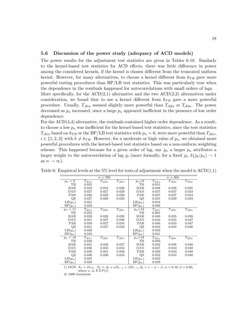
The power results for the adjustment test statistics are given in Tables 6-10. Similarlyto the kernel-based test statistics for ACD effects, there was little difference in poweramong the considered kernels, if the kernel is chosen different from the truncated uniformkernel. However, for many alternatives, to choose a kernel different from kTR gave morepowerful testing procedures than BP/LB test statistics. This was particularly true whenthe dependence in the residuals happened for autocorrelations with small orders of lags.More specifically, for the ACD(2,1) alternative and the two ACD(2,2) alternatives underconsideration, we found that to use a kernel different from kTR gave a more powerfulprocedure. Usually, TA1n seemed slightly more powerful than TA2n or TA3n. The powerdecreased as pn increased, since a large pn appeared inefficient in the presence of low orderdependence.For the ACD(4,4) alternative, the residuals contained higher order dependence. As a result,to choose a low pn was inefficient for the kernel-based test statistics, since the test statisticsTA1n based on kTR or the BP/LB test statistics with pn = 6, were more powerful than TAin,i ∈ 1, 2, 3 with k = kTR. However, for a moderate or high value of pn, we obtained morepowerful procedures with the kernel-based test statistics based on a non-uniform weightingscheme. This happened because for a given order of lag, say j0, a larger pn attributes alarger weight to the autocorrelation of lag j0 (more formally, for a fixed j0, k(j0/pn) → 1as n → ∞).

Table 6: Empirical levels at the 5% level for tests of adjustment when the model is ACD(1,1)n = 256 n = 384

pn = 6 TA1n TA2n TA3n pn=6 TA1n TA2n TA3nTR 0.035 TR 0.051

BAR 0.022 0.024 0.026 BAR 0.038 0.038 0.035DAN 0.027 0.027 0.029 DAN 0.037 0.037 0.033PAR 0.026 0.028 0.030 PAR 0.037 0.037 0.034QS 0.027 0.029 0.029 QS 0.037 0.039 0.033

LB(pn) 0.021 LB(pn) 0.034BP(pn) 0.023 BP(pn) 0.036pn = 11 TA1n TA2n TA3n pn=12 TA1n TA2n TA3n

TR 0.052 TR 0.061BAR 0.028 0.028 0.028 BAR 0.040 0.035 0.038DAN 0.031 0.027 0.030 DAN 0.044 0.045 0.047PAR 0.030 0.027 0.034 PAR 0.046 0.043 0.047QS 0.031 0.027 0.032 QS 0.044 0.044 0.046

LB(pn) 0.029 LB(pn) 0.033BP(pn) 0.033 BP(pn) 0.041pn = 16 TA1n TA2n TA3n pn=18 TA1n TA2n TA3n



1) DGP: Xt = Dtεt, Dt = β0 + αXt−1 + βDt−1, β0 = 1 − α− β, α = 0.18, β = 0.80,where εt is EXP (1)

2) 1000 iterations

19

Table 7: Level-adjusted powers against ACD(2,1) at 5% level for tests of adjustment whenthe model is ACD(1,1)

n = 256 n = 384pn = 6 TA1n TA2n TA3n pn = 6 TA1n TA2n TA3n


LB(pn) 0.470 LB(pn) 0.628BP(pn) 0.470 BP(pn) 0.628pn = 11 TA1n TA2n TA3n pn = 12 TA1n TA2n TA3n





1) DGP: Xt = Dtεt, εt ∼ EXP (1), Dt = β0 + α1Xt−1 + α2Xt−2 + β1Dt−1,β0 = 1 − α1 − α2 − β1, α1 = 0.3, α2 = 0.4, β1 = 0.1

2) 500 iterations

Table 8: Level-adjusted powers against ACD(2,2)a at 5% level for tests of adjustment whenthe model is ACD(1,1)








1) DGP: Xt = Dtεt, εt ∼ EXP (1), Dt = β0 + α1Xt−1 + α2Xt−2 + β1Dt−1 + β2Dt−2,β0 = 1 − α1 − α2 − β1 − β2, α1 = 0.1, α2 = 0.3, β1 = 0.1, β2 = 0.3

2) 500 iterations

20

Table 9: Level-adjusted powers against ACD(2,2)b at 5% level for tests of adjustment whenthe model is ACD(1,1)








1) DGP: Xt = Dtεt, εt ∼ EXP (1), Dt = β0 + α1Xt−1 + α2Xt−2 + β1Dt−1 + β2Dt−2,β0 = 1 − α1 − α2 − β1 − β2, α1 = 0.2, α2 = 0.4, β1 = 0, β2 = 0.2

2) 500 iterations

Table 10: Level-adjusted powers against ACD(4,4) at 5% level for tests of adjustment whenthe model is ACD(1,1)








1) DGP: Xt = Dtεt, Dt = β0 +∑4

i=1 αiXt−i +∑4

i=1 βiDt−i, β0 = 1 − ∑4i=1(αi + βi),

α1 = α2 = α3 = β1 = β2 = β3 = 0, α4 = 0.2, β4 = 0.1, εt ∼ EXP (1)2) 500 iterations

21

6 Application with IBM Data

In this section we analyze the IBM transaction data taken from the TORQ (Trades, Orders,Reports, and Quotes) data set compiled by Hasbrouck (1991) and the New York Stock Ex-change (NYSE). The same database was used by Engle and Russell (1998) to implementthe ACD models. The NYSE is the world’s largest equities market with a $12.3 trillionglobal market capitalization in September 30, 2002. The market combines the features ofa price-driven market (presence of a market maker) with those of an order-driven market(existence of an order book), which makes it an explicitly hybrid mechanism. Specifically,each stock is allocated to a single market maker, named specialist, who must ensure anorderly market in that stock and therefore commit his own capital while taking positionagainst the trend of the market until stability is achieved. However, the specialist must alsomonitor the order book for the stock in which limit orders are transmitted electronicallyor via a floor trader (see Hasbrouck et al. (1993) for a description of the operations of theNYSE). The NYSE opens with a call auction implemented to find the opening price andthen trading occurs continuously from 9h30 to 16h. In our study, we will focus principallyon the trade durations (i.e. time intervals between successive trades). Trade durationsare indicators for the trading activity and they are receiving an increasing attention in thefinancial literature on market microstructure. For example, several studies were concernedwith how the timing of trades affects market behavior and the formation of prices. Theso-called asymmetric information models, developed in more recent research on marketmicrostructure assume that trades convey information. For example, if some traders arebetter informed than others, it seems plausible in such circumstances that their tradescould reveal some information. Glosten and Milgrom (1985), Easley and O’Hara (1992),Diamond and Verrecchia (1987) and Admati and Pfleiderer (1988), among others, empha-sized this notion of time as signal and the role of intertrade durations for explaining howthe information is processed in financial markets. O’Hara (1995) provides an excellentreview of the market microstructure theory.

In our database, the sample period runs over three months, from November 1, 1990through January 31, 1991. The initial sample contains 60328 transactions for a total of 63trading days. For each transaction, the information recorded contains the calendar date,a time stamp measured in seconds after midnight at which the transaction took place,the volume of shares traded, the bid and ask price at the time of trade and finally thetransaction price. Following Engle and Russell (1998) and Engle (2000), the interdailydurations (i.e. the overnight durations) as well as transactions occurring outside regulartrading hours were removed. Moreover, transactions on Thanksgiving Friday and the daybefore Christmas and New Year were deleted since these days were characterized by a slowlyactivity compared to the rest of the sample. Trades occurring simultaneously (thus leadingto zero durations) were also discarded. This uses the microstructure argument that zerodurations correspond to ’split-transactions’ (i.e. one big order which is matched againstseveral smaller opposite orders). Veredas, Rodriguez-Poo, and Espasa (2002) proposeanother way for dealing with zero durations but for simplicity, we proceeded as in Engle andRussell (1998) and Engle (2000). The sample thus reduced to 52146 observations. Table 11

22

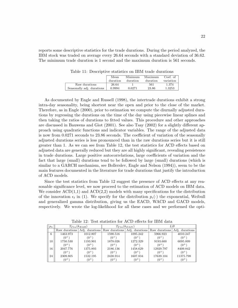
reports some descriptive statistics for the trade durations. During the period analyzed, theIBM stock was traded on average every 26.64 seconds with a standard deviation of 36.62.The minimum trade duration is 1 second and the maximum duration is 561 seconds.

Table 11: Descriptive statistics on IBM trade durationsMean Minimum Maximum Coef. of

duration duration duration variationRaw durations 26.64 1 561 1.374

Seasonally adj. durations 0.9994 0.0271 23.86 1.3253

As documented by Engle and Russell (1998), the intertrade durations exhibit a strongintra-day seasonality, being shortest near the open and prior to the close of the market.Therefore, as in Engle (2000), prior to estimation we compute the diurnally adjusted dura-tions by regressing the durations on the time of the day using piecewise linear splines andthen taking the ratios of durations to fitted values. This procedure and other approachesare discussed in Bauwens and Giot (2001). See also Tsay (2002) for a slightly different ap-proach using quadratic functions and indicator variables. The range of the adjusted datais now from 0.0271 seconds to 23.86 seconds. The coefficient of variation of the seasonallyadjusted durations series is less pronounced than in the raw durations series but it is stillgreater than 1. As we can see from Table 12, the test statistics for ACD effects based onadjusted data are generally reduced but they are all highly significant, revealing persistencein trade durations. Large positive autocorrelations, large coefficients of variation and thefact that large (small) durations tend to be followed by large (small) durations (which issimilar to a GARCH mechanism, see Bollerslev, Engle and Nelson (1994)), seem to be themain features documented in the literature for trade durations that justify the introductionof ACD models.

Since the test statistics from Table 12 suggest the presence of ACD effects at any rea-sonable significance level, we now proceed to the estimation of ACD models on IBM data.We consider ACD(1,1) and ACD(2,2) models with many specifications for the distributionof the innovation εt in (1). We specify for the distribution pε(·) the exponential, Weibulland generalized gamma distribution, giving us the EACD, WACD and GACD models,respectively. We wrote the log-likelihood for all these cases and we performed the opti-

Table 12: Test statistics for ACD effects for IBM datapn TE1n(kBAR) TE1n(kDAN ) LB

Raw durations Adj. durations Raw durations Adj. durations Raw durations Adj. durations6 1463.973 1012.807 1590.516 1095.242 5966.923 4010.247

(0+) (0+) (0+) (0+) (0+) (0+)10 1750.530 1193.901 1878.026 1272.329 9193.600 6095.899

(0+) (0+) (0+) (0+) (0+) (0+)16 2047.776 1375.893 2186.136 1458.629 12929.797 8409.842

(0+) (0+) (0+) (0+) (0+) (0+)24 2309.805 1532.195 2438.914 1607.834 17639.104 11375.798

(0+) (0+) (0+) (0+) (0+) (0+)

23

mization via the Nelder-Mead simplex method, using MATLAB software. We applied ourtest procedures TA1n with the Daniell (kDAN ), Bartlett (kBAR) and truncated uniform(kTR) kernels. Tables 13, 14 and 15 report the test statistics with the corresponding p-values. The ACD(1,1) seemed inappropriate since all the p-values are highly significant.The ACD(2,2) provided an improvement over the ACD(1,1) model, since the p-values ofthe test statistics are generally higher. Since the truncated uniform kernel attributes equalweighting for each considered lag, it seems plausible that high residual autocorrelations arestill present in the EACD(2,2) and WACD(2,2) models, since for pn = 16 the test statisticTA1n(kTR) rejects the null hypothesis of adequacy, and for pn = 24 the same can be saidfor TA1n(kBAR) and TA1n(kDAN ). It seemed that the GACD(2,2) gave the best fit for thesedata, since the p-values of the test statistics TA1n(kBAR) and TA1n(kDAN ) are larger than5% or very close to it. The test statistic TA1n(kTR) seems to suggest that some large au-tocorrelations are still present, since TA1n(kTR) with pn = 16 is still significant. However,with more that 50000 observations, that test statistic is very close to the 1% significancelevel. Furthermore, the test statistics with Bartlett and Daniell kernels, which have beenshown to be more powerful than TA1n(kTR) in many situations (see the simulations of theSection 5), seem to indicate the adequacy of the GACD(2,2) model. Overall, we concludethat the GACD(2,2) provides a rather satisfactory adjustment over the GACD(1,1) modelsince with this sample size, the test statistics from Table 15 do not clearly indicate aninadequate model.

Table 13: Test statistics for adjustment of EACD(1,1) and EACD(2,2) models for IBMdata

EACD(1,1) EACD(2,2)pn TA1n(kTR) TA1n(kBAR) TA1n(kDAN ) TA1n(kTR) TA1n(kBAR) TA1n(kDAN )6 4.094 6.610 6.447 2.587 0.341 0.380

(0+) (0+) (0+) (0.005) (0.366) (0.352)10 2.756 5.577 5.484 1.516 1.197 1.566

(0.003) (0+) (0+) (0.065) (0.116) (0.059)16 6.303 4.780 4.305 2.748 1.606 1.756

(0+) (0+) (0+) (0.003) (0.054) (0.039)24 6.041 5.213 5.218 1.432 2.012 2.219

(0+) (0+) (0+) (0.076) (0.022) (0.013)

Table 14: Test statistics for adjustment of WACD(1,1) and WACD(2,2) models for IBMdata

WACD(1,1) WACD(2,2)pn TA1n(kTR) TA1n(kBAR) TA1n(kDAN ) TA1n(kTR) TA1n(kBAR) TA1n(kDAN )6 3.970 6.282 6.127 2.716 0.343 0.394

(0+) (0+) (0+) (0.003) (0.366) (0.347)10 2.679 5.320 5.250 1.648 1.257 1.651

(0.004) (0+) (0+) (0.050) (0.104) (0.049)16 6.243 4.593 4.148 2.970 1.714 1.881

(0+) (0+) (0+) (0.001) (0.043) (0.030)24 5.929 5.070 5.097 1.615 2.166 2.393

(0+) (0+) (0+) (0.053) (0.015) (0.008)

24

Table 15: Test statistics for adjustment of GACD(1,1) and GACD(2,2) models for IBMdata

GACD(1,1) GACD(2,2)pn TA1n(kTR) TA1n(kBAR) TA1n(kDAN ) TA1n(kTR) TA1n(kBAR) TA1n(kDAN )6 3.871 6.507 6.275 2.157 0.719 0.692

(0+) (0+) (0+) (0.015) (0.236) (0.244)10 2.481 5.424 5.170 1.147 1.201 1.432

(0.006) (0+) (0+) (0.126) (0.115) (0.076)16 4.978 4.508 3.900 2.384 1.396 1.431

(0+) (0+) (0+) (0.008) (0.081) (0.076)24 4.002 4.549 4.310 1.133 1.708 1.834

(0+) (0+) (0+) (0.128) (0.044) (0.033)

Conclusion

In this paper, we have proposed two classes of test statistics for duration clustering and anew class of diagnostic test statistics for ACD models, using a spectral approach. Whentesting for ACD effects, the test statistics in the first class are based on a distance measureand a kernel-based spectral density estimator of the raw durations. On the other side,the test statistics in the second class exploit the one-sided nature of duration clustering.Asymptotic arguments suggest that the test statistics in the first class should be morepowerful asymptotically, but to exploit the one-sided nature of the alternative hypothesismay be particularly powerful in small samples. A small sample size could occur whenthe market participants are interested in volume durations, among others. When testingfor adequacy, we proposed a class of test statistics using a kernel-based spectral densityestimator of the estimated standardized duration residuals. We established the asymptoticdistributions of the test statistics for duration clustering and for the adequacy of ACDmodels, which are normal under their respective null hypothesis. We also discussed whenthe tests in a given class are asymptotically equivalent under the null hypothesis.

Empirical experiments have been conducted to evaluate the proposed procedures. Wefound that all the proposed test statistics have reasonable levels. Typically, the weightingscheme of the kernel-based test statistics attributes more (less) weight to low (high) ordersof lags. We found that in many circumstances such weighting contributes to powerful pro-cedures. In many situations, the proposed test statistics were more powerful than BP/LBtest statistics. When ACD effects were particularly persistent, the test statistics in thesecond class were usually more powerful. Similarly, when testing for the adequacy of ACDmodels, the proposed test statistics had reasonable levels. Interestingly, our generalized BPtest statistic appeared to have better empirical levels than BP/LB test statistics, at leastin our experiments. Concerning the power, usually a kernel different from the truncateduniform kernel lead to more powerful procedures, since the kernel-based test statistics (withk = kTR), were more powerful than BP/LB test statistics, for the chosen models.

We illustrated our test procedures on the IBM dataset considered in Engle and Russell(1998). We found that the GACD(2,2) provided a rather satisfactory adjustment, since

25

with a sample size of more that 50000 observations, the test statistics based on the trun-cated uniform, Bartlett and Daniell kernels, did not clearly indicate an inadequate model.

References

Admati, A.R. and Pfleiderer, P. (1988), “A theory of intraday patterns: volume and pricevariability”, The Review of Financial Studies, 1, 3-40.

Bauwens, L. and Giot, P. (2000a), “The Logarithmic ACD model: An Application tothe Bid-Ask Quote Process of Three NYSE stocks”, CORE discussion paper, 9789,Universite Catholique de Louvain.

Bauwens, L. and Giot, P. (2000b), “Asymmetric ACD Models: Introducing Price Informa-tion in ACD models”, CORE discussion paper, 9844, Universite Catholique de Louvain.

Bauwens, L. and Giot, P. (2001), Econometric modelling of stock market intraday activity,Advances Studies in Theoretical and Applied Econometrics, Kluwer Academic Publish-ers: Boston.

Bollerslev, T., Engle, R. F. and Nelson, D. B. (1994), “ARCH models” in Handbook ofEconometrics, vol. IV, eds R.F. Engle and D.L. McFadden, Amsterdam, Elsevier Sci-ence, 2959–3038.

Box, G.E.P. and Pierce, D. (1970), “Distribution of Residual Autocorrelations in Autore-gressive Integrated Moving Average Time Series Models”, Journal of the AmericanStatistical Association, 65, 1509-1526.

Diamond, D.W. and Verrecchia, R.E. (1987), “Constraints on short-selling and asset priceadjustments to private information”, Journal of Financial Economics, 18, 277-311.

Drost, F.C. and Werker, B.J.M. (2000), “Efficient Estimation in Semiparametric TimeSeries: the ACD model”, Working paper, Tilburg University.

Easley, D. and O’Hara, M. (1992), “Time and the Process of Security Price Adjustment”,The Journal of Finance, 19, 69-90.

Engle, R.F. (2000), “The Econometrics of Ultra-High Frequency Data”, Econometrica, 68,1-22.

Engle, R.F. and Russell, J.R. (1997), “Forecasting the Frequency of Changes in QuotedForeign Exchange Prices with the Autoregressive Conditional Duration Model”, Journalof Empirical Finance, 4, 187-212.

Engle, R.F. and Russell, J.R. (1998), “Autoregressive Conditional Duration: A New Modelfor Irregularly Spaced Transaction Data’, Econometrica, 66, 1127-1162.

Engle, R.F. and Russell, J.R. (2002), “Analysis of high frequency data”, Manuscript.Fernandes, M. and Graming, J. (2000), “Non-parametric Specification Tests for Conditional

Duration Models”, Working paper, European University Institute and University ofFrankfurt.

26

Ghysels, E. and Jasiak, J. (1998a), “Long-term Dependence in Trading”, Working paper,Dept. of Economics, Penn State University and York University.

Ghysels, E. and Jasiak, J. (1998b), “GARCH for Irregularly Spaced Financial Data: TheACD-GARCH Model”, Studies in Nonlinear Economics and Econometrics, 2, 133-149.

Glosten, L. and Milgrom, P. (1985), “Bid, ask and transaction prices in a specialist marketwith heterogeneously informed traders”, Journal of Financial Economics, 14, 71-100.

Graming, J. and Maurer, K.-O. (2000), “Non-monotonic hazard functions and the autore-gressive conditional duration model”, Econometrics Journal, 3, 16-38.

Hasbrouck, J. (1991), “Measuring the Information Content of Stock Trades”, The Journalof Finance, 66, 1, 179-207.

Hasbrouck, J., Sofianos, G. and Sosebee, D. (1993), “New York Stock Exchange systemsand trading procedures”, Working paper 93-01, New York Stock Exchange.

Hong, Y. (1996), “Consistent testing for serial correlation of unknown form”, Econometrica,64, 837–864.

Hong, Y. (1997), “One-sided testing for conditional heteroskedasticity in time series mod-els”, Journal of Time Series Analysis, 18, 253–277.

Hong, Y. and Shehadeh, R. D. (1999), “A new test for ARCH effects and its finite-sampleperformance”, Journal of Business and Economic Statistics, 17, 91–108.

Jasiak, J. (1999), “Persistence in Intertrade Durations”, Working paper, Department ofEconomics, York University, Toronto.

Lee, J.H.H. and King, M.L. (1993), “A Locally Most Mean Powerful Based Score Testfor ARCH and GARCH Regression Disturbances”, Journal of Business and EconomicStatistics, 11, 17-27. (Correction 1994, 12, p. 139).

Ljung, G.M. and Box, G.E.P. (1978), “On a Measure of Lack of Fit in Time Series Models”,Biometrika, 65, 297-303.

Nelson, D. and Cao, C.Q. (1992), “Inequality Constraints in the Univariate GARCHModel”, Journal of Business and Economic Statistics, 10, 229-235.

O’Hara, M. (1995), Market microstructure theory, Basil Blackwell: Oxford, England.Priestley, M. B. (1981), Univariate Series, Vol. 1 of Spectral Analysis and Time Series,

Academic Press:New-York.Tsay, R. S. (2002), Analysis of financial time series, Wiley: New York.Veredas, D., Rodriguez-Poo, J. and Espasa, A. (2001), “On the (intradaily) seasonality

and dynamics of a financial point process: a semiparametric approach”, Working paper2001-19, INSEE, Paris.

Zhang, M. Y., Russell, J. R. and Tsay, R. S. (2001), “A nonlinear autoregressive conditionalduration model with applications to financial transaction data”, Journal of Economet-rics, 104, 179-207.

Les Cahiers du CREF ISSN: 1707-410XLes Cahiers du CREF CREF 03-05 Résumé Les modèles de durée...

Documents

Transcript of Les Cahiers du CREF ISSN: 1707-410XLes Cahiers du CREF CREF 03-05 Résumé Les modèles de durée...