Leo Ducrot Master of engineering, Institut Catholique d ...

Investigation of potential added value of DDMRP in planning under uncertainty at finite capacity

by

Leo Ducrot Master of engineering, Institut Catholique d'Arts et Métiers, 2009

Master of Industrial Management, K.U. Leuven, 2010

and Ehtesham Ahmed

Bachelor of Business Administration, Institute of Business Administration, 2011 Master of Business Administration, Institute of Business Administration, 2015

SUBMITTED TO THE PROGRAM IN SUPPLY CHAIN MANAGEMENT

IN PARTIAL FULFILLMENT OF THE REQUIREMENTS FOR THE DEGREE OF MASTER OF APPLIED SCIENCE IN SUPPLY CHAIN MANAGEMENT

AT THE MASSACHUSETTS INSTITUTE OF TECHNOLOGY

JUNE 2019

© 2019 Leo Ducrot and Ehtesham Ahmed. All rights reserved. The authors hereby grant to MIT permission to reproduce and to distribute publicly paper and electronic

copies of this capstone document in whole or in part in any medium now known or hereafter created.

Signature of Author: ____________________________________________________________________ Leo Ducrot

Department of Supply Chain Management May 10, 2019

Signature of Author: ____________________________________________________________________

Ehtesham Ahmed Department of Supply Chain Management

May 10, 2019 Certified by: __________________________________________________________________________

Dr. Sergio Alex Caballero Research Scientist Capstone Advisor

Certified by: __________________________________________________________________________ Dr. Tugba Efendigil Research Scientist

Capstone Co-Advisor

Accepted by: __________________________________________________________________________ Dr. Yossi Sheffi

Director, Center for Transportation and Logistics Elisha Gray II Professor of Engineering Systems Professor, Civil and Environmental Engineering

2

Investigation of Potential Added Value of DDMRP in Planning Under Uncertainty at Finite Capacity

by

Leo Ducrot

and

Ehtesham Ahmed

Submitted to the Program in Supply Chain Management on May 10, 2019 in Partial Fulfillment of the

Requirements for the Degree of Master of Applied Science in Supply Chain Management

ABSTRACT

The Demand Driven Material Requirement Planning (DDMRP) was introduced in 2011 to improve the performance of supply chain planning. The Demand Driven Institute (DDI) reports that DDMRP reduces the inventory levels by 31% (median) while improving the service level by 13% (median) and reducing the customer order lead time. Such results can have a significant impact on the financial performance of a company and provide a competitive advantage. In this project, we investigate how DDMRP operates in a capacity constrained environment. Qualitative and quantitative techniques were used to collect data about the real-life implementations of DDMRP for different size companies operating in various industries. Afterward, a simulation analysis was carried out to compare the algorithms of DDMRP and Advanced Planning System (APS). Our results show that DDMRP outperforms heuristics-based planning and provides similar results as a solver-based planning. Our survey confirmed the order of magnitude of the improvements claimed by the DDI in terms of service level, inventory level, and customer order lead time. In addition, we learned that implementing DDMRP forces the company to develop extended supply chain training programs across the company. These programs combined with the focus on product flow from the demand driven approach help the companies to streamline their operations. Streamlined operations is essential to maintain the service level high and the inventory low over time. This research proves that DDMRP can perform well in planning at finite capacity under uncertainty. DDMRP can reduce the working capital and offer a competitive advantage, which gives DDMRP the potential to be a game-changer in supply chain planning.

Capstone Advisor: Sergio Alex Caballero Title: Research Scientist

Capstone Co-Advisor: Tugba Efendigil Title: Research Scientist

3

ACKNOWLEDGMENTS

First and foremost, we would like to thank our advisors Dr. Sergio Caballero and Dr. Tugba Efendigil for their help, their guidance and their patience throughout the project.

We are grateful to Carol Ptak, partners at Demand Driven Institute, Steve Honkomp, Sr. Product Supply Business Intelligence Analyst at Procter&Gamble and Dirk Van Ginderachter, associate director at OM Partners, sponsors of this project for their time, their availability and their precious help. Their feedbacks were very valuable and helpful.

We would like to thank the class SCM 2019 for the incredible level of collaboration and trust, and for the spectacular time spent together.

I also want to thank my wife Anna, for her support and for making it through this long-distance journey. I would like to thank Marion Konnerth, Kristof Van Cauwenberghe, Sunitha Ray, Elissar Samaha and Neysan Kamranpour for their direct or indirect help in the project.

- Leo

I would like to acknowledge my wife Javaria and all the other people who made it possible for me to go through this amazing journey at MIT.

I would also like to appreciate my co-author Leo Ducrot for answering all my questions, on DDMRP and APS, throughout the nine months and his hard-work, dedication, and perseverance on this project.

- Ehtesham.

4

Contents 1. Introduction .................................................................................................................................... 6

1.1 Description of the problem ............................................................................................................ 7

1.2 Objective and Scope....................................................................................................................... 7

2. Literature Review ............................................................................................................................ 9

2.1 MRP ............................................................................................................................................... 9

2.2 APS .............................................................................................................................................. 10

2.3 DDMRP ........................................................................................................................................ 12

2.4 DDMRP vs MRP ............................................................................................................................ 14

3. Methodology ................................................................................................................................. 17

3.1 Qualitative and Quantitative Research ......................................................................................... 18

3.1.1. Interviews ....................................................................................................................... 18

3.1.2. Survey ............................................................................................................................ 19

3.2 Simulation Analysis................................................................................................................. 19

4. The Simulation .................................................................................................................................. 21

4.1 The Simulation Workflow ............................................................................................................. 21

4.2 Description of the assumptions and the planning algorithms ....................................................... 23

4.3 Description of the company ......................................................................................................... 24

5. Results ........................................................................................................................................... 26

5.1 Qualitative and Quantitative Research Results ............................................................................. 26

5.2 Simulation Analysis Results .......................................................................................................... 33

5.2.1 Scenario 1: Low forecast accuracy and low capacity constraints ............................................ 33

5.2.2 Scenario 2: Low forecast accuracy and high capacity constraints ........................................... 35

5.2.3 Scenario 3: Variable operations and low capacity constraints ................................................ 37

5.2.4 Scenario 4: Variable operations and high capacity constraints ............................................... 38

6. Discussion ......................................................................................................................................... 40

7. Conclusion ......................................................................................................................................... 44

References ............................................................................................................................................ 45

Appendix A – Interview Questions ......................................................................................................... 48

Appendix B: Survey Questions ............................................................................................................... 49

Appendix C – Simulation data and data generation ................................................................................ 52

5

List of Tables

Table 1: Supply chain circumstances, 1965 versus today ........................................................................ 12 Table 2: Scenarios .................................................................................................................................. 20 Table 3: Repartition of companies per industry ...................................................................................... 26 Table 4: Average service level improvement per industry ...................................................................... 27 Table 5: Impact Of DDMRP On Operations For All Companies ................................................................ 29 Table 6: Impact of DDMRP on operations per legacy system .................................................................. 29 Table 7: Impact of DDMRP on operations per maturity level .................................................................. 30 Table 8: Effectiveness of DDMRP ........................................................................................................... 32 Table 9: Overview of the simulation results ........................................................................................... 33 Table 10: Scenario 1 results ................................................................................................................... 34 Table 11: Scenario 2 results ................................................................................................................... 36 Table 12: Scenario 3 results ................................................................................................................... 37 Table 13: Scenario 4 results ................................................................................................................... 39

List of Figures

Figure 1: Methodology for investigating the potential added value of DDMRP in planning under uncertainty at finite capacity ................................................................................................................. 17 Figure 2: Scenario Flowchart ................................................................................................................. 21 Figure 3: Inventory turns before and after DDMRP implementation ...................................................... 27 Figure 4: Improvements in the operations with DDMRP ......................................................................... 28 Figure 5: Problems with legacy systems ................................................................................................. 30 Figure 6: Service level vs inventory turns Scenario 1 .............................................................................. 35 Figure 7: Service levels vs inventory turns scenario 2 ............................................................................. 36 Figure 8: Service Level vs Inventory Turns Scenario 3 ............................................................................. 38 Figure 9: Service Level vs Inventory Turns Scenario 4 ............................................................................. 39

6

1. Introduction

In 1964, the first Materials Requirement Planning (MRP) was successfully implemented in Black &

Decker. MRP was developed by Joseph Orlicky (Orlicky, 1975). Oliver Wight, in 1983, extended MRP

further, which became MRP II or Manufacturing Resource Planning (Hopp & Spearman, 2004). The

purpose of MRP and MRP II was to couple the production and the sourcing activities to the final

demand.

In the 1990s, Advanced Planning and Scheduling (APS) systems were introduced. APS systems use

algorithms and, mathematical optimization to plan the demand, production and procurement.

The supply chains of today are more complex than they were in the 1960s. The number of products has

increased, and so has the transportation and procurement lead times. This has introduced more

variability and uncertainty in the supply chains.

In 2011 a new planning methodology called Demand Driven MRP (DDMRP) was introduced in response

to the new dynamics of supply chain complexity. DDMRP is a multi-echelon supply chain planning

approach that combines the best of lean, MRP, six-sigma and the theory of constraints. It relies on the

idea that ROI comes from emphasizing the flow of product to the market rather than mere unit cost

reductions. DDMRP proposes an intuitive way to manage flows of products and relevant information by

strategically positioning decoupling points and managing those with clear inventory policies. DDMRP has

a particular focus on managing variability and planning and execution priorities.

DDMRP replaces the Master Production Schedule (MPS) by a day-to-day process to generate supply

orders. Removing the projected stock could prove difficult to handle planning complexity such as strong

capacity constraints, alternative BOMs, complex machinery routes, or shifting bottlenecks. The Demand

7

Driven Institute (DDI) states that it is possible to handle these situations with the well positioned and

managed buffers, and with feedback loops to adjust the model when it is required.

This project was sponsored by the Demand Driven Institute, OM Partners and a CPG company. These

sponsorships created a balanced project team that helped make the project successful.

1.1 Description of the problem

DDMRP has been presented as an effective tool for improving supply chain planning in conditions of

demand or operations uncertainty and complexity. The Demand Driven Institute (DDI) has published

results of DDMRP implementations that show an increase in service levels by 13%, reduction in

inventory by 31%, and a decrease in lead times by 22% (Camelot, 2019). However, these are median

results and different industries can have different results.

These results may appear “too good to be true.” Furthermore, DDI does not provide insights on which

production planning methodology was used by these companies before their DDMRP implementations.

The initial results displayed by the DDI can significantly improve the financial performance of a company.

The improvement in service level and the contraction of customer order lead time can provide a

competitive advantage. However, further analysis is required to understand what conditions are

required to achieve this level of improvement.

1.2 Objective and Scope

This project aims at better understanding what results can be expected from a DDMRP implementation.

We will investigate inventory saving, service level improvements and customer order lead time

8

contraction. The objective is to provide practitioners with valuable information on the added value of

DDMRP in complex planning situations. We focus on finite capacity constraint and alternative sourcing

because these constraints are often encountered in manufacturing companies.

This paper will try to answer the question “What are the potential added values of DDMRP in planning

under uncertainty at finite capacity?”

To answer that question, we apply both quantitative and qualitative analysis. In the quantitative

segment of our research, we conducted a simulation using DDMRP and different planning algorithms

available in an APS to evaluate and compare their impact on service level, inventory level, and inventory

turns for a Consumer-Packaged Goods (CPG) company. In the qualitative part of our research, we

surveyed companies that are using DDMRP to learn what benefits they have realized and what

drawbacks they have encountered. The survey’s findings were compared to the simulation results in

order to provide an assessment of the performances of DDMRP in constrained planning situations.

9

2. Literature Review

In this section, we will review the literature on the MRP, APS, and DDMRP. This section presents the

drawbacks of MRP and APS found in the literature.

Since DDMRP was first published in 2011, not a lot of academic material has been published on the

topic. There are books from DDI that provide an understanding of DDMRP and two academic articles

that provide results comparing DDMRP with MRP. However, we have not found any comparison

between DDMRP and APS in academic research. Many companies have shifted from MRP to APS since it

provides better results than MRP. In truth, APS has also been able to address MRP’s shortcomings and

provides a better result than MRP (Moscoso, Fransoo, & Fischer, 2010).

2.1 MRP

According to Ptak & Smith (2011), MRP has existed in some form in manufacturing industries but

improvements in computer-aided data processing have allowed comprehensive and robust systems to

be created. APICS defines MRP as “…set of techniques that uses bill of materials data, inventory data

and the master production schedule to calculate requirements for materials.” (APICS, 2015)

The objective of MRP systems is to meet the customer requirements or forecasts across the company.

These requirements are converted into net requirements. The output of the net requirements are the

production orders and purchase orders.

Many authors classify planned instability and nervousness as a major limitation in MRP systems (Ho,

Law, & R., 1995; Heisig, 2002; Blackburn, Kropp, & Millen,1986). Carlson, Jucker, and Kropp (1979) state

that nervousness occurs because of frequent changes in production schedules. Minifie and Davis (1990)

define nervousness as production schedule changes that take place in upper levels that are not due to

10

changes in the independent requirements. Changes in the upper levels are introduced by changes in the

production plans of the lower levels.

The founders of DDMRP, Ptak and Smith (2011), have emphasized that for an MRP system to run, actual

customer requirements is required. However, due to lead time, it is impossible to only base the plan on

actual demand. This requires the use of forecasted demand. Burbridge (1980) states that it is impossible

to make accurate forecasts for long periods. Therefore, incorrect forecasts are fed into MRP systems in

place of actual demand causing nervousness.

Another challenge is the use of traditional inventory control systems with MRP. This increases

inventories, decreases service levels (Tempelmier, 2001) and results are long wait time for customers.

Among the proposed solutions to handle nervousness, the most commonly used are safety stock or

safety lead-time or safety capacity. Ho et al. (1995), Whybark and Williams (1976), and New (1975)

maintain that safety stock is the preferred technique to control quantity uncertainty and is the primary

protection against overall uncertainty in the system. However, a study showed that safety stock could

also, in certain circumstances, amplify the variability and the instability in the system (Sridharan and

LaForge, 1990).

2.2 APS

APICS defined APS as ‘…any computer program that uses advanced mathematical algorithms or logic to

perform optimization or simulation on finite capacity scheduling, sourcing, capital planning, resource

planning, forecasting, demand management, and others. These techniques simultaneously consider a

range of constraints and business rules to provide real-time planning and scheduling, decision support,

available-to-promise, and capable-to-promise capabilities. APS often generates and evaluates multiple

scenarios…” (APICS, 2015)

11

As there are only broad definitions for APS systems, it is important to specify which algorithm is used

when an APS system is involved in a comparison. According to Gruat-La-Forme, Botta-Genoulaz,

Campagne, and Millet (2005), the key success factors of APS are real-time overview, good decision

support systems, and real-time scheduling. While taking into account constraints, capacity and changes.

Hvolby and Steger-Jensen (2010) have reported that early adopters of APS systems achieved 300%

return on investment.

In the literature, we find that APS provides better results than MRP. In a study conducted by Moscoso,

Fransoo, and Fischer (2010), the APS implementation had a positive result. Backlogs were reduced by

84% (in three months) and 97% service levels were achieved. However, they also found that average

production lead time increased by 15%. Hvolby and Steger-Jensen (2010) in their study found that

delivery accuracy went up from 79% to 99% after implementing an APS system. Overall lead-time was

reduced from seven days to zero and use of planning resources reduced by 30%. Gruat-La-Forme, Botta-

Genoulaz, Campagne, and Millet (2005) have identified that an APS system leads to a reduction in

inventory, reduction in safety stock, increase in service levels and reduction in overall costs.

Genin, Thomas, & Lamouri (2007) used a simulation to argue that APS systems are more robust if

planning time fences are managed properly. According to Moscoso et al. (2010), in APS there is no

planning instability. The observed instability is due to organizational structure and human decision

factors.

However, implementing an APS system is challenging, and according to Funk (2001) over 80% of all

implementations were classified as failures since the results failed to achieve the initially projected

business economic gains.

12

2.3 DDMRP

Smith and Smith (2013) have observed that complexity and volatility faced by supply chains have greatly

increased since the seventies and refer to it as the ‘New Normal’.

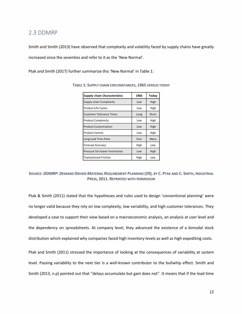
Ptak and Smith (2017) further summarize this ‘New Normal’ in Table 1:

TABLE 1: SUPPLY CHAIN CIRCUMSTANCES, 1965 VERSUS TODAY

SOURCE: DDMRP: DEMAND DRIVEN MATERIAL REQUIREMENT PLANNING (29), BY C. PTAK AND C. SMITH, INDUSTRIAL PRESS, 2011. REPRINTED WITH PERMISSION

Ptak & Smith (2011) stated that the hypotheses and rules used to design ‘conventional planning’ were

no longer valid because they rely on low complexity, low variability, and high customer tolerances. They

developed a case to support their view based on a macroeconomic analysis, an analysis at user level and

the dependency on spreadsheets. At company level, they advanced the existence of a bimodal stock

distribution which explained why companies faced high inventory levels as well as high expediting costs.

Ptak and Smith (2011) stressed the importance of looking at the consequences of variability at system

level. Passing variability to the next tier is a well-known contributor to the bullwhip effect. Smith and

Smith (2013, n.p) pointed out that “delays accumulate but gain does not”. It means that if the lead time

Supply chain Characteristics 1965 Today

Supply chain Complexity Low High

Product Life Cycles Low High

Customer Tolerance Times Long Short

Product Complexity Low High

Product Customization Low High

Product Variety Low High

Long Lead Time Parts Few Many

Forecast Accuracy High Low

Pressure for leaner Inventories Low High

Transactional Friction High Low

13

to replenish (procurement or production) is variable, the system will be impacted when the lead time is

longer than expected, but it will not be able to move faster when the lead time is shorter than expected.

They explained that variability at SKU level is probably low and manageable, but the accumulation

across the entire production process creates delays and reduce the service level.

DDMRP proposes to reduce the variability transferred between the levels by strategically positioning

dynamic buffers and promoting a flow-centric approach.

DDMRP stresses the importance of focusing on the flow of product throughout the supply chain. Smith

and Smith (2013, n.p) link the flow-centric approach and financial results with the first law of

manufacturing “All Benefit will be directly related to the speed of flow of information and material”

(Plossl, 1991; Ptak & Smith, 2016).

Ptak & Smith, (2016, n.p) amended this law to add the idea of relevance: “All Benefit will be directly

related to the speed of relevant flow of information and material.” They defined information and

material to be relevant if they synchronize the assets with market requirements (Ptak & Smith, 2016).

Smith and Smith acknowledged most companies have both service (flow) oriented KPIs and cost centric

KPIs, but they explain that these conflicting strategies are the source of the well-known oscillation of

objectives on the shop floor. Under such mixed objectives, the production will be asked to cut costs by

increasing the production batch. They will later be asked to use costly expedites and other expensive

alternatives to improve the eroded service level.

DDMRP is not the first flow-based model. Lean and Just-in-time (JIT) also focus on flow, but these

methods will rather try to remove stocks than use it to buffer against variability. It can be observed that

financial performances of companies with lower stock levels better than that for companies with higher

stock level (Obermaier 2012). The relationship between stock level and financial performance is

concave, which argues for the existence of an optimal stock level (Eroglu 2011).

14

Smith and Smith (2013) devoted an entire chapter explaining how company focus shift from improving

ROI to merely reducing costs. They link it to the introduction of the Generally Accepted Accounting

Principles (GAAP). They explain that GAAP was designed to give a clear statement of past performances

using fully absorbed costs. It is, however, not suitable for decision making, because Absorption Costing

information can only be used if the miscellaneous product and volumes remain unchanged. Using costs

from GAAP leads to the thought that fixed costs can be decreased by increasing the volume. This idea is

shared by other researchers (McNair, Lynch and Cross, 1990). Smith and Smith argued that using GAAP

instead of management accounting destroy the relevant information (Smith and Smith, 2013). They

develop the idea that cost centric KPIs comes from the idea, held as a truth, that decreasing costs

everywhere will automatically increase ROI.

2.4 DDMRP vs MRP

In this section, we will make a comparison between MRP and DDMRP as found in the literature. A

comparison of APS and MRP can be found in section 2.2.

The concept of demand-driven MRP was introduced in 2011, there is not a lot of literature available on

the demand-driven MRP. However, some authors have studied the results of both MRP and DDMRP in

manufacturing environment. The similarities between DDMRP and MRP are that both require an

accurate BOM, inventory management system and accounting system (McCullen & Eagle, 2015).

However, the literature reviewed suggests that DDMRP is better than MRP in complex supply chains

with fluctuating demand, inaccurate forecasts, long lead times and complex networks. DDMRP appears

to be more efficient and stable (Miclo, Fontanili, Lauras, Lamothe, & Milian, 2016).

With regards to stock-outs, the literature reviewed that with MRP there were frequent stock-outs with

uncertain demand but with DDMRP there were no stock-outs for inventory (Shofa & Widyarto, 2017).

15

DDMRP has far fewer shortages and requires far fewer schedule changes than MRP (McCullen & Eagle,

2015). Shofa & Widyarto (2017) also reported that with MRP, for some items, there were overstock

situations.

In cases where demand is constant, MRP performs better with real demand and few forecasts for a

short period of time, and is able to accurately absorb spikes. With seasonal variations, DDMRP is more

suitable (Miclo et al., 2016). In any case, MRP requires safety stock to account for forecast variability

over production lead time (Shofa & Widyarto, 2017) but Miclo et al. (2016) observed that with DDMRP

the stock levels are flat instead of following a normal distribution.

MRP has poor cash flow, and service levels keep on declining despite high levels of inventory; revenues

also keep on declining for the company (McCullen & Eagle, 2015). Shofa & Widyarto (2017) found that

DDMRP compressed the lead time by 94% for a company, McCullen & Eagle (2015) observed that

service levels were increased from 90 to 99% for a company and there was a 35% reduction of inventory

levels. Shofa, Moeis, & Restiana (2018) observed an average inventory reduction by 11% and stability in

inventory levels with DDMRP. Miclo et al. (2016) observed that with DDMRP, replenishment orders are

smaller and more stable than orders generated with MRP. DDMRP buffers are able to control the overall

system’s variability thereby reducing the system nervousness. Miclo et al. (2016) also observed in all the

scenarios of their simulations, DDMRP presented higher or similar service level with approximately 10%

less working capital requirements compared to MRP.

Another structured case study shows a decrease of inventory level by 56.7% and an improved service

level by 8.7% after switching from traditional MRP solutions to DDMRP. (Kortabarria, 2018).These

academic results are consistent with the result mentioned by Smith and Smith (2013).

The introduction of MRP was a gamechanger in the ’60s when demands of most products were stable

and supply chains were localized. In the ’90s, with the advent of globalization and supply chains

16

becoming fragile, APS was introduced that allowed companies to correct the limitations of MRP. In

2011, DDMRP was introduced which shows a lot of promise against MRP. Nevertheless, there is no

comparison available between DDMRP and APS. This is an important gap which we will investigate in our

research.

17

3. Methodology

The objective of the project was to understand the potential added-value of DDMRP at finite capacity

planning under uncertainty. We separated the investigations of the potential benefits from the analysis

of the impact of capacity on DDMRP. Understanding the added-value and the drawbacks of the demand

driven method required us to consult with companies using DDMRP. The approach used had to be both

open to capture unexpected results and structured to collect data to perform the analysis. For that

reason, our methodology incorporated a combination of semi-structured interviews and a survey. We

also used a simulation to analyze the impact of the capacity on DDMRP. The simulation allowed us to

evaluate the impact of different levels of capacity availability reflected in various scenarios which

presented diverse variability levels. The results of the simulation were validated using the findings from

the survey. The different steps of the project are summarized in Fig 1.

FIGURE 1: METHODOLOGY FOR INVESTIGATING THE POTENTIAL ADDED VALUE OF DDMRP IN PLANNING UNDER UNCERTAINTY AT FINITE CAPACITY

18

3.1 Qualitative and Quantitative Research

The findings from the data collection were used to assess how DDMRP performs in real-life. We focused

the analysis on service levels, inventory levels, and customer order lead time. We used cross-analysis to

investigate the achieved results regarding the size of the company, the legacy system that had been

replaced. The purpose of this cross-analysis was to understand how generalizable DDMRP is.

The qualitative and quantitative part included semi-structured interviews and an online survey,

respectively. Questions of both the survey and the interviews covered general behavior of the DDMRP,

and more focused questions about planning complexities, and capacity constraints. The interviews with

a few companies were wide-ranging, while the survey over a large number of companies remained

narrowly focused.

3.1.1. Interviews

The interviews were conducted with a variety of people, from Vice Presidents of supply chain to project

managers, who had either been using DDMRP or had studied the use of DDMRP in their companies. The

purpose of these interviews was to discuss the impacts of DDMRP in organizations with open questions.

It allowed us to better understand the challenges faced by the companies that implement DDMRP, as

well as the benefits they got from it. The primary purposes of these interviews were as follow:

• Understanding the main added value of DDMRP compared to previous planning practices

• Understanding the shortfalls of DDMRP compared to previous planning practices

• Understanding the challenges of pre- and post-implementation of DDMRP

• Understanding how companies manage their operational constraints with DDMRP

19

The output from the interviews was beneficial for fine tuning the survey questions. Some interviews

were set up after the survey had been sent. These later interviews helped us to better grasp the

complexity of the impact of DDMRP on companies. The questions used for the interviews are available

in Appendix A.

3.1.2. Survey

The survey was sent electronically to companies who were using DDMRP in at least one part of their

supply chain planning activities. The survey included questions about the company profiles and maturity

levels in supply chain planning. Since it is not easy to assess its own level of maturity, we asked the

companies different questions on their supply chain planning practices before the implementation of

DDMRP. We used the answers to these questions to estimate the level of maturity.

We analyzed the impact of DDMRP for the different segments. This cross-analysis was used to provide

practitioners with a better understanding of what outputs can be expected by implementing DDMRP in

their organization. The questions of the survey are available in Appendix B.

3.2 Simulation Analysis

A simulation analysis was run to evaluate DDMRP performances under finite capacity constraints. We

compared DDMRP with two planning algorithms available in a commercial APS system, OMP Plus,

offered by OM Partners. We used the same system currently used by the company providing the data.

We customized the instance of OMP Plus so it could be used as a simulation module. The DDMRP

calculations were made based on the compliant module of OMP Plus. The assumptions of the simulation

analysis are detailed in Section 0.

20

The simulation was based on 4 months of customer orders, and the corresponding forecasts. The

company could only provide us with this amount of data. Given the perishable nature of the products, 4

months represented between 5 and 9 inventory turns, which is sufficient to provide valid results.

The simulation mimicked a rolling horizon where time was moving forward. Variability on the operations

side was introduced at two levels:

- Production yield: The volumes received in stock were not always the volumes planned.

- Machines’ availability: The capacity used in production might be different from the

capacity ‘available’ during the planning calculation.

These variations were randomly generated using different probability distributions. These random series

were generated ahead of the simulations to be able to use the same data set with the different planning

algorithms. More details on these series can be found in Appendix C. Because of the randomness of the

data, we set up 10 runs per scenario. The outputs of the simulation were evaluated based on level of

service (Item Fill Rate), inventory levels and inventory turns.

Table 2 describes the scenarios considered by the simulation:

TABLE 2: SCENARIOS

Scenario 1 Scenario 2Demand variability Capacity constraint Capacity constraint

High Low HighForecast accuracy Transport Variability Production Yield Machine Breakdown

Normal Normal Normal Exponential60% 5% 5% 5% 75% 85%

Scenario 3 Scenario 4Demand variability Capacity constraint Capacity constraint

medium Low HighForecast accuracy Transport Variability Production Yield Machine Breakdown

Normal Normal Normal Exponential85% 5% 15% 15% 75% 85%

common

Demand capacity ratio

common


Scenario 1 & 2

Operation variabilityLow


Scenario 3 & 4

Operation variabilityHigh (Production)


21

4. The Simulation

4.1 The Simulation Workflow

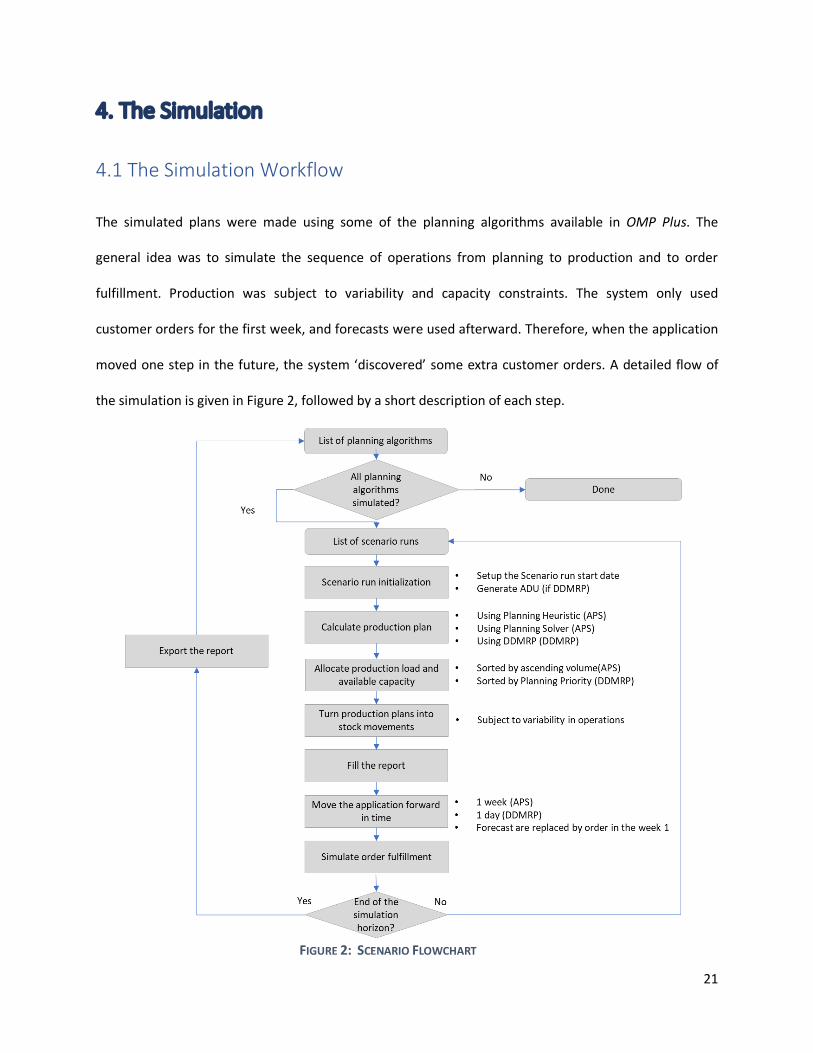
The simulated plans were made using some of the planning algorithms available in OMP Plus. The

general idea was to simulate the sequence of operations from planning to production and to order

fulfillment. Production was subject to variability and capacity constraints. The system only used

customer orders for the first week, and forecasts were used afterward. Therefore, when the application

moved one step in the future, the system ‘discovered’ some extra customer orders. A detailed flow of

the simulation is given in Figure 2, followed by a short description of each step.

FIGURE 2: SCENARIO FLOWCHART

22

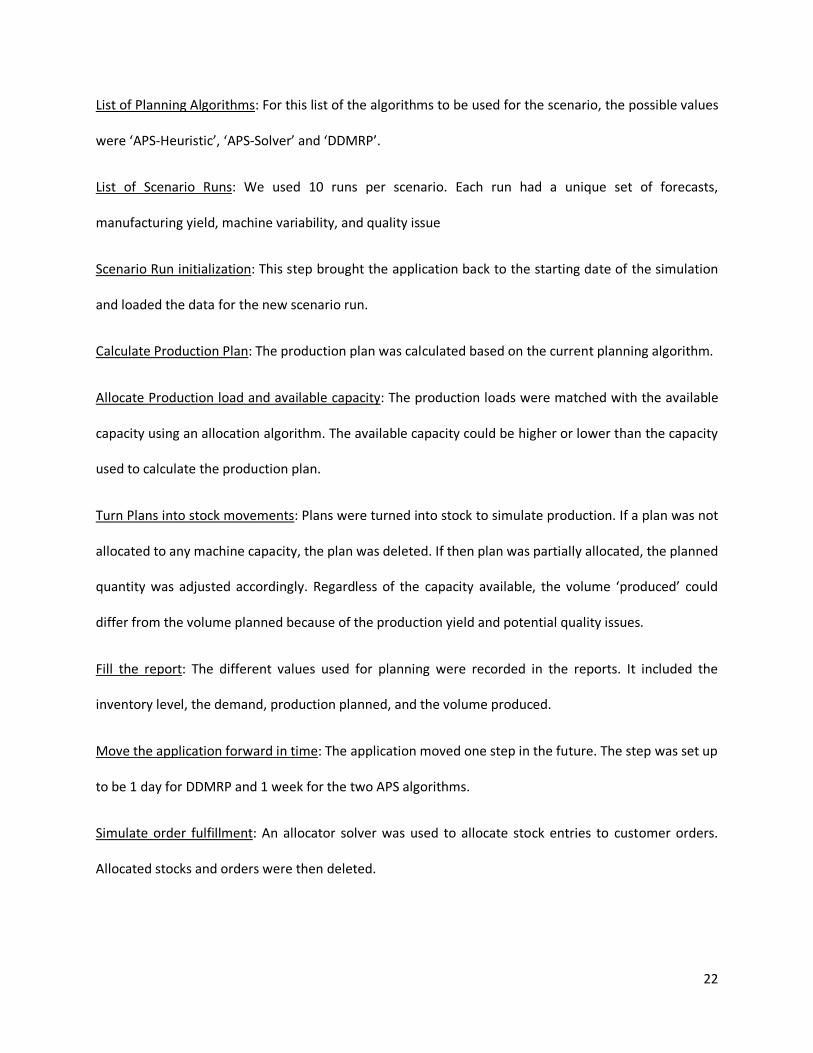
List of Planning Algorithms: For this list of the algorithms to be used for the scenario, the possible values

were ‘APS-Heuristic’, ‘APS-Solver’ and ‘DDMRP’.

List of Scenario Runs: We used 10 runs per scenario. Each run had a unique set of forecasts,

manufacturing yield, machine variability, and quality issue

Scenario Run initialization: This step brought the application back to the starting date of the simulation

and loaded the data for the new scenario run.

Calculate Production Plan: The production plan was calculated based on the current planning algorithm.

Allocate Production load and available capacity: The production loads were matched with the available

capacity using an allocation algorithm. The available capacity could be higher or lower than the capacity

used to calculate the production plan.

Turn Plans into stock movements: Plans were turned into stock to simulate production. If a plan was not

allocated to any machine capacity, the plan was deleted. If then plan was partially allocated, the planned

quantity was adjusted accordingly. Regardless of the capacity available, the volume ‘produced’ could

differ from the volume planned because of the production yield and potential quality issues.

Fill the report: The different values used for planning were recorded in the reports. It included the

inventory level, the demand, production planned, and the volume produced.

Move the application forward in time: The application moved one step in the future. The step was set up

to be 1 day for DDMRP and 1 week for the two APS algorithms.

Simulate order fulfillment: An allocator solver was used to allocate stock entries to customer orders.

Allocated stocks and orders were then deleted.

23

4.2 Description of the assumptions and the planning algorithms

This section describes the planning algorithms used and the different assumptions made to set up the

simulation model.

DDMRP inventory buffers are made of 3 zones. The green zone controls the order frequency and the

production batch size. The yellow zone provides the inventory required to cover the replenishment

time. The red zone protects the system against the variability. The values separating the different zones

of the buffers are called Top of Green, Top of Yellow and Top of Red.

The regular DDMRP calculation was used. If the Netflow Position in the first period was below the Top of

Yellow, a plan was created on the preferred machine at t = DLT (Decoupled Lead Time) in order to bring

the Netflow Position back to the Top of Green. A heuristic was run to spread the production volumes

across the available production lines.

In the case of an ‘APS-Heuristics’ a planning heuristic was used. Whenever the plan was falling below the

minimum inventory level, a plan was created to bring it back to the target level. Because the APS had a

one-week frozen horizon, the plan of the first week was never adjusted. The heuristic assigns the

preferred machine until it is overloaded, it then selects the next machine.

The assumptions for the simulation analysis were as follow:

- Assumptions 1: The priority rules for allocating the capacity

- Assumptions 2: No production splits

- Assumption 3: The order horizon

- Assumption 4: The frozen horizon of 1 week

- Assumption 5: No order lead time for raw material

24

Assumptions 1

Priorities on the production floors are usually complex. We simplified the current rules of the company.

In the case of APS algorithms, the priority was given to the smaller batches. Typically, the products of

larger batches are produced more frequently than the products of the smaller batches. Therefore, it is

better not to truncate the production of more frequently produced products.

In the case of a ‘DDMRP calculation’, the allocating algorithm gave priority to the production with the

highest buffer penetration. The buffer penetration is the ratio of the current Netflow Position divided by

the value of Top of Green.

Assumptions 2

The simulation also assumes that it is not possible to split production. For example, a planner could

decide to produce 85%, 85% and 75% of the requirements of 3 products instead of 100%, 100%, and

50%. The simulation did not include such logic.

Assumptions 3, 4 and 5

Assumption 3 and 4 will be discussed in Section 4.3.

4.3 Description of the company

The simulation analysis was applied for a food manufacturer operating in Europe. The company

produces perishable goods that can only be held for a couple of weeks in inventory. Due to the

perishability of the items, inventory turns are high, and the current inventory targets range from 1.6 to

2.5 weeks. The manufacturer typically receives orders from Monday to Thursday for the next week. We

simplified it by assuming that all the orders are received at once 1 week before (Assumption 3).

25

The company validates the production plan on Friday for the next week. Even though some minor

adjustments are possible on Monday, the first week of the production plan is frozen. The simulation did

not include any adjustment in the first week ( Assumption 4).

The company is part of a cooperative, which means that it has to inform the cooperative how much raw

material it will consume over the next 13 weeks. The sourcing plan is fixed for the next 4 weeks. Because

it is part of a cooperative, the company is frequently asked to take in more raw material than it needs.

These constraints were not included in the simulation because they are only relevant for tactical

planning and DDMRP focuses on operational planning. (Assumption 5)

26

5. Results

5.1 Qualitative and Quantitative Research Results

In this section, we will discuss the results of our survey responses and interviews to answer our research

question ‘What are the potential added values of DDMRP in planning under uncertainty at finite

capacity? ‘. Investigating the potential added value requires a clear view of the situation before the

implementation. Finally, we will explore the planning constraints faced by the respondents to better

understand what companies can benefit from a DDMRP implementation.

We received 109 responses out of which 27 responses have more than 65% of the questions answered.

The following analysis is based on these 27 responses and the 8 interviews that we conducted.

Overview of the Respondents

The respondents’ companies are diverse in term of annual revenues. About, 17% of the respondents

report an annual revenue lower than $100 million, while 46% report a revenue between $100 and $500

million. About 29% of the companies have a revenue exceeding $10 000 million.

From an industry point of view, companies coming from what we call ‘semi-process’ accounts for 56%.

Semi-Process industries are characterized by production of large batches of products packed in different

packaging. Table 3 gives the breakdown of the companies per industries.

TABLE 3: REPARTITION OF COMPANIES PER INDUSTRY

Industry Repartition FMCG/Life Sciences/Food & Dairy/Chemicals (Semi-Process) 56% Mechanical and Assembly 19% Mills and flow production 7% Other 19%

27

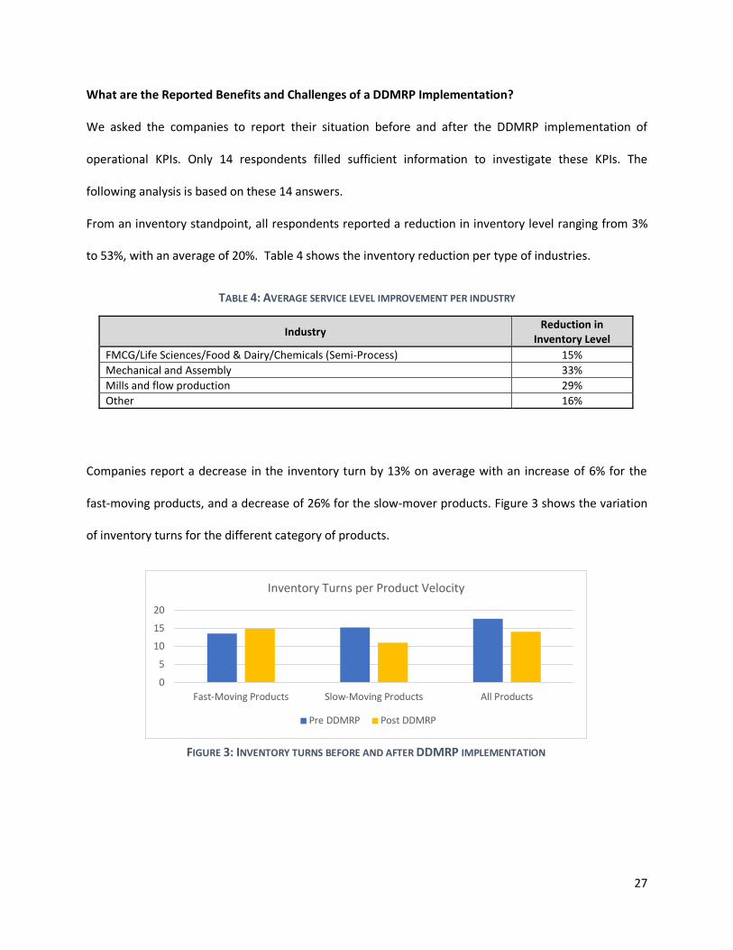
What are the Reported Benefits and Challenges of a DDMRP Implementation?

We asked the companies to report their situation before and after the DDMRP implementation of

operational KPIs. Only 14 respondents filled sufficient information to investigate these KPIs. The

following analysis is based on these 14 answers.

From an inventory standpoint, all respondents reported a reduction in inventory level ranging from 3%

to 53%, with an average of 20%. Table 4 shows the inventory reduction per type of industries.

TABLE 4: AVERAGE SERVICE LEVEL IMPROVEMENT PER INDUSTRY

Companies report a decrease in the inventory turn by 13% on average with an increase of 6% for the

fast-moving products, and a decrease of 26% for the slow-mover products. Figure 3 shows the variation

of inventory turns for the different category of products.

0

5

10

15

20

Fast-Moving Products Slow-Moving Products All Products

Inventory Turns per Product Velocity

Pre DDMRP Post DDMRP

FIGURE 3: INVENTORY TURNS BEFORE AND AFTER DDMRP IMPLEMENTATION

Industry Reduction in Inventory Level

FMCG/Life Sciences/Food & Dairy/Chemicals (Semi-Process) 15% Mechanical and Assembly 33% Mills and flow production 29% Other 16%

28

When respondents are asked about level of service achieved with their legacy system and DDMRP;

organizations report that they achieve better service levels after the implementation of DDMRP. The

average achieved service levels increased to 93% from 83%. The average improvement in service level,

calculated per company is 13%. It is higher than the overall improvement because companies with lower

initial service level report stronger improvements.

About 85% of the 26 respondents who answered the questions state that DDMRP improves planning

stability. About 92% of the companies report a better view of the priority and 69% states that DDMRP

enables them to have better control over the operations. Figure 4 shows the reported improvements in

the operations.

In order to achieve these improvements, 54% of the companies redesigned their supply chain by

changing what products should be held in stock at the different points of the supply chain. Among the

companies who changed their decoupling points, 93% had not investigated it before DDMRP, or they

had a long time ago. The concept of decoupling points is not new, but our data show that implementing

the demand driven approach leads to its usage in the companies. Table 5 summarizes the main benefits

of DDMRP on the operations.

FIGURE 4: IMPROVEMENTS IN THE OPERATIONS WITH DDMRP

29

TABLE 5: IMPACT OF DDMRP ON OPERATIONS FOR ALL COMPANIES

Operational Consideration Average change post DDMRP

Frequency of occurrence

Inventory level -20% - Inventory turns -13% - Service level 13% - Customer order lead time -48% - Repositioning of decoupling points in the supply chain - 54% More stable production schedule - 85% Better visibility in the priority 92%

Change management was mentioned in every interview as being the main challenge in implementing

DDMRP. All the interviewees claim that they had to train more people than they initially expected. They

trained people from different departments, from finance to manufacturing. Scaling-up DDMRP is

reported as difficult or moderately difficult by 85% of the surveyed companies.

What was the Situation Before DDMRP?

Of the survey respondents, 63% of the organizations implemented DDMRP directly from MRP while 37%

implemented DDMRP after implementing APS.

Table 6 gives an overview of the benefits of the DDMRP implementation broken down per legacy

systems. We can see that improvements are higher when companies come from MRP. DDMRP seems to

have a greater impact on planning stability and prioritization for the companies discontinuing an APS.

TABLE 6: IMPACT OF DDMRP ON OPERATIONS PER LEGACY SYSTEM

Operational Consideration Average change

coming from APS

Frequency of occurrence

coming from APS

Average change coming from

MRP

Frequency of occurrence coming

from MRP

Inventory level -13% - -23% - Inventory turns -23% - -7% - Service level 7% - 23% - Customer order lead time -26% - -55% - Repositioning of decoupling points in the supply chain - 10% - 76%

More stable production schedule - 90% - 81% Better visibility in the priority 90% 94%

30

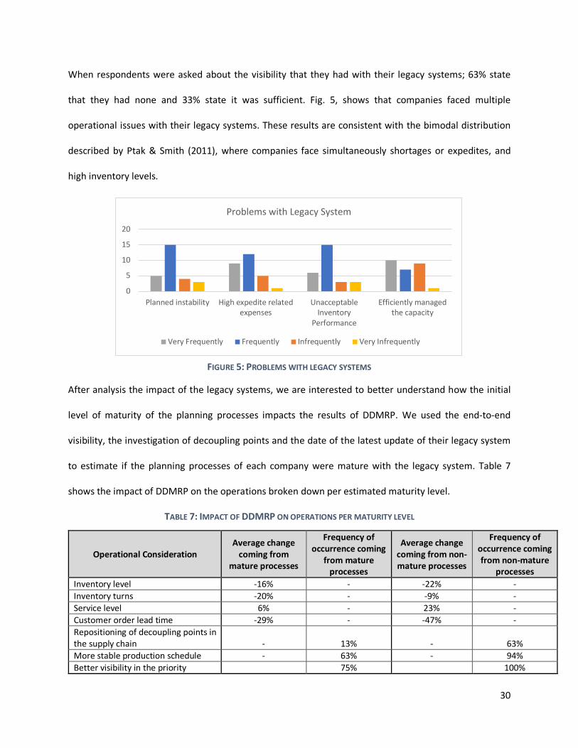
When respondents were asked about the visibility that they had with their legacy systems; 63% state

that they had none and 33% state it was sufficient. Fig. 5, shows that companies faced multiple

operational issues with their legacy systems. These results are consistent with the bimodal distribution

described by Ptak & Smith (2011), where companies face simultaneously shortages or expedites, and

high inventory levels.

After analysis the impact of the legacy systems, we are interested to better understand how the initial

level of maturity of the planning processes impacts the results of DDMRP. We used the end-to-end

visibility, the investigation of decoupling points and the date of the latest update of their legacy system

to estimate if the planning processes of each company were mature with the legacy system. Table 7

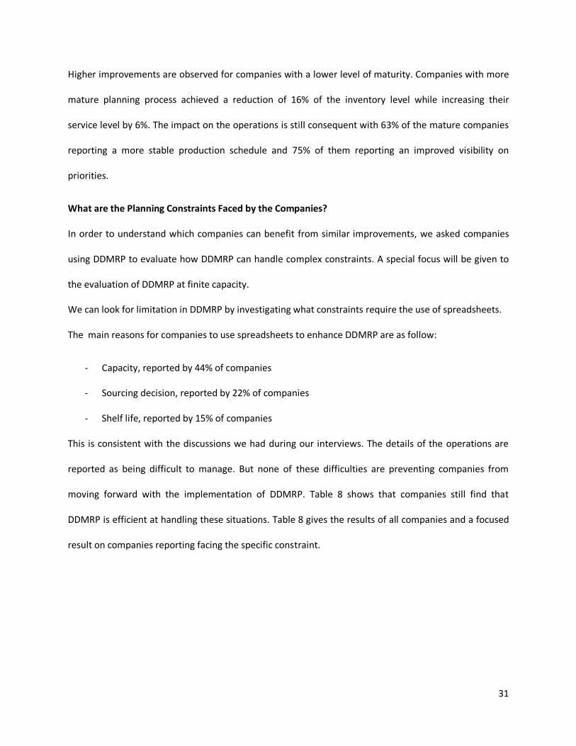
shows the impact of DDMRP on the operations broken down per estimated maturity level.

TABLE 7: IMPACT OF DDMRP ON OPERATIONS PER MATURITY LEVEL

Operational Consideration Average change

coming from mature processes

Frequency of occurrence coming

from mature processes

Average change coming from non-mature processes

Frequency of occurrence coming from non-mature

processes Inventory level -16% - -22% - Inventory turns -20% - -9% - Service level 6% - 23% - Customer order lead time -29% - -47% - Repositioning of decoupling points in the supply chain - 13% - 63% More stable production schedule - 63% - 94% Better visibility in the priority 75% 100%

FIGURE 5: PROBLEMS WITH LEGACY SYSTEMS

0

5

10

15

20

Planned instability High expedite relatedexpenses

UnacceptableInventory

Performance

Efficiently managedthe capacity

Problems with Legacy System

Very Frequently Frequently Infrequently Very Infrequently

31

Higher improvements are observed for companies with a lower level of maturity. Companies with more

mature planning process achieved a reduction of 16% of the inventory level while increasing their

service level by 6%. The impact on the operations is still consequent with 63% of the mature companies

reporting a more stable production schedule and 75% of them reporting an improved visibility on

priorities.

What are the Planning Constraints Faced by the Companies?

In order to understand which companies can benefit from similar improvements, we asked companies

using DDMRP to evaluate how DDMRP can handle complex constraints. A special focus will be given to

the evaluation of DDMRP at finite capacity.

We can look for limitation in DDMRP by investigating what constraints require the use of spreadsheets.

The main reasons for companies to use spreadsheets to enhance DDMRP are as follow:

- Capacity, reported by 44% of companies

- Sourcing decision, reported by 22% of companies

- Shelf life, reported by 15% of companies

This is consistent with the discussions we had during our interviews. The details of the operations are

reported as being difficult to manage. But none of these difficulties are preventing companies from

moving forward with the implementation of DDMRP. Table 8 shows that companies still find that

DDMRP is efficient at handling these situations. Table 8 gives the results of all companies and a focused

result on companies reporting facing the specific constraint.

32

TABLE 8: EFFECTIVENESS OF DDMRP

Effectiveness of DDMRP in planning at finite capacity Effectiveness of DDMRP in handling shelf-life limitation

All respondents Capacity constraints respondents All respondents Shelf-life constraints

respondents

Not effective 27% 9% Not effective 29% 10%

Moderately effective 15% 18% Moderately

effective 29% 20%

Effective 58% 73% Effective 42% 30% Effectiveness of DDMRP in handling sourcing decisions

All respondents Facing sourcing decisions respondents

Not effective 19% 15% Moderately effective 27% 38%

Effective 54% 46%

Our study shows that DDMRP is an effective planning approach at finite capacity. In our survey, 58% of

the respondents estimate DDMRP to be very effective or extremely effective at handling capacity

constraint, 15% of the respondents estimate it to be moderated effective, and 27% of them find it to be

slightly effective or not effective at all. It is noticeable that only 9% of the companies showing capacity

constraints report DDMRP has not effective at finite capacity, while 73% of them estimate it to be

effective.

All companies that we interviewed mentioned the difficulty to smooth out the capacity over the work

week. We experienced similar difficulties when we set up the simulation. Because DDMRP only

considers the situation of the current day, it can use only part of the available capacity on one day and

run out of capacity the next day. All the interviewed companies are experimenting with different options

to overcome this difficulty.

One of the interviewed companies mentioned that by reducing the inventory levels DDMRP frees up

capacity. This makes sense because inventory is capacity that is consumed in previous weeks. The

33

unexpected gain of capacity, according to this company, has a positive net impact on the available

capacity, despite the increases of time spent in setup.

5.2 Simulation Analysis Results

In this section, we discuss the results of our simulation. Each scenario was made of 10 runs. Each run is

evaluated in term of service level and inventory turns. The same customer orders were used for all

scenarios, which makes inventory turns comparable. Note that the planning parameters are not

changed between the different scenarios. This explains why the service levels drop as low as 80%. This

approach was selected to make it easy to understand the impact of the different situations on the

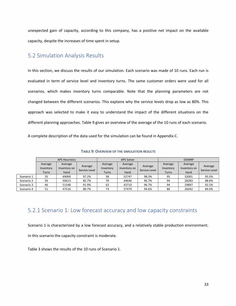
different planning approaches. Table 9 gives an overview of the average of the 10 runs of each scenario.

A complete description of the data used for the simulation can be found in Appendix C.

5.2.1 Scenario 1: Low forecast accuracy and low capacity constraints

Scenario 1 is characterized by a low forecast accuracy, and a relatively stable production environment.

In this scenario the capacity constraint is moderate.

Table 3 shows the results of the 10 runs of Scenario 1.

TABLE 9: OVERVIEW OF THE SIMULATION RESULTS

Average Inventory

Turns

Average Inventory on

hand

Average Service Level

Average Inventory

Turns


hand


Average Inventory

Turns


hand


Scenario 1 35 69000 97.2% 58 52747 98.3% 95 32001 95.5%Scenario 2 50 50613 85.7% 70 44646 96.7% 94 28283 88.6%Scenario 3 46 51548 91.9% 63 43710 96.7% 94 29897 92.5%Scenario 4 51 47516 80.7% 73 37470 94.6% 86 26042 84.0%

APS Heuristics DDMRPAPS Solver

34

In this simulation, we can see that with the used configuration of DDMRP, it gives a lower service level

than both algorithms of APS. In order to achieve this 1.7% service level improvement, the APS heuristic-

based planning requires 116% more inventory than DDMRP. The solver provides a service level

improved by 2.8% and requires 65% more inventory compared to DDMRP.

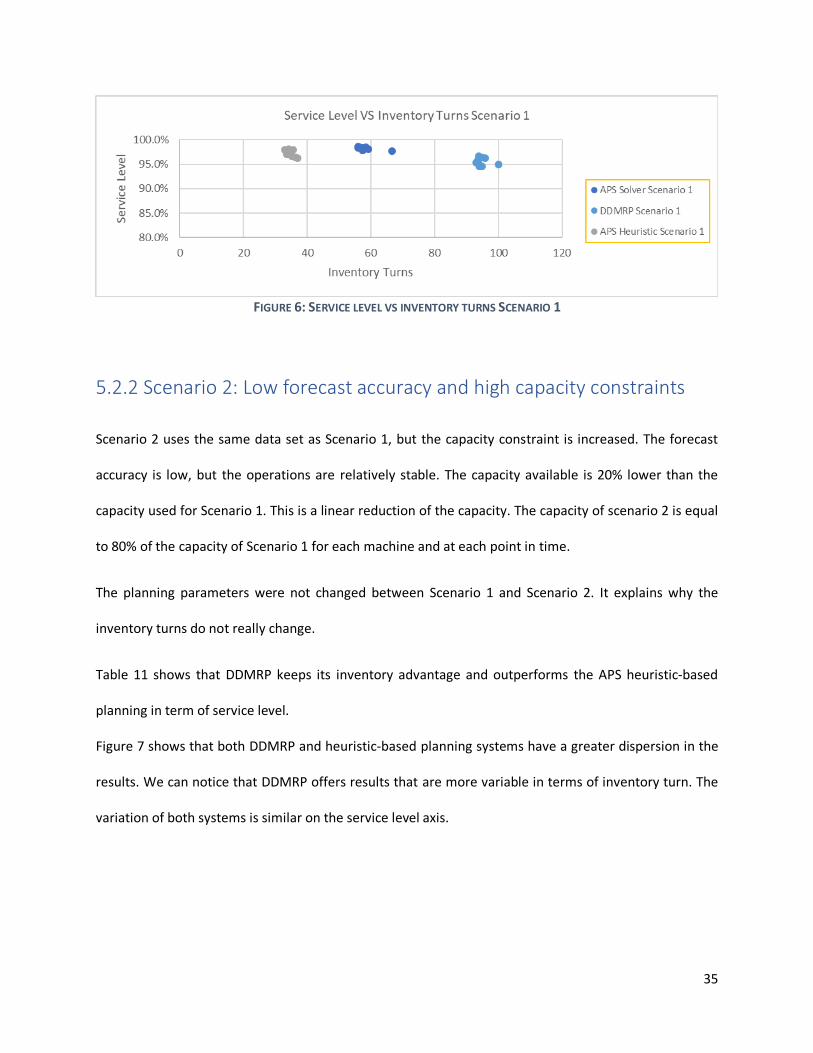
Figure 6 shows that all systems are stable at this level of variation. The solver-based planning delivers an

average inventory turn of 58 with a standard deviation of 3.11, and a service level of 98.3% with a

standard deviation of 0.29%. Figure 6 shows two very distinct clusters, which indicates that we can

expect different results from both systems.

Average Inventory Turnover

Average Inventory Level

Service LevelAverage

Inventory Turnover


Service LevelAverage

Inventory Turnover


Service Level

Run 1 34 70403 97.3% 58 55333 98.4% 93 33516 95.4%Run 2 34 68681 97.1% 58 51950 98.5% 95 31837 96.4%Run 3 35 65964 96.6% 67 58091 97.7% 93 31950 95.7%Run 4 34 70660 97.5% 57 51665 98.3% 95 31206 94.6%Run 5 33 71068 97.9% 56 53891 98.6% 94 32131 96.7%Run 6 37 65689 96.3% 59 50668 98.1% 100 31865 95.0%Run 7 34 71832 98.1% 56 52353 98.4% 94 33416 95.1%Run 8 34 68907 97.1% 57 51491 97.8% 96 31314 96.3%Run 9 35 71958 98.0% 56 52978 98.5% 94 31797 94.5%Run 10 36 64838 96.4% 57 49048 98.3% 94 30983 95.8%Average 35 69000 97.2% 58 52747 98.3% 95 32001 95.5%Standard Deviation

1.29 2654 0.66% 3.11 2542 0.29% 2.08 853 0.77%

Coefficient variation 0.037 0.038 0.007 0.054 0.048 0.003 0.022 0.027 0.008

APS Solver DDMRPAPS Heuristics

TABLE 10: SCENARIO 1 RESULTS

35

FIGURE 6: SERVICE LEVEL VS INVENTORY TURNS SCENARIO 1

5.2.2 Scenario 2: Low forecast accuracy and high capacity constraints

Scenario 2 uses the same data set as Scenario 1, but the capacity constraint is increased. The forecast

accuracy is low, but the operations are relatively stable. The capacity available is 20% lower than the

capacity used for Scenario 1. This is a linear reduction of the capacity. The capacity of scenario 2 is equal

to 80% of the capacity of Scenario 1 for each machine and at each point in time.

The planning parameters were not changed between Scenario 1 and Scenario 2. It explains why the

inventory turns do not really change.

Table 11 shows that DDMRP keeps its inventory advantage and outperforms the APS heuristic-based

planning in term of service level.

Figure 7 shows that both DDMRP and heuristic-based planning systems have a greater dispersion in the

results. We can notice that DDMRP offers results that are more variable in terms of inventory turn. The

variation of both systems is similar on the service level axis.

36

The solver-based planning offers the highest service level but requires 58% more inventory in

comparison with DDMRP. It presents a very low variance between the runs.

APS heuristic-based planning presents few results with similar service level, but a comparison run per

run shows that DDMRP is consistently achieving a higher service level.

FIGURE 7: SERVICE LEVELS VS INVENTORY TURNS SCENARIO 2


Average Inventory

LevelService Level


Average Inventory

LevelService Level


Average Inventory

LevelService Level

Run 1 51 49414 85.7% 72 43893 96.9% 86 28511 87.4%Run 2 52 51799 86.1% 69 42369 97.3% 97 26725 89.4%Run 3 52 48940 85.9% 67 42367 96.7% 98 29661 90.5%Run 4 50 49858 86.7% 70 43745 96.7% 88 27720 87.3%Run 5 50 48478 87.2% 71 43602 97.0% 100 26498 90.4%Run 6 48 51673 84.9% 72 45317 96.1% 94 28634 88.5%Run 7 50 52701 85.3% 66 45584 96.7% 98 27680 88.2%Run 8 46 51542 86.6% 70 47498 96.1% 95 29114 89.1%Run 9 51 50629 83.1% 68 48258 97.2% 91 30007 86.5%Run 10 50 51093 85.9% 69 43829 96.3%Average 50 50613 85.7% 70 44646 96.7% 94 28283 88.6%Standard Deviation

1.80 1388 1.13% 2.11 2001 0.43% 4.90 1227 1.39%

Coefficient variation

0.036 0.027 0.013 0.030 0.045 0.004 0.052 0.043 0.016

APS Heuristics APS Solver DDMRP


37

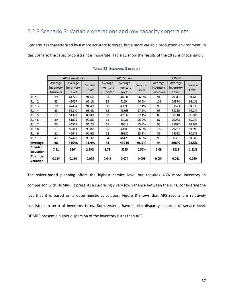
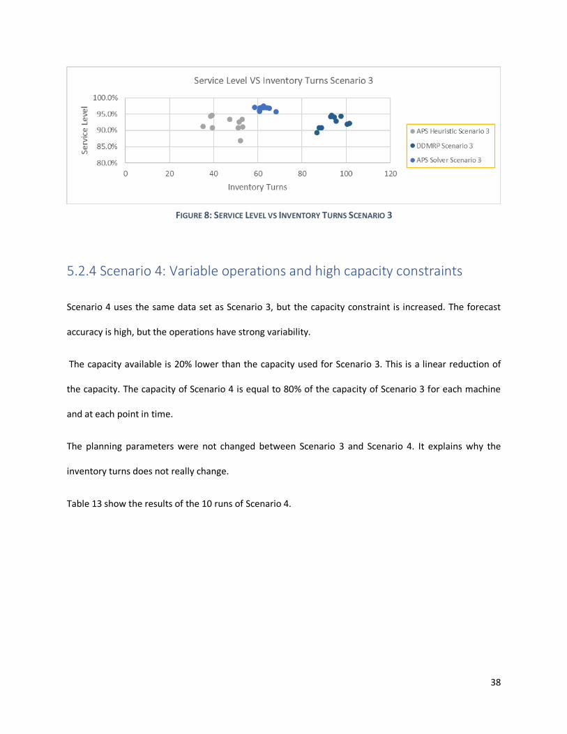
5.2.3 Scenario 3: Variable operations and low capacity constraints

Scenario 3 is characterized by a more accurate forecast, but a more variable production environment. In

this Scenario the capacity constraint is moderate. Table 12 show the results of the 10 runs of Scenario 3.


The solver-based planning offers the highest service level but requires 46% more inventory in

comparison with DDMRP. It presents a surprisingly very low variance between the runs, considering the

fact that it is based on a deterministic calculation. Figure 8 shows that APS results are relatively

consistent in term of inventory turns. Both systems have similar disparity in terms of service level.

DDMRP present a higher dispersion of the inventory turns than APS.


Average Inventory

Level

Service Level


Average Inventory

Level

Service Level


Average Inventory

Level

Service Level


7.11 5864 2.29% 2.72 3255 0.56% 5.09 1212 1.82%


0.154 0.114 0.025 0.043 0.074 0.006 0.054 0.041 0.020


38


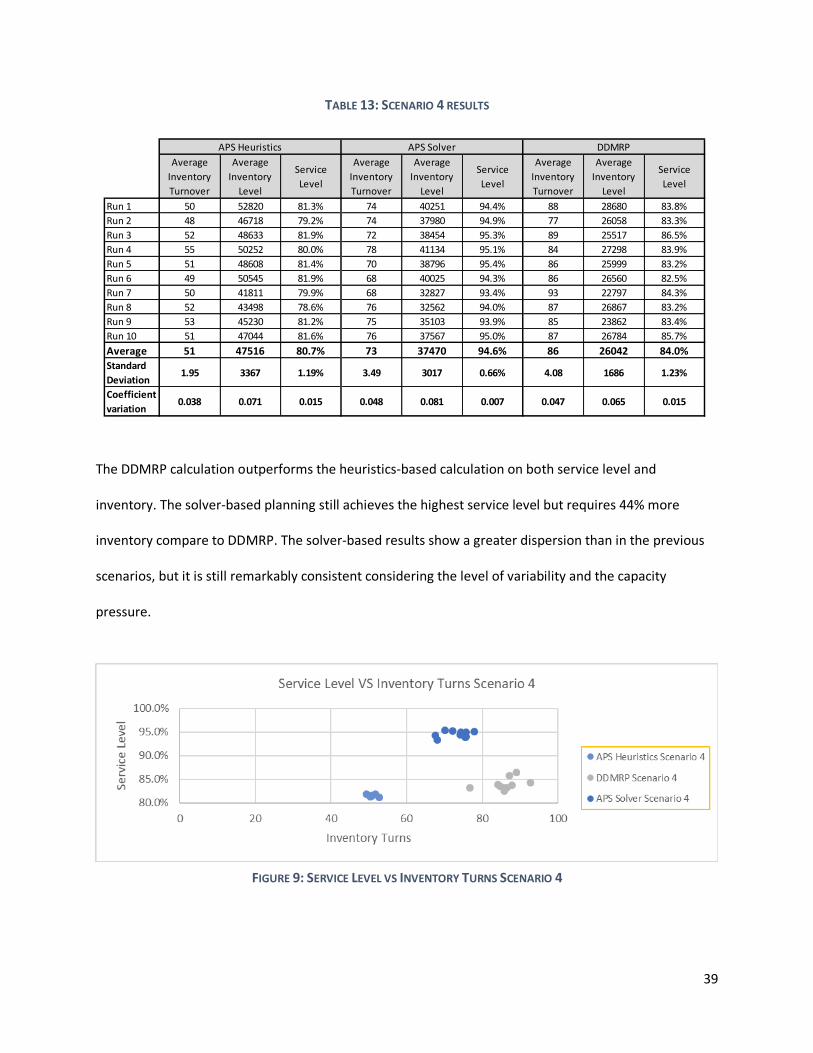
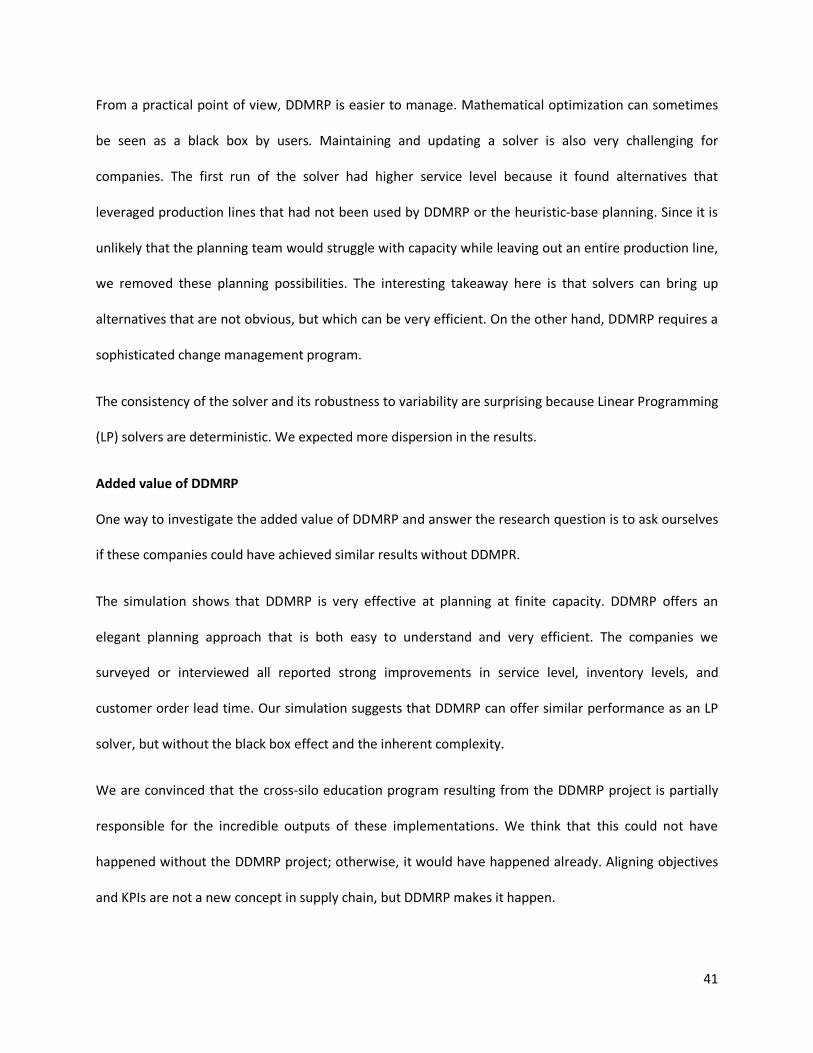
5.2.4 Scenario 4: Variable operations and high capacity constraints

Scenario 4 uses the same data set as Scenario 3, but the capacity constraint is increased. The forecast

accuracy is high, but the operations have strong variability.

The capacity available is 20% lower than the capacity used for Scenario 3. This is a linear reduction of

the capacity. The capacity of Scenario 4 is equal to 80% of the capacity of Scenario 3 for each machine

and at each point in time.

The planning parameters were not changed between Scenario 3 and Scenario 4. It explains why the

inventory turns does not really change.

Table 13 show the results of the 10 runs of Scenario 4.

39


The DDMRP calculation outperforms the heuristics-based calculation on both service level and

inventory. The solver-based planning still achieves the highest service level but requires 44% more

inventory compare to DDMRP. The solver-based results show a greater dispersion than in the previous

scenarios, but it is still remarkably consistent considering the level of variability and the capacity

pressure.



Average Inventory

Level

Service Level


Average Inventory

Level

Service Level


Average Inventory

Level

Service Level


1.95 3367 1.19% 3.49 3017 0.66% 4.08 1686 1.23%


0.038 0.071 0.015 0.048 0.081 0.007 0.047 0.065 0.015


40

6. Discussion

The qualitative and quantitative research clearly shows that companies implementing DDMRP have

observed improvements in their service level, inventory level, and customer lead time. These results are

consistent with the results of the simulation analysis.

DDMRP at finite capacity

The data collected through the survey and the interviews show that DDMRP has proven itself capable of

operating in capacity-constrained environments. However, smoothing out the capacity throughout the

week is more challenging than with other planning tools.

Our simulation also shows that DDMRP is robust and capable of handling variability. DDMRP’s

performance is less impacted by an increase in the variability or by capacity constraint than the

heuristic-based planning.

It is also important to point out that DDMRP is only one part of the Demand Driven Operating Model

(DDOM). The DDOM includes finite capacity control points to help balance machine loads.

Analyzing the difference between ‘conventional’ APS planning and DDMRP planning

DDMRP results show a strong resilience to the increase of variability or capacity constraint. DDMRP

performs better than the heuristics-based planning in all scenarios, except Scenario 1. In Scenario 1

DDMRP uses two times less inventory as the heuristic-based algorithms and is only lagging 1.7% behind

in terms of service level. The solver-based planning continually provides the highest service level, but it

requires higher inventory levels than DDMRP. Unfortunately, we did not have the opportunity to adjust

the DDMRP buffers to match up the service levels. This would have allowed us to compare the resulting

inventory levels. Based on the available results it is not possible to conclude whether the solver-based or

DDMRP performs better.

41

From a practical point of view, DDMRP is easier to manage. Mathematical optimization can sometimes

be seen as a black box by users. Maintaining and updating a solver is also very challenging for

companies. The first run of the solver had higher service level because it found alternatives that

leveraged production lines that had not been used by DDMRP or the heuristic-base planning. Since it is

unlikely that the planning team would struggle with capacity while leaving out an entire production line,

we removed these planning possibilities. The interesting takeaway here is that solvers can bring up

alternatives that are not obvious, but which can be very efficient. On the other hand, DDMRP requires a

sophisticated change management program.

The consistency of the solver and its robustness to variability are surprising because Linear Programming

(LP) solvers are deterministic. We expected more dispersion in the results.

Added value of DDMRP

One way to investigate the added value of DDMRP and answer the research question is to ask ourselves

if these companies could have achieved similar results without DDMPR.

The simulation shows that DDMRP is very effective at planning at finite capacity. DDMRP offers an

elegant planning approach that is both easy to understand and very efficient. The companies we

surveyed or interviewed all reported strong improvements in service level, inventory levels, and

customer order lead time. Our simulation suggests that DDMRP can offer similar performance as an LP

solver, but without the black box effect and the inherent complexity.

We are convinced that the cross-silo education program resulting from the DDMRP project is partially

responsible for the incredible outputs of these implementations. We think that this could not have

happened without the DDMRP project; otherwise, it would have happened already. Aligning objectives

and KPIs are not a new concept in supply chain, but DDMRP makes it happen.

42

Change management has been a central topic in our interviews and the surveyed companies frequently

mentioned it as one of the main challenges. We learned during the interviews and other conversations

outside the scope of this project that DDMRP calls for a comprehensive supply chain education program

within the companies. Every company had to train people from different functions, from finance to

manufacturing to procurement. We then realized that the DDMRP projects made these companies do

what all companies should do: align the different actors of the supply chain with the same objective.

Based on these interviews, and personal experience of the DDMRP training, we can say that these

companies trained the different actors of their internal supply chain to the basic concepts of flows, the

nature of the interactions between the different departments, and the importance of aligning the

decisions and the policies of the different functions. This is a real added value for the company, but it is

a challenging change management program, nevertheless. The panel of companies interviewed includes

several multi-billion-dollar companies. It is not the lack of internal knowledge or the costs of external

consultants that can explain why this focus on supply chain alignment has not happened previously.

We presume that the new set of proposed KPIs makes it harder to ignore the issues caused by a

misalignment in the operations. We also think that the way DDMRP is currently taught and implemented

strongly focuses on these questions. It is interesting to notice that MRP had similar effects at first. The

DDI and the different actors of the demand driven approaches will have to be very careful that this focus

does not erode over time.

In conclusion, even if the DDMRP results of our simulations are similar to the results of the solver-based

planning, we believe that the reported results could not be achieved without DDMRP. The alignment in

operations and the cross-silo collaboration resulting from the DDMRP implementation are key elements

for these success stories. Our qualitative and quantitative research analysis shows that DDMRP also

improves the operations in terms of planning stability and visibility. These are important features to

sustain high-level results from the operations.

43

Limitations of the study

In this project, we only interviewed and surveyed companies using DDMRP. Unfortunately, we could not

contact a company where DDMRP was explored but not pursued, or where the DDMRP implementation

failed. It would have been interesting to include the perspective of such companies.

We did not have the opportunity to optimize the buffer parameters in order to match up the service

level of DDMRP with the solver results. It would have been interesting to see if DDMRP could keep a

lower inventory, especially in the scenarios with high variability.

The simulation module does not include variance analysis to dynamically adjust the buffers when the

service level is too low. This is an important aspect of the system and our survey shows that 75% of the

companies use such feedback processes.

Our simulation does not fully cover a multi-tier supply chain. It is possible that DDMRP provides better

results since it will not use forecasts to replenish the different steps of the supply chain. We expect the

forecast errors to accumulate in the APS algorithms.

It would also be interesting to investigate the conversion of a company using a state-of-the-art APS to a

demand driven planning system. Some companies we interviewed had advanced planning processes and

systems before switching to DDMRP, but they were all MRP or basic APS. A real case study would be

very interesting because it is not possible to include all the operational constraints in the simulation. For

example, it is not possible to receive unexpected customer orders in the first week of our simulation.

This situation is possible and is known to cause operational issues.

44

7. Conclusion

In this project, we confirmed that companies using DDMRP achieve inventory reduction and increase

their service level simultaneously. These companies are also able to reduce their customer order lead

time by half. If payment terms are not changed, decreasing the inventory level reduces the working

capital and can increase the ROI of the company. The improved service level and the reduced customer

order lead time offer a competitive advantage. This competitive edge can result in higher revenue,

further improving the ROI.

According to our simulation analysis, DDMRP planning provides similar results as an advanced

mathematical solver and superior results compared to heuristic-based planning.

Moreover, our investigation also shows that implementing DDMRP forces the companies to develop an

extensive supply chain training program across the internal supply chain. All the interviewed companies

reported that DDMRP helps them to better streamline their operations.

Extending the simulation with a multi-echelon supply chain would be interesting. It would help to better

understand how forecast errors and production variability are transferred to the upper levels. Future

research could also create a case study of companies moving from a solver-based APS system to

DDMRP. Our simulation leaves out a number of operational constraints that only a real case study can

investigate.

This research proves that DDMRP can perform well in planning at finite capacity under uncertainty.

DDMRP can reduce the working capital and offer a competitive advantage, which gives DDMRP the

potential to be a game changer in supply chain planning.

45

References APICS, Blackston, J. (2015). APICS Dictionary, 15th Edition. Chicago: APICS, The Association for Operations Management. Blackburn, J. D., Kropp, D. H., & Millen, R. A. (1986). A comparison of strategies to dampen nervousness in MRP systems. Management Science, 53-60. Burbidge, J. (1980, October). What is wrong with materials requirement planning? Production Engineer, 59(10), pp. 57-59. Camelot (2019) Results of the Annual Demand-Driven SCM Survey. Retrieved from https://www.camelot-mc.com/wp-content/uploads/2019/03/Results-of-the-Annual-Demand-Driven-SCM-Survey_Christophe-Hudelmaier_CAMELOT-1.pdf Carlson, R. C., Jucker, J. V., & Kropp, D. (1979). Less nervous MRP systems: a dynamic economic lot sizing approach. Management Science, 745 - 761. Ptak, C. and Smith, S. (2011). DDMRP: Demand Driven Material Requirement Planning. Industrial Press, c2011 Ptak, C. and Smith, C. (2017). Precisely Wrong: Why Conventional Planning Systems Fail. Industrial Press, c2017 Smith, D. and Smith, C. (2013). Demand Driven Performance using Smart metrics. Mc Graw Hill, c2013 Eroglu, Cuneyt, and Hofer, C. (2011). “Lean, Leaner, Too Lean? The Inventory-Performance Link Revisited.” Journal of Operations Management 29, no. 4. 356–69. https://doi.org/10.1016/j.jom.2010.05.002. Funk, G. L. (2001). Enterprise integration: join the successful 20%. Hydrocarbon Processing, 43-46. Genin, P., Thomas, A., & Lamouri, S. (2007). How to manage robust planning with an APS. Springer Science + Business Media, 209-221.

46

Gruat-La-Forme, F. A., Botta-Genoulaz, V., Campagne, J.-P., & Millet, P.-A. (2005). Advance Planning and Scheduling system: An overview of gaps and potential sample solutions. International Conference on Industrial Engineering and Systems Management, 683-695. Heisig, D. G. (2002). Planning Stability in Material Requirements Planning Systems. Berlin: Springer, Berlin, Heidelberg. Ho, C.-J., Law, W.-K., & Rampal, R. (1995). Uncertainty-Dampening Methods for Reducing MRP System Nervousness. The International Journal of Production Research, 483-496. Hvolby, H.-H., & Steger-Jensen, K. (2010). Technical and Industrial Issues of Advance Planning and Scheduling (APS) Systems. Computers in Industry, 845-851. Kortabarria, Alaitz, Apaolaza, U., Lizarralde,A. , and Amorrortu, I. , (2018). Material Management without Forecasting: From MRP to Demand Driven MRP. Journal of Industrial Engineering and Management 11, no. 4. 632–50. https://doi.org/10.3926/jiem.2654. McCullen, P., and Eagle, S. (2015). Demand-Driven Innovation in Material Planning and Control: A review of early implementations. McNair, Carol J., Richard L. Lynch, and Kelvin F. Cross (1990). Do Financial and Nonfinancial Performance Measures Have to Agree? Management Accounting 72, no. 5, 28. Miclo, R., Fontanili, F., Lauras, M., Lamothe, J., & Milian, B. (2016). An empirical comparison of MRPII and Demand Driven MRP. International Federation of Automatic Control (pp. 1725-1730). IFAC-PapersOnline. Minifie, J. R., & Davis, R. A. (1990). Interaction effects on MRP nervousness. International Journal of Production Research, 173-183. Moscoso, P. G., Fransoo, J. C., & Fischer, D. (2010). An empirical study on reducing planning instability in hierarchical planning systems. Production Planning and Control, 413-426. New, C. (1975). Safety stocks for requirement planning. Production and Inventory Management, 1-18.

47

Obermaier, R., and Andreas Donhauser, A. (2012). Zero Inventory and Firm Performance: A Management Paradigm Revisited. International Journal of Production Research 50, no. 16. 4543–55. https://doi.org/10.1080/00207543.2011.613869. Orlicky, J. A. (1975). Materials Requirement Planning. New York: McGraw-Hill. Plossl, George W., (1918). Managing in the new world of manufacturing: How companies can improve operations to compete globally. Englewood Cliffs, NJ. Prentice Hall, c1991. Ptak, & Smith. (2011). Orlicky's Materials Requirement Planning (Vol. Third Edition). United States of America: Mc-Graw Hill. Shofa, M. J., & Widyarto, W. O. (2017). Effective production control in an automative industry: MRP vs DDMRP. AIP Conference Proceedings. American Institute of Physics. Shofa, M., Moeis, A., & Restiana, N. (2018). Effective production planning for purchased part under long lead time and uncertain demand: MRP vs demand-driven MRP. International Conference on Industrial and Systems Engineering. IOP Conf. Series: Materials Science and Engineering. Sridharan, V., and LaForge, R. L. (1990). “On Using Buffer Stock to Combat Schedule Instability.” International Journal of Operations & Production Management 10, no. 7. 37–46. Tempelmier, H. (2001). Supply Chain Planning with Advanced Planning Systems. Proceedings of the 3rd Aegean International Conference on Design and Analysis of Manufacturing Systems. Whybark, D. C., & Williams, J. G. (1976). Materials requirement planning under uncertainity. Decision Sciences, 595-606.

48

Appendix A – Interview Questions

Question # Topic Detailed points to investigate Priority

Full scope? Limited Product Families? All BU?How many products and locations?How long is it running?Motivation OptionalWhat were the expectations go fastKPIs to improve to be detailedDid you have a precise business case? To go in depth

Was it structured around an IT System?Was it mere MRP or APS?Did it offred sufficient SC visibility

What was your bigest operartion struggle? Costs, reliability, Service Level, instability?

4Did you carefully investigate where to hold inventory in your supply chain?

Work structure and methodsLevel of ServiceInventory level and runsROIs

6 Was there expectation not met with DDMRP?7 DDMRP offer a good end-to-end SC visibility?

MOQ or aggregated MOQCapacity constraintsSourcing decisionAlternative for productionShelflife Reduced variability in the upper levels?More stable planning and operationsin procurement

10 Do you use Excel Spreadsheet to include left-out constraints?11 Does DDMRP offers sufficient End-To-End visibility?

So you have examples?Do you feel you have more control over the operation?

Is it full DDS&OP?

Is it easy to work with? Easy to find the right new value? Not too time intensive?

What is the horizon?

What is the bucket of time used?Do you have issues within these buckets of time?For DDMRP?For capacity and demand balancingFor (DD)S&OPIs it efficient?Is it easy to scale up?Is there blind splot or missing warning?

You personallyMembers of the project Team?Planners?

18 What was the hardest thing to get over while deciding to go for DDMRP

19What was the hardest thing to get over while implementing to go for DDMRP

20 Did you use simulation to prepare the DDMRP module?Did you find similare results after the implementation for the scope of the simulation?

21 For you, what is the main added value of DDMRP?

22For you, what was the main surprise in the results of DDMRP POC or implementation?

23 For you what is the main drawback or limitation of DDMRP?

Did you learn a lot about Supply chain during DDMRP trainings?

Can DDMRP handle all of operational constraints?

Do you use the priority framework proposed by the DDI?

Prior DDMRP

Scope of DDMRP - for how long have they been running DDMRP.

Why did you decide to implement DDMRP?

What benefit/difference did they note with DDMRP

14

13

8

5

Do you feel DDMRP stabilized the supply chain?

Do you think DDMRP deliver more relevant informations

9

Set the stage. Understand the company

Implementing DDMRP

Conclusion

16

17

12

Working with DDMRP

Post DDMRP

What was your legacy system

Do you have a clear and structured way of adjusting buffers to anticipated events?

Do you have an active process to ensure that Supply and demand are in balance?

Did you implementated any systemic feedback loops?

1

2

3

15

49

Appendix B: Survey Questions

Section 1 Pre-DDMRP Implementation

1 What was your company's legacy Planning and Scheduling System? (Legacy system is the system you used to plan your supply chain before implementing DDMRP)

2

Did your Legacy system give you clear view of the state of inventory levels, expected demand, and capacity utilization throughout your supply chain and the impact of planning decisions made in the system? (Legacy system is the system you used to plan your supply chain before implementing DDMRP)

3.1

With your legacy system, did your company ever face the following scenarios? (Legacy system is the system you used to plan your supply chain before implementing DDMRP) - Planned instability i.e. changing priorities, raw material requirements and worker loads

3.2

With your legacy system, did your company ever face the following scenarios? (Legacy system is the system you used to plan your supply chain before implementing DDMRP) - High expedite related expenses i.e. freight, overtime, penalties

3.3

With your legacy system, did your company ever face the following scenarios? (Legacy system is the system you used to plan your supply chain before implementing DDMRP) - Unacceptable Inventory Performance

3.4

With your legacy system, did your company ever face the following scenarios? (Legacy system is the system you used to plan your supply chain before implementing DDMRP) - Efficiently managed the capacity

4.1 What was your annual average inventory turns? (If you don't have the answer please leave the slider at zero) - Fast Moving Products

4.2 What was your annual average inventory turns? (If you don't have the answer please leave the slider at zero) - Slow Moving Products

4.3 What was your annual average inventory turns? (If you don't have the answer please leave the slider at zero) - Average Inventory Turns for all of the products

5 Before learning about DDMRP, did your company carefully investigate where to place inventory and decoupling points?

6

When was the last time you upgraded or re-designed your legacy system ? (If you don't have the answer please leave the slider at zero) - No of Years

Section 2 Post DDMRP Implementation

1

Can you estimate the level of service, expressed as percentage, observed before and after the implementation of DDMRP? (If you don't have the answer, please leave the slider at zero) - Service Level before DDMRP Implementation

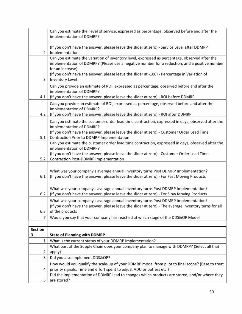
50

2

Can you estimate the level of service, expressed as percentage, observed before and after the implementation of DDMRP? (If you don't have the answer, please leave the slider at zero) - Service Level after DDMRP Implementation

3

Can you estimate the variation of inventory level, expressed as percentage, observed after the implementation of DDMRP? (Please use a negative number for a reduction, and a positive number for an increase) (If you don't have the answer, please leave the slider at -100) - Percentage in Variation of Inventory Level

4.1

Can you provide an estimate of ROI, expressed as percentage, observed before and after the implementation of DDMRP? (If you don't have the answer, please leave the slider at zero) - ROI before DDMRP

4.2

Can you provide an estimate of ROI, expressed as percentage, observed before and after the implementation of DDMRP? (If you don't have the answer, please leave the slider at zero) - ROI after DDMRP

5.1

Can you estimate the customer order lead time contraction, expressed in days, observed after the implementation of DDMRP? (If you don't have the answer, please leave the slider at zero) - Customer Order Lead Time Contraction Prior to DDMRP Implementation

5.2

Can you estimate the customer order lead time contraction, expressed in days, observed after the implementation of DDMRP? (If you don't have the answer, please leave the slider at zero) - Customer Order Lead Time Contraction Post-DDMRP Implementation

6.1 What was your company's average annual inventory turns Post DDMRP Implementation? (If you don't have the answer, please leave the slider at zero) - For Fast Moving Products

6.2 What was your company's average annual inventory turns Post DDMRP Implementation? (If you don't have the answer, please leave the slider at zero) - For Slow Moving Products

6.3

What was your company's average annual inventory turns Post DDMRP Implementation? (If you don't have the answer, please leave the slider at zero) - The average inventory turns for all of the products

7 Would you say that your company has reached at which stage of the DDS&OP Model Section 3 State of Planning with DDMRP

1 What is the current status of your DDMRP Implementation?

2 What part of the Supply Chain does your company plan to manage with DDMRP? (Select all that apply)

3 Did you also implement DDS&OP?

4 How would you qualify the scale-up of your DDMRP model from pilot to final scope? (Ease to treat priority signals, Time and effort spent to adjust ADU or buffers etc.)

5 Did the implementation of DDMRP lead to changes which products are stored, and/or where they are stored?

51

6.1 After implementing DDMRP, how would you rate the affirmation that your company has a systematic process to - Adjust the buffers according to past events (Feedback Loop)

6.2 After implementing DDMRP, how would you rate the affirmation that your company has a systematic process to - Adjust the buffers according to known, or anticipated future events

7 Does your company use spreadsheets to enhance DDMRP (handling extra planning constraints)? 8 Can you select constraints which are managed with spreadsheets? - Selected Choice

9.1 Please rate the effectiveness of DDMRP (that has been observed in your company) for the following - Planning at Finite Capacity

9.2 Please rate the effectiveness of DDMRP (that has been observed in your company) for the following - Handling sourcing decisions

9.3 Please rate the effectiveness of DDMRP (that has been observed in your company) for the following - Handling shelf-life constraints

10.1 Please rate to which degree you agree or disagree with the following statements? - Planning and scheduling are more stable with DDMRP

10.2 Please rate to which degree you agree or disagree with the following statements? - DDMRP gives your company a clearer view on priorities

10.3 Please rate to which degree you agree or disagree with the following statements? - DDMRP has offered more control over operations

10.4 Please rate to which degree you agree or disagree with the following statements? - DDMRP has made dependent requirements smoother

10.5 Please rate to which degree you agree or disagree with the following statements? - DDMRP provides your company with more relevant information

Section 4 About the company

1 What is your Company's core business? - Selected Choice 2 How many employees are there in your Company? 3 What is your Company's Annual Revenue (In Million Dollars)? 4 What primary type of production and stock management do you use? (Select all that apply)

5 Select the most relevant constraints you feel are the most important in your Supply Chain? Please do not select more than five constraints - Selected Choice

6 Do you have shelf-life constraints? 7 Can some of your products be produced in multiple factories or in multiple production lines? 8 Can your supply planner make a sourcing decision or is it an S&OP decision? 9 Can you provide an estimation of the number of SKUs that you are actively planning?

10.1 How would you qualify the demand variability of: - Most of your products

10.2 How would you qualify the demand variability of: - Poor performing products (level of service, stock level)

11 How would you qualify the supply variability of most of your components (lead time variability, quantity reliability)

12 Briefly explain what you think is the main added value of DDMRP? 13 Briefly explain what you think is the main limitation or drawback of DDMRP? 14 Please indicate if you would like to participate in a follow-up interview?

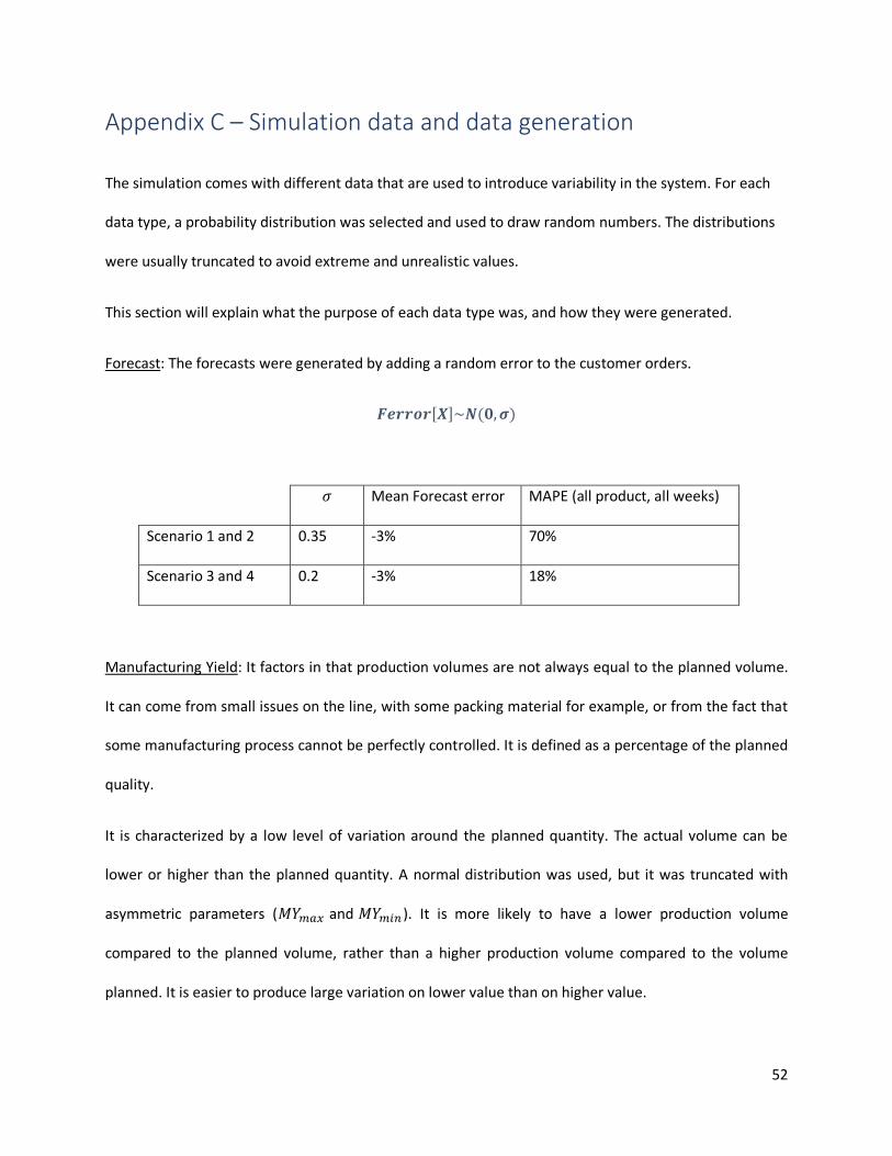
52

Appendix C – Simulation data and data generation

The simulation comes with different data that are used to introduce variability in the system. For each

data type, a probability distribution was selected and used to draw random numbers. The distributions

were usually truncated to avoid extreme and unrealistic values.

This section will explain what the purpose of each data type was, and how they were generated.

Forecast: The forecasts were generated by adding a random error to the customer orders.

𝑭𝒆𝒓𝒓𝒐𝒓[𝑿]~𝑵(𝟎,𝝈)

𝜎 Mean Forecast error MAPE (all product, all weeks)

Scenario 1 and 2 0.35 -3% 70%

Scenario 3 and 4 0.2 -3% 18%

Manufacturing Yield: It factors in that production volumes are not always equal to the planned volume.

It can come from small issues on the line, with some packing material for example, or from the fact that

some manufacturing process cannot be perfectly controlled. It is defined as a percentage of the planned

quality.

It is characterized by a low level of variation around the planned quantity. The actual volume can be

lower or higher than the planned quantity. A normal distribution was used, but it was truncated with

asymmetric parameters (𝑀𝑌234 and 𝑀𝑌256 ). It is more likely to have a lower production volume

compared to the planned volume, rather than a higher production volume compared to the volume

planned. It is easier to produce large variation on lower value than on higher value.

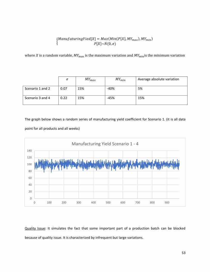
53

7𝑀𝑎𝑛𝑢𝑓𝑎𝑡𝑢𝑟𝑖𝑛𝑔𝑌𝑖𝑒𝑑[𝑋] = 𝑀𝑎𝑥(𝑀𝑖𝑛(𝑃[𝑋],𝑀𝑌234),𝑀𝑌256)𝑃[𝑋]~𝑁(0, 𝜎)

where𝑋isarandomvariable,𝑀𝑌WXYisthemaximumvariationand𝑀𝑌W]^istheminimumvariation

𝜎 𝑀𝑌234 𝑀𝑌256 Average absolute variation

Scenario 1 and 2 0.07 15% -40% 5%

Scenario 3 and 4 0.22 15% -45% 15%

The graph below shows a random series of manufacturing yield coefficient for Scenario 1. (it is all data

point for all products and all weeks)

Quality Issue: It simulates the fact that some important part of a production batch can be blocked

because of quality issue. It is characterized by infrequent but large variations.

0

20

40

60

80

100

120

140

0 100 200 300 400 500 600 700 800 900

Manufacturing Yield Scenario 1 - 4

54

A beta function was used. It was truncated to keep the coefficient between 0% and 100%

7𝑄𝑢𝑎𝑙𝑖𝑡𝑦𝐼𝑠𝑠𝑢𝑒[𝑋] = 𝑀𝑎𝑥(𝑀𝑖𝑛(𝑃[𝑋], 1,0) ∗ 100𝑃[𝑋]~𝛽(𝛼, 𝛽)

𝛼 𝛽 Mean Loss Mean loss per event

Scenario 1 and 2 0.012 0.45 -3% -20%

Scenario 3 and 4 0.012 0.45 -3% -20%

Machine Variability: This factor combines two concepts. The fact that the rates and available capacity

will fluctuate around the average, and more serious breakdowns. The first is characterized by small

autocorrelated variations around the mean. We modeled it as a pink noise. It is calculated by taking the

average over 7 random values (𝑃𝑅𝑉5) of a truncated normal distribution (𝑃𝑅𝑉𝑚𝑖𝑛 and 𝑃𝑅𝑉𝑚𝑎𝑥).

The average creates a smoothing effect to avoid that the capacity jump from low to very high. Rapid

changes are possible, but usually over a certain number of periods

0

20

40

60

80

100

120

0 200 400 600 800 1000 1200

Quality Issue factors

55

The second is characterized by infrequent but large variations. A beta contracted (𝑀𝐵𝑚𝑎𝑥) distribution

was used for this factor.

⎩⎪⎨

⎪⎧𝑀𝑎𝑐ℎ𝑖𝑛𝑒𝐴𝑣𝑎𝑖𝑙𝑎𝑏𝑖𝑙𝑖𝑡𝑦[𝑋] = (1 −𝑀𝑎𝑐ℎ𝑖𝑛𝑒𝐵𝑟𝑒𝑎𝑘𝐷𝑜𝑤𝑛[𝑋]) ∗ (1 + 𝑃𝑟𝑜𝑑𝑢𝑐𝑡𝑖𝑜𝑛𝑅𝑎𝑡𝑒𝑉𝑎𝑟𝑖𝑎𝑏𝑖𝑙𝑖𝑡𝑦[𝑋])𝑀𝑎𝑐ℎ𝑖𝑛𝑒𝐵𝑟𝑒𝑎𝑘𝐷𝑜𝑤𝑛[𝑋] = 𝑀𝑖𝑛(𝑀𝑎𝑥(𝑀𝐵[𝑋], 0), 𝐵𝑀234)|𝑀𝐵[𝑋]~𝛽(𝛼, 𝛽)

𝑃𝑟𝑜𝑑𝑢𝑐𝑡𝑖𝑜𝑛𝑅𝑎𝑡𝑒𝑉𝑎𝑟𝑖𝑎𝑏𝑖𝑙𝑖𝑡𝑦 = 18∗}𝑀𝑖𝑛(𝑀𝑎𝑥(𝑃𝑅𝑉5[𝑋], 𝑃𝑅𝑉256), 𝑃𝑅𝑉234)|𝑃𝑅𝑉[𝑋]~𝑁(0, 𝜎)

~

5��

𝑤ℎ𝑒𝑟𝑒𝑋𝑖𝑠𝑎𝑟𝑎𝑛𝑑𝑜𝑚𝑣𝑎𝑟𝑖𝑎𝑏𝑙𝑒, 𝐵𝑀234𝑖𝑠𝑡ℎ𝑒𝑚𝑎𝑥𝑖𝑚𝑢𝑚𝑙𝑜𝑠𝑠𝑑𝑢𝑒𝑡𝑜𝑚𝑎𝑐ℎ𝑖𝑛𝑒𝑏𝑟𝑒𝑎𝑘𝑑𝑜𝑤𝑛,

𝑃𝑅𝑉256𝑎𝑛𝑑𝑃𝑅𝑉𝑚𝑖𝑛𝑃𝑅𝑉234𝑎𝑟𝑒𝑡ℎ𝑒𝑚𝑖𝑛𝑖𝑚𝑢𝑚𝑎𝑛𝑑𝑚𝑎𝑥𝑖𝑚𝑢𝑚𝑣𝑎𝑟𝑖𝑎𝑡𝑖𝑜𝑛𝑓𝑟𝑜𝑚𝑝𝑟𝑜𝑑𝑢𝑐𝑡𝑖𝑜𝑛𝑟𝑎𝑡𝑒𝑣𝑎𝑟𝑖𝑎𝑡𝑖𝑜𝑛.

𝛼 𝛽 𝜎 𝑀𝐵𝑚𝑎𝑥 𝑃𝑅𝑉𝑚𝑎𝑥 𝑃𝑅𝑉𝑚𝑖𝑛 Mean Mach. Avail

Scenario 1 and 2 0.05 2 0.1 35% 15% -25% 96%

Scenario 3 and 4 0.09 3 0.65 50% 15% -40% 88.4%

0

20

40

60

80

100

120

140

0 50 100 150 200 250 300 350

Machine availability

Leo Ducrot Master of engineering, Institut Catholique d ...

Documents

Transcript of Leo Ducrot Master of engineering, Institut Catholique d ...