Lending Relationships and Optimal Monetary Policy

WP 20-13 Zachary BethuneUniversity of Virginia

Guillaume RocheteauUniversity of California, Irvine

Tsz-Nga WongFederal Reserve Bank of Richmond

Cathy ZhangPurdue University

Lending Relationships and Optimal Monetary Policy∗

Zachary BethuneUniversity of Virginia

Guillaume RocheteauUniversity of California, IrvineLEMMA, University of Paris II

Tsz-Nga WongFederal Reserve Bank of Richmond

Cathy ZhangPurdue University

This revised version: May 2020

Abstract

We construct and calibrate a monetary model of corporate finance with endogenous formationof lending relationships. The equilibrium features money demands by firms that depend on theiraccess to credit and a pecking order of financing means. We describe the mechanism throughwhich monetary policy affects the creation of relationships and firms’incentives to use internalor external finance. We study optimal monetary policy following an unanticipated destructionof relationships under different commitment assumptions. The Ramsey solution uses forwardguidance to expedite creation of new relationships by committing to raise the user cost of cashgradually above its long-run value. Absent commitment, the user cost is kept low, delayingrecovery.

JEL Classification: D83, E32, E51Keywords: Credit relationships, banks, corporate finance, optimal monetary policy.

∗We are grateful to Pietro Grandi for assistance and discussions on the data and empirical analysis. We alsothank Timothy Bond, Edouard Challe, Joshua Chan, Doug Diamond, Lucas Herrenbrueck, Mohitosh Kejriwal, Se-bastien Lotz, Fernando Martin, Katheryn Russ, Neil Wallace, Randy Wright, and Yu Zhu for comments, as wellas conference and seminar participants at the 2017 Money, Banking, and Asset Markets Workshop at University ofWisconsin in Madison, 2017 Summer Workshop on Money and Banking, 2017 Society of Economic Dynamics Meet-ings, 2017 Shanghai Workshop on Money and Finance, Indiana University, London School of Economics, U.C. Irvine,Peking University, Purdue University, Queens University, Virginia Tech, University of British Columbia, Universityof Western Ontario, University of Saskatchewan, Bank of Canada, and the Federal Reserve Banks of Kansas City andRichmond. Emails: zab2t@virginia.edu; grochete@uci.edu; russell.wong@rich.frb.org; cmzhang@purdue.edu. Theviews expressed in this paper are those of the authors and not necessarily those of the Federal Reserve Bank ofRichmond, or the Federal Reserve System.

1 Introduction

Most businesses, especially small ones, rely on secure access to credit through stable relationships

with banks. According to the 2003 Survey of Small Business Finances, 68% had access to a credit

line or revolving credit arrangement —a proxy for lending relationships. As documented in Section

2, these firms hold 20% less cash relative to firms that are not in a lending relationship, thereby

suggesting some degree of substituability between internal finance with cash and external finance

through banking relationships. Similarly, Compustat firms with access to a credit line hold 58%

less cash relative to firms without access. Insofar as monetary policy affects the user cost of cash,

these observations suggest an asymmetric transmission of monetary policy to firms depending on

their access to lending relationships.

Monetary policy transmission to relationship lending is especially critical in times of financial

crisis as a fraction of these relationships gets destroyed due to bank failures, stricter application

of loan covenants, or tighter lending standards.1 During the Great Depression, the destruction

of lending relationships explained one-eighth of the economic contraction (Cohen, Hachem, and

Richardson 2016). The goal of this paper is to understand the mechanism through which monetary

policy affects the creation of lending relationships and the financing of firms, and the policymaker’s

trade-offs in normal times and times of crisis.

We develop a general equilibrium model of lending relationships and corporate finance in the

tradition of the New Monetarist approach (surveyed in Lagos, Rocheteau, and Wright 2017) and

use it to study optimal monetary policy in the aftermath of a crisis. In the model economy, entre-

preneurs receive idiosyncratic investment opportunities, as in Kiyotaki and Moore (2005), which

can be financed with bank credit or retained earnings in liquid assets. We assume the rate of return

of liquid assets, and hence the interest rate spread between liquid and illiquid assets, is controlled

by the monetary authority. In the presence of search and information frictions, relationships take

time to form and are costly to monitor. External finance through banks plays an essential role,

even when the opportunity cost of liquidity is zero, since entrepreneurs cannot perfectly self-insure

against idiosyncratic investment opportunities. The role of banks consists of issuing IOUs that are

acceptable means of payment (inside money) in exchange for the illiquid IOUs of the entrepreneurs

1During the Great Recession, the number of small business loans contracted by a quarter from its peak (FFIECCall Reports; Chen, Hanson, and Stein 2017), and distressed banks reneged on precommitted, formal lines of credit(Huang 2009).

1

with whom they have a relationship. We assume away any form of ad hoc regulation to focus

squarely on the transmission mechanism that arises solely from lending relationships.

The transmission of monetary policy operates through two distinct channels. There is a liquidity

channel where a fall in the rate of return of liquid assets raises the interest spread between liquid

and illiquid assets and decreases holdings of liquidity for all firms. Consistent with the evidence

(see e.g., Section 2), this effect is asymmetric across firms with different access to credit. Under

fairly general conditions, firms in a lending relationship hold less liquid assets than unbanked firms,

and this gap widens as the interest spread between liquid and illiquid assets increases. Banked

firms respond more strongly to an increase in the user cost of liquid assets than unbanked firms by

substituting away from internal finance into external finance.

Second, there is a novel lending channel operating through the creation of relationships. An

increase in the interest rate spread between liquid and illiquid assets makes it more profitable for

a firm to be in a banking relationship. Indeed, relationship lending allows firms to economize on

their holdings of liquid assets, and the associated cost saving increases as liquidity becomes more

expensive. Critically, because banks have some bargaining power, they can raise the revenue they

collect from firms through higher interest payments or fees, which gives them incentives to create

more of these relationships.

We put our model to work by investigating the economy’s response to a negative credit shock

described as an exogenous and unanticipated destruction of lending relationships starting from

steady state. Under a policy rule that keeps the supply of liquid assets constant, the interest

spread jumps up initially, thereby stimulating the creation of new relationships, before gradually

declining to its initial level. In contrast, if the supply of liquid assets is perfectly elastic, aggregate

liquidity increases while the rate of credit creation remains constant. In a calibrated version of the

model, the policy that consists in keeping the supply of liquidity constant generates a decline in

aggregate investment which is twice as large as the one obtained under a constant interest rate,

but the recovery in terms of lending relationships is faster, i.e., the half time is reached about 7

months sooner.

We then turn to studying the optimal monetary policy response under different assumptions

regarding the commitment power of the policymaker. If the policymaker can commit, optimal

policy entails setting low spreads close to the zero lower bound at the outset of the crisis to

promote internal finance by newly unbanked firms. To maintain banks’incentives to participate in

2

the market for relationships despite low interest spreads, the policymaker uses "forward guidance"

by promising high spreads in the future. If the shock is suffi ciently large, the time path of spreads

is hump-shaped, i.e., spreads in the medium run overshoot their long run value.

If the policymaker cannot commit and sets the interest spread period by period, then the optimal

policy consists in lowering the spread to its lower bound, zero, permanently if the shock is small. If

the shock is large, the optimal policy maintains banks’incentives to create lending relationships by

raising spreads in the short run since it cannot commit to raise them in the future. The recovery

is considerably slower than under commitment; e.g., the half life of the transition path to steady

state following a 60% contraction absent commitment is more than 27 months in our calibrated

example, compared with 20 months under the Ramsey policy. This produces a welfare loss from

lack of commitment ranging from 0.90% to 0.98% of consumption, depending on the size of the

shock. Our model is not restricted to the study of banking crises and we conclude by characterizing

the optimal response to a policy shock that consists of a partial lock-down of the economy with the

COVID-19 crisis in mind.

Literature

There are four main approaches to the role of lending relationships: insurance in the presence of

uncertain investment projects (Berlin and Mester 1999), monitoring in the presence of agency prob-

lems (Holstrom and Tirole 1997), screening with hidden types (Agarwal and Hauswald 2010), and

dynamic learning under adverse selection (Sharpe 1990, Hachem 2011).2 We adopt the insurance

approach as it is central to the monetary policy tradeoff we are focusing on. Our assumption on

the costs of external finance is related to Diamond (1984).

There is a small literature on monetary policy and relationship lending, e.g., Hachem (2011)

and Bolton, Freixas, Gambacorta, and Mistrulli (2016).3 Our model differs from that literature

by emphasizing money demands by firms and their choice between internal and external finance,

endogenizing the creation of relationships through a frictional matching technology, and assuming

banks have bargaining power. Our description of the credit market with search frictions is analogous

to den Haan, Ramey, and Watson (2003), Wasmer and Weil (2004), Petrosky-Nadeau and Wasmer

2See Elyasiani and Goldberg (2004) and references therein for a survey of the corporate finance literature onrelationship lending.

3Bolton and Freixas (2006) is a related paper that focuses on monetary policy and transaction lending. Boualam(2017) models relationship lending with directed search and agency costs but does not have an endogenous demandfor liquid assets or monetary policy.

3

(2017), and models of OTC dealer markets by Duffi e, Garleanu, and Pedersen (2005) and Lagos

and Rocheteau (2009). Drechsler, Savov, and Schnabl (2017) also assume banks have market

power but focus on the deposits market in a static model with cash and deposits in the utility

function. In addition, we characterize the optimal monetary policy under different assumptions on

the policymaker’s commitment.

Our model is a corporate finance version of Lagos and Wright (2005) and its competitive version

by Rocheteau and Wright (2005). The closest papers are Rocheteau, Wright, and Zhang (2018)

which studies transaction lenders when firms are subject to pledgeability constraints. Imhof, Mon-

net, and Zhang (2018) extends the model by introducing limited commitment by banks and risky

loans.4 Our approach to the coexistence of money (liquid assets) and bank credit is related to

Sanches and Williamson (2010) who assume that cash is subject to theft. Our formalization of

banks is similar to the one in Gu, Mattesini, Monnet, and Wright (2016) and references therein.

Models of money and credit with long-term relationships include Corbae and Ritter (2004) with

indivisible money and Rocheteau and Nosal (2017, Ch. 8) with divisible money. Our description

of a crisis is analogous to the one in Weill (2007) and Lagos, Rocheteau, and Weill (2011).

Our recursive formulation of the Ramsey problem is related to Chang (1998) and Aruoba and

Chugh (2010) in the context of the Lagos-Wright model. Our approach to the policy problem

without commitment is similar to Klein, Krusell, and Rios-Rull (2008) and Martin (2011, 2013)

in a New Monetarist model where the government finances the provision of a public good with

money, nominal bonds, and distortionary taxes. Unlike the usual perturbation method applying

to the steady state, we devise an algorithm based on contraction mappings to compute the entire

transitional dynamics.

2 Empirical support

Here we provide some empirical observations on money demands by firms contingent on their access

to a lending relationship. We also document the link between the user cost of liquid assets and the

profitability of small bank loans that we associate to relationship lending to small businesses.

4Here a lending relationship is a commitment by the bank to provide firms with conditional access to credit. Whilewe do not have a credit limit under limited commitment here, as in e.g. Kehoe and Levine (1993) or Alvarez andJermann (2000), there is a limit on banks’willingness to lend due to enforcement costs. See Raveendranathan (2020)for a model of revolving credit lines where a credit contract specifies an interest rate and credit limit.

4

Observation #1: Firms’demand for liquid assets. We identify firms’money demand in

the data by using the cash-assets ratio for small businesses from the 2003 Survey of Small Business

Finances (SSBF). Cash is defined as “any immediately negotiable medium of exchange,” which

includes certificates of deposit (CDs), checks, demand deposits, money orders, and bank drafts.

The user cost of cash is based on the Divisia monetary aggregate, MSI-ALL, developed by Barnett

(1980).5

We estimate money demand by banked and unbanked firms, controlling for various sources of

firm heterogeneity, by running the following regression:

log(mi,t) = βbDi,t + eu(1−Di,t)st + ebDi,tst +Xi,t · γ + Υt + εi,t, (1)

wheremi,t is cash-assets of firm i in year t, st is the user cost of cash in year t (common across firms),

Di,t ∈ 0, 1 is an indicator that equals one if firm i has access to a line of credit in year t, Xit is a

vector of controls, including a constant, capturing firm i’s attributes and financial characteristics

in year t, Υt is a vector of time fixed effects, and εi,t is an error term assumed to be independent

across firms but not necessarily across time. Firms in this sample completed the survey on different

dates from 2003 to 2005. Hence we match each SSBF sample with the user cost on the completed

date. We include a standard set of controls that capture different firm attributes and financial

characteristics and estimate (1) using robust standard errors to allow for correlation in the error

term within firms and across time.6

For robustness, we also estimate a similar regression as (1) using Compustat data which is not

a one-time survey like the SSBF. In the Compustat data, mi,t is cash-sales and Di,t is obtained by

merging firm level cash-sales with the dataset in Sufi (2009) which contains information on whether

a firm has access to a line of credit from annual SEC 10-K filings from 1996 to 2003. Controls

in the Compustat regression include age, size, and financial characteristics such as cash flow, net

worth, market to book, and book leverage.5We use the monetary aggregate at the broadest level of aggregation as our measure of liquid assets, which is

constructed over all assets reported in the Federal Reserve Board’s H.6 statistical release, i.e. the components ofM2 plus institutional money market mutual funds. The user cost is the spread between the own rate of return fromholding the portfolio of MSI-ALL and a benchmark rate that equals 100 basis points plus the maximum of the interestrate on short-term money market rates and the largest interest rate out of the components of MSI-ALL.

6Controls in the SSBF regressions include firm attributes and financial characteristics. Firm attribute variablesinclude firm industry, urban or rural location, corporation type, how the firm is acquired, as well as productivityrelated variables like the return on asset, profit growth, owner’s age, owner’s years of experience, and level of education.Financial characteristic variables include the HHI banking concentration index in the owner’s area, financial statusvariables like their credit score, whether or not the firm or owner has filed bankruptcy, the length of relationship withthe credit line lenders, and variables related to financial discrimination like race, gender, and age of the owners. Allvariables include higher order terms and interactions to capture potential non-linearities.

5

Figure 1: Demand for liquid assets by banked and unbanked firms from SSBF (left) and Compustat(right)

From the SSBF data, we obtain exp(−βb) = 1.25, significant at the 1% level. Hence small

businesses in the SSBF who are not in a lending relationship hold 25% more cash as unbanked

firms, controlling for monetary policy and various firm characteristics. This compares with an

estimate of 2.22 with Compustat data, significant at the 1% level. The estimate is higher among

Compustat firms, which may be due to selection bias: e.g., cash-rich firms do not need bank credit

in the first place. We control for this bias in the SSBF regression by only focusing on firms who are

actively looking for bank credit (this information is not available in the Compustat data). Figure

1 summarizes firms’money demand separately for SSBF (left) and Compustat (right) firms with

and without a line of credit.

The user cost semi-elasticities for the demand for liquid assets by unbanked and banked firms

are eu = ∂ log(mu)/∂s = −25 and eb = ∂ log(mb)/∂s = −43 from the SSBF data. Similarly, banked

firms’cash demand in Compustat is more sensitive to interest spreads than unbanked firms; the

Compustat semi-elasticities are eu = −9 and eb = −11.

Observation #2: Profitability of small loans and the user cost of liquid assets. To

explore the relation between banks’profitability of loans to small businesses and the user cost of

cash, we use bank level data from the FFIEC’s Call Reports. We define small business loans as

loans less than $1 million. We focus on banks making more than half of their commercial and

industrial (C&I) loans less than $1 million. The Net Interest Margin (NIM) for small business

6

loans is measured as:7

NIMsb =interest & fee income on C&I loans < $1m

C&I loans < $1m︸ ︷︷ ︸loan rate on small business loans

− total interest expensetotal assets︸ ︷︷ ︸funding cost

. (2)

The first term measures banks’revenue from interest and fees while the second term is banks’cost

of funds. The left panel in Figure 2 shows the user cost (black line) and loan rate on small business

loans (red line) is highly correlated over time; the correlation coeffi cient is 0.7. The right panel

shows the relationship between the user cost and small business NIM (blue line) is also positive;

the correlation coeffi cient is 0.25 although higher before the financial crisis (0.64).

Figure 2: Loan rate (left), net interest margin (right), and user cost of liquid assets

We estimate a linear regression of NIM for small business loans against the user cost and

macroeconomic controls:

log(NIMsbt) = β0 + β1log(st) + β2log(NIMsbt+1) +Xt · γ + εt, (3)

where NIMsbt is NIM for small business loans in year t, st is the user cost for MSI-ALL, and Xt is

a vector of controls for macroeconomic and credit conditions, such as GDP growth and overall bank

lending. Our econometric specification follows the model’s prediction that NIMsbt+1 captures the

dependence of current profitability on future profits. Estimating (3) using U.S. Call Report data

from 2001 to 2013 with robust standard errors, we obtain an elasticity of small business NIM with

respect to the user cost of 0.06, significant at the 10% level.8

7We describe in detail our construction and report additional results in the Supplementary Data Appendix.8These findings are consistent with evidence from Claessens, Coleman, and Donnelly (2017), Borio, Gambacorta,

and Hoffmann (2018), Berry, Ionescu, Kurtzman, and Zarutskie (2019), and Grochulski, Schwam, and Zhang (2018).If we run the same regression as (3) using NIM for all banks’assets we obtain a negative elasticity with respect tothe spread, though this is not statistically significant. The tenuous relationship between NIM for all banks’assetsand interest rates is discussed by Ennis, Fessenden, and Walter (2016). Balloch and Koby (2020) find evidence fromJapan on the adverse effects of low interest rates on bank profitability and loan supply. See also our discussion in theSupplementary Data Appendix.

7

3 Environment

Time is indexed by t ∈ N0. Each period is divided in three stages. In the first stage, a competitive

market for capital goods opens and investment opportunities arise. The second stage is a frictional

market where long-term lending relationships are formed. The last stage is a frictionless centralized

market where agents trade assets and consumption goods and settle debts. Figure 3 summarizes

the timing of a representative period.

There are two goods: a capital good k storable across stages but not across periods and a

consumption good c taken as the numéraire. There are three types of agents: entrepreneurs who

need capital, suppliers who can produce capital, and banks who can finance the acquisition of

capital as explained below. The population of entrepreneurs is normalized to one. Given CRS for

the production of capital goods (see below), the population size of suppliers is immaterial. The

population of active banks is endogenous and will be determined through free entry. All agents

have linear preferences, c− h, where c is consumption of numéraire and h is labor. They discount

across periods according to β = 1/(1 + ρ), where ρ > 0.

In stage 1, entrepreneurs have probabilistic access to a technology that transforms k units of

capital goods into y(k) units of numéraire in stage 3. We assume y(k) is continuously differentiable

with y′ > 0, y′′ < 0, y′(0) = +∞, and y′(+∞) = 0. Production/investment opportunities are

iid across time and entrepreneurs and they occur with probability λu for unbanked entrepreneurs

and λb for banked entrepreneurs. We assume λb ≥ λu to capture the role of banks in generating

information regarding investment opportunities while monitoring the activity of the entrepreneurs

they are matched with.9 Capital k is produced by suppliers in stage 1 with a linear technology,

k = h. Social effi ciency dictates k = k∗ where y′(k∗) = 1. Agents can also produce c using their

labor in stage 3 with a linear technology, c = h.

Entrepreneurs lack commitment, have private trading histories, and do not interact repeatedly

with the same suppliers. As a result, suppliers do not accept IOUs issued by entrepreneurs who

have no consequences to fear from reneging.10 In contrast, banks have access to a commitment

technology that allows them to issue liabilities that are repaid in the last stage. Banks also have

9Herrera and Minetti (2007) and Cosci, Meliciani, and Sabato (2016) find banking relationships raise the probabil-ity that a firm innovates. This is consistent with the notion that lending relationships enhance the flow of informationto the bank (e.g., Petersen and Rajan 1994, Berger and Udell 1995).10Alternatively, we could allow for trade credit in a fraction of matches as in Rocheteau, Wright, and Zhang (2018).

8

the technology to enforce the repayment of entrepreneurs’IOUs.11 These technologies are operated

at a cost ψ(l), where l is both the liabilities (in terms of the numéraire) issued by the bank to be

repaid in stage 3 and the principal on the entrepreneur’s loan. This cost is increasing and convex,

i.e., ψ′(l) > 0, ψ′′(l) > 0, ψ(0) = ψ′(0) = 0. It includes the costs to issue liabilities that are easily

recognizable and non-counterfeitable, costs associated with the commitment to repay l, and costs

to monitor the entrepreneurs’loans backing these liabilities.

To be eligible for external finance, an entrepreneur must form a lending relationship with a bank.

Each bank manages at most one relationship.12 These relationships are formed in stage 2. At the

beginning of stage 2, banks without a lending relationship decide whether to participate in the credit

market at a disutility cost, ζ > 0. There is then a bilateral matching process between unbanked

entrepreneurs and unmatched banks. The number of new relationships formed in stage 2 of period

t is αt = α(θt), where θt is the ratio of unmatched banks to unbanked entrepreneurs, defined as

credit market tightness. We assume α(θ) is increasing and concave, α(0) = 0, α′(0) = 1, α(∞) = 1,

and α′(∞) = 0. Since matches are formed at random, the probability an entrepreneur matches

with a bank is αt, and the probability a bank matches with an entrepreneur is αbt = α(θt)/θt. We

denote the elasticity of the matching function ε(θ) ≡ α′(θ)θ/α(θ). A match existing for more than

one period is terminated at the end of the second stage with probability δ ∈ (0, 1). Newly formed

matches are not subject to the risk of termination.

In addition to banks’short-term liabilities, there are risk-free assets which are storable across

periods and promise a real rate of return from period t to t+1 equal to rt+1. We assume rt+1 is set

by the policymaker; e.g., the policymaker determines the supply of money or government bonds.13

If liquid assets take the form of fiat money, then rt+1 corresponds to the opposite of the inflation

rate and is implemented through changes in the money growth rate.

Liquid assets held by entrepreneurs are subject to embezzlement or theft at the beginning of

stage 1, before investment opportunities arise, with probability 1−ν. For instance, an entrepreneur

must hire a manager or worker who can run away with the entrepreneur’s liquid assets in the early

morning with probability 1 − ν with no consequences.14 If theft happens, the entrepreneur has

11We endogenize bank commitment through reputation in the appendix of Rocheteau, Wright, and Zhang (2018).The possibility of insolvent banks in a version of our model is studied by Imhof, Monnet, and Zhang (2018).12This assumption is analogous to the Pissarides (2000) one-firm-one-job assumption. One can think of actual

banks as a large collection of such relationships.13While we ignore the potential fiscal implications of adjusting interest rates, one can think of those as financed

with lump-sum transfers or taxes.14The role theft to explain the co-essentiality of money and credit was first emphasized in He, Huang, and Wright

9

no assets left to finance potential investment opportunities. With complementary probability ν,

embezzlement does not take place and the entrepreneur can use his liquid asset to finance investment

opportunities.

4 Liquidity and lending relationships

We study equilibria where investment opportunities are financed with bank loans and liquid assets

accumulated from retained earnings.

4.1 Value functions

Notations for value functions of entrepreneurs and banks in different states and different stages are

summarized in Figure 3. We characterize these value functions from stage 3 and move backwards

to stage 1.

Unbanked entrepreneurs

Unmatched banks

Matched banks

Banked entrepreneurs

STAGE 1

InvestmentSTAGE 3

Productionand settlement

STAGE 2

Market for lendingrelationships

)(ωetW

)(ωetX

)(mU et

)(ωetV

)(mZ et

btV

btS

Figure 3: Timing of a representative period and value functions

STAGE 3 (Settlement and portfolio choices). The lifetime expected utility of an unbanked

entrepreneur with wealth ω (expressed in terms of numéraire) in the last stage of period t is

W et (ω) = max

ct,ht,mt+1≥0

ct − ht + βU et+1(mt+1)

s.t. mt+1 = (1 + rt+1) (ω + ht − ct) ,

where U et (m) is the value function of an unbanked entrepreneur at the beginning (stage 1) of period

t with liquid wealth m. The entrepreneur saves ω + ht − ct from his current wealth and income

in the form of liquid assets. The rate of return on liquid assets is rt+1, hence holdings in period

(2005) and Sanches and Williamson (2010). According to the Hiscox Embezzlement Study (2018), corporate theftincludes billing fraud (18%), theft of cash on hand (15%), check and payment tampering (10%), payroll theft (10%),skimming (9%), and cash larceny (9%).

10

t + 1 are mt+1 = (1 + rt+1) (ω + ht − ct). Substituting ct − ht from the budget identity into the

objective, the Bellman equation becomes

W et (ω) = ω + max

mt+1≥0

− mt+1

1 + rt+1+ βU et+1(mt+1)

. (4)

As is standard in models with risk-neutral agents, value functions are linear in wealth and the choice

of mt+1 is independent of ω. By a similar reasoning, the lifetime utility of a banked entrepreneur

with wealth ω in the last stage of period t, Xet (ω), solves

Xet (ω) = ω −

mbt+1

1 + rt+1+ βZet+1(mb

t+1), (5)

where Zet (m) is the value of a banked entrepreneur at the beginning of period t with m units of

liquid assets and mbt+1 is the amount of liquid assets that the banked entrepreneur must hold as

specified by the lending relationship contract.

STAGE 2 (Market for lending relationships). The lifetime expected utility of an unbanked

entrepreneur at the beginning of the second stage solves:

V et (ω) = αtX

et (ω) + (1− αt)W e

t (ω) = ω + αtXet (0) + (1− αt)W e

t (0). (6)

With probability αt, the unmatched entrepreneur enters a lending relationship and, with probability

1− αt, he proceeds to the last stage unmatched. From the right side of (6), V et (ω) is linear in ω.

The lifetime discounted profits of a bank entering at time t, V bt , solve

V bt = −ζ + αbtβSbt+1 +

(1− αbt

)βmax

V bt+1, 0

. (7)

From (7), an unmatched bank incurs a cost ζ at the start of the second stage to participate in

the credit market; there, the bank is matched with an entrepreneur with probability αbt = α(θt)/θt

and remains unmatched with probability 1− αbt . The discounted sum of the profits from a lending

relationship is Sbt+1.

STAGE 1 (Investment opportunities). In the first stage, suppliers choose the amount of k

to produce at a linear cost taking its price in terms of numéraire, qt, as given. Formally, they solve

maxk≥0 −k + qtk. If the capital market is active, qt = 1. The lifetime utility of an unbanked

entrepreneur at the beginning of period t is

U et (mt) = E [V et (ωt)] s.t. ωt = It

mt + χut max

kt≤mt

[y(kt)− kt], (8)

11

where It is Bernoulli variable equal to one if liquid assets are not embezzled, which occurs with

probability ν, and χut is an independent Bernoulli variable equal to one with probability λu if the

entrepreneur receives an investment opportunity. If no theft occurred, then the entrepreneur’s

wealth when entering the second stage, ωt, consists of his initial wealth, mt, and profits from the

investment opportunity if χut = 1. To maximize profits, the entrepreneur chooses kt subject to the

liquidity constraint kt ≤ mt. By the linearity of V et (ωt), (8) reduces to:

U et (mt) = λuν maxkt≤mt

[y(kt)− kt] + νmt + V et (0). (9)

The lifetime expected utility of a banked entrepreneur with m liquid assets at the beginning of

stage 1 solves

Zet (m) = E [δW et (ωt) + (1− δ)Xe

t (ωt)] , (10)

s.t. ωt = Itm+ χbt

It[y(kbt )− kbt

]+ (1− It)

[y(kbt )− kbt

]− φt,

where kbt is the investment level when entrepreneurs are not subject to theft, kbt is the investment

level when liquid assets are subject to embezzlement, and φt is an intermediation fee due in stage 3.

The indicator variable, χbt , equals one if the banked entrepreneur receives an investment opportunity

with probability λb. The quantities, (kbt , kbt , φt), are determined as part of an optimal contract.

Using the linearity of W et (ωt) and Xe

t (ωt),

Zet (m) = E [ωt] + δW et (0) + (1− δ)Xe

t (0), (11)

where the entrepreneur’s expected wealth at the end of a period is

E [ωt] = νm− φt + λbν[y(kbt )− kbt

]+ λb(1− ν)

[y(kbt )− kbt

],

From (11), the lending relationship is destroyed with probability δ, in which case the entrepreneur’s

value in the last stage is W et . Otherwise, the continuation value is X

et .

Finally, the discounted sum of bank profits from a lending relationship at the start of period t,

Sbt , solves

Sbt = φt − λbνψ(kbt −mb

t

)− λb(1− ν)ψ

(kbt

)+ β(1− δ)Sbt+1, (12)

where mbt is the holdings of liquid assets of the entrepreneur the bank is matched with to be used

as down payment for a loan. The second and third terms on the right side are the cost of the loans

lt = kbt −mbt and lt = kbt , respectively.

12

4.2 Optimal liquidity of unbanked entrepreneurs

We now determine the optimal holdings of liquid assets by unbanked entrepreneurs. Substituting

U et (mt) from (9) into (4), an unbanked entrepreneur’s choice of liquid assets is a solution to:

πut = πu (st) ≡ ν maxmt≥0

−stmt + λu max

kt≤mt

[y(kt)− kt], (13)

where the interest rate spread between liquid and illiquid asset is

st ≡Ri − (1 + rt)

1 + rt, (14)

and Ri ≡ (1 + ρ)/ν is the gross rate of return of an illiquid asset that is subject to theft with the

same probability as a liquid asset, 1 − ν.15 If the liquid asset does not bear interest (e.g., cash),

then s is the nominal rate on an illiquid bond and its lower bound is zero.16 The FOC associated

with (13) is

st = λu[y′(mu

t )− 1], (15)

where mut denotes the demand for liquid assets by unbanked entrepreneurs. The term on the left

side is the cost of holding liquid assets whereas the right side is the expected marginal benefit from

holding an additional unit of the liquid asset, which is the probability of an investment opportunity

times the marginal profits from an additional unit of capital. The optimal liquid wealth of an

unbanked entrepreneur decreases with st but increases with λu.

4.3 Optimal lending relationship contract

The lending relationship contract negotiated in stage 2 of period t − 1 between newly matched

entrepreneurs and banks is a list, φt, kbt+τ , kbt+τ ,mbt+τ∞τ=0, where φt is the fee to the bank, k

bt+τ is

investment if the entrepreneur is victim of embezzlement and has no liquid asset, kbt+τ is investment

if the entrepreneur is not victim of theft, and mbt+τ is the amount of liquid wealth to be used as

down payment on loans. So, the loan size is lt+τ = kbt+τ if the entrepreneur cannot access his liquid

assets and lt+τ = kbt+τ −mbt+τ otherwise.

The entrepreneur’s surplus from being in a lending relationship in the third stage of t − 1 is

defined as Set =[Xet−1(0)−W e

t−1(0)]/β. The bank’s surplus is Sbt . The terms of the lending

15Alternatively, we could express the cost of holding liquidity in terms of a spread between liquid and illiquid assetsthat are not subject to theft. In that case, the lower bound for s would be negative and equal to the opposite of theprobability of theft. The rest of the analysis would be unaffected.16This expression for the cost of holding liquid assets as a spread is consistent with the construction in Barnett

(1980).

13

relationship contract are chosen to maximize the generalized Nash product,(Sbt)η

(Set )1−η, where η

is the bargaining power of banks. As is standard in bargaining problems with transferable utilities,

kbt+τ , kbt+τ ,mbt+τ∞τ=0 is chosen to maximize the total surplus of a lending relationship, St = Set +Sbt ,

while φt splits the surplus according to each party’s bargaining power. In the proof of Proposition

1, we show the total surplus of a relationship solves:

St = λb(1− ν)[y(kbt )− kbt − ψ(kbt )

]+ λbν

[y(kbt )− kbt − ψ(kbt −mb

t)]

(16)

−νstmbt − πt + (1− δ)βSt+1,

where

πt = πut + V et (0)−W e

t (0) (17)

represents the opportunity cost of being in a lending relationship and is composed of the expected

profits of an unbanked entrepreneur (net of the cost of holding liquid wealth), πut , augmented with

the value of the matching opportunities in the credit market, V et (0)−W e

t (0). The first term on the

right side of (16) is the expected profits from externally financed investment opportunities. The

second term corresponds to the profits of an investment opportunity financed both internally with

mbt units of liquid wealth and externally with a loan of size lt = kbt −mb

t . The third term is the

entrepreneur’s cost of holding mbt units of liquid wealth.

Proposition 1 (Optimal lending contract with internal finance.) The terms of the optimal

lending relationship contract solve

ψ′(kbt

)= y′(kbt )− 1 (18)

ψ′(kbt −mb

t

)= y′(kbt )− 1 ≤ st

λb, ”=” if mb

t > 0, ∀t. (19)

The intermediation fee is equal to

φt = λb[(1− ν)ψ(kbt ) + νψ(kbt −mb

t)]

+ η[πb(st)− πu(st)

]− (1− η)ζθt, (20)

where the joint expected profits net of the cost of holding assets are

πb(st) = λb(1− ν)[y(kbt )− kbt − ψ(kbt )

](21)

+ν maxkb,mb≥0

λb[y(kb)− kb − ψ(kb −mb)

]− stmb

.

14

The optimal contract is consistent with a pecking order where firms use internal finance first to

fund investment projects and resort to external finance last. Indeed, conditional on an entrepreneur

holding mb units of liquid assets, the optimal loan contract solves:

$(mb) = maxkb,l

y(kb)− kb − ψ(l)

s.t. kb ≤ l+mb. (22)

If mb ≥ k∗, the entrepreneur finances all of the project internally, kb = k∗ and l= 0. If mb < k∗,

the entrepreneur finances mb units of capital internally and l units externally where l is chosen to

equalize the net marginal return of capital, y′(kbt ) − 1, and the marginal cost of external finance,

ψ′ (lt). Given $(mb), the optimal holdings of liquid assets of a banked entrepreneur solves:

mb = arg maxmb≥0

λb$(mb)− smb

. (23)

Using that$′(mb) = ψ′(l), the first-order condition for the optimal holdings of liquid assets satisfies

(19). The inequality in (19) states that the marginal gain from financing investment internally,

λbψ′(kbt −mb

t

), cannot be greater than the opportunity cost of holding liquid assets, st.

The intermediation fee in (20) consists of the average cost of monitoring loans, a fraction η of

the entrepreneurs’profits from being in a lending relationship, net of a fraction 1− η of the banks’

entry costs. It depends on st through the term ∆π(st) ≡ πb(st) − πu(st) where ∂∆π(st)/∂st =

ν(mut −mb

t

). The difference in liquid wealth between unbanked and banked entrepreneurs provides

a channel through which policy can affect bank profits and their incentives to participate in the

credit market. For instance, if mut > mb

t , which occurs when λu = λb and s > 0, then an increase

in s raises banks’profits.

Since banks’ only interest-earning assets are the loans provided to entrepreneurs, and their

liabilities do not bear interest, we identify the average net interest margin on a lending relationship

as

NIMt =φt

λb[ν(kbt −mb

t

)+ (1− ν)k

] , (24)

where k is the solution to (18). The numerator are the fees paid by banked entrepreneurs while

the denominator is the sum of all loans.

4.4 Creation of lending relationships

Free entry of banks in the market for relationship lending means V bt+1 ≤ 0, with equality if there is

entry.

15

Lemma 1 In any equilibrium where the market for relationship lending is active in all periods,

θt∞t=0, solvesθt

α(θt)=βη∆π(st+1)

ζ− β(1− η)θt+1 + β(1− δ) θt+1

α(θt+1). (25)

According to (25), monetary policy affects the creation of lending relationships through the term

∆π(st+1). If mut+1 > mb

t+1, e.g., if λu = λb, then an increase in st+1 raises ∆π(st+1) by reducing

the net profits of unbanked entrepreneurs by more than the profits of banked entrepreneurs. This

effect worsens the entrepreneur’s status quo in the negotiation and raises φt. As a result, bank

profits increase with st+1.

The measure of lending relationships at the start of a period evolves according to

`t+1 = (1− δ)`t + αt(1− `t). (26)

The number of lending relationships at the beginning of t+1 equals the measure of lending relation-

ships at the beginning of t that have not been severed, (1− δ)`t, plus newly created relationships,

αt(1− `t).

4.5 Equilibrium

An equilibrium with internal and external finance is a bounded sequence, θt, `t,mut ,m

bt , k

bt , k

bt , φt∞t=0,

that solves (26), (15), (18), (19), (20), and (25) for a given `0 > 0. In the following proposition we

characterize equilibria when banked and unbanked entrepreneurs receive investment opportunities

at the same frequency.

Proposition 2 (Equilibria with internal and external finance.) Suppose λu = λb = λ. A

unique steady-state monetary equilibrium exists and features an active credit market if and only if

(ρ+ δ) ζ < η∆π(s). (27)

There are two regimes:

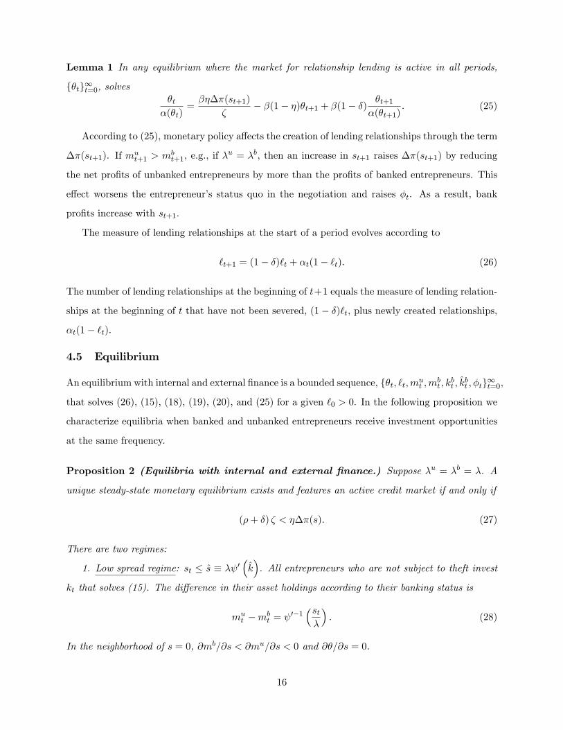
1. Low spread regime: st ≤ s ≡ λψ′(k). All entrepreneurs who are not subject to theft invest

kt that solves (15). The difference in their asset holdings according to their banking status is

mut −mb

t = ψ′−1(stλ

). (28)

In the neighborhood of s = 0, ∂mb/∂s < ∂mu/∂s < 0 and ∂θ/∂s = 0.

16

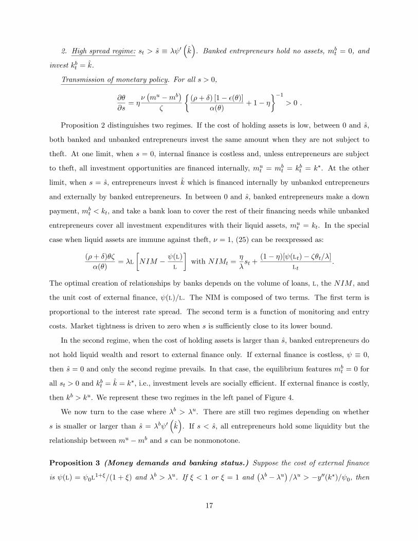
2. High spread regime: st > s ≡ λψ′(k). Banked entrepreneurs hold no assets, mb

t = 0, and

invest kbt = k.

Transmission of monetary policy. For all s > 0,

∂θ

∂s= η

ν(mu −mb

)ζ

(ρ+ δ) [1− ε(θ)]

α(θ)+ 1− η

−1

> 0 .

Proposition 2 distinguishes two regimes. If the cost of holding assets is low, between 0 and s,

both banked and unbanked entrepreneurs invest the same amount when they are not subject to

theft. At one limit, when s = 0, internal finance is costless and, unless entrepreneurs are subject

to theft, all investment opportunities are financed internally, mut = mb

t = kbt = k∗. At the other

limit, when s = s, entrepreneurs invest k which is financed internally by unbanked entrepreneurs

and externally by banked entrepreneurs. In between 0 and s, banked entrepreneurs make a down

payment, mbt < kt, and take a bank loan to cover the rest of their financing needs while unbanked

entrepreneurs cover all investment expenditures with their liquid assets, mut = kt. In the special

case when liquid assets are immune against theft, ν = 1, (25) can be reexpressed as:

(ρ+ δ)θζ

α(θ)= λl

[NIM − ψ(l)

l

]with NIMt =

η

λst +

(1− η)[ψ(lt)− ζθt/λ]

lt.

The optimal creation of relationships by banks depends on the volume of loans, l, the NIM , and

the unit cost of external finance, ψ(l)/l. The NIM is composed of two terms. The first term is

proportional to the interest rate spread. The second term is a function of monitoring and entry

costs. Market tightness is driven to zero when s is suffi ciently close to its lower bound.

In the second regime, when the cost of holding assets is larger than s, banked entrepreneurs do

not hold liquid wealth and resort to external finance only. If external finance is costless, ψ ≡ 0,

then s = 0 and only the second regime prevails. In that case, the equilibrium features mbt = 0 for

all st > 0 and kbt = k = k∗, i.e., investment levels are socially effi cient. If external finance is costly,

then kb > ku. We represent these two regimes in the left panel of Figure 4.

We now turn to the case where λb > λu. There are still two regimes depending on whether

s is smaller or larger than s = λbψ′(k). If s < s, all entrepreneurs hold some liquidity but the

relationship between mu −mb and s can be nonmonotone.

Proposition 3 (Money demands and banking status.) Suppose the cost of external finance

is ψ(l) = ψ0l1+ξ/(1 + ξ) and λb > λu. If ξ < 1 or ξ = 1 and

(λb − λu

)/λu > −y′′(k∗)/ψ0, then

17

bu mm , bu mm ,

uu km = uu km =bm bm

*k *k

k kbk bk

LL L

bu λλ = bu λλ <

Figure 4: Holdings of liquid assets, loan sizes, and investment

there exists 0 < s0 ≤ s1 < +∞ such that: for all s < s0, mb > mu and ∂θ/∂s < 0; for all s > s1,

mu > mb and ∂θ/∂s > 0.

For sake of illustration, suppose the cost of external finance is quadratic, ξ = 1, and ψ0 is

suffi ciently large. When s is low (s < s0), it is optimal for banked entrepreneurs who receive more

frequent investment opportunities to accumulate more liquid assets than unbanked entrepreneurs.

In contrast, if s is large (s > s1), banked entrepreneurs can rely on bank credit to finance investment,

and hence they hold less liquid assets than unbanked entrepreneurs. The crossing of the money

demands, mu (red curve) and mb (blue curve), is illustrated in the right panel of Figure 4. Using

that ∂θ/∂s ∼ mu −mb, the nonmonotonicity of mu −mb with respect to s creates a nonmonotone

relationship between bank entry and spreads. For low spreads, an increase in s reduces bank entry

whereas for high spreads it raises bank entry.

In summary, our model delivers a transmission mechanism from the policy rate to investment

through two channels. There is an internal finance channel whereby an increase in st reduces

entrepreneurs’holdings of liquid assets, which in turn reduces the share of total investment financed

internally. This effect is asymmetric for banked and unbanked entrepreneurs and depends on the

elasticity of ψ(l) and the difference between λb and λu. There is also an external finance channel

according to which an increase in s makes lending relationships more valuable when mu > mb,

which raises bank profits when banks have market power and promotes loan creations.

18

5 Aftermath of a credit shock

We now study the dynamics of the economy following a credit supply shock under alternative

monetary policies. In order to simplify the presentation, we set ν = 1 for now and we reintroduce

ν < 1 when we calibrate the model and turn to the optimal policy analysis. The economy starts at

a steady state with mu0 > mb

0 (which holds if ψ is suffi ciently convex or s is above a threshold) and

`0 = `s. A banking crisis destroys a fraction of the lending relationships, `+0 < `s. We illustrate the

dynamics in a phase diagram for the continuous-time limit of our model (see the Appendix for the

derivations).17

5.1 Interest or liquidity targeting vs. forward guidance

We consider simple policies that illustrate the central trade-offof the policymaker between providing

liquidity to unbanked entrepreneurs and promoting the creation of lending relationships.

Interest rate targeting. The first policy consists in keeping the spread, st, constant over time

so as to maintain an elastic supply of liquidity. The steady state is a saddle point with a unique

saddle path, θt = θs for all t, leading to it, as illustrated by the left panel of Figure 5. For any `0,

the measure of relationships is given by

`t = `s + (`0 − `s) e−[δ+α(θs)]t,

where `s = α(θs)/ [δ + α(θs)]. The speed of recovery, δ + α(θs), increases with the interest rate

spread, s. Aggregate liquidity is given by Mt = `tmb + (1− `t)mu, i.e.,

Mt = Ms + (`s − `0) e−[δ+α(θs)]t(mu −mb),

where Ms = `smb + (1 − `s)mu. Hence, aggregate liquidity jumps upward as the credit shock

occurs, and returns gradually to its steady-state value over time. Investment levels by banked and

unbanked firms are unaffected by the shock, kut = ku0 < kbt = kb0 , as illustrated in the bottom right

panel of Figure 5. Aggregate investment falls since the measure of unbanked firms is higher relative

to the steady state and those firms can only finance a fraction of the investment opportunities of

banked firms (λu < λb).

17For a detailed description of New Monetarist models in continuous time, with methods and applications, see Choiand Rocheteau (2019).

19

l l1 1

0=l 0=l

0=θ

0=θ

>>> > >

> >

0l 0l

Constant spread Constant liquidity supply

0 0

tl

sl

0l

constants

constants

constantM

constantM

tk

utk

btk

uk0

bk0

Figure 5: Transitional dynamics: phase diagram with constant s (top left) and constant M (topright); dynamics of lending relationships (bottom left) and investment (bottom right)

Aggregate liquidity targeting. Suppose next that aggregate liquidity, Mt, is held constant.

The market-clearing spread, s(`,M), is decreasing in both ` and M for all ` and M< k∗ and

s(`,M) = 0 for all M> k∗. The θ-isocline is now downward sloping in (`, θ)-space when M< k∗ and

is horizontal if M> k∗. Intuitively, as ` increases, the aggregate demand for liquid assets decreases,

and hence s decreases, which reduces the profitability of banks and bank entry. The steady state is

a saddle point, and the saddle path is downward sloping if M< k∗, as illustrated by the top right

panel of Figure 5.

If M< k∗, the interest rate spread and credit market tightness increase at the time of the credit

crunch. As the economy recovers, both θ and s decrease and gradually return to their steady-state

values. Investment by banked and unbanked firms drops initially, since s is higher, but recovers

afterwards. So, keeping M constant speeds up the formation of lending relationships (see bottom

left panel of Figure 5), but does not accommodate the higher demand for liquidity created by the

20

larger fraction of unbanked entrepreneurs, thereby reducing individual investment.

Forward guidance. The policymaker faces a trade off between providing liquidity to unbanked

entrepreneurs by keeping spreads low and giving incentives to banks to re-enter and rebuild relation-

ships by raising spreads. In order to address both objectives, the policymaker can take advantage

of banks’dynamic incentives by setting a low interest spread initially, s(t) = sL for all t < T , to

allow unbanked entrepreneurs to self insure at low cost, and by committing to raise the interest

spread at some future date T , i.e., s(t) = sH > sL for all t > T . We illustrate this policy in the top

right panel of Figure 5. The low-spread regime corresponds to a low θ-isocline (θ = θL) and the

high-spread regime corresponds to a high θ-isocline (θ = θH). The arrows of motion characterize

the dynamic system when t < T . The equilibrium path can be obtained by moving backward in

time.18 For all t > T , the economy is on the horizontal saddle path corresponding to s = sH , i.e.,

θt = θH . The path for the economy is continuous at t = T , i.e., θT− = θH , and it reaches the

θH -saddle path by below. Finally, the trajectory of the economy starts at `0 with θ0 > θL. Over

the time interval (0, T ), market tightness rises until it reaches θH at time T . Aggregate liquidity

increases initially due to high demand and low spreads, decreases gradually as `t increases, and

jumps downward when the spread is raised.

5.2 Calibration

We calibrate the model to match moments on U.S. small businesses and their banking relationships.

We use data from the 2003 National Survey of Small Business Finances (SSBF) and Compustat

when the SSBF is insuffi cient. We take the period length as a month and set ρ = (1.04)112 −

1 = 0.0033. We adopt the following functional forms: α (θ) = αθ/(1 + θ), where α ∈ [0, 1],

y (k) = ka/a, and ψ(l) = Bl1+ξ/(1 + ξ), where ξ > 1. The parameters to calibrate are then

(α, δ, ξ, B, a, λu, λb, s, ν, η, ζ).

18Choi and Rocheteau (2019) describe the methodology to solve for equilibria of a continuous-time New Monetaristmodel with policy announcements.

21

Parameter Value Moment Data ModelParameters Set DirectlyDiscount rate (annual %), ρ 4.00Destruction rate, δ 0.01 Avg. length of credit rel. (years) 5.61 5.61Probability of theft, 1− ν 0.0016 Rate of embezzlement and forgery 1.9 1.9

Parameters Set Jointly Moments used in optimizationMatching effi ciency, α 0.093 Share of banked firms 0.68 0.68Production curvature, a 0.555 Elasticity of ctsu to s -0.23 -0.23Productivity shock, unbanked, λu 0.126 Average cash-to-sales, unbanked 0.36 0.36Productivity shock, banked, λb 0.144 Effect of relationship on innovation 1.14 1.14External finance - curvature, ξ 8.604 Elasticity of (ctsu − ctsb) to s 0.07 0.07External finance level, B 6.187 (ctsu − ctsb)/ctsu 0.58 0.58Bargaining power, η 0.522 Average NIM (%) 6.00 6.00Bank entry cost, ζ 0.025 Optimal spread (% annual) 2.00 2.00

We define a credit relationship as an open line of credit or an active business credit card with a

bank. In the 2003 SSBF, 68% of small businesses report being in a credit relationship with a bank,

with an average duration of 8.25 years. We set α = 0.09 and δ = 1/99 to generate ` = 0.68 and an

average length of relationship of 99 months.19

We interpret s as the user cost of holding an index of money-like assets, MSI-ALL, which

includes currency, deposit accounts, and institutional and retail money market funds.20 As our

baseline, we target the optimal long-run spread under commitment to equal the average real user

cost of MSI-ALL from 2002—2004 of 2%. This pins down the fixed cost of bank entry and gives

ζ = 0.025.

We set (λu, a) to target the level and elasticity of cash-to-sales by the unbanked with respect

to the user cost, illustrated in Figure 1. In the model, annual cash-to-sales is given by ctsu =

mu/[12 · λuνy(mu)]. In the data, we rely on evidence from unbanked firms in Compustat since

firms in the SSBF do not consistently report sales for much of the sample.21 This procedure yields

λu = 0.126 and a = 0.56. We then set λb based on the evidence in Cosci et al. (2016) who find

that being in a lending relationship increases the probability of innovation or R&D activity by a

factor of 1.14. Hence, λb = 1.14× λu = 0.144.

19Similarly, Sufi (2009) finds 74.5% of U.S. public, non-financial firms in Compustat have access to lines of creditprovided by banks.20The user cost is the spread between the rate of return of the MSI-ALL index and a benchmark rate equal to the

maximum rate across short-term money market assets plus a liquidity premium of 100 basis points. See Andersonand Jones (2010) for details on constructing the MSI-ALL series and the rate of return and FRED series OCALLP.21Additionally, Compustat delivers a longer time series from 1996 to 2003 versus the shorter variation in the SSBF

from 2003 to 2005 which is important for generating reliable money demand estimates.

22

We set (B, ξ) to target the level and elasticity of the difference in cash-to-sales between unbanked

and banked firms, (ctsu − ctsb), with respect to s. As discussed in Section 2, unbanked small

businesses hold 58% more cash relative to sales. We set B to target (ctsu− ctsb)/ctsu = 0.58 and ξ

to target the elasticity of (ctsu− ctsb) with respect to s of 0.072. This implies (B, ξ) = (6.19, 8.60).

We set ν to match evidence on the incidence of corporate embezzlement and forgery from

the FBI’s Uniform Crime Reporting data. During 2017, 114,110 incidents of embezzlement and

forgery were reported to the FBI.22 The U.S. Census Statistics of U.S. Businesses reports a total

of 5,996,900 employer firms, which implies an annual incidence of 1.9% or a monthly incidence of

0.16%. Hence we set ν = 0.9984.

Finally, we set banks’bargaining power, η, to target the average annual NIM on small business

loans of 6%, as illustrated in right panel of Figure 2.23 This procedure gives η = 0.52.

Response to destruction of relationships. We consider different magnitudes for the size of

the shock: a contraction in ` of 10%, 35%, and 60%. In our calibrated economy, ` falls from

a steady-state of 0.68 to 0.59, 0.43 and 0.26, respectively. These shocks correspond to different

interpretations for the contraction in small business lending in the U.S. during the 2008 banking

crisis and recession.24

Figure 6: Dynamic response to destruction of lending relationships: constant spread (solid) vs.constant liquidity (dashed)

22See https://ucr.fbi.gov/nibrs/2017/tables/data-tables.23Our measure of NIM from (24) is interpreted as the discounted sum of net interest margins over the duration of

the loan. By setting NIM = 6% to its value at an annual frequency, we implicitly interpret the maturity of a loanin the model as a year, thereby aligning it to the frequency of investment opportunities. If the average maturity islonger than a year, the per loan NIM will be higher, and vice versa. To check the sensitivity of our results to thistarget we consider cases in which we either half or double the baseline value of banks’bargaining power, η.24The contraction in lending relationships of 10% is in line with evidence from McCord and Prescott (2014) of a 14%

decline in the number of commercial banks from 2007 to 2013. The larger contractions of 35% and 60% correspondroughly to the fall in the measure of small business loan originations of 40% reported in Chen, Hanson, and Stein(2017) and the fall in the total number of U.S. corporate loans of 60% as reported in Ivashina and Scharfstein (2010).

23

Figure 6 shows the dynamic response of the calibrated model under two fixed monetary policy

rules: the spread s remains constant over time (solid lines) and the aggregate supply of liquidity

M remains constant (dashed lines). Those dynamics are qualitatively similar to those in Figure

5. Quantitatively, the policy that consists in keeping M constant generates a large decline in

aggregate investment (by about 20% under the large shock) which is more than twice as large as

the one obtained under a constant spread. The recovery in terms of lending relationships is faster,

i.e., the half time is reached about 7 months earlier under a constant M than under a constant s.

6 Optimal monetary policy

We now analyze the optimal monetary policy following a credit crisis that destroys a fraction of

lending relationships. In the Appendix, we show any constrained-effi cient allocation has kut = kbt =

k∗, lt = 0, kbt = lt = k. It coincides with a decentralized equilibrium if the policymaker implements

the Friedman rule, st = 0, to achieve optimal investment levels, and the Hosios condition holds,

ε(θt) = η, to guarantee an effi cient creation of lending relationships.25 In the Appendix, we also

establish suffi cient conditions under which the Friedman rule, st = 0 for all t, is suboptimal. If

the difference between ε(θ) and η is suffi ciently large relative to 1/ξ, increasing st+1 above 0 raises

the creation of relationships which is ineffi ciently low in the decentralized equilibrium, and the

associated welfare gain outweighs the monitoring cost of bank loans.26

6.1 The Ramsey problem

Suppose the policymaker chooses an infinite sequence of interest spreads to implement a decen-

tralized equilibrium that maximizes social welfare. The policy path, st∞t=1, is announced before

the market for relationships opens in stage 2, and the policymaker commits to it.27 We write the

Ramsey problem recursively by treating credit market tightness in every period t ≥ 1, θt, as a state

variable. The initial tightness, θ0, is chosen to place the economy on the optimal path. Market

tightness, θt, is interpreted as a promise to banks that determines their future profits. It must be

honored in period t + 1 by choosing st+1 and θt+1 consistent with the free entry condition, (25).

25See the appendix for a formal proof. For a related result, see Berentsen, Rocheteau, and Shi (2007).26We do not allow the policymaker to make direct transfers to banks that participate in the credit market in order

to correct for ineffi ciently low entry. Such transfers may not be feasible if the policymaker cannot distinguish betweenactive and inactive banks in the credit market (i.e., one could create a bank but not search actively in the creditmarket).27We also consider commitment under a timeless approach based on Woodford (1999, 2003) in the Appendix.

24

The recursive planner’s problem is

W(`t, θt) = maxθt+1∈Γ(θt)

−ζθt(1− `t) + β(1− `t+1)λuν

[y(mu

t+1)−mut+1

](29)

+β`t+1λbν[y(kbt+1

)− kbt+1 − ψ(lt+1)

]+ (1− ν)

[y(k)− k − ψ(k)

]+ βW(`t+1, θt+1)

,

where Γ(θt) is the set of values for θt+1 consistent with (25) for some st+1 ∈ [0,+∞). Given st+1,

the quantities mut+1, k

bt+1, and lt+1 are obtained from (15) and (19).28 The policymaker’s problem

at the beginning of time is

W(`0) = maxθ0∈Ω=[θ,θ]

W(`0, θ0), (30)

where θ (respectively, θ) is the steady-state value of θ if s = 0 (respectively, s =∞).

Figure 7: Optimal policy response with commitment to a destruction of lending relationships

Figure 7 illustrates the optimal policy response following a banking shock that destroys lending

relationships in the calibrated economy. The Ramsey solution lowers st close to the lower bound at

the onset of the crisis and then raises it above its long-run value (forward guidance) before gradually

decreasing it to the stationary level. The hump-shaped path of the optimal spread (top left panel

of Figure 7) causes a similar hump-shaped response in credit market tightness (top middle panel).

While low spreads benefit unbanked firms by making internal finance less costly, they dampen bank

28The existence and uniqueness of W(`, θ) is established in the Appendix.

25

profits and reduce the incentives to create new relationships. The use of forward guidance mitigates

the effect of the current spread on relationship creation because banks’lifetime profits depend on

the whole path of future spreads. For smaller shocks, initial spreads are lower for longer and only

gradually increase over time. However, for large shocks, spreads increase more rapidly and feature

a more pronounced hump-shaped response.

Low spreads induce all firms to raise their holdings of liquid assets closer to the full insurance

level k∗ = 1 (bottom middle). Over time, the policymaker gradually unwinds the initial expansion

of M, leading to a sharp decline in banked firms’cash holdings relative to unbanked firms. Initially,

the increase in liquidity goes beyond what is necessary to keep aggregate investment constant (top

right). Afterwards, aggregate investment falls and reaches its lowest value after about 16 months.

It recovers gradually as it increases towards its long-run value.

6.2 Optimal policy without commitment

We now relax the assumption of commitment altogether and assume the policymaker sets st+1

in period t but cannot commit to st′t′>t+1.29 As in Klein, Krusell, and Rios-Rull (2008), the

policymaker moves first by choosing st+1, and the private sector moves next by choosing θt+1,

mut+1, and m

bt+1.

We restrict our attention to Markov perfect equilibria. The policymaker’s strategy consists of

a spread st+1 at the beginning of stage 2 of period t as a function of the economy’s state, `t. From

(15), mut = y′−1 [1 + st/λ

u], so the strategy of the policymaker can be represented bymut+1 = K (`t).

The strategy of banks to enter is expressed as θt = Θ(`t,mut+1), where Θ is implicitly defined by

(25), i.e.,

Θ(`t,mut+1)

α[Θ(`t,mu

t+1)] =

βη∆π(mut+1)

ζ− β(1− η)Θ(`t+1,m

ut+2) + β(1− δ)

Θ(`t+1,mut+2)

α[Θ(`t+1,mu

t+2)] , (31)

where `t+1 = (1− δ)`t + α[Θ(`t,m

ut+1)

](1− `t) and mu

t+2 = K (`t+1). When forming expectations

about θt+1, banks anticipate the policymaker in period t+ 1 will adhere to his policy rule, mut+2 =

K (`t+1), and hence θt+1 = Θ [`t+1,K (`t+1)]. In equilibrium, θt = Θ(`t,mut+1) and mu

t+1 = K (`t)

are best responses to each other.

29As an alternative to relaxing the commitment assumption altogether, we consider in the Appendix the timelessapproach to the Ramsey problem as in Woodford (2003).

26

Given Θ, we determine K (`t) recursively from:

W(`t) = maxmut+1∈[0,k∗]

−ζ(1− `t)Θ

(`t,m

ut+1

)+ β(1− `t+1)λuν

[y(mu

t+1)−mut+1

](32)

+β`t+1λbν[y(kbt+1

)− kbt+1 − ψ(lt+1)

]+ (1− ν)

[y(k)− k − ψ(k)

]+βW (`t+1) , (33)

where kbt+1 and lt+1 can be expressed as functions of mut+1. The entire transitional dynamics are

computed numerically by devising a two-dimensional iteration described in the Appendix. Figure

8 illustrates the optimal policy response under the benchmark calibration.

Figure 8: Optimal policy response without commitment to a destruction of lending relationships

The policymaker can no longer commit to raise future st to counteract the effects of current st

on banks’lifetime expected profits, as in the Ramsey problem. In the long run, it is optimal to set

spreads at their lower bound, zero, which illustrates the bias of the policymaker toward low interest

rates. When the shock to banking relationships is small, the optimal policy is to keep spreads

unchanged at their optimal long-run level (top left panel of Figure 8). However, for large enough

shocks, the policymaker raises spreads at the outset of the credit crunch when `t is low in order to

rebuild relationships more quickly. As lending relationships recover, st is reduced gradually over

time. Quantitatively, interest spreads early on are larger than the ones from the Ramsey solution

when the shock is large enough, but future spreads are lower.

27

There are two effects on aggregate liquidity at the onset of the crisis. The increase in spreads

lowers holdings of liquid assets for all firms, thereby decreasing Mt. However the fall in ` from

the credit shock increases Mt since mu > mb. Quantitatively, the second effect tends to dominate

(bottom right). In contrast to the Ramsey solution, aggregate investment falls at the time of the

shock and recovers gradually (top right).

In our calibrated example, the half life of the recovery following a 60% contraction is 20 months

under the Ramsey solution but 27 months under the no commitment policy. So, the inability to

commit slows down the recovery by about 7 months. The welfare loss from the lack of commitment

ranges from 0.90% to 0.98% of foregone output, depending on the size of the shock.30 These esti-

mates are consistent with those in Klein, Krussell, and Rios-Rull (2008) who study time consistent

capital income taxation and find that without commitment, steady-state consumption is about

0.5% lower relative to the commitment case.

6.3 Optimal Policy following a temporary lockdown

We conclude this section on optimal monetary policy by analyzing the response to an unanticipated,

but temporary, business lock-down. The shock aims to capture the COVID-19 pandemic that has

forced a large fraction of small businesses to shut down operations. Our model is able to speak to an

aspect of the crisis where large disruptions in firms’production reduces the incentive for banks to

create new lending relationships while existing relationships are destroyed at a constant rate, with

potential consequences for the recovery. To capture the temporary lock-down, we assume the rates

of production opportunities, λu and λb, unexpectedly fall by 40%, based on a recent report (U.S.

Chamber of Commerce 2020) that 25% to 55% of small businesses either closed or would likely

close as a result of COVID-19.31 We consider three scenarios where the lock-down lasts three, six,

or twelve months, then returns to its normal, pre-pandemic levels.

Figure 9 plots the optimal response when the policy maker has commitment. The top left panel

illustrates the disruption in production opportunities faced by the unbanked (the disruption faced

by the banked looks similar). If the disruption is anticipated to last three months (green lines), the

response consists of initially lowering st close to the lower bound (top middle panel) and keeping

30We measure the welfare cost of not implementing the Ramsey solution as 1 − Wp/WR, where WR is lifetimediscounted output under the Ramsey policy and Wp is lifetime discounted output under the optimal policy with nocommitment. In the Appendix, we report robustness checks on various parameters (e.g., ν) and summarize how thiswelfare cost is affected.31Similarly, Bartik et al. (2020) surveyed small businesses and found 43% of them were temporarily closed.

28

the spread low past when the shock is over, only gradually returning to normal after around 20

months. Despite low spreads, θt falls initially but begins to rise before the shock is over. Banks

anticipate that production activity will return to normal and therefore have incentives to create

long lasting relationships before the recovery materializes. Aggregate investment (bottom right)

overshoots its long-run level upon recovery.

Figure 9: Optimal policy response to a temporary reduction in λu and λb by 40%

When the length of the disruption becomes longer at six or twelve months (dashed blue and

dotted red lines in Figure 9) optimal policy still features low initial spreads, but the policymaker

increases spreads gradually before the lock-down is over and increases them discontinuously at the

time of the recovery, above their long-run value. High future spreads prevent tightness and the

measure of lending relationships from falling too low. As a result, aggregate investment (bottom

left) returns to normal levels as soon as the lock-down ends.

7 Conclusion

In this paper, we argue that the formation of lending relationships is critical for small businesses to

finance their investment opportunities. As the formation of these relationships can be influenced

by monetary policy, we developed a general equilibrium model of corporate finance that formalizes

this transmission mechanism, building on recent theories of money demand under idiosyncratic risk

29

and financial intermediation in over-the-counter markets. We use our model to study the optimal

response of the monetary authority following a banking crisis described as an exogenous destruction

of a fraction of the existing lending relationships. We consider different assumptions regarding the

policymaker’s power to commit to setting a time path of interest spreads.

If the policymaker can commit over an infinite time horizon, the optimal policy involves "forward

guidance": the interest spread is set close to its lower bound at the outset of the crisis and increases

over time as the economy recovers. It is this promise of high future spreads that provides banks

incentives to keep creating lending relationships, even in a low spread environment. However, such

promises are not time consistent. If the policymaker cannot commit more than one period ahead,

then the interest rate spread is persistently low and the recession is more prolonged.

Our model of lending relationships and corporate finance can be extended in several ways. For

instance, one could relax the assumption that banks can fully enforce repayment to study imperfect

pledgability of firms’returns and its relation with monetary policy (e.g., as in Rocheteau, Wright,

and Zhang 2018). In addition, while we assume full commitment by banks, one could consider

banks’ limited commitment and analyze the dynamic contracting problem in the credit market

(e.g., as in Bethune, Hu, and Rocheteau 2017) or agency problems between firms and banks to

capture additional benefits of lending relationships (e.g., Hachem 2011, Boualam 2017). It would

be fruitful to develop a life-cycle version of our model to explain firms’cash accumulation patterns

and their interaction with long term credit lines. Finally, our model of relationship lending could

be applied in other institutional contexts, like the interbank market (Brauning and Fecht 2016).

30

References

Adams, Robert and Jacob Gramlich (2014). Where are all the New Banks? The Role ofRegulatory Burden in New Bank Formation, Finance and Economics Discussion Series 113.Anderson, Richard and Barry Jones (2011). A Comprehensive Revision of the US MonetaryServices (Divisia) Indexes, Federal Reserve Bank of St. Louis Review, 93(5), 235-259.Agarwal, Sumit and Robert Hauswald (2010). Distance and Private Information in Lending,Review of Financial Studies, 23, 2757-2788.Alvarez, Fernando and Urban Jermann (2000). Effi ciency, Equilibrium, and Asset Pricingwith Risk of Default , Econometrica, 68, 776-797.Aruoba, Boragan and Sanjay Chugh (2010). Optimal Fiscal and Monetary Policy WhenMoney is Essential. Journal of Economic Theory , 145, 1618-1647.Atkeson, Andrew, Andrea Eisfeldt, and Pierre-Oliver Weill (2015). Entry and Exit inOTC Derivative Market. Econometrica, 83(6), 2231-2292.Azar, Jose, Jean-Francois Kagy, and Martin Schmalz (2016). Can Changes in the Cost ofCarry Explain the Dynamics of Corporate Cash Holdings? Review of Financial Studies 8, 2194-2240.Balloch, Cynthia and Yann Koby (2020). Low Rates and Bank Low Supply: Theory andEvidence From Japan. Working Paper.Barnett, William (1980). Economic Monetary Aggregates an Application of Index NumberTheory and Aggregation Theory, Journal of Econometrics, 14(1), 11—48.Bartik, Alexander, Marianne Bertrand, Zoe Cullen, Edward Glaeser, Michael Luca,and Christopher Stanton (2020). How Are Small Businesses Adjusting to COVID-19? EarlyEvidence from a Survey. Becker Friedman Institute Working Paper No. 2020-42.Barro, Robert and David Gordon (1983). A Positive Theory of Monetary Policy in a NaturalRate Model. Journal of Political Economy, 91 (4): 589-610.Berger, Allen and Gregory Udell (1995). Small Firms, Commercial Lines of Credit, andCollateral. Journal of Business, 68(3): 351-382.Berlin, Mitchell and Loretta Mester (1999). Deposits and Relationship Lending. Review ofFinancial Studies, 12, 579.Berry, Jared, Felicia Ionescu, Robert Kurtzman, and Rebecca Zarutskie (2019). Changesin Monetary Policy and Banks’ Net Interest Margins: A Comparison Across Four TighteningEpisodes, FEDS Notes.Bethune, Zachary, Tai-We Hu, and Guillaume Rocheteau (2017). Optimal Credit Fluctu-ations. Review of Economic Dynamics, forthcoming.Berentsen, Aleksander, Guillaume Rocheteau, and Shouyong Shi (2007). Friedman MeetsHosios: Effi ciency in Search Models of Money. Economic Journal, 117, 174-195.Bolton, Patrick and Xavier Freixas (2006). Corporate Finance and the Monetary PolicyTransmission Mechanism. The Review of Financial Studies, 19(3), 829-870.Bolton, Patrick, Xavier Freixas, Leonardo Gambacorta, and Paolo Emilio Mistrulli(2016). Relationship Lending and Transaction Lending in a Crisis. The Review of FinancialStudies, 29(10).Boualam, Yasser (2017). Bank Lending and Relationship Capital. Mimeo.Borio, Claudio, Leonardo Gambacorta, and Boris Hofmann (2017). The Influence ofMonetary Policy on Bank Profitability. International Finance, 20(1),Brauning, Falk and Falko Fecht (2016). Relationship Lending in the Interbank Market andthe Price of Liquidity. Boston Fed Working Paper.Chang, Roberto (1998). Credible Monetary Policy in an Infinite Horizon Model: RecursiveApproaches. Journal of Economic Theory, 81, 431-461.

31

Chen, Brian, Samuel Hanson, and Jeremy Stein (2017). The Decline of Big Bank Lendingto Small Businesses: Dynamic Impacts of Local Credit and Labor Markets. Mimeo.Choi, Michael and Guillaume Rocheteau (2019). New Monetarism in Continuous Time:Methods and Applications. Economic Journal, Forthcoming.Claessens, Stijn, Nicholas Coleman, and Michael Donnelly (2018). “Low for Long”Inter-est Rates and Banks’Interest Margins and Profitability: Cross-Country Evidence. InternationalFinance Discussion Papers 1197.Cohen, Jon, Kinda Cheryl Hachem, and Gary Richardson (2016). Relationship Lendingand the Great Depression: New Measurement and Implications. NBER Working Paper No. 22891.Corbae, Dean and Joseph Ritter (2004). Decentralized Credit and Monetary Exchange withoutPublic Record Keeping. Economic Theory, 24, 933-951.Cosci, Stefania, Valentina Meliciani, and Valentina Sabato (2016). Relationship lendingand innovation: Empirical evidence on a sample of European firms. Economics of Innovation andNew Technology, 25(4), 335-357.den Haan, Wouter, Garey Ramey, and Joel Watson (2003). Liquidity Flows and Fragilityof Business Enterprises. Journal of Monetary Economics, 50, 1215-1241.Diamond, Douglas (1984) . Financial Intermediation and Delegated Monitoring. Review of Eco-nomic Studies, 393-414.Diamond, Douglas (1991) . Monitoring and Reputation: the Choice Between Bank Loans andDirectly Placed Debt. Journal of Political Economy, 99(4).Duffi e, Darrell, Garleanu, Nicolae, and Pedersen, Lasse (2005). Over-the-Counter Markets.Econometrica, 73, 1815-47.Dreschler, Itamar, Alexi Savov, and Philipp Schnabl (2017). The Deposits Channel ofMonetary Policy. Quarterly Journal of Economics, forthcoming.Ennis, Huberto, Helen Fessenden, and John Walter (2016). Do Net Interest Margins andInterest Rates Move Together? FRB Richmond Economic Brief.Elyasiani, Elyas and Lawrence Goldberg (2004). Relationship Lending: A Survey of theLiterature. Journal of Economics and Business, 56, 315-330.Graham, John and Mark Leary (2018). The Evolution of Corporate Cash. Review of FinancialStudies, 31(11), 4288-4344.Grochulksi, Borys, Daniel Schwam, and Yuzhe Zhang (2018). Cyclical Properties of BankMargins: Small Versus Large Banks, Economic Quarterly, 1-33.Gu, Chao, Mattesini, Fabrizio, Monnet, Cyril and Wright, Randall (2013). Banking: ANew Monetarist Approach. Review of Economic Studies, 80, 636-66.Gu, Chao, Fabrizio Mattesini, and Randall Wright (2016). Money and Credit Redux.Econometrica, 84(1), 1-32.Hachem, Kinda Cheryl (2011). Relationship Lending and the Transmission of Monetary Policy.Journal of Monetary Economics, 58, 590-600.He, Ping, lixin Huang and Randall Wright (2005). Money and Banking in Search Equilibrium.International Economic Review, 46(2), 637-670.Hendershott, Terrence, Dan Li, Dmitry Livdan, and Normal Schurhoff (2017) . Rela-tionship Trading in OTC Markets. Mimeo.Herrera, Ana Maria, and Raoul Minetti (2007). “Informed Finance and TechnologicalChange: Evidence from Credit Relationships.” Journal of Financial Economics, 83(1): 223-269.Holmstrom, Bengt, and Jean Tirole (1997). Financial Intermediation, Loanable Funds andthe Real Sector. Quarterly Journal of Economics, 112, 663.Huang, Rocco (2009). How Committed Are Bank Lines of Credit? Evidence from the SubprimeMortgage Crisis. Working Paper.Imhof, Stephan, Cyril Monnet, and Shenxing Zhang (2018). The Risk-Taking Channel ofLiquidity Regulations and Monetary Policy. Mimeo.

32

Ivashina, Victoria and David Scharfstein (2010). Bank Lending During the Financial Crisisof 2008. Journal of Financial Economics, 97, 319-338.Kehoe, Timothy and David Levine (1993). Debt-Constrained Asset Markets. Review ofEconomic Studies, 60, 865-888.Kiyotaki, Nobuhiro and John Moore (2005). Liquidity and Asset Prices. International Eco-nomic Review, 46, 317-49.Klein, Paul, Per Krusell, Jose-Victor Rios-Rull (2008). Time-Consistent Public Policy.Review of Economic Studies, 75, 789-808.Lagos, Ricardo (2010). Asset Prices and Liquidity in an Exchange EconomyJournal of EconomicTheory, 57(8), 913-930.Lagos, Ricardo and Guillaume Rocheteau (2009). Liquidity in Asset Markets with SearchFrictions, Econometrica, 77(2), 403-426.Lagos, Ricardo Guillaume Rocheteau and Pierre Oliver Weill (2011). Crises and Liquidityin Over-the-Counter Markets. Journal of Economic Theory, 146, 2169-2205.Lagos, Ricardo Guillaume Rocheteau and Randall Wright (2017). Liquidity: A NewMonetarist Perspective. Journal of Economic Literature, forthcoming.Lagos, Ricardo and Wright, Randall (2005). A Unified Framework for Monetary Theory andPolicy Analysis. Journal of Political Economy, 113, 463-484.Lester, Benjamin, Andrew Postlewaite, and Randall Wright (2012) . Information, Liquid-ity, Asset Prices, and Monetary Policy. Review of Economic Studies, 79 (3), 1208-1238.Li, Yiting, Guillaume Rocheteau, and Pierre-Olivier Weill (2012). Liquidity and theThreat of Fraudulent Assets. Jounal of Political Economy, 120, 815-846.Martin, Fernando (2011) . On the Joint Determination of Fiscal and Monetary Policy. Journalof Monetary Economics, 58(2), 132-145.Martin, Fernando (2013) . Government Policy in Monetary Economies. International EconomicReview, 54(1), 185-217.McCord, Roisin and Edward S. Prescott (2014) . The Financial Crisis, the Collapse of BankEntry, and Changes in the Size Distribution of Banks. Economic Quarterly, 100(1), 23-50.Mulligan, Casey (1997). Scale Economies, the Value of Time, and the Demand for Money:Longitudinal Evidence from Firms, Journal of Political Economy, 105(5), 1061—1079.Petersen, Mitchell and Raghuram Rajan (1994). The Benefits of Lending Relationships:Evidence from Small Business Data. Journal of Finance, 49, 3-37.Petrosky-Nadeau, Nicolas and Etienne Wasmer (2017). Labor, Credit, and Goods Markets,MIT Press.Pissarides, Christopher (2000). Equilibrium Unemployment, MIT Press.Rajan, Raghuram (1992). Insiders and Outsiders: The Choice Between Informed Investors andArm’s Length Debt. Journal of Finance, 47, 1367.Raveendranathan, Gajendran (2020). Revolving Credit Lines and Targeted Search. Mimeo.Rocheteau, Guillaume and Ed Nosal (2017). Money, Payments, and Liquidity. MIT Press.Rocheteau, Guillaume and Antonio Rodriguez-Lopez (2014). Liquidity Provision, InterestRates, and Unemployment. Journal of Monetary Economics, 65, 80-101.Rocheteau, Guillaume and Randall Wright (2005) . Money in Search Equilibrium, in Com-petitive Equilibrium, and in Competitive Search Equilibrium. Econometrica, 73(1), 175-202.Rocheteau, Guillaume, Randall Wright, and Sylvia Xiao (2018). Open Market Operations.Journal of Monetary Economics, forthcoming.Rocheteau, Guillaume, Tsz-Nga Wong, and Cathy Zhang (2018). Lending Relationshipsand Optimal Monetary Policy. Mimeo.Rocheteau, Guillaume, Randall Wright, and Cathy Zhang (2018). Corporate Finance andMonetary Policy. American Economic Review, 108(4-5), 1147-1186.

33

Sanches, Daniel and Stephen Williamson (2010). Money and Credit with Limited Commit-ment and Theft. Journal of Economic Theory, 145, 1525-1549.Sanchez, Juan and Emircan Yurdigal (2013). Why Are U.S. Firms Holding So Much Cash?An Exploration of Cross-Sectional Variation. FRB St. Louis Review, 95(4), 293-325.Sharpe, Steven (2014). Asymmetric Information, Bank Lending, and Implicit Contracts: AStylized Model of Customer Relationships. Journal of Finance, 45(4), 1069-1087.Stokey, Nancy and Robert Lucas (1989). Recursive Methods in Economic Dynamics, HarvardUniversity Press.Sufi, Amir (2009). Bank Lines of Credit in Corporate Finance: An Empirical Analysis. Reviewof Financial Studies, 22, 1057-1088.U.S. Chamber of Commerce (2020). MetLife and U.S. Chamber of Commerce Special Reporton Coronavirus and Small Businesses, April 3, 2020.Wasmer, Etienne and Phillipe Weil (2004). The Macroeconomics of Labor and Credit MarketFrictions. American Economic Review, 94, 944-963.Weill, Pierre-Olivier (2007) . Leaning Against the Wind. Review of Economic Studies, 74, 1329-1354.Williamson, Stephen (2002) . Private Money and Counterfeiting. FRB Richmond EconomicQuarterly, , 88, 37-58.Williamson, Stephen (2012) . Liquidity, Monetary Policy, and the Financial Crisis: A NewMonetarist Approach. American Economic Review, 102, 2570-2605.Woodford, Michael (1999) . How Should Monetary Policy Be Conducted in an Era of PriceStability? in New Challenges for Monetary Policy: Kansas City, FRB Kansas City.Woodford, Michael (2003) . Interest and Prices: Foundations of a Theory of Monetary Policy,Princeton University Press.

34

Appendix A1: Proofs of Propositions and Lemmas

Proof of Proposition 1. We first compute the surplus of being in a lending relationship forentrepreneurs and banks. Recall from (4) and (5) that the lifetime expected utilities of banked andunbanked entrepreneurs with wealth ω in the last stage of period t solve:

W et (ω) = ω −

mut+1

1 + rt+1+ βU et+1(mu

t+1), (34)

Xet (ω) = ω −

mbt+1

1 + rt+1+ βZet+1(mb

t+1). (35)

The surplus of a banked entrepreneur is defined as Set =[Xet−1(0)−W e

t−1(0)]/β. Substituting Zet

by its expression given by (11), i.e.,

Zet (mbt) = νmb

t − φt + λbν[y(kbt )− kbt

]+ λb(1− ν)

[y(kbt )− kbt

]+ δW e

t (0) + (1− δ)Xet (0),

into (35) and subtracting W et−1(0), we obtain:

βSet = β−νstmb

t − φt + λbν[y(kbt )− kbt

]+ λb(1− ν)

[y(kbt )− kbt

]+(1− δ)β [Xe

t (0)−W et (0)] + βW e

t (0)−W et−1(0). (36)

From (9), for all mut ≤ k∗,

U et (mut ) = λuν [y(mu

t )−mut ] + νmu

t + V et (0),

which we substitute into (34) to express W et−1(0) as:

W et−1(0) = β−νstmu

t + λuν [y(mut )−mu

t ]+ βV et (0).

Substituting W et−1(0) into (36) and dividing both sides by β we obtain:

Set = −φt − νstmbt + λbν

[y(kbt )− kbt

]+ λb(1− ν)

[y(kbt )− kbt

](37)

− [πut + V et (0)−W e

t (0)] + (1− δ)βSet+1.

From (12), the surplus of the bank solves

Sbt = φt − λbνψ(kbt −mb

t

)− λb(1− ν)ψ

(kbt

)+ β(1− δ)Sbt+1, (38)

where mbt is the entrepreneur’s down payment on the loan and hence lt = kbt −mb

t is the loan size.Summing (37) and (38), the total surplus of a lending relationship, St = Set + Sbt , solves

St = −νstmbt + λbν

[y(kbt )− kbt − ψ

(kbt −mb

t

)](39)

+λb(1− ν)[y(kbt )− kbt − ψ

(kbt

)]− [πut + V e

t (0)−W et (0)] + (1− δ)βSt+1.

A lending relationship contract negotiated at time t− 1 is

kbt+τ , kbt+τ ,mbt+τ , φt+τ∞τ=0 ∈ arg max[Sbt ]η[Set ]1−η. (40)

35

Given the linearity of Set and Sbt in φt, a solution is such that kbt+τ , kbt+τ ,mbt+τ∞τ=0 ∈ arg max

Sbt + Set

and φt ∈ arg max[Sbt ]η[Set ]1−η. The maximization of the total surplus implies kbt = k such that

y′(k) = 1 + ψ′(k). Maximizing St with respect to kbt and mb

t gives:

y′(kbt )− 1− ψ′(kbt −mb

t

)= 0

−νst + λbνψ′(kbt −mb

t

)≤ 0, “=”if mb

t > 0.

The sequence of intermediation fees solves Sbt+τ = ηSt+τ for all τ , where Sbt obeys (38). Using thedefinition of πb(st) in (21) we can reexpress St as:

St = πb(st)− πu(st)− [V et (0)−W e

t (0)] + (1− δ)βSt+1. (41)

Solving for φt gives

φt = λbνψ(kbt −mb

t

)+ λb(1− ν)ψ

(k)

+ η[πb(st)− πu(st)

]− η [V e

t (0)−W et (0)] .

Using that from (6), V et (0) = αtX

et (0)+(1−αt)W e

t (0), it follows that V et (0)−W e

t (0) = αt [Xet (0)−W e

t (0)] =βαtSet+1. From the bargaining, Set+1 = (1 − η)Sbt+1/η and from the free-entry condition in (7),Sbt+1 = ζθt/(βαt). Putting all this together, we obtain (20).

Proof of Lemma 1. From (6), V et (0) −W e

t (0) = αtβSet+1 = αt(1 − η)βSt+1 where we usedthe generalized Nash solution, i.e. Set+1 = (1− η)St+1. Substituting into (41) to obtain:

St = ∆π(st)− αt(1− η)βSt+1 + (1− δ)βSt+1. (42)

The first two terms on the right side of (42), ∆π(st) − αt(1 − η)βSt+1, represent the flow surplusfrom a lending relationship: it is the increase in the expected profits of the entrepreneur from havingaccess to external finance net of the entrepreneur’s outside option. From (7), assuming positiveentry in equilibrium, V b

t = V bt+1 = 0 implies ζθt = αtηβSt+1. Substituting St+1 = ζθt/ (ηβαt) into

(42) gives (25).

Proof of Proposition 2. From (25) with θt = θt+1 = θ, steady-state credit market tightnessis the unique solution to

(ρ+ δ)θ

α(θ)+ (1− η)θ =

η[πb (s)− πu (s)

]ζ

. (43)

Using that the left side is increasing in θ and limθ→0 θ/α(θ) = 1, (43) admits a positive solution if

(ρ+ δ) ζ < η[πb (s)− πu (s)

].

By differentiating (43) and using that πb′ (s) = −νmb and πu′ (s) = −νmu we obtain:

∂θ

∂s= η

ν(mu −mb

)ζ

(ρ+ δ)

[1− ε(θ)]α(θ)

+ (1− η)

−1

. (44)

From (15) and (19), if λb = λu = λ, then mu > mb for all s > 0. Hence, from the expression above,∂θ/∂s > 0 for all s > 0.

36

Given θ, closed-form solutions for (`,mu,mb, kb, φ) are obtained recursively as follows:

` =α(θ)

δ + α(θ)(45)

s

λ= y′(mu)− 1 (46)

mb = maxmu − ψ′−1

( sλ

), 0

(47)

kb = maxmu, k

(48)

φ = λ(1− ν)ψ(k) + λνψ(kb −mb) + η[πb(s)− πu(s)

]− (1− η)ζθ. (49)

Equation (45) is obtained from (26). Equation (46) corresponds to (15). Equation (47) correspondsto (19) where we used that if mb > 0 then kb = ku = mu and hence ψ′

(kb −mb

)= s/λ. By taking

the inverse of ψ′, mb = mu − ψ′−1 (s/λ). If mb = 0, then y′(kb)− 1 = ψ′(kb)≤ s/λ = y′(mu)− 1.

It follows that mu ≤ kb ≤ ψ′−1 (s/λ) where kb = k. This gives (48). Finally, (49) is obtained from(20).

The low-spread regime corresponds to the case where the constraint mb ≥ 0 does not bind.Hence kb = ku = mu and mb = mu −ψ′−1 (s/λ), which corresponds to (28). The condition mb ≥ 0for all s such that mu ≥ ψ′−1 (s/λ), i.e., y′−1 (1 + s/λ) ≥ ψ′−1 (s/λ). The left side is decreasingin s while the right side is increasing in s, so there is a threshold s such that the inequality holds

for all s ≤ s. The threshold solves y′−1 (1 + s/λ) = ψ′−1 (s/λ), i.e., y′(k) − 1 = ψ′(k)

= s/λ.

The high-spread regime corresponds to the case where the constraint mb ≥ 0 binds, in which casekb = k and s > s.

Finally, in the neighborhood of s = 0, from (46) and (47),mu = mb ≈ k∗. From (44), ∂θ/∂s ≈ 0.Differentiating (46) and (47),

∂mb

∂s=

1

λy′′(k∗)− 1

λψ′′(0)<∂mu

∂s=

1

λy′′(k∗)< 0.

Proof of Proposition 3. From (15) and (19), mb and mu are continous functions of s suchthat mb = mu = k∗ when s = 0. If ∂

(mb −mu

)/∂s > 0 when evaluated at s = 0+ then there

exists s0 > 0 such that mb > mu for all s < s0. By differentiating the FOC (19),

∂mb

∂s=

1

y′′(kb)λb− 1

ψ′′(kb −mb)λb.

Using that ψ′′(kb −mb) = ψ0(kb −mb)ξ−1/ξ, in the neighborhood of s = 0+,

∂mb

∂s=

1

y′′(k∗)λb1

y′′(k∗)λb− 1

ψ0λb

−∞if ξ

< 1= 1> 1.

The condition ∂mb/∂s > ∂mu/∂s = 1/ [y′′(k∗)λu] holds if ξ < 1; it is equivalent to

λb − λu

λu>−y′′(k∗)ψ0

37

if ξ = 1; it does not hold if ξ > 1. Hence, if ξ < 1 or ξ = 1 and(λb − λu

)/λu > −y′′(k∗)/ψ0,

then there exists s0 > 0 such that mb > mu for all s < s0. By the same reasoning as in the

proof of Proposition 2, for all s > λbψ′(k), mb = 0 < mu. The effect of a change in s on market

tightness is obtained from (44) in the proof of Proposition 2, according to which ∂θ/∂s ∼ ∆π′(s) =ν(mu −mb

).

Proposition 4 (Implementing constrained effi cient allocations.) The equilibrium achievesthe constrained-effi cient allocation if and only if st = 0 and ε(θt) = η for all t.

Proof of Proposition 4. We measure social welfare starting in stage 2 of period 0 as the dis-counted sum of aggregate output flows net of the costs associated with production, intermediation,and bank entry: W(`0) =

∑∞t=0 β

tWt where the period welfare is

Wt = −ζθt(1− `t) + β(1− `t+1)λuν[y(kut+1

)− kut+1

](50)

+β`t+1λbν[y(kbt+1)− kbt+1 − ψ (lt+1)

]+ (1− ν)

[y(kbt+1)− kbt+1 − ψ (lt+1)

].

The first term on the right side of (50) are banks’entry costs in the relationship lending market;the second term represents the profits of unbanked entrepreneurs; and the third term representsthe profits of banked entrepreneurs net of the costs of external finance. The planner choosesθt, k

ut+1, k

bt+1, k

bt+1, lt+1, lt+1

∞t=0

to maximize W(`0) subject to the constraint imposed by the

matching technology, α(θt), and the financial constraint according to which the investment ofentrepreneurs who are victims of theft must be financed with bank loans, kbt+1 ≤lt+1.

From the maximization of (50) with respect to (kut+1, kbt+1, k

bt+1,lt+1,lt+1), any constrained-

effi cient allocations satisfy:

kut+1 = kbt+1 = k∗ (51)

lt+1 = 0 (52)

kbt+1 = lt+1 = k. (53)

According to (51), the planner chooses the first-best level of investment, k∗, to maximize profitswhenever it is not subject to the bank financing constraint. In that case, from (52), the loan sizeis zero. From (53), whenever a bank loan is the only option to finance an investment opportunity,then the optimal investment is k = arg max [y(k)− k − ψ (k)]. The comparison of the equilibriumconditions (15) and (19) with (51) shows that a necessary condition for the implementation of aconstrained-effi cient allocation is st+1 = 0 for all t.

Using (51)-(53), we write the planner’s problem recursively as

W(`t) = maxθt≥0−ζθt(1− `t) + β(1− `t+1)λuν [y (k∗)− k∗] (54)

+β`t+1λbν [y(k∗)− k∗] + (1− ν)

[y(k)− k − ψ

(k)]

+ βW(`t+1),

where `t+1 = (1 − δ)`t + α(θt)(1 − `t). Assuming an interior solution, the planner’s optimalityconditions are:

ζ = α′(θt)βωt (55)

ωt =(λb − λu

)ν [y(k∗)− k∗] + λb(1− ν)

[y(k)− k − ψ

(k)]

(56)

+β 1− δ − α(θt+1) [1− ε(θt+1)]ωt+1,

38

where ωt = (1 + ρ) [W′(`t)− ζθt] / [1− δ − α(θt)]. From (56), one can interpret ωt as the socialvalue of a lending relationship. According to (55), the planner equalizes the cost of bank entrywith the product of the marginal rate of relation creation, α′(θt), and the discounted value of arelationship, βωt. From (25), in equilibrium the free-entry condition for banks when st+1 = 0 is

ζ =α(θt)

θtβηSt+1,

where

St+1 =(λb − λu

)ν [y(k∗)− k∗] + λb(1− ν)

[y(k)− k − ψ

(k)]

+ β [(1− δ)− α(θt+1)(1− η)]St+2.

This equilibrium condition coincides with the planner’s optimality conditions, (55) and (56), if andonly if ε(θt) = η.

Proposition 5 (Suboptimality of the Friedman rule.) Suppose λu = λb = λ, ψ(l) =l1+ξ/(1+ξ) with ξ > 1, and

ζ <α′(0)ηλ(1− ν)

[y(k)− k − ψ(k)

]ρ+ δ

. (57)

It is optimal to deviate from st ≡ 0 if

ε(θ)− η1− ε(θ) >

[(1− δ)`0

α(θ) (1− `0)+ 1

]1

ξ, (58)

where θ is steady-state credit market tightness at the Friedman rule.

Proof of Proposition 5. The economy starts with `0 lending relationships. We measuresocial welfare in the second stage of t = 0, before banks make entry decisions and entrepreneurs

make portfolio decisions, by W0 =∞∑t=1

βtWt where

Wt = −(1 + ρ)ζ(1− `t−1)θt−1 + (1− `t)λν [y (kut )− kut ] (59)

+`tλν[y(kbt )− kbt − ψ

(kbt −mb

t

)]+ (1− ν)

[y(k)− k − ψ

(k)]

.

The first term on the RHS is the entry cost of banks in period t − 1 where (1 − `t−1)θt−1 isthe measure of banks entering. The following terms are the entrepreneurs’profits net of banks’monitoring costs in period t. (Relative to the main text, Wt has been scaled up by (1 + ρ).)

We consider a small deviation of the interest rate spread from s1 = 0. For t ≥ 2, st = 0. As aresult, for all t ≥ 1, θt = θ solution to

(ρ+ δ)θ

α(θ)+ (1− η)θ =

ηλ(1− ν)[y(k)− k − ψ(k)

]ζ

(60)

where we used that πb (0) = λ(1−ν)[y(k)− k − ψ(k)

]+λν [y(k∗)− k∗] and πu (0) = λν [y(k∗)− k∗].

From (57), θ > 0. For all t ≥ 2, mut = mb

t = k∗. From (26), the measure of lending relationshipssolves:

`1 = (1− δ)`0 + α(θ0)(1− `0) (61)

`t = `+ (`1 − `)[1− δ − α(θ)]t−1 for all t ≥ 1, (62)

39

where we have used that `t is the solution to the following linear, first-order difference equation,`t+1 = (1−δ)`t+α(θ)(1−`t), with initial condition `1. The long-run solution is ` = α(θ)/ [δ + α(θ)].

The welfare starting in the second stage of t = 1 is measured by W01 =

∞∑t=2

βt−2W0t where

W0t = −(1 + ρ)ζ(1− `t−1)θ + λν [y (k∗)− k∗] + `tλ(1− ν)

[y(k)− k − ψ

(k)],

where we have used that θt−1 = θ and mut = mb

t = k∗. First, we rearrange the terms of the sum torewrite W0

1 as follows:

W01 = (1 + ρ)ζ`1θ +

∞∑t=2

βt−2 −(1 + ρ)ζθ + λν [y (k∗)− k∗]

+∞∑t=2

βt−2`t

ζθ + λ(1− ν)

[y(k)− k − ψ

(k)]

. (63)

The second term on the right side of (63) is equal to:

∞∑t=2

βt−2 −(1 + ρ)ζθ + λν [y (k∗)− k∗] =−(1 + ρ)ζθ + λν [y (k∗)− k∗]

1− β . (64)

Using that

∞∑t=2

βt−2`t =∞∑t=2

βt−2`+ (`1 − `)[1− δ − α(θ)]t−1

=

`

1− β +(`1 − `)[1− δ − α(θ)]

1− β[1− δ − α(θ)],

the third term on the right side of (63) is equal to:

∞∑t=2

βt−2`t

ζθ + λ(1− ν)

[y(k)− k − ψ

(k)]

=ζθ + λ(1− ν)

[y(k)− k − ψ

(k)]( `

1− β +(`1 − `)[1− δ − α(θ)]

1− β[1− δ − α(θ)]

). (65)

Substituting (64) and (65) into (63), and after some calculation:

W01 =

−(1− `)(1 + ρ)ζθ + λν [y (k∗)− k∗] + `λ(1− ν)[y(k)− k − ψ

(k)]

1− β

+(1 + ρ)ζθ + [1− δ − α(θ)]λ(1− ν)

[y(k)− k − ψ

(k)]

1− β[1− δ − α(θ)](`1 − `). (66)

40

We are now in position to measure welfare from t = 0:

(1 + ρ)W0 = W1 + βW01

= −(1 + ρ)ζ(1− `0)θ0 + (1− `1)λν [y (ku1 )− ku1 ]

+`1λν[y(kb1)− kb1 − ψ

(kb1 −mb

1

)]+ (1− ν)

[y(k)− k − ψ

(k)]

+ζθ + β[1− δ − α(θ)]λ(1− ν)

[y(k)− k − ψ

(k)]

1− β[1− δ − α(θ)]`1

−ζθ + β[1− δ − α(θ)]λ(1− ν)

[y(k)− k − ψ

(k)]

1− β[1− δ − α(θ)]`

+−(1− `)ζθ + βλν [y (k∗)− k∗] + β`λ(1− ν)

[y(k)− k − ψ

(k)]

1− β , (67)

where we obtained the second equality by substituting W01 by its expression given by (66) and we

used (59) to obtain

W1 = −(1 + ρ)ζ(1− `0)θ0 + (1− `1)λν [y (ku1 )− ku1 ]

+`1λν[y(kb1)− kb1 − ψ

(kb1 −mb

1

)]+ (1− ν)

[y(k)− k − ψ

(k)]

.

We differentiate W0 = (1 + ρ)W0 given by (67) with respect to s1:

∂W0

∂s1=

∂W0

∂θ0

∂θ0

∂s1+ (1− `1)λν

[y′ (ku1 )− 1

] ∂ku1∂s1

+`1λνψ′(kb1 −mb

1

) ∂mb1

∂s1, (68)

where we used that ∂W0/∂ku1 = (1 − `1)λν [y′ (ku1 )− 1], ∂W0/∂m

b1 = `1λνψ

′ (kb1 −mb1

). The

derivative on the right side of (68) is equal to

(1− `0)−1∂W0

∂θ0= −(1 + ρ)ζ − α′(θ0)λν [y (ku1 )− ku1 ]

+α′(θ0)λν[y(kb1)− kb1 − ψ

(kb1 −mb

1

)]+ (1− ν)

[y(k)− k − ψ

(k)]

+α′(θ0)ζθ + β[1− δ − α(θ)]λ(1− ν)

[y(k)− k − ψ

(k)]

1− β[1− δ − α(θ)],

where we used, from (61), ∂`1/∂θ0 = α′(θ0)(1 − `0). From (25) credit market tightness at t = 0solves:

θ0

α(θ0)=βη [∆π(s1)]

ζ− β(1− η)θ + β(1− δ) θ

α(θ). (69)

By differentiating (69) and using that ∂∆π(s1)/∂s1 = ν(mu

1 −mb1

), we obtain:

∂θ0

∂s1=

α(θ0)

1− ε(θ0)

βην(mu1 −mb

1)

ζ. (70)

41

Differentiating (15) and (19) assuming mb1 > 0,

∂mu1

∂s1=

1

λy′′(mu1)

(71)

∂mb1

∂s1=

ψ′′(mu

1 −mb1

)− y′′(mu

1)

ψ′′(mu

1 −mb1

)λy′′(mu

1). (72)

Substituting (70), (71), and (72) into ∂W0/∂s1 and rearranging, we obtain:

∂W0

∂s1=

∂W0

∂θ0

α(θ0)

1− ε(θ0)

βην(mu1 −mb

1)

ζ

+(1− `1)νψ′

(mu

1 −mb1

)y′′(mu

1)

+`1νψ′(mu

1 −mb1

) ψ′′ (mu1 −mb

1

)− y′′(mu

1)

ψ′′(mu

1 −mb1

)y′′(mu

1),

where we used that for s1 small enough, kb1 = ku1 = mu1 , and, from (19), ψ′

(kb1 −mb

1

)= y′(kb1)− 1.

Dividing by ν(mu

1 −mb1

)and taking the limit as s1 approaches 0:

lims1→0

(1

ν(mu

1 −mb1

) ∂W0

∂s1

)=

∂W0

∂θ0

α(θ)

1− ε(θ)βη

ζ

+(1− `1)ψ′′ (0)1

y′′(k∗)

+`1ψ′′ (0)− y′′(k∗)/ξ(0)

y′′(k∗), (73)

where

(1− `0)−1 ∂W0

∂θ0

∣∣∣∣∣s1=0

= −(1 + ρ)ζ + α′(θ)λ(1− ν)

[y(k)− k − ψ

(k)]

+ ζθ

1− β[1− δ − α(θ)]. (74)

From the free-entry condition (69) when s1 = 0:

(1 + ρ)θζ

ηα(θ)=λ(1− ν)

[y(k)− k − ψ

(k)]

+ ζθ

1− β[1− δ − α(θ)], (75)

where we used that θ0 = θ and ∆π(0) = λ(1− ν)[y(k)− k − ψ

(k)]. Substituting (75) into (74):

(1− `0)−1 ∂W0

∂θ0

∣∣∣∣∣s1=0

= (1 + ρ)ζ

[ε(θ)− η

η

].

Substituting this expression into (73), s1 > 0 is optimal if:

ε(θ)− η > 1− ε(θ)α(θ)

[−(

1− `11− `0

)ψ′′ (0)

y′′(k∗)− `1

1− `0ψ′′ (0)− y′′(k∗)/ξ(0)

y′′(k∗)

],

where, from (61), `1 = (1 − δ)`0 + α(θ)(1 − `0). Assume ψ(l) =l1+ξ/(1 + ξ) with ξ > 1. Thecondition above can be rewritten as:

ε(θ)− η > 1− ε(θ)α(θ)

(`1

1− `01

ξ

).

42

Plugging `1 by its expression we obtain (58).

Proposition 6 (Ramsey problem.) The policymaker’s value function solves

W(`0) = maxθ0∈Ω=[θ,θ]

W(`0, θ0), (76)

where W is the unique solution in B([0, 1]× Ω) to (29) where

θ =

αβηζ

(λb − λu

)ν [y(k∗)− k∗] + λb(1− ν)

[y(k)− k − ψ(k)

]+ β(1− δ)− 1

1− β [1− δ − α(1− η)](77)

θ =αβηλb

[y(k)− k − ψ(k)

]/ζ + β(1− δ)− 1

1− β [1− δ − α(1− η)]. (78)

Proof of Proposition 6. First, we characterize the state space. Given the functional formα(θ) = αθ/(1 + θ) and the parametric condition δ + α(1 − η) < 1, the law of motion for markettightness, (25), can be rewritten as

θt =αβη

ζ∆π(st+1) + β [1− δ − α(1− η)] θt+1 + β(1− δ)− 1. (79)

We restrict the policymaker’s choice to bounded sequences θt that solve (79) given some initialcondition, θ0. The set of values for market tightness, Ω, is obtained as follows. We define θ as

steady-state credit market tightness when s =∞, in which case ∆π(+∞) = λb[y(k)− k − ψ(k)

].

From (79) it solves:

θ =αβη

ζ∆π(+∞) + β [1− δ − α(1− η)] θ + β(1− δ)− 1.

Solving for θ, we obtain (78), i.e.,

θ =αβηλb

[y(k)− k − ψ(k)

]/ζ + β(1− δ)− 1

1− β [1− δ − α(1− η)].

Suppose θt > θ for some t. From (79),

θt+1 − θ =θt − θ − αβη ∆π(st+1)−∆π(+∞) /ζ

β [1− δ − α(1− η)].

For all st+1 ∈ [0,∞), ∆π(st+1) − ∆π(∞) ≤ 0. Since β [1− δ − α(1− η)] ∈ (0, 1), the sequenceθt − θ is increasing and unbounded, which is inconsistent with an equilibrium. Next, we defineθ as steady-state market tightness when s = 0, in which case ∆π(0) =

(λb − λu

)ν [y(k∗)− k∗] +

λb(1− ν)[y(k)− k − ψ(k)

]. From (79), it solves:

θ =αβη

ζ∆π(0) + β [1− δ − α(1− η)] θ + β(1− δ)− 1.

43

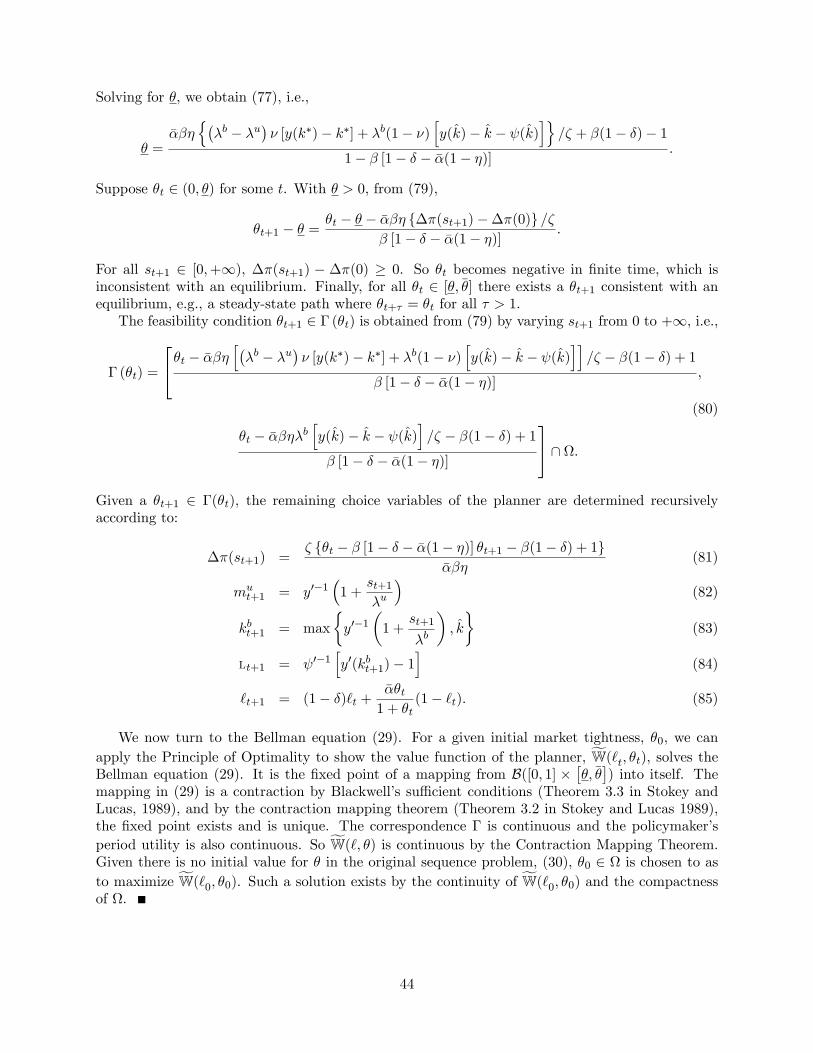
Solving for θ, we obtain (77), i.e.,

θ =αβη

(λb − λu

)ν [y(k∗)− k∗] + λb(1− ν)

[y(k)− k − ψ(k)

]/ζ + β(1− δ)− 1

1− β [1− δ − α(1− η)].

Suppose θt ∈ (0, θ) for some t. With θ > 0, from (79),

θt+1 − θ =θt − θ − αβη ∆π(st+1)−∆π(0) /ζ

β [1− δ − α(1− η)].

For all st+1 ∈ [0,+∞), ∆π(st+1) − ∆π(0) ≥ 0. So θt becomes negative in finite time, which isinconsistent with an equilibrium. Finally, for all θt ∈ [θ, θ] there exists a θt+1 consistent with anequilibrium, e.g., a steady-state path where θt+τ = θt for all τ > 1.

The feasibility condition θt+1 ∈ Γ (θt) is obtained from (79) by varying st+1 from 0 to +∞, i.e.,

Γ (θt) =

θt − αβη[(λb − λu

)ν [y(k∗)− k∗] + λb(1− ν)

[y(k)− k − ψ(k)

]]/ζ − β(1− δ) + 1

β [1− δ − α(1− η)],

(80)

θt − αβηλb[y(k)− k − ψ(k)

]/ζ − β(1− δ) + 1

β [1− δ − α(1− η)]

∩ Ω.

Given a θt+1 ∈ Γ(θt), the remaining choice variables of the planner are determined recursivelyaccording to:

∆π(st+1) =ζ θt − β [1− δ − α(1− η)] θt+1 − β(1− δ) + 1

αβη(81)

mut+1 = y′−1

(1 +

st+1

λu

)(82)

kbt+1 = max

y′−1

(1 +

st+1

λb

), k

(83)

lt+1 = ψ′−1[y′(kbt+1)− 1

](84)

`t+1 = (1− δ)`t +αθt

1 + θt(1− `t). (85)

We now turn to the Bellman equation (29). For a given initial market tightness, θ0, we canapply the Principle of Optimality to show the value function of the planner, W(`t, θt), solves theBellman equation (29). It is the fixed point of a mapping from B([0, 1] ×

[θ, θ]) into itself. The

mapping in (29) is a contraction by Blackwell’s suffi cient conditions (Theorem 3.3 in Stokey andLucas, 1989), and by the contraction mapping theorem (Theorem 3.2 in Stokey and Lucas 1989),the fixed point exists and is unique. The correspondence Γ is continuous and the policymaker’speriod utility is also continuous. So W(`, θ) is continuous by the Contraction Mapping Theorem.Given there is no initial value for θ in the original sequence problem, (30), θ0 ∈ Ω is chosen to asto maximize W(`0, θ0). Such a solution exists by the continuity of W(`0, θ0) and the compactnessof Ω.

44

Appendix A2: Endogenous theft

In our main model, the probability that the liquid assets of the entrepreneurs are embezzled, 1− ν,is exogenous. To the extent that monetary policy affects the quantity of liquid assets held byentrepreneurs, it could also affect the incentives of corporate thieves to engage in embezzlementactivities.

In order to endogenize ν, we assume that there is a unit measure of corporate thieves. Corporatethieves can be workers, managers, or accountants, or any other person who can access the liquidassets of the entrepreneur. At the start of each period, thieves exert some effort, e ∈ [0, 1], thatwill allow them to embezzle the liquid assets of the entrepreneur they will be matched with. Forinstance, they learn fraud techniques and methods to divert funds without being caught. Thecost associated with this effort is ϕ(e) with ϕ(0) = ϕ′(0) = 0, ϕ′(e) > 0, ϕ′′(e) > 0. In stage1, corporate thieves are matched at random to entrepreneurs. A thief is successful in embezzlingthe liquid assets of the entrepreneur with probability e. Thieves are risk neutral, i.e., their utilityfunction is U(c) = c.

The problem of the corporate thief within a period is:

maxe∈[0,1]

−ϕ(e) + eMt , (86)

where Mt = `tmbt + (1 − `t)mu

t is aggregate liquidity. The expected value of embezzlement corre-sponds to the second term in the maximization problem. If the thief is matched to an unbankedentrepreneur, with probability 1 − `t, then he can steal mu

t with probability e. If he is matchedwith a banked entrepreneur, with probability `t, he can steal mb

t . Assuming an interior solution,the first-order condition gives:

ϕ′(e) = Mt. (87)

The marginal cost of embezzlement on the left side is equal to the discounted aggregate liquidityon the right side. Given that the problem is strictly concave, all thieves choose the same e∗.

The probability that an entrepreneur is subject to theft is 1− ν = e∗. Hence,

ν = 1− ϕ′−1 (Mt) . (88)

From the first-order conditions (15) and (19) mbt and m

ut are independent of ν and decreasing with

s. So, if mbt < mu

t , e.g., if λb = λu = λ, then Mt is decreasing with θ and decreasing with s.

It follows from (88) that ν = 1 − e∗ is increasing with θ and s. At the Friedman rule, s = 0,ν = 1− ϕ′−1 (k∗).

We now turn to the free-entry condition of banks and the relationship it implies between θ andν = 1− e∗. Note first that

∂∆π(s)

∂ν= −λb

[y(kb)− kb − ψ(kb)

]+λb

[y(kb)− kb − ψ(l)

]− smb

−λu [y(ku)− ku]− smu

Suppose λb = λu = λ. If s is close to 0, then the last two terms on the right side are approximatelyequal. Hence, ∂∆π(s)/∂ν < 0, which implies ∂θ/∂ν < 0. As the probability of theft is reduced,the benefits from external finance are reduced as well, and hence fewer banks enter. So, from thecondition on bank entry, θ is increasing with e∗ and s.

We have two equilibrium conditions to determine jointly the pair (θ, e∗). From (87), e∗ decreaseswith θ; from bank entry, θ increases with e∗. So the pair (θ, e∗) is uniquely determined. As s

45

increases, the curve representing (87) moves to the left in the space (e∗, θ) while the free-entrycondition moves up. So, an increase in s reduces e∗.

Figure 10 illustrates the optimal policy response in the calibrated model to a 60% destructionof lending relationships when the policymaker can commitment (top three panels) and when theycannot (bottom three panels). We set ϕ(M) = κe2 and calibrate κ such that ν matches its value inTable 5.2 when the annual spread is 2%. Otherwise the parameters are kept the same as in Table5.2. The figure illustrates the optimal policy when theft is either exogenous (in solid blue) or whenit is endogenous (in dashed-red).

Figure 10: Optimal policy responses with commitment (top three panels) and without commitment(bottom three panels) with endogenous theft.

Qualitatively, the introduction of endogenous theft changes little about the optimal policyprescription. Quantitatively, we see that now the policymaker is introduced to a new tradeoff atthe onset of the shock. When the policymaker has commitment, they still lower spreads initiallyand use forward guidance about future spreads to encourage the creation of lending relationships.However by lowering spreads initially, the policy incentivizes theft so ν increases above its long-run value. The increase in theft both dampens the ability of policy to improve self-insurance andincreases the usefulness of bank lending. As a result, spreads are kept low for a shorter amount oftime and the long-run value is larger. Without commitment, the initial destruction of relationshipscauses aggregate liquidity to rise which incentivizes more theft. To counteract the increase in theft,the policymaker increases spreads by more than when ν is fixed and more gradually reduces spreadsback to a higher long-run value.

46

Appendix A3: Continuous time limit

We now derive the continuous-time limit of our model (see Choi and Rocheteau 2020 for a detailedpresentation of New Monetarist models in continuous time). We assume there is no theft and thearrival rate of investment opportunities is the same for banked and unbanked entrepreneurs. Let∆ denote the length of a period of time, where ∆ is assumed to be small. We rewrite all variablesthat have a time dimension as being proportional to ∆. It includes the matching function, theseparation rate, the rate of time preference, and the real return on liquid assets.

The law of motion of the lending relationships is

`t+∆ = (1− δ∆)`t + α(θt)∆(1− `t).

We subtract `t on both sides, divide by ∆, and take the limit as ∆ goes to zero to obtain

˙t = α(θt)(1− `t)− δ`t,

where ˙t = lim∆→0 (`t+∆ − `t) /∆.

The profits of an unbanked entrepreneur are πut ∆ where

πut = maxmt≥0

−stmt + λu max

kt≤mt

[y(kt)− kt],

where the interest spread is

st∆ =(ρ− rt) ∆

1 + rt∆.

Note that the profits conditional on an investment opportunity, y(kt) − kt, is a stock that has notime dimension. Taking the limit as ∆ goes to zero,

st = ρ− rt.

The first-order condition givesst = λu

[y′(mu

t )− 1].

The flow profits of banked entrepreneurs are unaffected,

πb(st) = maxkb,mb≥0

λb[y(kb)− kb − ψ(kb −mb)

]− stmb

.

The first-order conditions are

ψ′(kbt −mb

t

)= y′(kbt )− 1 ≤ st

λb, ”=” if mb

t > 0, ∀t.

Finally, the free-entry condition for banks is

(1 + ρ∆)θt

α(θt)∆=η[πb(st+∆)− πu (st+∆)

]∆

ζ∆− (1− η)θt+∆ + (1− δ∆)

θt+∆

α(θt+∆)∆.

Notice the cost of bank entry is a flow cost, and hence proportional to ∆. Rearranging, the equationcan be rewritten as:

1

∆

(θt

α(θt)− θt+∆

α(θt+∆)

)+ ρ

θtα(θt)

+ δθt+∆

α(θt+∆)=η[πb(st+∆)− πu (st+∆)

]ζ

− (1− η)θt+∆.

47

Taking the limit as ∆ goes to zero,

−(

1− ε(θt)α(θt)

)θ + (ρ+ δ)

θtα(θt)

=η[πb(st)− πu (st)

]ζ

− (1− η)θt,

where ε(θ) ≡ θα′(θ)/α(θ). Rearranging, we obtain:

θt =α(θt)

1− ε(θt)

(ρ+ δ)

θtα(θt)

+ (1− η)θt −η[πb(st)− πu (st)

]ζ

.

To summarize, the system of ODEs for the measure of lending relationships, credit markettightness, and the market-clearing condition for liquid assets are

˙t = α(θt)(1− `t)− δ`t (89)

θt =α(θt)

1− ε(θt)

(ρ+ δ)

θtα(θt)

+ (1− η)θt −η∆π(st)

ζ

(90)

Mt = `tmb (st) + (1− `t)mu (st) , (91)

where mu (st) and mb (st) are the implicit solutions to (15) and (19) with st ≡ ρ− rt, andMt is thesupply of liquid assets. An equilibrium is a time path, `t, θt,Mt, st, that solves (89)-(91) given`0 and monetary policy formulated either as st or Mt.

48

Appendix A4. Numerical procedures for optimal policy problems

Optimal policy with commitment

We solve for social welfare W(`, θ) and the optimal policy function θ′ = gθ(`, θ) using value functioniteration on a discrete grid.

1. Discretize the state space into N` ⊆ [0, 1] and Nθ ⊆ Ω, where the lower and upper limits ofΩ are given by solving for θt = θt+1 = θ in 25 when s is either s = 0 or s→∞.

2. Define the Bellman operator as TWn given by the right-hand side of (29).

3. Set the initial guess of W0 given by a policy consistent with a constant spread, s, defined asθ′ in

θ =αβη

ζ∆π (s) + β(1− δ)− 1 + β [1− δ − α(1− η)] θ′.

4. Update Wn+1(`, θ) = TWn(`, θ)

5. Repeat 4. until max`,θ

∥∥∥Wn+1(`, θ)− Wn(`, θ)∥∥∥ < ε. This sequence is Cauchy and converges

to the unique fixed point of T .

6. Set W (`0) = maxθ∈Ω W(`0, θ).

Optimal policy without commitment

We solve for the optimal policy functions Θ(`,mu′) and K(`) using contraction mappings on adiscrete grid.

1. Discretize the state space into N` ⊆ [0, 1] and Nm ⊆ [0, k∗], where y′∗) = 1.

2. Set the initial guess of K0(`) under a policy consistent with a constant spread, s, or s =λu [y(K(`))− 1].

3. Given Kn(`), for any n = 0, 1, 2, . . . , compute Θn(`,mu′) by iterating over the functional equa-

tion Tθ,nΘ(`,mu′) given by the right-hand side of 31. Repeat untilmax`,mu′

∥∥∥Θj+1(`,mu′)−Θj(`,mu′)∥∥∥ <

ε. This sequence is Cauchy and converges to the unique fixed point of Tθ,n, which is denotedas Θn(`,mu′).

4. Given Tθ,n from 3., update Kn+1(`) by solving the social welfare functionWn(`) using the func-tional equation TW,nW(`) given by the right-hand side of 33. Repeat untilmax` ‖Kj+1(`)−Kj(`)‖ <ε.

5. Check if ‖Kn(`)−Kn+1(`)‖ < ε. If true, stop. Else, set Kn = Kn+1 and return to 3.

Optimal policy given temporary lockdown

Solve for the optimal policy function gθ(`, θ) and social welfare function W(`, θ) under constant(λu, λb) as above. Given the length of the lockdown T > 0, solve for the optimal policy gθ,t(`, θ)and social welfare Wt(`, θ) for t = 0, . . . , T using backward induction.

1. Let WT+1 = W.

49

2. For t = 0, . . . , T , solve for Wt as

Wt(`, θ) = maxθ′∈Γt(θ)

−ζθ(1− `) + β(1− `′uν

[y(mu′)−mu′

](92)

+β`′bν[y(kb′)− kb′ − ψ(l′)

]+ (1− ν)

[y(k)− k − ψ(k)

]+ βWt+1(`′, θ′)

,

where Γt = [θt, θt] is defined iteratively by

θt = αβηζ ∆π(0) + β [1− δ − α(1− η)] θt+1 + β(1− δ)− 1

θt = αβηζ ∆π(+∞) + β [1− δ − α(1− η)] θt+1 + β(1− δ)− 1

3. Set W0(`0) = maxθ∈[θ0,θ0] W0(`0, θ).

50

Appendix A5: Ramsey problem under a timeless approach

Notice the Ramsey solution is not bound by any past promises at time t = 0, i.e., it is free to selectany equilibrium, in our context by choosing any θ0. To see how this matters, suppose the size ofthe credit shock approaches zero, i.e., the economy starts at its stationary solution. Letting thepolicymaker reset its policy is not innocuous, as illustrated in Figure ??. The policymaker reducess1 even though there is no exogenous destruction of lending relationships, which paradoxically,generates a small reduction in `.

Woodford (1999, 2003) proposed amending the Ramsey solution to discipline the initial choiceof equilibrium. We adopt a similar notion. The solution to the Bellman equation (29) givesa policy function expressed as θt+1 = Θ∗(`t, θt). Suppose the economy has an infinite history.Substituting θt = Θ∗(`t−1, θt−1) and iterating, the policy choice at t can be expressed as a functionof the entire history of lending relationships, i.e., θt+1 = Θ∞(`t, `t−1, `t−2, ...) or, equivalently,st+1 = S∞(`t, `t−1, `t−2, ...) where S∞ is a time-invariant policy function that specifies the spreadas a function of the entire history of lending relationships.

The Ramsey solution under a timeless approach sets θ0 such that θ0 = Θ∞(`−1, `−2, `−3, ...). Ifthe economy was at a steady state, then `−1 = `−2 = `−3 = `∗ and θ0 = Θ∞(`∗, `∗, `∗, ...) = θ∗.Hence, θ1 = Θ∗(`0, θ

∗) which determines s1 from the free-entry condition. In particular, if the sizeof the shock is zero, `0 = `∗, then θ1 = Θ∗(`∗, θ∗) = θ∗ and the economy remains at its stationarysolution.32 Figure 11 plots the optimal timeless policy outcomes (dashed lines) for different sizesof the shock.

Figure 11: Optimal policy: unrestricted commitment (solid) vs. timeless approach (dashed)

The Ramsey solution under a timeless approach features a hump-shaped path for the spread.By restricting θ0 to its steady-state value, the timeless approach impacts the initial spread set bythe policymaker. For small shocks, s0 is set close to its long-run value whereas for large shocks, s0

is close to zero.

32As mentioned to us by Edouard Challe, in the case of a one-off, unexpected shock, the timeless perspective doesnot fit the description of a stationary, fully state-contingent policy plan where the policymaker has planned a longtime ago how it would react to any future shock.

51

Appendix A6: Quantitative robustness

In the following, we discuss how optimal monetary policy depends on some key parameters of themodel. In the main calibration, we find ν very close to one. In the first robustness check, we lowerν to imply twice the annual probability of theft, 1 − ν, from 2.5% to 5%. Another key parameterof the model is banks’bargaining power that determines whether there is too much or too littlecreation of relationships. In our benchmark calibration, η = 0.52. Our second robustness checkreports optimal monetary policy when η ∈ 0.25, 0.75. Our third check shuts down the cost ofmonitoring loans, B = 0. In that case, the only cost of external finance is the cost of bank entry.In each case, we keep the other parameters of the model unchanged and report them in the tablebelow.

Figure 12: Robustness of optimal policy with commitment (top) and without commitment (bottom)

Figure 12 plots the optimal policy outcomes following a 60% destruction of relationships undercommitment (top panels) and without commitment (bottom panels). The main takeaway is thatthe qualitative features of our baseline example are robust. The time path of the interest spread ishump-shaped under the Ramsey solution while it is downward-sloping in the absence of commit-ment. Further, the magnitude of the spreads tend to be higher with commitment, and the recoveryof lending relationships is faster. There are two important caveats. When bank bargaining poweris high enough, optimal policy should set the spread to the lower bound. Secondly, when there isno cost to external finance, the planner maintains a spread above zero under both commitment andwithout commitment.

Specification ρ ξ δ ν α λu λb B η ζ

Baseline 0.0033 8.6 0.01 0.998 0.09 0.126 0.144 6.19 0.52 0.024ν = 0.995 0.0033 8.6 0.01 0.995 0.09 0.126 0.144 6.19 0.52 0.024η = 0.250 0.0033 8.6 0.01 0.998 0.09 0.126 0.144 6.19 0.25 0.024η = 0.750 0.0033 8.6 0.01 0.998 0.09 0.126 0.144 6.19 0.75 0.024B = 0 0.0033 8.6 0.01 0.998 0.09 0.126 0.144 0.00 0.52 0.024

52