1

Leibniz’s differential calculus applied to the catenary

Olivier Keller, agrégé in mathematics, PhD (EHESS)

Study of the catenary was a response to a challenge laid down by Jacques

Bernoulli, and which was successfully met by Leibniz as well as by Jean Bernoulli

and Huygens: to find the curve described by a piece of strung suspended from its

two ends. Stimulated by the success of this initial research, Jean Bernoulli put

forward and solved similar problems: the form taken by a horizontal blade

immobilised on one side, with a weight attached to the other; the form taken by

a piece of linen filled with liqueur; the curve of a sail.

Challenges among scholars

In the 17th century, it was customary for scholars to set each

other challenges in alternate issues of journals. Leibniz, for

example, challenged the Cartesians – as part of the

controversy surrounding the laws of collision, known as the

“querelle des forces vives” (vis viva controversy) – to find the

curve down which a body falls at constant vertical velocity

(isochrone curve). Put forward in the Nouvelle République des

Lettres of September 1687, this problem received Huygens’

solution in October of the same year, while Leibniz’s appeared

in 1689 in the journal he had created, the Acta Eruditorum.

Another famous example is that of the brachistochrone, or the

“curve of the fastest descent”, which, thanks to the new

differential calculus, proved to be not a circle, as Galileo had

believed, but a cycloid: the challenge had been set by Jean

Bernoulli in the Acta Eruditorum in June 1696, and was

resolved by Leibniz in May 1697.

It was also in this journal, in May 1690, that Jacques Bernoulli

suggested that Leibniz examine if his new calculus could solve

the problem of the catenary. Leibniz did indeed solve this

problem, though he did not publish the solution – to give other

mathematicians time to try their hand at it – until 1690.

Huygens, Jacques and Jean Bernoulli successfully solved the

problem in the imparted time.1

1. As Marc Parmentier indicates in his annotations accompanying Leibniz’s text (Éditions Vrin): “The historical prestige of the question and the competition solemnly installed by Leibniz had put the catenary in everyone’s minds and in the years to come paved its way to the career of the new cycloid. However, the particularity of the

2

Figure 1: Brachistochrone curve. The arc of the cycloid AB (in red)

is the curve through which a weight leaving from A will arrive at B in

the shortest amount of time.

It should be noted that some of the curves studied by Leibniz were already

known, and that many of their properties had already been established through

purely geometric means or pre-differential methods. The cycloid, for example,

was one such case, but differential calculus could pride itself on having

considerably simplified the proofs of the properties already established. In

contrast, the catenary was a curve discovered thanks to the new calculus,

which could therefore boast of having genuinely advanced the art of inventing, of

which Leibniz so fond. Moreover, the author implies that he was the first to have

noticed and used the link between this curve and logarithms, a link that makes it

possible to “construct” the latter simply with a suspended piece of string.

Indeed, I observed that the fecundity of this curve is equalled only by the

ease by which it is realised, which places it ahead of all the Transcendents

[transcendental curves]. In fact, we can obtain and trace it with little

difficulty, through a physical type of construction, by hanging a piece of

string or better still a catenary (of invariable length). And once, thanks to

this, we have its outline, we can bring to light … all the Logarithms we

may wish …

We will untangle Leibniz’s difficult text by first giving the differential

equation of the catenary, which, though it forms the basis of the text, is absent

from it. From this, we will deduce point by point the construction of the catenary,

and, inversely, the construction of logarithms from a “suspended piece of string”.

Finally, we will deduce some of the properties of the catenary, stated by the

author without demonstration.

catenary, which no doubt contributed to its prestige, is that it is not a mechanical curve in Descartes’ sense, but a static curve. As such, it outclasses the cycloid in the scale of the transcendent curves to the extent that it cannot be constructed through a composition of movements.”

3

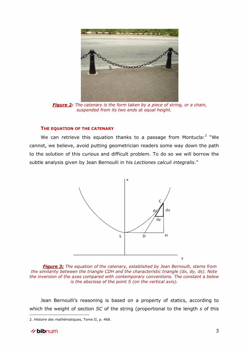
Figure 2: The catenary is the form taken by a piece of string, or a chain,

suspended from its two ends at equal height.

THE EQUATION OF THE CATENARY

We can retrieve this equation thanks to a passage from Montucla:2 “We

cannot, we believe, avoid putting geometrician readers some way down the path

to the solution of this curious and difficult problem. To do so we will borrow the

subtle analysis given by Jean Bernoulli in his Lectiones calculi integralis.”

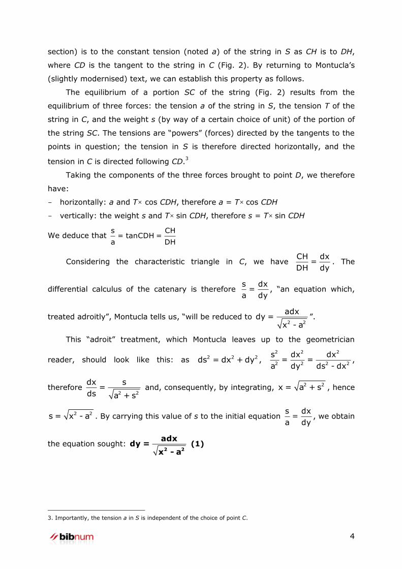
Figure 3: The equation of the catenary, established by Jean Bernoulli, stems from

the similarity between the triangle CDH and the characteristic triangle (dx, dy, ds). Note

the inversion of the axes compared with contemporary conventions. The constant a below

is the abscissa of the point S (on the vertical axis).

Jean Bernoulli’s reasoning is based on a property of statics, according to

which the weight of section SC of the string (proportional to the length s of this

2. Histoire des mathématiques, Tome II, p. 468.

4

section) is to the constant tension (noted a) of the string in S as CH is to DH,

where CD is the tangent to the string in C (Fig. 2). By returning to Montucla’s

(slightly modernised) text, we can establish this property as follows.

The equilibrium of a portion SC of the string (Fig. 2) results from the

equilibrium of three forces: the tension a of the string in S, the tension T of the

string in C, and the weight s (by way of a certain choice of unit) of the portion of

the string SC. The tensions are “powers” (forces) directed by the tangents to the

points in question; the tension in S is therefore directed horizontally, and the

tension in C is directed following CD.3

Taking the components of the three forces brought to point D, we therefore

have:

­ horizontally: a and T× cos CDH, therefore a = T× cos CDH

­ vertically: the weight s and T× sin CDH, therefore s = T× sin CDH

We deduce that s CH

= tanCDH =a DH

Considering the characteristic triangle in C, we have CH dx

=DH dy

. The

differential calculus of the catenary is therefore s dx

=a dy

, “an equation which,

treated adroitly”, Montucla tells us, “will be reduced to 2 2

adxdy =

x - a”.

This “adroit” treatment, which Montucla leaves up to the geometrician

reader, should look like this: as 2 2 2ds = dx + dy , 2 2 2

2 2 2 2

s dx dx= =

a dy ds - dx,

therefore 2 2

dx s=

ds a + s and, consequently, by integrating,

2 2x = a + s , hence

2 2s = x - a . By carrying this value of s to the initial equation s dx

=a dy

, we obtain

the equation sought: 2 2

adxdy =

x - a (1)

3. Importantly, the tension a in S is independent of the choice of point C.

5

Note that we obtain the equation4 of only part of the curve, the increasing

part, because the coordinates are pairs of positive numbers. The difficulties that

such a restriction might raise, at a time when negative numbers were not yet

recognised as legitimate, can possibly be compensated here by symmetrical

considerations: we have the same curve “on the other side”.

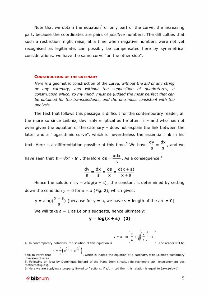
CONSTRUCTION OF THE CATENARY

Here is a geometric construction of the curve, without the aid of any string

or any catenary, and without the supposition of quadratures, a

construction which, to my mind, must be judged the most perfect that can

be obtained for the transcendents, and the one most consistent with the

analysis.

The text that follows this passage is difficult for the contemporary reader, all

the more so since Leibniz, devilishly elliptical as he often is – and who has not

even given the equation of the catenary – does not explain the link between the

latter and a “logarithmic curve”, which is nevertheless the essential link in his

text. Here is a differentiation possible at this time.5 We have

dy dx=

a s, and we

have seen that 2 2s = x - a , therefore

xdxds =

s. As a consequence:

6

dy dx ds d(x + s)= = =

a s x x + s

Hence the solution isy = alog(x + s) ; the constant is determined by setting

down the condition y = 0 for x = a (Fig. 2), which gives:

x + sy = alog( )

a (because for y = o, we have s = length of the arc = 0)

We will take a = 1 as Leibniz suggests, hence ultimately:

y = log(x + s) (2)

4. In contemporary notations, the solution of this equation is

2

x xy = a ln + - 1

a a

. The reader will be

able to verify that

y y-

a aa

x = e + e

2 , which is indeed the equation of a catenary, with Leibniz’s customary inversion of axes. 5. Following an idea by Dominique Bénard of the Mans Irem (Institut de recherche sur l’enseignement des mathématiques). 6. Here we are applying a property linked to fractions, if a/b = c/d then this relation is equal to (a+c)/(b+d).

6

We observed above that equation (1) concerns only half of the curve. The

other half, which is symmetrical to the first in relation to the vertical axis, will

have the following equation:

1y = - log(x + s) = log = log(x - s)

x + s

(3)

since 2 2 2(x - s)(x + s) = x - s = a =1 .

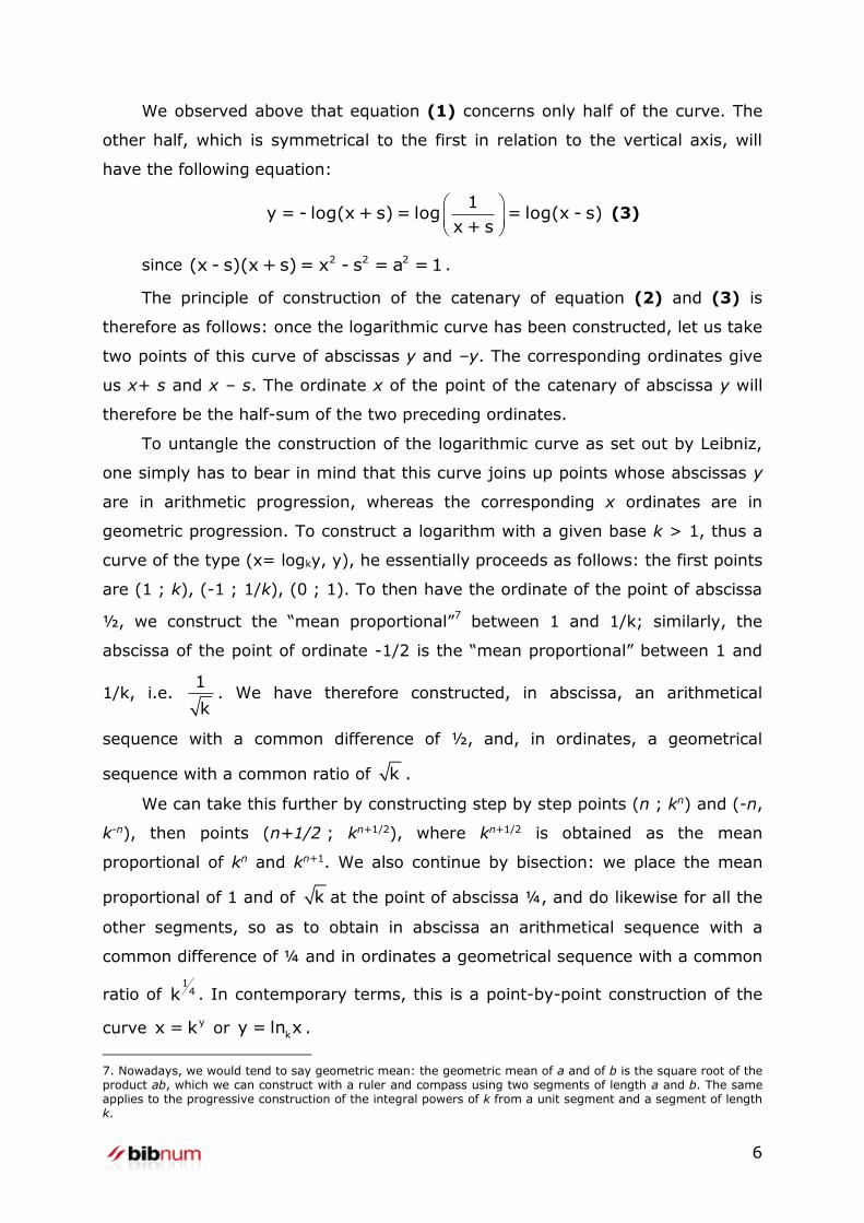
The principle of construction of the catenary of equation (2) and (3) is

therefore as follows: once the logarithmic curve has been constructed, let us take

two points of this curve of abscissas y and –y. The corresponding ordinates give

us x+ s and x – s. The ordinate x of the point of the catenary of abscissa y will

therefore be the half-sum of the two preceding ordinates.

To untangle the construction of the logarithmic curve as set out by Leibniz,

one simply has to bear in mind that this curve joins up points whose abscissas y

are in arithmetic progression, whereas the corresponding x ordinates are in

geometric progression. To construct a logarithm with a given base k > 1, thus a

curve of the type (x= logky, y), he essentially proceeds as follows: the first points

are (1 ; k), (-1 ; 1/k), (0 ; 1). To then have the ordinate of the point of abscissa

½, we construct the “mean proportional”7 between 1 and 1/k; similarly, the

abscissa of the point of ordinate -1/2 is the “mean proportional” between 1 and

1/k, i.e. 1

k. We have therefore constructed, in abscissa, an arithmetical

sequence with a common difference of ½, and, in ordinates, a geometrical

sequence with a common ratio of k .

We can take this further by constructing step by step points (n ; kn) and (-n,

k-n), then points (n+1/2 ; kn+1/2), where kn+1/2 is obtained as the mean

proportional of kn and kn+1. We also continue by bisection: we place the mean

proportional of 1 and of k at the point of abscissa ¼, and do likewise for all the

other segments, so as to obtain in abscissa an arithmetical sequence with a

common difference of ¼ and in ordinates a geometrical sequence with a common

ratio of 1

4k . In contemporary terms, this is a point-by-point construction of the

curve yx = k or k

y = ln x .

7. Nowadays, we would tend to say geometric mean: the geometric mean of a and of b is the square root of the product ab, which we can construct with a ruler and compass using two segments of length a and b. The same applies to the progressive construction of the integral powers of k from a unit segment and a segment of length k.

7

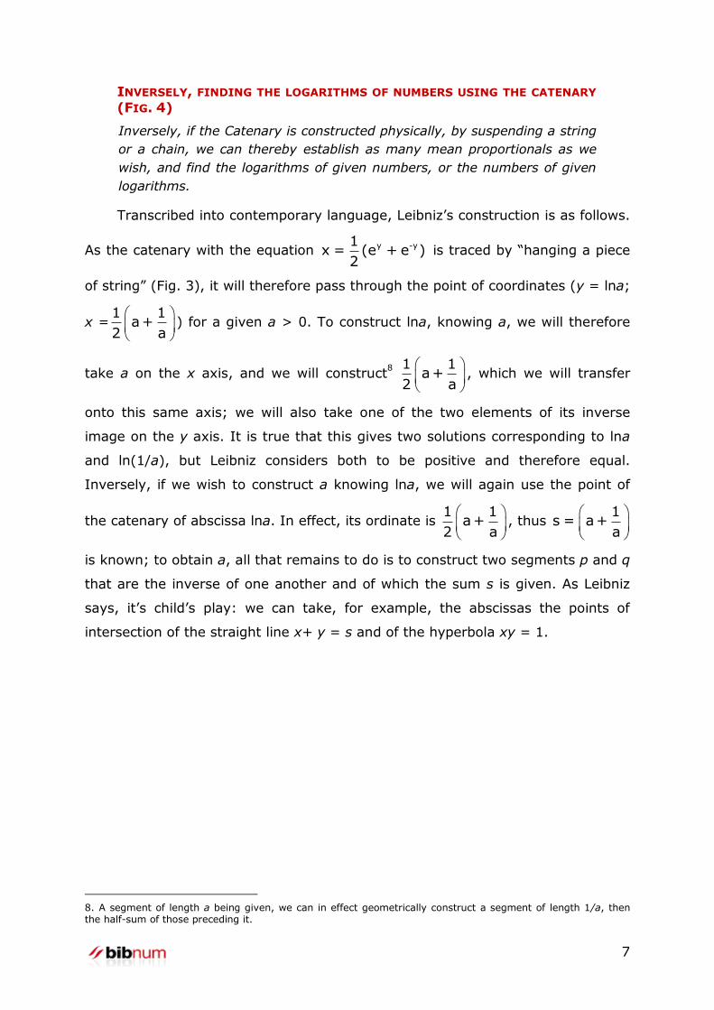
INVERSELY, FINDING THE LOGARITHMS OF NUMBERS USING THE CATENARY

(FIG. 4)

Inversely, if the Catenary is constructed physically, by suspending a string

or a chain, we can thereby establish as many mean proportionals as we

wish, and find the logarithms of given numbers, or the numbers of given

logarithms.

Transcribed into contemporary language, Leibniz’s construction is as follows.

As the catenary with the equation y -y1x = (e + e )

2 is traced by “hanging a piece

of string” (Fig. 3), it will therefore pass through the point of coordinates (y = lna;

x =1 1

a+2 a

) for a given a > 0. To construct lna, knowing a, we will therefore

take a on the x axis, and we will construct8 1 1

a+2 a

, which we will transfer

onto this same axis; we will also take one of the two elements of its inverse

image on the y axis. It is true that this gives two solutions corresponding to lna

and ln(1/a), but Leibniz considers both to be positive and therefore equal.

Inversely, if we wish to construct a knowing lna, we will again use the point of

the catenary of abscissa lna. In effect, its ordinate is 1 1

a+2 a

, thus 1

s = a+a

is known; to obtain a, all that remains to do is to construct two segments p and q

that are the inverse of one another and of which the sum s is given. As Leibniz

says, it’s child’s play: we can take, for example, the abscissas the points of

intersection of the straight line x+ y = s and of the hyperbola xy = 1.

8. A segment of length a being given, we can in effect geometrically construct a segment of length 1/a, then the half-sum of those preceding it.

8

Figure 4: Construction of lna from the outline of the catenary (here, for example, we

have taken a=2).

The author then states a whole series of the catenary’s properties without

any demonstration, indeed without even giving an equation for the curve. We are

now going to recover these properties using the instruments of the time, in the

manner of the author of a late 17th-century textbook.

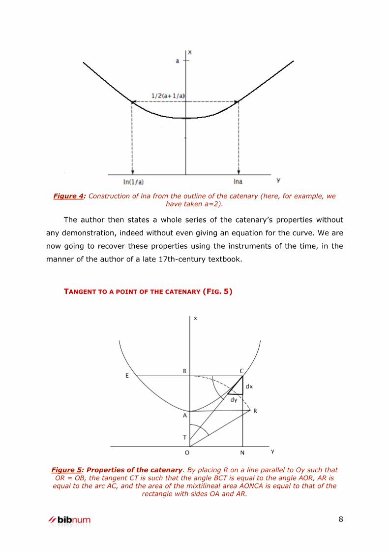
TANGENT TO A POINT OF THE CATENARY (FIG. 5)

Figure 5: Properties of the catenary. By placing R on a line parallel to Oy such that

OR = OB, the tangent CT is such that the angle BCT is equal to the angle AOR, AR is

equal to the arc AC, and the area of the mixtilineal area AONCA is equal to that of the

rectangle with sides OA and AR.

9

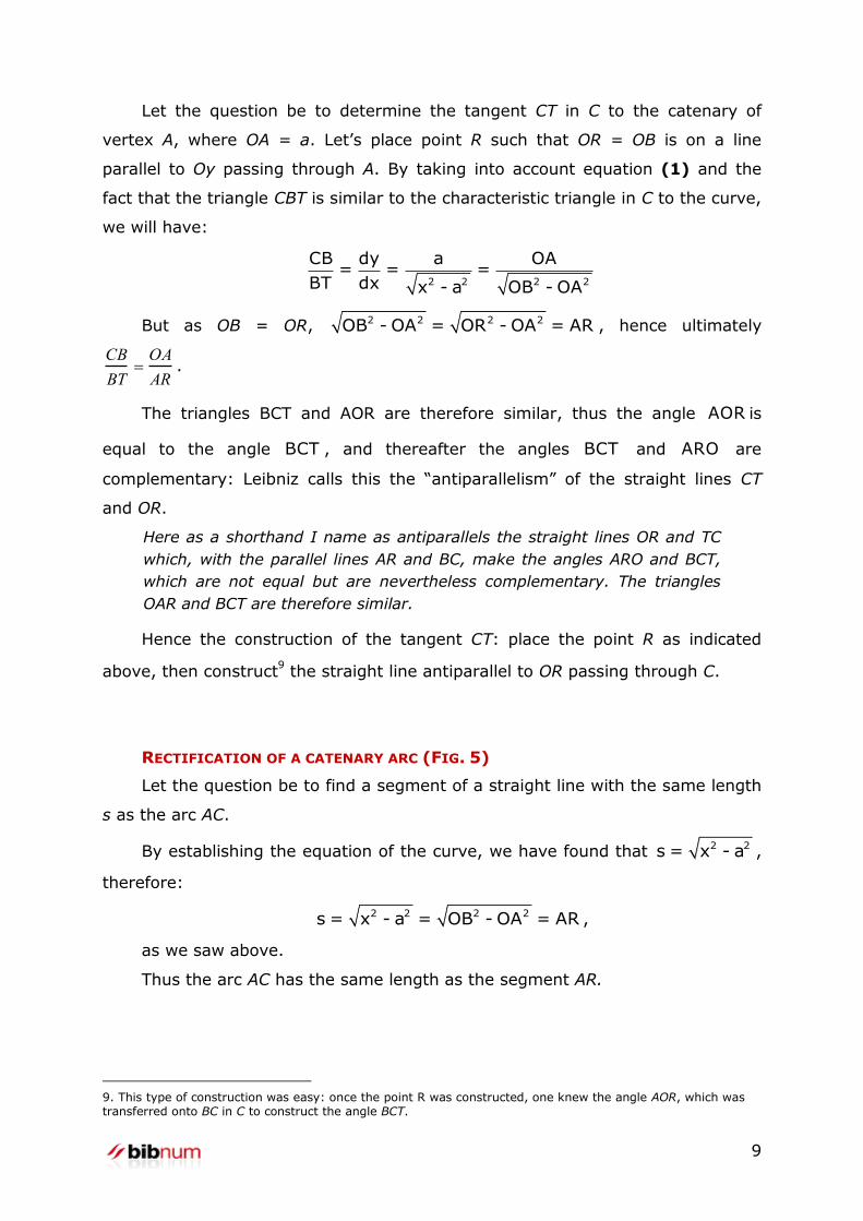
Let the question be to determine the tangent CT in C to the catenary of

vertex A, where OA = a. Let’s place point R such that OR = OB is on a line

parallel to Oy passing through A. By taking into account equation (1) and the

fact that the triangle CBT is similar to the characteristic triangle in C to the curve,

we will have:

2 2 2 2

CB dy a OA= = =

BT dx x - a OB - OA

But as OB = OR, 2 2 2 2OB - OA = OR - OA = AR , hence ultimately

CB

BTOA

AR.

The triangles BCT and AOR are therefore similar, thus the angle AOR is

equal to the angle BCT , and thereafter the angles BCT and ARO are

complementary: Leibniz calls this the “antiparallelism” of the straight lines CT

and OR.

Here as a shorthand I name as antiparallels the straight lines OR and TC

which, with the parallel lines AR and BC, make the angles ARO and BCT,

which are not equal but are nevertheless complementary. The triangles

OAR and BCT are therefore similar.

Hence the construction of the tangent CT: place the point R as indicated

above, then construct9 the straight line antiparallel to OR passing through C.

RECTIFICATION OF A CATENARY ARC (FIG. 5)

Let the question be to find a segment of a straight line with the same length

s as the arc AC.

By establishing the equation of the curve, we have found that 2 2s = x - a ,

therefore:

2 2 2 2s = x - a = OB - OA = AR ,

as we saw above.

Thus the arc AC has the same length as the segment AR.

9. This type of construction was easy: once the point R was constructed, one knew the angle AOR, which was transferred onto BC in C to construct the angle BCT.

10

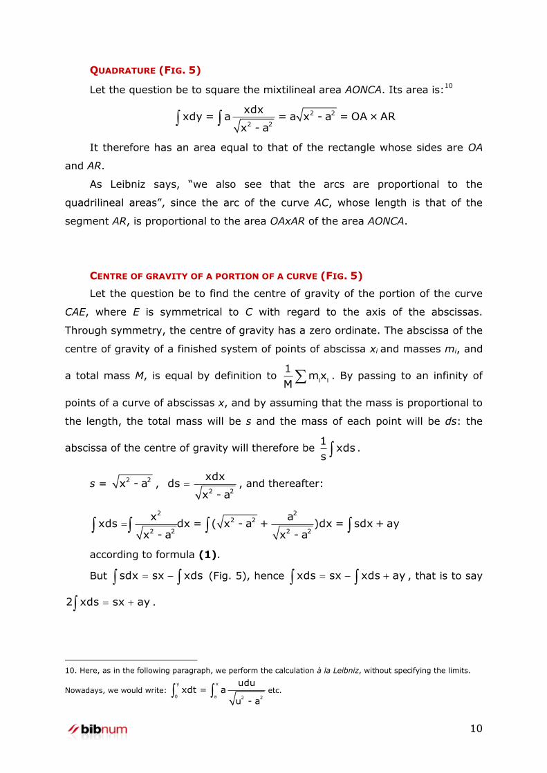
QUADRATURE (FIG. 5)

Let the question be to square the mixtilineal area AONCA. Its area is:10

2 2

2 2

xdxxdy = a = a x - a = OA × AR

x - a

It therefore has an area equal to that of the rectangle whose sides are OA

and AR.

As Leibniz says, “we also see that the arcs are proportional to the

quadrilineal areas”, since the arc of the curve AC, whose length is that of the

segment AR, is proportional to the area OAxAR of the area AONCA.

CENTRE OF GRAVITY OF A PORTION OF A CURVE (FIG. 5)

Let the question be to find the centre of gravity of the portion of the curve

CAE, where E is symmetrical to C with regard to the axis of the abscissas.

Through symmetry, the centre of gravity has a zero ordinate. The abscissa of the

centre of gravity of a finished system of points of abscissa xi and masses mi, and

a total mass M, is equal by definition to i i

1mx

M . By passing to an infinity of

points of a curve of abscissas x, and by assuming that the mass is proportional to

the length, the total mass will be s and the mass of each point will be ds: the

abscissa of the centre of gravity will therefore be 1

xdss

.

s = 2 2x - a ,

2 2

xdxds

x - a , and thereafter:

2 22 2

2 2 2 2

x axds dx = ( x - a + )dx = sdx + ay

x - a x - a

according to formula (1).

But sdx sx xds (Fig. 5), hence xds sx xds ay , that is to say

2 xds sx ay .

10. Here, as in the following paragraph, we perform the calculation à la Leibniz, without specifying the limits.

Nowadays, we would write: y x

0 a 2 2

uduxdt = a

u - a etc.

11

The abscissa of the centre of gravity is therefore:

1 1 ay 1 OA ×BCxds = (x + ) = (OB + )

s 2 s 2 AR . This last formula corresponds to the

construction indicated by Leibniz, since the “proportional fourth”11

z of AR, BC

and OA is defined by AR OA

=BC z

, hence OA ×BC

z =AR

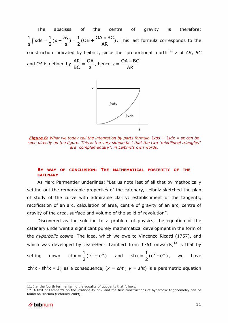
Figure 6: What we today call the integration by parts formula ∫xds + ∫sdx = sx can be

seen directly on the figure. This is the very simple fact that the two “mixtilineal triangles”

are “complementary”, in Leibniz’s own words.

BY WAY OF CONCLUSION: THE MATHEMATICAL POSTERITY OF THE

CATENARY

As Marc Parmentier underlines: “Let us note last of all that by methodically

setting out the remarkable properties of the catenary, Leibniz sketched the plan

of study of the curve with admirable clarity: establishment of the tangents,

rectification of an arc, calculation of area, centre of gravity of an arc, centre of

gravity of the area, surface and volume of the solid of revolution”.

Discovered as the solution to a problem of physics, the equation of the

catenary underwent a significant purely mathematical development in the form of

the hyperbolic cosine. The idea, which we owe to Vincenzo Ricatti (1757), and

which was developed by Jean-Henri Lambert from 1761 onwards,12

is that by

setting down x -x1chx = (e + e )

2 and x -x1

shx = (e - e )2

, we have

2 2ch x - sh x = 1; as a consequence, (x = cht ; y = sht) is a parametric equation

11. I.e. the fourth term entering the equality of quotients that follows. 12. A text of Lambert’s on the irrationality of and the first constructions of hyperbolic trigonometry can be

found on BibNum (February 2009).

12

of the hyperbola 2 2x - y =1 . With regard to the hyperbola, the hyperbolic cosine

ch and the hyperbolic sine sh therefore play a role analogous to that which the

ordinary cosine and sine have with regard to the circle, since (x = cost ; y = sint)

is a parametric equation of the unit circle.13

The catenary (with the equation y = ch x), revealed through the analysis of

its physical properties, would thus be at the origin of two important mathematical

developments: hyperbolic trigonometry and differential calculus.

(March 2009)

(This text was revised and adapted by the author on the basis of the IREM book he

coordinated, Textes fondateurs du calcul infinitésimal, 2006, with the kind permission of

Éditions Ellipses)

(Translated by Helen Tomlinson, published April 2017)

13. Especially since, as Euler had established in 1740, we have ix -ix1

cosx = (e + e )2

and

ix -ix1sinx = (e - e )

2i.