LEHIGH U I ER IT
135
A PRESTRESSED CONCRETE BOX-BEAM BRIDGE by STRUCTURAL BEHAVIOR OF ER IT I Yan-Liang Chen M. S. THESIS DEPARTMENT OF CIVIL ENGINEERING FRITZ ENGINEERING "LABORATORY REPORT NO. 315.10T LEHIGH U
Transcript of LEHIGH U I ER IT
A PRESTRESSED CONCRETE BOX-BEAM BRIDGE
by
STRUCTURAL BEHAVIOR OF
ER ITI
Yan-Liang Chen
M. S. THESISDEPARTMENT OF CIVIL ENGINEERING
FRITZ ENGINEERING "LABORATORY REPORT NO. 315.10T
LEHIGH U
STRUCTURAL BEHAVIOR OF
A PREsTRESSED CONCRETE BOX-BEAM BRIDGE
HAZLETON BRIDGE
by
Yan-Liang Chen
A THESIS
Presented to the Graduate Committee
of Lehigh University
in Candidacy for the Pegree of
Master of Science
in Civil Engineeri~g
Lehigh University
Bethlehem, Pennsylvania
August, 1970
CERTIFICATE OF APPROVAL
This thesis is accepted and approved in partial
fulfillment of the requirements of the degree of Master
of Science.
Dr·. David A. VanHornProfessor in Charge and ChairmanDe~artment of Civil Engineering
ii
TABLE OF CONTENTS
ABSTRACT
1. INTRODUCTION
1.1 Background
1.2 Objectives
1.3 Previous Studies
2. DESCRIPTION OF TEST PROGRAM
2.1 Test Bridge
2·. 2 Instrwnentation
2.2.1 ,Gaged Sections and Gage Locations
2.2.2 Position and Timing Indicators
2 • 3 Test 'Loading .
2.3.1 Test Vehicle
2.3.2 Test'Lanes
2.3.3 Test Runs
3~ DATA REDUCTION AND EVALUATION
3.1 Oscillograph Reading
3.2 Evaluation of Oscillograph Data
1
1
3
3
6
6
7
7
8
8
8
9
9
11
11·
11
3.2.1
3.2.2
3.2.3
3.2.4
Strains and Neutral Axes
Moment Coefficients and DistributionCoefficients
Distribution Influence Lines andDistribution Factors
Deflections and Deflection InfluenceLines
iii
11
12
13
13
3.2.5 Dynamic Load Factors andImpact Factors
3.3 Frequency, Logarithmic Decrement
4. COMPUTATION OF MOMENT COEFFICIENTS
~.l The First Method
14
17
19
19
..... 1.1
4.1.2
4.1.3
4.1.'-t
If..l.5
4.1.6
11-.1.7
4.1.8
Linear Strain Distribution
Consideration of Parapet
Use of Symmetry and Superposition
The Modular Ratio
Linear Variation of Slab Strains
Support Restraints
Effective Slab Widths
Computation Procedure
19
20
20
20
21
21
.21
22
4.2 The Second Method
-..... 2.1 -Basic Assumptions
4.2.2 Support Restraints
4.2.3 Slab Widths
4.2.4 The Analytical Procedure of theSecond Method
5. PRESENTATION OF TEST RESULTS
. 5.1 General
5.2 ·Moment Coefficients, Elastic Modulus
5.3 Distribution Coefficients
5.4 Distribution· Influence Lines andDistribution Factors
5.5 Deflections and Deflection Influence' Lines
5.6 Dynamic Load Factors and Impact Factors
iv
22
22
23
23
24
27
27
27
28
28
29
30
5.7 Neutral Axes
5 . 8 Effective S]~ab Widths '.
5.9 Frequencies
5.10 Logarithmic Decrement
6. DISCUSSION OF RESULTS
6.1 Static Live Load Effect
31
31
32
32
34
34
6.1.1
6.1.2
6.1.3
Distribution Factors
Beam Deflection
Neutral Axes
34
36
37
6.2" Moving Load Effect 37
6.2.1
6.2.2
6.2.3
6.2.4-
,6.2.5
6.2.6
Moment Coefficients
Distribution Coefficients
Dynamic Load Factors
Frequencies
Damping Effect
Neutral Axes
·37
38
38
'39
42
42
6.3 Impact Loading Effect 43
6.3.1
6.3.2
6.3.3
Distribution Coefficients
Moment Coefficients and Impact Factors
Neutral Axes
43
43
44
6.4 End'Restraint Effect 44
6.4.1
6.4.2
6.4.3
6.4.4
6.4.5
Distribution Coefficients
Moment Coefficients
Modulus of Elasticity
Dynamic Load Factors and Impact Factors
Effective Slab Widths
v
44
45
4S
46
46
Page
7 . SUMMARY AND CONCLUSIONS 48
7.1 Summary 48
7.2 Conclusions 49
8. ACKNOWLEDGMENTS 52
9. TABLES 54
10. FIGURES 83
11. REFERENCES 123
12. VITA 126
vi
· , ABSTRACT
This report describes the field testing of an in-service
beam-slab highway bridge· constructed with prestressed concrete
spread-box beams. The principal objectives of this study were to
experimentally investigate the dynamic effect of moving vehicle
loading and vehicle impact loading, and to provide additional in
formation on lateral load distribution of the bridge under static
vehicle loading. The testing program consisted of the continuous
reading of beam surface strains and beam deflections at tIle maxi
mum moment section of a simply supported span, as a test vehicle
was driven over the test span at speeds ranging from 2.5 mph to
60 mph, including 10 mph, 2-inch drop, impact runs.
It- was found that the experimentally determined distri
bution factors for interior beams were substantially less than the
values used in design of the superstructure, whereas the experi
mental vallles for exterior be-arns were greater than design values.
It would be desirable to include the effect of curb and parapet in
future design procedures for distribution factors. The lateral
load distribution for speed runs and impact runs was found to be
more nearly uniform than that for crawl runs.
It was found that the dynamic load factors were not
linearly related to the speed of the vehicle. It was also found
that the maximlll1l amplification of bridge vibrati'ons was reached
when the observed load frequency of forced vibrations was
'approximately equal to the "natural unloaded frequency of bridge.
The magnitude of amplification of bridge vibration under the
10 mph, 2-inch drop, impact loading was twice as large as that
under 2.5 mph crawl run loading. The experimental unloaded
natural frequency of the bridge was found to be in close agree
ment with a theoretical value. In addition, both methods used in
this study" to obtain experimentally determined beam moments could
be utilized to analyze the structural response of the prestressed
concrete box-beam bridge.
I. INTRODUCTION
1.1 Background
Since the use of prestressed concrete in the. Walnut Lane
Bridge in Philadelphia, many improvements and new concepts have
been introduced in the design of prestressed concrete bridges in
the United States. One of the developments which has been used
extensively in Pennsylvania, is the design and construction of
spread box-beam bridges. In· these bridges, the box-beams are
incorporated into a beam-slab superstructure with the beams
spread apart, as in typical I~beam bridges.
For the design of spread box-beam superstructures, the
Pennsylvania Department of Highways has utilized provisions for
distribution of design loads which parallel parts of Section 1.3.1
of the AASHO Specifications for Highway Bridges. 1 According to
the PDH Standards,2 the interior beams should be designed using a
live-load distribution factor of 8/5.5, where S is the average
beam spacing in feet. The distributio11 of live' .load ':to ':theexter
ior beams is determined by applying to the beam the reaction of a
wheel load obtained by assuming that the slab acts as a simple
span between beams.
Since it was felt that this procedure for load distri
bution could be suitably modified, and since the~design criteria
developed for adjacen~ box-beams was not applicable, a research
program was initiated at Lehigh University, basically to:
-1-
(1) develop the information needed to evaluate the load distribu-
tiOD in bridges of current design, (2) develop a mathematical
analysis which will accurately represent the structural response
to vehicle loading, and (3) develop a new specification provision.
The over-all investi.gation consisted of the field testing of five
in-service bridges in Pennsylvania. In the summer of 1964, the
Drehersville Bridge was tested to serve as a pilot study.
Bridges at Broo'kville, Berwick, and White Haven were tested in the
summer of 1965 basically to study the effects of skew and beam
width. In 1966, the Philadelphia Bridge was tested primarily
to study the effect of the midspan diaphragms on load distribu-
tiona The four-year study was completed in 1968, and eight
3 4 5 6 7 8 9 10reports ", , , ., " have been completed and distributed.
Based on the test results and conclusions included in
the initial four-year study, it was decided that a sixth spread
box-bea.m bridge should be instrumented and subjected to design
vehicle loading which would include speeds ranging from 2 mph to
60 mph. Previous studies by Linger and Hulsbos 1.1
., had indicated
that at least one, and possibly two, critical speeds for the
design vehicle may occur in this range, where critical speed is
defined as the speed at which maximum amplification of crawl-run
response is achieved. Therefore, it was felt that additional
information was needed to more clearly evaluate the superstruc-
ture response to moving vehicles, and further, that studies of
controlled impact loading and of slab behavior would be
-2-
desirable. It \-vas felt tllat this additional information would
provide valuable information in supplementing the previous study
of distribution of vehicle loading in spread box-beam bridges.
1.2 Objectives
In the summer of 1968, the Hazleton Bridge was field
tested to develop the desired information. The major objectives
of the Hazleton Bridge study were: (1) To establish critical
speeds at which maximum amplification of crawl-run response· is
achieved, and to determine the magnitude of the maximum amplifi-
cation, (2) to establi.sh the amplification of crawl-run response
under controlled impact loading, (3) to develop information on
stresses on the surface of the slab in both lateral and longitudi~
·nal directions, (4) to develop information on stress in slab
reinforcement, and (5) to provide additional information on later-
al distribution of design vehicle loading.
This report describes part of the results from the
Hazleton Bridge field test, namely those associated with objec-
tives (1), (2), and (5). The results related to objectives (3)
and _(4) wiJ_l be described in another report.
1.3 Previous Studies
The previous studies which covered the field work and
the theoretical analysis of the bridge behavior under static
3 5vehicle loading were described in Reports Nos. 315.1, 315.4,
6 7 8 10315.5, 315.6, 315.7, and 315.9. However, some other studies
-3-
which have contributed to the dynamic behavior of bridges are
significant.
Dynamic behavior has been studied in many countries and
institutions, first in railroad brid,ges, then in high\vay bridges.
The principal concern in all studies, especially the early ones,
was the formulation of the problem. In practically all cases, the
results led to the conclusion that excessive vertical displace
ments will be caused if the forcing frequency approaches the
natural frequency of the bridge. This forcing frequency was
expressed either as a function of a sinusoidal, time dependent
forcing function, or as a function of a series of concentrated
loads representing moving vehicle wheel loads.
In the United States, two significant test programs were
conducted, one at the Massachusetts Institute of Technology, and
another at Iowa State University. In 1959, simple-span beam
bridges and stringer bridges, loaded with single vehicles, were
studied at MIT by Biggs, Suer, and LOUW.12
The theoretical
analysis which was developed was accompanied by a model study and
field study. These studies indicated that the initial amplitude
of vehicle oscillation is the most important factor influencing
the magnitude of bridge vibration, and that large vibrations
generally occur when the natural frequency of the vehiCle is
close to the natural frequency of the unloaded bridge. An
equation for the experimental natural frequency of a bridge was
vresented as the product of an experimentally determined constant,
1.2, and the theoretical. expression for first-mode natural fre-
quency of a simple-span, uniform beam.13
In 1963, Louw expanded
the earlier work of Biggs, Suer, and Louw to cover the case of a
two-span continuous bridge.
In 1960 at Iowa State University, Linger and Hulsbos11
reported a theoretical analysis and field test study which
included coverage of both simple and continuous span bridges.
It was reported that the theoretical unloaded natural frequencies
of the bridges, neglecting damping, agreed very well with the
experimentally determined unloaded frequencies. Theoretical
equations were also developed for the loaded natural frequency
of various bridges, and" for dynamic load factors (impact factors).
In addition, a good qualitative correlation was found between the
magnitude of impact 'and the nearness of the frequency of axle
repetition to the loaded na~ural frequency of t~e structure.
Additional studies, of dynamic behavior are listed in
the paper by Varney and Galambos.l 4
-5-
2. DESCRIPTION OF TEST PROGRAM
2.1 Test Bridge
The Hazleton Bridge, located on L.R. 1009, Sec. 93 over
L.R. 170 in Luzerne County~ Pennsylvania, was selected for the
field test. The middle span of the three-span bridge, as illus
trated in Fig. 1, was chosen as the test span. The test span is
·simply supported with a length of 69 feet 7 inches, center-to
center of bearings. The skew is 88°-25 1• The cross-section of
the bridge is shown in Fig. 2. The superstructure is composed of
five identical prestressed concrete hollow box-beams, which are
48 inches wide and 42 inches deep, and equally spaced at 9 feet
6 inches, center-to-center. Midspan and end diaphragms, along
with the reinforced concrete slab, were cast-in-place. The slab,
which had a specified minimum thickness of 7-1/2 inches, provides
a roadway width of 40 feet. However, measurements of slab thick
ness taken near midspan ranged from 7.9 to 9.0 inches~ with an
average of 8.2 inches. The eurb and parapet sections were east
in-place after the slab concrete had reached the specified
strength in the construction sequence. The joint between the slab
and the curb section is strengthened by vertical reinforcement
which extends from the slab up into the curb section.
The design highway live loading was HS 20-44, and the
AASH0 1 impact formula was used ..All interior beams were designed
utilizing a distribution factor of 8/5.5 = 1~727, while the factor
-6-
of 1.158 was used for exterior beams. The specified minimum 28-day
cylinder strength of the beam concrete was 5500 psi. Further de-
tails of the design and construction of the bridge are given in
the PDH Standards for Prestressed Concrete Bridges.2
2.2 Instrumentation
2.2.1" Gaged Sections and Gage Locations
Two cross-sections, designated as Sect~ons M and Q, were
selected for gaging. The locations of these. cross-sections are
shown in Fig. 1. Section M was located 3.55 feet east of midspan,
and is the section where the theoretical maximum live load moment
would occur, with the live load vehicle moving eastward. Section
Q was located 16.75 feet east of midspan, near the quarter-point
of' the span.
As shown in Fig. 3, four strain gages were applied on .
each side of each of the three gaged beams.. One gage was located
at the bottom face, and the others were installed 6-1/4 inches,
15 inches, and 38-1/4 inches, respectively, from the bottom face
of the beam. Since the cross-section was symmetrical, only
Beams A, B, and C were gaged. All of the beam gages were located
at Section M. Transverse gages on the surface of the concrete,
and gages on the transverse slab reinforcement, were applied at
both Sections M and Q, as shown in Fig.~. This report will not
include the results obtained from the transverse slab gages and
the slab reinforcement gages.
-7-
The deflection gages were applied at Section M on the
middle of the bottom face of each of the gaged beams.
2.2.2 Position and Timing Indicators
Three air hoses were used as position indicators. They
were placed at Section M, and 40 feet each way from Section M.
The distances were measured along the roadway center-line, and
the hoses were placed normal to that center-line. Vehicular
wheel contacts ,with these three hoses prqduced offsets on the
oscillograph traces. The offsets were used later to correlate
the location of the load vehicle with strain values in the data
reduction. Two additional hoses, 180 feet apart, were used as
timer hoses to monitor the speed of the test vehicle. A timer
was actuated as the front axle of the approaching vehicle passed
over the first of the timer hoses, and was shut off as the tront
axle passed over the second 'timer hose. The lateral position
indicator consisted of a line of wooden slats mounted to pivot
on a horizontal rod. Before each test run, all of the slats were
positioned vertically. During the pass of the load vehicle, a
vertical rod mounted on the center-line at the front of the
vehicle would displace one or two slats, thereby indicating the
lateral vehicle location as the vehicle passed over the bridge.
2.3 Test Loading
2.3.1 Test Vehicle
The test vehicle used in this study was a three-axle
-8-
diesel tractor semi-trailer combination which, when properly loaded
with aggregate material, closely simulated an HS 20-44 design
vehicle. The axle loads and dimensions of the test vehicle, and
of the design load 'vehicle, are shown in Fig. 4.
2.3.2 Test Lanes
Seven test lanes, which marked the location of the center
of the truck during the test runs, were located on the roadway as
shown in Fig. 2. For Lanes 2, 4, and 6, the center line of the
truck coincided with the· center lines of Beams B, C, and D respec
tively. For Lanes 1, 3, 5, and 7, the center of the truck was
midway between beams.
2.3.3 Test Runs
In the field test program, 22 crawl, 70 speed, and 11
impact runs of the design load vehicle were conducted, as listed
in Table 1. Crawl runs at a speed of 2.5 mph were considered to
represent the ,static loading condition~ Three crawl runs were
made in each of the seven test lanes. Nominal speeds in the
speed runs ranged from 5 mph to 60 mph, at intervals of 2.5 mph.
One run per lane was made in Lanes 3, 4, and 5 at each nominal
speed. All crawl and speed runs were eastbound runs. To c'onduct
the inwact runs, a wooden ramp was placed on the bridge so that
the wheels on both sides of the truck dropped off the ramp simul-·
taneously at one of the test sections. The ramp created a drop
of two inches. In the first seven ~uns (one run" per lane)-, the
-9-
ramp was positioned to drop the truck wheels at Section M. A
second group of impact runs was conducted with the ramps posi
tioned so that the truck wheels would drop at Section Q.
/
-10-
3. DATA REDUCTION AND E\7ALUATION
. 3.1 Oscillograph Reading
The reading of the oscillographs to obtain strains and
deflections was done in the manner described in Reports
3 7Nos. 315.1 and 315.6 and in other previous progress reports.
Basically, for crawl runs the maximum vertical excursion for each-,
gage always occurred at the location of the offset caused by the
drive axle hitting the air hose at the test section. For speed
and impact runs, the maxi.mum vertical excursion did not occur
exactly at the location of the offset. The neares·t peak value
was then taken as the oscillograph reading.
3.2 Evaluation of Oscillograph Data
3.2.1 Strains and Neutral Axes
To convert oscill'ograph trace readings to stI'ains, a
Fortran IV computer program, used with a CDC 6400 computer, was
developed to determine strains. The program input consisted of
gage information and run information. Gage information, which
was invariant in each run, included the location of the gage,
lead cable length, gage resistance, and gage factor. Run infor-
mation, which was variant in each run, included operation attenu-
ation, vertical excursion (tracing reading), and equivalent cali-
bration offset.
With four strains obtained along each beam face, a
-11-,
subroutine of the computer program was developed to plot the
strains. Then, a linear strain distribution for each beam face
was obtained by the method 6f least squares. It is signifi~ant
that very few poor strain readings were discarded by means of .the
statistical rejection techpique which was developed for this pur
pose. From this straight-line strain distribution the location
of the neutral axis was obtained for each beam.
3.2.2 MQrngnt Coefficients. and Distribution Coefficients
The moment coefficient, defined as the experimentally
developed bending moment divided by the modulus of elasticity,
was used to represent the moment carried by each beam, and by
the entire bridge superstructure. Two methods were utilized in
this study to obtain moment coefficients. The assumptions and
procedures used in these two methods are described 'in Section 4
of this report.
After determining the moment coefficient for each beam,
the distribution coefficients, which represent the perc,en_tage of
the total vehicle moment distributed to each beam, were determined.
The distribution coefficient for each beam was defined and calcu
lated as the ratio of the moment coefficient for that beam,
divided by the sum of the moment coefficients for all five beams,
when the test vehicle occupied a particular test lane.
The value of modulus of elasticity of the beam concrete
was .derived by equating the total vehicle moment produced across
-12-
Section M to the sum of the moment coefficients for the individual
beams, multiplied by the modulus of elasticity of the beam con
crete. This value was computed from data collected from each
crawl run of the test vehicle.
3.2.3 Distribution Influence Lines and Distribution Factors
To evaluate the distribution factors for the individual
beams, the influence lines for distribution coefficients for the
individual beams were developed. These influence lines reflect
the percentage of the total bending moment carried by each beam
at Section M, produaed by the load vehicle at the various lateral
positions on the bridge. To utilize the influence lines for dis
tribution coefficients in developing the distribution factors,
three standard trucks were placed on the roadway in accordance
with the lane provisions outlined in Section 1.2.6 of the AASHO
Specifications.~ In this regard, the trucks were positioned in
the defined design traffic lanes so as to produce the maximum
moment in the particular berun under consideration.
3.2.4 Deflections and Deflection Influence Lines
Deflections were also converted from oscillograph trace
readings by computations. To evaluate the vertical deflection
characteristics of individual beams, the influence lines for verti
cal deflections were developed. The deflection influence lines
reflect the vertical deflection at Section M in each beam, produced
. by' the load vehicle at the various lateral positions on the bridge.
-13-
3.2.5 Dynami.c Load Factors and Impact Factors
Dynamic load factors and impact factors· were used to
reflect .the effects of vehicle speed (speed runs), and of a con-
trolled impact loading condition (impact run~), respectively. To
evaluate the dynamic load factors and impact factors for the struc-
tural response of individual beams and of the entire bridge super-
structure, two methods were used in this study. First, the dynamic
load factors (or impact factors) were computed as the ratios be-
tween the moment coefficients due to moving vehicles (or impact
loading) and the mOlnent coefficients due to crawling vehicles.
Second, the factors were computed as the ratios of deflections
due to moving vehicles (or impact loading) divided by static
deflections, while both moving vehicles (or impact loading) and
crawling ve11icles were located at the same lateral position.
For individual beams, the dynamic load factors and
impact factors were computed as follows:
= Moment Coefficient at Speed(DLF)m Moment Coefficient at Crawl
(DLF) dDeflection at Speed= Deflection at CrawL
(IF) Moment Coefficient at Impact= Coefficientm Moment at Cra\vl
(IF) tlDeflection at Impact
== Deflection at Crawl
-ll~-
where (DLF) == Dynamic Load Factor for Speed Runs
(IF)" = Impact Factor for Impact Funs
and ill and d indicate the values obtained from moment coefficients
and deflections, respectively. The moment coefficients and deflec-
tions of the numerators and denominators must represent the same
particular beam under the same particular lateral position loading.
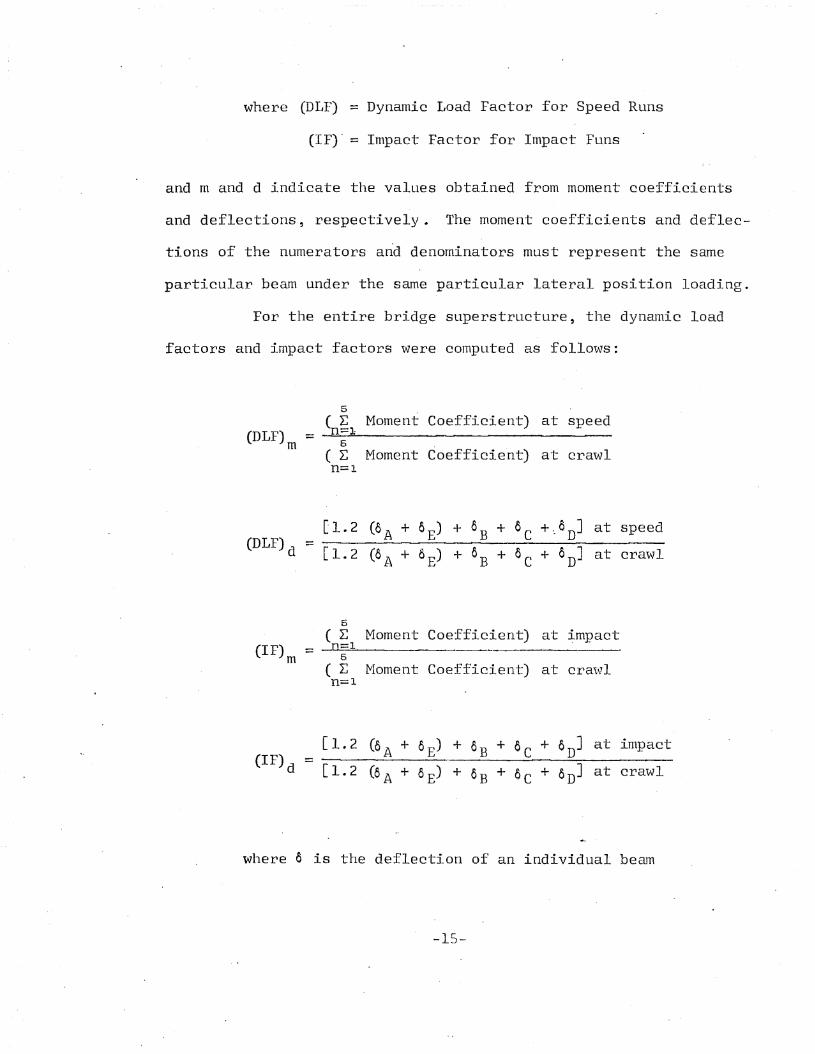
For the entire bridge superstructure, the dynamic load
factors and impact factors were computed as follows:
5
~~J. Moment Coefficient) at speed(DLF) =m 5
Coefficient)( E Moment at crawln=l
(DLF) d =[1.2 (oA + 0E) + 0B + 0c +coD] at speed
[1.2 (oA + 8E) + 0B + 0c + 0D] at crawl
6( I~ Moment Coefficient) at ~.mpact
(IF) ::: n=lm 5
( ~ IYloment Coefficient) at cra'\vln=l
(IF) d ==[1.2 ~A + 0E) + 0B + 0c + 0D] at impact
[1.2 (5 A + 5E) + 0B + 0c + 0D] at crawl
where a is the deflection of an individual beam
-15-
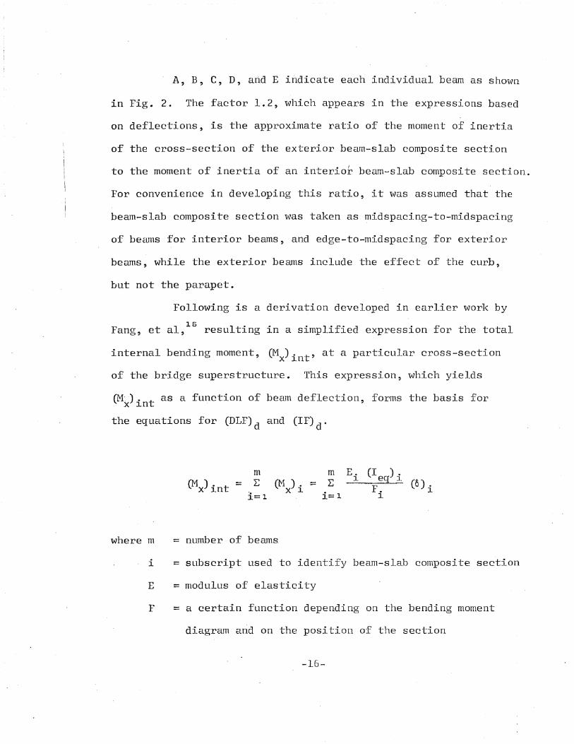
A, B, C, D, and E indicate each individual beam as shown
in Fig. 2. The factor 1.2, which appears in the expressions based
on deflections, is the approximate ratio of the moment of inertia
of the cross-section of the exterior beam-slab composite section
to the moment of inertia of an interior beam-slab composite section.
For convenience in developing this ratio, it was assumed that the
beam-slab composite seetioI1 was ta'ken as midspacing-to-midspacing
of beams for interior beams, and edge-to-midspacing for exterior
beams, while the exterior beams include the effect of the curb,
but not the parapet.
Following is a derivation developed in earlier work by
15Fang, et aI, resulting in a simplified expression for the total
internal bending moment, eM). t' at a particular cross-sectionx ln
of the bridge superstructure. This expre'ssion, which yields
(M:'). t as a function of beam deflection, forms the basis forx In
the equations for (DLF)d and (IF)d.
m~
1=1(M ). =
X 1
mI;
i= 1
where m
i
E
F
= number of beams.
= subscript used to identify beam-slab composite section
= modulus of elasticity
= a certain function depending on the bending moment
diagram and on the position of the section
-16-
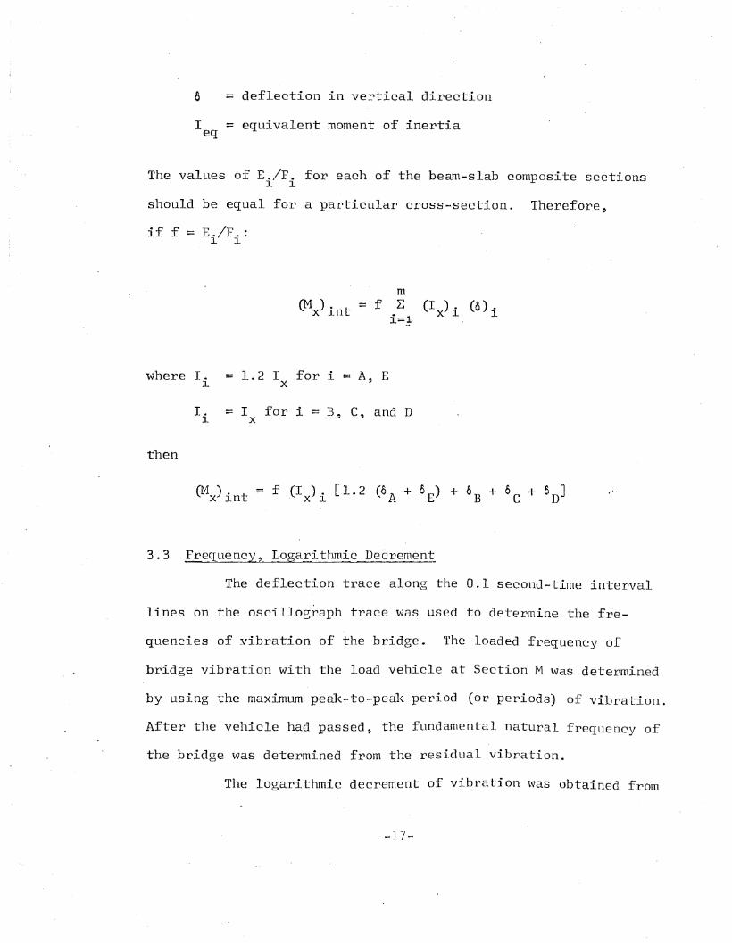
6 = deflection in vertical direction
I = equivalent moment of inertiaeq
The values of E./F. for each of the beam-slab composite sections1 1
should be equal for a particular cross-section. Therefore,
if f = E./F. :1 1
mE
i=:~·,
(I ). (6).x 1 1
where Ii = 1.2 Ix for i = A, E
I. = I for i = B, C, and D1 X
then
3.3 Frequency, Logarithmic Decremen~
The deflection. trace along the 0.1 second-time interval
lines on the oscillograph trace was used to determine the fre-
quencies of yibration of the bridge. The loaded frequency of
bridge vibration with the load vehicle at Section M was determined
by using the maximum peak-to-peak period (or periods) of vibration.
After the vehicle had passed, the fundamental natural frequency of
the bridge was determined from the residual vibration.
The logarithmic decrement of vibra ti.on \vas obtained from
-17-
selected runs by scaling the decreasing amplitudes of successive
decaying cycles of residual vibration, where
logarithmic decrementA
_ 1 log ~n A
n
n = the number of cycles of vibration
AAO = the amplitude ratio of the first to the nth cycle
n
-18-
4.· THE COMPUTATION OF MOMENT COEFFICIENTS
Two d'ifferent methods, which have been utilized. in the
previous work, were used to obtain the moment coefficients in
this study. The first method was used in the work presented in
3 4 5 6 7 8Reports Nos. 315.1 , 315.2 , 315.4 , 315.5 , 315.6 ,'and 315.7 ..
On the other hand, the second method was first used by M. A.T . T 16
Macias-Rendon, as outlined in Report No. 322.1.
In this study certain assumptions were utilized. With
the linear strain distributions, neutral axes, and the dimensions
of the cross-sections, two separate Fortran IV computer programs
were developed for these two methods.
4.1 The First Method
4.1.1 Linear Strain Distribution
From the previous studies, it was consistently demon-
strated that the linear strain distribution of the beam-slab unit
extended up through the curb section for the exterior beam.
Figure 5 shows the plots of the strains along the side faces of
interior7
and exterior beams of the Philadelphia Bridge, indicat-
ing that full composite ~ction existed between the beam, slab, and
curb. The dimensions of the cross-section of the Philadelphia
Bridge are essentially the same as those of the Hazleton Bridge,
and the test spans differ by 26 inches. Therefore, since it was
believed that the linear strain distribution would extend through
-19-
the slab and curb in the Hazleton Bridge~ no longitudinal gages
were placed on the surfaces of the curb and slab in the vicinity
of the exterior beam.
4.1.2 Consideration of Parapet
Figure 5 indicates that in the Philadelphia Bridge, the
linear strain relationship extended only up through the curb' sec-
tion, while relatively low strains were found in the parapets.\
Therefore, in this .report, the effect of the parapets was neglected
in the computations.
4.1.3 Use of Symmetry and Superposition
Since the cross-section of the bridge superstructure was
symmetric, only Beams A, B, and C were gaged. The moment coeffi--
cients for Beams D and E were then taken -as the values from Beams
A and B, when the vehicle was located in a symmetrical test lane
on the opposite side of the bridge. For instance, the moment
coefficients in Beams C, D, and E with vehicle running in Test
Lane 3 were considered to be equivalent to the moment coeffi-
cients in Beams C, B, and A, respectively, with the vehicle run-
ning in Test Lane 5. The use of symmetry and superposition was. 4
verified in the Drehersville Bridge study conducted in 1964.
4.1.4 The Modular Ratio
Since the moduli of elasticity of concrete for beam,
slab, and curb were unknown, the actual ratio of the elastic
-20-
modulus of the slab or curb concrete to that of the beam concrete
· 1· 1 d 10.could not be obtained. In an earller ana ytlca stu y, It was
shown that the variation of the modular ratio would not cause
significant changes in the section modulus and the moment of
inertia of the beam-slab unit. Therefore, in this study, 0.8 was
used as the value for the modular ratio in all computations.
4.1.5 Linear Variation of Slab Strains
Since no longitudinal strain gages were placed on the
slab, it was assumed that the longitudinal slab strains varied
linearly over the width of slab which acted compositely with each
beam.
4.1.6 Support Restraints
In line with previous field studies on this project, it
was assumed that longitudinal restraint produced by the end sup-
ports was negligible.
4.1.7 Effective Slab Widths'
Since the longitudinal restraining force in the members
was -neglected, the compressive force on the cross-section was com-
puted to be equal to the tensile force. Based on this point, the
effective wid~h of slab (and curb for the exterior beams) of an
individual beam-slab unit was calculated by the transformed sec-
tion method, equating the first moments of the compression area
and the tension area with respect to the measured location of the
neutral axis.
-21-
. .
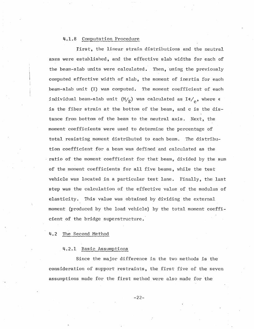
4.1.8 Computation Procedure
First, the linear strain distributions and the neutral
axes were established, and the effective slab widths for each of
the beam-slab units were calculated. Then, 'using the previously
computed effective width of slab, the moment of inertia for each
beam-slab unit (I) was computed. The moment coefficient of each
individual beam-slab unit (M/E) was calculated as Ie/c ' where €
is the fiber strain at the bottom of the beam, and c is the dis
tance from bottom of the beam to the neutral axis. Next,_ the
moment coefficients were used to determine the percentage of
total resisting moment distributed to each beam. The distribu
tion ,coefficient for a beam was defined and calculated as the
ratio of the moment coefficient for that beam" divided by the sum
of the moment coefficients for all five beams, while the test
vehicle was located in a particular test lane. Finally, the last
step was the calculation of the effective value of the modulus of
elasticity. This value was obtained by dividing the external
moment (produced by the load vehicle) by the total moment coeffi
cient of the bridge superstructure.
4.2 The Second Method
4.2.1 Basic Assumptions
Since the major difference in the two methods is the
consideration of support restraints, the first five of the seven
assumptions made for the first method were also made for the
-22-
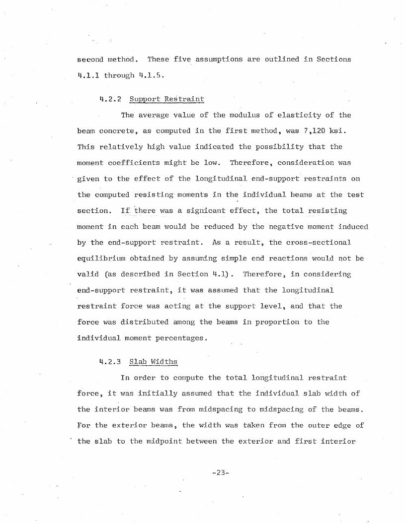
second method. These five assumptions are outlined in Sections
4.1.1 through 4.1.5.
4.2.2 Support Restraint
The average value of the modulus of elasticity of the
beam concrete, as computed in the first method, was 7,120 ksi.
This relatively high value indicated the possibility that the
moment coefficients might be low. Therefore, consideration was
given to the effect of the longitud~nal end-support' restraints on
the computed resisting moments in the individual beams at the ,test
section. If ~here was a signicant effect, the total resisting
moment in each beam would be reduced by the negative moment induced
by the end-support restraint. As a result, the cross-sectional
equilibriL@ obtained by assuming simple end,reactions would not be
valid (as described in Section 4.1). Therefore, in considering
end-support restraint, it was assumed that the longitudinal
restraint force was acting at the support level, and that the
. force was distributed among the beams in proportion to the
individual moment percentages.
4.2.3 Slab Widths
In order to compute the total longitudinal restraint
force, it was initially assumed that the individual slab width of
the interior beams was from midspacing to midspacing of the beruns.
for the exterior beams, the width was taken from the outer edge of
~ the slab to the midpoint between the exterior and first interior
-23-
4.2.4
1.
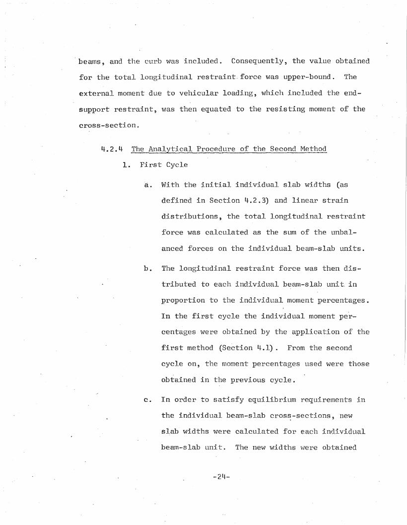
beams, and the curb was included. Consequently, the value obtained
for the total longitudinal restraint. force was upper-bound. The
external moment due to vehicular loading, which included the end
support restraint, was then equated to the resisting moment of the
cross-section.
The Analytical Procedure of the Second Method
First Cycle
a. With the ~nitial individual slab widths (as
defined in Section 4.2.3) and linear strain
distributions, the total longitudinal restraint
force was calculated as the sum of the unbal
anced forces on the individual beam-slab units.
b. The longitudinal restraint force was then dis
tributed to each individual beam--slab unit" in
proportion to the individual moment percentages.
In the first cycle the individual moment per
centages were obtained by the application of the
first method (Section 4.1). From the second
cycle on, the moment percentages used were those
obtained in the previous cycle.
c. In order to satisfy equilibrium requirements in
the individual beam-slab cros~-sections, new
slab' widths were calculated for each individual
beam-slab unit. The new widths were obtained
-24-
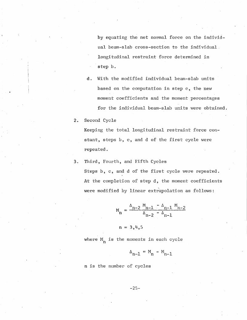
by equating the net normal force on the individ-
ual beam-slab cross-section to the individual,
longitudinal restraint force determined in
step b.
d. With the modified individual beam-slab units
based on the computation in step c, the new
moment coefficients and the moment percentages
for the individu'al beam-s lab units were obtained'.
2. Second Cycle
Keeping the total longitudinal restraint force con-
stant, steps b, c, and d of the first cycle were
repeated.
3. Third, Fourth, and Fifth Cycles
Steps b, c, and d of the first cycle were repeated.
At the completion of step d, the moment coefficients
were modified by linear extrapolation as follows:
n = 3,4,5
where M is the mome11ts in each cyclen
6 1 = Mn- n
n is the number of cycles
-25-
Mn-l
It was found that the moment coefficient converged
very rapidly. Within five cycles the moment per
centages obtained were in good correlation with the
field measurements.
4. The experimental modulus of elasticity of the bridge
superstructure was derived by dividing the sum of
the moment coefficients into the total moment pro
duced by the load vehicle at the maximum moment
section.
-26-
s. PRESENTATION OF TEST RESULTS
5.1 General
The results presented are based on the data obtained
from the longitudinal gag~s and deflection gages located at the
maximum moment section, Section M. The results from the trans
verse gages and reinforcement gages are not included. Since two
methods were used to obtain the moment coefficients, for conveni
ence, the first method is called Case I, and the second method,
Case II. Therefore, in the tables and figures, the numerical
values and the curves are labeled as Case I or Case II. The
number of the test ·lane and vehicle speed are indicated, where
needed.
5.2 Moment Coefficients, Elastic Modulus
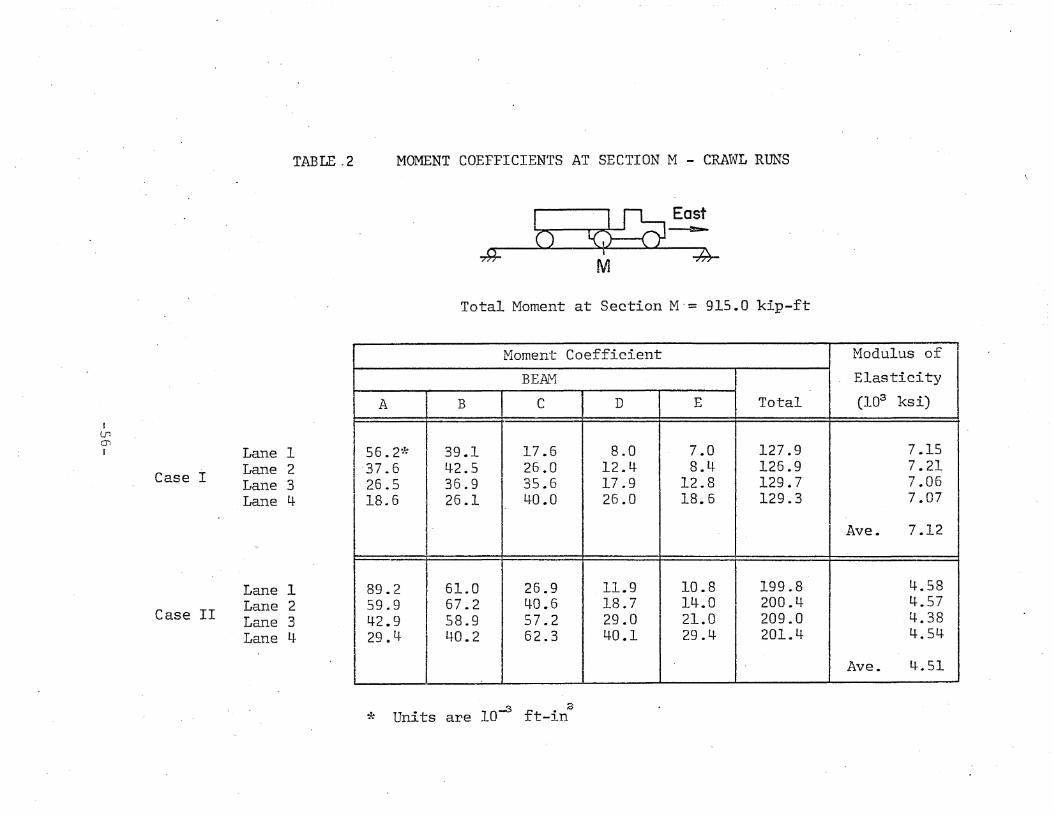
The computed moment coefficients, presented in Tables
2 through 7, reflect the magnitude of the bending moment in each
beam produced by the load vehicle at Section M when the vehicle
is traveling in the designated test lane and at the indicated
speed. Table 2 gives the average values of the moment coeffi
cients for crawl runs obtained from three different runs per
lane. Tables 3, 4, 5, and 6 give the moment coefficients for
Case I and Case II for speed runs on Test Lanes 3 and 4, and
Table 7 gives the moment coefficients for impact runs.
Table 2 also gives the experimental value of the
-27-
modulus of elasticity. The average experimental value of the
modulus of elasticity of the beam concrete was computed to be
7,120 ksi and 4,510 ksi for Case I and Case II, respectively.
5.3 Distribution Coefficients
Distribution coefficients, which are defined as the
percentages of total vehicle moment distributed to individual
beams" are presented in Tables 8 through 11. For crawl runs,
the average values from three sets of test runs were used.
Figures 6 through 13 illustrate the variation in the distribu
tion coefficients for crawl and impact runs, for Cases I and II.
5.4 Distribution Influence Lines and Distribution Factors
In Figs. 14, IS, and 16, the influence lines for the
distribution coefficients are plotted for Beams A, B, and C with
the vehicle in various load lanes. All distribution coefficients
are based on crawl runs. The base line of the diagram corres
ponds· to the lateral location of the center of the test vehicle
on the bridge roadway. The top line of the diagram indicates the
bounds of the design traffic lanes. Since the distribution co
efficients obtained' from Case I and Case II were very close, only
one line is actually shown, although points representing both
Cases I and II are plotted.
To develop experimental distribution factors, a design
load vehicle was placed in each of the three traffic design lanes,
as explained in Section 3.2.3. The width of the design traffib
-28-
lanes for this bridge was 13 feet 4 inches, the center-to-center
width of the design load vehicle wheels is 6 feet, and the minimum
distance from the center-line of the wheels on one side of the
vehicle to the curb face, or to the edge of the lane, is 2 feet.
Therefore, to maximize the effects, the center-line of the truck
can be placed at any location within the middle 3 feet 4 inches
of each design lane. Table 12 shows the development of the
experimental distribution factors through use of the influence
lines (Figs. 14-16). The experimental distribution factor for
a particular beam was obtained by summing the three maximum dis
tribution coefficients from each design lane, and multiplying the
total by two since distribution factors are to be applied ,to wheel
loads rath~r than axle loads. Figure 17 shows a graphical compari
son between the distribution factors actually used in design of
the different beams, and the "experimentally developed distribution
factors.
5.5 Deflections and Deflection Influence Lines
Beam deflections at Section M, listed in Tables 13, 14,
and 15, were directly calculated f~om oscillograph recordings.
For the crawl runs, average values of three sets of test runs were
used. To enable an evaluation of~the vertical deflection charac
teristics of individual beams, the influence lines for deflections
from the crawl runs are given in Fig. 18. In the figure, the
ordinate represents the vertical deflection of a ,particular beam,
-29-
while the base line and the top line correspond to the lateral
location of the test lanes and the design lanes, respectively.
Figure 19 shows the maximum individual beam deflections produced
by the individual maximuln loading caridi tions.
5.6 pynamic Load Fac~ors and Impact Factors
The dynamic load factors listed in Tables 3, 4, 5, and
6 were calculated as explained in Section 3.2.5. These tables
present the dynamic load factors for individual bemfis, and for
the over-all bridge behavior, with the t~st vehicle in a parti
cular test lane traveling at various speeds. These factors are
based on moment coefficients, while the dynamic load factors
based on deflections are given in Tables 14 and 15. Tables 16
and 17 list the dynamic load factors derived from the impact
runs. Table 18 lists the dynamic load factors for the total
bridge" behavior with th~ test vehicle in Test Lanes 3 and 4 at
vario~s speeds. The values for (DLF)m were computed utilizing
the methods of both Cases I and II. Figures 20, 21, and 22 show
the variation in the dynamic load factors for the individual
beams as a function of vehicl~e speed, for t-he test vehicle in
Test Lane 4. These figures were based on the moment coefficients
obtained from Case I (Fig. 20), the moment coefficients obtained
from Case II (Fig. 21) and deflections (Fig. 22). Figures 23,
24, and 2S similarly show the dynamic load factors for the total
bridge as a function of vehicle speed.
-30-
5.7 . Neutral Axes
Tables 19, 20, and 21 list the locations of the neutral
axes, described by the distances from the bottom face of the.beam
to the location of the neutral axis art the left and right vertical
faces. Table 19 lists the location of the neutral axis for crawl
runs and impact runs. The location for crawl runs was obtained
by averaging the values of similar test runs. Tables 20 and 21
list the values for the various speeds while the test vehicle ran
in Test Lanes 3 and 4, respectively. Figure 26 shows the typical
neutral axis location for crawl runs in the various test lanes.
5.8 Effective Slab Widths
Table' 22 lists the effective slab widths for each bewl,
as determined for crawl and impact runs. As before, the crawl
run values represent the averages from three similar test runs.
Table 23 gives' the total effective slab width for Cases I and II,
with the test vehicle traveling in Test Lanes 3 and 4 at various
speeds. Table 24 lists effective slab widths for each beam for
Cases I and II, while the test vehicle is traveling at various
speeds in Test Lanes 3 and 4. Since there were no limitations
imposed' in calculating the effective slab width in both, the
effective slab width of the exterior beam and the interior beam
could exceed 102 or 114 inches, respectively. Similarly, total'
effective slab width might be over the total slab width of 546
inches, . the width of the bridge. This overlapping ?f compression
zones gave an upper bound solution.
-31-
,5 • 9 Freguencies
All frequencies of bridge vibration were obtained from
the oscillograph traces of the three beam deflection gages.
Since the entire bridge would vibrate under the vehicular loading,
the frequencies of each beam should be equal to each other when
the vehicle was loaded on a particular test lane. Therefore, the
average values of these frequencies were obtained from three
deflection gages. As a matter of fact~ oscillographic recordings
showed that these three values were almost identical.
The fundamental unloaded natural frequency of the
Hazleton Bridge computed as the average value from 40 test runs,
was 5.75 cps. Table 2S lists the loaded frequencies of bridge
vibration with test vehicle in each particular test lane for
impact runs. Table 26 lists the loaded frequencies of bridge'
vibration with the test vehicle in Test Lanes 3, 4, and 5. In
order to co.mparethe dynamic load factors with the test vehicle
in Test Lane 3, the average frequency of the loaded frequencies
under the test vehicle ~n Test Lane 3 and 5 were calculated.
Figure 27 shows the loaded frequencies of bridge vibration as'-
a function of vehicle speed.
5~lO Logarithmic Decrement
, The logarithmic decrement of vibration to study the
.damping characteristic of the bridge was obtained from the oscil-
· lograph trace of three beam deflection gages on three speed runs.
-32-
To gather the needed data, the oscillograph records were left
running after the vehicle had completed its passage. Table 27
lists the logarithmic decrement value obtained from these three
runs.
-33-
6. DISCUSSION OF RESULTS
6.1 Static Live Load Effect
To simulate the static live loading condition, crawl
runs were used.
6.1.1 Distribution Factors
One of the main objectives of this study was to evaluate'
the distribution factors for 'individual beams. ',Comparison of
design and experimental distribution factors indicated that the
design value for interior beams is significantly greater than the
experimental value (Table 12 and ,Figure I?), whereas, the design
value for exterior beams is somew4at less than that of the experi
mental value. Therefore, it can be concluded that the design
value for interior beams was considerably over-conservative. How
ever, since the exterior beams were carrY,ing n10re moment than tIle
design load, it should not be concluded that the exterior beams
were under-designed •. The development of full composite action
between the curb and the beams, and the partj_al composite action
between the parapet and t~e curb, increased the flexural stiff
ness of the exterior beams. ConsequentJ_y, the maximw"n flexural
~ stress produced in the exterior beams was reduced.
Effect of the cross-sectional properties can be examined
by comparing the results of the Drehersville, Philadelphia and
Hazleton bridges, which consist of five identical ,beams ea~h;
-34-
The dimensions and comparison of distribution factors for these
three bridges are shown in Table 28. The major difference in
terms of the outlay of the bridges was the numer of design traffic
lanes. Drehersville Bridge was designed for two lanes, whereas,
Hazleton and Philadelphia bridges were designed for three lanes.
All cross section dimensions of the Philadelphia and Hazleton
bridges were the same except for a 2 foot, 2 inch difference in
span length. Consequently the experimental· distribution factors
for the Philadelphia and Hazleton Bridges are almost identical.
However, due to the dissimilar geometry, the Drehersville Bridge's
distribution factors are substantially different from those of
the Hazleton and Philadelphia Bridges. The ratio of the experi
mental distribution factor to the design distribution factor for
the exterior beam of the Drehersville Bridge is larger than that
of the Philadelphia and Hazleton Bridges. This indicated the high
experimental to design distribution factor ratio for exterior
beams of bridges with closely spaced beams. In the design, con
tribution of the curb and parapet by_!?e full and/or partial com
posite action was not considered. However, field study concl~ded
the existence of such interaction (Section 4.1.~ 0 Reconsidera
tion of the high experimental to design distribution factor ratio
for closely spaced beams indicated the pronounced effect of the
curb and parapet to the stiffness of exterior be~ls, for these
types of bridges.
The above co~parisons yield that the distribution
-35-
factors not only depend on the beam spacing and cross-sectional
properties but also on the span length of the beam, the number of
traffic lanes, and the interaction of curb .and parapet. Since the
current design method does not reflect the influence of beam'
spacing, it is not realistic enough.
The method to determine the distribution factors pro
posed by W. W. Sanders, Jr. and H. A. Elleby17 considered the
cross-sectional property, the beam span and the total number of
design traffic lanes. It also suggested the use of the same dis-
tribution factor for all beams, both interior and exterior. How-
ever, the Sanders and Elleby study did not include the effects of
curb and parapet section. The method suggested by Mot~rjemilO
took the roadway width, the number of design traffic lanes, the ~
number of beams,_beam spacing, and the span length into account.',
for the dist~ibution factor of interior beams. His approach also
excluded the effect of curb and parapets. Observations based on
field testing of the Hazleton Bridge, as well as previously con-4 7 ;
ducted and reported re~earch ~ conclusively showed necessity of
the inclusion of the composite effect of the curb in the design
and the analysis of bridge response.
6.1.2 Beam Deflection
Measured beam deflections were quite small, as can be
noted in Table 13. The maximum beam deflection measured at maxi-
mum moment section' was only 0 .108 inches. TIle maximunt vertical
-36-
deflection under three vehicle loading could be 0.198 inches for
the center beam and 0.169 inches for the exterior beam (Figure 19) .
6.1.3 Neutral Axes
Figure 26 shows typical examples of neutral axis· loca-
tion for various lane loading~. The neutral axis of the beam
tended to incline when the vehicular loading was not applied
directly above the beam. The inclination of the neutral axis
indicated the biaxial bending of the beams. In general, the
vertical location of the neutral axis with respect to the bottom
beam face was highest when the 'test vehicle was positioned di-
rectly above the beam, and progressively lower as the test
vehicle foilowed a path farther away from the beam axis.
6.2 Moving Load Effect
6.2.1 Moment Coefficients
As shown in Tables 3, 4, 5,. and 6, the moment coeffi-
cients for each individual beam and total bridge response' ampli-
fied with speed in an inconsistent pattern. The moment coeffi-
cients for ,individual beams and the total bridge response reached
the maximum at about the vehicular speed of 26 mph.
In Figures 28, 29, 30, and 31, the moment coefficients
were plotted along with curves that represent the crawl run
50results multiplied by the factor (1 + L + 125). Whereas, for the
beam'with small moment coefficient, the experimental nl0ment
-37-
coefficient for speed runs was sometimes larger than the value
suggested by AASHO. Nevertheless, this should not be interpreted
as to the use of factor (1 + L ~0125)' which may lead to under
design~ For one vehicle loading, the moment coefficient may ex
ceed the specified value. However, for simultaneous loading by
two or more vehicles, the different forcing functions would have
a balancing effect.
6.2.2 Distribution Coefficients
Different vehicular speeds resulted in different dis
tribution coefficients. Variation in the distribution coeffi-
cients with respect to vehicular speed was marginal. The in
creased vehicular speed provided more uniform·distribution of
the vehicular load among the beams.
6.2.3 Dynamic Load Factors
Amplification of the static response of the individual
beams was not linearly related to the vehicular speed (Figures
20, 21, 22). The dynamic response of the individual beams was
quite similar up to 20 mph. From this speed on, their response
was very dissimilar. In beams with small moment coefficient
(Beam A in Figure 20, 21, 22), the dynamic load factor was
larger than the value recommended by the specifications. 1 Where
as, in beams with large moment coefficient (Beam C in Figures 20,
21, 22) the dynamic load factor was less than the recommended
value and close to 1.00. The same pattern was observed in the
-38-
moment coefficients and the distribution coefficients. This indi-
cated that the lateral load distribution for speed runs above
20 mph is more nearly uniform than that for crawl runs.
The study of the total bridge response with respect to
varying vehicular speed was made. Variation of the dynamic lead
. factor for gradually increasing speed obtained by different
approaches. Figures 23, 24, and 25 reaffirmed the lack of any
linear relation between the cause and the effect. A careful
examination of these relations indicated existence of maximum
dynamic load factor at 26 mph vehicle speed; and there was a
secondary peak of dynamic load at approximately 55 mph. The
source of this phenomenon will be explained in Section 6.2.4.
The magnitude of dynamic load factor for total bridge
behavior under one vehicle loading was, for certain speeds,
larger than the impact-factor suggested by- AASHO. This was
particularly noticeable at the maximum and the secondary peaks.
6.2.4 Frequencies
The experimental unloaded. frequency of the Hazleton
Bridge was 5. 7S cycles per second. This value can· 'be compared
with the theoretical natural frequency, which was based on the
first mode of vibration of a simple-supported beam of uniform
cross-section and mass per unit length. The theoretical natural
frequency is given by:
TT IfTmIf=--2 '\1m2L
-39-
where L ...... span of the bridge
E ;:: modulus of elasticity of beam concrete
I ::: moment·of inertia of tIle bridge cross-section
m = mass per unit length of the bridge
The modulus of elas~icity of concrete was obtained as
7.12 x 10⁶
psi and 4.51 x 10⁶
psi from Case I and Case II, res-
pec~ively. In computing the moment of inertia of the bridge ratio
of slab to beam, modulus of elasticity was taken as .8. In the
computation: of the moment of inertia the parapets were not taken
into account. The natural frequency equation yield 6.48 cps and
5.16 cps for Case I and Case II, respectively. There was a 10%
difference between the experimental frequency and the theoretical
frequency of 5.16 (Case II). If the modulus of elasticity of con-
crete should have" been taken as somehow higher than the value of
4.51 x 10⁶
psi and if the partial effect of the bridge parapet
was considered for moment of inertia of the bridge, than the theo-
retical value would have been closer to the experimental value.
These two suggested modifipations have practical relevance. It
can safely be assumed that tl1e modulus of elastici-ty of the bridge6
superstructure was higher than 4.51 x 10 psi (Section 6.4.3) .
Also, the partial composite interaction of the parapet exists.
The use of the theoretical formula introduces a certain systematic
error. The forrnllia is for simple beam resting on two roller
supports. Whereas, the bridge supports were 9 inches wide bearing
pads, rather than rollers.
.... 40-
12Biggs, Suer, and Louw suggested the expression
f =
for unloaded natural frequency. If the previous values were mul-
tiplied by the, factor of 1.2, it would be 7.78 cps and 6.19 cps·
for Case I and Case II, respectively. Both new values were higher
than the experimental values. The over-estimation of the fre-
quency could be found in the development of the suggested expres-
sian. The study by Biggs, Suer, and Louw was based on the re-
sponse of steel bridges. Thus, it can fundamentally be assumed
that the reinforced concrete beam-slab type bridge can be simu-
lated by a simple beam of uniform cross-section.
Study of the dynamic response characteristics of the
bridge (Figs. 23, 24, and 25) indicates the presence of maximums
in the dynamic load factor versus the speed relations. At the
speed of about 26 mph and 5S mph the bridge was subjected to
higher dynamic loads as compared to other speeds. The cause of
these can be explained if the natur~l and the loaded frequencies
are studied. The vehicle of constant weight and variable speed
can be considered as a harmonic forcing function. The variation
in the speed of tpe 'vehicle can be interpreted as the variation
in the harmonici ty of the forcing function. Thus, arourld certain
quasi-critical speeds of the vehicle, the natural frequency of
the bridge will be close to the forcing frequency (Fig. 27).
--41-
This, then, results in a large displacement.
11Linger and Hulsbos reported a different approach. The
axle load of the vehicle was simulated by a moving cyclial force
with variable forcing frequency. The resonance was predicted when
the forcing frequency became equal to the natural frequency of the
bridge. .Ho,\vever, the numerical treatment of the loaded ,fre,quency
could not be found in this study. According to Linger and
11Hulsbos, the loaded frequency was very close to the natural fre-
quency'. According to this report, the test' vehicle wouJ_d have
forcing frequency of v/13.0 and v/20.4 based on tractor wheel base~·
respectively; wher~ v is the vehicular speed (feet per second) •
6.2.5 Damving Effect
The logarithmic decrements are different for different
beams, and they a~e dependent on the lane of loading (Table "27) .18
This is in accord with the observations reported by Varney. The
logaritrunic decrements for the Hazleton Bridge ranged from 0.1028
to 0.1213 and were somewhat larger than previously reported11 18
values.' It can be stated that the damping characteristics of
the bridge lie somewhere between those given for flexible and for
stiff cOJnposite steel bridges wi th spar18 of about the same length
~s described by Kinnier and McKeel.19
6.2.6 Neutral Axes
The location of neutral axes of each individual beam
did not change significantly with respect to various speeds
-l~2-
(Tables·20, 21). This indicated that neutral axes are relatively
insensitive to the variation of vehicular speed.
6.3 Impact Loading Effect
6.3.1 Distribution Coefficients
Comparisons between the distribution coefficients for
impact runs and crawl runs were made (Figs. 32 through 35) .
Since, there were minor differences between the distribution
coefficients obtained in Case I and Case II; only Case II co
efficients were considered. Comparisons showed that distribution
coefficient changes, for impact runs, were heavily dependent upon
which lane. was loaded. There were significant differences between
crawl and impact run dist~ibution coefficients when the vehicle
was above or near the exterior beam (Figs. 32, 33). Whereas, for
the runs· above or near the center beam, the variation in the crawl
and impact distribution coefficients was marginal. Furthermore,
the lateral distribution of the impac~, loads was consistently
smoother when compared to the static distribution.
6.3.2 Moment Coefficients and Impact Factors
·Since the moment coefficients obtained in Case I and
Case II for crawl runs were different, moment coefficients for the
impact runs were compared with Case I and II values (Figs. 36
through 39). The moment coefficients of .individual beams for
impact runs were larger. than those for crawl runs in both cases.
-43-
T11e impact factors for individual beams range from 1.5 to 5.0 or
more (Table 16). The impact factors for the total bridge be
havior, regardless of the position of the vehicle, were 2.00,
2.35, and 2.15, based on the moment coefficients of Case I, the
moment coefficients of Case II, and deflections, respectively.
Thus, under impact loading, the crawl run response of the bridge
was amplified by the factor of two.
6.3.3 Neutral Axes
The location of the neutral axes of each beam for
various lanes of impact runs (Table 19) were relatively lower than
that for crawl runs. Consequently, the 'total effective slab
widths for impact runs were less than that of crawl runs in
Case I (Table 22).
6.4 End Restraint Effect
In this study, two methods were utilized to compute
moment coefficients; the first method (Case I) did not include the
longitudinal restraint, whereas the second method (Case II) did.
The effects of inclusion of the ,end "restraint are presented in
Sections 6.4.1 through 6.4.5.
6.4.1 Distribution Coefficients
Inclusion of the end restraints had practically no
effect on the distribution coefficients. This indicates that the
two methods would yield almost the same results for the
-q4 ....
experimental distribution coefficients.and the experimental dis~
tribution factors.
6.4.2 Moment Coefficients
In Case I,·as explained in Section 4.1.6, the external
moment due to the vehicle was assumed to be equal to the internal
bending moment of the bridge superstructure. In Case II, as
explained in Section L~.~.2, the external moment due to the
vehicle was assumed to be equal to the sum of the internal bending
moment and the moment due to the longitudinal restraint force.
Consequently, the moment coefficient obtained from Case II would
be larger than that from Case I. The degree of difference between
the two moment coefficients depends on the magnitude of the end
restraint force.
6.4.3 Modulus of ~lasticity
The experimental elastic modulus of concrete of the
superstructure was obtained froln the relations established between
the external moment and the. total moment coefficients~ Since
there were two moment coefficients,.Case I and Case II, two values6
of elastic moduli were obtained, i.e., 7.12 x,lO psi for Case I,
6 204.51 x 10 psi for Case II. According to ACI Code and PCl
2L h 1 fl· fCode, t e modLl us a e astlci ty or concrete is tal<.en as
E Wl.5 33~.fTand E -- 1,800,00 50 fT= vI' + 0 , respectively, wherec c c c
W is the weight of concrete in pounds per ft., and £1 is the come
pressive strength of concrete in psi. The specified minimum
28-days cyclinder strength of the beam concrete was 5500 psi. If
fT should have reached 6000 psi at the time of the field testingc
of the bridge, then E would be 4.45 x 10⁶
psi and 4.8 x 10⁶
psi,C
in accordance with ACI and ·PCI Codes, respectively. If f1 shouldC
have reached 7000 psi, then E . would be 4.8 x 10⁶
psi andc
5.3 x 10⁶
psi. Regardless of the choice of code, ACI or PCl, and
of the concrete strength, 6000 psi or 7000 psi, the predicted
modulus of elasticity is close to the one obtained in Case II.
6.4.4 Dynamic Load Factors and Impact Factors
In the analysis of the dynamic behavior of the bridge,
inclusion or exclusion of the end restraint effect would still
result in similar response predi~tions (Figs. 20 through 25).
Nevertheless, the magnitudes of these response predictions may
~iffer. Thus, two methods could obtain the same adequate results
for the analysis of dynamic effects. A careful examination of
the results by different approaches (Figs~ 20 through 25) shows
t,ha t the dynamic load factors and impact factors obtained from
Case I were closer to the value obtained from deflection than
that of Case II.
6.4.5 Effective Slab Widths
The total effective slab widths obtained from Case I
were less than 400 inches, while the total effective slab width
from Case II were around 540 inches (Tables 22, 23, 24); the
actual total slab width was 546 inches. Consequently, the moment
-46-

coefficients obtained from Case II were relatively larger than
those obtained from Case I.
-47-
7. S~1ARY AND CONCLUSIONS
7.1 Summ~ry
The major objectives of this study were to provide addi-
tional information on lateral load distribution for spread box-
beam slab type bridges under static vehicle loading, and to .experi-
mentally investigate the dynamic effects of moving vehicle loading
and vehicle impact loading. The report presents part of the
results, based on the data obtained in the field test of the
Hazleton Bridge.
The test bridge consisted of five identical precast pre-
stressed concrete box-beams with a composite cast-in-place rein-
forced concrete slab, and reinforced concrete curbs and parapets.
Beam strain gages and deflection meters were applied at the section.'.
where maxinlum moments occur. A truck simulating AASHO HS 20-44
loading was used as the test vehicle. Seven test lanes were
located on the roadway such that the center-line of the test
vehicle would coincide with the beam center-line or the center-
line of the beam spacing. 22 crawl, 73 speed, and 11 impact runs
by the test vehicle were conducted to generate the experimental
data. In the speed runs, the speed of the vehicle varied from
5 mph to 60 mph and in impact runs the test vehiclefs speed was
maintained at 10 mph.
Strains and deflections were reduced from the oscillo-
graph traces. Loaded frequencies and unloaded natural frequency
-48-
of the bridge were direc~ly measured fr01TI the oscillograph traces.
From the strains, the linear strain distribution and the
location of the neutral axes were obtained. The moment coeffi
cients, experimental live load moments, distribution coefficients
and effective slab widths were determined by using two different
methods, one excluded the end restraints, and the other considered
the end restraints. The experimental distribution factors were
computed from the distribution coefficient influence lines.
Experimentally obtained distribution factors were compared with
the design distribution factors and with the reported values for
the Drehersville and Philadelphia Bridges. The dynamic load
factors for speed runs and the impact factors for impact runs were
determined by two' different methods. They were taken as the ratio
between the moment coefficients or deflections of uynamic loading
(speed run and impact run) and the moment coefficients or deflec
tions of s~atic loading (crawl run). The loaded frequencies of
bridge vibration under various vehicle speeds were utilized to
find the vehicle speeds which may cause maximum dynamic response.
The experimental unloaded natural frequency was compared with the
theoretical value. Final comparison of the two methods, which
were utilized to obtain ~oment coefficients, was made.
7.2 Conclusions
Based on the field test results of the Hazleton Bridge
the following conclusions were reached:
-49-
3. The lateral load distributions for speed runs were
more· nearly uniform than of crawl runs. The lateral
load distribution for impact runs were significantly
more uniform than that of crawl runs.
4. The dynamic load factors for total bridge behavior
and for individual beam behavior were not linearly
related to the speed of the vehicle.
S. In the Hazleton Bridge, the peak dynamic response of
the-bridge occurred at a vehicle speed of 26 mph with
a dynamic load factor of 1.25 or more. There was a
secondary peak corresponding to a speed of approxi
mately 55 mph.
-50-
6. The experimental unloaded natural frequency of the
bridge has a good correlation with the theoretical
value, which was based on the first mode of vibration
of a simple-supported beam of uniform cross-section.
7. The maximum dynamic amplification of the bridge re
sponse was obtained when the observed loaded fre
quency of force vibration was approximately equal to
the natural unloaded frequency of the bridge.
8. The magnitude of dynamic amplification of bridge
response under impact loading (10 mph of speed and
2 inches drop) is t~ice as large as that under crawl
run loading (2.5 mp}l) .
9. Both methods used in this study to obtain moment
coefficients could be utilized to analyze the 's'truc
tural response of prestressed concrete box-beam
bridges. The first method neglected the restraint
effect of the end supports, and yielded the result-
ant moment actually p~oduced on the bridge cross
section. Whereas, the second method took the
restraint effect into consideratio~, and enabled the
calculation of the moment produced by the vehicle
loading only.
-51 ..~
8. ACKNOWLEDGMENTS
This st~dy presents partial results of Project 3lSA,
entitled "Structural Response of Prestressed Concrete Box-Beam
Bridges", conducted in the -Department of Civil Engineering at Fritz
Engineering Laboratory, Lehigh University, Bethlehem, Pennsylvania.
Dr. David A. VanHorn is Chairman of the Deparbnent and Dr. Lynn S.
Beedle is Director of the Laboratory. This project is sponsored
by the Pennsylvania Department of Transportation, the U. S. Bureau
of Public Roads, and the Reinforced Concrete Research Council.
The field test equipment was made available through the
cooperation of Mr. C. F. Scheffey, Chief, Structures and Applied
Mechanics Division, Office of Research and Development, Bureau of
Public Roads, U. S. Department of Transportation. The instrumen
tation and operation of test equipment were accomplished by Messrs.
R. F. Varney and H. Laatz of the Bureau of Public Roads. The basic
planning in this investigation was in~cooperation with Mr. K. H.
Jensen, formerly Bridge Engineer, and Mr. H. P. Koretzky, Engineer
in Charge of Prestressed Concrete Structures, both of the Bridge
Engineering Division, Pennsylvania Department of Transportation.
Dr. David A. VanHorn supervised the work of this thesis a
The writer owes him a sp~cial debt of gratitude fcir his advice,
critical review, and encouragement.
The writer wishes to express his deep appreciation for
. the advice and help of Dr. Celal N. Kostem, and thanks to Messrs.
-S2~
.Felix Barda and Chiou-horng Chen for their assistance.
Mrs. Ruth Grimes typed the manuscript- with patience and
willingness, and· Mrs. Sharon Balogh.prepared the drawings. Their
cooperation is appreciated.
-53-

g. TABLES
-Slt-
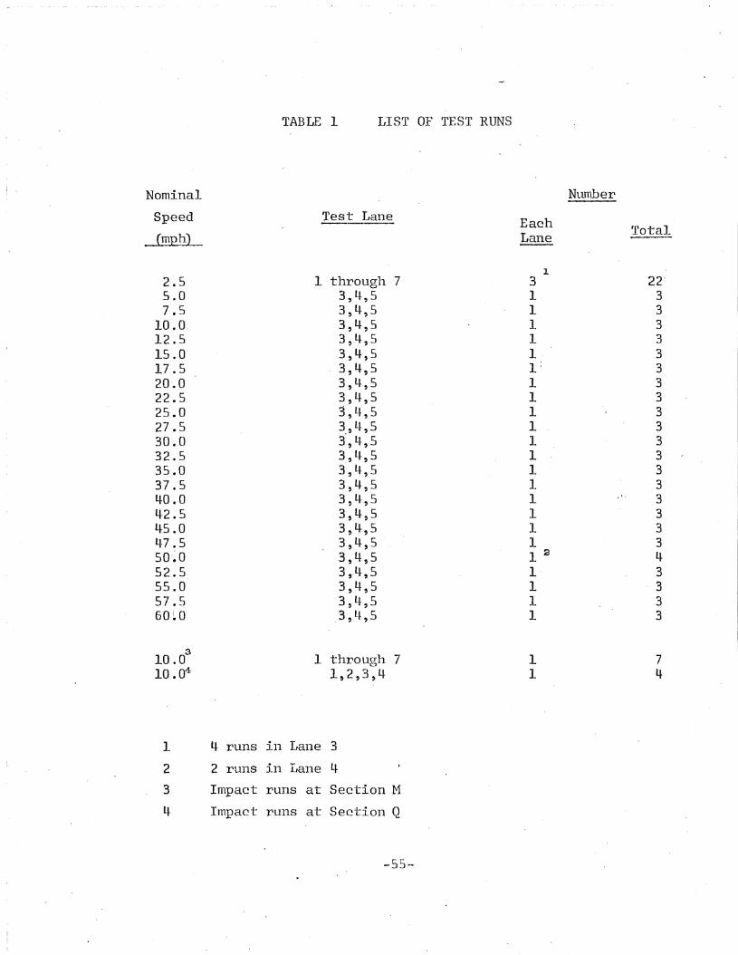
TABLE 1 LIST OF TEST RUNS
Nominal Number
Speed Test TJaneEach
~~ Lane 'fatal--"
12.5 1 through 7 3 22'5.0 3,L~,S 1 37.5 3,4,5 1 3
10.0 3,4,5 1 312.5 3,4,5 1 315.0 3,4,5 1 317.5 3,4,5 1.' 320.0 3,4,5 1 322.5 3,4,5 1 325.0 3,4,5 1 327.5 3" l~, 5 1 330.0 3,4,5 1 332.5 3,4)5 1 335.0 3,4,5 1 337.5 3,4,5 1 340.0 3,4,5 1 34-2.5 3,4,5 1 3L~S. 0 3,4,5 1 347.5 3,4,5 1 350'~O 3,4,5 1 a 452.5 3,.4,5 1, 355.0 3,4,5 1 357.5 3,4,5 1 360~O .3,4,5 1 3
310.0 1 through 7 1 710.04 1,2,3,4 1 4
1 4- runs in Lane 3
2 2 runs in Lane 4-
3 Impact runs at Section M
L~ Impact runs at Section Q
-55·..
IlJlmi
Case I
Case II
TABLE.2
Lane 1Lane 2Lane 3Lane 4
Lane 1Lane 2Lane 3Lane 1+
MOMENT COEFFICIENTS AT SECTION M - CRAWL RUNS
I ~._Easto ----.,g: IM .,4-
Total Moment at Section M-= 915.0 kip-ft
Moment Coefficient Modulus of
BEAM . Elasticity
A B C D E Total (103 ksi)
56.2* I 39.1 17.6 8.0 7.0 127.9 7.15·37 . 6 42.5 26.0 12.4- 8.4- 126.9 7.2126.5 36.9 35.6 17.9 12.8 129.7 7.0618 .. 6 26.1 40.0 26.0 18.6 129.3 7.07
Ave. 7.12
89.2 61.0 26.9 11.9 10.8 I 199.8 4.5859.9 67.2 4-0.6 18.7 14.0 200.4- 4.5742.9 58.9 57.2 29.0 21.0 209.0 4-.3829.4 40.2 62.3 40.1 29.4- 201.4- 4.54
Ave. 4 .. 51
* Units are 10-3 ft_in2
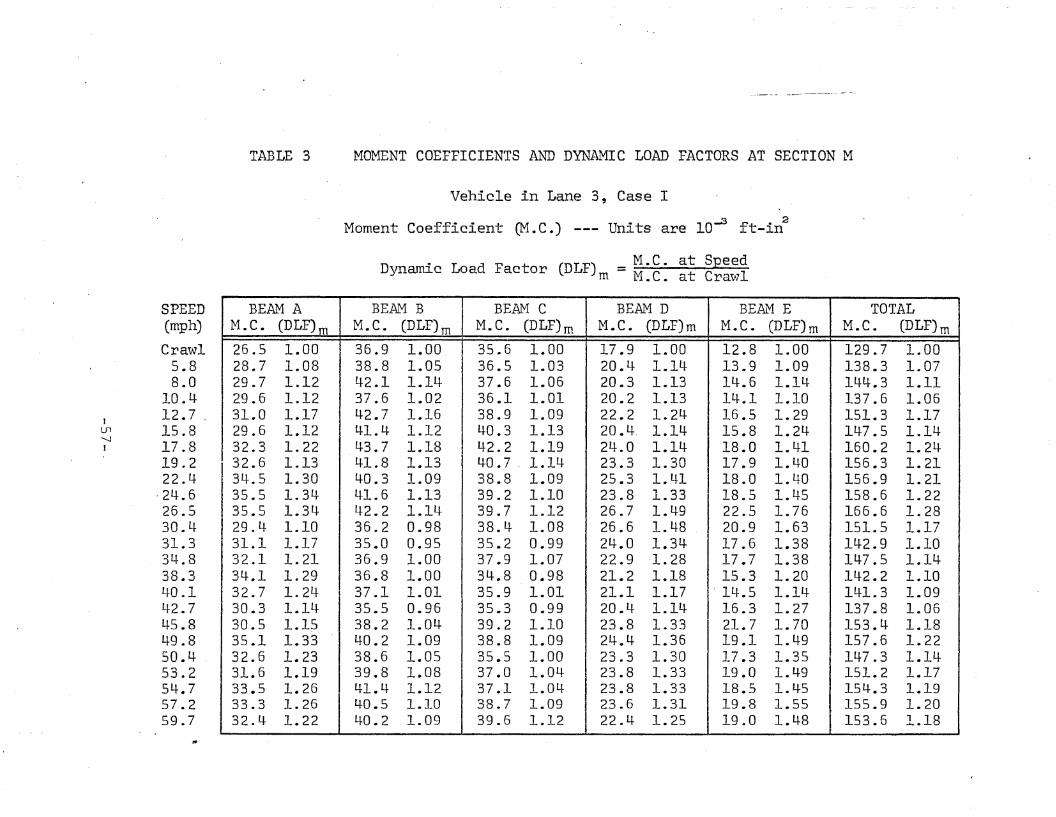
TABLE 3 MOMENT COEFFICIENTS AND DYNAMIC LOAD FACTORS AT SECTION M
Vehicle in Lane 3, Case I
Moment Coefficient (M.C.) --- Units are lO~ ft_in2
M.C. at SpeedDynamic Load Factor (DLF) m = M. C. at Craw·l
IU1-........JI
SPEED(mph)
Crawl5.88.0
10.412.7 .15.817.819.222.4-
·24.626.530.431.334.838.340.142.745.849.850.4 .53.254.757.259.7
..
BEAM A BEAM B BEAM C BEAM D BEAM E TOTALM. C. (DLF) m M. C. (DLF) m M. C. (DLF)m M.C. (DLF)m M.C. (DLF) m M.C. (DLF)m
26.5 1.00 36.9 1.00 35.6 1.00 17.9 1.00 12.8 1.00 129.7 1.0028.7 1.08 38.8 1.05 36.5 1.03 20.4 1.14- 13.9 1.09 138.3 1.0729.7 1.12 42.1 1.14- 37.6 1.06 20.3 1.13 14.6 1.14. 144-.3 1.1129.6 1.12 37.6 1.02 36.1 1.01 20.2 1.13 14.1 1.10 137.6 1.0631.0 1.17 42.7 1.16 38.9 1.09 22.2 1.24- 16.5 1.29 151.3 1.1729.6 1.12 41.4- 1.12 40.3 1.13 20.4-. 1.14- 15.8 1.24- 147.5 1.14-32.3 1.22 43.7 1.18 42.2 1.19 24.0 1.14- 18.0 1.41 160.2 1.24-
I 32. 6 1.13 41.8 1.13 40. 7 _ 1.14- 23.3 1.30 17.9 1.40 156.3 1.2134.5 1.30 40.3 1.09 38.8 1.09 25.3 1.41 18.0 1.40 156.9 1.2135.5 1.34- 41.6 1.13 39.2 1.10 23.8 1.33 18.5 1.45 158.6 1.2235.5 1.34- 42.2 1.14 39.7 1.12 26.7 1.49 22.5 1.76 166.6 1.2829.4- 1.10 36.2 0.98 38.4- 1.08 26.6 1.48 20.9 1.63 151.5 1.1731.1 1.17 35.0 0.95 35.2 0.99 24.0 1.31+ 17.6 1.38 14-2.9 1.1032.1 1.21 36.9 1.00 37.9 1.07 22.9 ·1.28 17.7 1.38 147.5 1.14-34.1 1.29 36.8 1.00 34.8 0.98 21.2 1.18 15.3 1.20 142.2 1.1032.7 1.24- 37.1 1.01 35.9 1.01 21.1 1.17 ' 14.5 1.14 141.3 1.0930.3 1.14- 35.5 0.96 35.3 0.99 20.4- 1.14 16.3 1.27 137.8 1.0630.5 1.15 38.2 1.04- 39.2 1.10 23.8 1.33 21.7 1.70 153.4- 1.1835.1 1.33 40.2 1.09 38.8 1.09 24.4- 1.36 19.1 1.49 157.6 1.2232.6 1.23 38.6 1.05 35.5 1.00 23.3 1.30 17.3 1.35 147.3 1.14-31.6 1.19 39.8 1.08 37.0 1.04- 23.8 1.33 19.0 1.49 151.2 1.1733.5 1.26 41.4 1.12 37.1 1.04- 23.8 1.33 18.5 1.4-5 154.3 1.1933.3 1.26 40.5 1.10 ~8.7 1.09 23.6 1.31 19.8 1.55 155.9 1.2032.4- 1.22 40.2 1.09 39.6 1.12 22.4 1.25 19.0 1.48 153.6 1.18
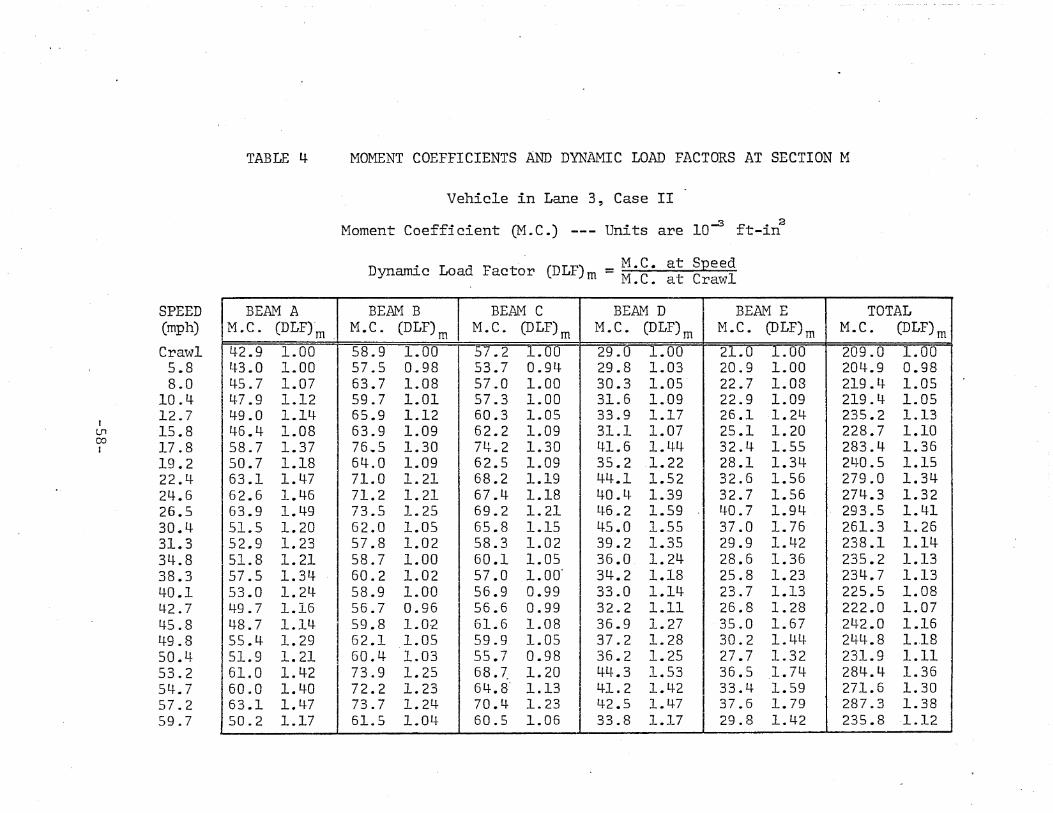
TABLE LJ. MOMENT COEFFICIENTS AND DYNAMIC LOAD FACTORS AT SECTION M
Vehicle in Lane 3, Case II
Moment Coefficient (M.C.) --- Units are lO~ ft-in2
- MaC. at SpeedDynamic Load Factor (DLF)m = M.C. at Crawl
IlJ1coI
SPEED(mph)
Crawl5.88.0
10.412.715.817.819.222.424.626.530.431.334.838.340.142.745.849.850.453.254.757.259.7
BEAM A BEAM B BEAM C BEAM D BEAM E TOTALM.C. (DLF)-m, M.C. (DLF) M.C. (DLF)m M.C. (DLF)m M.C. (DLF)m M.C. (DLF)mm
42.9 1.00 58.9 1.00 57.2 1.00 29.0 1.00 21.0 1.00 209.0 1.0043.0 1.00 57.5 0.98 53.7 0.94 29.8 1.03 20.9 1.00 204.9 0.9845.7 1.07 63.7 1.08 57.0 1.00 30.3 1.05 22.7 1.08 219.4- 1.0547.9 1.12 59.7 1.01 57.3 1.00 31.6 1.09 22.9 1.09 219.4 1.0549.0 1.14 65.9 1.12 60.3 1.05 33.9 1.17 26.1 1.24- 235.2 1.1346.4- 1.08 63.9 1.09 62.2 1.09 31.1 1.07 25.1 1.20 228.7 1.1058.7 1.37 76 .. 5 1.30 74-.2 1.30 41.6 1.44- 32.4 1.55 283.4- 1.3650.7 1.18 64-. a 1.09 62.5 1.09 35.2 1.22 28.1 1.34- 240.5 1.1563.1 1.4-7 71.0 1.21 68.2 1.19 44.1 1.52 32.6 1.56 279.0 1.3462.6 1.46 71.2 1.21 67.4 1.18 40.4- 1.-39 32.7 1.56 274.3 1.3263.9 1.4-9 73.5 1.25 69.2 1.21 46.2 1.59 40.7 1.94 293.5 1.4151.5 1.20 62.0 1.05 65.8 1.15 45.0 1.55 37.0 1.76 261.3 1.2652.9 1.23 57.8 1.02 58.3 1.02 39.2 1.35 29.9 1.42 238.1 1.14-51.8 1.21 58.7 1.00 60.1 1.05 36.0 1.24 28.6 1.36 235.2 1.1357.5 1.34- 60.2 1.02 57.0 1.00· 34-.2 1.18 25.8 1.23 234.7 1.1353.0 1.24- 58.9 1.00 56.9 0.99
I33.0 1.14 23.7 1.13 225.5 1.08
49. 7 1.16 56.7 0.96 56.6 0.99 32.2 1.11 26.8 1.28 222.0 1.0748.7 1.14- 59.8 1.0·2 61.6 1.08 36.9 1.27 35.0 1.67 242.0 1.1655.4 1.29 62.1 1.05 59.9 1.05 37.2 1.28 30.2 1.44- 21+4.8 1.,1851.9 1.21 60.4- 1.03 55.7 0.98 36.2 1.25 27.7 1.32 231.9 1.1161.0 1.42 73.9 1.25 68.7. 1.20 44.3 1.53 36.5 1.74- 284.4 1.3660.0 1.40 72.2 1.23 64.8: 1.13 41.2 1.42 33.4 1.59 271.6 1.3063.1 1.47 73.7 1.24 70.4- 1.23 42.5 1.47 37.6 1.79 287.3 1.3850.2 1.17 61.5 1.04 60.5 1.06 33.8 1.l7 29.8 1.42 235.8 -1.12
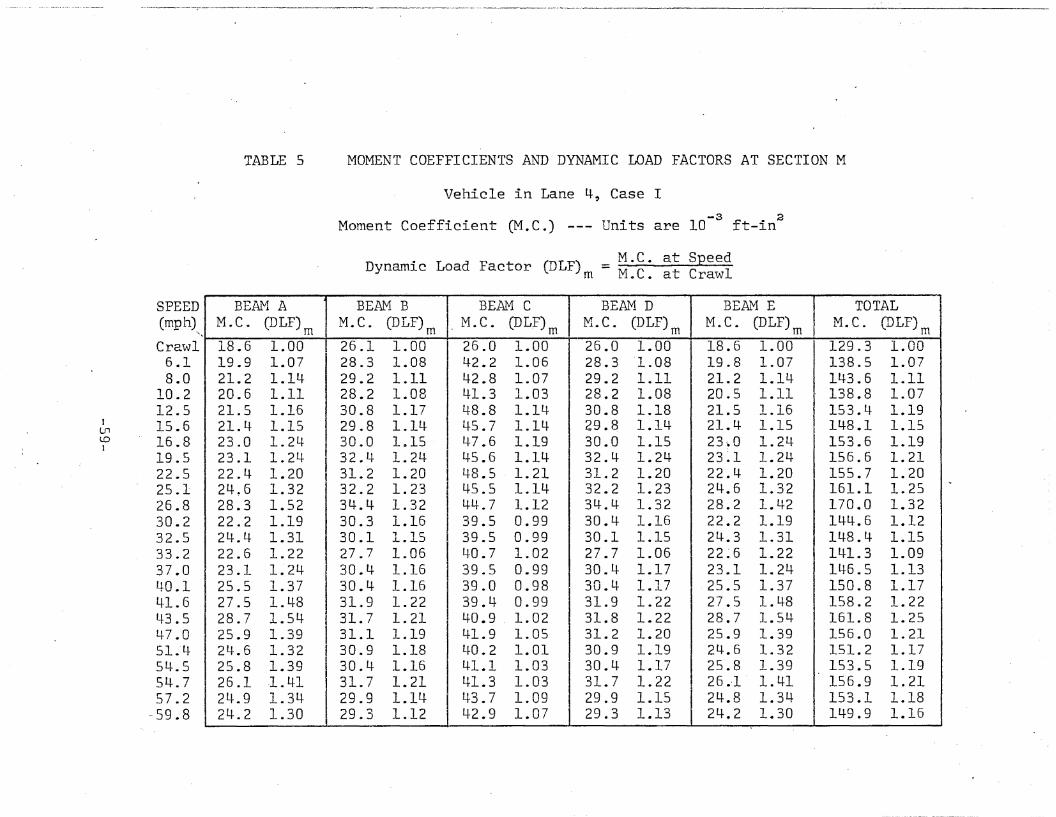
TABLE 5 MOMENT COEFFICIENTS AND DYNAMIC LOAD FACTORS AT SECTION M
Vehicle in Lane 4, Case I
Moment Coefficient (M.C.) --- Units are 10-3
ft-in2
M.C. at SpeedDynamic Load Factor (DLF)m = M.C. at Crawl
IUlto1
SPEED(mph)..
Crawl6.18.0
10.212.515.616.819.522.525.126.830.232.533.237.040.141.643.547.051.454-.55lJ..757.2
-59.8
BEAM A BEAM B BEAM C BEAM D BEAM E TOTALM.C. (DLF) M.C. (DLF) M. C. (DL,F)m M. C. (DLF) M. C. (DLF) M. C. (DLF)
m m m m m18.6 1.00 26.1 1.00 26.0 1.00 26.0 1.00 18.6 1.00 129.3 1.0019.9 1.07 28.3 1.08 42.2 1.06 28.3 '1.08 19.8 1.07 . 138.5 1.0721.2 1.14- 29.2 1.11 42.8 1.07 29.2 1.11 21.2 1.14 143.6 1.1120.6 1.11 28.2 1.08 41.3 1.03 28.2 1.08 20.5 1.11 . 138.8 1.0721.5 1.16 30.8 1.17 48.8 1.14 30.8 1.18 21.5 1.16 153.4 1.1921.4 1.15 29.8 1.14 45.7 1.14 29.8 1.14 21.4 1.15 148.1 1.1523.0 1.24 30.0 1,,15 47.6 1.19 30.0 1.15 23,~ 0 1.24 153.6 1.1923.1 1.24 32.4 1.24 45.6 1.14 32.4 1.24 23~1 1.24 156.6 1.2122.4 1.20 31.2 1.20 48.5 1.21 31.2 1.20 22.4- 1.20 155.7 1.2024~6 1.32 32.2 1.23 45.5 1.14- 32.2 1.23 24.6 1.32 161.1 1.2528.3 1.52 34.4 1.32 44.7 1.12 34.4 1.32 28.2 1.42 170.0 1.3222.2 1.19 30.3 1.16 39.5 0.99 30.4- 1.16 22.2 1.19 14-4.6 1.1224.4- 1.31 30.1 1.15 39.5 0.99 30.1 1.15 24.3 1.31 14-8.4- 1.1522.6 1.22 27.7 1.06 40.7 1.02 27.7 1.06 22~6 1.22 141.3 1.0923.1 1.24- 30.4- 1.16 39.5 0.99 30.4- 1.17 23.1 1.24- 146.5 1.1325.5 1.37 30.4- 1.16 I 39.0 0.98 30.4- 1.17 25.5 1.37 150.8 1.1727.5 1.48 31.9 1.22 39.4 0.99 31.9 1.22 27.5 1.48 158.2 1.2228.7 1.54 31.7 1.21 I 40.9 1.02 31.8 1.22 28.7 1.54 161.8 1.2525.9 1.39 31.1 1.19 41.9 1.05 31.2 1.20 25.9 1.39 156.0 1.2124.6 1.32 30.9 1.18 40.2 1.01 30.9 1.19 24.6 1.32 151.2 1.1725.8 1.39 30.4 1.16 41.1 1.03 30.4- 1.17 25.8 1.39 153.5 1.1926.1 ~1. 41 31.7 1.21 41.3 1.03 31.7 1.22 26.-1 1.41 156.9 1.2124.9 1.34 29.9 1.14- 43.7 1.09 29.9 1.15 24.8 1.34 153.1 1.1824.2 1.30 29.3 1.12 42.9 1.07 29.3 1.13 24.2 1.30 149.9 1.16
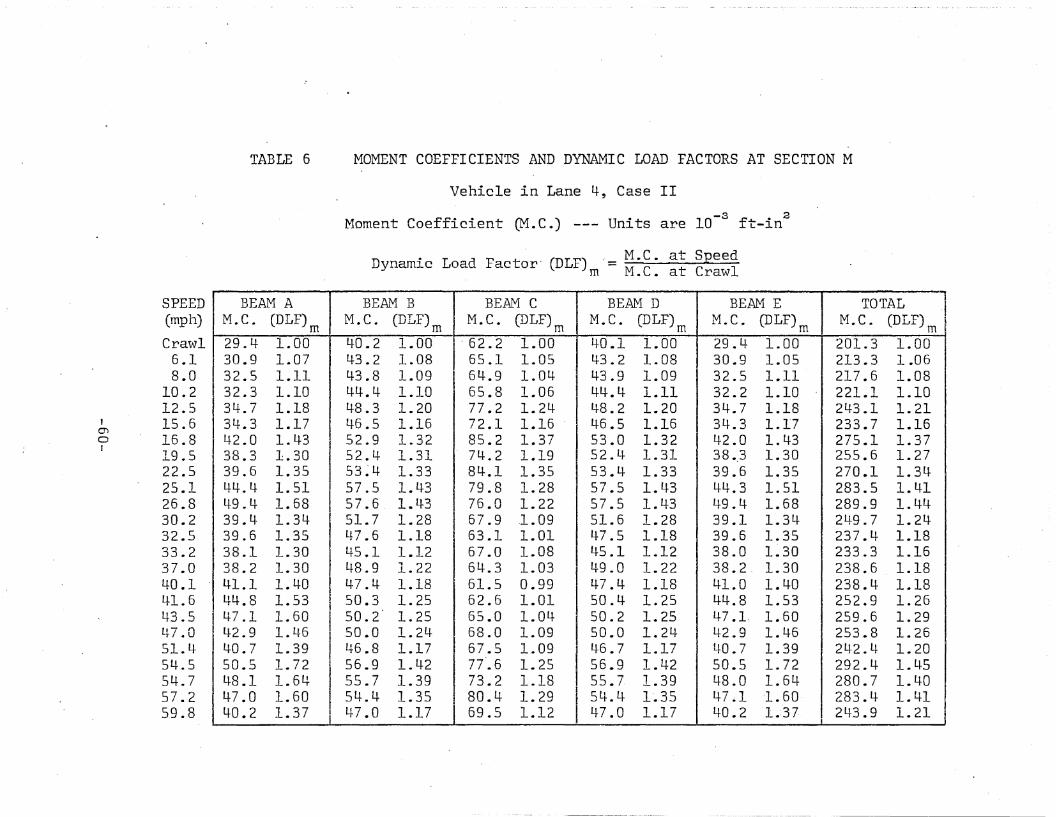
TABLE 6 MOMENT COEFFICIENTS AND DYNAMIC LOAD FACTORS AT SECTION M
Vehicle in Lane 4, Case II
Moment Coefficient (M.C.) --- Units are 10-3
ft-in2
. . M.C. at SpeedDynamic Load Factor' (DLF)m'= M.C. at Crawl
,enoI
SPEED(mph)
Crawl6.18.0
10.212.515.616.819.522.525.126.830.232.533.237.040.141.643.547.051.454.554-.757.259.8
BEAM A BEAM B BEAM C BEAtl\1 D BEAM E TOTALM. C. (DLF) M.C. (DLF) M.C. (DLF) M.C. (DLF) M.C. (DLF) M.C. (DLF)
m m m m m m29.4 1.00 40.2 1.00 ·62.2 1.00 40.1 1.00 29.4 1.00 201.3 1.0030.9 1.07 43.2 1.08 65.1 1.05 43.2 1.08 30.9 1.05 213.3 1.0632.5 1.11 43.8 1.09 64.9 1.04 43.9 1.09 32.5 1.11 217.6 1.0832.3 1.10 44.4 1.10 65.8 1.06 44.4 1.11 32.2 1.10 221.1 1.1034.7 1.18 48.3 1.20 77.2 1.24- 48.2 1.20 34.7 1.18 243.1 1.2134.3 1.17 46.5 1.16 72.1 1.16 46.5 1.16 34.3 1.17 233.7 1.1642.0 1.43 52.9 1.32 85.2 1.37 53.0 1.32 42.0 1.43 275.1 1.3738.3 1.30 52.4 1.31 74.2 1.19 52.4 1.31 38.,3 1.30 255.6 1.2739.6 1.35 53~4 1 .. 33 84.1 1.35 53.4 1.33 39.6 1.35 270.1 1.3444.4- 1.51 57.5 1.4-3 79.8 1.28 57.5 1.43 44.3 1.51 283.5 1.4149.4- 1.68 57.6 1.4-3 76.0 1.22 57.5 1.43 49.4 1.68 289.9 1.44-39.4- 1.34 51.7 1.28 67.9 -1.09 51.6 1.28 39.1 1.34- 249.7 1.24-39.6 1.35 47.6 1.18 63.1 1.01 47.5 1.18 39.6 1.35 237.4- 1.1838.1 1.30 45.1 1.12 67.0 1.08 45.1 1.12 38.0 1.30 233.3 1.1638.2 1.30 48.9 1.22 64.3 1.03 49.0 1.22 38.2 1.30 238.6 1.1841.1 1.40 47.4 1.18 61.5 0.99 47.4- 1.18 41.0 1.40 238.4 1.1844.8 1.53 50.3 1.25 62.6 1.01 50.4- 1.25 44.8 1.53 252.9 1.26
! 47.1 1.60 50.2 1.25 65.0 1.04 50.2 1.25 47 .1. 1.60 259.6 1.29j 42.9 1.46 50.0 1.24- 68.0 1.09 50.0 1.24 42.9 1.46 253.8 1.26
40.7 1.39 46.8 1.17 67.5 1.09 46.7 1.17 40.7 1.39 242.4- 1.2050.5 1.72 56.9 1.42 77>.6 1.25 56.9 1.42 50.5 1.72 292.4- 1.4548.1 1.64 55.7 1.39 73.2 1.18 S5.7- 1.39 48.0 1.64- 280.7 1.4-047.0 1.60 54.4- 1.35 80.4 1.29 54.4 1-.35 47.1 -1.60 283.4 1.4140.2 1.37 47.0 1.17 69.5 1.12 47.0 1.17 40.2 1."-37 243.9 1.21
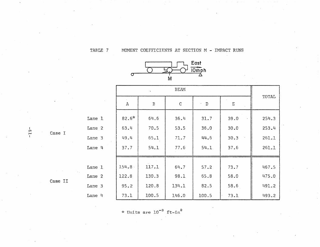
1enI-JI
Case I
Case II
T.ABLE 7
Lane 1
Lane 2
Lane 3
Lane 4
Lane 1
Lane 2
Lane 3
Lane 4
MOMENT COEFFICIENTS AT SECTION M - IMPACT RUNS
; ~Easto ~~ph
o ~
M
BEAM ITOTAL i
A B C . D E
82.6* 64.6 36.4 31.7 39.0 . I 254.3
63.4 70.5 53.5 36.0 30.0· 253.4
I 49.4- 65.1 71.7 44.6 30.3 261.1
I 37.7 54.1 77.6 54.1 37.6 261.1
154.8-- 117.1 64.7 57.2 73.7II
467.5
122.8 130.3 98.1 65.8 58.0 475.0
95.2 120.8 134.1 82.5 58.6 491.2
73.1 100.5 14-6~O 100.5 73.1 493.2
* Units are 10-3
ft-in2
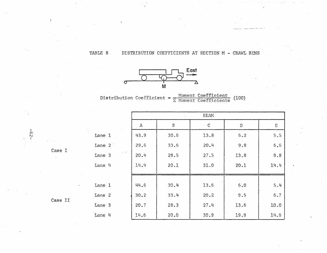
TABLE 8
.r
DISTRIBUTION COEFFICIENTS AT SECTION M - CRAWL RUNS
; lG5=Cb_~oo IM D.
Moment CoefficientDistribution Coefficient = ~ Moment Coefficients (100)
r
Lane 1O'JN
Lane 2
t
C~se ILane 3
Lane 4
Case II
Lane 1
Lane 2
Lane 3
Lane 1+
BEAM
A B C D E
43.9 30.6 13.8 6.2 5.5
29.6 33.6 20.4- 9.8 6.6
20.4 28.5 27.5 13.8 9.8
14.4 20.1 31.0 20.1 14.4-
44.6 30.4 13.6 6.0 5.4
30.2 33.4- 20.2 9.5 6.7
20.7 28.3 27.4 13.6 10.0
14.6 20.0 30.9 19.9 14.6
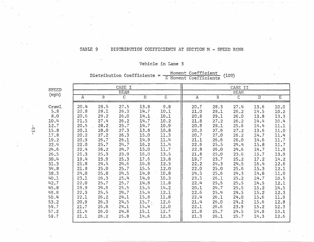
TABLE 9 'DISTRIBUTION COEFFICIENTS AT SECTION M - SPEED RUNS
Vehicle in Lane 3
Moment CoefficientDistribution Coefficients = ~ Moment Coefficients (100)
f01WJ
SPEED(mph)
Crawl5.88.0
10.412.715.817.819.222.424-.626.530.431.334.838.340.1L~2. 745.849.850.453.254.757.259.7
CASE I CASE IIBEAM BEAM
A B C D E A B C D E
20.4- 28.5 27.5 13.8 9.8 20.7 28.3 27.4 13.6 10.020.8 28.1 26.3 14-.7 10.1 21.0 28.1 26.2 14.5 10.220.6 29.2 26.0 14-.1 10.1 20.8 29.1 26.0 13.8 13.321.5 27.4- 26.2 14.7 10.2
I21.8 27.2 26.2 14..4- 10.4-
20.5 28.2 25.7 14.7 10.9 20.8 28.1 25.6 14.4- 11.1 I20.1 28.0 27.3 13.8 10.8 20.3 27.9 27.2 13.6 11.020.2 27.2 26.3 15.0 11.3 20.7 27.0 26.2 14-. -7 11.4-20.9 26.7' 26.1 14-.9 11.4- 21.1 ,26.6 26.0 14.6 11.722.0 25.7 24.7 16.2 11.4- 22.6 25.5 24.4 15.8 11.722.4- 26.2 24.7 15.0 11.7 22.8 26.0 24-.6 14.7 11.921.3 25.3 23.9 16.0 13.5 21.8 ' 25.0 23.6 15.7 13.919.4- 23.9 25.3 17.6 13.8 19.7 23.7 25.2 17.2 14-.221.8 24.5 24-.6 16.8 12.3 22.2 24.3 24.5 16.4- 12.621.8 25.0 25.7 15.5 12.0 22.0 25.0 25.6 15.3 12~124.0 25.8 24.5 14.9 . 10.8 24.5 25.6 24.3 14.6 11.023.1 26.3 25.4 14-.9 10.3 23.5 26.1 25.2 14.7 10.522.0 25.7 25.7 14.8 11.8 I 22.4- 25.5 25.5 lIt.S 12.119.9 2l+.9 25.5 15.5 14.2 20.1 24.7 25.5 15.2 14.522.3 25.5 24-. 7 15.4- 12.1 22.6 25.4 24.5 15.2 12.322.1 26.2 24.1 15.8 11.8 22.4 26.1 24-.0 15.6 11.920.9 26.3 24.5 15.7·, 12.6 21.4- 26.0 24.2' 15.6 12.821.7 26.8 24.1 ' 15.4 . 12.0 22.1 26.6 23.9 15.2 12.321.4- 26.0 24.8 15.-1 12.7 . 21.9 25,.7 24.5 14.8 13.121.1 26.2 25.8 14.6 12.3
I21.3 26.1 25.7 14.3 12.6
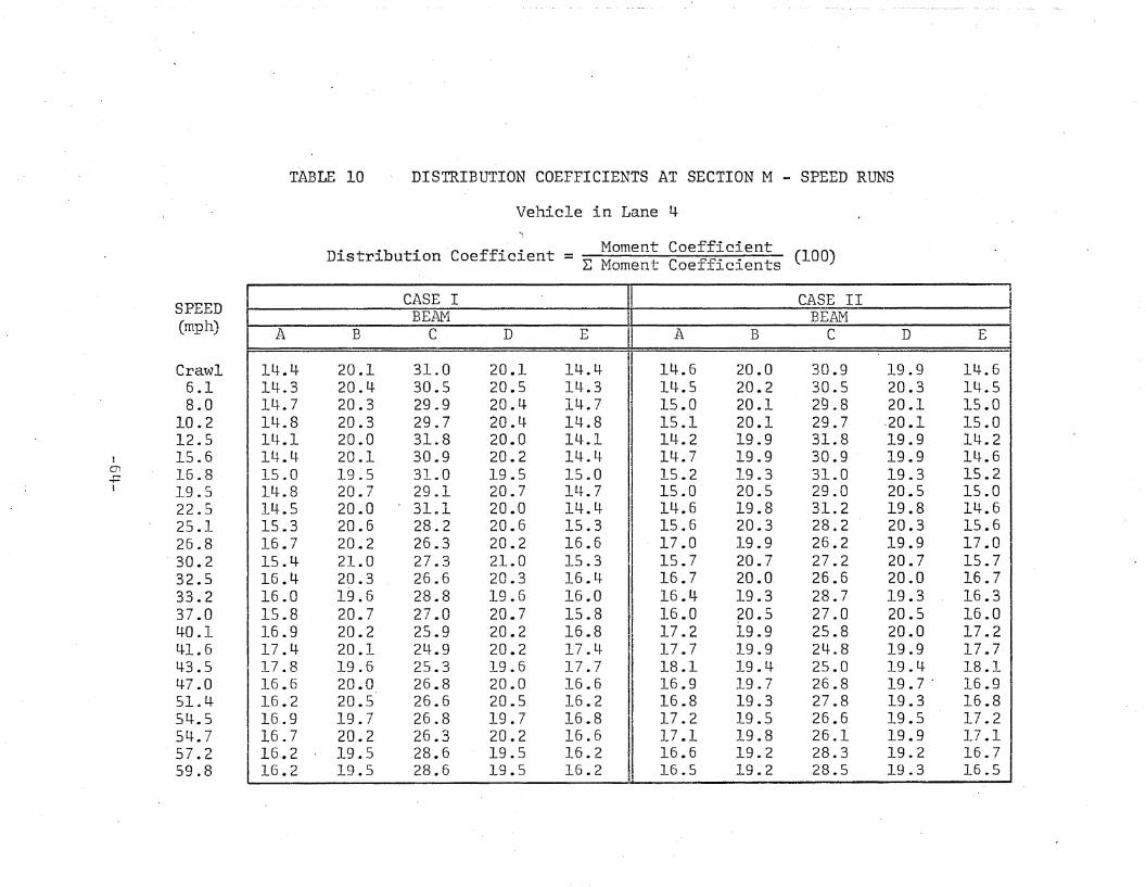
TABLE 10 DISTRIBUTION COEFFICIENTS AT SECTION M - SPEED RUNS
Vehicle in Lane 4-
IO"l+=I
SPEED(mph)
Crawl6.18.0
10.212.515.616.819.522.525.126.8
, 30.232.533.237.040.141.643.547.051.454-.554.757.259.8
. .: Moment Coefficient (100)Distribution Coefflclent = r-t 7,,roment Coefficients
CASE I CASE II iBEAM BEAM i
A B C D E A B C D E
14-.4 20.1 31.0 20.1 14.4
I
14.6 20.0 30.9 19.9 14.614.3 20.4- 30.5 20.5 14.3 14.5 20.2 30.5 20.3 14.514.7 20.3 29.9 20.4- 14.7 15.0 20.1 29.8 20.1 15.014.8 20.3 29.7 20.4- 14.8 15.1 20.1 29.7 ·20.1 15.014.1 20.0 31.8 20.0 14.1 14.2 19.9 31.8 19.9 14.214.4 20.1 30.9 20.2 14.4- 14.7 19.9 30.9 19.9 14.615.0 19.5 31.0 19.5 15.0 15.2 19.3 31.0 19.3 15.214.8 20.7 29.1 20.7 14.7 15.0 20.5 29.0 20.5 15.014.5 20.0 . 31el 20.0 14.4 14.6 19.8 31.2 19.8 14.615.3 20.6 28.2 20.6 15.3 15.6 20.3 28.2 20.3 15.616.7 20.2 26.3 20.2 16.6 17.0 19.9 26.2 19.9 17.015.4 21.0 27.3 21.0 15.3 15.7 20.7 27.2 20.7 15.716.4 20.3 26.6 20.3 16.4- 16.7 20.0 26.6 20.0 16.716.0 19.6 28.8 19.6 16.0 16.4- 19.3 28.7 19.3 16.315.8 20.7 27.0 20.7 15.8 16.0 20.5 27.0 20.5 16.016.9 20.2 25.9 20.2 16.8 17.2 19.9 25.8 20.0 17.217.4 20.1 24.9 20.2 17.4 17.7 19.9 24.8 19.9 17.717.8 19.6 25.3 19.6 17.7 18.1 19.4 25.0 19.4 18.116.6 20.0 26.8 20.0 16.6 16.9 19.7 26.8 19.7' 16.916.2 20.5 26.6 20.5 16.2 16.8 19.3 27.8 19.3 16.816.9 19.7 26.8 19.7 16.8 17.2 19.5 26.6 19.5 17.216.7 20.2 26.3 20.2 16.6 17.1 19.8 26.1 19.9 17.116.2 19.5 28.6 19.5 16.2 16.6 19.2 28.3 19.2 16.716.2 19.5 28.6 19.5 16.2 16.5 19.2 28.5 19.3 16.5
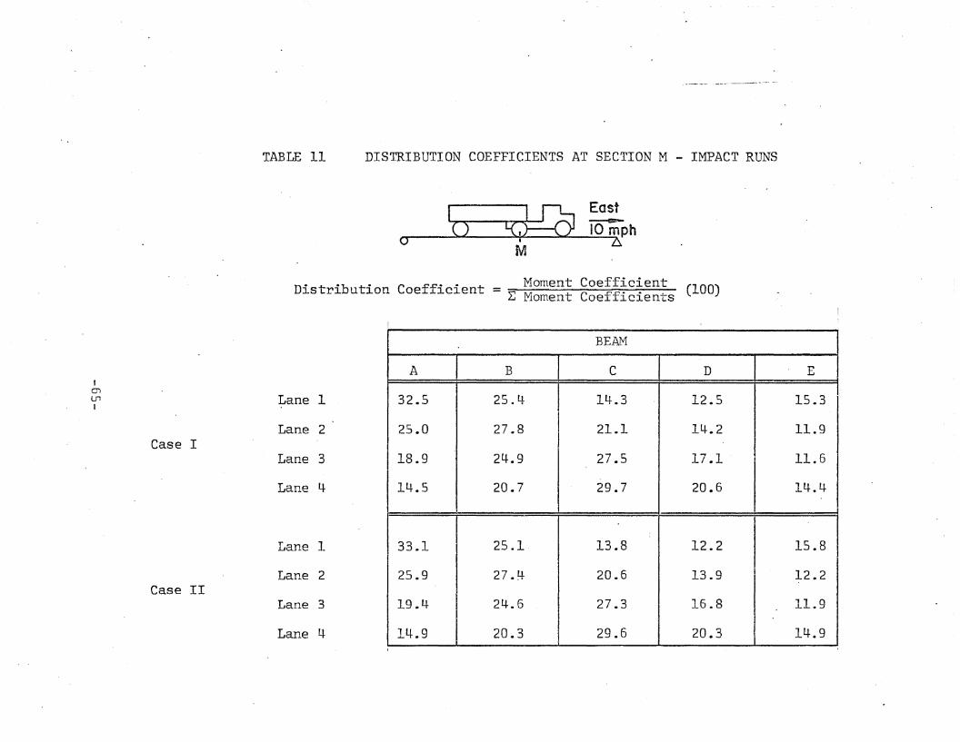
TABLE 11 DISTRIBUTION COEFFICIENTS AT SECTION M - IMPACT RUNS
o
· " .. _ Moment Coeff~c~ent (100)Dlstrlbut~on CoefflClent - ~ Moment CoefflClents
Case II
Lane 1
Lane 2
Lane 3
Lane 4-
BEAM
A B C D E
32.5 25.4- 14.3 12.5 15.3
25.0 27.8 21.1 14.2 11.9
18.9 24.9 27.5 17.1 11.6
14.5 20.7 29.7 20.6 14.4-
33.1 25.1 13.8 12.2 15.8
25.9 27.4- 20.6 13.9 12.2
19.4- 24-.6 27.3 16.8 11.9
14.9 20.3 29.6 20.3 14.9
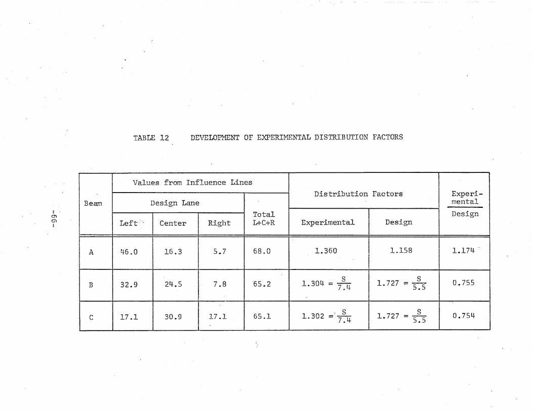
TABLE 12 DEVELOPMENT OF EXPERIMENTAL DISTRIBUTION FACTORS
Jd10)
R
Values from Influence Lines
Distribution Factors Experi-B,eam Design Lane mental
Total DesignLeft,"" Center Right L+C+R Experimental Design
A 46.0 16.3 5.7 68.0 1.360 1.158 1.174 ~
24.5 7.8 '65.2S S 0.755B 32.9 1.304- = 7.4 1.727 = 5.5
I
17.1 30.9 17.1 65.1'J S S 0.754-C 1.302 = 7.4- 1.727 = 5.5
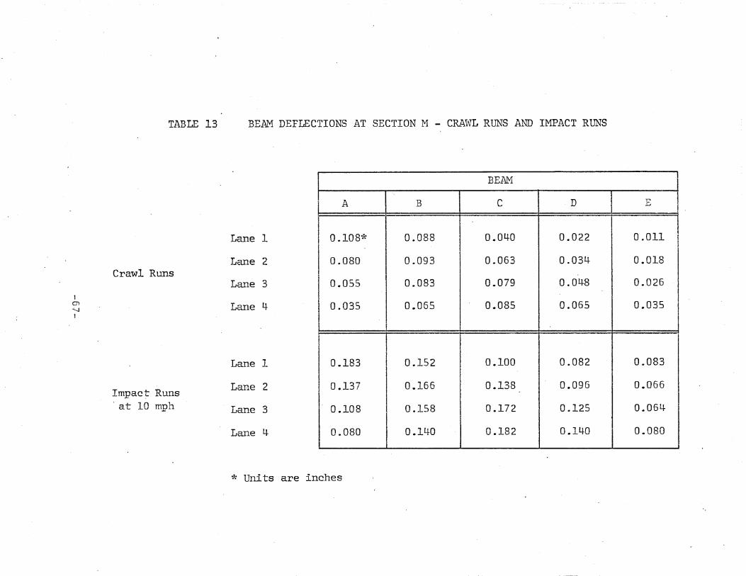
TABLE 13 BEAM DEFLECTIONS AT SECTION M - CRAWL RUNS AND IMPACT RUNS
Lane 1
Crawl RunsLane 2
1
Lane 3
Q)
"'-...Jt
Lane lJ.
Lane 1
Impac1= RunsLane 2
at 10 mph Lane 3
Lane lJ.
BEAM
A B C D rIJ...,
0.108* 0.088 0.04-0 0.022 0.011
0.080 0.093 0.063 0.034 0.018
0.055 0.083 0.079 O. 04-8 0.026
0.035 0.065 0.085 0.065 0.035
0.183 0.152 0.100 0.082 0.083
0.137 0.166 0.138 0.096 0.066
0.108 0.158 0.172 0.125 0.064
0.080 0.140 0.182 0.140 0.080
* Units are inches
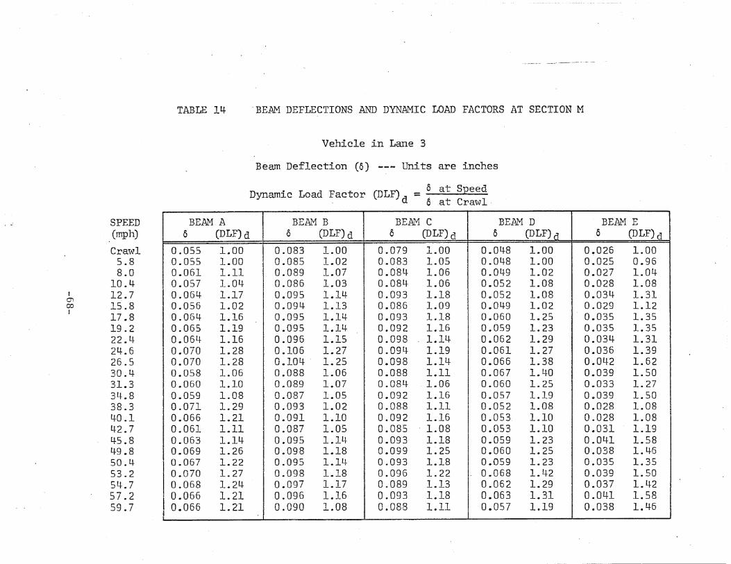
TABLE 14 "BEAM DEFLECTIONS AND DYNAMIC LOAD FACTORS AT SECTION M
Vehicle in Lane 3
Beam Deflection (0) --- Units are inches
Dynamic Load Factor (DLF) = 6 at Speedd Pi. at Crawl·
Ien00J
SPEED(mph)
Crawl5.88.0
10.412.715.817.819.222.424.626.530.431.334.838.340.142.745.849.850.453.254.. 757.259.7
BEAM A BEAM B BEAM C BEAM D BEAM E0 (DLF) d 0 (DLF) d 0 (DLF) d 0 (DLF) d 0 (DLF) d
0.055 1.00 0.083 1.00 0.079 1.00 0.048 1.00 0,026 1.000.055 1.00 0.085 1.02 0.083 1.05 0.048 1.00 0.025 0.960.061 1.11 0.089 1.07 0.084- 1.06 0.049 1.02 0.027 1.040.057 l~. 04- 0.086 1.03 0.084- 1.06 0.052 1.08 0.028 1.080.064 1.17 0.095 1.14 0.093 1.18 0 0 052 1.08 0.034- 1.310.055 1.02 0.094- 1.13 0.086 1.09 0.049 1.02 0.029 1.120.064 1.16 0.095 1.14 0.093 1.18 0.060 1.25 0.035 1.350.065 1.19 0.095 1.14- 0.092 1.16 0.059 1.23 0.035 1.350.064 1.16 0.096 1.15 0.098 . 1.14- 0.062 1.29 0.034- 1.310.070 1.28 0.106 1.27 0.094 1.19 0.061 1.27 0.036 1.390.070 1.28 0.104 . 1.25 0.098 1.14- 0.066 1.38 0.042 1.620.058 1.06 0.088 1.06 0.088 1.11 0.067 1.40 0.039 1.500.060 1.10 0.089 1.07 0.084 1.06 0.060 1.25 0.033 1.270.059 1.08 0.087 1.05 0.092 1.16 0.057 1.19 00039 1.500.071 1.29 0.093 1.02 0.088 1.11 0.052 1.08 0.028 1.080.066 1.21 0.091 1.10 0.092 1.16 0.053 1.10 0.028 1.080.061 1.11 0.087 1.05 0.085 . 1.08 0.053 1.10 0.031 1.190.063 1.14- 0.095 1.14- 0.093 1.18 0.059 1.23 0.041 1.580.069 1.26 0.098 1.18 0.099 1~2S 0.060 1.25 0.038 1.460.067 1.22 0.095 1.14- 0.093 1.18 0.059 1.23 0.035 1.350.070 1.27 0.098 1.18 0.096 1.22 . 0.068 1.42 0.039 1.500.068 1.24 0.097 1.17 0.089 1.13 0.062 1.29 0.037 1.42
I 0.066 1.21 0.096 1.16 0.093 1.18 0.063 1.31 0.041 1.58I 0.066 1.21 0.090 1.08 0.088 1.11 0.057 1.19 0.038 1.46
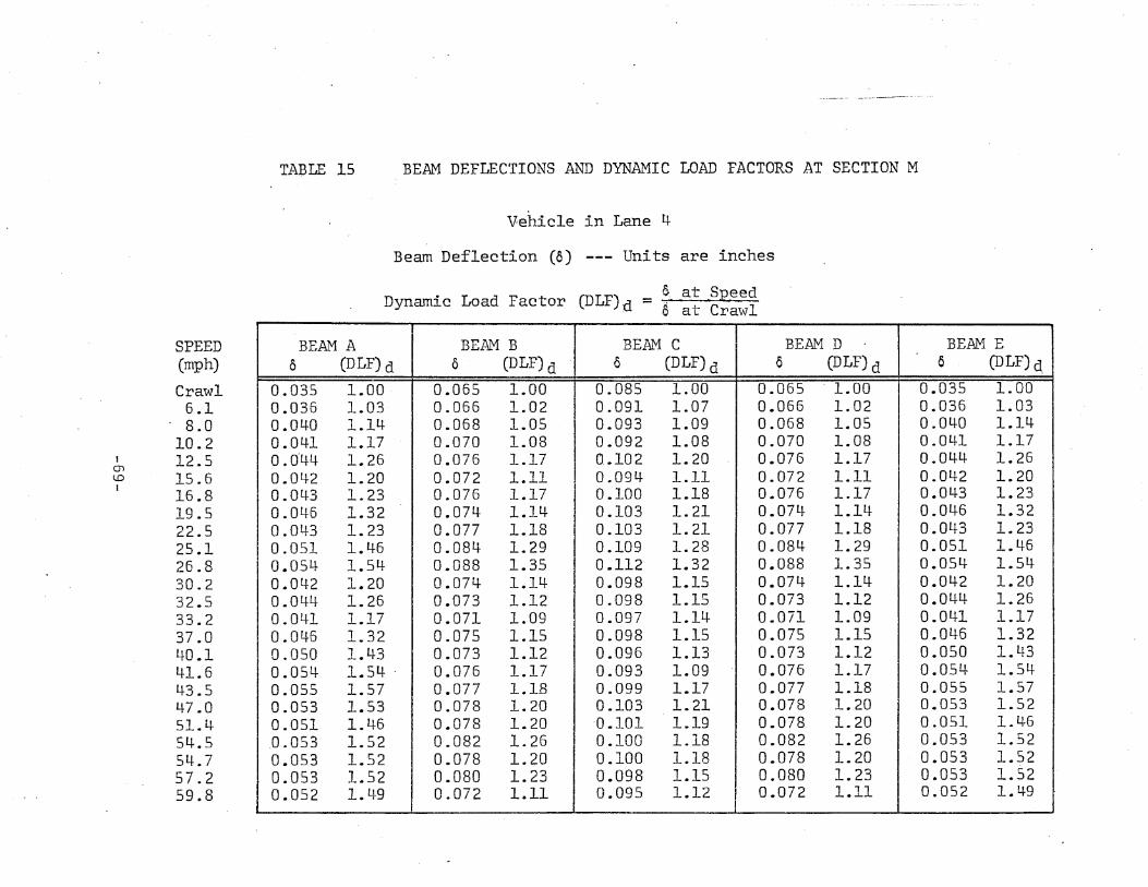
TAJ?LE 15 BEAM DEFLECTIONS AND DYNAMIC LOAD FACTORS AT SECTION M
Vehicle in Lane 4
Beam Deflection (0) --- Units are inches
Dynamic Load Factor (DLF) d = ~__at _Speed
,Q)
lDI
SPEED(mph)
Crawl6.1
. 8.010.212.515.616.819.522.525.126.830.232.533.237.040.14-1.643.547.051.454-.554..757.259.8
BEAM A BEAM B BEAM C BEAM D BEAM E0 (DLF) d 0 (DLF) d 0 (DLF) d 0 (DLF) d 0 (DLF) d,
0.035 1.00 0.065 1.00 0.085 1.00 0.065 ' 1.00 0.035 1.000.036 1.03 0.066 1.02 0.091 1.07 0.066 1.02 0.036 1.030.040 1.14- 0.068 1.05 0.093 1.09 0.068 1.05 0.040 1.14-0.041 1.17 0.070 1.08 0.092 1.08 0.070 1.08 0.041 1.170.011-4 1.26 0.076 1.17 0. .102 1.20 0.076 1.17 0.04-4- 1.260.042 1.20 0.072 1.11 0.094- 1.11 0.072 1.11 0.04-2 1.200.043 1.23 0.076 1.17 0.100 1.18 0.076 1.17 0.043 1.230.04-6 1.32 0.074 1.14 0.103 1.21 0.074 1.14- 0.04-6 1.320.043 1.23 0.077 1.18 0.103 1.21 0.077 1.18 0.043 1.230.051 1.46 0.084- 1.29 0.109 1.28 0.084 1.29 0.051 1.460.054 1.54 0.088 1.35 0.112 1.32 0.088 1.35 0.054- 1.540.042 1.20 0.074- 1.14- 0.098 1.15 0.074 1.14- 0.042 1.200.04-4 1.26 0.073 1.12 0.098 1.15 0.073 1.12 0.044- 1.260.041 1.17 0.071 1.09 0.097 1.11+ 0.071 1.09 0.041 1.170.046 1.32 0.075 1.15 0.098 1.15 0.075 1.15 0.046 1.320.050 1.43 0.073 1.12 0.096 1.13 0.073 1.12 0.050 1.430.054- 1.54 . 0.076 1.17 0.093 1.09 0.076 1.17 0.054 1.540.055 1.57 0.077 1.1B 0.099 1.17 0.077 1.18 0.055 1.570.053 1.53 0.078 1.20 0.103 1.21 0.078 1.20 0.053 1.520.051 1.46 0.078 1.20 ·0.101 1.19 0.078 1.20 0.051 1.4-6.0.053 1.52 0.082 1.26 0.100 1.18 0.082 1.26 0.053 1.520.053 1.52 0.078 1.20 0.100 1.18 0.078 1.20 0.053 1.520.053 1.52 0.080 1.23 0.098 1.15 0.080 1.23 0.053 1.520.052 1.49 0.072 1.11 0.095 1.12 0.072 1.11 0.052 1.49
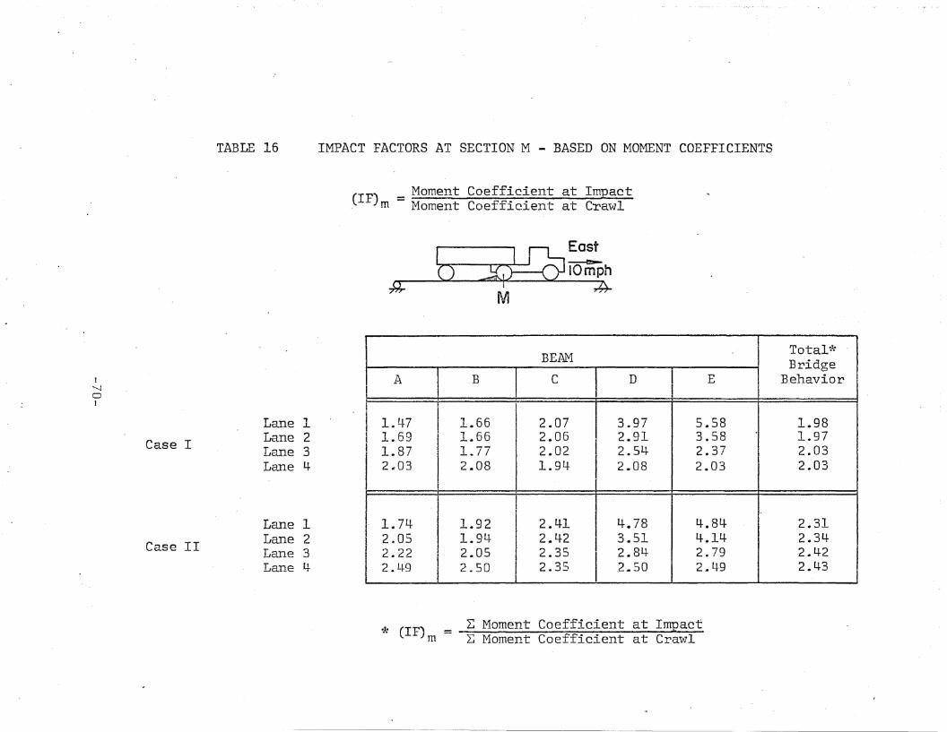
I'-JoI
Case I
Case II
TABLE 16
Lane 1Lane 2Lane 3Lane 4
Lane 1Lane 2Lane 3Lane 4
IMPACT FACTORS AT SECTION M - BASED ON MOMENT COEFFICIENTS
(IF) = Moment Coefficient at Impactm Moment Coefficient at Crawl
r~~Q~ ....~ u_ IOmph
~------- I -~
M
BEAMTotal* .Bridge
A B C D E Behavior
I II
1.47 1.66 2.07 3.97 5.58 1.981.69 1.66 2.06 2.91 3.58 1.971.87 1.77 2.02 2.54- 2.37 2.032*03 2.08 1.94- 2.08 2.03 2.03
1.74 1.92 I 2.41 4-.78 4.84 2.312.05 1.94 2.42 3.51 4.14- 2.342.22 2.05 2.35 2.84 2.79 2.4-22.49 2.50 2.35 .2.50 2 ... 49 2.43
* (IF) = L Moment Coefficient at Impactm
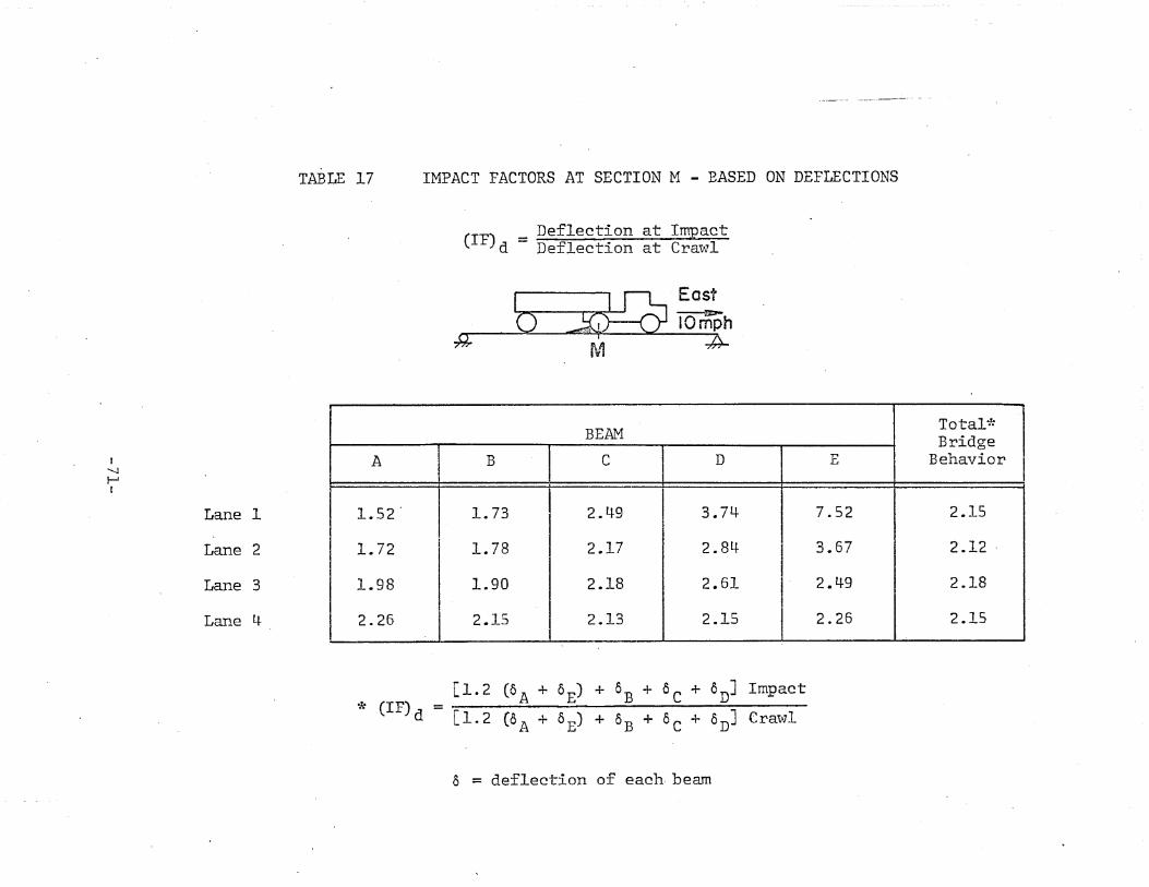
TABLE 17 IMPACT FACTORS AT SECTION M - BASED ON DEFLECTIONS
(IT)d = Deflection at Impact
*
1-........J~r
Lane 1
Lane 2
Lane 3
Lane 4-
BEAM Total*Bridge
A B C D E Behavior
1.52' 1.73 2.4-9 3.74- 7.52 2.15
1.72 I 1.78 2.17 2.84- 3.67 2.12 .
1.98 1.90 2.18 2.61 2.4-9 2.18
2.26 2.15 2.13 2.15 2.26 2.15
[1.2 (oA + 0E) + 0B + 0c + 0D] Impact* (IF)d = [1.2 (8 A + 0E) + 8B + 0c + 8D] Crawl
o = deflection of each. beam
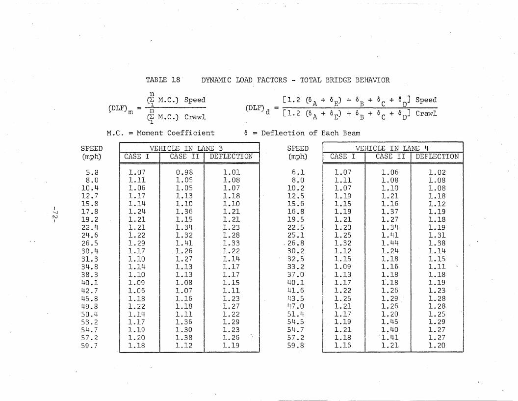
TABLE 18' DYNAMIC LOAD FACTORS - TOTAL BRIDGE BEHAVIOR
n(2: M. C.) Speed
1(DLF) = n... m
(~ M.C .)Crawl1
M.C. = Moment Coefficient
[1.2 ~A + 0E) + 0B + 0c + 0D] Speed(DLF) = -------------
d [1.2 (oA + 0E) + 0B + 0c + 0D] Crawl
o = Deflection of Each Beam
!'-Jf\.JJ
SPEED(mph)
5.88.0
10.412.715.817.819.222.424.626.530.431.334.838.340.142.745.849.850.453.254.757.259.7
VEHICLE IN LANE 3CASE I CASE II DEFLECTION
1.07 0.98 1.011.11 1.0S 1.081.06 1.05 1.071.17 1.13 1.181.14 1.10 1.101.24- 1.36 1.211.21 1.15 1.211.21 1.34- 1.231.22 1.32 1.281.29 1.41 1.331.17 .1.26 1.221.10 1.27 1.14-1.14- 1.13 1.171.10 1.13 1.171.09 1.08 1.151.06 1.07 1.111.18 1.16 1.23'1.22 1.18 1.271.14- 1.11 1.221.17 1.36 1.291.19 1.30 1.231.20 1.38 1.26 . I1.18 1.12 1.19 I
SPEED(mph)
6.18.0
10.212.515.616.819.522.525.1
.26.830.232.533.237.040.141.643.547.051.454.554.757.259.8
VEHI CLE IN LANE 4-CASE I CASE II DEFLECTION
1.07 1.06 1.021.11 1.08 1.081.07 1.10 1.081.19 1.21 1.181.15 1.16 1.121.19 1.37 1.191.21 1.27 1.181.20 1.34. 1.191.25 1.41 1.311.32 1.44- 1.381.~2 1.24 1.14-1.15 1.18 1.151.09 1.16 1.11 ..
1.13 1.18 1.181.17 1".18 1.191.22 1.26 1.231.25 1.29 1.281.21 1.26 1.281.17 1.20 1.251.19 1.45 1.291.21 1.40 1.271.18 "1.41 1.271 .. 16 1. 21~ 1.20
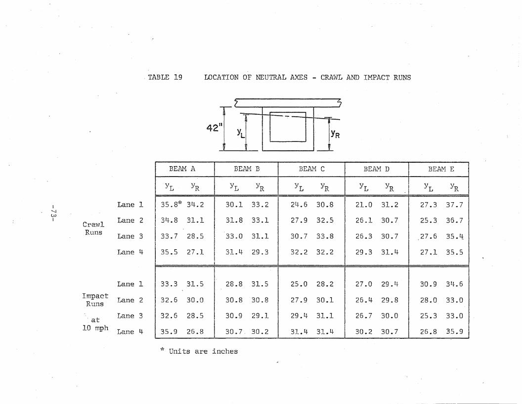
"TABLE 19 LOCATION OF NEUTRAL AXES - CRAWL AND IMPACT RUNS
42 11
YR
1 Lane 1'-JLt.Jt
Crawl Lane 2
Runs Lane 3
Lane 4-
Lane I.
Impact Lane 2Runs
Lane 3. a"t
10 mphLane 4
BEAM A BEAM B BEAM C BEAM D BEAM E
YL YR YL YR YL YR YL YR YL YR
35.8* 3I.l.2 30.1 33.2 24.6 30.8 21.0 31.2 27.3 37.7
34.8 31.1 31.8 33.1 27.9 32.5 26.1 30.7 25.3 36.7
33.7 28.5 33.0 31.1 30.7 33.8 26.3 30.7 27.6 35.4
35.5 27.1 I 31.4 29.3 32.2 32.2 29.3 31.4- 27.1 35.5
33.3 31.5 28.8 31.5 25.0 28.2 27.0 29.4 30.9 34.6
32.6 30.0 30.8 30.8 27.9 30.1 26.4- 29.8 28.0 33.0
32.6 28.5 30.9 29.1 29.4- 31.1 26.7 30.0 25.3 33.0
35.9 26.8 30.7. 30.2 31.4 31.4- 30.2 30.7 26.8 35.9
* Units are inches
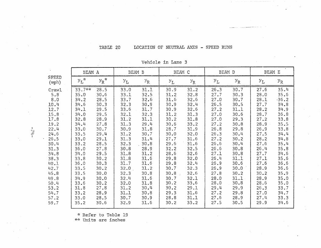
TABLE 20 LOCATION OF NEUTRAL AXES - SPEED RUNS
Vehicle in Lane 3
SPEED(mph)
Crawl5.S-8.0
10.412.715.817.819.2
~ 22.4-f 24.6
. 26.530.431.334.838.340.142.745.849.850.453.254-. 757.259.7
BEAM A BEAM B BEAM C BEAM D BEAM E
y * y * YL YR YL YR YL YR YL YRL R
33.7** 28.5 33.0 31.1 30.9 31.2 26.3 30.7 27.6 35.435;0 30.6 33.1 32.5 31.2 32.8 27.7 30.3 28.0 35.634.2 28.5 33.7 32.6 31.6 32.6 27.0 30.7 28.1 ·36.234-.6 30.3 32.3 30.9 30.9 32.4- 26.5 30.5 27.7 34.834.1 29.5 33.6 31.7 30.9 32.6 27.2 31.1 28.2 34.934.0 29.5 32.1 32.3 31.2 31.3 27.0 30.6 28.7 36.832.8 28.9 31.2 31.1 30.2 31.8 27.0 29.3 27.2 33.834-.4- 27.8 31.3 29 .4- 30.6 33.2 27.2 30.8 28.9 35.533.0 30.7 30.9 31.8 28.7 31.9 26.8 29.8 26.9 33.833.5 29.4- 31.2 30.7 30.0 32.0 26.3 30.4 27.5 34-.433.0 29.1 31.3 31.4- 27.7 31.6 27.2 30.2 28.2 34.833.2 28.5 32.3 30.8 29.6 31.6 26.6 30.4 27.6 35.436.0 27.8 30.8 28.9 32.2 32.5 26.6 30.8 26.4- 35.834.0 29.5 31.8 31.2 28.6 .32.6 27.1 3008 27.7 34.633.8 30.2 31.8 31.6 29.8 32.0 26.1+ 31.1 27.1 35 0636.0 30.3 31.7 31.6 29.8 32.4 26.9 30.6 27.6 36.633.5 30.2 32.0 31.2 30.7 32.3 26.9 30.0 28.9 36.633.5 30 .. 0 32.3 30.8 30.8 . 32.6 27.8 30.2 30.2 35.934-.9 30.0 32.4- 31.6 30.7 32.1 28.0 31.1 . 28.9 35.033.6 30.2 32.0 31.8 30.2 33.6 28.0 30.8 28.6 35.031.8 27.8 31.2 30.4 30.2 29.1 29.4 29.9 26.3 33.733.2 28.9 31.1 30.8 29.3 31.6 27.2 29.8 27.0 34-.733.0 28.5 30.7 30.9 28.8 31.1 27.6 28.9 27.4 33.335.2 30.6 32.9 31.6 30.2 33.2 27.5 30.5 29.9 34.6
* Refer to Table 19** Units are inches
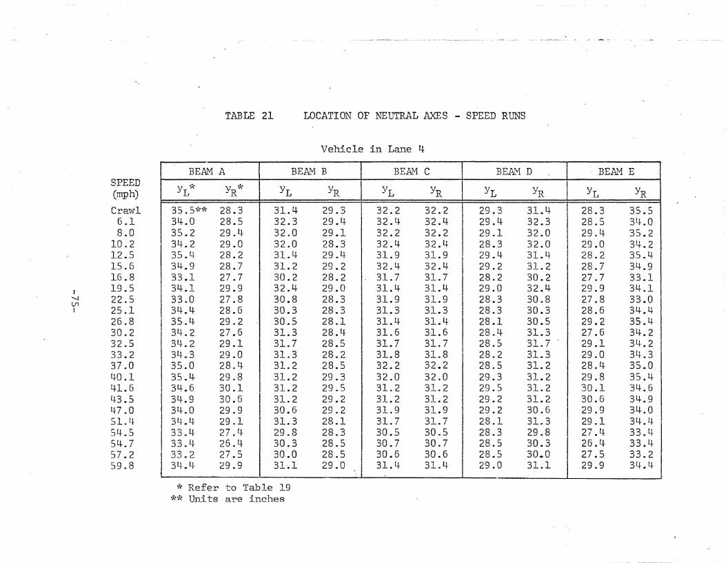
TABLE 21 LOCATION OF NEUTRAL AXES - SPEED RUNS
Vehicle in Lane 4
BEAM A BEAM B BEAL'1 C
YL YR I YL YR
. BEAM EBEAM D
29.3 31.4 I 28.3 35.529.4 32.3 28.5 34.029.1 32.0 29.4 35.228.3 32.0 29.0 34.229.4 31.4 28.2 35.429.2 31.2 28.7 34.928.2 30.2 27.7 33.129.0 32.4- 29.9 34.128.3 30.8 27.8 33.028.3 30.3 28.6 34.428.1 30.5 29.2 35.428.4 31.3 27.6 34.228.5 31.7 - 29.1 34.228.-2 31.3 29.0 34.328.5 31.2 28.4 35.029.3 31.2 29.8 35.429.5 31.2 30.1 34.629.2 31.2 30.6 34.929.2 30.6 29.9 3~.O
28.1 31.3 29.1 34.428.3 29.8 27.4 33.428.5 30.3 26.4 33.428.5 30.0 I 27.5 33.2129.0 31.1 29.9 34.4
J
YR
32.232.432.232.431.932.431.731.431.931.331.431.631.731.832.232.031.231.231.931.730 .. 530.730.631.4
YL
32.232.432.232.431.932.431.731.431.931.331.431.631.731.832.232.031.231.231.931.730.530.730.631.4
YR
29.329.429.128.329.429.228.229.028.328.328.128.428.528.228.529.329.529.229.228.128.328.528.529.0
YL
31.432.332.032.031.431.230.232.430.830.330.531.331 ..731.331.231.231.231.230.631.329.830.330.031.1
YR*
28.328.529.429.028.228.727.729.927.828.629.227.629.129.028.429.830.130.629.929.127.426.427.529.9
YL*35.5**34-.035.234.235.434.933.134.133.034.435.434.234.234.335.035.434-.634.934-.034.433.1+33.433.234.4
SPEED(mph)
Crawl6.18.0
10.212.515.616.819.522.525.126.830.232.533.237.040.141.643.547.051.454-.554.757.259.8
J'-.JLnI
* Refer to Table 19** Units are inches
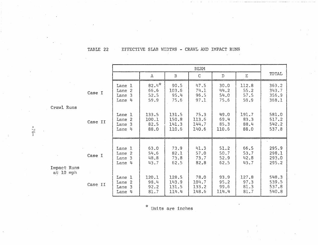
I'-J01J
Crawl Runs
Impact Runsa~ 10 mph
TABLE 22
Case I
Case II
Case I
Case II
EFFECTIVE SLAB WIDTHS - CRAWL AND IMPACT RUNS
BEAM I
A B C D E TOTAL 1
Lane 1 82.4* 90.5 47.5 30.0 112.8 363.2Lane 2 66.6 103.6 74.1 "44.2 55.2 343.7 .Lane 3 52.5 95.4- 96.5 54.0 57.5 356.9 ILane 4- 59.9 75.6 97.1 75.6 59.9 368.1
Lane 1 133.5 131.5 75.3 49.0 191.7 581.0Lane 2 100.1 150.8 113.6 69.4- 83.3 517.2Lane 3 82.5 141.3 144.7 85.3 88.4 542.2Lane 4- 88.0 110.6 140.6 110.6 88.0 537.8
Lane 1 63.0 73.9 41.3 51.2 66.5 295.9Lane 2 54.6 82.1 57.0 50.7 53.7 298.1Lane 3 48.8 73.8 73.7 52.9 42.8 293.0Lane 4- 43.7 62.5 82.8 62.5 43.7 295.2
Lane 1 120.1 128.5 78.0 93.9 127.8 54-8.3Lane 2 98.4 143.9 104-.7 95.2 97.3 539.5Lane 3 92.2 131.5 133.2 99.5 81.3 537.8Lane 4- 81.7 114.4- 148.6 114-.4- 81.7 540.8
*. hUnlts are inc es
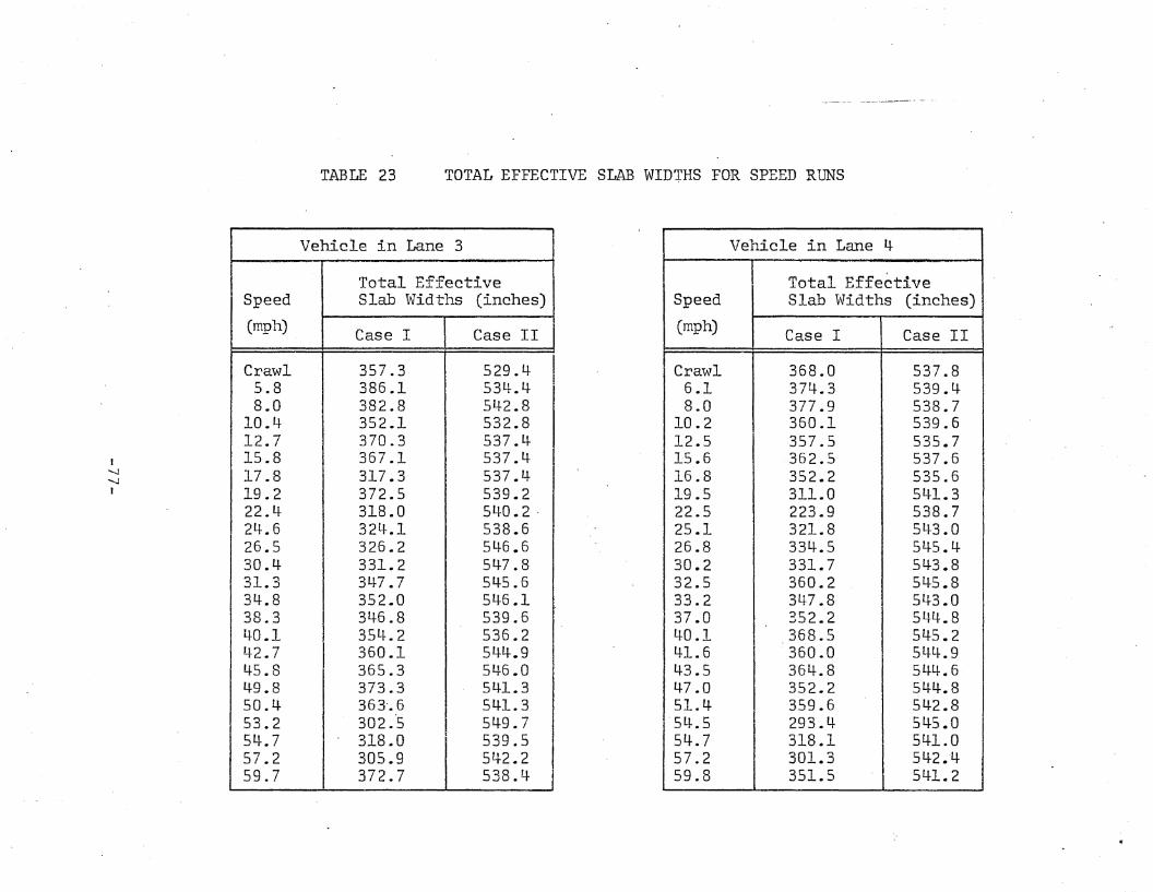
TABLE 23 TOTAL EFFECTIVE SLAB WID'rHS FOR SPEED RUNS
f-......j
'-Jf
Vehicle in Lane 3
Total EffectiveSpeed Slab Widths (inches)
(mph) Case I Case II
Crawl 357.3 529.4 I5.8 386.1 534-.4-8.0 382.8 54-2.8
10.4- 352.1 532.812.7 370.3 537.4-15.8 367.1 537.4-17.8 317.3 537.4-19.2 372.5 539.222.4- 318.0 54-0.2 .24.6 324-.1 538.626.5 326.2 546.630.4 331.2 54-7 .831.3 34-7.7 545.634-.8 352.0 51+6 .138.3 34-6.8 539.640.1 354-.2 536.242.7 360.1 544.945.8 365.3 546.04-9.8 373.3 541.350.4- 363-.6 541.353.2 302.'5 54-9.754-. 7 318.0 539.557.2 305.9 54-2. 259.7 372.7 538.4
Vehicle in Lane 4
Total E,ffectiveSpeed Slab Widths (inches)
(mph) Case I Case II
Crawl 368.0 537.85.1 374-.3 539.4-8.0 377.9 538.7
10.2 360.1 539.612.5 357.5 535.715.6 362.5 537.616.8 352.2 535.619.5 311.0 54-1.322.5 223.9 538.725.1 321.8 543.026.8 334-.5 545. 1+30.2 331.7 543.832.5 360.2 54-5.833.2 347.8 54-3.037.0 352.2 544-.840.1 368.5 54-5.241.6 360.0 544-.943.5 364.8 54-4. 647.0 352.2 544-.851.4- 359.6 542.8
·5 tJ..5 293.4- 54-5.054-. 7 318.1 54-1.057.2 301.3 54-2.-459.8 351.5 54-1.2
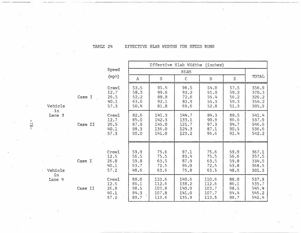
TABLE 24 EFFECTIVE SLAB WIDTHS FOR SPEED RUNS
I-.JcoJ
Vehiclein
Lane 3
Vehiclein
Lane 4-
Case I
Case II
Case I
Case II
Speed
(mph)
Crawl12.726.540.157.3
Crawl12.726.540.1
'57.3
Crawl12.5-26.840.157.2
Crawl12.526.840.157.2
Effective Slab Widths (inches)
BEAM
A B C D ETOTAL
53.5 95.4 96.5 54.0 57.5 356.958.3 99.6 92.2 61.0 59.2 370.352.2 88.8 72.6 56.4- 56.2 326.2
-63.6 92.1 82.-9 56.3 59.3 354.250.4 81.8 69.6 52.8 51.3 305.9
82.6 141.3 144.7 84.3 88.5 541.4-85.0 142.3 133.1 90.9 86.6 537.987.9 145.0 121.7 97.3 94. '7. 546.698.3 136.0 124.3 87.1 90.5 536.690.0 141.0 :J-23.2 96.6 91.4 542.- 2
59.9 75.6 97.1 75.6 59.9 367.156.5 75.5 93.4- 75.5 56.6 357.559.8 63.5 87.9 63.5 59.8 334.563.7 72.5 96.0 72.5 63.8 368.548.6 63.6 76.8 63.5 48.6 301.3
88.0 110.6 140.6 110.6 88.0 537.986.1 112.6 138.2 112.6 86.1 535.798.5 103.8 140.9 103.7 98.5 545.4-94.3 107.8 141.0 107.7 94.4- 545.289.7 113.6 135.9 113.5 89.7 542.4
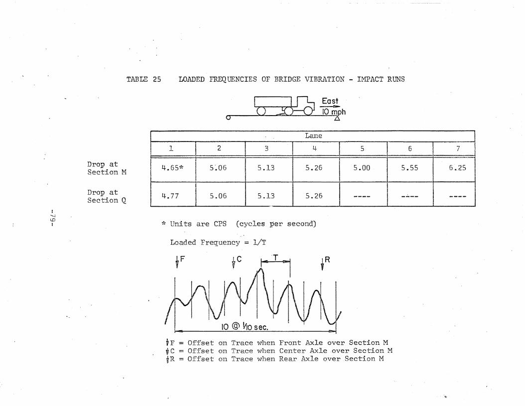
TABLE 25 LOADED FREQUENCIES OF BRIDGE VIBRATION - IMPACT RUNS
I ~ East() :x ~ha ~
1'-JtoI
Drop atSection M
Drop atSection Q
Lane
1 2 3 4 5 6 7 t~
-JI
4.65* 5~O6 5.13 5.26 5.00 5.55 6 •. 25
4-.77 5.06 5.13 5.26 --~- ---- -~--
* Units are CPS (cycles per second)
Loaded Frequency = liT
,F ,c
10 @ ~o sec.
,R
VF = Offset on Trace when Front Axle over Section MWe = Offset on Trace when Cente~ Axle .over Section MtR = Offset on Trace when Rear Axle over Section M
'..,.
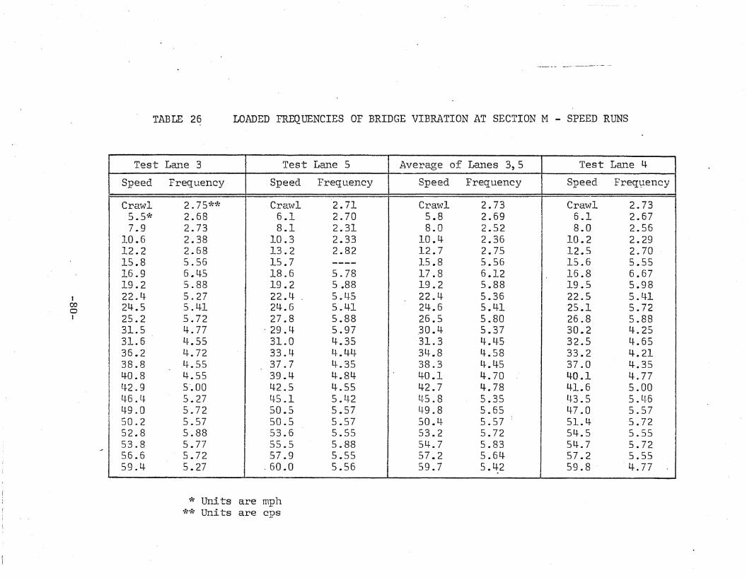
TABLE 26 LOADED FREQUENCIES OF BRIDGE VIBRATION AT SECTION M - SPEED RUNS
tcoaI
Test Lane 3 Test Lane 5 Average of Lanes 3,5 Test Lane 4-
Speed Frequency Speed Frequency Speed Frequency Speed Freq\lency
Crawl 2.75** Crawl 2.71 Crawl 2.73 Crawl 2.735.5* 2.68 6.1 2.70 5.8 2.69 6.1 2.577.9 2.73 8.1 2.31 8.0 2.52 8.0 2.56
10.6 2.38 10.3 2.33 10.4 2.36 10.2 2.2912.2 2.68 13.2 2.82 12.7 2.75 12.5 2.7015.8 5.56 15.7 ---- 15.8 5.56 15.6 5.5516.9 6.45 18.6 5.78 17.8 6.12 16.8 6.6719.2 5.88 19.2 5 .88 19.2 5.88 19.5 5.9822.4 5.27 22.4 . 5.4-5 22.4- 5.36 22.5 5.4124.5 5.41 24-.6 5.41 24.6 5.4-1 25.1 5.7225.2 5.72 27.8 5.88 26.5 5.80 26.8 5.8831.5 4.77 ' 29.4- 5.97 30.4- 5.37 30.2 4.2531.6 4.55 31.0 4.35 31.3 4-.45 32.5 4.6536.2 4-.72 33.4- 4.4-4- 34-.8 4-.58 33.2 4.2138.8 4.-55 37.7 4-.35 38.3 It.4-5 37.0 4.354-0.8 4.55 39.4- 4.84- 4-0.1 4-.70 40.1 4.77
I 42.9 5·.00 42.5 4-.55 4-2.7 4.78 4-1.6 5.00i 46.4- 5.27 45.1 5.42 45.8 5.35 43.5 5.4-6I 49.0 5.72 50.5 5.57 4-9.8 5.65 47.0 5.57I 50.2 5.57 50.5 5.57 50.4 5.57 51.4 5.72
52.8 5.88 53.6 5.55 53.2 5.72 54-.5 5.5553.8 5.77 55.5 5.88 54.7 5.83 54-.7 5.725.6.6 5.72 57.9 5.55 57.2 5.64- 57.2 5.5559.4 5.27 .60.0 5.56 59.7 5.42 59.8 . 4.77
* Units are mph** Units are cps
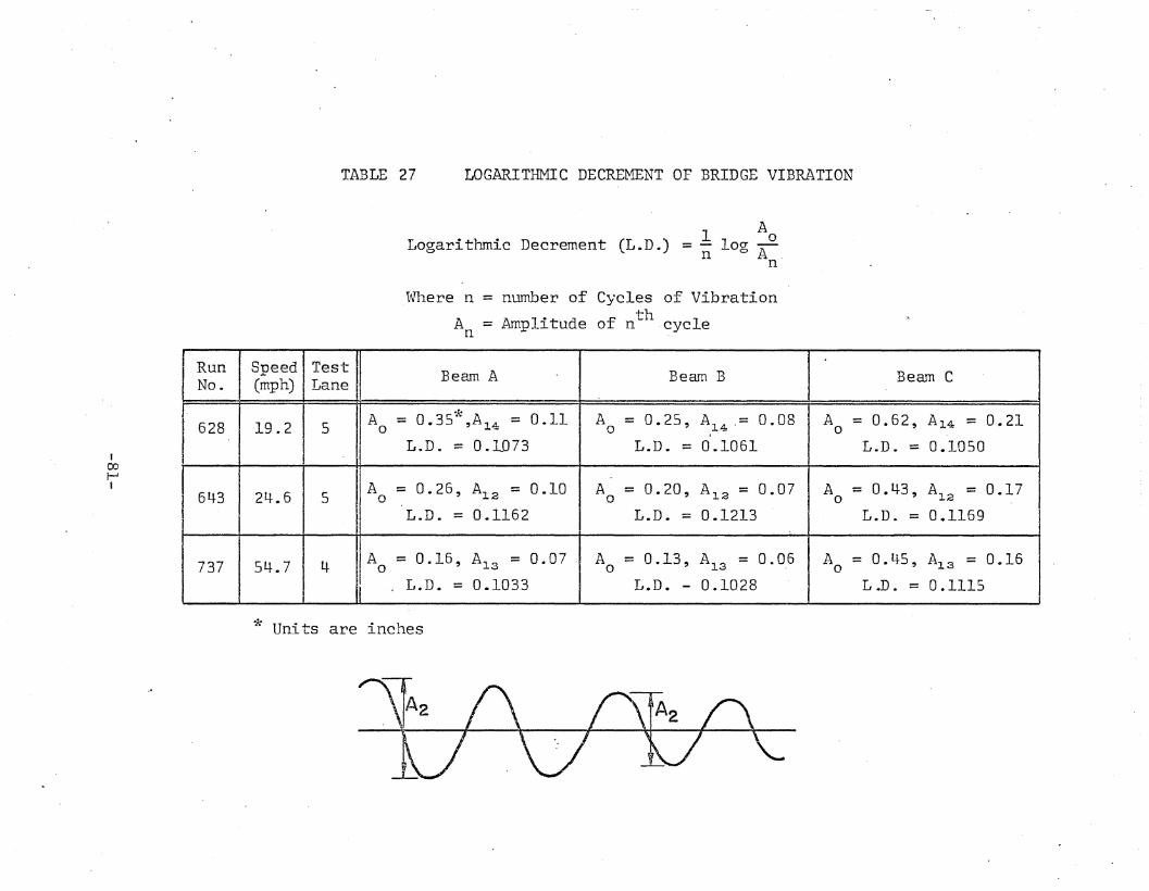
TABLE 27 LOGARITHMIC DECREMENT OF BRIDGE VIBRATION
tcol--'I
ALogarithmic Decrement (L.D.) = ~ log AO
n
Where n = number of Cycles of Vibration
A = Amplitude of nth cyclen
Run Speed Test Beam A Beam B Beam CNo. (mph) Lane
* Ao = 0.25, ~14= 0.08 A = 0.62, A14 = 0.21628 19.2 5 A = 0.35 ,Al~ = 0.11o - 0
L.D. = 0.1073 L.D. = 0.1061 L.D. = 0.1050
643 24.6 5Ao = 0.26, A12 = 0.10 Ao = 0.20, A12 = 0.07 A = 0.43, A12 = 0.17o .
L.D. = 0.1162 L.D. ::: 0.1213 L.D. = 0.1169
737 54.7 4- Ao = 0.16, A13 = 0.07 Ao = 0.13, A13 = O.~6 Ao = 0.45, A13 = 0.16
J L.D. = 0.1033 L. D. - O. 1028 L.D. = 0.1115
* Units are inches
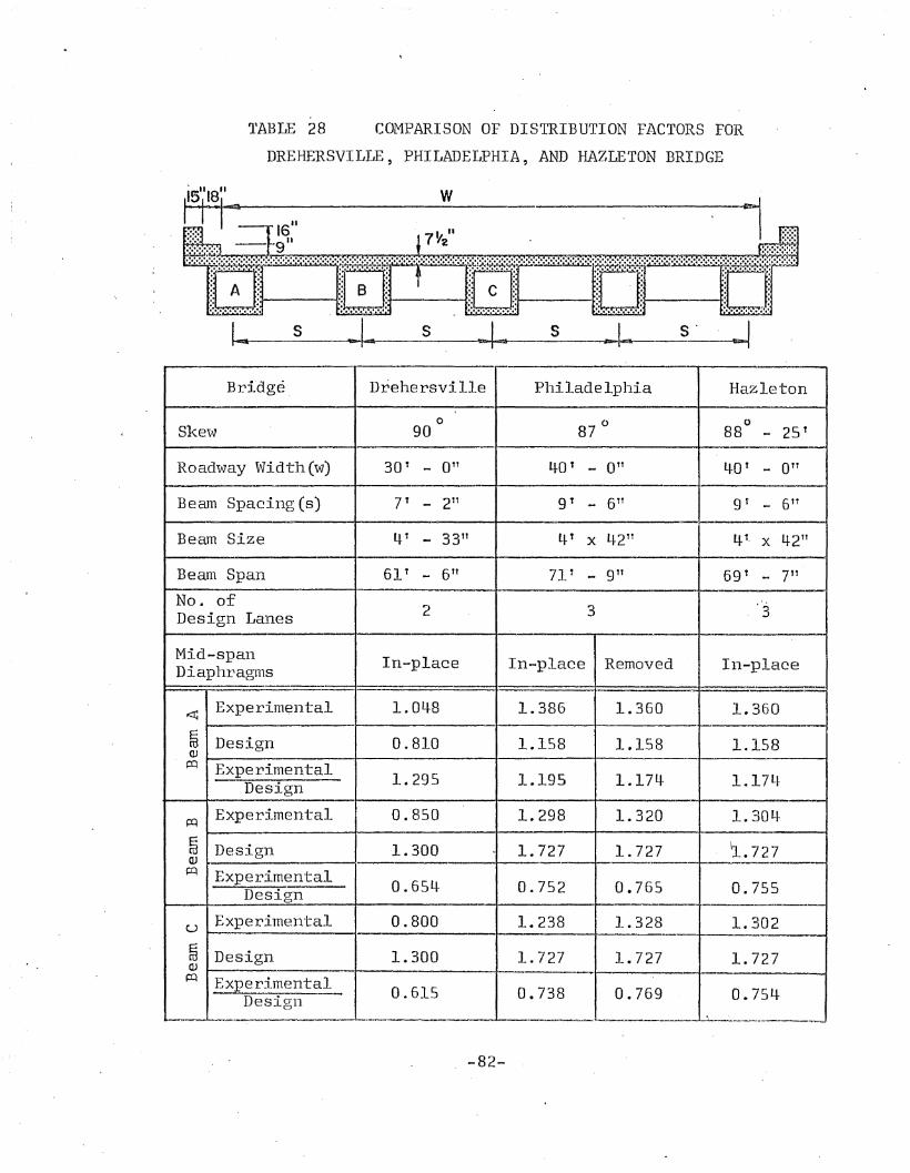
TABLE 28 COMPARISON OF DISTRIBUTION FACTORS FOR
DREHERSVILLE, PHILADELPHIA, AND HAZLETON BRIDGE
-Bridge _ Drehersville Philadelphia Hazleton
087 0
0Sl<ew 90 88 - 25'
Roadway Width (w) 3D' _ 011 ltD' _ Off 40' _ OTTA_
Beam Spacing (8) 7' - 2tt gT - 6 TT gt - 6ft
Be-am Size 4 ' - 33" 4' x 42 Tt 41. X 42 11
Beam Span 61 ' - 6Tt 71' _ gTt 69' - 7ft
No. of2 3 3Design Lanes
Mid-span In-place In-place Removed In-placeDiaphragms"~
~Experimental 1.04-8 1.386 1.360 1.360
ffi Design 0.810 1.158 1.158 1.158Q)
P=l ExperimentalDesign 1.295 1.195 1.174· 1.17 l t
~Experimental 0.850 1.298 1.320 1.304
~ Design 1.300 1.727 1.727 \1. 727QJ --
p:'.:l ExperimentalDesign 0.654- 0.752 0.765 0.755
u Experimental 0.800 1.238 1.328 1.302-~ Design 1.300 1.727 1.727 1.727OJ~ Experimental
Desig11 0.615 0.738 0.769 0.754...._. ~_....--_________ -L-.~__~~._~.____~_
-82-
-f
10. FIGURES
-83-
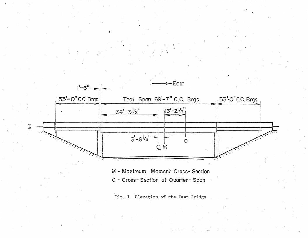
·
1~_6n- ~East
! .;!! . r3-6'/21· Q
G;.. ~J1
""'4: ~ II n:) ... -:;; ~2
, t OnC IL I 7 11 . 3 I n CC 833 .C.Brgs.j Test Span 69- C.C. Brgs. -/1..;3-0 .. rg~
100+=J
M - Maximum ~.J1oment Cross- Section
Q - Cross- Section at Quarter- Span
fig. 1 Elevation of the Test Bridge
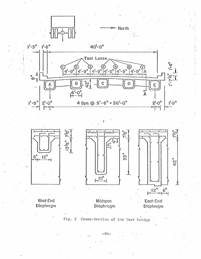
~ North
,- ..
= L. mTL-.r-...~----'T/=~
. ~'_O~
4 Spa. @ 9'- e" :: 38 1-0"
) .
A I
I2'-0"~.~
¢
-.!..~
~-[1'--, I
\'Vesf-EndDiaphragm
(I •
. MidspanDiapt1ragm
-C'J~
East ..·EnclQiaphragm
Fig. 2, .
Cross-S~ctioh of the Test Bridge.
-85-
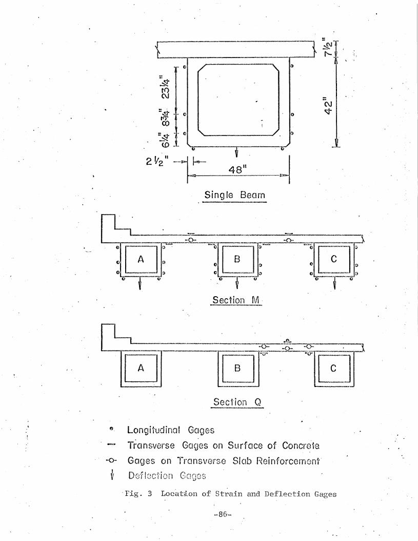
o
. 0o
--. ,-~__481l_~
Single Bearn
Sectioll Q
-0-
Longitudinal Gages
Transverse Gages on Surface of Concre1e
Gages 011 l-ransverse Slab ReirlforcE~m'orlt·
D(~f I(~ctic)rl GCJQas
, Fig. 3 Locatd.o11 of Strain and Deflection Gages
~.. 86·-
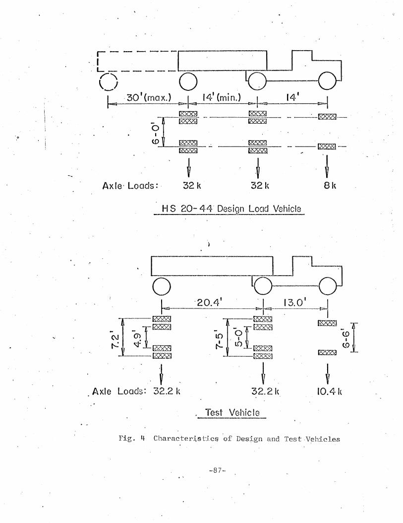
8k
--~-
'~
--'~_.
321,32 kAxle' Loads: '
· r - - - -- -[.-",L - .r," /'............
~30t(maX.)
H S 20-- 44' Desi~n Load Vehicle
", fAxle Loads: 32.2 1<
~ Test Veliic Ie
Fig. 4 Character~stica of Desfgn and Test·V~hicles
-87-
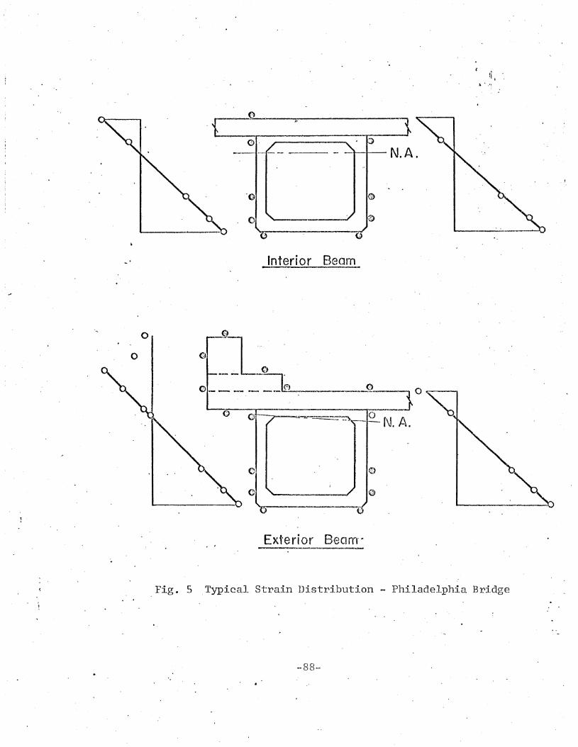
o
o
o·1--1--- N. A.
o
J[lterior 'Bearn
1':':\ 0} 0v - - -. -- -- -.-----...-=-~0
() 0 ~~_o N~A.
o~--------""""""
Exterior Beam·"
Fig. 5 .Typical Strain Distribution - Philadelphia Bridge
t.
··88-
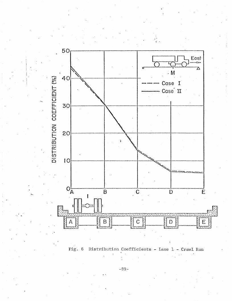
50------,..------,..-------~----,
. '0 4 OJ--~-'\!~----t------r-~, --- Case Iz ~.~ Cose~ ITwoLL 30...---~--t~--_·-"f ---LLtLJoU
z~ 201------1----'\.~:Jro~
l(f)
·0 IOt-------t--------t--~~--+-----
Fig. 6 Distribution Coefficients - Lane 1 - Crawl Run
-89~
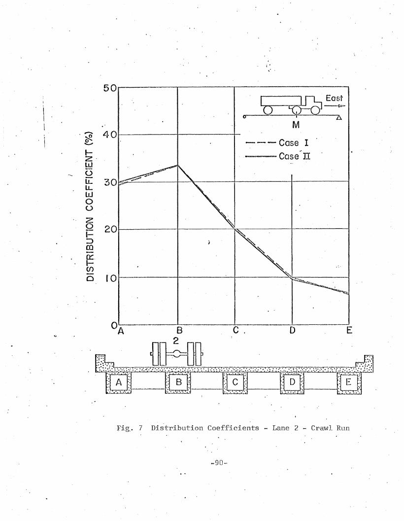
50-----~----~-----------,
o
401--------+------+---- Case 1
-"
-~Case IT
I 0 1------I--------...----~~:---------1
20l-----+-------~----t----------I
30~-~~----+--~------t------t
Iz·wULLILWoU
zQI:JOJ-Ci:.I(()
o
'fig.- 7 Distribution Coefficients - Lane 2 - Crawl Run
-90-
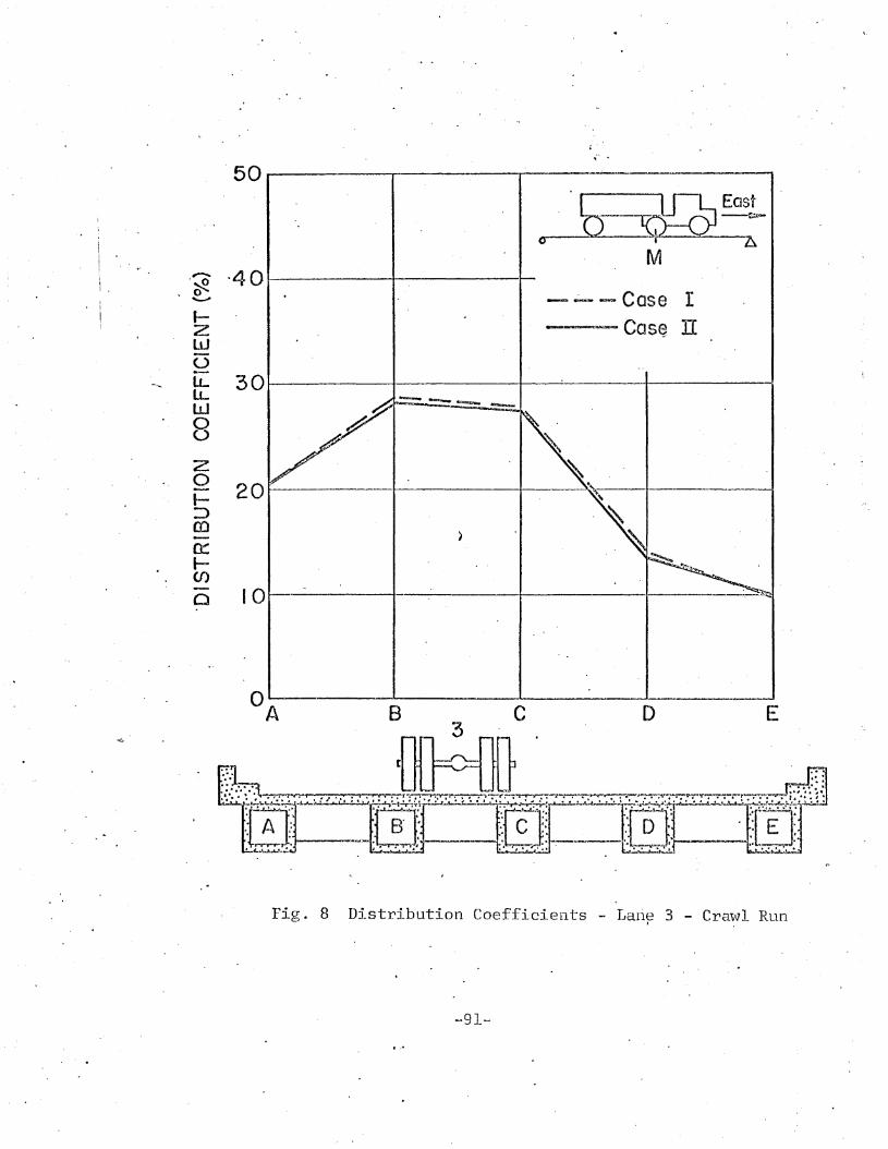
I OJ-----------I -----+-----1·--
IZWULLLLW
8zoJ::>cocr:l-(J)
o
·;- ..50 --------r....------r---"-----..-----a
-40 J-----+-----t--
-.:- - Case I__~.....=m_ Case IT
301--------4--------1----.:..-----+----
2 0 1--"----I-------I-----"'.""~... --t---,----1~
~
Fig. 8 Distribution Coefficients - Lari~ 3 - Cra~l Run
-91-
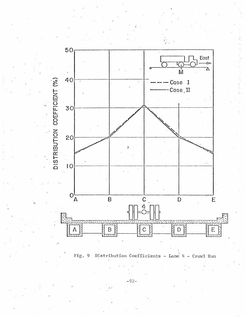
....~. .
"
50
'a [(iID~0
M .,."..-.. 40.. 0 ---,Case I~............
l- Case JJ1zl!J0LL 30LLIII
8Z0 20I-::)
1co0::'l-(f)- 10 --0
Fig. 9 DistribLltion Coefficients - Lane' 4 - Crawl Run
-92-
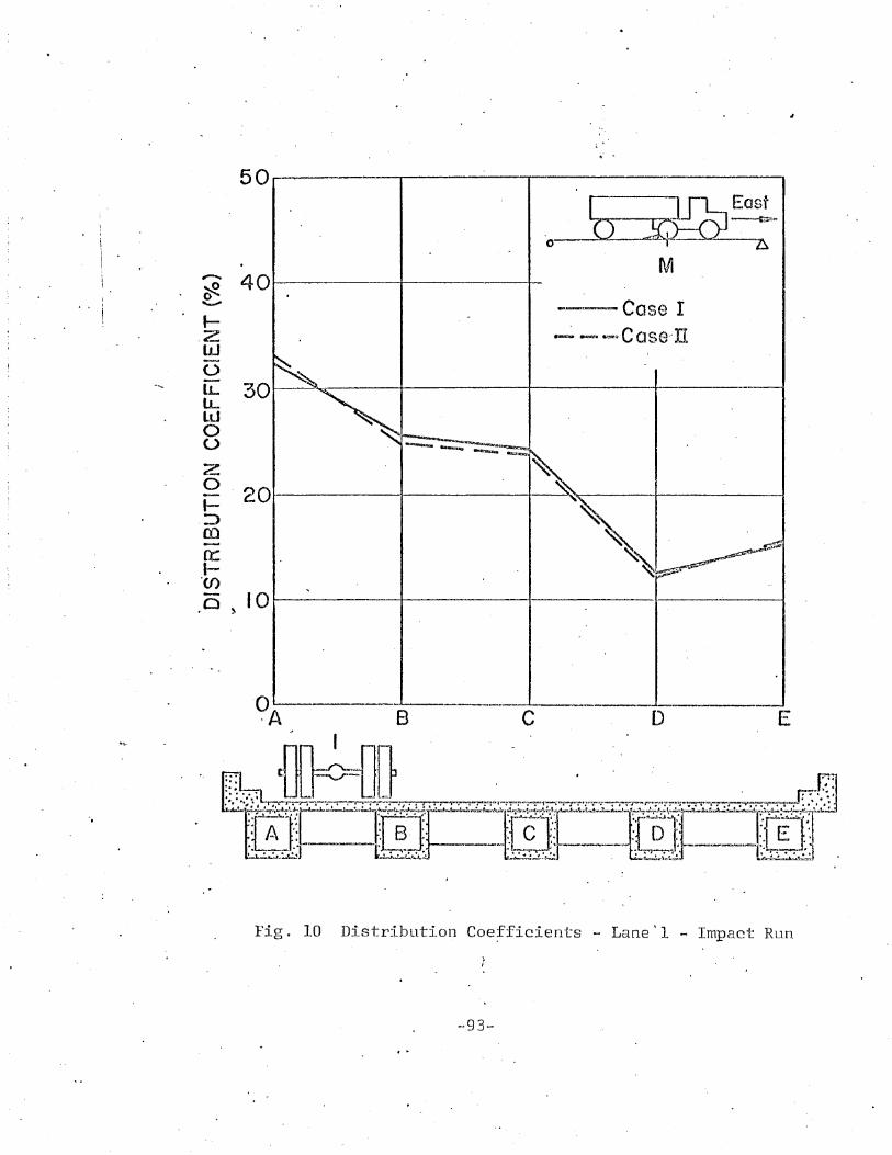
Fig. 10 Distribution Coefficients - Lane'l - Impact Run
-93-
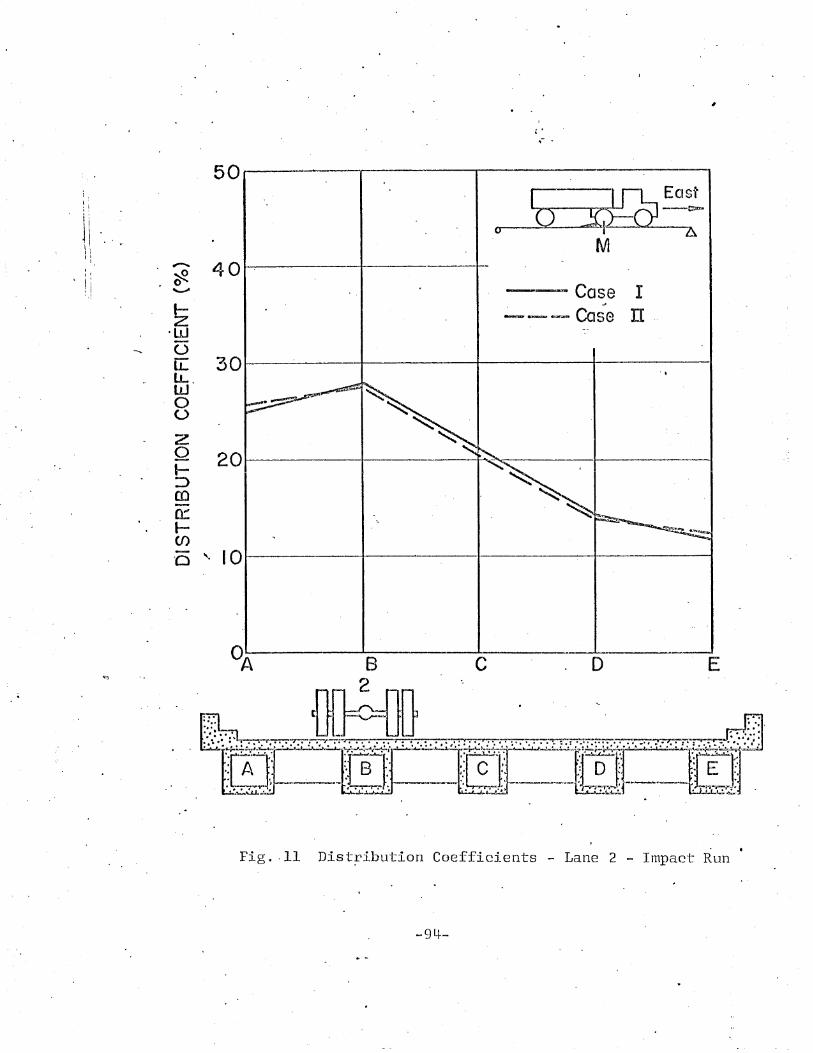
,
50--'-~'-------'-----
......-._~ Case I~ --=- -- Case IT.~
·woLL 301--------I-------f------;------jLL.Wouzo 20 I---~---J.___---~""=:___----r-----____II::>con::I(f)
'0 " I0 J.--------f------t--------t--------j
. ~ 40.. 0.........-
i,
\ i
1 " ..\II
I
Fig .. 11 Dist~ibution Coefficients - Lane 2 - Impact ~un ·
-94--
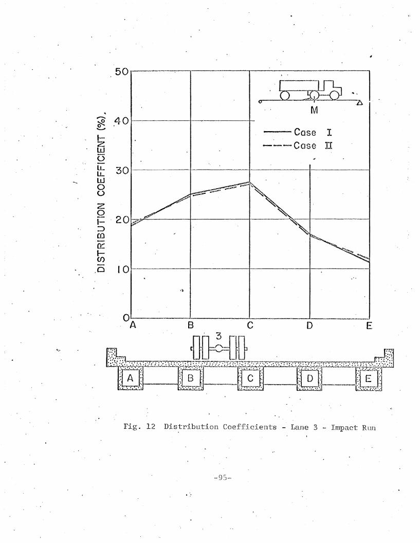
--Case I----- Case IT
50---- .
I-Z·wo& 30w·o -~
() ~~~ ~
~
5 "I- . 2 0 ~~-r.-~----f--------t----~~:JenccI-U)
o I 0 ------)------+-----:-----t-------.......
Fig. 12 Distribution Coefficients - Lane 3 - Impact Run
-95 ....
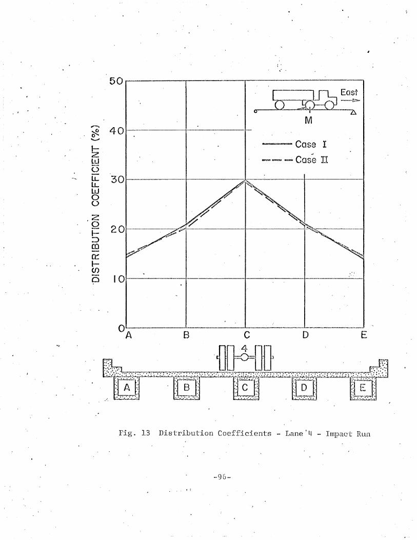
50 _-....----r-------,--------------.
o
~
40~0"'"-'"
l-z·lLi0LL 3'0LLLJJ00
.2Q 201-:::lro-~
I-00Cl 10
-'+l'
8 C D E
,F'ig.. 13 Distribution Coefficients - Lane' 4 - Impact Run
-96-
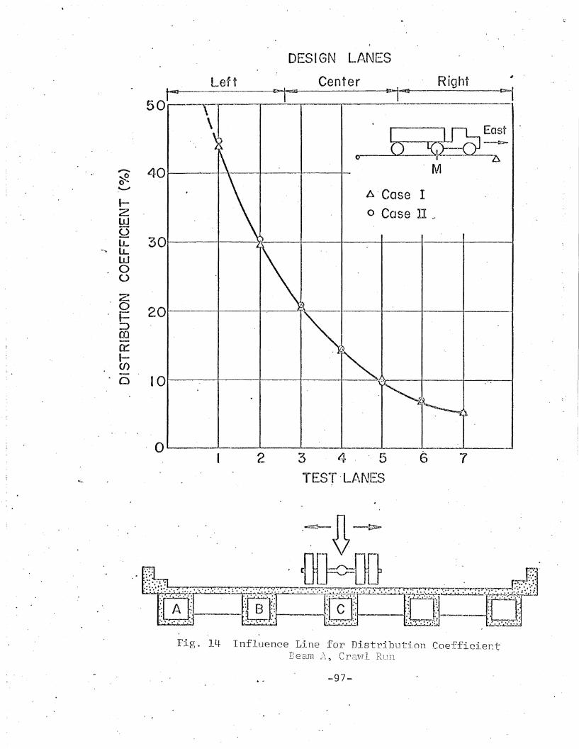
,Right
A'Case I
o Case IT ~
DESIGN LANES
Center
I OJ------f------f----+--..+-·~ O-----+-......----~--I
2 Ol------+----+-:----"'''i'~--t--jr-----r-
40l---~ ....--\---o+------J--;-,,-....
~0.............
l-Zwc>LL-..... lL.W0~)
Z0t-:Jen0=I-({)--0
o~ ..J -'- .... --- --_.. "'.._-'--__.........-1
234 5 6 7TEST'LAr\J.ES
Fig. 14 Influence Line for Distribution Coefficie~t
Ee Elm ;"\, CrEL\\71 F(U.ll
-97-
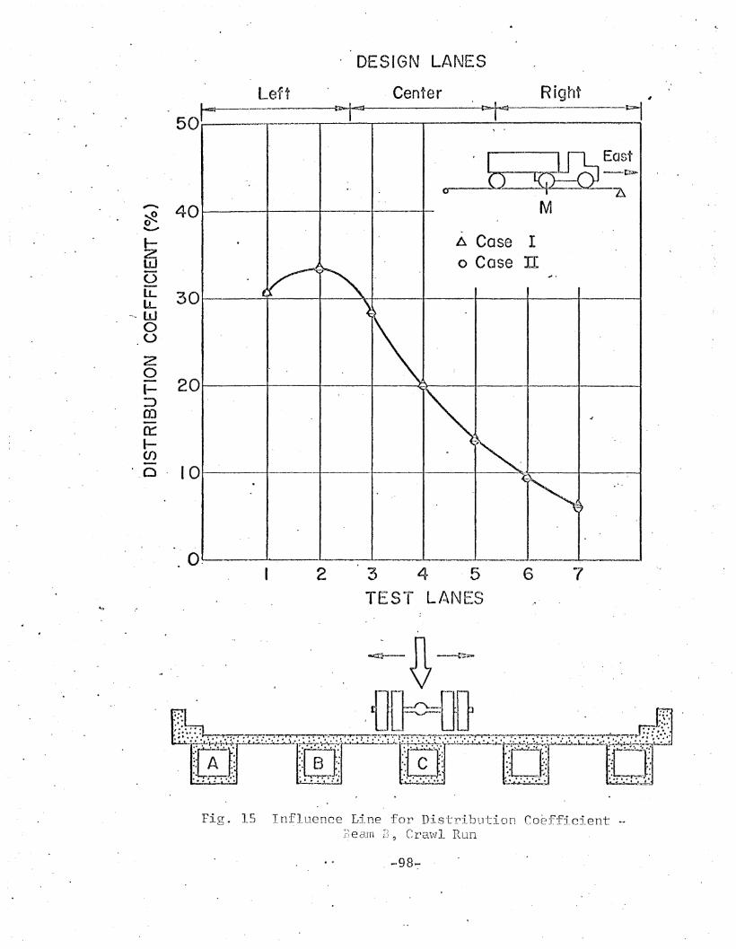
Right
63 4 5TES~'r LANES
. DESIGr\J LANES
Center~- .~
2
--
b J1L6t0Sf.- 0
~ -~, LlM
A Case I---J~ 0 Case JI
....
'"~.
fl- .-)
,
.4'
'" N '.
;"~
-- ,"---,_..=--
20
30
o.
~ 40o.........IzwoLLLL
-'4 WoU
2oI:JOJn-:I(f)-'.0 . 10
Left'50
t---
Fig. 15 Influence Line for Distribution Co~fficient ~eam B, Crawl Run
. -98-:-
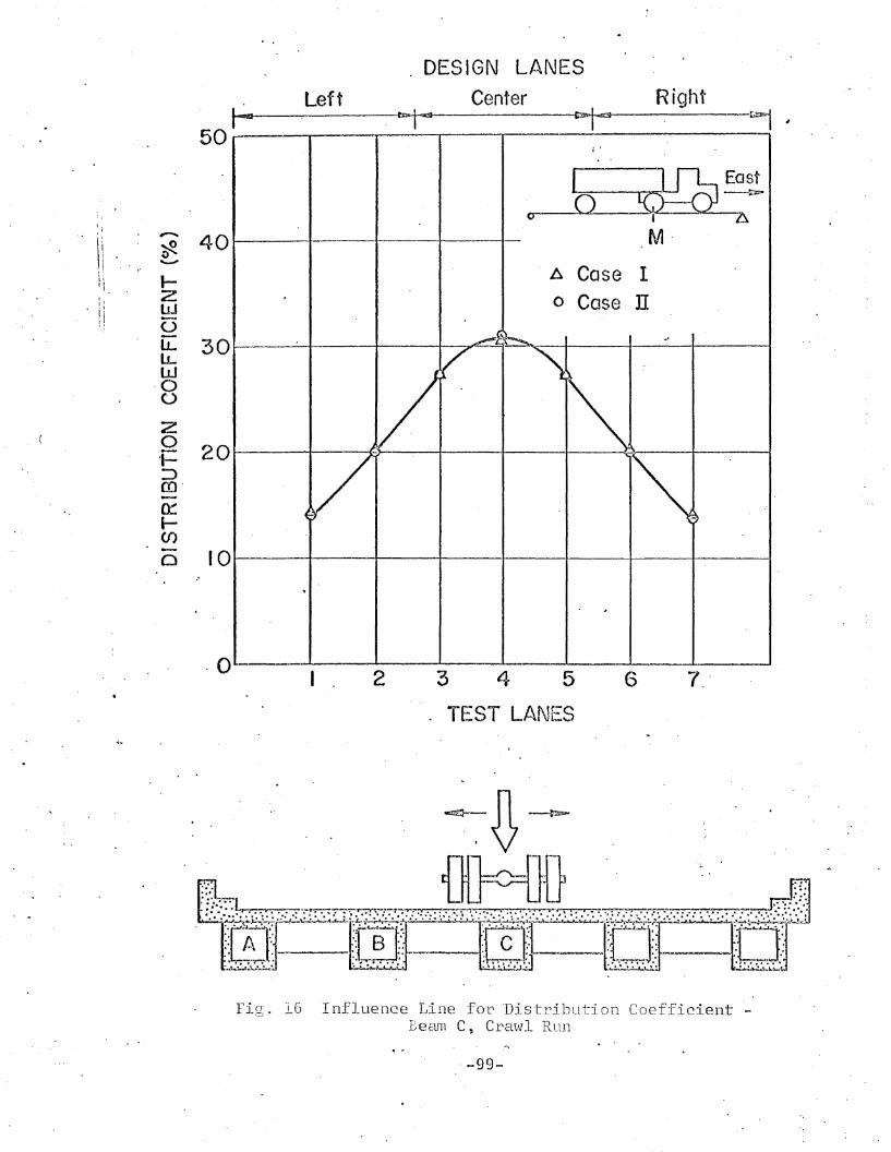
..
J ~:~0
0~A .
A Case 10 Case IT
~b- I ~
(/ ~ ~
).
~V ~-,.
#
50
~
40~n""'--""
I-Zw0LL 30LLW
-00
z0 20'1-:Jco'......-.
0::I-(f')- 100
·0
Left
I. 2
. DESIGN LANES
Center
3 4 5
TEST LANES
6
Right
7,'
Fig. l6 Influence I.line for "Distribution Coeff'icient Bea.nl C, Crawl RUT1
,.....
-99-
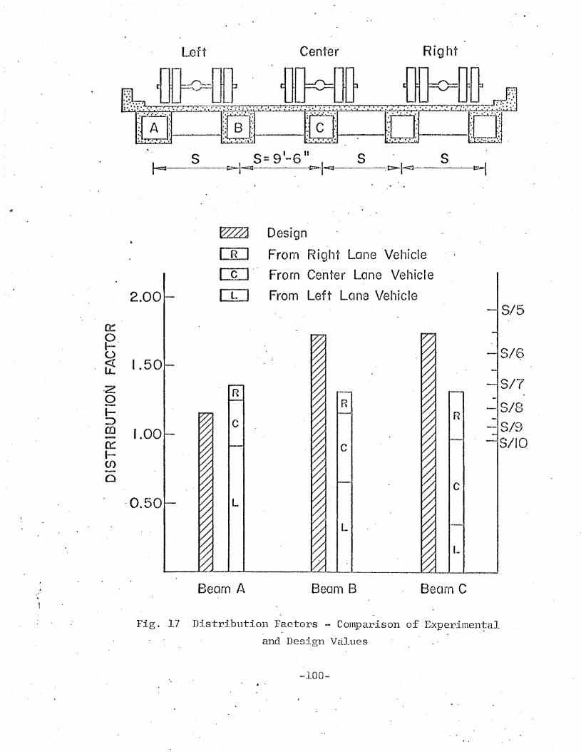
l.eft Center Right
L- S . S=91-6
11S
r----~--· ~--I~~ ~.~--S
~ Design
LID Fronl Rigl1t Lane 'Vef~1icle
G:J" From Center Lane Vet1icle
2.00 CD From Left Lalla Vel,icle8/5
~
~.SIC?()
It 1.50
42-.. s/-r
R0 R -I- -- S/8::> c
R -ro 1.00 -- 8/9- S/IO0:: cI-(J)-0 c
'0.50 L·
I_
t..
,,"
1
Beam A Bean) B Beanl C
Fig. 17 Distribution F~ctors - Comparison of.Experimenta1
and Design-Values
-100-
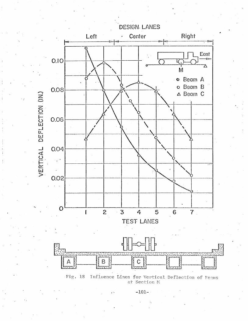
.~
DESIGN. LANES
Left · Cel1i'erral-------:~~
0.1 0 l-----l---\.--l------t----t-
·0 Bearn A
0.08 0 Beam B,.........
6. Bearn CZ /''-""
z~
0I-- 0.06u
\w\._J
lL \-W0 ,.J 0.04 ~<:(
"u-- .1- - 1:'"
~l!J>.
0.02 ----
o2 ·3 4 5 6 7
TEST LANES
. .
,Fig. 18 Influence I,ines for "\lertical Deflection of P,eamsat SectioTl tvI
. -~ -101-.·
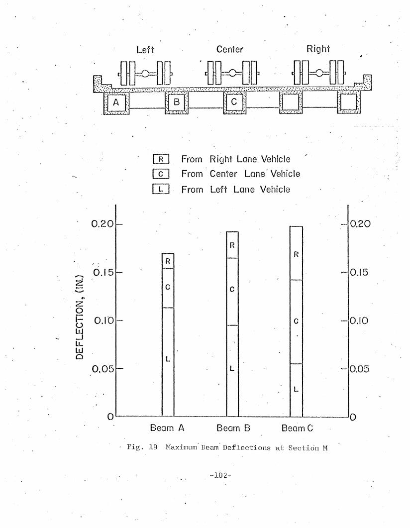
Left Center Right
[[] . From Rigllt Lane Vel1icte-"
~.
m From Center Lan.e· Vet1icle...
. ,
IT] From l.,eft LOf1e Vetlicle
0.20 0.20
Rf~
R
.,........., 0.15 0.15Z c'--'" c~
z0i= 0.10 -- c --- O.tOUl!J-'l'-W0 L
0.05 L 0.05
L
o~---&...~-
Beam A Scorn B
· Fig. 19 Maximum' Beam" Deflections at Secticin M
-102-
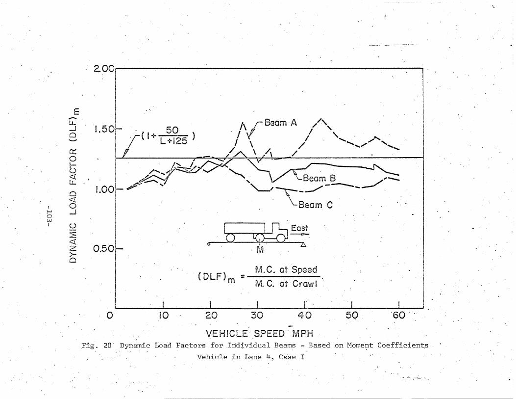
'';'
2.00. i
,. I
I
rt/i. C. at Speed
M~ C. at· Cravi i
"
Beam'A //', ,1\ . /, .' / ......
. I / ' ....... '/ .........I \ // .... '"
",~~.,
" V '-Beam B. '-'~_.-/---_.-/~--
. Beam C . .
I .ld-Q5J East'0 I ~OJ' '2).
·M
'(DLF)m =
1.00
0.50
. \
. J
1.50r.~ 50. , r (I + L +125 )
I
E....-...LL-.J0'-""
0::0~0<J:lL
0<l
! 0f-Ja -iLvI U
::::«z>-c
i .
; I I I L..I I!0' 10 20 30 40 50 . .60 ' '.
-VEHiCLE- SPEED' Iv1PH
,Fig. 20' Dynamic Load Factors for .tnd~vidual Beams - Based .on Mpment Coefficien~s
Vehicle in Lane 4~ Case- T'
• ~ ~ . r" ~...."7"' ~ ~ • ,
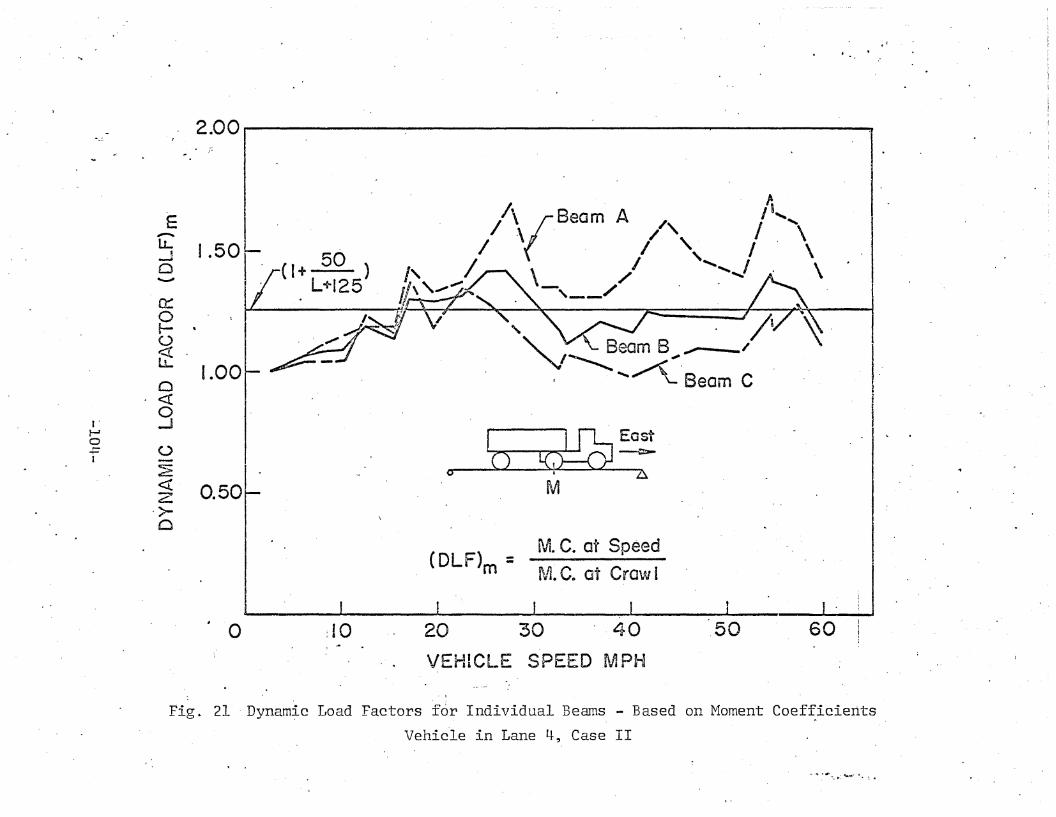
.'
, 2.00. -.
.:
I (DLF)m = M. C. at SpeedL. . M.C. at Crawl
I J_-_------J
E....-..J .50LL
"--Ii
0.........,
a::0f- ..0
it1.00
0«0...Jt·
~
0()r-
-or-I
~« 0.50z
.>-0
~
f\ B A I',/"(. earn //, / "-/ \. I', I· \,
/ r-'\. \ ~I ..............J 4." \
o :10 20 30 ' 40 .50 60.. .
VEHICLE SPEED.M PH
Fig~ 21 'Dynam~c Load Factors for Individual Beams - Based on Moment Coefficients
Vehi~le in Lane 4, Case II
~..... ~ .... p' ,~~~ ..
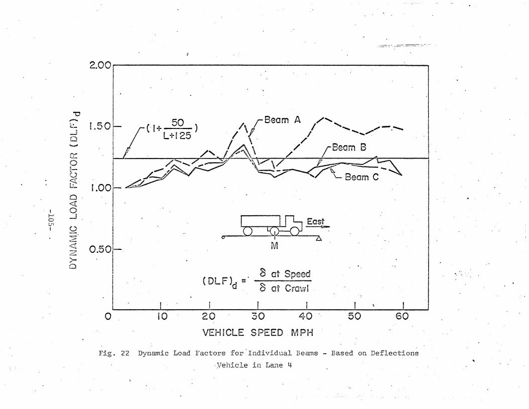
--:::-_-=--==-, ....:...=-=~~ .. _......~---_....
2.00,......,--------------------....
60
'I
5040 .
8 at Speed
3 at Cra\~i .
30
/(seam A /,I
\ ' I............ ""---I ' ......"... .. ---/' / .
~\ // [Beam B I\7 7 ' A I~t# 'IZ:E _ /' c::::=\:
I ~Eosto ~o ~
pJi
(DLFJd ='
I2010o
~,.-.-,..
L50~ (- f+ 50 )iL.J / L+1250 I'
'-"" IG.::0f·-0~.D_ 1.000<!
J 0r -J0LnI 0
:;; Lt:_
<!z 0,.5°
1
.'-.r
0 It
VEHICLE SPEED ~\~PH
Fig. 22 Dynamic Load Factors for 'Individual Beams - Based on Deflections
'Vehicle in Lane 4 "
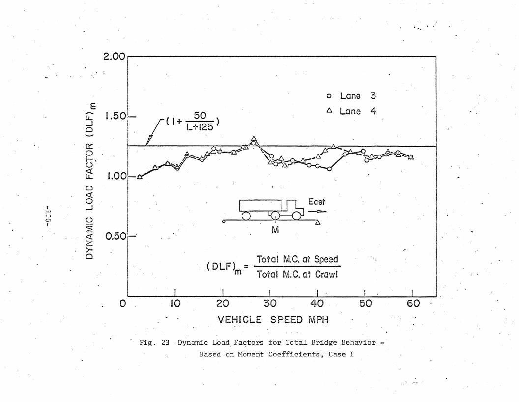
2.00 I
, .
(. , Total M.C. at Speed i~DLF; = _r------
m Total M.C. at Cra\~1
'e,......l1..--l0............
~
01- ..U
it0<t:0...JI
}--1
00m
~1
<!Z>-0
1.50
1.00
0.50
(I + 50I • II'""\~ )
o Lane 3
A Lane 4
I .~~O' Io h
M
,/
o ' 10I
20 30 40 .
VEHICLE SPEED MPH
50 60
Fig. 23 -Dynamic Load, Faqtors for- Tota~ Bridge Behavior
Based on Moment Coefficients, Case I
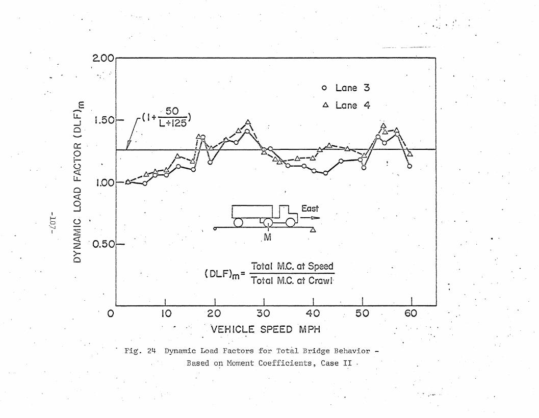
,1
..... t ..
2.00· ·
o Lane 3
/). Lane 4··50
( I + I • ,~,.- )
I.OOr-L_~
1.50'~
cco~o«LL
E,-....
IJ...-l0,
tt-'-o
~-......j
t
o<Cgo·2:~ .0.50>o
I ~ECisto I ~.o 2i.
M
(DLF)m= Total M.e. at Speed
'0 10 -20 30 40
VEH~CLE SPEED 'MPH50 60
. Fig. 24 Dynamic Load Factors for Total Bridge Behavior
Based o~ Moment Coefficients, Case II
~~;, 4"';<"-' ~ •
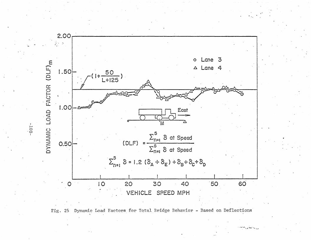
;,
2.00. ,..- ~ ,"
o Lane :3A. Lane 4
5In:, 8 at Speed
c;-
2:~:1 8 at Speed
I ~Easto --"..o fVi h
(DLF) =
50 ).(I+ L+125
1.00
0.50
i .50
E-----LL-la............
cc0t-o
·tt0<:C
'0-..JJ
!-J()0
~ co
~I
<:(Z>-0
. 5 '.l:n: I 8 = L 2 (8A + 8E ) +8s+ 8c+80
~ 0 10 20 30 . -40 "50. 60
VEHICLE SPEED MPH
Fig. 25 Dynamic Load Factors, for· TQtal Bridge Behavior - Based on Deflections"
..... ~'';'''. ;".' 'I40\oI" '1 .. - '-..-...
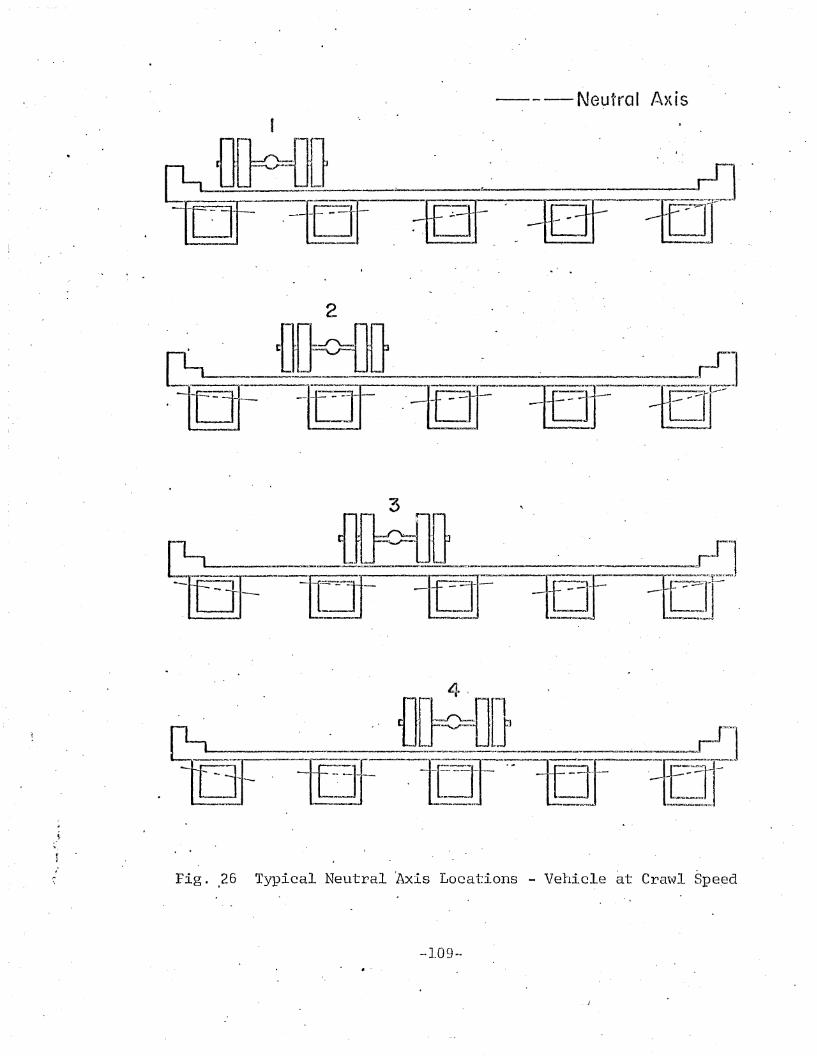
---Neutral A)(isI , J •HJ .' .. '.
'. .
. .
Fig ..26 Typical Neutral Axis Locations - Vehic~e ~t Crawl ~pe~d
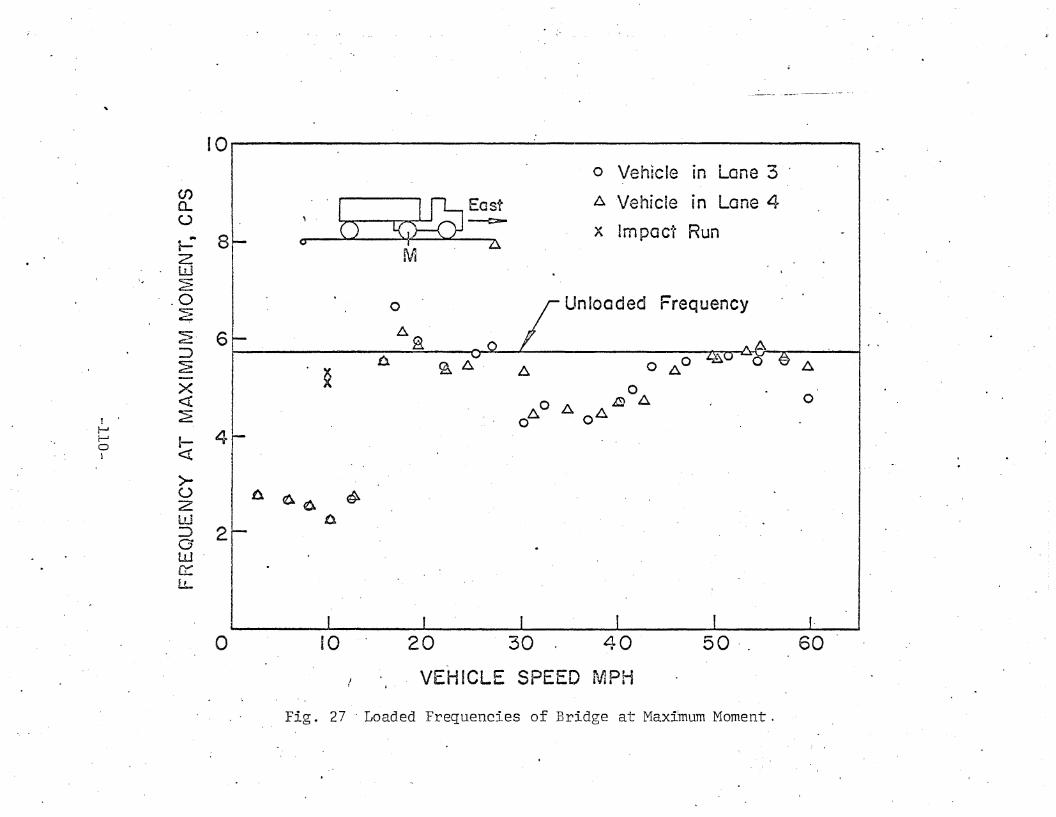
- _._~-- - ....-.---
"\
10I
o Veh~cle in Lane 3(f) . I
~~~ 'Vehicle in Lane 40..
U ,
- 8 0() L( x Impact Run
f- M . 21ZWSot::::...
.0 0 r Unloaded Frequency:?;~. 6 6- a:::> 0. ~ 6.-.~ o AO - V 'J A- . ~ ~
x 0<:(
A O A ~ISJ ~ 0
! . 2: o 01-' 4~ I-a1 <t
>()
ZlJJ
~ 2wG:::U.
b 0-0. ~
0.
o 10 20 30 40 50· . 60
VEHICLE SPEED MPH
Fig. 27 . Loaded Frequencies of Bridge at Maximum Moment.
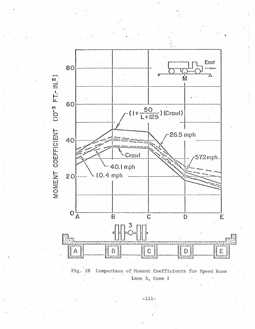
,
801-----·+-------t--
N'.Z
601------+----.1------+---------150 ~
( I +-~-) (CravJI)L+125
26.5 mph
--1--------
40.1 mpl-,10.4 mph
l-ZWoLLlLWoU
~ 20lJJ~o2
;
."-----~~ _._-------~
.Fig. 28 Comparison of Moment Coefficients for Speed Runs
Lane 3, Case I
-111-
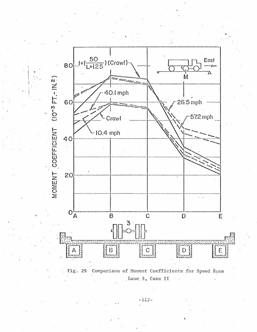
.,
10.4 mp}1
60
IZw 4 0 J.---------J.----.-----f---~
()
LLLLWo
.0
~. 20w~o
'2
~IJ..ro•-·0
I
i
i 0.
I 'I
'.' Fig. 29' Comparis?n of Mornent Coefficients for Sl?eed R~ns
. La11e. 3, Case II'
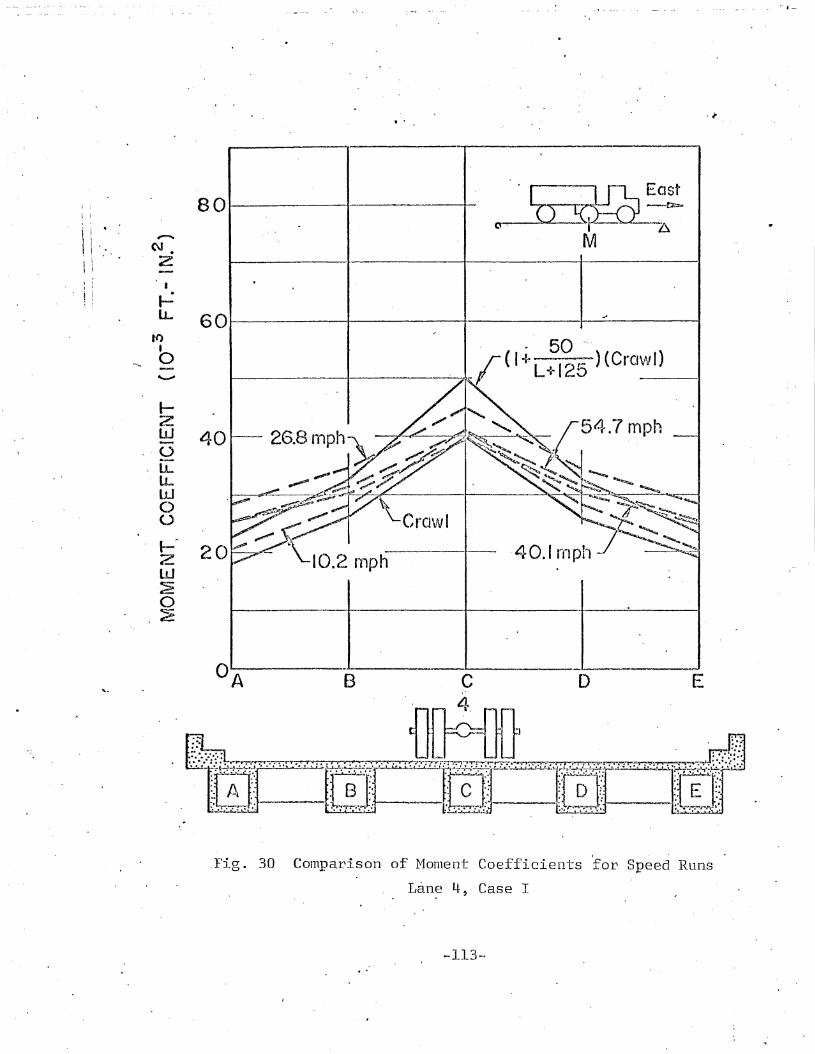
.;
80 [0 ~~( ':
! i
\. 0" I -~,.......... M
1 (\I.
z
J-=I.L 60
1'0 - 50--•0 ( I+.. m3~ ) (Craw I)'-"'" L+125
I-zw 40
.-0LL
"LLW00
I-"~
20 40.1 rnpllzw-~
0c.::=.i!:
O----A----SA-----C'L-·------.L-D-------'E
, 4.~ *} .
::: . ::::.-.. ~ ... . : .~ .::-~
~['AJ~r raf '[~~ ;rtr lE~~~::._~--,,----.~:: ~. -~.. ....-.;o:-,:,.: :;.,-;.-,..,..::
I
,Fig. 30 Comparison of Moment Coefficients for Speed Runs
Lane 4, Case I
-113-~
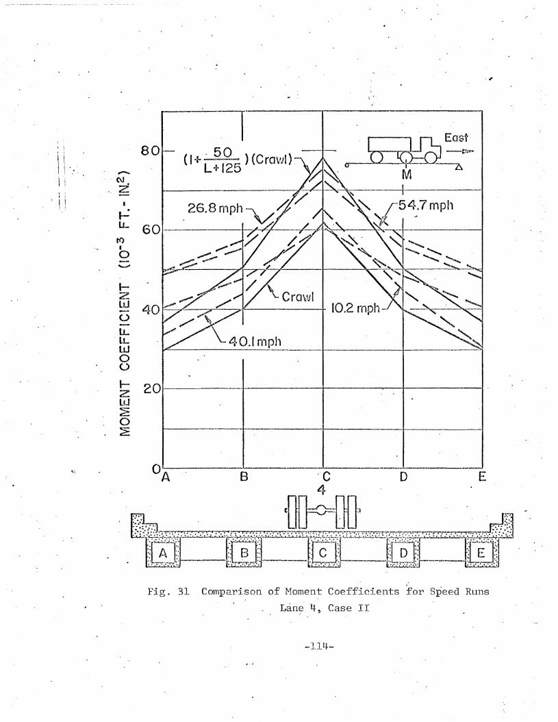
·,.. .
;" .
~.
80(I+d&) (Crawl)
"......,
(\J
(Z
I
. !r:LJ_
60t()I0............
1-Zw 40 10.2 rnph--u-LLLL - 40.1 ~npJlw0U
I-- 20ZltJ~0~
Fig. 31 C0111parison of Moment Coefficients for Speed Runs
JJan~ '4, Case II
-lll~-
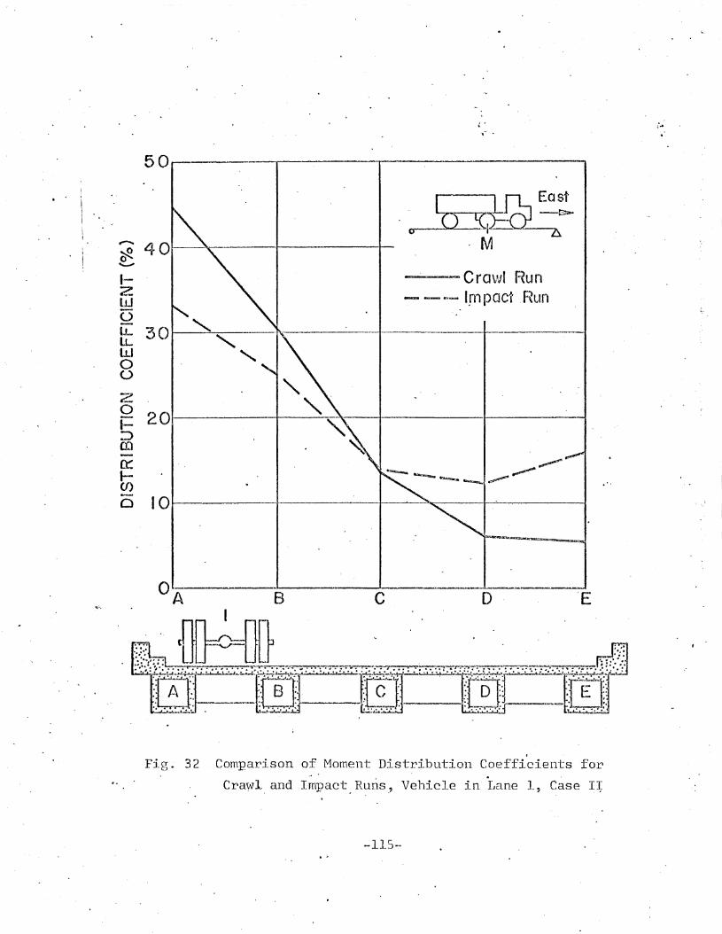
I· t ..•",..
50
1(;~0...--.. 40 ·M~0'-"""
I- =- CravJI Runz
--- - -- (~m ()Qct _Runw0
"'-LL 30LL "'-LLI "-0()
z0 20l-::)D:l-0: ~~I- ~~---=..~ ."(f)
Cl 10
B C~-_..
o
I
Fig~ 32 Comparison of Moment Distribution Coefficients for,. . .
Crawl and Impact Runs, Vehicle in Lane 1, Case I~
-115-
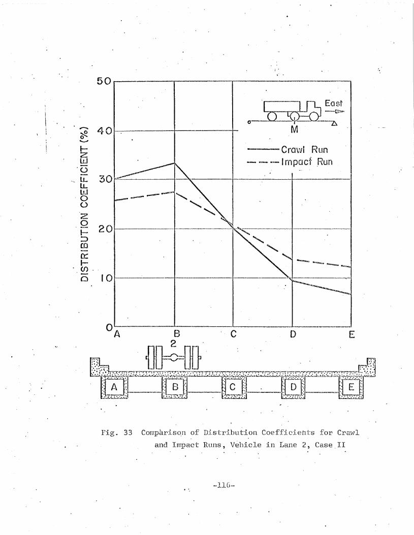
50 ------....,....-..------.-----------.
I,\ ,
o~ 401--,--_'--';"'-1----'-'
o'-"
.a=bU Cro\vl RLJn- ~ -Irnpacf ,Run
IZW
'U___ LL 30pc..------t-~---_t__
1..LLLJ
'0oz
.QI- 20::>en~l-. (() ~ .
o IOJ.------t--------+-----~f
". C D E
Fig. 33 Comparis~n of Distribution Coefficiehts for Crawl
and Impact Runs, Vehicle in -Lane 2, Case II
-116-
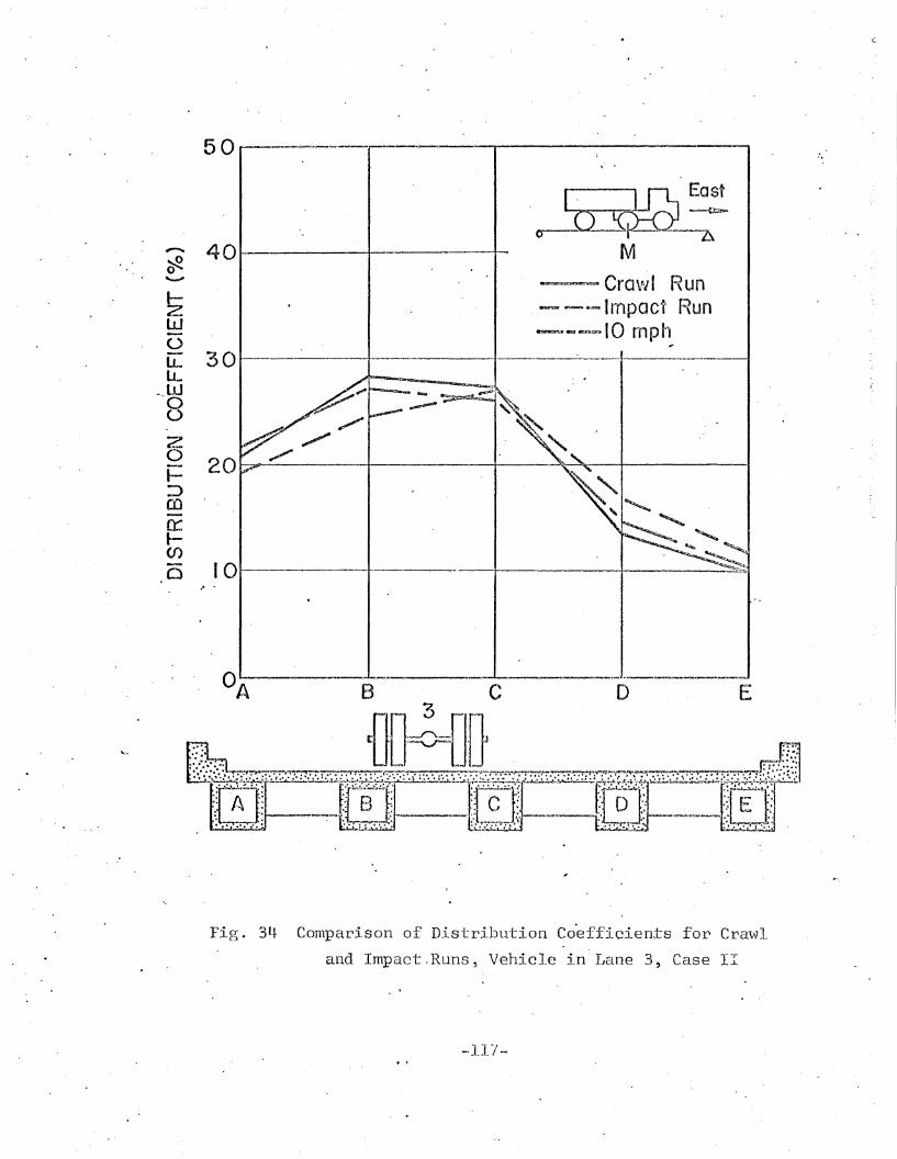
50" .
,,-.... 40~0.' ..........,
I-2:W()
LL 30Lt_
_ llJ
8Z0 20I-::>co0::~-(J)
0 10
o10~7M
~~- Crav/l Run, --=--~ Irnpact Run~oa&fl~~IO mplp)
' .--L-... ~_,~__ ,-...-.-..-...-..1
Fig. 34 Comparison of Distriblltion Co·ef~i~ien:ts for Cra\vl
and Impact.Runs, Vehicle in Lane 3, Case II
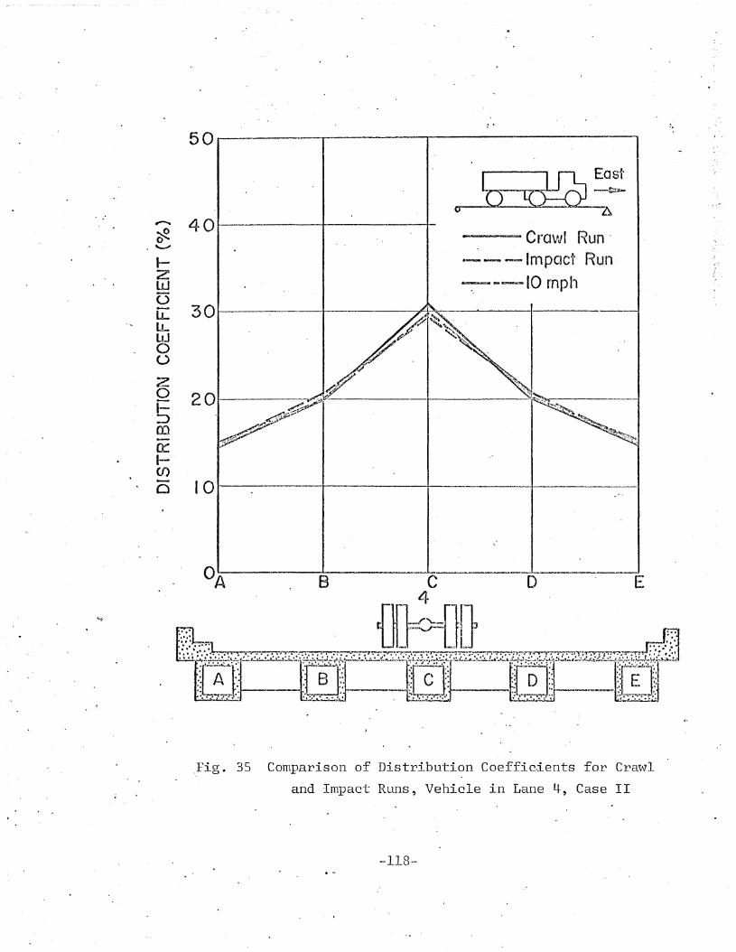
50 _---,-..-,--------r------------,
IOI------t------t--------I------1
..........__s:::aa;;:-.;:c_ CravJI Run'
·--~ln1pQct Run~--=IOmpI1
o
30t--------t-------;P-1. :lIk--------f----
4 O~---t-------t
,.ZlJJ()
LLLLlJJoU
Zot::>CO0::tOO
~O
. 8 C--..------[)·4·
E
.Fig. 35 Comparison of Distribution Coeffic.ients for Crawl
and Impact Runs, Vehicle in Lane 4, Case II
-118-
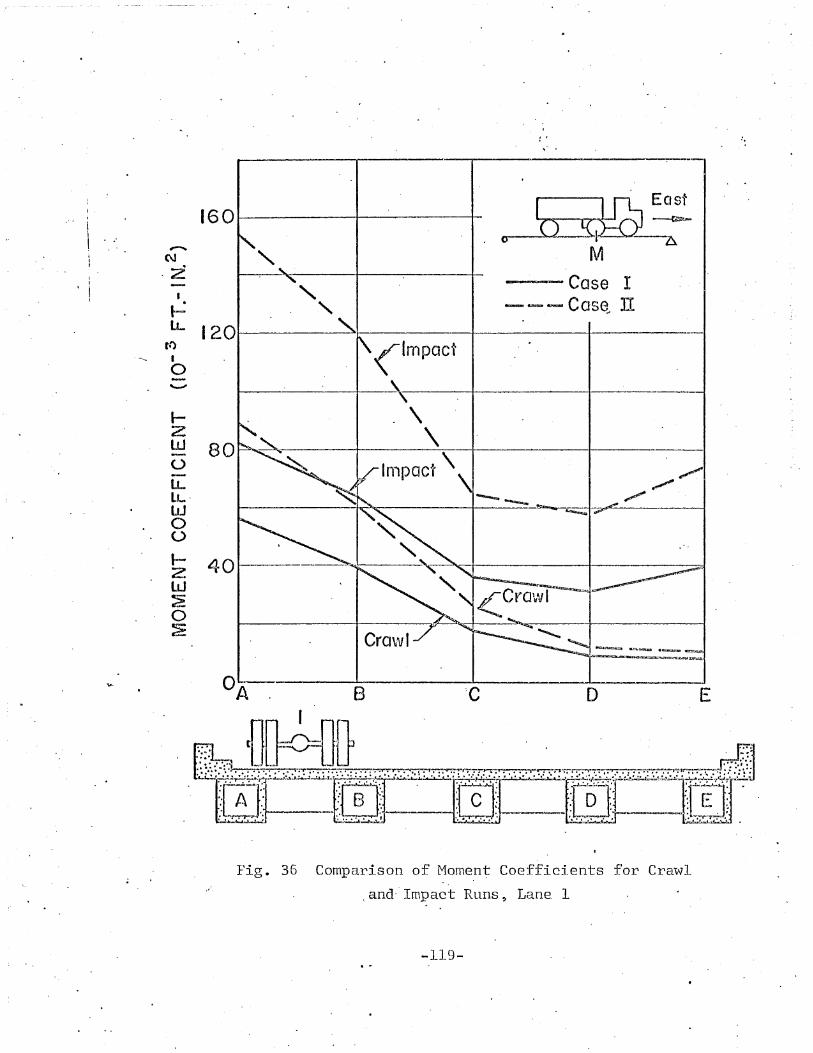
",.' .
r~ rl-,~0-.---1) ~~
I\~
---Case I-- -- - Ca'se~ n
Cro\vl
(Impact
.------+--\--t--------f---.\
\80
4 0 t--------~"---
IZW()-LLLLLJJo
~U
I2W~o2
160• * ,.........
"N
I ·2 ,t
\ \ "f~,
LL 120f:)
I
0"'-'"
Fig. 36 Campa,rison of Moment Coefficients for Crawl
"and- Impact RllllS, Lane. 1
-119-
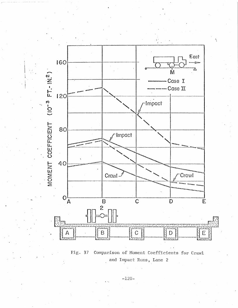
I
Impact
il r~. East
c-U CC}BY-7M .
~Case I
-----Case JI
I2W 80~-----f-----------t---~--t-----t
()
IJ_LLltJoU
I- 4~0ZLLJ2
-0~
160. .
,-...\ C\JI .
-2
~ .--=-~ ",..."..,.
LL 120ft) "--. I "0
............
Fig. 37 Comp~rison of Moment Coefficients 'for Crawl
B.nd Impact Runs, Lane 2
-120-
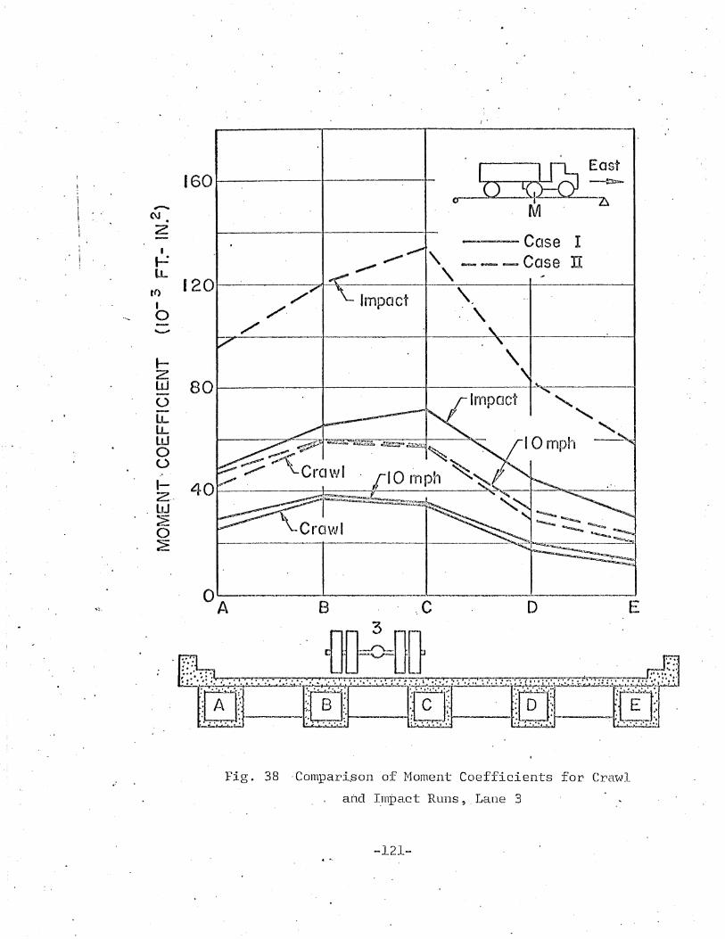
\
'\
Impact
o
Impact
tt=~~. M. "b.
~--Case I" --~ -- Case IT." ~
.-----'------:.~----__t_
\4\
\
160.......-...
(\J .Z
I
t-=LL
tf> 120I
,/
0 /'-....-.. /
I-Zw 80uLLLLlLf0U..I- 40z ..
. W20~
oA 8.C D E
..,· . {l[}~{}[} .. '"
:~. ~ --tG..!.i rI) \.?,*t ~.!.
Fig. 38 ·Compari,son of Moment Coefficients for Crawl
and I.rnpact Runs, Larle 3
-121-
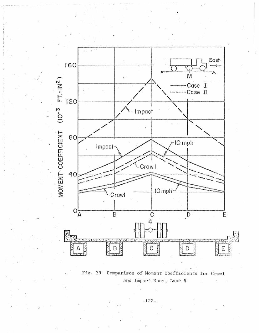
---,.,.,.-..__--......-_------.---------
""
.
M
~". -Case I" -----~Case II
"/
/
/Almpact
""-----J.-----f-----------"
0,A..----·.L__------",B C
4- .
~.~=:~ . t!JOr<;::JL,JOJ Jm':'.:'.,:~ -= ... ':::":...;:
'. ". • •. · .... ;. 'Yc..:.,.r.l .1"n-f':";i • ..~•••. ;",.. J.... .. ~oiIIIII= ~__.,.... ... ~~.,.II:;.L
160
~ ~.
,,-....
..' NZ
I
~LL 120
toI
0'"'-'""
/'J- /
Z 80LJJ0LLLLW0<->I-.~
. ~20'~
, .
Fig. 39 CompariS011 of tvJoment Coefficients for Craw]_
aQd Impact Runs, Lan~ 4
-122-....
.1
11. REFERENCES
1. American Association of State Highway OfficialsSTANDARD SPECIFICATIONS FOR l-IIGHWAY BRIDGES,Washington, D. C., 1965.
2. Pennsylvania Department of Highways, Bridge DivisionSTANDARDS FOR PRESTRESSED CONCRETE BRIDGES,ST200-ST208, 1964.
3. Douglas, W. J. and VanHorn, D. A.LATERAL DISTRIBUTION OF STATIC LOADS·IN A PRESTRESSEDCONCRETE BOX-BE~1 BRIDGE, DREHERSVILLE BRIDGE;Fritz Engineering Laboratory Report No. 315.1,Lehigh University, August, 1966. '
4. Guilford, A. A. and VanI-lorn, D. A. .LATERAL DISTRIBUTION OF DYNAMIC LOADS IN A PRESTRESSEDCONCRETE BOX-BEAM BRIDGE, DREHERSVII1LE BRIDGE,Fritz Engineering Laboratory Report No. 315.2,Lehigh University, February, 1967.
5. Guilfor,d, A. A. and VanHorn, D. A.lATERAL DISTRIBUTION OF VEHICULAR LOADS IN A PRESTRESSED··CONCRETE BOX-BEAM BRIDGE, BERWICK BRIDGE, Fritz Engineering Laboratory Report No. 315.4, Lehigh University,October, 1967.
6. Schaffer, ThoInas and Van}Iorn, D. A. .STRUCTURAL RESPONSE OF A 45° SI<E\v PRESTRESSED. CONCRETEBOX~GIRDER HIGHWAY BRIDGE SUBJECTED TO VEHICULAR LOADING,BROQI<VILLE BRIDGE, Fri tz Engineering La]Joratory· ReportNo. 315.5, Lehigh University, Octobe~, 1967.
7. Lin, C. S. and VanHorn, D. A.THE EFFECT OF MIDSPAN DIAPHRAGM ON LOAD DISTRIBUTION INA PRESTRESSED CONCRETE BOX-BE~l, PHILADELPHIA BRIDGE,Fritz Engineering. Laboratory Report No. 315.6, LehighUniversity~ June, 1968.
-123-
8. Guilford, A. A. and VanHorn, D. A.LATERAL DISTRIBUTION OF VErIICULAR LOADS IN A PRESTRESSEDCONCRETE BOX-BEAM BRIDGE, WHITE tffiVEN BRIDGE,'.Fritz Engineering Laboratory Report No. 315.7,Lehigh University, August, 1968.
9. VanHorn, D. A.STRUCTURAL BEHAVIOR CHARACTERISTICS .OF PRESTRESSED .CONCRETE BOX-BEAM BRIDGES, Fritz Engineering LaboratoryRepor-t No. 315.8, Lehigh Dniversi ty, December, 196.9.
10. Motarjemi, D.THEORETICAL ANALYSIS OF LOAD DISTRIBUTION IN 'PRESTRESSEDCONCRETE BOX-BEAM BRIDGES, Ph.D. Dissertation, LehighUniversity, October, 1969.
11. Linger, D. A. and Hulsbos, C. L.DYNAMICS OF HIGHWAY BRIDGES, Iowa State HighwayCommission, Iowa Highway Research Board, BulletinNo. 17, November, 1960.
12. Biggs, J. M., Suer, H. S., and LOlIW, J. M.VIBRATIONS OF SIMPLE-SPAN HIGIDvAY BRIDGES, Transactionsof American Society of Civil Engineers, Vol. 124~ '1959.
13.. Louw, J. M.THE VIBRATION OF TWO-·SPAN AND SIMPLE-SPAN HIGillNAYBRIDGES, The Civil Engineer in South Africa, Vol. 5,No. 12, December, 1963. .
14. Varney, R. F. and Galambos, C. F.FIELD DYNAMIC LOADING STUDIES OF HIGHWAY BRIDGES INTHE U. S., 1948-1965, Highway Research Record, No. 76,Highway Research Board of the National AcadenlY ofSciences - National Research Council, Publication 1261,1965.
15•.Fang, Shu-jin, MaJias Rend~n, M. A., and VanHorn, D. A.ESTIMATION OF BENDING MOMENTS IN BOX-BEAM BRIDGES USINGCROSS-SECTIONAL DEFLECTIONS , Fritz Engineeri11g LaboratoryReport No. 322.2, Lehigh University, June, 1968.
-124-
T ,16. Macias Rendon, M. A.
A STRUCTURAL MODEL'STUDY OF LOAD DISTRIBUTION INBOX-BEAM BRIDGES, Ph.D. Dissertation, LehighUniversity, May, 1968.
17. Sanders, W•.W. and Elleby, H. A.DISTRIBUTION OF WHEEL LOADS ON HIGtfivAY BRIDGES,Engineering Research Institute Report No. 361, .Iowa State University~ Ames, Iowa, December, '1968.
18. Varney, Robert F.THE DYNAMIC BEHAVIOR OF A SINGLE SPAN PRESTRESSEDCONCRETE BOX-BEAM HIGHWAY BRIDGE, Fritz EngineeringLaboratory Report No. 315.4ST.
19. Kinnier, H. L. and McKeel, W. T.A DYNAMIC STRESS STUDY OF THE HAZEL RIVER BRIDGE,Virginia Council of Highway Investigation andResearch, 1965.
20. American Concrete InstituteBUILDING CODE REQUIRE~1ENTS FOR REINFORCED CONCRETE,ACI Standard, ACI 318-63, 1963.
21. Prestressed C011crete InstitutePRESTRESSED CONCRETE BUILDING CODE REQUIREMENT, 1961.
-125-

12. VITA
Yan-Liang Chen was born on August 28, 1940 in Tou-Liu,
tTaiwan, China as the third child of Ts uan-Ti and Yu-lu Chen. His
parents are doctors and have four sons.
He received his high school diploma from the High School
of National Taiwan Normal University, Taipei, in July 1959. Four
years later he graduated from Chung-Yuan Christian College of
Science. and Engineering, Chung-Li, Taiwan, with the B.S. degree in
Civil Engineering.
After one year of military service in the Air Force
Engineering Regiment, and one year worl<ing at Chung-Tai Architect
Office, Taipei~ he went to Japan. In March 1968, he received the
degree Master of Engineering in Civil Engineering from Waseda
University, Tokyo, Japan.'
In the fall of 1968, he entered the Graduate School in
the Department of .Civil Engineering at Lehigh University to pursue
anM.S. degree, and worked ~s a half-time research assistant in
Fritz Engineering Laboratory.
-126-