LeGO-LOAM: Lightweight and Ground-OptimizedLidar Odometry and Mapping on Variable Terrain

Tixiao Shan and Brendan Englot

©2018 IEEE. Personal use of this material is permitted. Permission from IEEE must be obtained for all other uses, in any current or future media,including reprinting/republishing this material for advertising or promotional purposes, creating new collective works, for resale or redistribution to serversor lists, or reuse of any copyrighted component of this work in other works.

Abstract— We propose a lightweight and ground-optimizedlidar odometry and mapping method, LeGO-LOAM, for real-time six degree-of-freedom pose estimation with ground ve-hicles. LeGO-LOAM is lightweight, as it can achieve real-time pose estimation on a low-power embedded system. LeGO-LOAM is ground-optimized, as it leverages the presence of aground plane in its segmentation and optimization steps. Wefirst apply point cloud segmentation to filter out noise, andfeature extraction to obtain distinctive planar and edge features.A two-step Levenberg-Marquardt optimization method thenuses the planar and edge features to solve different componentsof the six degree-of-freedom transformation across consecutivescans. We compare the performance of LeGO-LOAM with astate-of-the-art method, LOAM, using datasets gathered fromvariable-terrain environments with ground vehicles, and showthat LeGO-LOAM achieves similar or better accuracy with re-duced computational expense. We also integrate LeGO-LOAMinto a SLAM framework to eliminate the pose estimation errorcaused by drift, which is tested using the KITTI dataset.

I. INTRODUCTION

Among the capabilities of an intelligent robot, map-building and state estimation are among the most fundamen-tal prerequisites. Great efforts have been devoted to achiev-ing real-time 6 degree-of-freedom simultaneous localizationand mapping (SLAM) with vision-based and lidar-basedmethods. Although vision-based methods have advantagesin loop-closure detection, their sensitivity to illumination andviewpoint change may make such capabilities unreliable ifused as the sole navigation sensor. On the other hand, lidar-based methods will function even at night, and the highresolution of many 3D lidars permits the capture of thefine details of an environment at long ranges, over a wideaperture. Therefore, this paper focuses on using 3D lidar tosupport real-time state estimation and mapping.

The typical approach for finding the transformation be-tween two lidar scans is iterative closest point (ICP) [1]. Byfinding correspondences at a point-wise level, ICP aligns twosets of points iteratively until stopping criteria are satisfied.When the scans include large quantities of points, ICP maysuffer from prohibitive computational cost. Many variantsof ICP have been proposed to improve its efficiency andaccuracy [2]. [3] introduces a point-to-plane ICP variant thatmatches points to local planar patches. Generalized-ICP [4]proposes a method that matches local planar patches fromboth scans. In addition, several ICP variants have leveragedparallel computing for improved efficiency [5]–[8].

T. Shan and B. Englot are with the Department of Mechanical Engineer-ing, Stevens Institute of Technology, Castle Point on Hudson, Hoboken NJ07030 USA, {TShan3, BEnglot}@stevens.edu.

Feature-based matching methods are attracting more at-tention, as they require less computational resources by ex-tracting representative features from the environment. Thesefeatures should be suitable for effective matching and invari-ant of point-of-view. Many detectors, such as Point FeatureHistograms (PFH) [9] and Viewpoint Feature Histograms(VFH) [10], have been proposed for extracting such featuresfrom point clouds using simple and efficient techniques. Amethod for extracting general-purpose features from pointclouds using a Kanade-Tomasi corner detector is introducedin [11]. A framework for extracting line and plane featuresfrom dense point clouds is discussed in [12].

Many algorithms that use features for point cloud reg-istration have also been proposed. [13] and [14] present akeypoint selection algorithm that performs point curvaturecalculations in a local cluster. The selected keypoints arethen used to perform matching and place recognition. Byprojecting a point cloud onto a range image and analyzingthe second derivative of the depth values, [15] selects featuresfrom points that have high curvature for matching andplace recognition. Assuming the environment is composedof planes, a plane-based registration algorithm is proposedin [16]. An outdoor environment, e.g., a forest, may limit theapplication of such a method. A collar line segments (CLS)method, which is especially designed for Velodyne lidar, ispresented in [17]. CLS randomly generates lines using pointsfrom two consecutive “rings” of a scan. Thus two line cloudsare generated and used for registration. However, this methodsuffers from challenges arising from the random generationof lines. A segmentation-based registration algorithm is pro-posed in [18]. SegMatch first applies segmentation to a pointcloud. Then a feature vector is calculated for each segmentbased on its eigenvalues and shape histograms. A randomforest is used to match the segments from two scans. Thoughthis method can be used for online pose estimation, it canonly provide localization updates at about 1Hz.

A low-drift and real-time lidar odometry and mapping(LOAM) method is proposed in [19] and [20]. LOAMperforms point feature to edge/plane scan-matching to findcorrespondences between scans. Features are extracted bycalculating the roughness of a point in its local region.The points with high roughness values are selected as edgefeatures. Similarly, the points with low roughness valuesare designated planar features. Real-time performance isachieved by novelly dividing the estimation problem acrosstwo individual algorithms. One algorithm runs at high fre-quency and estimates sensor velocity at low accuracy. Theother algorithm runs at low frequency but returns high-

accuracy motion estimation. The two estimates are fusedtogether to produce a single motion estimate at both highfrequency and high accuracy. LOAM’s resulting accuracy isthe best achieved by a lidar-only estimation method on theKITTI odometry benchmark site [21].

In this work, we pursue reliable, real-time six degree-of-freedom pose estimation for ground vehicles equippedwith 3D lidar, in a manner that is amenable to efficientimplementation on a small-scale embedded system. Sucha task is non-trivial for several reasons. Many unmannedground vehicles (UGVs) do not have suspensions or powerfulcomputational units due to their limited size. Non-smoothmotion is frequently encountered by small UGVs driving onvariable terrain, and as a result, the acquired data is oftendistorted. Reliable feature correspondences are also hard tofind between two consecutive scans due to large motionswith limited overlap. Besides that, the large quantities ofpoints received from a 3D lidar poses a challenge to real-timeprocessing using limited on-board computational resources.

When we implement LOAM for such tasks, we can obtainlow-drift motion estimation when a UGV is operated withsmooth motion admist stable features, and supported by suf-ficient computational resources. However, the performanceof LOAM deteriorates when resources are limited. Due tothe need to compute the roughness of every point in a dense3D point cloud, the update frequency of feature extraction ona lightweight embedded system cannot always keep up withthe sensor update frequency. Operation of UGVs in noisyenvironments also poses challenges for LOAM. Since themounting position of a lidar is often close to the ground ona small UGV, sensor noise from the ground may be a constantpresence. For example, range returns from grass may resultin high roughness values. As a consequence, unreliable edgefeatures may be extracted from these points. Similarly, edgeor planar features may also be extracted from points returnedfrom tree leaves. Such features are usually not reliable forscan-matching, as the same grass blade or leaf may not beseen in two consecutive scans. Using these features may leadto inaccurate registration and large drift.

We therefore propose a lightweight and ground-optimizedLOAM (LeGO-LOAM) for pose estimation of UGVs incomplex environments with variable terrain. LeGO-LOAMis lightweight, as real-time pose estimation and mappingcan be achieved on an embedded system. Point cloud seg-mentation is performed to discard points that may representunreliable features after ground separation. LeGO-LOAMis also ground-optimized, as we introduce a two-step opti-mization for pose estimation. Planar features extracted fromthe ground are used to obtain [tz, θroll, θpitch] during thefirst step. In the second step, the rest of the transformation[tx, ty, θyaw] is obtained by matching edge features extractedfrom the segmented point cloud. We also integrate the abilityto perform loop closures to correct motion estimation drift.The rest of the paper is organized as follows. Section IIintroduces the hardware used for experiments. Section IIIdescribes the proposed method in detail. Section IV presentsa set of experiments over a variety of outdoor environments.

(a) Jackal UGV (b) System overview

Fig. 1: Hardware and system overview of LeGO-LOAM.

II. SYSTEM HARDWARE

The framework proposed in this paper is validated usingdatasets gathered from Velodyne VLP-16 and HDL-64E 3Dlidars. The VLP-16 measurement range is up to 100m withan accuracy of ± 3cm. It has a vertical field of view (FOV)of 30◦(±15◦) and a horizontal FOV of 360◦. The 16-channelsensor provides a vertical angular resolution of 2◦. Thehorizontal angular resolution varies from 0.1◦ to 0.4◦ basedon the rotation rate. Throughout the paper, we choose a scanrate of 10Hz, which provides a horizontal angular resolutionof 0.2◦. The HDL-64E (explored in this work via the KITTIdataset) also has a horizontal FOV of 360◦ but 48 morechannels. The vertical FOV of the HDL-64E is 26.9◦.

The UGV used in this paper is the Clearpath Jackal. Pow-ered by a 270 Watt hour Lithium battery, it has a maximumspeed of 2.0m/s and maximum payload of 20kg. The Jackalis also equipped with a low-cost inertial measurement unit(IMU), the CH Robotics UM6 Orientation Sensor.

The proposed framework is validated on two computers:an Nvidia Jetson TX2 and a laptop with a 2.5GHz i7-4710MQ CPU. The Jetson TX2 is an embedded computingdevice that is equipped with an ARM Cortex-A57 CPU. Thelaptop CPU was selected to match the computing hardwareused in [19] and [20]. The experiments shown in this paperuse the CPUs of these systems only.

III. LIGHTWEIGHT LIDAR ODOMETRY AND MAPPING

A. System Overview

An overview of the proposed framework is shown inFigure 1. The system receives input from a 3D lidar andoutputs 6 DOF pose estimation. The overall system is dividedinto five modules. The first, segmentation, takes a singlescan’s point cloud and projects it onto a range image forsegmentation. The segmented point cloud is then sent tothe feature extraction module. Then, lidar odometry usesfeatures extracted from the previous module to find thetransformation relating consecutive scans. The features arefurther processed in lidar mapping, which registers them toa global point cloud map. At last, the transform integrationmodule fuses the pose estimation results from lidar odometryand lidar mapping and outputs the final pose estimate. Theproposed system seeks improved efficiency and accuracy forground vehicles, with respect to the original, generalizedLOAM framework of [19] and [20]. The details of thesemodules are introduced below.

Fig. 2: Feature extraction process for a scan in noisy environment.The original point cloud is shown in (a). In (b), the red points arelabeled as ground points. The rest of the points are the points thatremain after segmentation. In (c), blue and yellow points indicateedge and planar features in Fe and Fp. In (d), the green and pinkpoints represent edge and planar features in Fe and Fp respectively.

B. Segmentation

Let Pt = {p1, p2, ..., pn} be the point cloud acquired attime t, where pi is a point in Pt. Pt is first projected ontoa range image. The resolution of the projected range imageis 1800 by 16, since the VLP-16 has horizontal and verticalangular resolution of 0.2◦ and 2◦ respectively. Each validpoint pi in Pt is now represented by a unique pixel in therange image. The range value ri that is associated with pirepresents the Euclidean distance from the correspondingpoint pi to the sensor. Since sloped terrain is common inmany environments, we do not assume the ground is flat.A column-wise evaluation of the range image, which canbe viewed as ground plane estimation [22], is conductedfor ground point extraction before segmentation. After thisprocess, points that may represent the ground are labeled asground points and not used for segmentation.

Then, an image-based segmentation method [23] is appliedto the range image to group points into many clusters. Pointsfrom the same cluster are assigned a unique label. Note thatthe ground points are a special type of cluster. Applyingsegmentation to the point cloud can improve processingefficiency and feature extraction accuracy. Assuming a robotoperates in a noisy environment, small objects, e.g., treeleaves, may form trivial and unreliable features, as the sameleaf is unlikely to be seen in two consecutive scans. Inorder to perform fast and reliable feature extraction usingthe segmented point cloud, we omit the clusters that havefewer than 30 points. A visualization of a point cloud beforeand after segmentation is shown in Fig. 2. The originalpoint cloud includes many points, which are obtained fromsurrounding vegetation that may yield unreliable features.

After this process, only the points (Fig. 2(b)) that mayrepresent large objects, e.g., tree trunks, and ground pointsare preserved for further processing. At the same time, onlythese points are saved in the range image. We also obtain

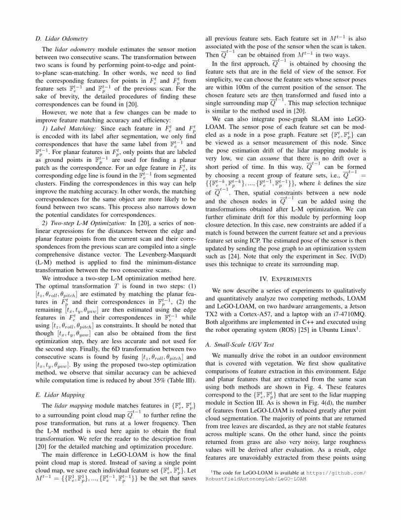
Fig. 3: Two-step optimization for the lidar odometry module.[tz, θroll, θpitch] is first obtained by matching the planar featuresextracted from ground points. [tx, ty, θyaw] are then estimated usingthe edge features extracted from segmented points while applying[tz, θroll, θpitch] as constraints.

three properties for each point: (1) its label as a ground pointor segmented point, (2) its column and row index in therange image, and (3) its range value. These properties willbe utilized in the following modules.

C. Feature Extraction

The feature extraction process is similar to the methodused in [20]. However, instead of extracting features fromraw point clouds, we extract features from ground points andsegmented points. Let S be the set of continuous points ofpi from the same row of the range image. Half of the pointsin S are on either side of pi. In this paper, we set |S| to 10.Using the range values computed during segmentation, wecan evaluate the roughness of point pi in S,

c =1

|S| · ‖ri‖‖ Σ

j∈S,j 6=i(rj − ri)‖. (1)

To evenly extract features from all directions, we dividethe range image horizontally into several equal sub-images.Then we sort the points in each row of the sub-image basedon their roughness values c. Similar to LOAM, we use athreshold cth to distinguish different types of features. Wecall the points with c larger than cth edge features, and thepoints with c smaller than cth planar features. Then nFe

edgefeature points with the maximum c, which do not belong tothe ground, are selected from each row in the sub-image.nFp

planar feature points with the minimum c, which maybe labeled as either ground or segmented points, are selectedin the same way. Let Fe and Fp be the set of all edgeand planar features from all sub-images. These features arevisualized in Fig. 2(d). We then extract nFe

edge featureswith the maximum c, which do not belong to the ground,from each row in the sub-image. Similarly, we extract nFp

planar features with the minimum c, which must be groundpoints, from each row in the sub-image. Let Fe and Fp be theset of all edge and planar features from this process. Here,we have Fe ⊂ Fe and Fp ⊂ Fp. Features in Fe and Fp areshown in Fig. 2(c). In this paper, we divide the 360◦ rangeimage into 6 sub-images. Each sub-image has a resolutionof 300 by 16. nFe , nFp , nFe and nFp are chosen to be 2, 4,40 and 80 respectively.

D. Lidar Odometry

The lidar odometry module estimates the sensor motionbetween two consecutive scans. The transformation betweentwo scans is found by performing point-to-edge and point-to-plane scan-matching. In other words, we need to findthe corresponding features for points in F t

e and F tp from

feature sets Ft−1e and Ft−1

p of the previous scan. For thesake of brevity, the detailed procedures of finding thesecorrespondences can be found in [20].

However, we note that a few changes can be made toimprove feature matching accuracy and efficiency:

1) Label Matching: Since each feature in F te and F t

p

is encoded with its label after segmentation, we only findcorrespondences that have the same label from Ft−1

e andFt−1p . For planar features in F t

p , only points that are labeledas ground points in Ft−1

p are used for finding a planarpatch as the correspondence. For an edge feature in F t

e , itscorresponding edge line is found in the Ft−1

e from segmentedclusters. Finding the correspondences in this way can helpimprove the matching accuracy. In other words, the matchingcorrespondences for the same object are more likely to befound between two scans. This process also narrows downthe potential candidates for correspondences.

2) Two-step L-M Optimization: In [20], a series of non-linear expressions for the distances between the edge andplanar feature points from the current scan and their corre-spondences from the previous scan are compiled into a singlecomprehensive distance vector. The Levenberg-Marquardt(L-M) method is applied to find the minimum-distancetransformation between the two consecutive scans.

We introduce a two-step L-M optimization method here.The optimal transformation T is found in two steps: (1)[tz, θroll, θpitch] are estimated by matching the planar fea-tures in F t

p and their correspondences in Ft−1p , (2) the

remaining [tx, ty, θyaw] are then estimated using the edgefeatures in F t

e and their correspondences in Ft−1e while

using [tz, θroll, θpitch] as constraints. It should be noted thatthough [tx, ty, θyaw] can also be obtained from the firstoptimization step, they are less accurate and not used forthe second step. Finally, the 6D transformation between twoconsecutive scans is found by fusing [tz, θroll, θpitch] and[tx, ty, θyaw]. By using the proposed two-step optimizationmethod, we observe that similar accuracy can be achievedwhile computation time is reduced by about 35% (Table III).

E. Lidar Mapping

The lidar mapping module matches features in {Fte, Ft

p}to a surrounding point cloud map Q

t−1to further refine the

pose transformation, but runs at a lower frequency. Thenthe L-M method is used here again to obtain the finaltransformation. We refer the reader to the description from[20] for the detailed matching and optimization procedure.

The main difference in LeGO-LOAM is how the finalpoint cloud map is stored. Instead of saving a single pointcloud map, we save each individual feature set {Ft

e, Ftp}. Let

M t−1 = {{F1e,F1

p}, ..., {Ft−1e ,Ft−1

p }} be the set that saves

all previous feature sets. Each feature set in M t−1 is alsoassociated with the pose of the sensor when the scan is taken.Then Q

t−1can be obtained from M t−1 in two ways.

In the first approach, Qt−1

is obtained by choosing thefeature sets that are in the field of view of the sensor. Forsimplicity, we can choose the feature sets whose sensor posesare within 100m of the current position of the sensor. Thechosen feature sets are then transformed and fused into asingle surrounding map Q

t−1. This map selection technique

is similar to the method used in [20].We can also integrate pose-graph SLAM into LeGO-

LOAM. The sensor pose of each feature set can be mod-eled as a node in a pose graph. Feature set {Ft

e,Ftp} can

be viewed as a sensor measurement of this node. Sincethe pose estimation drift of the lidar mapping module isvery low, we can assume that there is no drift over ashort period of time. In this way, Q

t−1can be formed

by choosing a recent group of feature sets, i.e., Qt−1

={{Ft−k

e ,Ft−kp }, ..., {Ft−1

e ,Ft−1p }}, where k defines the size

of Qt−1

. Then, spatial constraints between a new nodeand the chosen nodes in Q

t−1can be added using the

transformations obtained after L-M optimization. We canfurther eliminate drift for this module by performing loopclosure detection. In this case, new constraints are added if amatch is found between the current feature set and a previousfeature set using ICP. The estimated pose of the sensor is thenupdated by sending the pose graph to an optimization systemsuch as [24]. Note that only the experiment in Sec. IV(D)uses this technique to create its surrounding map.

IV. EXPERIMENTS

We now describe a series of experiments to qualitativelyand quantitatively analyze two competing methods, LOAMand LeGO-LOAM, on two hardware arrangements, a JetsonTX2 with a Cortex-A57, and a laptop with an i7-4710MQ.Both algorithms are implemented in C++ and executed usingthe robot operating system (ROS) [25] in Ubuntu Linux1.

A. Small-Scale UGV Test

We manually drive the robot in an outdoor environmentthat is covered with vegetation. We first show qualitativecomparisons of feature extraction in this environment. Edgeand planar features that are extracted from the same scanusing both methods are shown in Fig. 4. These featurescorrespond to the {Ft

e,Ftp} that are sent to the lidar mapping

module in Section III. As is shown in Fig. 4(d), the numberof features from LeGO-LOAM is reduced greatly after pointcloud segmentation. The majority of points that are returnedfrom tree leaves are discarded, as they are not stable featuresacross multiple scans. On the other hand, since the pointsreturned from grass are also very noisy, large roughnessvalues will be derived after evaluation. As a result, edgefeatures are unavoidably extracted from these points using

1The code for LeGO-LOAM is available at https://github.com/RobustFieldAutonomyLab/LeGO-LOAM

Fig. 4: Edge and planar features obtained from two different lidarodometry and mapping frameworks in an outdoor environmentcovered by vegetation. Edge and planar features are colored greenand pink, respectively. The features obtained from LOAM areshown in (b) and (c). The features obtained from LeGO-LOAMare shown in (d) and (e). Label (i) indicates a tree, (ii) indicates astone wall, and (iii) indicates the robot.

(a) LOAM (b) LeGO-LOAM

Fig. 5: Maps from both LOAM and LeGO-LOAM over the terrainshown in Fig. 4(a). The trees marked by white arrows in (a)represent the same tree.

the original LOAM. As is shown in Fig. 4(c), edge featuresthat are extracted from the ground are often unreliable.

Though we can change the roughness threshold cth forextracting edge and planar features in LOAM to reduce thenumber of features and filter out unstable features from grassand leaves, we encounter worse results after applying suchchanges. For example, we can increase cth to extract morestable edge features from an environment, but this changemay result in an insufficient number of useful edge featuresif the robot enters a relatively clean environment. Similarly,decreasing cth will also give rise to a lack of useful planarfeatures when the robot moves from a clean environment toa noisy environment. Throughout all experiments here, weuse the same cth for both LOAM and LeGO-LOAM.

Now we compare the mapping results from both methodsover the test environment. To mimic a challenging potentialUGV operational scenario, we perform a series of aggressiveyaw maneuvers. Note that both methods are fed an identicalinitial translational and rotational guess, which is obtainedfrom an IMU, throughout all experiments in the paper. Theresulting point cloud map after 60 seconds of operation is

TABLE I: Large-Scale Outdoor Datasets

Experiment ScanNumber

ElevationChange (m)

TrajectoryLength (km)

1 8077 11 1.092 8946 11 1.243 20834 19 2.71

shown in Fig. 5. Due to erroneous feature associations causedby unstable features, the map from LOAM diverges twiceduring operation. The three tree trunks that are highlighted bywhite arrows in Fig. 5(a) represent the same tree in reality. Avisualization of the full mapping process for both odometrymethods can be found in the video attachment2.

B. Large-Scale UGV Tests

We next perform quantitative comparisons of LOAM andLeGO-LOAM over three large-scale datasets, which will bereferred to as experiments 1, 2 and 3. The first two werecollected on the Stevens Institute of Technology campus,with numerous buildings, trees, roads and sidewalks. Theseexperiments and their environment are illustrated in Fig. 6(a).Experiment 3 spans a forested hiking trail, which featurestrees, asphalt roads and trail paths covered by grass and soil.The environment in which experiment 3 was performed isshown in Fig. 8. The details of each experiment are listed inTable I. To perform a fair comparison, all of the performanceand accuracy results shown for each experiment are averagedover 10 trials of real-time playback of each dataset.

1) Experiment 1: The first experiment is designed toshow that both LOAM and LeGO-LOAM can achieve low-drift pose estimation in an urban environment with smoothmotion. We avoid aggressive yaw maneuvers, and we avoiddriving the robot through sparse areas where only a fewstable features can be acquired. The robot is operated onsmooth roads during the whole data logging process. Theinitial position of the robot, which is marked in Fig. 6(b), ison a slope. The robot returns to the same position after 807seconds of travel with an average speed of 1.35m/s.

To evaluate the pose estimation accuracy of both meth-ods, we compare the translational and rotational differencebetween the final pose and the initial pose. Here, the initialpose is defined as [0, 0, 0, 0, 0, 0] through all experiments. Asis shown in Table V, both LOAM and LeGO-LOAM achievesimilar low-drift pose estimation over two different hardwarearrangements. The final map from LeGO-LOAM, when runon a Jetson, is shown in Fig. 6(b).

2) Experiment 2: Though experiment 2 is carried outin the same environment as experiment 1, its trajectory isslightly different, driving across a sidewalk that is shownin Fig. 7(a). This sidewalk represents an environment whereLOAM may often fail. A wall and pillars are on one endof the sidewalk - the edge and planar features that areextracted from these structures are stable. The other end ofthe sidewalk is an open area covered with noisy objects,i.e., grass and trees, which will result in unreliable featureextraction. As a result, LOAM’s pose estimation diverges

2https://youtu.be/O3tz_ftHV48

(a) Satellite image (b) Experiment 1 (c) Experiment 2

Fig. 6: LeGO-LOAM maps from experiments 1 and 2. The color variation in (c) indicates true elevation change. Since the robot’s initialposition in experiment 1 is on a slope, the color variation in (b) does not represent true elevation change.

(a) Satellite image (b) LOAM (c) LeGO-LOAM (d) LOAM (e) LeGO-LOAM

Fig. 7: A scenario where LOAM fails over a sidewalk crossing the Stevens campus in experiment 2 (the leftmost sidewalk in image (a)above). One end of the sidewalk is supported by features from a nearby building. The other end of the sidewalk is surrounded primarilyby noisy objects, i.e., grass and trees. Without point cloud segmentation, unreliable edge and planar features will be extracted from suchobjects. Images (b) and (d) show that LOAM fails after passing over the sidewalk.

Fig. 8: Experiment 3 LeGO-LOAM mapping result.

after driving over this sidewalk (Fig. 7(b) and (d)). LeGO-LOAM has no such problem as: 1) no edge features areextracted from ground that is covered by grass, and 2)noisy sensor readings from tree leaves are filtered out aftersegmentation. An accuracy comparison of both methods isshown in Table V. In this experiment, LeGO-LOAM achieveshigher accuracy than LOAM by an order of magnitude.

3) Experiment 3: The dataset for experiment 3 was loggedfrom a forested hiking trail, where the UGV was driven atan average speed of 1.3m/s. The robot returns to the initialposition after 35 minutes of driving. The elevation change inthis environment is about 19 meters. The UGV is driven onthree road surfaces: dirt-covered trails, asphalt, and ground

covered by grass. Representative images of such surfacessare shown respectively at bottom of Fig. 8. Trees or bushesare present on at least one side of the road at all times.

We first test LOAM’s accuracy in this environment.The resulting maps diverge at various locations on bothcomputers used. The final translational and rotational errorwith respect to the UGV’s initial position are 69.40m and27.38◦ on the Jetson, and 62.11m and 8.50◦ on the laptop.The resulting trajectories from 10 trials on both hardwarearrangements are shown in Fig. 9(a) and (b).

When LeGO-LOAM is applied to this dataset, the finalrelative translational and rotational errors are 13.93m and7.73◦ on the Jetson, and 14.87m and 7.96◦ on the laptop.The final point cloud map from LeGO-LOAM on the Jetsonis shown in Fig. 8 overlaid atop a satellite image. A localmap, which is enlarged at the center of Fig. 8, shows that thepoint cloud map from LeGO-LOAM matches well with threetrees visible in the open. High consistency is shown amongall paths obtained from LeGO-LOAM on both computers.Fig. 9(c) and (d) show ten trials run on each computer.

C. Benchmarking Results

1) Feature number comparison: We show a comparisonof feature extraction across both methods in Table II. Thefeature content of each scan is averaged over 10 trials foreach dataset. After point cloud segmentation, the numberof features that need to be processed by LeGO-LOAM isreduced by at least 29%, 40%, 68% and 72% for sets Fe,Fp, Fe and Fp respectively.

(a) LOAM on Jetson (b) LOAM on laptop

(c) LeGO-LOAM on Jetson (d) LeGO-LOAM on laptop

Fig. 9: Paths produced by LOAM and LeGO-LOAM across 10trials, and 2 computers, with the experiment 3 dataset.

TABLE II: Average feature content of a scan after feature extraction

Scen

ario Edge

Features Fe

PlanarFeatures Fp

EdgeFeatures Fe

PlanarFeatures Fp

LOAM LeGO-LOAM LOAM LeGO-

LOAM LOAM LeGO-LOAM LOAM LeGO-

LOAM

1 157 102 323 152 878 253 4849 13192 145 102 331 154 798 254 4677 12273 174 101 172 103 819 163 6056 1146

2) Iteration number comparison: The results of applyingthe proposed two-step L-M optimization method are shownin Table III. We first apply the original L-M optimizationwith LeGO-LOAM, which means that we minimize thedistance function obtained from edge and planar featurestogether. Then we apply the two-step L-M optimization forLeGO-LOAM: 1) planar features in Fp are used to obtain[tz, θroll, θpitch] and 2) edge features in Fe are used to obtain[tx, ty, θyaw]. The average iteration number when the L-Mmethod terminates after processing one scan is logged forcomparison. When two-step optimization is used, the step-1optimization is finished in 2 iterations in experiments 1 and2. Though the iteration count of the step-2 optimization issimilar to the quantity of the original L-M method, fewerfeatures are processed. As a result, the runtime for lidarodometry is reduced by 34% to 48% after using two-stepL-M optimization. The runtime for two-step optimization isshown in Table IV.

3) Runtime comparison: The runtime for each module ofLOAM and LeGO-LOAM over two computers is shown inTable IV. Using the proposed framework, the runtime of thefeature extraction and lidar odometry modules are reducedby one order of magnitude in LeGO-LOAM. Note that theruntime of these two modules in LOAM is more than 100mson a Jetson. As a result, many scans are skipped because real-time performance is not achieved by LOAM on an embeddedsystem. The runtime of lidar mapping is also reduced by atleast 60% when LeGO-LOAM is used.

4) Pose error comparison: By setting the initial pose to[0, 0, 0, 0, 0, 0] in all experiments, we compute the relativepose estimation error by comparing the final pose with the

TABLE III: Iteration number comparison for LeGO-LOAM

Scenario Original Opt. Two-step Opt.Iter. Num. Time Step 1

Iter. NumStep 2

Iter. Num

Jets

on 1 16.6 34.5 1.9 17.52 15.7 32.9 1.7 16.73 20.0 27.7 4.7 18.9

i7

1 17.3 13.1 1.8 18.22 16.5 12.3 1.6 17.53 20.5 10.4 4.7 19.8

TABLE IV: Runtime of modules for processing one scan (ms)

Scenario Segmentation Extraction Odometry MappingLOAM LeGO-

LOAM LOAM LeGO-LOAM LOAM LeGO-

LOAM LOAM LeGO-LOAM

Jets

on 1 N/A 29.3 105.1 9.1 133.4 19.3 702.3 266.72 N/A 29.9 106.7 9.9 124.5 18.6 793.6 278.23 N/A 36.8 104.6 6.1 122.1 18.1 850.9 253.3

i7

1 N/A 16.7 50.4 4.0 69.8 6.8 289.4 108.22 N/A 17.0 49.3 4.4 66.5 6.5 330.5 116.73 N/A 20.0 48.5 2.3 63.0 6.1 344.9 101.7

initial pose. Rotational error (in degrees) and translationalerror (in meters) are listed in Table V for both methods overboth computers. By using the proposed framework, LeGO-LOAM can achieve comparable or better position estimationaccuracy with less computation time.

D. Loop Closure Test using KITTI Dataset

Our final experiment applies LeGO-LOAM to the KITTIdataset [21]. Since the tests of LOAM over the KITTIdatasets in [20] run at 10% of the real-time speed, weonly explore LeGO-LOAM and its potential for real-timeapplications with embedded systems, where the length oftravel is significant enough to require a full SLAM solution.The results from LeGO-LOAM on a Jetson using sequence00 are shown in Fig. 10. To achieve real-time performanceon the Jetson, we downsample the scan from the HDL-64Eto the same range image that is used in Section III for theVLP-16. In other words, 75% of the points of each scanare omitted before processing. ICP is used here for addingconstraints between nodes in the pose graph. The graphis then optimized using iSAM2 [24]. At last, we use theoptimized graph to correct the sensor pose and map. Moreloop closure tests can be found in the video attachment.

V. CONCLUSIONS AND DISCUSSION

We have proposed LeGO-LOAM, a lightweight andground-optimized lidar odometry and mapping method, forperforming real-time pose estimation of UGVs in complexenvironments. LeGO-LOAM is lightweight, as it can be usedon an embedded system and achieve real-time performance.LeGO-LOAM is also ground-optimized, leveraging groundseparation, point cloud segmentation, and improved L-Moptimization. Valueless points that may represent unreliablefeatures are filtered out in this process. The two-step L-Moptimization computes different components of a pose trans-formation separately. The proposed method is evaluated ona series of UGV datasets gathered in outdoor environments.The results show that LeGO-LOAM can achieve similaror better accuracy when compared with the state-of-the-art

TABLE V: Relative pose estimation error when returning to start

Scenario Method Roll Pitch Yaw TotalRot.(◦) X Y Z Total

Trans.(m)

Jets

on

1 LOAM 1.16 2.63 2.5 3.81 1.33 2.91 0.43 3.23LeGO-LOAM 0.46 0.91 1.98 2.23 0.12 0.07 1.26 1.27

2 LOAM 7.05 5.06 9.4 12.80 7.71 6.31 4.32 10.86LeGO-LOAM 0.61 0.70 0.32 0.99 0.04 0.10 0.34 0.36

3 LOAM 7.55 3.20 26.12 27.38 34.61 56.19 21.46 69.40LeGO-LOAM 4.62 5.45 2.95 7.73 5.35 7.95 10.11 13.93

i7

1 LOAM 0.28 1.98 1.74 2.65 0.39 0.03 0.21 0.44LeGO-LOAM 0.33 0.17 2.06 2.09 0.03 0.02 0.22 0.22

2 LOAM 21.49 4.86 4.34 22.46 1.39 2.59 11.63 11.99LeGO-LOAM 0.18 0.85 0.64 1.08 0.04 0.12 0.04 0.14

3 LOAM 6.27 3.08 4.83 8.50 16.84 58.81 10.74 62.11LeGO-LOAM 4.57 5.39 3.68 7.96 6.69 7.79 10.76 14.87

(a) (b)

Fig. 10: LeGO-LOAM, KITTI dataset loop closure test, using theJetson. Color variation indicates elevation change.

algorithm LOAM. The computation time of LeGO-LOAMis also greatly reduced. Future work involves exploring itsapplication to other classes of vehicles.

Though LeGO-LOAM is especially optimized for pose es-timation on ground vehicles, its application could potentiallybe extended to other vehicles, e.g., unmanned aerial vehicles(UAVs), with minor changes. When applying LeGO-LOAMto a UAV, we would not assume the ground is present ina scan. A scan’s point cloud would be segmented withoutground extraction. The feature extraction process would bethe same for the selection of Fe, Fe and Fp. Instead ofextracting planar features for Fp from points that are labeledas ground points, the features in Fp would be selected fromall segmented points. Then the original L-M method wouldbe used to obtain the transformation between two scansinstead of using the two-step optimization method. Thoughthe computation time will increase after these changes,LeGO-LOAM is still efficient, as a large number of points areomitted in noisy outdoor environments after segmentation.The accuracy of the estimated feature correspondences mayimprove, as they benefit from segmentation. In addition, theability to perform loop closures with LeGO-LOAM onlinemakes it a useful tool for long-duration navigation tasks.

REFERENCES

[1] P.J. Besl and N.D. McKay, “A Method for Registration of 3D Shapes,”IEEE Transactions on Pattern Analysis and Machine Intelligence, vol.14(2): 239-256, 1992.

[2] S. Rusinkiewicz and M. Levoy, “Efficient Variants of the ICP Al-gorithm,” Proceedings of the Third International Conference on 3-DDigital Imaging and Modeling, pp. 145-152, 2001.

[3] Y. Chen and G. Medioni, “Object Modelling by Registration ofMultiple Range Images,” Image and Vision Computing, vol. 10(3):145-155, 1992.

[4] A. Segal, D. Haehnel, and S. Thrun, “Generalized-ICP,” Proceedingsof Robotics: Science and Systems, 2009.

[5] R.A. Newcombe, S. Izadi, O. Hilliges, D. Molyneaux, D. Kim, A.J.Davison, P. Kohi, J. Shotton, S. Hodges, and A. Fitzgibbon, “KinectFu-sion: Real-time Dense Surface Mapping and Tracking,” Proceedings ofthe IEEE International Symposium on Mixed and Augmented Reality,pp. 127-136, 2011.

[6] A. Nuchter, “Parallelization of Scan Matching for Robotic 3D Map-ping,” Proceedings of the 3rd European Conference on Mobile Robots,2007.

[7] D. Qiu, S. May, and A. Nuchter, “GPU-Accelerated Nearest NeighborSearch for 3D Registration,” Proceedings of the International Confer-ence on Computer Vision Systems, pp. 194-203, 2009.

[8] D. Neumann, F. Lugauer, S. Bauer, J. Wasza, and J. Hornegger, “Real-time RGB-D Mapping and 3D Modeling on the GPU Using theRandom Ball Cover Data Structure,” IEEE International Conferenceon Computer Vision Workshops, pp. 1161-1167, 2011.

[9] R.B. Rusu, Z.C. Marton, N. Blodow, and M. Beetz, “Learning In-formative Point Classes for the Acquisition of Object Model Maps,”Proceedings of the IEEE International Conference on Control, Au-tomation, Robotics and Vision, pp. 643-650, 2008.

[10] R.B. Rusu, G. Bradski, R. Thibaux, and J. Hsu, “Fast 3D Recognitionand Pose Using the Viewpoint Feature Histogram,” Proceedings of theIEEE/RSJ International Conference on Intelligent Robots and Systems,pp. 2155-2162, 2010.

[11] Y. Li and E.B. Olson, “Structure Tensors for General Purpose LIDARFeature Extraction,” Proceedings of the IEEE International Conferenceon Robotics and Automation, pp. 1869-1874, 2011.

[12] J. Serafin, E. Olson, and G. Grisetti, “Fast and Robust 3D FeatureExtraction from Sparse Point Clouds,” Proceedings of the IEEE/RSJInternational Conference on Intelligent Robots and Systems, pp. 4105-4112, 2016.

[13] M. Bosse and R. Zlot, “Keypoint Design and Evaluation for PlaceRecognition in 2D Lidar Maps,” Robotics and Autonomous Systems,vol. 57(12): 1211-1224, 2009.

[14] R. Zlot and M. Bosse, “Efficient Large-scale 3D Mobile Mapping andSurface Reconstruction of an Underground Mine,” Proceedings of the8th International Conference on Field and Service Robotics, 2012.

[15] B. Steder, G. Grisetti, and W. Burgard, ”Robust Place Recognition for3D Range Data Based on Point Features,” Proceedings of the IEEEInternational Conference on Robotics and Automation, pp. 1400-1405,2010.

[16] W.S. Grant, R.C. Voorhies, and L. Itti, “Finding Planes in LiDARPoint Clouds for Real-time Registration,” Proceedings of the IEEE/RSJInternational Conference on Intelligent Robots and Systems, pp. 4347-4354, 2013.

[17] M. Velas, M. Spanel, and A. Herout, “Collar Line Segments for FastOdometry Estimation from Velodyne Point Clouds,” Proceedings ofthe IEEE International Conference on Robotics and Automation, pp.4486-4495, 2016.

[18] R. Dube, D. Dugas, E. Stumm, J. Nieto, R. Siegwart, and C. Cadena,”SegMatch: Segment Based Place Recognition in 3D Point Clouds,”Proceedings of the IEEE International Conference on Robotics andAutomation, pp. 5266-5272, 2017.

[19] J. Zhang and S. Singh, “LOAM: Lidar Odometry and Mapping inReal-time,” Proceedings of Robotics: Science and Systems, 2014.

[20] J. Zhang and S. Singh, “Low-drift and Real-time Lidar Odometry andMapping,” Autonomous Robots, vol. 41(2): 401-416, 2017.

[21] A. Geiger, P. Lenz, and R. Urtasun, “Are We Ready for AutonomousDriving? The KITTI Vision Benchmark Suite”, Proceedings of theIEEE International Conference on Computer Vision and PatternRecognition, pp. 3354-3361, 2012.

[22] M. Himmelsbach, F.V. Hundelshausen, and H-J. Wuensche, “FastSegmentation of 3D Point Clouds for Ground Vehicles,” Proceedingsof the IEEE Intelligent Vehicles Symposium, pp. 560-565, 2010.

[23] I. Bogoslavskyi and C. Stachniss, “Fast Range Image-based Segmen-tation of Sparse 3D Laser Scans for Online Operation,” Proceedingsof the IEEE/RSJ International Conference on Intelligent Robots andSystems, pp. 163-169, 2016.

[24] M. Kaess, H. Johannsson, R. Roberts, V. Ila, J.J. Leonard, and F.Dellaert, “iSAM2: Incremental Smoothing and Mapping Using theBayes Tree,” The International Journal of Robotics Research 31, vol.31(2): 216-235, 2012.

[25] M. Quigley, K. Conley, B. Gerkey, J. Faust, T. Foote, J. Leibs,R. Wheeler, and A.Y. Ng, “ROS: An Open-source Robot OperatingSystem,” IEEE ICRA Workshop on Open Source Software, 2009.