Barcelona Graduate School of Economics

Final Master Project

Legislative Quota, Women Empowermentand Development: Evidence from Tanzania

Authors:

Gregory Raiffa

Ericka Sánchez

Jan Stübner

Feodora Teti

Andreas Wohlhüter

Abstract

This paper analyzes whether the legislative women’s quota implemented in Tanzania has

helped to reduce the existing gender gap in that country. We focus on a set of development

indicators indicated by the literature and an analysis of female political activity. We exploit

the variation in the number of female representatives across the 131 districts of Tanzania,

employing a Difference and Differences approach including fixed effects and controlling for a

number of socioeconomic variables. Our analysis indicates that the legislative women’s quota in

Tanzania has led to significant reductions in the gender gap and improvements for women. The

quota has effectively increased political participation in accordance with its goals, and the level

of female representation continues to rise. We find evidence that the quota has reduced the

gender gap in education for certain age groups, and we find indications of small improvements

to female empowerment. In accordance with previous findings in other countries, we find that

the increased female representation has led to substantial investments in water infrastructure

that has greatly increased the number of people with access to clean water. While we do not

find significant health impacts, this may be due to limitations in our dataset.

June 5th, 2015

1 Introduction

The improvement of global gender equality and the empowerment of women worldwide is one

of the eight UN millennium development goals. In the past two decades significant progress has

been made in achieving this goal. According to the world gender gap report in 2014, the gender

gaps in women’s educational attainment (94%) and in health and survival (96%) have almost

been closed 1. In contrast, the gender inequality in economic participation and opportunity (60%),

and in particular the gender gap in political empowerment (21%) remain far from being balanced

Hausmann et al. (2014).

Although there has been great progress in some areas, gender inequality is still prominent

in many societal aspects, particularly in the developing world. Women are often not granted the

same rights and opportunities as men and are left with social and economic disadvantages, which

have negative effects for an economy as a whole. Since human capital is one of the main drivers of

an economy, the underuse of half of a country’s population can have far-reaching consequences for

long-term economic growth and development.

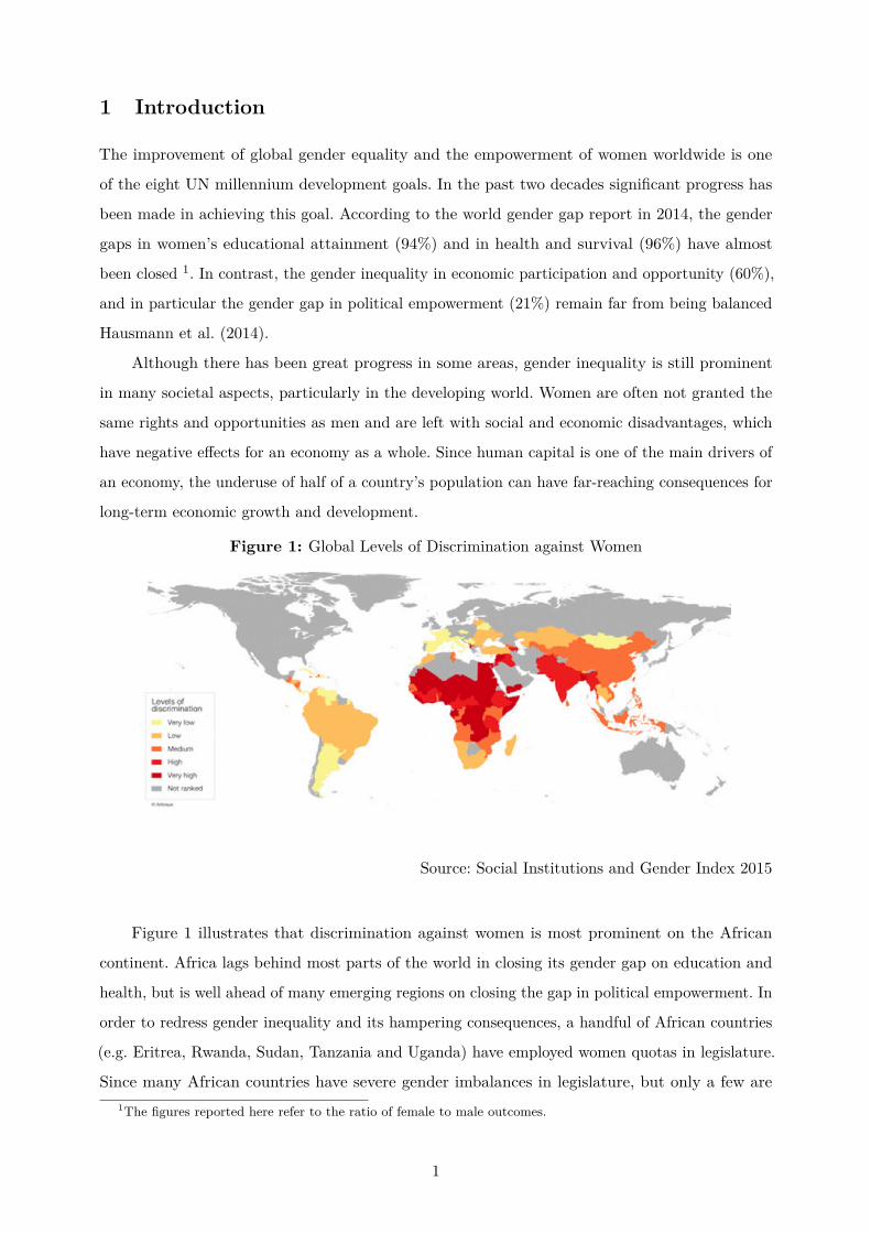
Figure 1: Global Levels of Discrimination against Women

Source: Social Institutions and Gender Index 2015

Figure 1 illustrates that discrimination against women is most prominent on the African

continent. Africa lags behind most parts of the world in closing its gender gap on education and

health, but is well ahead of many emerging regions on closing the gap in political empowerment. In

order to redress gender inequality and its hampering consequences, a handful of African countries

(e.g. Eritrea, Rwanda, Sudan, Tanzania and Uganda) have employed women quotas in legislature.

Since many African countries have severe gender imbalances in legislature, but only a few are1The figures reported here refer to the ratio of female to male outcomes.

1

employing a quota system to address this disparity, it is crucial to evaluate the impact of such a

policy in order to evaluate its usefulness for other developing countries.

In this paper we focus on the special seat system for women in Tanzania. Our main objective

is to analyze the effects of this quota system on a set of development indicators and by these means

to provide a sophisticated answer to the following policy question: Did the legislative women’s

quota reduce the existing gender gap in Tanzania? In particular, we are interested in outcomes

related to education, health, the quality of infrastructure and female empowerment.

Tanzania’s quota system was first introduced with relatively mild requirements in 1985,

though the requirements were increased substantially for the 1995 elections to require female

representation to account for at least 15% of traditional seats in parliament. This requirement

was increased to 20% in 2000 and to 30% in 2005. Tanzania is a particularly interesting case

to study for a number of reasons. Firstly, the prevailing patriarchal society, favoring segregate

gender roles, makes it a good starting point to analyze the effect of the legislative women’s quota.

Furthermore, after the special seat system for women was first introduced, women managed to

push for laws that address women’s concerns in several areas, such as maternity leave for mothers,

a sexual offence bill, a law that promotes enrollment of women in tertiary education and a land

law reform that addresses discriminatory practices against women (Meena (2003)). Furthermore,

while data availability is typically a major issue for developing countries, data for Tanzania is

readily available.

Besides the direct channel of more female-oriented policies, the quota might also induce an

indirect change in women’s roles in society, i.e. a higher representation of women in politically

influential positions might incentivize young women to pursue similar paths and at the same

time lead to changes in cultural norms. However, the effectiveness of a legislative gender quota is

debatable. Duflo (2012) concludes that a one-time impulsion of women’s rights is not sufficient

in order to change entrenched political norms and values that discriminate against women, but

instead further complementing measures are required.

In order to measure these effects we exploit the variation in the number of female MPs across

the 131 districts of Tanzania employing a Difference -in- Differences (DiD) approach including

fixed effects and controlling for a number of socioeconomic variables. For this purpose we are

using various data sources. We are working with four extensive micro level datasets (Demographic

and Health Surveys (DHS) with more than 178,000 observations), ranging from 2003 to 2012

and a self-generated database, which contains information about Tanzanian MPs for the past

three legislative terms (2000, 2005, 2010). Using GPS data we match villages from the micro-level

dataset with the districts of the country and the information on female representation by district.

We find significant evidence that the quota has reduced the gender gap in education for certain age

2

groups, moreover we find indications of small improvements for female empowerment for some age

groups. In accordance with previous findings in other countries, we find that an increase in female

representation leads to substantial investments in water infrastructure that greatly increased the

number of people with access to clean water. While we do not find significant health impacts, this

may be due to limitations in our dataset.

The rest of this paper is structured as follows. Section 2 provides a literature review. Section

3 gives an overview of the quota in Tanzania, its implementation and its effect on female political

participation. Section 4 looks at testable implications. Section 5 describes our empirical strategy

and Section 6 describes our dataset in more detail. Section 7 provides our main analysis and

section 8 provides our policy evaluation.

2 Literature Review

There is substantial research that analyzes the relationship between gender inequality and economic

growth and development. The theoretical literature regarding gender inequality in education focuses

on the insufficient exploitation of human capital. Klasen (2002) argues that a higher marginal

return to education exists for girls, that if exploited could lead to substantial growth. Furthermore,

higher education of women is expected to lead to both lower fertility and child mortality rates

as well as a better educated following generation (Esteve-Volart (2004) ; Cavalcanti and Tavares

(2007)).

The same argument is often applied when considering the effect of gender gaps in labor

market participation on economic growth, i.e. that existing human capital is not being efficiently

exploited (Klasen (2002)). Moreover, higher female employment has been shown to increase

women’s bargaining power at home, which consequently might lead to higher investments in

children’s health and education, fostering human capital formation of the following generation

(Seguino and Floro (2003)). Finally, recent literature has argued that women tend to be less

prone to corruption than men (Dollar et al. (2001), Swamy et al. (2000)). Hence, a higher female

participation in the labor force and higher education for women may lead to less corrupt governance

in business and policymaking.

Another line of research has demonstrated that increasing female political participation can

reduce the gender gap in a variety of areas. Thomas (1991) as well as Besley and Case (2003) find

evidence that increased political representation of women is correlated with different spending

priorities, and Clots-Figueroa (2011) leverages close elections between men and women in India

to show that women tend to invest more in education and make more pro-female policies. Aside

from the direct effect of passing more female-oriented policies, there is increasing evidence that

3

increased female representation can reduce the gender gap through its effect on social norms.

Beaman et al. (2012) demonstrate that female leadership has an impact on adolescent girls’ career

aspirations and educational attainments, which they attribute to a role-model effect. According

to them, this role-model effect may influence girls’ notion of women’s status in society and thus

may influence them to break with prevalent gender stereotypes. Therefore, being exposed to a

female leader might increase girls’ ambitions and their propensity to enter male dominated areas.

For rural India, the gender gap in aspirations closed by 25% for parents and by 32% for youths

in villages that had exposure to a female leader for two election periods. Furthermore, in these

villages the gender gap in educational attainment was eradicated and girls tended to spend less

time on household work Beaman et al. (2012).

Recent literature has demonstrated that women quotas lead to increases in women participation

in government. Yoon (2011) gives evidence that women quotas in Africa increase female legislative

representation, and Jones (1998) finds similar evidence for Argentina. Dahlerup (2003) also

documents the cases of Rwanda, South Africa and Costa Rica, where gender quotas have led to

large increases of women representation in government.

Evidence on such quotas from a variety of settings indicates that required political represen-

tation has an effect on policy choices and outcomes. Chattopadhyay and Duflo (2004) study a

reservation policy for women in rural India. They find that gender-specific preferences of political

leaders have significant effects on policy choices, implying that female political leaders better

represent women’s preferences. In regions where women complained relatively more about specific

types of infrastructure, women-led councils showed higher public spending for these types of infras-

tructure. Beaman et al. (2010) use data from the Millennial Survey spanning eleven Indian states

and show that on average, gender quotas result in increased investment in water infrastructure

and education. Pande (2003), when looking instead at required political participation for various

caste groups in India, finds increased transfers to those groups. On the other hand, Kotsadam and

Mans investigate the effects of gender quotas in national elections in Latin America and find that

while quotas substantially increased the number of women in parliament, they had no effect on

political participation, public policy, or corruption.

Multiple studies demonstrate a change in cultural norms following the introduction of women

quotas. Beaman et al. (2009) present evidence for changes in voter attitudes after being exposed

to the quotas. According to their results, women were more likely to campaign and get elected

conventionally in councils that were required to have a female leader in the previous two elections.

Furthermore, reservation led to a decrease in gender discrimination by men. Beaman et al. (2010)

further show that the likelihood that a woman speaks at a village meeting in India increases by

25% when local political leader positions are reserved for women. Furthermore, there is evidence

4

that the effects of women’s quotas persist over time. Paola et al. (2015) show that gender quotas

in Italy increase women’s representation in politics even after the quota was terminated. To our

best knowledge, we are the first to quantitatively analyze the effects of the legislative women’s

quota in Tanzania.

3 Quota in Tanzania

In order to better understand the effects of the quota system in Tanzania and to guide our

micro-level analysis of outcomes, we first investigate the direct effects of the quota on female

political participation in Tanzania. We use a three phase analysis consisting of 1) identifying the

quota framework 2) evaluating the implementation of the quota and 3) analysing the political

activity of female MPs.

3.1 Quota Framework

The quota in Tanzania was implemented to address large gender gaps in parliamentary represen-

tation. High female participation in the struggle for independence and the nationalist movement

attracted women to politics and helped motivate the need to address the gender gap in repre-

sentation (Yoon (2008)). The quota is implemented through reserved seats called Special Seats.

The system was implemented in 1985, originally with 15 seats reserved for women. In 1995 the

quota increased to require that 15% (37 seats in 1995) of the total number of traditional seats in

parliament be added as special seats for women. In 2000 it was increased to 20%, and in 2005 it

was increased again to 30% (Meena (2003); Yoon (2008); Yoon (2011)). The total size of parliament

has been increasing over this timeline as well.

3.2 Implementation of the Quota

Table 1 shows the progression of the quota and female representation in parliament for the years

1985 to 2010. In each year the number of special seats women in parliament surpassed the level

mandated by the quota. Furthermore, female representation continued to increase in the 2010

elections despite no increase in the quota. We are also interested in how the number of women

elected to a constituency has changed over time. If the increased female representation resulting

from the quota has caused more women to feel capable of leadership, or if the increased female

representation has caused the public of Tanzania to have more faith in women as leaders, we might

expect to see more women winning constituency seats. Indeed we find that the number of women

elected to a constituency has also been increasing to keep track with the quota. These women

5

made up between 17% and 19% of all women in parliament for each of the elections between 1985

and 2010.

Table 1: Women in Parliament

Year Special seatsfor Women

ConstituencyWomen

TotalWomen

Total Seats inParliament

% Women Quota

1985 15 4 24 244 9.84% 15 seats1990 15 5 28 255 10.98% 15 seats1995 37 8 47 275 17.09% 15%2000 48 12 63 295 21.36% 20%2005 75 17 97 323 30.03% 30%2010 102 21 126 357 35.29% 30%

Source: Yoon (2008), Keith (2011)

3.3 Political Activity of Female MPs

Thus far we have established that the quota has successfully led to a corresponding increase in

female representation. In order to fully assess the impact of the quota, we next evaluate what these

additional women have done once they have reached parliament. Ideally we would analyze the

number and scale of policies put forth by female MPs compared to their male counterparts, as well

as the pass rate of such policies. Furthermore we would identify any systematic differences in the

type of policies put forth by men vs. women. Unfortunately we were unable to obtain data at this

level of detail. Instead, we are limited to data on the gender makeup of parliamentary committees

over the past four terms. Committees in Tanzania are made up of “[. . . ] several members of

parliament with a specific goal and time-frame regarding a particular/distinct subject of concern”

POLIS 2015

Under the assumption that MPs are active in the subject area of a committee they are on, a

higher percentage female makeup of a committee would indicate that female MPs have a larger

platform in that area. Tanzania Parliament’s website (2015) lists 31 committees with more than

five members over the past four terms (1995, 2000, 2005, 2010). Committees with five or fewer

members over this time period were dropped from this analysis so that only major committees are

considered. These committees were grouped into ten overarching policy categories. Figure 2 shows

the percentage female representation across the ten policy areas for the pooled data from 1995

to 2010. We do indeed see variation in committee makeup, with higher concentration in areas

indicated by the literature like health and social welfare (Duflo (2012)), and lower concentration

in more stereotypically male-dominated areas like foreign affairs, defense and security.

Figure 3 shows the evolution of the percentage of female representation, as well as the total

6

number of female representatives in these committees over time. A few things are worth noting.

First, while certain categories of committees tend to be made up by a higher percentage of women,

there is no clear trend in this over time. In particular, no category appears to be becoming more

female-centered over time. Second, the categories that have the highest female representation

are mid-size categories. The Health category only consists of the HIV/AIDS Affairs committee,

although some committees in the Social Welfare/Development category likely have health-related

responsibilities. Third, there is a general increase in the number of women in the mid-to-large size

categories.

4 Testable Implications

Based on our literature review and analysis of female political activity in Tanzania, we identify four

channels through which the increase in female political participation is likely to affect outcomes

in Tanzania, including 1) the direct effect of policy changes 2) the effect on social norms 3)

the role-model effect and 4) the effect of incentives for re-election. The first three are stressed

throughout the literature on both female representation and quotas, and the fourth is relevant as

more female-oriented policies could encourage the support of more female voters in the future.

This last point is relevant as many special seats women attempt to win constituency seats later in

their careers (Yoon (2008)).

We further draw on the relevant literature and political analysis to identify relevant outcome

areas where the increased female representation in Tanzania is likely to have an impact. These

include 1) education 2) health 3) female empowerment and 4) water infrastructure. Previous

studies have found positive impacts for each of these outcomes as the result of increased female

representation. Furthermore, all four outcome areas are potentially affected by the two committee

categories in Tanzania with the highest percentage of female representation, Health and Social

Welfare/Development. We would ideally include additional outcomes indicated by the literature

such as labor force participation, but we are limited by the data.

5 Empirical Strategy

This section describes the empirical strategy that is used to measure how an increase in political

representation affects the gender gap in development outcomes. As the parliamentary quota

is imposed simultaneously throughout Tanzania, there is no variation in the quota start date.

Furthermore, while the quota extends to local councils, local government data for Tanzania

is unavailable. Instead we use variation in female representation across districts to estimate

7

Figure 2: Female Representation in Committees

Source: POLIS 2015

Figure 3: Evolution of Female Representation in Committees

Source: POLIS 2015

the effects of the quota. In order to validate this approach it is important to understand how

women become representatives and how these representatives are distributed across districts. If

female representatives come overwhelmingly from one geographical area, we may not have the

necessary variation for our analysis. Furthermore, if female representatives come predominantly

from well-educated areas we may encounter problems of reverse causality.

Prior to 1992 Tanzania operated under a single party system, and special seat MPs were

8

nominated by the National Executive Committee (NEC) of Chama Cha Mapinduzi (the ruling

party henceforth CCM) and elected by constituency members in the National Assembly. In 1992

Tanzania switched to a multi-party system, and for the 1995 and 2000 elections special seats were

distributed ”on the basis of the proportional representation among the parties which won elections

in constituencies and secured seats in the National Assembly” (Government of Tanzania (1995)).

The mechanism changed again in 2005, and since then special seats are allocated to each party in

proportion to the number of votes won in the parliamentary election (only parties that won at

least 5% of the votes are included), as opposed to the number of seats won (Yoon (2008)).

Unlike constituency MPs that serve a particular constituency that exists within a particular

district, special seat MPs serve a region, consisting of four to nine districts, or a group (e.g.

university, disabled, youth, and NGOs). Women apply regionally to parties, typically in the region

that contains their home town, in order to be considered for appointment to one of the party’s

special seats. Parties then provide nominations to the NEC who has ultimate authority. There

is no national rule for how women should be nominated for special seat positions. In practice,

successful nomination within a party is primarily due to standing within the party and party

loyalty (Interview with Richard Faustine - Yoon (2008)).

CCM is by far the largest party in Tanzania, controlling 80-90% of parliament in the last

three elections (Yoon (2011)), and as such determines in large part how special seat representatives

are distributed. In 2005 CCM appointed two special seat MPs to each of the country’s 26 regions

and assigned their remaining special seat MPs to one of the groups mentioned above. Smaller

parties (only two other than CCM met the 5% threshold in 2005) spread less than 26 special

seat representatives across the 28 regions. Accordingly there is very little variation in female

representation across regions. However, as each region contains four to nine districts, and as

regional representatives typically come from one of the districts in their region, by linking these

representatives to their home district, we obtain variation in representation across districts. The key

assumption is that the four channels mentioned above may be stronger between a representative

and her home district. Hodler and Raschky (2014) find evidence of such regional favoritism in

developing countries.

Similarly to Beaman et al. (2009) we use a DiD approach in order to investigate whether an

additional female MP in a district leads to a lower gender gap measured in terms of education,

perception of female empowerment and health. Motivated by Chattopadhyay and Duflo (2004) we

further look at how an additional MP might change the access to clean water. Equation 1 shows

the main regression equation, where yitd equals one of the four outcomes, femaleitd is a dummy

variable that equals 1 if the respondent is female and 0 otherwise, and MPfemaletd indicates

the number of female MPs by district. The coefficient of the interaction of those two variables

9

β3 is the actual coefficient of interest as it measures how much an additional female MP in a

district correlates with a change in the outcome variables for female over male individuals and

thus measures any potential changes in the gender gap induced by female representation.

yitd = β0 + β1femaleitd + β2MPfemaletd + β3(femaleitd ∗MPfemaletd)

+∑

βkXkitd + δd + θt + θt ∗ γr + trenditd + uitd

(1)

i = individual; d = district; r = region; t = time

In order to ensure exogenous variation in our treatment, it is necessary that the probability

that a district is represented by a female MP in any year is independent of district characteristics.

The gender of the respondent can be safely assumed to be random. If the probability that a

district is represented by a female MP is independent of district characteristics, then any observed

differences in outcomes could be attributed to the presence of the MP. Thanks to the specific

political party assignment mechanism mentioned above it might be reasonable to think that female

MP assignment is as good as random conditional on the regions, as the only apparent criteria

according to which the female MPs are assigned is the region. If this assumption holds then the

simple difference in means estimator described in Equation 1 would yield an unbiased estimate of

the desired effect.

We test for randomization in MP assignment to districts by regressing the number of female

MPs in a district on a set of control variables, including the total number of male MPs from that

district, female, age, age2, wealth quintile, whether the individual lives in a single household, type

of residence, the size of the household, region and year FE. The results are shown in Table A2 of

the appendix. All coefficients except for the wealth indicator enter the regression insignificantly.

The coefficient on wealth quintile is significant at the 5% level, however the point estimate is rather

small.These results provide some support for successful randomization. However, controlling for

these household characteristics allows us to control for socioeconomic status of the respondents.

We include these controls in our analysis to eliminate any potential endogeneity threat as well as

to increase the precision of the estimates.

As Equation 1 shows we include FE in order to eliminate additional potentially omitted

variables. District FE δd capture any district time-invariant specific trends (e.g. persistent cultural

differences across districts), and year FE θt control for time trends that affect the whole country

equally (e.g. country-wide trends in social norms). We also include region-year FE θt ∗ γr in order

10

to capture any trends on a regional level (e.g. regional development trends or trends in regional

politics). The coefficient of interest would still be biased if there were any local policies (on a

district level) that affect outcomes for women and men differently, but allowing women and men

in the same district to follow different trends over time should discourage most of these concerns.

To allow the error term uitd to correlate within a district we cluster on a district level 2.

6 Data

This section describes the dataset we constructed in order to analyze how an increase in female rep-

resentation induced by the adoption of a female legislative quota can affect development indicators.

Our dataset was constructed from three sources: Demographic and Health Surveys (DHS), Global

Administrative Areas (GADM 2012) and Tanzania’s Parliamentary Online Information System

(POLIS 2015). DHS provides large sample size surveys with repeated cross-sectional information

about population, health and nutrition. We use the surveys corresponding to Tanzania in the

years 2003-2004, 2007-2008, 2010 and 2011-2012. These surveys provide GPS coordinates 3 for

the households surveyed. The geospatial tool QGIS is used to link the household GPS data to

geospatial data for districts in Tanzania obtained from GADM(2012).

POLIS (2015) provides information on MPs. We collected information on gender, the type of

member, which term(s) they have been in parliament, the constituency they represent and the

political party they belong to. We use the constituency of each member to identify the district

represented. However women occupying special seats are not linked to a particular constituency.

For these women we use the elementary school they attended as a proxy for constituency where

such information is available. We are able to obtain constituency or elementary school information

for approximately 81% of female representatives for the terms 2000, 2005 and 2010.

Figure 4 shows the variation in number of female MPs per district for the past three terms.

The percentage of districts not represented by a female MP decreased from 68% in 2000 to 53% in

2010. Of those districts represented by a female MP, the number represented by only one decreased

from 80% in 2000 to 64% in 2010.

6.1 Advantages of the Data

The scope of our analysis is due largely to the information gathered for our unique dataset. To our

knowledge, it is the first dataset that combines DHS household information with information from

the parliament of Tanzania and is able to match the information at a district level. Furthermore,2The sample consists of 131 districts3To ensure respondent confidentiality, DHS randomly displace the GPS latitude/longitude positions. The

displacement is restricted so that the points stay within the country and within the DHS survey region.

11

Figure 4: Number of District with MPs

Source: POLIS, 2015

the quality of the data used is very good, considering that each set (DHS and POLIS) comes from

a single credible source. DHS provides a representative sample of the country and the information

gathered from POLIS is from an official source of the country. Finally it is worthwhile mentioning

that the large size of the dataset (178,000 observations) allows us to include district- , year- and

year-region FE. These controls capture potential omitted variables and enable us to better identify

the effect of interest.

6.2 Limitations of the Data

There are two caveats that should be considered regarding the information available in both the

DHS and the POLIS datasets. Even though DHS contain national-wide surveys, representative

districts are randomly selected, and not every district is represented in each survey. This means

that there are districts, for which we have MP information but no DHS data, that could not

be used in the analysis. 22% of districts are not represented by DHS data. While these districts

contain fewer administrative divisions on average than those represented, as DHS selects districts

randomly, we do not expect a bias in the results because of this.

With respect to the POLIS dataset, as mentioned above there are some MPs for which there

is no information available regarding constituency or elementary school attended. Therefore, we

were not able to assign them to any district. This was the case for between 18% and 20% of the

total female MPs for the three elections considered. These ”missing” MPs were on average more

likely to have only served one term out of the three terms considered than the MPs for which

data is available, and they were more likely on average to belong to minority political parties.

12

6.3 Variables of Interest

In this section we define the central variables used throughout our analysis. Our main treatment

variable is MPfemaletd ∗ femaleitd, an interaction between the absolute numbers of female MPs

in a district and the gender of the respondent of the survey. The main outcomes we will discuss

relate to education, health, women empowerment and access to good water quality. For education

we created a dummy variable that is equal to 1 if the respondent has completed any year of

education and 0 if the respondent has not completed any years of schooling. Since in Tanzania the

first year of compulsory schooling ends when children are eight, all children younger than eight

are treated as missing. This leaves us with 130,716 observations for this outcome variable.

For the health outcome we use a dummy variable that is equal to 1 if the respondent has

been sick for at least three out of the last twelve months and 0 otherwise. For the measurement

of women empowerment we use another dummy variable that is equal to 1 if the head of the

household is reported to be female and 0 if it is male. For our women empowerment analysis we

created an additional control: single household. This dummy is equal to 1 if there is just one adult

in the surveyed household, allowing us to control for households in which the head is a female

because there is no male present.

Regarding access to water, we create a dummy that is equal to 1 if the household has access

to a source of good quality water and 0 otherwise. The classification of the quality of the water is

from UNDP (2013) . A detailed description of all the variables is included in the appendix, table

A1. Table 2, columns (1) - (5), shows some summary statistics for the variables described above,

as well as for the controls included in the regressions. Columns (6) and (8) show the difference

between males and females, and between districts with at least one female MP and those with

no female MPs respectively. As a first overview we observe that for education and our measure

of women empowerment there is a statistically significant gender difference: the probability of

having any education as well as the probability of being reported the head of the household is

higher for men. For the probability of being healthy and having access to clean water we cannot

reject the hypothesis that the difference is zero. For all outcome variables except for the health

measure the districts with female representations perform better than the ones without female MPs.

These descriptive results confirm our hypothesis that there is a gender gap in many development

outcomes for Tanzania and that female representation is correlated with improvements.

7 Empirical Analysis

The following section presents and discusses our empirical results. Leveraging the relevant literature

and our analysis of the political activity of female MPs, we consider four different outcome areas

13

Table 2: Summary Statistics

Gender Gap Having MP_femaleObs Mean St. Dev. Min Max Diff t-stat Diff t-stat(1) (2) (3) (4) (5) (6) (7) (8) (9)

MPfemale*female 178,591 0.420 0.985 0 9 -0.817∗∗∗ -192.45 -0.867∗∗∗ -206.94MPfemale 178,610 0.814 1.244 0 9 -0.005 -0.90 -1.682∗∗∗ -387.35MPtotal 178,610 3.002 2.307 0 17 -0.009 -0.80 -2.471∗∗∗ -267.81educ 133,941 0.780 0.414 0 1 0.0922∗∗∗ 40.95 -0.070∗∗∗ -30.66educ [age 8 - 13] 31,224 0.828 0.378 0 1 -0.0427∗∗∗ -9.99 -0.0461∗∗∗ -10.64educ [age 14 - 19] 23,002 0.912 0.283 0 1 0.0329∗∗∗ 8.82 -0.0511∗∗∗ -13.57educ [age 20 - 25] 16,906 0.844 0.363 0 1 0.0731∗∗∗ 13.08 -0.0735∗∗∗ -13.06

head_fem 182994 0.198 0.398 0 1 -0.085∗∗∗ -45.62 -0.007∗∗∗ -3.67singlehh 182994 0.0589 0.236 0 1 -0.014∗∗∗ -12.54 0.006∗∗∗ 5.13health 45132 0.0119 0.109 0 1 -0.001 -0.70 -0.0004 -0.44water 127006 0.427 0.495 0 1 -0.001∗∗ -2.20 -0.187∗∗∗ -67.64sanitation 174177 0.432 0.495 0 1 0.002 1.09 0.0829∗∗∗ 34.57wealth 182988 3.038 1.395 1 5 -0.003 -0.51 -0.648∗∗∗ -101.15number of members in hh 182994 7.020 3.776 1 49 0.015 0.85 0.160∗∗∗ 9.01age 182939 22.25 19.41 0 95 -0.585∗∗∗ -6.44 -0.475∗∗∗ -5.16type of residence 182994 0.207 0.405 0 1 -0.008∗∗∗ -4.26 -0.117∗∗∗ -62.07* p<0.10, ** p<0.05, *** p<0.01Column (6) shows the difference between males and femalesColumn (8) is the difference between not having an MP female and having at least one

that an increase in female representation is likely to have impacted: education, female empowerment,

health and access to clean water.

7.1 Education

One can think of at least three different channels through which an increase in female political

presentation might affect on educational attainment. First of all the direct policy channel might

be at work as the Tanzanian parliament started reforms in the tertiary education sector with the

particular goal of reducing the gender gap. Secondly, young girls might have higher incentives to

invest in education through role model effect because they see that not only men have good career

prospects and in order to be qualified for these sorts of jobs one might need a better education

than before. Thirdly, the society and its beliefs might change due to the different perception of

women, which could be a reason why parents now focus more of their time and money on their

daughters. If this hypothesis were true once regressing the education outcome on the controls

specified in equation (1) the coefficient of the interaction term between the female dummy and

the number of female MPs in a district β3 should be positive.

Table 3 shows the results of this analysis, where the outcome variable is a dummy that equals

1 if the respondent has 1 or more years of education attained at the time of the interview and

0 otherwise. Column (1) - (4) shows the results of the regression using the full sample, where

14

Table 3: Effects on Education

(1) (2) (3) (4) (5) (6) (7) (8) (9)MPfemale*female 0.0091 0.0086 0.0086 0.0084 0.0022 -0.0049 -0.0045 -0.0053 -0.0052

(4.11)*** (3.57)*** (3.64)*** (3.56)*** (1.22) (1.46) (1.16) (1.31) (1.30)

female -0.1010 -0.1008 -0.1022 -0.0982 -0.0111 0.0452 0.0402 0.0409 0.0487(23.44)*** (22.65)*** (22.64)*** (14.67)*** (1.74)* (5.88)*** (5.47)*** (5.43)*** (5.62)***

age2*female -0.0904 -0.0906 -0.0904 -0.0906(6.92)*** (7.18)*** (7.14)*** (7.17)***

age2*MPfemale*female 0.0117 0.0101 0.0106 0.0106(2.34)** (2.00)** (2.05)** (2.03)**

age3*female -0.1321 -0.1260 -0.1284 -0.1280(11.68)*** (11.56)*** (11.80)*** (11.81)***

age3*MPfemale*female 0.0164 0.0163 0.0181 0.0178(3.54)*** (2.88)*** (2.99)*** (2.92)***

_cons 0.8101 0.6528 0.6576 0.6521 0.0607 0.7907 -0.1744 -0.1666 -0.1824(87.44)*** (29.09)*** (24.70)*** (10.94)*** (0.74) (61.08)*** (3.47)*** (3.22)*** (2.05)**

R2 0.03 0.20 0.22 0.23 0.14 0.02 0.11 0.14 0.15N 130,716 130,659 130,659 130,659 69,465 69,467 69,465 69,465 69,465Controls no yes yes yes yes no yes yes yesYear & District FE no no yes yes yes no no yes yesYear-Region FE & Trend no no no yes yes no no no yesFull Sample yes yes yes yes no no no no no

* p < 0.1; ** p < 0.05; *** p < 0.01In columns (5) - (9) the sample is restricted to individuals under 26 years

column (1) is the most parsimonious specification, (2) includes a set of control variables4 , (3)

additionally controls for district- and year-FE and (4) includes region-year-FE and a linear trend

that controls for different trends over time for women and men in the same district.

The treatment effect indicates that on average, an additional female MP in a district is

correlated with almost a 1%-point increase in the likelihood of having received any years of education

for women. This effect is highly significant and quite stable throughout all four specifications. In

order to understand the size of the coefficient better we compare it with the existing gender gap,

which is equal to the coefficient of the regressor femaleitd and amounts to 10%-points, meaning

that women on average have a 10%-points lower probability of receiving any education compared

to men. Therefore adding an additional female MP in a district is associated with a reduction

of the gender gap in education by 10%. As expected once controlling for socio-economic status

the coefficient of interest decreases, however only slightly from 0.91%-points to 0.86%-points

(significant at the 1%-level). Except for MPfemale and MPmale all added controls enter the

regression significantly and point in the direction that one would expect: being female and living

in a bigger household decrease the chances of receiving an education, the richer and the older

the respondent the more probable he/she is to have spent at least 1 year in school (see appendix4age, age2, wealth, type of residence, number of members in household and total number of MPs

15

Table A3). Adding the year-and district- FE, thus eliminating concerns about all time invariant

confounding factors that vary over districts like ethnic composition, as well as all trends that

affect the whole country in the same way (e.g. macro-trends), changes the results only slightly.

Controlling for region-year FE and allowing women and men on a district level to be on different

trends decreases the magnitude of the coefficients somewhat (column (4)), but the coefficient is

still significant on a 1%-level.

Since the introduction of the quota is a rather recent event many individuals in our sample

should not have been affected by it as they were no longer investing in education but instead were

already part of the labor force or even retired. This should attenuate the results in the first part

of table 1. To account for this we have restricted the sample to individuals that were younger

than 26 at the date of the interview. The results (column (5)) show an insignificant coefficient of

interest close to 0. All controls except for age are quite similar to the specification that uses the

full sample (see appendix Table A3 for details). These results are somewhat surprising, as one

would have expected the coefficient of MPfemale*female to be bigger in comparison to the full

sample. To scrutinize this puzzle in more detail we control for different age groups, namely 7-13

years (age1 ), 14-19 years (age2 ) and 20-25 years (age3 ) and allow the treatment effect to vary

depending on the age group, where the baseline group is the youngest age group5. The results of

this modification are displayed in columns (6) - (9).

As the baseline results show (column (6)), girls aged 7-13 years are not disadvantaged

compared to their male counterparts but instead have a 5%-point higher probability to have had

any education. Since there is no gender gap to begin with it is not too surprising that the data

does not show a significant treatment effect. In the second age group this however changes: women

are 10%-points less likely to have received any education in this age group. An increase in the

number of female MPs correlates with an increase in the probability of having any education by

1%-point (significant at the 10%-level). For the oldest age group, namely the ones aged 20-25, the

gender gap amounts to 13%-points and the coefficient of interest equals 2%-points (significant on

the 5%-level), thus higher female political representation is associated with a 15% decrease in the

gender gap. Again including the different controls does not change the results much. The results

even stand once we allow for different trends for females and males and include region-year-FE

(column 9).

These results suggest that a higher number of female MPs, generated through the legislative

women’s quota, is associated with better educational outcomes for girls who are between 14

and 25 years old. The biggest threat to validity in this analysis is potential reverse causality:5All individuals aged 0-6 are treated as missing variables since they cannot have completed a year of education

already as they are too young (see data section).

16

if a district has better educated inhabitants, the probability of having a suitable candidate for

parliament may be greater and thus also the probability of having a female MP. Since we do not

have any exogenous source of variation, there is no direct way of resolving this problem by a

more sophisticated empirical analysis e.g. using instrumental variables. However, once including

region-year FE, we control for all omitted variables that vary on a regional level over time, for

example regional educational reforms. The coefficient of interest would still be biased if there were

any local policies (on a district level) that affect women and men in their educational outcomes

differently, but allowing women and men in the same district to follow different trends over

time should discourage most of these concerns. Neither the baseline results nor the ones in the

robustness checks are sensitive to the two modifications just explained, which is reassuring in the

sense that the estimation results are capturing the real effect instead of being driven by reverse

causality. Nevertheless, one should interpret the results with caution.

7.2 Female Empowerment

We next investigate whether a higher number of women in parliament lead to a change in societal

norms measured as the probability of having a (reported) female head of the household. We use

a dummy variable that equals 1 if the respondent says that the head of the household is female

and equals 0 otherwise. We regress this indicator for female empowerment in households on the

number of female MPs, a gender dummy and the interaction of both. The results are displayed in

Table 4. The first section of the table shows the baseline results for the whole sample and the

second section again displays the results of robustness checks.

In the most parsimonious specification we find that an additional MP does not have an effect

on men’s perception of women as the heads of households (MPfemale). There is an effect on

women, as their probability of reporting that the head of the household is female increases by

0.6%-point with female representation. Once we control for single households in column (2) the

results for men remain insignificant and close to 0; for women the coefficient of interest changes

a little and increases from 0.6%-points to 0.9%-points (significant on the 1%-level)6. All other

controls enter the regression again significantly and point in the direction as one would expect

them to: the bigger and richer a household the smaller the probability, and the coefficient for age

is negative, which implies that for the older cohorts a different picture of society applies than for

the younger ones (see appendix Table A4 for more details).

Adding the remaining controls for men does not alter results: the coefficient for MPfemale

6Intuitively, when a single household consists of only one woman, this will correlate perfectly with the probabilityof having a female head of the household and also be correlated positively with the interaction term by construction.The combination of those two things should lead to an overestimation of the effect of interest when there is nocontrol for single household, and the coefficient should decrease once we include the control. In our data this howeverdoes not happen, but the difference between the two coefficients is negligibly small.

17

Table 4: Effects on Female Empowerment

(1) (2) (3) (4) (5) (6) (7) (8) (9)MPfemale*female 0.0061 0.0097 0.0097 0.0095 0.0057 0.0022 0.0049 0.0051 0.0048

(3.16)*** (4.47)*** (4.35)*** (4.05)*** (1.68)* (0.97) (2.14)** (2.30)** (2.22)**

MPfemale 0.0006 -0.0020 -0.0022 -0.0020 0.0005 0.0024 0.0020 0.0021 0.0018(0.23) (0.70) (0.43) (0.34) (0.08) (0.67) (0.59) (0.31) (0.24)

female 0.0830 0.0722 0.0708 0.0718 0.0046 0.0042 0.0017 0.0011 0.0006(23.54)*** (20.89)*** (20.43)*** (13.33)*** (0.95) (0.90) (0.40) (0.26) (0.10)

age1*female 0.0128 0.0106 0.0119 0.0119(1.73)* (1.56) (1.73)* (1.70)*

age1*MPfemale*female -0.0070 -0.0072 -0.0079 -0.0081(1.41) (1.61) (1.74)* (1.86)*

age2*female 0.0097 0.0126 0.0138 0.0133(0.93) (1.24) (1.37) (1.31)

age2*MPfemale*female -0.0001 -0.0020 -0.0009 -0.0006(0.02) (0.38) (0.20) (0.12)

age3*female -0.0061 -0.0069 -0.0062 -0.0056(0.53) (0.56) (0.51) (0.46)

age3*MPfemale*female 0.0113 0.0137 0.0134 0.0136(1.38) (1.41) (1.38) (1.42)

_cons 0.1556 0.2992 0.2305 0.1706 0.1685 0.1799 0.3058 0.2324 0.1825(30.11)*** (10.12)*** (6.90)*** (2.79)*** (2.54)** (27.81)*** (9.62)*** (6.48)*** (2.75)***

R2 0.01 0.15 0.17 0.18 0.19 0.00 0.17 0.18 0.19N 178,591 178,530 178,530 178,530 117,088 117,091 117,088 117,088 117,088Controls no yes yes yes yes no yes yes yesYear & District FE no no yes yes yes no no yes yesYear-Region FE & Trend no no no yes yes no no no yesFull Sample yes yes yes yes no no no no no

* p < 0.1; ** p < 0.05; *** p < 0.01In columns (5) - (9) the sample is restricted to individuals under 26 years

18

still remains insignificant and close to zero. So as expected increasing the female representation in

a district does not alter the views of men. For women instead we find a positive increase in the

probability of reporting that the head of the household is female by 1%-point. The interaction

term MPfemale ∗ female is again robust to the inclusion of the various FE as in the previous

section education was, which gives suggestive evidence that the findings do not arise because of

reverse causality.

Again, we expect the heterogeneous treatment effect depending on the cohort: if the introduc-

tion of the quota led to a change in societal norms (e.g. newspapers start bringing stories about

female leaders, female topics like maternity leave are put on the political agenda and women gain

importance in society in general) we would expect the younger cohorts to be affected the most as

they were exposed the longest. To account for this we restrict the sample to individuals no older

than 25. Column (5) displays these results when using the full set of controls. The coefficient of

interest for men is still insignificant, for women it goes down from 0.9%-points to 0.6%-points. The

biggest changes in the control variable happen in female and age: the coefficient for age becomes

positive; female does not enter the regression significantly anymore and is greatly attenuated

(see appendix Table A4). One possible explanation for this might be that many of the women

still live with their parents and do not have their own household yet.

To examine the responses of the younger cohorts in the sample in more detail the rest of

table 2 again includes the different age groups and their interaction with the number of female

MPs. Respondents aged 0-6 form the baseline group, the age1 dummy groups all individuals

between 7-13, age2 between 14-19, and age3 between 20-25. Other than for the baseline and the

group of individuals between 14 and 19, having an additional MP does not change the outcome

variable significantly. Since it is likely that the mean age of the parents is lower for the young

children (baseline) than for the older ones (age1 ) the positive coefficient for the baseline could be

interpreted as confirming our hypothesis that an increase of women in parliament goes in line

with a change in societal norms for the youngest cohort, namely the one that was exposed to the

changes in society the most. The effect for men in this cohort is again small and insignificant as in

the full sample, once controlling for region-year FE and allowing for different trends by gender,

which supports the argument as well.

Summing up one can say that the results for female empowerment are less pronounced than

for the education outcome. Nevertheless, there is some suggestive evidence for changes in societal

norms for the youngest cohort that has already started a family. Furthermore the robustness of

the coefficients to the inclusion of the region-year FE and linear trend controls again indicate that

reverse causality might not confound results much.

19

7.3 Health

The literature on female policymakers suggests that they are on average more concerned with

(child) health issues than are their male counterparts (e.g. Duflo (2012)). As was pointed out in

section 3, committees relating to health and welfare have had the highest percentage of women

representation of all committee categories. In view of the strong representation of women in

health-related committees, the direct policy channel may be a key mechanism through which

women achieve changes in the health sector. In fact, Tanzanian women pushed for policies such

as a paid maternity leave, a breastfeeding leave during working hours and a paid leave in case

of sickness or death of a child (USAID, 2009). We expect children and childbearing women in

particular to be positively affected by these female-driven policy changes. As the histogram in

Figure 5 in the appendix shows, the typical childbearing age in Tanzania is between 16 and 21.

80% of women have their first child while in this age group.

While there are limited health outcomes in our dataset, we are able to analyze the dummy

variable, whether the respondent has been very sick for at least three of the past 12 months. Since

this variable has only been included in the 2007/2008 DHS survey, our sample is reduced to about

a fourth of the original size. Note that this variable is equal to 1 for only 1.2% (n=538) of the

individuals in this sample. Columns (1) to (4) in table 5 show our analysis for the non-restricted

sample, where the outcome variable is the dummy equal to 1 if the respondent has been very sick

for at least three of the last 12 months and 0 otherwise. Again column (1) is the most parsimonious

specification, column (2) includes a set of socio-economic controls, column (3) controls for district-

and year-FE and column (4) includes region-year-FE plus the linear trend that allows for a

different trend for women.

There does not appear to be any noteworthy health gender gap. Throughout our different

specifications, the relevant coefficient female is not significant. In view of this, it is also not

surprising that the interaction term MPfemale ∗ female is not significant throughout all our

specifications. We find little support for our hypothesis that in particular young children and

mothers benefits from having more female MPs. If we restrict our sample to children under the

age of seven, out of this limited sample only 55 children (0.5% of sample) were sick three of the

last twelve months. We find similar results for mothers. Restricting our sample to the age group

in which 80% of women are having their first child, namely between 16 and 21, only 21 women

(0.4% of sample) were sick three of the last twelve months. Column (5) and (6) in Table 5 show

the results for children under seven and respondents between 16 and 21 respectively including

region-year-FE plus the linear trend.

Even for the restricted samples, for which we would have expected to observe improvements

20

in health outcomes, we do not find convincing results. Again, we do not observe any indication

of a gender gap. Also we do not find any significant changes in both age groups if the number

of female MPs increases. Direct policy may not be the primary channel in this case. As these

policies are passed at a national level, we would not expect them to affect districts differentially.

This is true unless female MPs show some form of favoritism in health-related issues, for example

by putting forward the construction of health facilities in their district of origin. Still, having an

additional female MP in a district might change societal norms in a way that influences health

outcomes positively.

Nevertheless, our analysis might be flawed for two reasons: firstly, as stated above, our data

allows us to observe this outcome variable for only one DHS wave (2007/2008), which restricts our

sample considerably. The second issue has to do with the small fraction of respondents reporting to

very sick, varying between 0.4% and 1.2% in our different samples. The lack of sufficient variation

in this variable might therefore be another reason that hinders us from finding significant results.

In order to overcome these data limitations we would ideally have a variable at hand that is

available for various DHS years and exhibits a larger degree of variation.

Regardless, the threat of reverse causality is again present, as a healthier society might also

raise more female MPs. Although the coefficient of interest is insignificant, it stays robust in terms

of magnitude when including the region-year FE and the linear trend. Again this supports our

argument that reverse causality may not be driving our results.

Table 5: Effects on Health

(1) (2) (3) (4) (5) (6)MPfemale*female -0.00118 -0.00101 -0.00106 -0.00106 -0.00171 -0.00031

(0.00083) (0.00087) (0.00085) (0.00083) (0.00128) (0.00263)

MPfemale 0.00061 0.00046 0.00045 -0.00024 0.00440 0.00125(0.00097) (0.00094) (0.00052) (0.00083) (0.00267) (0.00156)

female 0.00313 0.00279 0.00276 0.00395 -0.00053 0.00738(0.00176)* (0.00177) (0.00175) (0.00265) (0.00214) (0.00667)

_cons 0.01170 0.00526 -0.00151 0.00360 -0.04116 0.01776(0.00134)*** (0.00665) (0.00792) (0.00929) (0.03229) (0.18070)

R2 0.00 0.02 0.03 0.03 0.03 0.04N 44,466 44,437 44,437 44,437 10,439 5,112Controls no yes yes yes yes yesYear & District FE no no yes yes yes yesYear-Region FE & Trend no no no yes yes yesFull sample yes yes yes yes no no

* p < 0.1; ** p < 0.05; *** p < 0.01

Column (5) is restricted to individuals under 7 years

Column (6) is restricted to individuals between 16 and 21 years

21

7.4 Infrastructure - Access to Clean Water

In an influential paper based on evidence from India, Chattopadhyay and Duflo (2004) convincingly

demonstrate that women as policymakers are generally more concerned with certain types of

infrastructure projects than their male counterparts. In particular, they find that women tend

to invest more in drinking water infrastructure, recycled fuel equipment and road construction.

Beaman et al. (2010) also find that that on average, gender quotas result in increased investment

in water infrastructure. In view of these results, we are therefore interested whether an increase in

female MPs in parliament has an impact on the quality of infrastructure.

Two mechanisms might be important here. The first one is certainly the direct policy channel.

A larger number of women in parliament may result in more policies that align with female

preferences, one of them potentially being infrastructure improvement as documented above.

There is a second channel because, as mentioned in section 4 many special seats women attempt

to win constituency seats later in their careers. By visibly improving living conditions in their

districts, chances for re-election increase.

For this outcome we do not expect any differential effect on household members, which is why

we are excluding the treatment variable MPfemale ∗ female from our regressions as well as not

controlling for different trends by gender. Instead our key variable of interest now is MPfemale,

i.e. we are analyzing whether an increase in the number of MPs in a district has an effect on

the quality of infrastructure a household has access to. Our database allows us to analyze the

quality of drinking water that is available to households. For this purpose, we create a dummy

variable distinguishing between “good” and “bad” water sources . We did the same for the quality

of sanitation of households, which we will use as a robustness check. 43% of households reported

having access to good water quality, while 43% also have decent sanitation facilities.

Table 6 shows the results of our analysis. In our simple specification without controls in

column (1) the coefficient of MPfemale is significant at the 1%-level. Once we include a set of

controls for socio-economic status (column (2)) and control for district- and year-FE (column (3))

and region-year-FE (column (4)) the significance of this coefficient vanishes. This is not surprising.

Implementation and completion of infrastructure projects typically takes a while (e.g. improving

water quality requires pipes to be laid and boreholes to be constructed), so we would not expect

to find any immediate direct effects. Rather we would assume some delay after treatment before

we see results. The correlation in column (1) is possibly driven by third factors, for example a

more prosperous district might have both more female MPs and better quality of water.

In columns (5) to (8) we use instead of the contemporaneous the lagged values of our variables

of interest. In columns (5) and (7) we control for district- and year- FE, and in columns (6) and

22

Table 6: Effects on Quality of Water

(1) (2) (3) (4) (5) (6) (7) (8)MPfemale 0.038 -0.003 0.029 -0.002

(0.012)*** (0.009) (0.019) (0.012)

l1*MPfemale 0.048 0.045(0.010)*** (0.015)***

l2*MPfemale -0.074 0.147(0.015)*** (0.003)***

_cons 0.308 0.258 0.829 1.180 0.396 0.460 0.724 0.754(0.022)*** (0.091)*** (0.098)*** (0.173)*** (0.084)*** (0.152)*** (0.101)*** (0.213)***

R2 0.01 0.17 0.36 0.40 0.30 0.32 0.46 0.47N 123,716 123,715 123,715 123,715 105,929 105,929 33,492 33,492Controls no yes yes yes yes yes yes yesYear & District FE no no yes yes yes yes yes yesYear-Region FE no no no yes no yes no yes

* p < 0.1; ** p < 0.05; *** p < 0.01

(8) we are using our most sophisticated specification controlling additionally for region-year-FE.

Controlling for region-year FE in this context is especially important because it seems likely that

certain regions, for example the most densely populated or the capital region, receive preferential

treatment.

The lagged values are statistically significant at the 1%-level in all 4 specifications, both

for the first and the second lagged values. The magnitude of the effect is even larger for the

second lag, which goes in line with the reasoning provided above. Because of the importance of

the region-year FE, this is our preferred specification: according to our estimates in column (6)

and (8), having an additional female MP in the ultimate (penultimate) term is associated with a

4.5%-point (14.7%-point) higher probability of having access to good water quality. Keeping in

mind that the average probability of having access to clean water for the sample equals 43% and

the standard deviation equals 49%, these effects can be considered as large.

We might interpret this finding as a sign for regional favoritism. Hodler and Raschky (2014)

find evidence that particularly in developing countries political leaders favor their area of origin

by channeling a disproportional amount of public goods there. This argumentation is directly

linked to the re-election channel mentioned above. In order to secure their re-election MPs have a

strong incentive to favor their district of origin. By achieving better infrastructure and making

voters happy, MPs increase their chances to be re-elected. A further point worth mentioning in

this context is corruption. As the literature has shown that female political leaders tend to be less

corrupt and since typically infrastructure is an area that is highly prone to corruption, we can

make the case for a third possible channel Beaman et al. (2009). In other words, women might

achieve better outcomes in infrastructure projects as they tend to be less corrupt.

23

In our crosscheck using sanitation as outcome variable, we observe a similar pattern. We do

not obtain any significant results for the contemporaneous effects of an additional female MP on

good sanitation quality. However, the lagged effects, although only the second lag, turn out to be

statistically significant and enter with the expected positive sign again. The same goes for the

second lag of the total number of MPs. The results can be found in table A7 in the appendix.

As with our previous results, however, these results should be interpreted with caution since

we cannot rule out the possibility of reverse causality. In this particular case, more progressive

districts in the past may have better infrastructure, and may also lead to the development of

more female MPs than other districts. Furthermore, our dataset does not provide information

on whether the individual moved or not. Migration could bias our results because it is possible

that people observe improvements in the access to clean water in certain districts and move their

because of that. As long as the migration is not correlated with any other characteristic in a

systematic way this problem should not bias the results. If this is not the case then as long as it

occurs on a region level, the region-year FE effects should capture this omitted variable. If moving

also happens across districts, we do not have a variable accounting for this problem. However,

exactly this type of migration seems more likely as the costs of moving between different districts

most likely are lower then when moving between regions.

8 Policy Evaluation

In this section we discuss our findings and provide a final evaluation on whether the implementation

of the legislative women’s quota in Tanzania successfully reduced the gender gap. The increase in

female political representation and participation is one of the clearest results of our analysis. In

1985 when the quota was first introduced the women in parliament amounted to 24 or less than

10% of parliament. The quota increased to 30% by 2005, and in the last elections held in 2010 the

share of women elected to parliament was nearly 35%. Data on parliamentary committee makeup

and the little data available on recent legislation further indicate that female representatives are

politically active.

While the number of conventionally elected women also increased over this time period

in proportion to the rise in the quota, women still win a very small percentage of traditional

elections. One possible explanation for this might be that parties do not have enough suitable

female candidates. In this case increasing the legislative quota further might incentivize parties to

push for policy changes that increase the quality of female candidates like educational or labor

market reforms. Another reason might be that society is still rather conservative and needs more

time to adjust its norms. If this is the case we think the quota should be in place until society has

24

transformed in order to ensure that female political representation is persistent.

Our microdata analysis allows us to analyze key outcome areas - education, female empower-

ment, health and infrastructure - to determine firstly whether a gender gap exists, and secondly

whether an increase in female representation is correlated with a reduction in that gap. For

education we find that at a young age (7-13 years old) women are actually 5%-points more likely

to have received any schooling than their male counterparts. However, within the 14-25 age group,

women are on average 10%-points less likely to have received any education, as expected. Adding

an additional female representative is associated with a reduction of this gap by 10%.

With regard to female empowerment and health the effects of the quota are less clear: we

find that female empowerment, which is measured as the probability of reporting a female head of

the household, increases by around 1%-points with every additional female MP for the youngest

generation of parents who have been exposed to the gradual increase of female representation

throughout most of their lives. This gives suggestive evidence that the legislative quota has

influence on societal norms, however the findings are not clear for the other age groups. For

health we do not find any statistically significant results, which we attribute mostly to poor data

availability.

The literature in the area of female political representation and empowerment suggests that

female representatives may lobby more for improvements in health infrastructure. Our results show

indeed that higher female representation is associated with better water quality, although this

effect appears to operate on a delay. One additional female MP in the previous term is associated

with a 6%-points higher probability of having access to clean water, and one additional female

MP in the second-to-last term increases the probability by 14%-points.

The biggest threat to internal validity of these results is potential reverse causality: an improve-

ment in a district’s outcome variables might also increase the probability of that district obtaining

a female MP. Due to the lack of exogenous variation it is difficult to use a more sophisticated

empirical strategy that eliminates this problem, like instrumental variables. Furthermore, if there is

migration of predominantly high socio-economic individuals to districts with high socio-ecnonomic

outcomes this could bias our results as well. Access to panel data would help to alleviate some of

these concerns. However, thanks to the size of our dataset we were able to control for region-year

FE, which capture all changes that affect regions over time. Further by including a linear trend

we allow women and men to be on different trends by district. Our results remain stable even

when adding these controls, which suggests that our coefficients of interest are not just a result of

reverse causality and endogeneity.

Furthermore, it may be the case that the effects of increased female representation are

nonlinear. The reasoning behind this is that when there are only very few women in parliament it

25

may be hard for the female MPs to push policies for women through. However, their effectiveness

may increase substantially once a critical mass is met. It might also be the case that at some point

an increase in female representation does not lead to further improvements.

Summing up, our analysis indicates that the legislative women’s quota in Tanzania has led to

significant reductions in the gender gap. The quota has effectively increased political participation

in accordance with its goals, and the level of female representation continues to rise. We find

evidence that the quota has reduced the gender gap in education for certain age groups, and we find

indications of small improvements to female empowerment for certain age groups. In accordance

with previous findings in other countries, we find that the increased female representation led to

substantial improvements in water infrastructure that greatly increased the number of people

with access to clean water. While we do not find significant health impacts, this may be due to

limitations in our dataset. It is thus apparent that the quota likely had positive effects on a variety

of relevant outcomes. We hope to assess the impacts on additional impacts in the future to further

understand the breadth and persistence of the quota’s impact.

26

References

(2012). Global administrative area.

(2015). Parliamentary online information system. Technical report.

Beaman, L., Chattopadhyay, R., Duflo, E., Pande, R., and Topalova, P. (2009). Powerful women:

Does exposure reduce bias? Working Paper Series rwp08-037, Harvard University, John F.

Kennedy School of Government.

Beaman, L., Duflo, E., Pande, R., and Topalova, P. (2010). Political reservation and substantive

representation: Evidence from iindia village councils. India Policy Forum, Brooking and NCAER.

Beaman, L., Duflo, E., Pande, R., and Topalova, P. (2012). Female leadership raises aspirations

and educational attainment for girls: A policy experiment in india.

Besley, T. and Case, A. (2003). Political institutions and policy choices: Evidence from the united

states. Journal of Economic Literature.

Cavalcanti, T. and Tavares, J. (2007). The Output Cost of Gender Discrimination: A Model-Based

Macroeconomic Estimate. CEPR Discussion Papers 6477, C.E.P.R. Discussion Papers.

Chattopadhyay, R. and Duflo, E. (2004). Women as Policy Makers: Evidence from a Randomized

Policy Experiment in India. Econometrica, 72(5):1409–1443.

Clots-Figueroa, I. (2011). Women in politics: Evidence from the india states. Journal of Public

Economics.

Dahlerup, D. (2003). The implementation of quotas: Latin american experiences. In Comparative

Studies of Electoral Gender Quotas.

Dollar, D., Fisman, R., and Gatti, R. (2001). Are women really the "fairer" sex? corruption and

women in government. Journal of Economic Behavior & Organization, 46(4):423–429.

Duflo, E. (2012). Women empowerment and economic development. Journal of Economic

Literature.

Esteve-Volart, B. (2004). Gender Discrimination and Growth: Theory and Evidence from India.

STICERD - Development Economics Papers - From 2008 this series has been superseded by Eco-

nomic Organisation and Public Policy Discussion Papers 42, Suntory and Toyota International

Centres for Economics and Related Disciplines, LSE.

27

Hausmann, R., Tyson, L., Bechouche, Y., and Zahidi, S. (2014). The global gender gap report

2014. World Economic Forum.

Hodler, R. and Raschky, P. A. (2014). Regional Favoritism. The Quarterly Journal of Economics,

129(2):995–1033.

Jones, M. (1998). Gender quotas, electoral laws, and the election of women: Lessons from the

argentine provinces. Comparative Political Studies.

Klasen, S. (2002). Low Schooling for Girls, Slower Growth for All? Cross-Country Evidence on

the Effect of Gender Inequality in Education on Economic Development. World Bank Economic

Review, 16(3):345–373.

Kotsadam, A. and Mans. The effect of gender quotas in latin american national elections. February

2012.

Meena, R. (2003). The implementation of quotas: African experiences. International Insti-

tute for Democracy and Electoral Assistance (IDEA)/Electoral Institute of Southern Africa

(EISA)/Southern African Development Community (SADC) Parliamentary Forum Conference.

Pande, R. (2003). Can mandated political representation provide disadvantaged minorities policy

influence? theory and evidence from india. American Economic Review.

Paola, M. D., Ponzo, M., and Scoppa, V. (2015). Gender Differences in Attitudes Towards

Competition: Evidence from the Italian Scientific Qualification. CSEF Working Papers 391,

Centre for Studies in Economics and Finance (CSEF), University of Naples, Italy.

Seguino, S. and Floro, M. S. (2003). Does Gender have any Effect on Aggregate Saving? An

empirical analysis. International Review of Applied Economics, 17(2):147–166.

Swamy, A., Knack, S., Lee, Y., and Azfar, O. (2000). Gender and Corruption. Center for

Development Economics 158, Department of Economics, Williams College.

Thomas, S. (1991). The impact of women on state legislative policies. Journal of Politics.

UNDP (2013). The rise of the south: Human progress in a diverse world. Human Development

Report.

Yoon, M. Y. (2008). Special seats for women in the national legislature: The case of tanzania.

Africa Today.

Yoon, M. Y. (2011). More women in the tanzanian legislature: Do numbers matter? Journal of

Contemporary African Studies.

28

Table A1: Variable Description

Variable Description Type of Variable

educDummy variable that equals 1 if the respondenthas 1 or more years of education attained at thetime of the interview and 0 otherwise.

Outcome

headfemaleDummy variable that equals 1 if the respondentsays that the head of the household is female andequals 0 otherwise

Outcome

healthDummy variable whether a household memberhas been very sick for at least three of the past12 months in the households

Outcome

waterDummy variable distinguishing between “goo”and “bad” water sources, according to UNDPmeasures

Outcome

sanitationDummy variable distinguishing between ”good”and ”bad” sanitation sources, according toUNDP measures

Outcome

age Age of the respondent Control

female Dummy variable that equals 1 if the respondentis female and equals 0 if male Control

MPfemale Number of female MP’s in a district Control

MPtotal Number of total MPs in a district, including maleand female MPs Control

number of members in hh Total number of household members Control

singlehhDummy variable that equals 1 if the female re-spondent lives in a single household and equals0 if not

Control

type of residence Type of place of residence where the householdresides as either urban or rural Control

wealth

The wealth index is a composite measure ofa household’s cumulative living standard. Thewealth index is calculated using easy-to-collectdata on a household’s ownership of selected as-sets, such as televisions and bicycles; materialsused for housing construction; and types of wateraccess and sanitation facilities.

Control

29

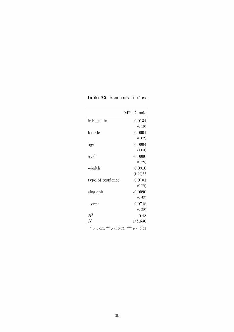
Table A2: Randomization Test

MP_female

MP_male 0.0134(0.19)

female -0.0001(0.02)

age 0.0004(1.00)

age2 -0.0000(0.28)

wealth 0.0310(1.99)**

type of residence 0.0701(0.75)

singlehh -0.0090(0.43)

_cons -0.0748(0.28)

R2 0.48N 178,530* p < 0.1; ** p < 0.05; *** p < 0.01

30

Table A3: Effects on Education - Detailed

(1) (2) (3) (4) (5) (6) (7) (8) (9)MPfemale*female 0.0091 0.0086 0.0086 0.0084 0.0022 -0.0049 -0.0045 -0.0053 -0.0052

(4.11)*** (3.57)*** (3.64)*** (3.56)*** (1.22) (1.46) (1.16) (1.31) (1.30)

MPfemale 0.0275 0.0063 -0.0036 -0.0046 -0.0032 0.0273 0.0096 0.0029 0.0016(5.50)*** (1.45) (1.14) (1.11) (0.73) (4.50)*** (1.88)* (0.79) (0.34)

female -0.1010 -0.1008 -0.1022 -0.0982 -0.0111 0.0452 0.0402 0.0409 0.0487(23.44)*** (22.65)*** (22.64)*** (14.67)*** (1.74)* (5.88)*** (5.47)*** (5.43)*** (5.62)***

number of members in hh -0.0056 -0.0040 -0.0036 -0.0044 -0.0062 -0.0048 -0.0044(5.69)*** (4.13)*** (4.08)*** (4.74)*** (5.85)*** (4.71)*** (4.76)***

type of residence 0.0155 -0.0075 -0.0079 -0.0056 0.0084 -0.0060 -0.0066(1.95)* (1.01) (1.07) (0.74) (1.34) (0.80) (0.88)

wealth 0.0744 0.0681 0.0668 0.0538 0.0614 0.0549 0.0537(22.77)*** (25.48)*** (26.58)*** (19.41)*** (18.93)*** (18.96)*** (19.47)***

MPmale -0.0050 0.0073 0.0139 0.0215 -0.0018 0.0171 0.0205(1.41) (0.65) (1.10) (1.61) (0.54) (1.51) (1.57)

age 0.0052 0.0054 0.0054 0.0841 0.1123 0.1114 0.1110(11.17)*** (11.86)*** (11.86)*** (16.86)*** (18.78)*** (18.45)*** (18.45)***

age2 -0.0002 -0.0002 -0.0002 -0.0026 -0.0030 -0.0030 -0.0030(25.79)*** (27.35)*** (27.36)*** (16.90)*** (17.70)*** (17.46)*** (17.45)***

trend -0.0000 -0.0000 -0.0000(0.29) (0.26) (0.13)

trend*female -0.0000 -0.0000 -0.0000(0.87) (1.47) (1.79)*

age2 [14-19 years] 0.1204 -0.0738 -0.0745 -0.0740(12.02)*** (8.61)*** (8.80)*** (8.92)***

age2*female -0.0904 -0.0906 -0.0904 -0.0906(6.92)*** (7.18)*** (7.14)*** (7.17)***

age2*MPfemale -0.0135 -0.0123 -0.0107 -0.0108(3.19)*** (2.93)*** (2.75)*** (2.75)***

age2*MPfemale*female 0.0117 0.0101 0.0106 0.0106(2.34)** (2.00)** (2.05)** (2.03)**

age3 [19-25 years] 0.0662 -0.1075 -0.1076 -0.1071(8.01)*** (8.79)*** (8.91)*** (8.85)***

age3*female -0.1321 -0.1260 -0.1284 -0.1280(11.68)*** (11.56)*** (11.80)*** (11.81)***

age3*MPfemale -0.0069 -0.0068 -0.0050 -0.0051(2.03)** (1.86)* (1.60) (1.60)

age3*MPfemale*female 0.0164 0.0163 0.0181 0.0178(3.54)*** (2.88)*** (2.99)*** (2.92)***

_cons 0.8101 0.6528 0.6576 0.6521 0.0607 0.7907 -0.1744 -0.1666 -0.1824(87.44)*** (29.09)*** (24.70)*** (10.94)*** (0.74) (61.08)*** (3.47)*** (3.22)*** (2.05)**

R2 0.03 0.20 0.22 0.23 0.14 0.02 0.11 0.14 0.15N 130,716 130,659 130,659 130,659 69,465 69,467 69,465 69,465 69,465Year & District FE no no yes yes yes no no yes yesYear-Region FE & Trend no no no yes yes no no no yesFull Sample yes yes yes yes no no no no no

* p < 0.1; ** p < 0.05; *** p < 0.01

31

Table A4: Effects on Female Empowerment

(1) (2) (3) (4) (5) (6) (7) (8) (9)MPfemale*female 0.0061 0.0097 0.0097 0.0095 0.0057 0.0022 0.0049 0.0051 0.0048

(3.16)*** (4.47)*** (4.35)*** (4.05)*** (1.68)* (0.97) (2.14)** (2.30)** (2.22)**

MPfemale 0.0006 -0.0020 -0.0022 -0.0020 0.0005 0.0024 0.0020 0.0021 0.0018(0.23) (0.70) (0.43) (0.34) (0.08) (0.67) (0.59) (0.31) (0.24)

female 0.0830 0.0722 0.0708 0.0718 0.0046 0.0042 0.0017 0.0011 0.0006(23.54)*** (20.89)*** (20.43)*** (13.33)*** (0.95) (0.90) (0.40) (0.26) (0.10)

type of residence -0.0555 -0.0663 -0.0680 -0.0704 -0.0588 -0.0689 -0.0701(4.36)*** (5.59)*** (5.70)*** (5.27)*** (4.21)*** (5.22)*** (5.28)***

number of members in hh -0.0022 -0.0015 -0.0013 -0.0027 -0.0034 -0.0029 -0.0028(1.82)* (1.06) (0.94) (1.81)* (2.89)*** (2.01)** (1.88)*

wealth -0.0196 -0.0235 -0.0239 -0.0250 -0.0213 -0.0249 -0.0253(6.13)*** (7.45)*** (7.59)*** (7.15)*** (6.11)*** (7.08)*** (7.23)***

MPmale 0.0047 0.0320 0.0219 0.0218 0.0034 0.0335 0.0217(1.23) (3.36)*** (2.43)** (2.31)** (0.84) (3.30)*** (2.31)**

age -0.0014 -0.0013 -0.0013 0.0104 0.0073 0.0070 0.0069(8.55)*** (8.22)*** (8.31)*** (11.80)*** (7.70)*** (7.22)*** (7.22)***

age2 0.0000 0.0000 0.0000 -0.0003 -0.0003 -0.0003 -0.0003(8.51)*** (7.95)*** (8.07)*** (9.62)*** (5.97)*** (5.59)*** (5.53)***

singlehh 0.5885 0.5829 0.5826 0.6568 0.6690 0.6619 0.6616(46.13)*** (45.69)*** (45.91)*** (56.22)*** (58.84)*** (57.31)*** (57.37)***

trend -0.0001 -0.0001 -0.0001(0.85) (0.91) (0.94)

trend*female -0.0000 0.0000 0.0000(0.26) (0.15) (0.20)

age1 [7-13 years] 0.0352 0.0007 0.0001 0.0002(6.25)*** (0.11) (0.02) (0.04)

age1*female 0.0128 0.0106 0.0119 0.0119(1.73)* (1.56) (1.73)* (1.70)*

age1*MPfemale -0.0000 -0.0010 -0.0009 -0.0008(0.01) (0.35) (0.30) (0.26)

age1*MPfemale*female -0.0070 -0.0072 -0.0079 -0.0081(1.41) (1.61) (1.74)* (1.86)*

age2 [14-19 years] 0.0499 0.0542 0.0506 0.0510(6.09)*** (4.60)*** (4.38)*** (4.46)***

age2*female 0.0097 0.0126 0.0138 0.0133(0.93) (1.24) (1.37) (1.31)

age2*MPfemale 0.0012 0.0013 0.0022 0.0018(0.37) (0.32) (0.53) (0.43)

age2*MPfemale*female -0.0001 -0.0020 -0.0009 -0.0006(0.02) (0.38) (0.20) (0.12)

age3 [19-25 years] 0.0121 0.0250 0.0237 0.0236(1.61) (1.45) (1.41) (1.42)

age3*female -0.0061 -0.0069 -0.0062 -0.0056(0.53) (0.56) (0.51) (0.46)

age3*MPfemale -0.0042 -0.0100 -0.0077 -0.0080(1.08) (1.93)* (1.24) (1.34)

age3*MPfemale*female 0.0113 0.0137 0.0134 0.0136(1.38) (1.41) (1.38) (1.42)

_cons 0.1556 0.2992 0.2305 0.1706 0.1685 0.1799 0.3058 0.2324 0.1825(30.11)*** (10.12)*** (6.90)*** (2.79)*** (2.54)** (27.81)*** (9.62)*** (6.48)*** (2.75)***

R2 0.01 0.15 0.17 0.18 0.19 0.00 0.17 0.18 0.19N 178,591 178,530 178,530 178,530 117,088 117,091 117,088 117,088 117,088Year & District FE no no yes yes yes no no yes yesYear-Region FE & Trend no no no yes yes no no no yes

* p < 0.1; ** p < 0.05; *** p < 0.0132

Table A5: Effects on Health - Detailed

(1) (2) (3) (4) (5) (6)MPfemale*female -0.00118 -0.00101 -0.00106 -0.00106 -0.00171 -0.00031

(0.00083) (0.00087) (0.00085) (0.00083) (0.00128) (0.00263)

MPfemale 0.00061 0.00046 0.00045 -0.00024 0.00440 0.00125(0.00097) (0.00094) (0.00052) (0.00083) (0.00267) (0.00156)

female 0.00313 0.00279 0.00276 0.00395 -0.00053 0.00738(0.00176)* (0.00177) (0.00175) (0.00265) (0.00214) (0.00667)

age -0.00027 -0.00027 -0.00027 0.00110 -0.00348(0.00016) (0.00016) (0.00016) (0.00143) (0.02061)

age2 0.00002 0.00002 0.00002 -0.00012 0.00011(0.00000)*** (0.00000)*** (0.00000)*** (0.00027) (0.00057)

wealth 0.00047 0.00022 0.00029 0.00020 0.00023(0.00064) (0.00060) (0.00061) (0.00065) (0.00091)

type of residence 0.00017 -0.00153 -0.00137 -0.00409 0.00220(0.00241) (0.00338) (0.00348) (0.00488) (0.00464)

number of members in hh -0.00020 0.00013 0.00013 -0.00019 0.00055(0.00027) (0.00027) (0.00027) (0.00023) (0.00037)

MPmale -0.00068 0.00015 0.00082 0.00165 -0.00041(0.00054) (0.00030) (0.00022)*** (0.00066)** (0.00041)

_cons 0.01170 0.00526 -0.00151 0.00360 -0.04116 0.01776(0.00134)*** (0.00665) (0.00792) (0.00929) (0.03229) (0.18070)

R2 0.00 0.02 0.03 0.03 0.03 0.04N 44,466 44,437 44,437 44,437 10,439 5,112Year & District FE no no yes yes yes yesYear-Region FE & Trend no no no yes yes yesFull sample yes yes yes yes no no

* p < 0.1; ** p < 0.05; *** p < 0.01

Column (5) is restricted to individuals under 7 years

Column (6) is restricted to individuals between 16 and 21 years

33

Table A6: Effects on Water - Detailed

(1) (2) (3) (4) (5) (6) (7) (8)MPfemale 0.038 -0.003 0.029 -0.002

(0.012)*** (0.009) (0.019) (0.012)

female 0.004 0.002 0.002 0.002 0.002 0.002 0.001 0.000(0.003) (0.002) (0.002) (0.002) (0.002) (0.002) (0.003) (0.003)

wealth 0.111 0.076 0.073 0.073 0.073 0.058 0.058(0.008)*** (0.005)*** (0.005)*** (0.006)*** (0.006)*** (0.008)*** (0.008)***

type of residence -0.133 -0.126 -0.125 -0.125 -0.133 -0.290 -0.296(0.043)*** (0.032)*** (0.031)*** (0.034)*** (0.034)*** (0.050)*** (0.051)***

number of members in hh -0.006 -0.001 -0.001 -0.001 -0.001 -0.005 -0.006(0.002)*** (0.002) (0.002) (0.002) (0.002) (0.002)** (0.002)**

MPmale 0.014 0.020 -0.014(0.009) (0.032) (0.031)

l1*MPfemale 0.048 0.045(0.010)*** (0.015)***

l1*MPmale -0.023 -0.017(0.013)* (0.016)

l2*MPfemale -0.074 0.147(0.015)*** (0.003)***

l2*MPmale 0.014 0.006(0.004)*** (0.003)**

_cons 0.308 0.258 0.829 1.180 0.396 0.460 0.724 0.754(0.022)*** (0.091)*** (0.098)*** (0.173)*** (0.084)*** (0.152)*** (0.101)*** (0.213)***

R2 0.01 0.17 0.36 0.40 0.30 0.32 0.46 0.47N 123,716 123,715 123,715 123,715 105,929 105,929 33,492 33,492Year & District FE no no yes yes yes yes yes yesYear-Region FE no no no yes no yes no yes

* p < 0.1; ** p < 0.05; *** p < 0.01

34

Table A7: Effects on Sanitation

(1) (2) (3) (4) (5) (6) (7) (8)MPfemale -0.034 -0.029 -0.028 0.002

(0.008)*** (0.009)*** (0.018) (0.011)

female -0.003 -0.002 -0.003 -0.003 -0.002 -0.002 -0.002 -0.003(0.003) (0.003) (0.002) (0.002) (0.002) (0.002) (0.005) (0.005)

wealth 0.012 0.007 0.005 0.001 -0.001 -0.020 -0.022(0.007)* (0.005) (0.005) (0.005) (0.005) (0.009)** (0.009)**

type of residence 0.084 0.107 0.105 0.116 0.119 0.159 0.150(0.025)*** (0.019)*** (0.018)*** (0.021)*** (0.020)*** (0.038)*** (0.037)***

number of members in hh 0.005 0.008 0.008 0.008 0.009 0.009 0.010(0.002)** (0.002)*** (0.002)*** (0.002)*** (0.002)*** (0.004)** (0.004)***

MPmale -0.003 -0.016 0.007(0.011) (0.027) (0.022)

l1*MPfemale -0.026 0.007(0.016) (0.009)

l1*MPmale -0.006 0.013(0.038) (0.018)

l2*MPfemale -0.101 0.086(0.014)*** (0.005)***

l2*MPmale -0.032 0.008(0.003)*** (0.002)***

_cons 0.470 0.255 0.571 -0.024 0.170 0.030 0.303 -0.440(0.015)*** (0.064)*** (0.068)*** (0.094)* (0.065) (0.087)*** (0.101)***

R2 0.01 0.01 0.37 0.40 0.29 0.33 0.18 0.19N 170,271 170,265 170,265 170,265 130,943 130,943 46,298 46,298Year & District FE no no yes yes yes yes yes yesYear-Region FE no no no yes no yes no yes

* p < 0.1; ** p < 0.05; *** p < 0.01

35

Figure 5: Frequency of Women by Age at First Birth

Source: DHS 2007-2008

36