Legacy Events Room CBA 3.202 11:00 am

Organizational Capital, Corporate Leadership, and Firm

Dynamics.

Wouter Dessein and Andrea Prat

Columbia University∗

July 10, 2019

Abstract

We argue that economists have studied the role of management from three perspec-

tives: contingency theory (CT), an organization-centric empirical approach (OC), and a

leader-centric empirical approach (LC). To reconcile these three perspectives, we augment

a standard dynamic firm model with organizational capital, an intangible, slow-moving,

productive asset that can only be produced with the direct input of the firm’s leadership

and that is subject to an agency problem. We characterize the steady state of an economy

with imperfect governance, and show that it rationalizes key findings of CT, OC, and LC,

as well as generating a number of new predictions on performance, management practices,

CEO behavior, CEO compensation, and governance.

∗We thank Simon Board, Jacques Cremer, Guido Friebel, Luis Garicano, Bob Gibbons, Hugo Hopenhayn,

Navin Kartik, Qingmin Liu, Michael Raith, Raffaella Sadun, John Van Reenen, Jorgen Weibull, Pierre Yared,

and participants to seminars at University of Athens, Columbia, the CMU Accounting Conference, Cowles

Foundation Summer Conference, EIEF, EUI, the Finance, Organizations and Markets conference, Johns Hop-

kins, LSE, McGill, MIT, NBER, Rochester, St Gallen, and Toulouse for useful suggestions. We are particularly

grateful to Sui Sun Cheng for his suggestions on how to analyze the recurrence equation. Sara Shahanaghi

provided excellent research assistance.

Electronic copy available at: https://ssrn.com/abstract=3024285

Legacy Events Room CBA 3.202 Thursday, October 3, 2019 11:00 am

1 Introduction

A number of empirical studies, exploiting different data sets, employing different methodolo-

gies, and covering different countries have found sizeable and persistent performance differences

between firms that operate in the same industry and use similar observable input factors (Syver-

son 2011). For instance, within narrowly specified US manufacturing industries, establishments

at the 90th percentile make almost twice as much output with the same input (Syverson 2004).

One possible explanation for this puzzling observation is that the variation in outcomes

is due to a variation in management (Gibbons and Henderson 2013). In turn, management

comprises both the management practices that firms put in place and the managerial human

capital that they employ. This paper is concerned with the question: Where do differences in

management practices and managerial capital come from?

Economists have approached this question from three different angles (summarized in

Table 1). The first approach, which we shall refer to as contingency theory (CT), is a natural

extension of production theory. Both managerial practices and managerial human capital are

production factors and the firm should select them optimally given the business environment

it faces. Lucas (1978) is the seminal application of CT to managerial human capital. There

is a market for managers where supply is given by a distribution of managers of different

talent and demand is given by a distribution of firms. In equilibrium, the more talented

managers are employed by the firms that need them more.1 CT encompasses both managerial

talent and management practices, and it can take into account synergies with other productive

factors: Milgrom and Roberts’ (1995) theory of complementarity in organizations develops

general techniques to model these synergies. CT yields two powerful testable predictions:

(i) At any point in time, if the solution to the production problem is unique, similar firms

should adopt similar management practices and should hire similar managerial talent; (ii) If

the production problem has multiple solutions, similar firms may adopt different management

practices and/or hire different managers, but this variation will not correlate with their overall

profitability. In order to get heterogeneous performance, the CT set-up can be augmented

with exogenous productivity or demand shocks, so it leads to a steady state distribution of

1As such, this model can be used to explain the allocation of CEOs to companies according to firm size (Tervio

(2008) and Gabaix and Landier (2008)) or of managerial talent within and across organizations (Garicano and

Rossi-Hansberg 2006).

1


firm size and productivity (Hopenhayn (1992), Ericson and Pakes (1995)). However, in this

case the employment of different managers or the adoption of different management practices

is an effect not a cause of differential performance: (i) and (ii) still hold.

While CT has an explicit theoretical foundation, the other two approaches are mainly

empirical. We will refer to the second one as the organization-centric empirical approach (OC).

Ichniowski et al (1997) pioneered this approach in economics. They undertook a detailed in-

vestigation of 17 firms in a narrowly defined industry with homogeneous technology (steel

finishing) and documented how lines that employed innovative human resource management

practices, like performance pay, team incentives, and flexible assignments, achieved signifi-

cantly higher performance than lines that did not employ such practices. Bloom and Van

Reenen (2007) developed a survey tool to measure managerial practices along multiple dimen-

sions. Their influential paper and subsequent work have documented both a large variation in

management practices across firms within the same industry and the ability of that variation

to explain differences between firms on various performance measures, including profitability.2

These results are robust to the inclusion of firm-level fixed effects (Bloom et al 2019) and they

survive the inclusion of detailed employee-level information (Bender et al 2018).

In sum, OC has shown that similar firms adopt different management practices and

that this difference matters for performance. As this finding is in apparent conflict with CT’s

prediction that management practices are optimally chosen, economists often react in one

of two ways. First, those seemingly similar firms may actually have different unobservable

characteristics that make it optimal for them to adopt different practices. Second, those firms

simply make mistakes and adopt the wrong practices. What both alternative explanations

have in common is they offer little in the way of empirical guidance. For the first explanation,

it would be useful to have a sense of what kind of firm-level unobservable characteristics we

should try to observe, especially given how much information we already have about those

firms. For the second, it would be good to have some kind of microfoundation for those highly

consequential errors.

The leadership-centric empirical approach (LC) focuses on the role of individual man-

agers. Some firms may perform better because they are run by better CEOs. A growing

2Graham et al. (2016), based on surveys of over 1300 CEOs and CFOs of US companies, obtain similar

results with respect to the heterogeneity and effectiveness of corporate culture. We view both management

practices and corporate culture as being part of a firm’s organizational capital.

2


literature, employing different data sets and different methodologies, show that the identity of

the CEO can account for a significant portion of firm performance (Bertrand 2009). Among

others, Johnson et al (1985) analyze the stock price reaction to sudden executive deaths,

Bertrand and Schoar (2003) identify a CEO fixed effect, and Bennedsen et al (2007) show that

family CEOs have a negative causal effect on firm performance. Kaplan et al (2012) document

how CEOs differ on psychological traits and how those differences explain the performance of

the firms they manage. Bandiera et al (2016) perform a similar exercise on CEO behavior and

show it accounts for up to 30% of performance differences between similar firms, and the asso-

ciation between behavior and performance appears only three years after the CEO is hired.3

LC can be seen as the parallel of OC, applied to managerial talent rather than managerial

practices, which raises the same set of questions: How do we reconcile the observed variation

with CT?

It is also natural to ask whether there exists a link between OC and LC.4 Are leaders and

practices two orthogonal factors that influence firm performance through distinct channels, or

are they somehow connected? For instance, do CEOs play a role in the adoption of management

practices? Or are firms with certain management practices more likely to hire a certain type

of CEO?

This paper is an attempt to reconcile these three approaches in one theoretical frame-

work. The starting point is the observation that all firms have a large, indivisible factor of

production: the CEO. CEO quality is hard to observe ex ante and even ex post, as it takes

time for him or her to affect firm performance. All firms try to hire hire a “good”CEO: some

are lucky, some are not. Firms who end up with a good CEO receive a positive and highly

persistent shock to their management practices and overall performance. Firms who, despite

their best efforts, end up with a bad CEO endure a negative and persistent shock. The paper

microfounds a world where firms face this CEO selection problem, analyzes its steady state

behavior, and relates it to the three approaches discussed above.

The objective is not to develop a general, realistic model of management and managers,

3The effect of individual leaders on organizational performance has also been documented for middle managers

(Lazear, Shaw, and Stantion 2015, Hoffman and Tadelis 2017)4 In a sample of firms where both CEO behavior and management practices are measured, Bandiera et

al (2016) find significant cross-sectional correlation between the management score and the CEO behavior,

controlling for other observables.

3


but rather to show that some of the essential lessons from CT, OC, and LC can be distilled

in a set-up that is extremely close to a standard CT dynamic firm model. There are only two

innovations. The first is a standard assumption of corporate governance theory: there is a

serious agency problem between the firm’s owner and the CEO who runs it, which creates the

potential for ineffi cient behavior on the part of the CEO (Jensen and Meckling, 1973; Tirole

2010). The nature of this problem will be discussed in more detail below.

The second innovation consists of introducing a class of firm-specific assets whose pro-

duction depends on the CEO. The performance of a firm depends on its organizational capital.

This concept is meant to encompass any intangible firm asset with four properties: (i) It affects

firm performance; (ii) It changes slowly over time; (iii) Being intangible, it is not perfectly ob-

servable; (iv) It must be produced at least partly inside the firm with the active participation

of the firm’s top management.

While conditions (i) through (iii) are familiar, condition (iv) is mostly novel to econo-

mists. It is a tenet of an influential stream of management literature that includes Drucker

(1967) and Kotter (2001). It is encapsulated in Schein’s (2010) assertion that “leadership is

the source of the beliefs and values of employees, and shapes the organizational culture of

the firm, which ultimately determines its success or failure.” In this perspective, some firms

end up with leaders who are more capable and/or willing to act in a way that increases the

firm’s organizational capital. Leadership is a flow that adds or subtracts to the firm’s stock

of intangible capital (Rahmandad, Repenning, and Henderson 2018). Note that this view of

leadership is much more precise than simply saying that some CEOs generate more profits

than others for some unspecified reason. It identifies a particular mechanism, the growth of

organizational assets, through which long-term value creation occurs in ways that lead to a

wealth of testable implications.

What could organizational capital be in practice? One possible example is the manage-

ment practices analyzed by Bloom et al. (2007), which arguably affect firm performance as

in (i) and are slow-moving as in (ii). In support of the imperfect observability condition in

(iii), note that the correlation rate of two independent and almost simultaneous measurements

of management scores within the same plant is 45.4% (Bloom et al. 2019). For (iv), Simons

(1994a) uses ten years of observational data collected in over 50 US businesses to document

how top managers use ‘control systems’, namely mechanisms for influencing human endeavor

4


within the company, to maintain or alter patterns in organizational activities; in particular,

new CEOs use their first 18 months of their tenure to define and measure critical performance

variables (Simons 1994b). There are other possible examples of organizational capital. Our

definition includes at least partially constructs such as relational contracts (Baker, Gibbons,

and Murphy 2002), corporate culture (Schein 2010), firm-specific human capital (Prescott and

Visscher 1980), or firm capabilities (Teece, Pisano, and Shuen 1997).

In the model we develop in this paper, organizational capital depreciates over time, but

the CEO can devote her limited attention to increasing it. Alternatively, the CEO can spend

her time boosting short term profit. The firm’s profit-maximizing board hires a CEO in a

competitive market for CEOs and can fire her at any time. Some CEOs are better than others

at improving organizational capital. Firms are otherwise identical. They are born randomly

and they die if their performance is below a certain threshold. There are no other factors of

production or sources of randomness.

This barebone model is completed by agency frictions. If corporate governance was

suffi ciently strong, bad CEOs could be screened before they are hired or dismissed (or persuaded

to reveal their type and resign) soon after being hired. Instead, we assume two forms of

governance problems. The firm owners face ex ante frictions: when a board hires a CEO

they have limited information about the CEO’s type, especially if the candidate has never

held a CEO’s position, namely they have an imperfect CEO screening technology. Moreover,

the board is unable or unwilling to use high-powered incentives so low-type CEOs would quit

voluntarily. The firm owners also face ex post frictions: while cash flow can be measured almost

continuously, the immaterial nature of organizational capital makes it harder to monitor. We

assume that the board observes the cash flow stream immediately , but they only spot changes

in organizational capital with a delay.

In equilibrium, firms would like to dismiss low-type CEOs but the latter hide their type

for some time by boosting short-term behavior rather than investing in organizational capital.

If the firm is lucky, it gets a good CEO who increases organizational capital and improves

long-term performance (and retires at some point). If the firm is unlucky, it gets a bad CEO

who depletes organizational capital and hurts long term performance before the firm fires her.

This implies that the organizational capital of each firm follows a stochastic process punctuated

by endogenous CEO transitions. Both sources of friction above are necessary and suffi cient to

5


generate this equilibrium.

The main technical result of the paper is the characterization of the steady state dis-

tribution of firms in this economy. We first show that the measure of firms with a certain

organizational capital is described by a recurrence equation. Although that recurrence equa-

tion is somewhat non-standard, we show that under certain assumption it has a unique steady

state, which we characterize in closed form. At every moment, there coexist firms with differ-

ent organizational capital, different leadership styles, and different performance, giving rise to

stylized OC and LC cross-sectional patterns.

The main substantive result is a set of testable implications that bring together, in

one model, some of the key patterns predicted or observed by CT, OC, and LC as well as

new implications that bring together the three approaches. On the CT front, our model

displays the performance heterogeneity and persistence predicted by Hopenhayn (1992) as well

as a power law at the top of the distribution. In OC, our analytical results are consistent

with the findings by Bloom and Van Reenen (2007) and others that (changes in) the quality

of management practices are associated with (changes in) firm performance. the quality of

corporate governance is found to play a key role. Regarding LC, we show that the CEO

behavior, type, and tenure are all predictors of firm performance, as found in the CEO

literature —with governance quality and the supply of managerial talent determining CEO

variables.

Finally, the model predicts a wealth of new cross-sectional and dynamic interactions be-

tween CT, OC, and LC concepts: the tenure, behavior, type, and compensation of present and

past firm’s CEOs predict the current level and growth rate of the firm’s organizational capital.

As before, we perform comparative statics on governance quality and leadership supply. We

also make predictions linking CEO career paths and the dynamics of organizational capital.

For instance, a firm that was run in the recent past by a CEO who is currently employed by

a larger firm should display an abnormally high growth in organizational capital and perfor-

mance. Conversely, a firm whose last CEO was short tenured will have lower organizational

capital and performance.

Of course, the model we present is not meant to be exclusive. Other factors, besides

leadership, may affect the evolution of a firm’s organizational capital. Leadership may influence

performance through channels that are distinct from organizational capital. Other frictions

6


1 2 3 4 F1 CT Seemingly identical firms display persistent

performance differences Hopenhayn (1992), Ericson and Pakes (1995), Syverson (2011)

F2 CT The right tail of the performance distribution can be approximated by a power law

Gabaix (2009), Luttmer (1995)

F3* CT CEOs and firms engage in assortative matching Gabaix and Landier (2008), Tervio (2008)

F4 OC Management practices and firm performance display positive cross sectional correlation

Ichniowski, Shaw, and Prennushi (1997), Bloom and Van Reenen (2007)

F5 OC Changes in management practices cause (and are associated with) changes in firm performance

Bloom, Eifert, Mahajan, McKenzie, Roberts (2013), Bloom, Sadun, and Van Reenen (2016)

F6 OC Firms with better governance display better management practices

Bloom and Van Reenen (2007)

F7* LC A CEO fixed effect is observable in firm performance data

Johnson, Magee, Nagarajan, Newman (1985), Bertrand and Schoar (2003)

F8 LC CEO variables (personal characteristics, behavior, etc) explain firm performance

Bennedsen, Perez-Gonzalez, Wolfenson (2007), Kaplan, Klebanov, Sorensen (2012), Bandiera, Hansen, Prat, and Sadun (2017)

F9 LC Better governance improves CEO variables and firm performance

Shleifer and Vishny (1997)

F10 new Changes in management practices are correlated with current CEO variables and CEO transitions

n.a.

F11 new Controlling (perfectly) for current management practices / organizational capital, past CEO variables do not explain current firm performance

n.a.

F12* new The employment status and compensation level of a CEO depends on the change in management practices and performance of their previous firm

n.a.

F13* new The Bertrand-Schoar approach underestimates the size of the causal effect of CEOs on performance

n.a.

Table 1: Connection between the findings of the model and selected existing literature. Column 1: Finding number (used for reference in the propositions); findings proven in the model extension are denoted with *. Column 2: Type of prediction (CT, OC, LC, or new prediction). Column 3: Informal description of the stylized pattern predicted in the model. Column 4: Selected references that discuss the patterns described in Column 3.


may affect both CEO selection and organizational capital. The goal of this paper is to see how

far we can go with a parsimonious model.

Our paper is structured as follows. The first part of the paper microfounds a dynamic

firm model. Section 2 introduces a continuous-time model of an infinitely-lived firm with or-

ganizational capital and endogenous CEO transitions. Section 3 characterizes the equilibrium

of the model when frictions are suffi ciently strong and shows that it gives rise to a stochastic

process determining CEO behavior, CEO turn-over, organizational capital, and firm perfor-

mance (Proposition 1).

Section 4 contains our main technical result: the characterization of the steady state

equilibrium of a dynamic economy with a continuum of firms that behave according to the

dynamic firm model of the previous section (Proposition 2). Given some assumptions about

firm births and deaths, the equilibrium distribution of firms obeys a recurrence equation,

whose steady state admits one closed-form solution. For suffi ciently high performance levels,

the solution satisfies an approximate power law.

Section 5 contains the main substantive results. It explores the testable implications

of the steady state characterization and shows that it reconciles key findings of CT (hetero-

geneity and persistence of firm performance), OC (cross-sectional and longitudinal relationship

between management practices and firm performance), and LC (relationship between CEO be-

havior/type and performance). The section also analyzes the role of corporate governace and

presents novel testable implications linking OC and LC variables. The predictions are related

to the existing literature (See Table 1).

Section 6 introduces observable heterogeneity in CEO quality. Suppose CEOs can live

for more than one period and work for more than one firms. The market for CEOs will then

be segmented into untried CEOs, successful CEOs, and failed CEOs. In equilibrium failed

CEOs are not re-hired, untried CEOs work for companies with low organizational capital, and

successful CEOs receive a compensation premium to lead companies with high organizational

capital. The extension leads to additional predictions: a panel regression run on data generated

by this model would yield CEO fixed effect coeffi cients; however, because of the endogenous

assignment of CEOs to companies, such coeffi cient would under-estimate the true effect of

individual CEOs on firm performance. The section also yields novel predictions on the dynamic

relationship between CEO compensation, CEO career, firm performance, and the growth of

7


organizational capital. Section 7 briefly concludes.

1.1 Literature Review

Our paper is an attempt to reconcile a number of stylized patterns, predicted by other theo-

retical papers or observed by existing empirical works. Table 1 contains a list of the patterns

that hold in our model, together with some of the papers that inspired them. The table will

be discussed in detail in Section 5.

The rest of this section relates our general approach to previous work. At least since

Hopenhayn (1992) and Erickson and Pakes (1995), economists have emphasized how firm-

specific sources of uncertainty can result in firm dynamics and long-term productivity differ-

ences between ex ante similar firms in the same industry. We follow Hopenhayn in analyzing

the steady state outcome of this dynamic process, but we micro-found one of the possible

sources of the idiosyncratic productivity shocks by introducing managerial skill heterogeneity

and moral hazard in the building of a firm’s organizational capital (management practices,

culture,. . . ). As such, we are able to link the distribution of firm productivity to corporate

governance and the supply of managerial talent, and make predictions which directly link

managerial talent with organizational capital and firm productivity.

Prescott and Visscher (1980) developed a model of “organization capital,” defined as

firm-specific accumulated information, for instance about the human capital of its employees

and the match between employees and jobs. Prescott and Visscher’s organization capital

satisfies (i), (ii), and (iii) of our definition of organizational capital above. Our model can be

thought of Prescott and Visscher with of a role for leadership, namely the addition of property

(iv) and corporate governance frictions.

Bloom et al. (2016) consider a dynamic model which —in our language —attempts to

reconcile CT with OC. Firms make costly investments in a ‘stock of management’.5 One of

the key result of the paper is that the empirical patterns they observe can be rationalized by

assuming a heterogeneous initial draw of management quality: firms are born with a random

level of management quality, and this continues with them throughout their lives. As in Lucas

5 In Bloom et al. (2016), more management is always better. They refer to this perspective as ‘Management

as a Technology’and contrast this with ‘Management as a Design’, a setting in which there are no good or bad

management practices.

8


(1978), this initial variation is not explained within the model and —to fit the data —it must

be of the same order of magnitude of the observed (endogenous) variation in management

practices. We follow Bloom et al. (2016) in thinking of management quality —an example of

organizational capital —as a slow-moving asset. However, we differ in that we fully endogenize

this asset and in so doing we create a role for corporate leadership. This has two benefits: there

is now a three-way link between CT, OC, and LC and the observed variation in organizational

capital can now be explained entirely within the model without invoking exogenous differences

between firms.

Within LC, Bandiera et al (2016) consider an assignment model where different types of

firms are more productive if they are matched to CEOs that choose the right behavior for that

firm. In the presence of limited screening and poor governance, some firms may end up with

the wrong CEO, thus generating low performance. This paper uses a similar building block,

but combines it with organizational capital in a dynamic firm model and studies steady-state

properties.

On the theory front, a number of models explore reasons why similar firms may end up

on different performance paths. Li, Matouschek and Powell (2017) show how performance dif-

ferences between (ex ante) identical firms may arise because of path-dependence in (optimal)

relational contracts. In Chassang (2010) differences in a firm’s success in building effi cient

relational contracts determines productivity differences. In Ellison and Holden (2014) path

dependence in developing effi cient rules for employee behavior also result in performance dif-

ferences . Halac and Prat (2016) assume the presence of a costly but imperfectly observable

monitoring technology that must be maintained by top management: some firms end up in in

persistent low-trust, low-productivity situations. Board et al. (2016) propose a model where

firms with higher levels of human capital are better at screening new talent, creating a positive

feedback loop. In Powell (2019), firms which earn higher competitive rents have the credibility

to adhere to more effi cient relational contacts with their employees, creating a positive feedback

loop.

None of the above papers has a role for personal leadership. In contrast, in our model

path dependence in productivity stems from the effect of the type and behavior of individual

CEOs on the accumulation of organizational capital. Our approach is closest to Rahmandad,

Repenning, and Henderson (forthcoming), who model the firm’s capability as an asset whose

9


rate of change depends on the behavior of the firm’s leader: a short-term behavior leads to

slower capability accumulation. More broadly, our paper is inspired by models of corporate

leadership where leaders have a ‘type’that affects their performance (e.g. Van den Steen 2005,

Bolton et al. 2012, Hermalin 2013), or they have beliefs that are reflected in the strategy they

develop (Van den Steen 2018), or they influence the shared frames that affect performance

(Gibbons, LiCalzi, and Warglien 2017).

A recent paper by Besley and Persson (2018) studies organizational culture from a differ-

ent angle. They analyze the transmission of cultural values in organizations with overlapping

generations of managers. They show how organizational culture becomes a natural source

of inertia and prevent organizations from responding to shocks in their environment, thus

explaining phenomena such as dysfunctional cultures and resistance to change.

Our paper is related to a literature in corporate finance on managerial short-termism

(Stein 1989). Most of this literature is focused on how different financial contracts (e.g. short-

term versus long-term debt) trade-off a desire for early termination of unprofitable projects

with the need to provide adequate incentives for long-term investments (Von Thadden (1995)).

In contrast, we study the consequences of heterogeneity in managerial short-termism on the

productivity dispersion of ex ante identical firms. Indeed, in our paper, bad managers are able

to temporarily mimic the performance of good managers by boosting short-term performance

at the expense of long-term investments in organizational capital. Our model further differs

from classic models of managerial short-termism in that only bad managers engage in short-

term behavior.

Finally, our paper is also loosely linked to a long-standing debate on the role of individual

leaders in determining the evolution of institutions (summarized in Jones and Olken 2005, who

also measure the causal effect of individual leaders). At one extreme, a certain interpretation

of Marxism sees leaders as mere expressions of underlying social phenomena and structures:

the latter are the real drivers of historical change with individuals being essentially fungible.

At another extreme, traditional historiography often ascribes enormous importance to the

behavior of great leaders, who are credited with single-handedly changing the course of history

by developing or destroying institutions.

10


2 A Dynamic Model of Firm Performance

We propose a dynamic model of an industry composed of a mass of individual long-lived firms.

Each firm is defined by its organizational capital and faces an agency problem.

Specifically, a firm’s profit at time t is a function of the firm’s organizational capital

Ωt. This organizational capital includes the quality of the firm’s management practices and

management system, its culture and norms and so on. The firm has a CEO whose responsibility

it is to maintain and grow this organizational capital, denoted as behavior x = 1, but can shirk

on this responsibility and engage instead in activities which boost short term performance,

denoted as behavior x = 0.6

In the long-term behavior (x = 1), the CEO might be building a management system

and provides supervision and motivation to workers. In the short-term behavior (x = 0), the

CEO might instead spend her time boosting productivity immediately. For example, the CEO

could be monitoring operations directly as opposed to creating an accountability system, or

going on sales pitches as opposed to incentivizing/training sales managers. Central to our

analysis is that there are two types of CEOs, good and bad, who differ in their managerial

ability to build organizational capital.

Formally, the firm’s performance or flow profit at time t is given by

πt = (1 + b (1− x)) Ωt, (1)

where b ∈[0, b]is a short-term boost to performance, as chosen by a CEO engaging in behavior

x = 0. The firm’s organizational capital is an asset that evolves according to:

Ωt = (θx− δ) Ωt,

where δ is the depreciation rate of managerial capital and θ ∈θL, θH

represents the CEO’s

managerial skill with θH > θL.

The model could easily be extended to include other production factors. For instance,

one might have a standard formulation in which

πt = (1 + b (1− x)) Ωtf (Kt, Lt)− rKt − wLt − F, (2)

6One key simplifying assumption is that the CEO chooses her behavior once and for all at the beginning of

her tenure. The assumption is discussed —together with other limitations of the model —after Proposition 1.

11


where Kt is the amount of capital and r is its unitary cost, Lt is the amount of labor and w

is its unitary cost, and F is a fixed cost. With this formulation, Kt and Lt would be chosen

given the firm’s organizational capital. Under standard assumptions, the optimal amount of

capital and labor would be increasing in the value of the firm’s organizational capital. The

results presented in the rest of the paper would continue to hold, with minimal modfications.

To keep notation to a minimum we abstract from other factors and use (1).

The owner (or board) maximizes long-term profits∫ ∞0

e−ρtπtdt

We assume that behavior 1 is optimal for both CEO types (θL large enough compared

to b). Hence, if the owner observed the CEO type she would always hire the high type and

instruct her to choose x = 1.

The owner, however, does not observe the CEO type, the CEO’s behavior x ∈ 0, 1, orthe current level of the organizational capital immediately. They are observable with a delay

R. The only variable the owner observes in real time is performance

The board appoints the CEO and she can fire him whenever she wants, but CEOs must

retire after time T. The probability of selecting a high type θH is given by p > 0.

CEO’s do not care about profits, but maximize tenure. When hired, the CEO chooses

a management style and —for simplicity —we assume she cannot change it over time. We will

discuss the relevance of this assumption in the next section.

We assume there is a continuum of firms. Each firm’s life is governed by the following

birth and death process:

Assumption S1: A firm dies whenever its performance is smaller or equal than a certain

profit level π0.

Assumption S2: At each moment a mass B of new firms are born as spin-offs of existing

firms. The spin-offs are clones of existing transitioning firms (firms who are changing their

CEOs) and they inherit the organizational capital level of the firm they originate from.

At each instant, we assume events occurs in the following order: (i) if optimal or nec-

essary, firms replace their CEO, (ii) firms with performance smaller or equal than π0 die, (ii)

a mass B of new firms are born as spin-offs of existing transitioning firms. The goal of our

12


analysis is to characterize the steady state equilibrium of an industry with a mass of firms that

follow the assumptions above.

2.1 Remarks about Modeling Choices

The objective of this paper is to introduce a simple model that gives rise to steady state

behavior that replicates the stylized patterns summarized in Table 1. Other modeling choices

are possible, but we have discarded them either because they lead to a set-up that is not

solvable analytically or because they do not yield some of the desired steady state pattens.

Here, performance is perfectly observed while CEO behavior and organizaional capital

are completely unknown at least for period R. More realistically, we could have assumed that

some or all of these variables are observed with some noise, perhaps following the continuous-

time Brownian motion set-up introduced by Sannikov (2007). Unfortunately, these formulation

does not appear to lead to a tractable steady-state characterization.

Alternatively, one could look for a basic discrete-time formulation, where CEOs are in

charge for one period and can be bad or good. While this assumption would lead to an even

more tractable set-up, this non-microfounded approach would not generate many of the desired

steady state patterns. The effect of corporate governance on steady state variables would have

to be assumed in an ad-hoc manner. Unless more ad hoc assumptions are added, the model

would also be silent on the role of CEO behavior, on the equilibrium relationship between CEO

tenure and other variables, and on a number of other equilibrium relationships discussed in

Section 5.

The assumptions about the death and birth processes (S1 and S2) are not crucial to

the results. One could complicate the model by assuming that death occurs probabilitically

at different levels or that birth occurs with a different probability distribution. The analysis

would become more complex and probably require a numerical approach. One could simplify

the birth process by assuming that a mass of firms are born in every period at a given level. This

too would lead to an analytical characterization of the steady state. However, the equilibrium

distribution would display an unrealistic spike in correspondence of the birth level.

13


3 CEO Behavior, CEO Turnover and Firm Performance

We first present the results of our simple model, which is based on a number of stark assump-

tions. At the end of the section, we discuss how robust the results are to modifications of the

assumptions.

To gain intuition, suppose all CEOs behave naively. They all choose optimal behavior:

x = 1. Managerial capital growth then equals

Ωt = (θ − δ) Ωt,

and is thus faster for θH than for θL. As performance is given by πt = Ωt, the performance

growth rate isπtπt

= θ − δ

Note that in the latter case, the low type would immediately be spotted and fired. As we

show next, this cannot be an equilibrium, as a low type CEO then has an incentive choose the

short-term behavior.

Consider the case where good CEOs choose x = 1, but bad CEOs choose the short term

behavior x = 0. While this causes organizational capital to depreciate, it allows the bad CEO

to mimic the performance of good CEOs for a while. Normalizing t to 0 at the time of CEO

hire, profits at time t ∈ [0, T ] are given by

πHt = ΩHt = Ω0e

(θH−δ)t

for the high type, whereas

πLt = (1 + b) ΩLt = (1 + b) Ω0e

−δt

for the bad type.

As long as(1 + b

)ΩLt ≥ πHt , the bad type can mimic the good type by choosing a

short-term boost b ∈[0, b]so that πLt = πHt . Mimicking becomes unsustainable after a period:

K =ln(1 + b

)θH

.

Throughout the analysis, we assume that

T > K. (A1)

14


It follows that CEO type is identified for sure after K periods. That may come before or after

the exogenous observational delay R. So, a bad CEO is fired after a period of t = min (K,R).

Good CEOs are kept until retirement (T > t). Clearly, the above behavior is an equilibrium.

The following result holds:7

Proposition 1 A low-type CEO chooses behavior 0, is fired after a period t = min (K,R) with

K =ln(1+b)θH

, and leaves a firm with a worse management system:

ΩLt = Ω0e

−δt < Ω0.

A high-type CEO chooses behavior 1, serves until retirement, and leaves a firm with a better

management system:

ΩHT = Ω0e

(θH−δ)T .

To illustrate the proposition, assume that Ω0 = 1, θH = .10, δ = .06, ρ = .05, ln(1+ b) =

.20, R = 3, and T = 5. We therefore have that

t =.20

.10= 2

so that a bad manager leaves after two years and leaves organizational capital that is e−(.06)2 =

0.886 times the capital she found. A good manager retires after 5 years and leaves an organi-

zational capital that is e(.04)5 = 1.221 times what she found.

Figure 1 plots the organizational capital and Figure 2 the performance of a firm that

hires a bad CEO, followed by another bad CEO, followed by a good CEO, followed by a bad

CEO.

[W*] Every time a bad CEO departs, the model predict a sharp drop in observed per-

formance. These stark jumps can be interpreted at face value as accounting restatements of

financial performance (Hennes et al. (2008) document the correlation between financial re-

statements and CEO turnover) or, more likely, they should be taken with a grain of salt as an

artifact of a model where performance is perfectly observable (see the discussion of assumptions

below). In a richer model, the drops would probably be replaced by declines.

7 It is easy to see this is the only equilibrium where a good CEO chooses x = 1. There are also (less plausible)

equilibria where the CEO always chooses x = 0, and any upward deviation in performance is interpreted as

coming from a bad CEO.

15


0 1 2 3 4 5 6 7 8 9 10 110.0

0.2

0.4

0.6

0.8

1.0

1.2

1.4

t

Figure 1: Organizational capital Ωt over time

0 1 2 3 4 5 6 7 8 9 10 110.0

0.2

0.4

0.6

0.8

1.0

1.2

1.4

t

Figure 2: Performance πt over time

16


Proposition 1 depends on a number of stark assumptions we have made. As mentioned

in the introduction, the results hinge on the presence of a serious agency problem within

the company. In a frictionless environment, bad CEOs would either not be hired or leave

immediately, in which case CEOs would only be high quality and there would be no leadership

heterogeneity. Let us go over the various frictions we have assumed.

First, we posited that the owner is unable to screen CEOs based on their quality θ. If the

owner had an effective screening technology, she would only hire the good ones. The extension

of the model (Section 6) with various quality levels explores the possibility that CEOs can

move from one firm to the other, in which case owners can learn something about the CEO’s

type from the performance of the firm they worked for previously.

Second, we assumed that the CEO receives a flat wage (normalized to zero). If the CEO’s

contract included a suffi ciently strong performance-contingent component, a bad CEO could be

incentivized to reveal his type right away.8 This assumption can be assessed from a pragmatic

perspective or a theoretical one. First and foremost, in practice it has been argued that, even

in developed market economies such as the US, corporate governance is highly imperfect: the

actual incentive schemes that CEOs receive are highly constrained and they do not align the

CEO’s interest with that of the firm (Bebchuk 2009). From a theoretical perspective, one can

also show that enlarging the set of contracts available to the company may not weed out bad

CEOs, because the incentive schemes that achieve this goal also increase the rent the firm must

concede to all CEOs. This point is explored formally in Appendix II.

Third, we assumed that the owner does not observe organizational capital Ωt directly.

Obviously, if she does, she could kick out a bad CEO immediately. One could consider an

alternative model where the owner observes a noisy continuous signal of organizational capital

and will fire a CEO if enough evidence accumulates. The results would be qualitatively similar

to the present model (but the analysis would be more complex —prohibitively so, at least for

us, when we move to the aggregate level).

Fourth, we assumed that the owner observes cash flow perfectly. This assumption too

could be relaxed. As in the previous point, the resulting model would be much more com-

plex. Having imperfectly observable performance would eliminate the stark negative effect on

8For instance, suppose the CEO is offered a large stock option plan (a share of future profits): then, a bad

CEO would rather resign right away in the hope that his replacement is of greater quality. It is possible to think

about other schemes that would achieve the same result, like a golden parachute, backloaded compensation, etc.

17


performance that we currently observe when a bad CEO departs.

Finally, we assumed the CEO cannot change her management style over time. This leads

to equilibrium uniqueness. If the CEO were to be able to change her behavior over time, the

equilibrium of Proposition 1 would still exist, but other perfect Bayesian equilibria may arise

too. The good CEO could signal her type by first playing x = 1, then plays x = 0 before

reverting back to x = 1. Since it would be suffi cient for the good CEO to play x = 0 for

an infinitesimal time, separation could occur (almost) immediately and a bad type would be

fired (almost) instantly. Those immediate signaling equilibria would mainly be an artifact of

our assumption that profits are perfectly observable and predictable. Unfortunately, adding

noise to performance renders the analysis unwieldy very quickly. A more tractable way to

eliminate signaling equilibria is to assume that the bad type is more productive at the short

term behavior, that is b ∈bL, bH

and the CEO’s type is either (θL, bH) or (θH , bL).9 Our

assumption that CEOs needs to commit to a particular management style once hired achieves

the same goal and keeps the model simple.

4 Steady-State Distribution of Organizational Capital

Now that we have characterized the equilibrium behavior of an individual firm, we analyze

aggregate behavior. Our goal is to characterize the steady state distribution of firms across

organizational capital levels.

We proceed in two steps. First, we characterize the steady state in the non-generic case

where the primitives of the problem are such that the distribution of firm performance has no

drift. Second, we extend it to the case with drift. As most of the analytical complexity is in

the first step, the analysis is easier to follow if one abstracts from drift.

4.1 Steady State Analysis: Good and Bad CEOs Have Same Absolute Effect

We first perform the analysis under a simplifying assumption:

9Without loss of generality, one could also introduce a third type of manager (θL, bL) which is lousy at both

behaviors. It suffi ces then that both other types engage in signalling for a (infinitessimal) short time right after

being hired, for such a type to be immediately discovered and fired.

18


0 1 2 3 4 5 6 7 8 9 10 110.4

0.6

0.8

1.0

1.2

1.4

1.6

t

Figure 3: Possible organizational capital paths. Thick black line represents possible paths of

organizational capital Ωt over time. Each bifurcaction point corresponds to a CEO transition

where the firm can either draw a good CEO or a bad CEO. The thin red lines illustrate how

under Assumption S3 organization capital is at the same level after one bad CEO and one

good CEO.

Assumption S3: The effect of a bad CEO exactly undoes the effect of a good CEO :

Ωte(θH−δ)T e−δt = Ωt

⇐⇒ (θH − δ)T = δt

Assumption S3 combined with Proposition 1 implies that all firms will experience tran-

sitions at a stable countable number of organizational capital levels. This greatly simplifies

the exposition of the results.

The extension of the findings to cases beyond S3 involves a time-dependent rescaling

of organizational capital. We will present it in the next section, once the baseline case is

understood.

Figure 3 illustrates possible organizational capital paths when Ω0 = 1. Thanks to S3,

all CEO transitions occur at a countable number of time-invariant levels.

We begin by defining the distribution of active firms. Let φ : [0,∞) × [0,∞) → <+ be

an integrable non-negative function: φt (Ω) denotes the measure of firms with organizational

19


capital Ω active at the start of time t.10 While we refer to φ, and analogous objects, as

“distributions,” note that these are not probability distributions because their integral does

not equal one: the mass of firms active at time t is∫∞

0 φt (Ω) dΩ. We adopt the convention

that φt (Ω) only includes existing firms, and does not include any firms born at time t .

Let a steady state distribution, if it exists, be denoted with φ (Ω). This is the object we

are trying to characterize.

At any CEO transition, performance πt and organizational capital Ωt are equal and fully

known to the firm. The countable set of organizational capital levels at transition is thus the

same as the countable set of performance levels at transitions, which we now define formally.

From S1, there is a lowest performance level at CEO transitions, which we denote by π0.

Starting from this lowest performance level, construct a set of transition organizational capital

levels Π as follows:

Π =

Ω : ∃j ∈ N such that Ω = Ωj ≡ π0(1 + ∆)j

where ∆ is the percentage improvement in organizational capital following a good CEO

1 + ∆ ≡ e(θH−δ)T .

Assumption S3 and Proposition 1 imply:

Lemma 1 A firm born with organizational capital Ωj ∈ Π can experience a CEO transition

only at organizational capital levels in Π. Moreover, for any organizational capital level Ωj ∈ Π,

a firm born with organizational capital in Π has a strictly positive probability of transitioning

at Ωj at some point during its lifetime.

Given the function φ, we can define g : [0,∞) × N → <+ as gt (j) = φt (Ωj) for all

Ωj ∈ Π and all t ≥ 0. The new function g represents the distribution of transitioning firms

over all possible transition organizational capital levels Ω1,Ω2,Ω3, .... The total measure of

firms transitioning at t is

Gt =∞∑j=0

gt (j) .

10We focus on atomless distributions because the steady state distribution over organizational capital cannot

contain atoms. By Proposition 1, an atom at t for a given organizational capital would generate at least one

atom an instant later, either at a slightly higher level or a at a slightly lower level — thus giving rise to a

contradiction.

20


In steady state, we can interpret Gt = G as the mass of firms that have a CEO transition

per unit of time, in the same way B equals the mass of firms that are born per unit of time.

Similarly, we can interpret gt(j) = g(j) as the mass of firms that have a CEO transition at

organizational capital level j per unit of time. Hence, B, Gt and gt(j) can best be understood

as ‘rates’, as at any instant, a mass zero of firms has a CEO transition.

From assumption S2, a measure B of new firms are born at each instant and spread

across organizational capitals Ωj ∈ Π in proportion to the measure gt(j) of existing firms at

those levels. Hence, the measure of transitioning and newly-born firms with organizational

capital Ωj at time t equals

(1 +B/Gt)gt(j) (3)

Our aim is to characterize φ(Ω), the steady state distribution of existing firms over all

organizational capital levels Ω ∈ (π0,+∞]. We take the following approach:11

1. We first characterize g (j) , the steady state distribution of existing firms over organi-

zational capital levels Ωj ∈ Π (Proposition 2). Given Proposition 1 and Assumption

S2, this is also the steady state distribution of the subset of firms experiencing a CEO

transition.

2. The steady distribution of firms over all organizational capital levels, φ(Ω), then follows

mechanically from g (j) and the equality φ(Ωj) = g (j) for all j ∈ N.

Consider the subset of firms with organizational capital Ωj ∈ Π. An existing firm that

finds itself at organizational capital level Ωj at time t must belong to one of the following

two cases: (i) It is a firm undergoing a CEO transition, and the last CEO was bad. This

means that at time t − t, the firm had organizational capital level Ωj+1. (ii) It is a firm

undergoing a CEO transition, and the last CEO was good. This means that at time t−T , thefirm had organizational capital level Ωj−1. Hence, using (3), the measure of existing firms at

organizational capital level Ωj at time t is given by

11We choose the set Π because it is the simplest of its kind. One can of course make other assumptions on

the set of performance levels at which firms can transition. It is easy to see that no such set can have a smaller

cardinality than (the countably infinite set) Π. In fact, any such set can be expressed as a (possibly infinite)

combination of sets of the form Π with different lowest performance levels π0.

21


gt (j) = (1− p)(

1 +B

Gt−t

)gt−t (j + 1) + p

(1 +

B

Gt−T

)gt−T (j − 1) (4)

The expression in (4) is a recurrence equation in two dimensions, j and t. However, it

is non-standard because: (i) it combines a discrete dimension j with a continuous dimension

t; (ii) gt (j) depends on two sets of past values of g, taken at two different times (gt−T (j − 1)

and gt−t (j + 1)); and its right-hand side contains two variables that depend on a summation

of past variables (Gt−T and Gt−t).

To make progress, we use (4) to create a new recurrence equation that applies to “even

CEO transitions”, namely the set of organizational capital levels Ω0, Ω2, Ω4, etc:

ΠE =

Ω : ∃k ∈ N such that Ω = π0(1 + ∆)2k

We define a new function ft (k) = gt (2k) for k = 1, ... This will help us characterize the

steady state. Suppose that the whole system is in a steady state, namely φt (Ω) = φ (Ω) and

Gt = G for every t. Then, it is also true that ft (k) = f (k) for every t.

We can show that a necessary condition for steady state is a one-variable difference

equation:

Lemma 2 In steady state, the following conditions must be satisfied for some γ > 0:

• A difference equation:

f (k) = (1 + γ)(p2f (k − 1) + 2 (1− p) pf (k) + (1− p)2 f (k + 1)

)for every k ≥ 1.

(5)

• Two boundary conditions:

f (0) = 0

f (1) =B

(1 + γ)(1− p)2

Proof. By applying (4) twice, we obtain

gt (j) =

(1 +

B

Gt−T

)pgt−T (j − 1) +

(1 +

B

Gt−t

)(1− p) gt−t (j + 1)

=

(1 +

B

Gt−T

)p

((1 +

B

Gt−2T

)pgt−2T (j − 2) +

(1 +

B

Gt−t−T

)(1− p) gt−t−T (j)

)+

(1 +

B

Gt−t

)(1− p)

((1 +

B

Gt−t−T

)pgt−t−T (j) +

(1 +

B

Gt−2t

)(1− p) gt−2t (j + 2)

)22


In steady state, it must be that gt (j), and thus Gt are constant over time. Dropping

time subscripts and defining

γ =

(1 +

B

G

)2

− 1,

the expression above simplifies to

g (j) = (1 + γ)(p2g (j − 2) + 2p (1− p) g (j) + (1− p)2 g (j + 2)

)When we re-write it in terms of f we obtain the first part of the lemma.

The first boundary condition is by definition. For the second boundary condition, note

that the measure of dying firms must equal the measure of new born firms B. If a firm dies at

time t, this means that at the end of time t− t, this firm had a bad CEO and organizational

capital level Ω1. It follows that the total measure firms dying at time t is given by

(1− p)(

1 +B

Gt−t

)gt−t (1)

Applying (4) to gt−t (1) and taking into account that gt−2t (0) = 0, we can rewrite this as

(1− p)2

(1 +

B

Gt−t

)(1 +

B

Gt−2t

)gt−2t (2)

Hence, in steady state, we must have that

(1− p)2

(1 +

B

G

)2

g (2) = B

⇐⇒ (1 + γ)(1− p)2f (1) = B

The difference equation (5) expresses the measure of firms at organizational capital level

j = 2k, as a function of the measure of firms at levels 2(k+ 1),2k, and 2(k− 1). A firm at level

Ωj must belong to one of the following four cases: (i) It was at level 2(k + 1) two transitions

earlier and got two bad CEOs; (ii) It was at 2k two transitions earlier and got a bad CEO and

a good CEO in either order; (iii) It was at 2(k − 1) two transitions earlier and got two good

CEOs; (iv) It was born in the preceding CEO transition or the one before that from a firm in

(i), (ii), or (iii)

Case (iv) yields the term (1 + γ) in equation (5). Recall that G =∑

jg (j) is the

steady-state measure of transitioning firms. In the proof of Lemma 2 we see that

1 + γ =

(1 +

B

G

)2

,

23


namely γ can be interpreted as the expected firm birth rate over two transitions.12 We will

henceforth simply refer to γ as the birth rate. If γ were an exogenous parameter, equation

(5) would be a relatively standard second-degree difference equation in k. Unfortunately, as

we discuss below, (5) does not pin down γ which is an endogenous variable. This complicates

things considerably.

We assume that p < 1/2. If the share of good CEOs is larger than 50%, it is easier to see

that there is no steady state as the average firm does better and better over time. Instead if

most CEOs are bad, individual firms are worsening over time on average and they eventually

die: a steady state exists because some firms do well in the medium term and new firms are

born.

Recurrence equations are sometimes used to represent heat diffusion processes in discrete

time: a solid is subject to heating and cooling sources and we are interested in knowing the

steady state temperature of different discrete points of the solid. One may wonder whether

our problem corresponds to known diffusion problems. In this perspective, (5) can be loosely

interpreted as a discrete version of the heat diffusion process of an imaginary one-dimension rod,

with some additional features: (i) The rod begins at zero on the left side and it is unbounded

on the right side; (ii) The diffusion parameter is asymmetric (as p < 12 , heat tends to flow left

rather than right); (iii) The rod is heated along its length in a way that increases temperature

at every point by rate γ per period; (iv) The total amount of added heat is constant (making

γ endogenous) (iv) The left end of the rod is next to a powerful cooling source that keeps the

temperature at zero. While this process is reminiscent of well-studied processes (especially in

a continuous setting), we are not aware of any existing result that is directly applicable to the

discrete case we are studying.

The characterization of f (·), proven formally in the Appendix, proceeds in a number ofsteps. We begin with the solution to the difference equation (5) when we treat the birth rate

γ as an exogenous parameter. Together with the boundary conditions on the death threshold

and the mass of births, it is easy to show this difference equation has a unique, distinct solution

for every possible value of γ provided p < 1/2 (the value of B just determines a rescaling of

the whole distribution).

The proof then shows that this solution for f (·) has a positive value for all k > 0 if and

12This condition has already been used to derive the second boundary condition. Thus, adding it to the set

of conditions in Lemma does not reduce the set of solutions of the difference equation.

24


only if γ ∈ (0, γ∗] where

1 + γ∗ ≡ 1

1− (1− 2p)2

In economic terms, a steady state cannot exist if the size of the economy, as proxied by

Gt =∑

j gt(j), is small relative to constant inflow of new firms B, that is whenever 1 + γt ≡(1 +B/Gt)

2 > 1 + γ∗. Intuitively, given an exogenous influx of new firms, we expect the econ-

omy to keep growing until Gt is suffi ciently large and the (endogenous) number of deaths equal

the (exogenous) number of births.

While the difference equation (5) provides a distinct solution to f (·) for each γ ≤ γ∗,

a simple refinement narrows the set of steady states down to one. Note that in steady state,

we must have that limk→∞ f(k) = 0.13 Consider therefore the N -level version of our problem

where we impose the boundary condition ft(k) = 0 for k > N with N a finite positive integer.

In this finite version of our problem, organizational capital is bounded above by Ω = ΩN .

Definition 1 We say that a steady state is reachable from below if can be the limit of a

sequence of steady states of the finite N -level version of our problem when N →∞.

This refinement excludes steady states that cannot be found as the limit of a sequence

of steady states of the finite version of our problem when the upper bound goes to infinity.

Intuitively, those steady states require a “large mass”of firms with high levels of organizational

capital. That is why they cannot be approximated by steady states of problems with an upper

bound, no matter how high the upper bound is.14

In the appendix, we show that in any finite version of our original problem the birth

rate cannot be lower than γ∗. Formally, this is proven by deriving an upper bound to the

eigenvalue of the transition matrix. If it were lower than that, then intuitively a steady state

could not exist because the mass Mt of transitioning firms would be decreasing. This proves

that a necessary condition for a steady state to be reachable from below is that in equilibrium

the birth rate is exactly γ∗.

Once the value of 1 + γ∗ ≡ 1/(

1− (1− 2p)2)is plugged into the general solution of (5),

13 If not, the mass of transitioning firms M is infinite, which cannot be a steady state.14Consistent with this, our numerical simulations indicate that only the steady state where γ = γ∗ is reached.

25


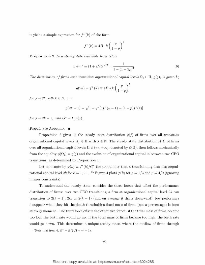
it yields a simple expression for f∗ (k) of the form

f∗ (k) = 4B · k(

p

1− p

)kProposition 2 In a steady state reachable from below

1 + γ∗ ≡ (1 +B/G∗)2 =1

1− (1− 2p)2 . (6)

The distribution of firms over transition organizational capital levels Ωj ∈ Π, g(j), is given by

g(2k) = f∗ (k) ≡ 4B ∗ k(

p

1− p

)kfor j = 2k with k ∈ N, and

g(2k − 1) =√

1 + γ∗ [pf∗ (k − 1) + (1− p)f∗(k)]

for j = 2k − 1, with G∗ = Σjg(j).

Proof. See Appendix.

Proposition 2 gives us the steady state distribution g(j) of firms over all transition

organizational capital levels Ωj ∈ Π with j ∈ N. The steady state distribution φ(Ω) of firms

over all organizational capital levels Ω ∈ (π0,+∞], denoted by φ(Ω), then follows mechanically

from the equality φ(Ωj) = g(j) and the evolution of organizational capital in between two CEO

transitions, as determined by Proposition 1.

Let us denote by ϕ(k) ≡ f∗(k)/G∗ the probability that a transitioning firm has organi-

zational capital level 2k for k = 1, 2., ...15 Figure 4 plots ϕ(k) for p = 1/3 and p = 4/9 (ignoring

integer constraints):

To understand the steady state, consider the three forces that affect the performance

distribution of firms: over two CEO transitions, a firm at organizational capital level 2k can

transition to 2(k + 1), 2k, or 2(k − 1) (and on average it drifts downward); low performers

disappear when they hit the death threshold; a fixed mass of firms (not a percentage) is born

at every moment. The third force offsets the other two forces: if the total mass of firms became

too low, the birth rate would go up. If the total mass of firms became too high, the birth rate

would go down. This determines a unique steady state, where the outflow of firms through

15Note that from 6, G∗ = B/(√

1 + γ∗ − 1).

26


0 1 2 3 4 5 6 7 8 9 10 11 12 13 14 150.00

0.02

0.04

0.06

0.08

0.10

0.12

0.14

k

Figure 4: Probability distribution ϕ(k) ≡ f∗(k)/G∗ (ignoring integer constraints) of transi-

tioning firms, and this for p = 1/3 (black line) and p = 4/9 (red line).

death equals the outflow of firms through birth and the organizational capital distribution

replicates itself over time.

The steady state distribution has the following properties:

Corollary 1 The steady state distribution of (even) transitioning firms, f(k) :

• Is single-peaked, with modal performance level km = arg maxk f∗ (k) increasing in p.

• Shifts to the right in the sense of first-order stochastic dominance as p increases:

d

dpF ∗(k) < 0 for all k ≥ 1

where F ∗(k) is the cumulative probability distribution:

F ∗(k) ≡

∑l≤k

f(l)∑lf(l)

= 1−(

p

1− p

)k (1 + k

1− 2p

1− p

).

• Follows a power-law at the right tail (top performers): There exists a c > 0 such that for

k large f(k) ≈ c ∗ Ω−ζk with ζ = 12 ln(1+∆) ∗ ln 1−p

p

27


10 15 20 25 30 35 40 45 500.00

0.01

0.02

0.03

0.04

0.05

0.06

0.07

Figure 5: The black curve plots the frequency distribution φ(Ωk) for Ωk ≥ 10 (parameters:

Ω0 = 1, ∆ = 0.2 and p = 1/3). The red curve plots the asymptotic power- law distribution

c ∗ Ω−ζk with ζ ≈ 1.9.


A well-documented empirical regularity on firm dynamics is that the right tail of the firm-

size distribution follows a power law (Gabaix 2009, Luttmer 2010). In line with this observation,

Proposition 2 implies that the right tail of the distribution of organizational capital follows

a power law. Figure 5 illustrates the convergence of the organizational capital distribution

to a power law for large levels of organizational capital. The power law approximation is a

consequence of the underlying microfoundation, whereby performance follows a Markov chain.

Corollary 1 implies that economies with, on average, higher organizational capital have

a performance distribution whose mode is shifted to the right. This result is consistent with

the findings by Bloom et al. (2016) on management practices across countries. While this

result is intuitive and appealing, we note that steady state models where new firms are born

with some exogenous organizational capital level would not deliver this result. Instead, the

modal firm in such models cannot have a higher organizational capital in steady state than

the organizational capital level at which firms are born, which is inconsistent with the findings

28


by Bloom et al. (2016).16

4.2 Steady State: Good and Bad CEOs Have Different Absolute Effects.

The previous analysis was performed under Assumption S3, which states that the positive

effect on organizational capital of a good CEO is exactly undone by the negative effect of a

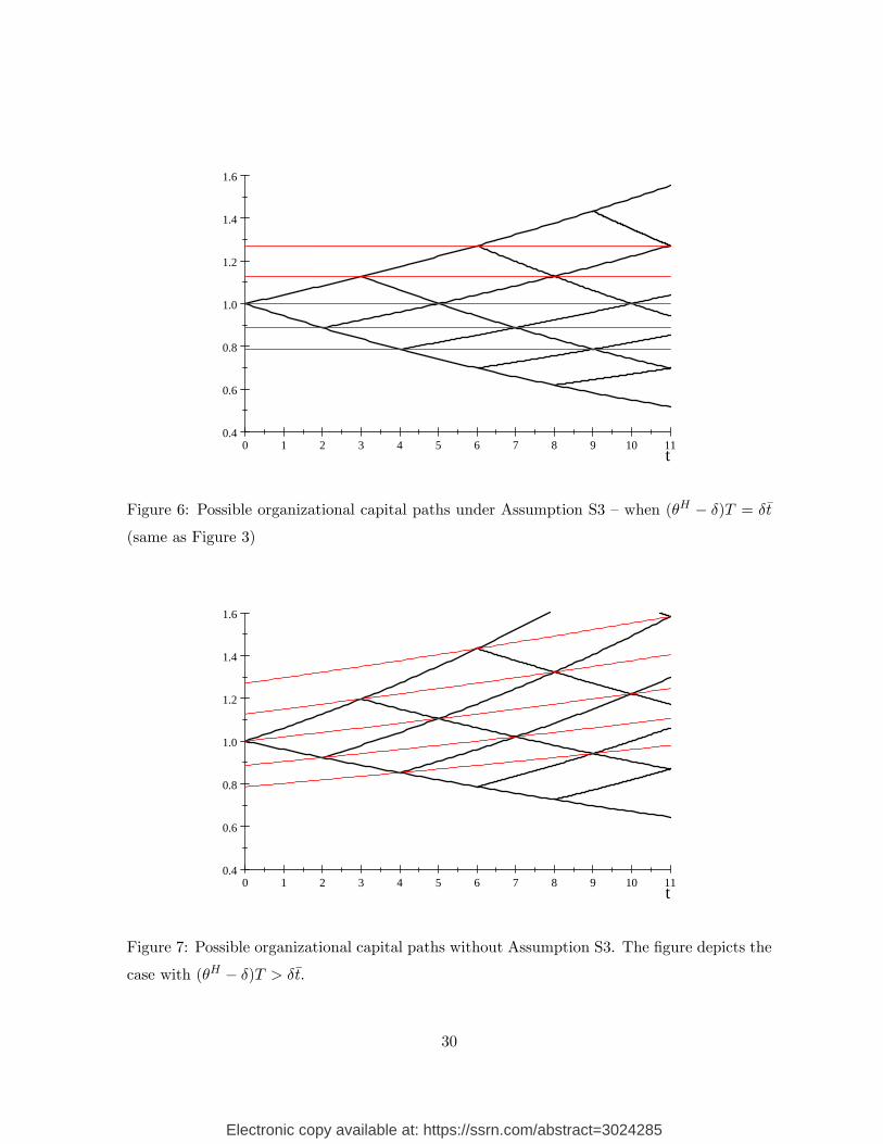
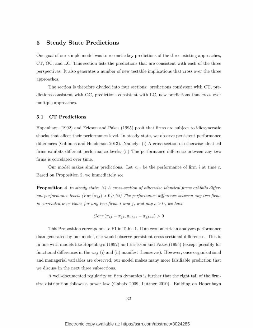
bad CEO, as depicted in Figure 6. We now remove this non-generic condition and allow the

effect of a good CEO to be greater or smaller than that of a bad CEO. If, for instance, a good

CEO has a larger absolute effect, then we have a situation as shown in Figure 7.

The red lines in Figure 7 can be called neutral transition paths. Assume without loss of

generality that at t = 0, one of the neutral transition paths goes through Ω0 = π0 = 1. Then,

that path is defined by

π0 (t) = e(θH−δ)T−δt

T+tt

and all other transition paths are defined by Ωj (t) = π0 (t) (1 + ∆′)j where j is an integer and

1 + ∆′ = e(θH−δ)T−

((θH−δ)T−δt

T+t

)T

= eθH tTT+t

All firms which experience a CEO transition at time t have organizational capital Ω = Ωj (t)

for some j ∈ Z. Consider therefore the set of (time-dependent) CEO transition organizationalcapital levels

Π(t) =

Ω : ∃j ∈ N such that Ω = Ωj(t) ≡ π0 (t) (1 + ∆′)j

(7)

We are interested in characterizing a steady state economy with a balanced growth path,

that is a steady state where all variables grow at a constant rate.17 In the context of our model,

this requires that the performance level π0 at which firms exit is growing at a constant rate as

well. It is immediate to see the following:

Proposition 3 Suppose g(j) is the steady state measure of firms with organizational capital

Ωj ∈ Π for an environment defined by(p, θH , δ, T, t

)with (θH − δ)T = δt. Then at time t,

16Formally, if firms are born at organizational capital level Ωk only and the steady state distribution is

unimodal, then the modal organizational capital level cannot be greater than Ωk. Indeed, suppose it is. Then

we must have that f∗(k + 1

)> f∗

(k)> f∗

(k − 1

). But is easy to see that this also implies that f∗

(k + 2

)>

f∗(k + 1

)> f∗

(k)and so on, because the difference equation is then always the same for k ≥ k + 2.

17 In neoclassical growth theory, a balanced growth path refers to a steady state where both output and capital

grow at a constant rate.

29


0 1 2 3 4 5 6 7 8 9 10 110.4

0.6

0.8

1.0

1.2

1.4

1.6

t

Figure 6: Possible organizational capital paths under Assumption S3 —when (θH − δ)T = δt

(same as Figure 3)

0 1 2 3 4 5 6 7 8 9 10 110.4

0.6

0.8

1.0

1.2

1.4

1.6

t

Figure 7: Possible organizational capital paths without Assumption S3. The figure depicts the

case with (θH − δ)T > δt.

30


g(j) is also the steady state measure of firms with organizational capital Ωj(t) ∈ Π(t) for any

environment defined by(p, θ′H , δ′, T ′, t′

)where firms die whenever they reach π0 (t).18 In this

steady state:

• All organizational capital levels Ωj(t) ∈ Π(t) as well as total output are increasing at a

constant rate.

• Better ex post governance (smaller t) increases the average CEO behavior/type and

growth rate of organizational capital.

• In the limit as ex post agency problems disappear (t goes to zero), firm heterogeneity

vanishes as well. Conversely, differences between any two performance levels j and j′ are

increasing in ex post agency problems (t).


Proposition 3 characterizes a steady state with a balanced growth path. All organiza-

tional capital levels j = 0, 1, 2, ..., including organizational capital level Ω0 = π0 at which firms

exit, are growing at a constant rate, given by

(θH − δ)T − δtT + t

An appealing feature of this steady state is that firm heterogeneity disappears as ex post

governance becomes perfect. In the limit where bad CEOs are fired immediately (t goes to 0),

the difference between any two organizational capital levels j and l > j goes to zero as well.

Formally, we have that the ratio of two subsequent organizational capital levels is given by

Ωj+1 (t)

Ωj(t)= 1 + ∆′ = eθ

H tTT+t

which is decreasing in t and equals 1 in the limit as t goes to 0. The growth rate of the economy

then converges to θH − δ, which is exactly the growth rate of the organizational capital of afirm led by a good CEO.

A final comparative static discussed in Proposition 3 regards the impact of better ex

post governance (a lower t) on the average CEO type and average CEO behavior. While the

fraction of newly appointed CEOs who are mediocre and behave badly is constant, better ex

post governance (a lower tenure for mediocre CEOs) increases the average CEO type.

18Maintaining the assumption that θ′H and δ′ are consistent with the conditions in Proposition 1.

31


5 Steady State Predictions

One goal of our simple model was to reconcile key predictions of the three existing approaches,

CT, OC, and LC. This section lists the predictions that are consistent with each of the three

perspectives. It also generates a number of new testable implications that cross over the three

approaches.

The section is therefore divided into four sections: predictions consistent with CT, pre-

dictions consistent with OC, predictions consistent with LC, new predictions that cross over

multiple approaches.

5.1 CT Predictions

Hopenhayn (1992) and Ericson and Pakes (1995) posit that firms are subject to idiosyncratic

shocks that affect their performance level. In steady state, we observe persistent performance

differences (Gibbons and Henderson 2013). Namely: (i) A cross-section of otherwise identical

firms exhibits different performance levels; (ii) The performance difference between any two

firms is correlated over time.

Our model makes similar predictions. Let πi,t be the performance of firm i at time t.

Based on Proposition 2, we immediately see

Proposition 4 In steady state: (i) A cross-section of otherwise identical firms exhibits differ-

ent performance levels (V ar (πi,t) > 0); (ii) The performance difference between any two firms

is correlated over time: for any two firms i and j, and any s > 0, we have

Corr (πi,t − πj,t, πi,t+s − πj,t+s) > 0

This Proposition corresponds to F1 in Table 1. If an econometrican analyzes performance

data generated by our model, she would observe persistent cross-sectional differences. This is

in line with models like Hopenhayn (1992) and Erickson and Pakes (1995) (except possibly for

functional differences in the way (i) and (ii) manifest themseves). However, once organizational

and managerial variables are observed, our model makes many more falsifiable prediction that

we discuss in the next three subsections.

A well-documented regularity on firm dynamics is further that the right tail of the firm-

size distribution follows a power law (Gabaix 2009, Luttner 2010). Building on Hopenhayn

32


(1992) and Gabaix (1999), Luttner (2007) shows how —given the appropriate assumptions on

the entry and exit process—models of firm dynamics with idiosyncratic shocks can generate

such power laws. Similarly, as shown in Proposition 1, our model predicts that the right tail of

the distribution of organizational capital follows a power law. This corresponds to F2 in Table

1.

5.2 OC Predictions

Suppose now that the econometrician observes performance as well as organizational variables.

The leading example is Bloom and Van Reenen (2007), where the form of organizational capital

observed is the quality of management practices. They document how, after controlling for

all observables, (changes in) the quality of management practices explains (changes in) firm

performance. Moreover, the quality of management practices is correlated with corporate

governance and the availability of managerial human capital.

These predictions are consistent with the relation between performance π and organiza-

tional capital Ω in our model. Again, take a steady state with a mass of otherwise identical

firms. In our model, the quality of governance depends on how well bad CEOs are screened

out before they are hired, as captured by p, and how quickly bad CEOs are fired after they

are hired, as captured by t = min K,R, where R is the firm’s monitoring technology and

K = ln(1 + b

)/θH . K is increasing in the ability of the CEO to create short term performance

(the lower is b, the faster bad CEOs are fired), and decreasing in a measure of managerial

human capital, θH . Note that also p can be seen as a measure of the supply of managerial

human capital (extensive margin).

Define average performance growth, E (∆π) , as the average (instantaneous) growth of

a randomly selected firm. From Proposition 2, we see:

Proposition 5 In steady state:

(i) In a cross-section of firms, performance and organizational capital are positively

correlated: Corr (πi,t,Ωi,t) > 0.

(ii) In a cross-section of firms, changes in performance are positively correlated with

changes in organizational capital:19

Corr (πi,t+s − πi,t,Ωi,t+s − Ωi,t) ≥ 0

19 If s > t, the correlation is strictly positive.

33


(iii) Average performance growth is increasing in the quality of ex ante and ex post

corporate governance and in the availability of managerial talent:

d

dpE (∆π) > 0,

d

dtE (∆π) < 0,

d

dθHE (∆π) > 0.


In steady state, ex ante identical firms have different levels of organizational capital, and

this affects their performance. The heterogeneity is due to different leadership styles in the

past. The same is true in terms of changes: firms whose last CEO was a good type experience

a growth in both their organizational capital and their performance.

Note that in the model the effect of organizational capital on performance is causal.

So, if an external intervention such as the one in Bloom et al (2013) were to increase Ωi,t, it

would also increase performance πi,t+s. Of course, the benefit of the model is that it explains

where the heterogeneity in organizational capital comes from and it links it to another set of

observables, as discussed below.

Proposition 5 corresponds to F4, F5, and F6 of Table 1.

5.3 LC Predictions

The LC approach has studied the effect of CEO variables on firm performance (Bertrand and

Schoar 2003, Bennedsen et al 2007, Kaplan et al 2012, Bandiera et al 2016). The CEO variables

considered include the identity, the characteristics, and the behavior of the CEO.

The next section, where CEOs will be allowed to work at multiple firms and salaries

are endogenous, will generate even more testable predictions on career trajectories and com-

pensation patterns. However, for now, let us focus on the implications of the stylized model

considered so far.

Consistent with the core of those observed patterns, our model predicts a connection

between CEO variables and performance. In the equilibrium described in Proposition 1, good

CEOs behave differently, produce more organizational capital, generate better performance,

and stay longer on the job. This in turn leads to a number of cross-sectional patterns:

Proposition 6 (a) In steady state, firm i’s current performance level πi,t is higher when past

CEOs: (i) Chose the organization-building behavior rather than the short-term profit boost

34


(xi,t−s = 1 not 0); (ii) Were of the high type rather than the low type (θi,t−s = θH not θL);

(iii) Had longer on-the job tenure (T not t).

(b) In steady state, in a cross-section of firms, better governance (lower b or lower R)

weakly increases the average behavior and type of the CEO, the tenure variance among CEOs,

and average performance.

Note that predictions (a)(i) and (a)(ii) hold also in a probabilistic sense. If certain cate-

gories of CEOs are more likely to be high types and behave well, the firms run by those CEOs

will in general have better performance and higher organizational capital. This rationalizes

the findings of Bennedsen et al (2007) that family and professional CEOs impact long term

performance differently.20 Finding (a)(iii) is to the best of our knowledge untested but it is

an immediate implication of a model where bad CEOs are more likely to be dismissed early.

Finding (b) is consistent with classic findings of the literature on international differences in

governance (see for instance the influential survey by Shleifer and Vishny 1997). These findings

correspond to F8 and F9 of Table 1.

5.4 Predictions Linking OC and LC

As mentioned in the introduction, the OC and LC approaches have mostly operated in a

separate manner. Our model suggests a number of testable implications involving OC variables

and LC variables. CEOs play a part in growing or destroying organizational capital, which

in turn determines performance. So our model predicts a lagged effect of CEO variables on

organizational capital. It is immediate to see that:

Proposition 7 (a) In steady state, the rate of growth of organizational capital Ωi,t is greater

when the current CEO: (i) Chooses the organization-building behavior rather than the short-

term proft boost (xi,t = 1 not 0); (ii) Is of the high type rather than the low type (θi,t = θH not

θL); (iii) Has longer on-the job tenure (T not t).

(b) Firm i’s current organizational capital Ωi,t is higher when past CEOs: (i) Chose the

organization-building behavior rather than the short-term proft boost (xi,t−s = 1 not 0); (ii)

Were of the high type rather than the low type (θi,t−s = θH not θL); (iii) Had longer on-the-job

tenure (T not t).20Our model does not capture the feature that family CEOs are often diffi cult to dismiss. The result would

hold a fortiori.

35


(c) Controling for current organizational capital Ωi,t, past CEO variables have no pre-

dictive value on current firm performance πit.

Organizational capital is a stock, while CEO behavior is a flow that influences the growth

of the stock. Part (a) is an immediate consequence of this: organizational capital grows faster

when at least one of the folllowing is true: the CEO behaves better, is a higher type, or has been

there for longer (meaning that his type is more likely to be high). Part (b) is the cumulative

correspondent of part (a): the current level of organizational capital is predicted by the type,

behavior, and tenure of past CEOs. For instance, a firm that has experienced a sequence of

short-lived CEOs is predicted to have a lower organizational capital. The first two parts of the

proposition correspond to F8 of Table 1.

Part (c), which corresponds to F11 of Table 1, helps distinguish the present model from

other stories that give the CEO a productive role. It is reasonable to expect Part (c) to be

falsified in reality. For instance, a charismatic CEO may have a direct motivating effect on

employees that does not go through the growth of organizational capital. Such a model would

create a direct link between CEO type/behavior and performance that would violate Part (c).

In practice it would be interesting to see how much of the CEO effect operates through

organizational capital, as postulated in our model, as opposed to other avenues. Part (c)

suggests a possible way of disentangling these two sets of channels.

6 Model with Endogenous Wages and CEO Quality

So far we have assumed that CEOs only work once. What happens if a CEO can “prove

herself”in one firm and then go to another firm? Which firms will hire better CEOs?

In this section, we first show a general result: if multiple CEO types are available and

higher types are scarce, better CEOs will be hired by firms that already have more organiza-

tional capital.

We then apply this general result to a situation where CEOs can take a succession of

jobs. In equilibrium, rookie CEOs are hired by low-performance firms. If they succeed, they

move on to better firms. The salary differential between new and proven CEOs is determined

in equilibrium.

36


6.1 The Marginal Value of CEO Quality

Reconsider our baseline model but assume that there are multiple categories of prospective

CEOs. CEOs in category j have a pj probability of being type θH and a 1− pj probability ofbeing type θL. CEO compensation is endogenous. Assume that there is an unlimited number

of CEOs of the lower category (j = 1), but the total number of CEOs of higher categories

is smaller than the total number of firms, so that CEO quality will have to be rationed. In

equilibrium all CEOs in category j earn the same instantaneous wage wj (we are maintaining

the hypothesis that the only possible form of compensation is a constant per period wage).

Which firms will pay to get the most promising CEOs?

We assume that the cash flow boost b is not only bounded above by b, but it also does

not allow the CEO to reach a performance level that is greater than that of a high-quality

CEO who chooses x = 1.21 Without this additional assumption, a highly impatient firm might

ask its CEO to engage in short term profit boosting. Alternatively, one could assume that b is

not profit boosting, but covert borrowing: unbeknown to the board, the CEO borrows funds

on behalf of the firm at instantaneous rate ρ that must be repaid by the firm when the CEO

is fired. The result below holds a fortiori in the alternative scenario.

For the rest, the model is unchanged. We can show:

Proposition 8 Consider a CEO with p′ and a CEO with p′′ > p′. Let Ω′ and Ω′′ denote

the organizational capital levels of the firms employing the two CEOs respectively. If firms are

suffi ciently impatient (ρ is suffi ciently high), in steady state Ω′ ≤ Ω′′.

Proof. See Appendix

Proposition 8 says that more promising CEOs must be hired by firms with higher orga-

nizational capital. A CEO with a higher p is more likely to protect the firm’s organizational

capital —something that is more useful when the size of the organizational capital is larger.

The key assumption is that the effect of CEO behavior/type on organizational capital is mul-

tiplicative:

Ωt = (θx− δ) Ωt,

To reverse this effect, one must assume that

Ωt = θxz (Ωt)− δΩt,

21Formally, if t is the time when the CEO was hired and s is her tenure, bs ∈[0,min

(b, e(θ

H−δ)s)].

37


where z (·) is a decreasing function. In that case, firms with lower organizational capital mayhire more promising CEOs.

The requirement that ρ is suffi ciently high is mainly technical and derives from the

inability to characterize the value function of this problem.

Proposition 8 is related in spirit to results on assortative matching between CEOs and

firm size (Tervio (2008) and Gabaix and Landier (2008)). There, more capable CEOs are

matched with larger firms. Here, CEOs who are more likely to be good are matched with

firms with a higher organizational capital. The connection would become direct if we used the

production function in (2).

Of course, the fact that more expensive CEOs are more likely to be good types does

not eliminate the stochastic element that underpins our organizational capital process. Even

an expensive CEO may turn out to be bad and destroy organizational capital. The following

section explores such dynamics.

6.2 Equilibrium with Proven CEO Quality

Consider now the endogenous allocation of CEO talent. As before, there are two types of CEOs,

good and bad, and CEOs that are revealed to be bad can be fired at any time. We maintain

S1-S3 above so that a bad CEO exactly undoes the effect of a good CEO on organizational

capital. But rather than retiring after a period of time T, a good CEO may move to a different

firm.22 We assume that the type of a CEO is only partially persistent. A CEO with a low

type always remains low. A CEO with a high type becomes a low type with probability κ at

the end of a contract term T .

There are then three categories of CEOs. A new CEO denote a CEO who has never

worked. We assume that there is never any scarcity of potential new CEOs and a share pL of

them is of the high type. The type of new CEOs is unobservable. Let a successful CEO denote

a CEO which has already been hired at least once and completed a period of time T (which

is now the “standard” contract duration). We denote by pH ≡ 1 − κ the probability that asuccessful CEO remains a high type. We assume that the type persistence is suffi ciently large

so that pH > pL. Finally, let a failed CEO denote a CEO who was hired and then fired.

22For simplicity, we assume that CEOs can only move to a different firm after their contract term T.Without

loss of generality, their contract may also be renewed at the same firm.

38


We consider a competitive market for managerial talent, where firms offer CEOs a wage

w based on their performance. The wage w is fixed for the duration of the contract (or until

the CEO is fired). Since there is no scarcity of new CEO’s, the wage of new CEO’s is set equal

to their reservation value, which we normalize to 0. For the same reason, no firm ever hires a

failed CEO. Consider now the successful CEOs. In steady state, the fraction of (previously)

successful CEOs among all CEO hires is given by

µ = pL(1− µ) + pHµ =pL

1− pH + pL.

In line with the intuition developed in Proposition 8, successful CEOs will receive a positive

wage w > 0 and they will be hired by the share µ of most productive firms. In particular, we

obtain the following result, proven for the case where ρ is suffi ciently large (firms are suffi ciently

myopic):

Proposition 9 Assume ρ is suffi ciently large. In steady state, there exists a cutoff π such

that:

• Firms with productivity πt > π hire only successful CEOs and pay a wage differential

w > 0.

• Firms with πt < π hire only new CEOs.

• No firm hires failed CEOs.

• Firms at πt = π are indifferent between hiring a new CEO or a (more expensive) suc-

cessful CEO.

• Each firm’s organizational capital at CEO transition times follows a Markov chain: if thefirm is at level Ωj, the probability of going up (down) one level is given by pi ((1− pi)),where

pi

= pL if Ωj < π

∈ [pL, pH ] if Ωj = π

= pH if Ωj > π

Proof. We prove by contradiction. Let q = (ql)l∈N be the steady state hiring profile where

ql ∈ pH , pL denotes the type of manager hired at organizational capital level Ωj ∈ Π. Assume

39


that our proposition does not hold. Then there must exists an m such that q(m) = pH but

q(m+ 1) = pL. But by Proposition 8, this is impossible.

When Ωk = π, the firm is indifferent over whether to hire a successful CEO or a new

one. This creates (local) equilibrium multiplicity, which is allowed for in the statement of

the proposition. For performance levels above and below π, the stochastic process is uniquely

defined.

6.3 Implications of the Endogenous Wage Model

Section 5 discussed the testable implications of the baseline model where CEOs can only work

for one period. Let us now examine the additional predictions we can make when CEOs work

for multiple periods and wages are endogenous.

In the equilibrium in Proposition 9, CEO careers display certain patterns. Bad CEOs

are employed only once: after damaging the organizational capital of one firm, they become

unemployable. Good CEOs are employed repeatedly and receive a compensation premium

until they underperform. Firms with higher organizational capital hire better CEOs.


(i) Firms with better performance and higher organizational capital employ CEOs of a

better type (on average), with better behavior (on average), who are paid more.

(ii) The current employment status and compensation of a CEO depends on the change

in performance and organizational capital of its previous firm.

(iii) A fixed-effect regression on data generated by this model returns significant individual

coeffi cients but underestimates the true effect of individual CEOs on performance.


Prediction (i) (F3 in Table 1) relates to an influential prediction of the CT literature:

larger firms should hire better CEOs on average (Tervio (2008) and Gabaix and Landier

(2008)). It also has a potential connection with the findings by Bender et al (2016) that

firms with better management performance also hire workers —especially highest paid workers

—with higher human capital.

Prediction (ii) (F12 in table 1) relates the career path of CEOs to their effect on previous

firms they worked for. Past employers of CEOs who currently command higher wages and work

40


for more productive firms have experienced unusually strong growth in both performance and

organizational capital.

Prediction (iii) (F13 in table 1) relates to the estimation of CEO fixed effects developed

by Bertrand and Schoar (2003). Consider an econometrician who observes the last N periods

of a random sample of firms and estimates fixed effects for firms and CEOs. As firms with

high organizational capital hire better CEOs on average, part of the CEO fixed effect will be

attributed to the firm, thus underestimating the true causal effect of CEO on performance.

The presence of this selection bias means that the CEO fixed effect estimated by Bertrand and

Schoar (2003) is a lower bound to the true fixed effect.

7 Conclusions

This paper began by noting that economists have studied the effect of management on firm

performance from three distinct perspectives: CT, OC, and LC. The goal of the paper was

to develop a parsimonious model that can reconcile key patterns predicted or observed by the

three perspectives. The main novel ingredient of the model was organizational capital, a set

of productive assets that can only be produced with the direct input of the firm’s leadership

and is subject to an agency problem. Besides yielding predictions that are consistent with the

three perspectives, the model generates novel predictions that combine OC and LC variables.

References

Baker, George, Robert Gibbons and Kevin J. Murphy (2002). Relational Contracts and the

Theory of the Firm. Quarterly Journal of Economics. 117(1), pp. 39-84.

Bandiera, Oriana, Stephen Hansen, Andrea Prat, and Raffaella Sadun (2016). CEO Behavior

and Firm Performance. Journal of Political Economy, forthcoming.

Bebchuk, Lucian (2009). Pay Without Performance: The Unfulfilled Promise of Executive

Compensation. Harvard University Press, Cambridge, Massachusets.

Bender, Stefan, Nicholas Bloom, David Card, John Van Reenen, and Stefanie Wolter (2018).

Management Practices, Workforce Selection and Productivity. Journal of Labor Eco-

nomics 36(S1), pp. S371-S409.

41


Bennedsen, Morten, Kasper Meisner Nielsen, Francisco Pérez-González, and Daniel Wolfen-

zon (2007). Inside the Family Firm: The Role of Families in Succession Decisions and

Performance. Quarterly Journal of Economics 122(2), pp. 647-691.

Bertrand, Marianne (2009). CEO’s. Annual review of Economics 1(1), pp. 121-150.

Bertrand, Marianne and Antoinette Schoar (2003). Managing with Style: The Effect of

Managers on Firm Policies. Quarterly Journal of Economics 118(4), pp. 1169-1208.

Besley, Timothy and Torsten Persson (2018). Organizational Dynamics: Culture, Design,

and Performance. Working paper, London School of Economics.

Bloom, N., Brynjolfsson, E., Foster, L., Jarmin, R., Patnaik, M., Saporta-Eksten, I., and

Van Reenen, J. (2019). What Drives Differences in Management Practices? American

Economic Review 109(5), pp. 1648-83.

Bloom, Nicholas, Benn Eifert, Aprajit Mahajan, David McKenzie, and John Roberts (2013).

"Does Management Matter? Evidence from India." Quarterly Journal of Economics

128(1), pp. 1-51.

Bloom, Nicholas, Raffaella Sadun, and John Van Reenen (2016). Management as a Technol-

ogy?. NBER Working Paper 22327. April 2016.

Bloom, Nicholas, and John Van Reenen (2007). Measuring and Explaining Management

Practices Across Firms and Countries. Quarterly Journal of Economics 122(4), pp.

1351-1408.

Board, Simon, Moritz Meyer-ter-Vehn, and Tomasz Sadzik. Recruiting Talent. (2016). Work-

ing paper.

Bolton, Patrick, Markus K. Brunnermeier, and Laura Veldkamp (2012). Leadership, Coordi-

nation, and Corporate Culture. Review of Economic Studies 80(2), pp. 512-537.

Chassang, Sylvain (2010) Building routines: Learning, Cooperation, and the Dynamics of

Incomplete Relational Contracts. American Economic Review 100(1), pp. 448-465.

Cheng, Sui Sun (2003). Partial Difference Equations. London: CRC Press.

42


Drucker, Peter (1967), The Effective Executive. New York: Harper & Row

Ellison, Glen and Richard Holden (2014). A Theory of Rule Development. Journal of Law,

Economics and Organization 30(4), pp. 649-682.

Ericson, Richard, and Ariel Pakes (1995). Markov-perfect Industry Dynamics: A Framework

for Empirical Work. Review of Economic Studies 62(1), pp. 53-82.

Gabaix, Xavier, and Augustin Landier (2008). Why Has CEO Pay Increased so Much?

Quarterly Journal of Economics 123(1), pp. 49-100.

Garicano, Luis, and Esteban Rossi-Hansberg (2006). Organization and Inequality in a Knowl-

edge Economy. Quarterly Journal of Economics 121(4), pp. 1383—1435.

Gibbons, Robert, and Rebecca Henderson (2013). What Do Managers Do? Exploring Per-

sistent Performance Differences among Seemingly Similar Enterprises. Handbook of Or-

ganizational Economics, eds. Robert Gibbons and John Roberts, Princeton University

Press, pp. 680-731.

Gibbons, Robert, Marco Li Calzi and MassimoWarglien (2017). Shared Frames and Economic

Interaction: How Categorizations Can Shape Interactions (and How Leaders Can Shape

Categorizations). Working paper, MIT.

Graham, John R., Campbell R. Harvey, Jillian A. Popadak, and Shivaram Rajgopal (2016).

Corporate Culture: Evidence from the Field. Working paper.

Halac, Marina, and Andrea Prat (2016). Managerial Attention and Worker Performance.

American Economic Review 106(10), pp. 3104-3132.

Hennes, Karen M., Andrew J. Leone, and Brian P. Miller (2008). The Importance of Distin-

guishing Errors from Irregularities in Restatement Research: The Case of Restatements

and CEO/CFO Turnover. The Accounting Review 83(6), pp. 1487-1519.

Hermalin, Benjamin E (2013). Leadership and Corporate Culture. Handbook of Organiza-

tional Economics, eds. Robert Gibbons and John Roberts, Princeton University Press,

pp. 432-478.

43


Hoffman, Mitchell and Steven Tadelis (2017). How Do Managers Matter? Evidence from

Performance Metrics and Employee Surveys in a Firm. Working paper, University of

Toronto.

Hopenhayn, Hugo A. (1992) Entry, Exit, and Firm Dynamics in Long Run Equilibrium.

Econometrica 60(5), pp. 1127-1150.

Ichniowski, Casey, Kathryn Shaw, and Giovanna Prennushi (1997). The Effects of Human

Resource Management Practices on Productivity: A Study of Steel Finishing Lines.

American Economic Review pp. 291-313.

Jensen, Michael C., and William H. Meckling (1976). Theory of the Firm: Managerial Be-

havior, Agency Costs and Ownership Structure. Journal of Financial Economics 3(4),

pp. 305-360.

Johnson, W.Bruce, Robert P. Magee, Nandu J.Nagarajan, Harry A.Newman (1985). An

Analysis of the Stock Price Reaction to Sudden Executive Deaths: Implications for the

Managerial Labor Market. Journal of Accounting and Economics. 7(1—3), pp. 151-174.

Jones, Benjamin F., and Benjamin A. Olken (2005). Do Leaders Matter? National Leadership

and Growth since World War II. The Quarterly Journal of Economics 120(3), pp. 835-

864.

Kaplan, Steven N., Mark M. Klebanov, and Morten Sorensen (2012). Which CEO Charac-

teristics and Abilities Matter? The Journal of Finance 67(3), pp. 973-1007.

Kotter, John P. (2001). What Leaders Really Do. Harvard Business Review 79(5), pp. 62-70.

Lazear, Edward P, Kathryn L. Shaw, and Christopher T. Stanton (2015). The Value of

Bosses. Journal of Labor Economics 33(4), pp. 823—861.

Li, Jin, Niko Matouschek and Michael Powell (2017). Power Dynamics in Organizations.

American Economic Journal: Microeconomics 9(1), pp. 217-41.

Lucas Jr, Robert E. (1978). On the Size Distribution of Business Firms. The Bell Journal of

Economics, pp. 508-523.

44


Luttmer, Erzo G.J. (2010). Models of Growth and Firm Heterogeneity. Annu. Rev. Econ.

2(1), pp. 547-576.

Milgrom, Paul, and John Roberts (1995). Complementarities and Fit Strategy, Structure, and

Organizational Change in Manufacturing. Journal of accounting and economics 19(2),

pp. 179-208.

Powell, Michael (2019). Productivity and Credibility in Industry Equilibrium. Rand Journal

of Economics 50(1), pp. 121-146.

Prescott, Edward C., and Michael Visscher (1980). Organization Capital. Journal of Political

Economy 88(3), pp. 446-461.

Rahmandad, Hazhir, Nelson Repenning, and Rebecca Henderson (2018). Making the Num-

bers? ’Short Termism’and the Puzzle of Only Occasional Disaster. Management Science

64(3), pp. 983-1476.

Sannikov, Yuliy (2007). Games with Imperfectly Observable Actions in Continuous Time.

Econometrica 75(5), pp. 1285-1329.

Schein, Edgar (2010). Organizational Culture and Leadership. John Wiley & Sons.

Shleifer, Andrei and Robert W. Vishny (1997). A Survey of Corporate Governance. Journal

of Finance. 52(2), pp. 737—783.

Simons, Robert (1994a). Levers of Control: How Managers Use Innovative Control Systems

to Drive Strategic Renewal. Harvard Business Press, Cambridge.

Simons, Robert (1994b). How New Top Managers Use Control Systems as Levers of Strategic

Renewal. Strategic Management Journal, 15: 169-189.

Stein, Jeremy C.(1989) Effi cient Capital Markets, Ineffi cient Firms: A Model of Myopic

Corporate Behavior. The Quarterly Journal of Economics 104(4), pp. 655-669.

Syverson, Chad (2004). Product Substitutability and Productivity Dispersion. Review of

Economics and Statistics, 86(2), pp. 534-50.

Syverson, Chad (2011) What Determines Productivity? Journal of Economic Literature

49(2), pp. 326-365.

45


Teece, David J. Gary Pisano, and Amy Shuen (1997). Dynamic Capabilities and Strategic

Management. Strategic Management Journal 18(7), pp. 509—533

Terviö, Marko (2008). The difference that CEOs make: An Assignment Model Approach.

The American Economic Review, 98(3), pp. 642-668.

Tirole, Jean (2010). The Theory of Corporate Finance. Princeton University Press.

Van den Steen, Eric J. (2005). Organizational Beliefs and Managerial Vision. Journal of Law,

Economics & Organization 21(1), pp. 256—283.

Van den Steen, Eric J. (2018). Strategy and the Strategist: How it Matters Who Develops

the Strategy. Management Science 64(10), pp. 4533—4551.

Von Thadden, Ernst-Ludwig (1995). Long-term Contracts, Short-term Investment and Mon-

itoring. Review of Economic Studies 62(4), pp. 557-575.

46


Appendix I: Proof of Proposition 2

Proposition 2: The distribution of firms over transition organizational capital levels Ωj ∈ Π,

g(j), is given by

g(2k) = f∗ (k) ≡ 4B ∗ k(

p

1− p

)kfor j = 2k with k ∈ N, and

g(2k − 1) =√

1 + γ∗ [pf∗ (k − 1) + (1− p)f∗(k)]

for j = 2k − 1, with G∗ = Σjg(j).

For the proof, we proceed in five steps.

Part 1: Solution of the difference equation In steady state, f (·) must satisfy thedifference equation (5),

f (k) = (1 + γ)(p2f (k − 1) + 2 (1− p) pf (k) + (1− p)2 f (k + 1)

), (8)

with the following boundary conditions:

f(0) = 0 and f(1) =B

(1 + γ)(1− p)2

For every value of γ, standard techniques show that the difference equation (5) has at

most one solution with non-negative values of f (·) as follows:

f (k) =Ak −Dk

C,

where

A = A(γ) =1

2

(1− 2p (1 + γ) + 2p2 (1 + γ)

(1− p)2 (1 + γ)+

√1− 4p (1 + γ) + 4p2 (1 + γ)

(1− p)4 (1 + γ)2

);

D = D(γ) =1

2

(1− 2p (1 + γ) + 2p2 (1 + γ)

(1− p)2 (1 + γ)−√

1− 4p (1 + γ) + 4p2 (1 + γ)

(1− p)4 (1 + γ)2

);

C = C(γ) =1

B(1 + γ) (1− p)2

√1− 4p (1 + γ) + 4p2 (1 + γ)

(1− p)4 (1 + γ)2

Let

γ∗ ≡ (1− 2p)2

1− (1− 2p)2

47


Consider the term under the three square roots that appears in the expressions of A, D, and

C. When γ > γ∗, the term is negative, in which case it can be shown that f (k) is strictly

negative for certain values of k.23 When γ → γ∗, the expression above tends to:

f∗ (k) = B

(1− (1− 2p)2

(1− p)2

)k

(p

1− p

)k−1

= 4B ∗ k(

p

1− p

)kPart 2: Impossibility of γ > γ∗ We first rule out steady states with γ > γ∗. Intuitively,

there cannot be a steady state with an excessively large γ because the distribution would keep

shifting to the right. This impossibility is shown by proving that in a steady state with γ > γ∗

there must be negative values of f (k).

Lemma 3 If γ > γ∗ there exists k > 1 such that f (k) < 0.

Proof. Consider the term under the three square roots that appears in the expressions of A,

D, and C. When γ > γ∗, the term is negative and A, B, and C are complex numbers.

Note that we can rewrite

f (k) = H

(a+√b)k−(a−√b)k

√b

,

where

H =B

2k

(1

(1− p)2 (1 + γ)

)ka = 1− 2p (1 + γ) + 2p2 (1 + γ)

b = 1− 4p (1 + γ) + 4p2 (1 + γ)

Note that b < 0 when γ > γ∗ and√b is a complex number.

As H is a positive real number, the analysis will focus on the sign of:

S (k) ≡

(a+√b)k−(a−√b)k

√b

23The fact that the value under the square root is negative is not a problem per se because all terms with an

even power drop out. However, for k large enough, f (k) < 0.

A feasible solution for f (k) does not exist when γ is too high, because a very high birth rate leads to explosive

growth in the number of firms.

48


We begin by showing that, although√b is a complex number, S (k) is a real number for

every k. To see this note that:

S (k) =ak − ak√

b+ 2δ1

ak−1√b√

b+ δ2

ak−2(√

b)2− ak−2

(√b)2

√b

+ 2δ3

ak−3(√

b)3

√b

+ · · ·

where

δj =k!

j! (k − j)! .

Therefore

S (k) = 2(δ1a

k−1 + δ3ak−3b+ δ5a

k−5b2 + δ7ak−7b3 + · · ·

),

which is a real number.

If a < 0, we have that S (2) = δ1a < 0, and the lemma is proven for k = 2.If a = 0,

S (k) = 0 for all k, which is clearly impossible. Therefore, from now on, assume that a > 0

(note that with γ = γ∗, we have a = 1/2, so the case is relevant).

Rewrite the summation as

1

2S (k) = δ3a

k−3

(δ1

δ3a2 + b

)+ δ7a

k−7b2(δ5

δ7a2 + b

)+ · · ·

=

k∑j=0

δ4j+3ak−3−4jb2j

(δ1+4j

δ3+4ja2 + b

)Note that for i ≥ 3

δi−2

δi=

k!(i−2)!(k−i+2)!

k!i!(k−i)!

=(i− 2)! (i− 1) i (k − i)!

(i− 2)! (k − i+ 2) (k − i+ 1) (k − i)! =(i− 1) i

(k − i+ 2) (k − i+ 1)

Thus,

1

2S (k) =

k∑j=0


((3 + 4j − 1) (3 + 4j)

(k − 3− 4j + 2) (k − 3− 4j + 1)a2 + b

)Take any k that is the square of an integer h. Consider a series that comprises the first

h elements of S (k):

1

2S (h) =

h∑j=0


((3 + 4j − 1) (3 + 4j)

(k − 3− 4j + 2) (k − 3− 4j + 1)a2 + b

)

=h∑j=0

δ4j+3ah2−3−4jb2j

((3 + 4j − 1) (3 + 4j)

(h2 − 3− 4j + 2) (h2 − 3− 4j + 1)a2 + b

)

49


By construction

limh→∞

S (h) = limk→∞

S (k)

Note that, with h is suffi ciently large,

(3 + 4j − 1) (3 + 4j)

(h2 − 3− 4j + 2) (h2 − 3− 4j + 1)≤ (3 + 4h− 1) (3 + 4h)

(h2 − 3− 4h+ 2) (h2 − 3− 4h+ 1)≤ 16

h2,

and hence1

2S (h) ≤

(16

h2a2 + b

) h∑j=0

δ4j+3ah2−3−4jb2j .

As a and b2 are positive, for h suffi ciently large the value of the summation is positive.

Therefore:

limh→∞

1

2S (h) = b lim

h→∞

h∑j=0

δ4j+3ah2−3−4jb2j < 0,

which completes the proof of the lemma.

Part 3: Impossibility of γ < γ∗ We now show that γ < γ∗ is not consistent with the

condition that the steady state is reachable from below.

Consider the N -level version of our problem where we impose the boundary condition

ft(k) = 0 for k > N with N a finite positive integer. In this finite version of our problem,

organizational capital is bounded above by ΩN .

Let us denote by fN,t(k) the mass of firms with organizational capital level 2k at time

t in the finite N -level version of our problem. If a steady state of this finite version exists

where fN,t(k) = fN (k) for every t and k, then the total mass of transitioning firms will also be

constant and the two-period steady state spin-off rate will be given by

γN ≡ (1 +B/GN )2 − 1

where GN is the steady state measure of transitioning firms.

In steady state, fN (·) must solve the following recurrence equation for all k = 1, 2, ..., N :

fN (k) = (1 + γN )(p2fN (k − 1) + 2 (1− p) pfN (k) + (1− p)2 fN (k + 1)

). (9)

in combination with two boundary conditions:

fN (0) = 0

fN (1) =B

(1− p)2(1 + γN )

fN (N + 1) = 0

50


The first two boundary conditions are identical as before. The third boundary condition caps

organizational capital ΩN , making it a finite approximation of our original problem. Note that

in our original problem, limk→∞ f(k) = 0.24

The following result holds:

Lemma 4 In a steady state of the finite N−level version of our problem, we must have that

γN ≥ γ∗ =(1− 2p)2

4p (1− p)

Proof. Assume fN (·) characterizes a steady state of the finite N -level version of our problem.Define fN = [fN (1), fN (2), ..., fN (N)]T and

AN =

b c 0 · · · 0

a b c · · · 0

· · · · · · · · ·0 · · · a b c

0 · · · 0 a b

N×N

with a = (1 + γN ) p2, b = 2 (1 + γN ) p (1− p), c = (1 + γN ) (1− p)2. Given the recurrence

equation (9) and the boundary conditions fN (0) = 0 and fN (N + 1) = 0, we must have that

fN = AN × fN

Cheng (2003, Theorem 16) states that the eigenvalues of AN are given by

b+ 2(sign a)√ac cos

iπ

π + 1for i = 1, 2, ..., N.

Let λ be the largest real eigenvalue of AN. As the value of a cosine can never be larger

than one, this implies that for any N

λ ≤ b+ 2√ac = 4 (1 + γN ) p (1− p)

If λ < 1, there exists no vector f > 0 such that f = AN×f. Hence, a necessary condition forfN (·) to be a steady state is that λ ≥ 1 or still 4 (1 + γN ) p (1− p) ≥ 1 or still

γN ≥(1− 2p)2

4p (1− p)24 If not, the mass of transitioning firms M is infinite, which cannot be a steady state.

51


Consider now again our original problem. In the text, we defined a steady state reachable

from below as a steady state which can be the limit of a sequence of steady states of the finite

N -level version of our problem when N →∞. Together with the previous lemma this implies:

Lemma 5 In a steady state reacheable from below, we must have that

γ ≥ γ∗ ≡ (1− 2p)2

4p (1− p)

We conclude that if a steady state f (·) exists, then it must be that

1 + γ ≡ (1 +B

G)2 = 1 + γ∗

so that the total mass of transitioning firms (which excludes new-born firms) is given by

G∗ =1√

1 + γ∗ − 1∗B

=1 +√

1 + γ∗

γ∗B

The linear difference equation (5) then implies that

f(k) = f∗(k) ≡ 4B ∗ k(

p

1− p

)kPart 4: Total measure of transitioning firms. To conclude, we verify that we have

indeed that ∑k=∞

k=1g∗(k) = G∗

We have that ∑k=∞

k=1g∗(k) =

∑k=∞

k=1f∗(k) +

∑k=∞

k=1f∗−(k)

where f∗(k) = g(2k) is the steady state distribution of firms at even transition and f∗−(k) =

g(2k − 1) is the steady state distribution of firms at odd-numbered transitions. Considering

first firms at even transitions, we have that

∑k=∞

k=1f∗(k) = 4B

∑k=∞

k=1k

(p

1− p

)k= 4B

(1− p)p(1− 2p)2 =

B

γ∗

52


Next consider the odd-transitioning firms. For k = 1, ... we have that

f−(k) = (pf(k − 1) + (1− p)f(k))√

1 + γ∗

and thus ∑k=∞

k=1f−(k) =

(p∑k=∞

k=1f(k − 1) + (1− p)

∑k=∞

k=1f(k)

)√1 + γ∗

=

(p∑k=∞

k=1f(k) + (1− p)

∑k=∞

k=1f(k)

)√1 + γ∗

=√

1 + γ∗∑k=∞

k=1f(k)

We then obtain that ∑k=∞

k=1g∗(k) =

(1 +

√1 + γ∗

)∑k=∞

k=1f∗(k)

=(

1 +√

1 + γ∗) Bγ∗

= G∗

This concludes the proof of Proposition 2.

Appendix II: Other Proofs

Corollary 1 In steady state, for Ωk ∈ Π large, φ(k) approximates a power law: There exists

a c > 0 such that for πk large φ(k) ≈ c ∗ π−ζk with ζ = h ∗ ln 1−pp with h ≡ 1/(2 ln(1 + ∆)).

Proof. From Proposition 2, we have that f(k) ∼ k(

p1−p

)kfor Ωk ∈ Π. Wlog, set Ω0 = 1.

Since Ωk = (1 + ∆)2k, we can rewrite this as

f(Ωk) ∼ h ∗ ln Ωk ∗(

p

1− p

)h ln Ωk

where h = 1/(2 ln(1 + ∆)) > 0. Consider now Ωk+l = aΩk ∈ Π where a = (1 + ∆)2l. Then

f(aΩk)/f(Ωk) = ln aΩk/ ln Ωk ∗(

p1−p

)h(ln aΩk−ln Ωk)

from which

limk→∞

f(aΩk)/f(Ωk) =(

p1−p

)l= a−ζ

53


with

ζ = − l

ln a∗ ln p

1−p

= − 1

2 ln(1 + ∆)∗ ln p

1−p

It follows that for Ωk large, f(Ωk) ≈ c ∗ Ω−ζk for some constant c.

Proposition 3 Suppose g(j) is the steady state measure of firms with organizational capital

Ωj ∈ Π for an environment defined by(p, θH , δ, T, t

)with (θH − δ)T = δt. Then at time t,

g(j) is also the steady state measure of firms with organizational capital Ωj(t) ∈ Π(t) for any

environment defined by(p, θ′H , δ′, T ′, t′

)where firms die whenever they reach π0 (t).25 In this

steady state:

• All organizational capital levels Ωj(t) ∈ Π(t) as well as total output are increasing at a

constant rate.

• Better ex post governance (smaller t) increases the average CEO behavior/type and

growth rate of organizational capital.

• In the limit as ex post agency problems disappear ( t goes to zero), firm heterogeneity

vanishes as well. Conversely, differences between any two performance levels j and j′

are increasing in ex post agency problems ( t).

Proof. Compute Ω2k (t) for k = 1, 2, 3, ... and define level k as Ω2k = Ω2k (t). The recurrence

equation for organizational capital levels k = 1, 2, 3, ... is identical to that analyzed in Propo-

sition 2. Proposition 3 applies to the steady state distribution over ordinal levels k = 1, 2, 3....

It also applies to time-variant cardinal levels defined by Ω2k (t) with k = 1, 2, 3....


(i) In a cross-section of firms, performance and organizational capital are positively

correlated: Corr (πi,t,Ωi,t) > 0.

(ii) In a cross-section of firms, changes in performance are positively correlated with

changes in organizational capital:26

Corr (πi,t+s − πi,t,Ωi,t+s − Ωi,t) ≥ 0

25Maintaining the assumption that θ′H and δ′ are consistent with the conditions in Proposition 1.26 If s > t, the correlation is strictly positive.

54


(iii) Average performance growth is increasing in the quality of ex ante and ex post

corporate governance and in the availability of managerial talent:

d

dpE (∆π) > 0,

d

dtE (∆π) < 0,

d

dθHE (∆π) > 0.

Proof. (i) Immediate.

(ii) Let t′ ≥ t be the first CEO transition in [t, t + s] and let t′′ ≤ t + s be last time in

[t, t+ s] that a CEO is either revealed bad or revealed good (after being in tenure for t). Then,

the period [t, t+ s] can be subdivided into three subperiods. In [t, t′] (if nonempty), πi,t′ − πi,tis positive if and only Ωi,t′ − Ωi,t > 0 (including the negative jump in π when a bad CEO is

fired). In [t′, t′′], πi,t′′ − πi,t′ = Ωi,t′′ − Ωi,t′ (including the possible negative performance jump

after t′′). In [t′′, t+ s], πi,t+s−πi,t′′ is independent of Ωi,t+s−Ωi,t′′ . The assumption that s > t

guarantees that at least one of the first subperiods is nonempty and hence the correlation is

strictly positive, as noted in footnote 26.

(iii) Recall that a firm gets a good CEO with probability p and grows at an instantaneous

rate θH − δ for T periods or gets a bad CEO with probability 1− p and grows at rate −δ fort. So the average (instantaneous) growth of a randomly selected firm is

E (∆π) =p(θH − δ

)T − (1− p) δt

pT + (1− p) t

where t = minR, ln(1+b)θH. Thus, it is easy to see that an increase in p, t, and θH produces the

effects in (iii).

Proposition 8 Consider a CEO with p′ and a CEO with p′′ > p′. Let Ω′ and Ω′′ denote

the organizational capital levels of the firms employing the two CEOs respectively. If firms are

suffi ciently impatient ( ρ is suffi ciently high), in steady state Ω′ ≤ Ω′′.

Proof. Suppose for contradiction that Ω′ > Ω′′.

Let W (pj) represent the expected discounted cost given the instantaneous wage wj and

the probability of success pj of employing a CEO of category j. Note thatW (pj) is independent

of the organizational capital of the firm that employs the CEO.

Let uk denote the steady state expected discounted payoff of a firm at level k (who does

not yet know the quality of its new CEO). The payoff of a firm at level k who hires a CEO of

55


category p is given by

uk (p) = p

(∫ T

0e−ρte(θ

H−δ)tΩkdt+ e−ρTuk+1

)+ (1− p)

(∫ t

0e−ρte(θ

H−δ)tΩkdt+ e−ρtuk−1

)

= p

(1− e−ρT e(θ

H−δ)T

ρ+ δ − θHΩk + e−ρTuk+1

)+ (1− p)

(1− e−ρte(θ

H−δ)t

ρ+ δ − θHΩk + e−ρtuk−1

)= vk + e−ρtzk (p)

where

vk =1− e−ρte(θ

H−δ)t

ρ+ δ − θHΩk

zk (p) = p

(1− e−ρ(T−t)e(θ

H−δ)(T−t)

ρ+ δ − θHΩke

(θH−δ)t)

+ e−ρ(T−t)(puk+1 + (1− p)u′k−1),

where u′k−1 is defined as the expected steady state discounted payoff of a firm who T− t periodsago had organizational capital Ωk−1. Note that we necessarily must have that u′k−1 < uk.

It is optimal for a firm at level k to employ a CEO with p′ rather than one with p′′ if

uk(p′)−W

(p′)≥ uk

(p′′)−W

(p′′)

Conversely, it is optimal for a firm at level m to employ a CEO with p′′ rather than one with

p′ if

um(p′)−W

(p′)≤ um

(p′′)−W

(p′′)

Subtracting one condition from the other we obtain

um(p′)− uk

(p′)≤ um

(p′′)− uk

(p′′)

which can be re-written as

zm(p′)− zk

(p′)≤ zm

(p′′)− zk

(p′′)

(10)

Note that

limρ→∞

(ρ+ δ − θH

)zk (p) = pΩke

(θH−δ)t

Thus,

limρ→∞

zk (p) = pΩk

ρ+ δ − θHe(θ

H−δ)t

For ρ large enough, inequality (10) holds if and only if

p′Ωm − p

′Ωk ≤ p′′Ωm − p′′Ωk

namely(p′ − p′′

)(Ωm − Ωk) ≤ 0, which is false when p

′< p′′ and Ωm > Ωk.

56



(i) Firms with better performance and higher organizational capital employ CEOs of a

better type (on average), with better behavior (on average), who are paid more.

(ii) The current employment status and compensation of a CEO depends on the change

in performance and organizational capital of its previous firm.

(iii) A fixed-effect regression on data generated by this model returns significant individual

coeffi cients but underestimates the true effect of individual CEOs on performance.

Proof. Parts (i) and (ii) are immediate consequences of Proposition 9.

For (iii), note that if a CEO is employed by n firms, she must perform well in the first

n − 1 firms and badly in the last one. Let us express performance changes in terms of levels,

so the effect of a good CEO is 1 and the effect of a bad one is -1. The true fixed effect of a

CEO with n employments is n−2n .

Note, however, that a fixed-effect regression would attribute some of the CEO fixed effect

to the firm. Consider a panel regression that includes the last N CEO transitions of every

firm. Let k be the performance level corresponding to π. All firms whose initial performance

level is k+N or higher will only hire CEOs with pH . All firms whose initial performance level

is k − N or lower will only hire CEOs with pL. The average fixed effect difference between

firms in the former set and firms in the latter set with

pH − (1− pH)− (pL − (1− pL)) = 2 (pH − pL) .

As the true fixed-effect of firms is zero, this means that the regression will underestimate the

fixed effect of CEOs hired by high-performance firms and overestimate that of CEOs hired by

low-performance firms.

Appendix III: Full Agency Problem

We keep the model defined in Section 2 except for the following modifications:

• The agent receives a minimum wage w > 0 while employed. The wage is instantaneous

and it is a share of the company’s performance when the agent is hired (this assumption

is made to abstract from a scale effect). The wage can be thought of as w = w+ψ, where

w is a minimum statutory monetary wage and ψ is a psychological benefit of being a

57


CEO. As the firm owner must pay w to all CEOs and the firm must always have a CEO,

the minimum wage can be omitted when solving the firm-owners dynamic optimization

problem.

• The firm owner can also promise a performance bonus to the CEO. The bonus may

depend on performance as well as any message that the agent may send.

• The CEO and the firm owner have the same discount rate ρ.

We say that a contract is a first-best contract if it guarantees that the firm is always run

by a good CEO.

Proposition 11 There exists a contract that achieves first best. However, for any positive w,

if p is suffi ciently small, the firm will not offer it.

Proof. In order to achieve an effi cient outcome, the owner must induce bad CEOs to resign

as soon as they are hired —or equivalently, reveal their type truthfully and be fired. Suppose

the owner offers a performance bonus b if a CEO resigns right after being hired. If a bad CEO

does not resign at zero, he receives payoff∫ t+t

te−ρtwdt =

1− e−ρtρ

wΩt.

If he resigns (and we assume that any other bad CEO resigns immediately), he instead gets b.

Thus, the minimum cost for the principal (evaluated at the beginning of the relationship) for

persuading one bad CEO to resign (which satisfies the incentive constraint) is

b =1− e−ρt

ρwΩt

Note that given a bonus b at time 0, a good CEO strictly prefers not to resign as her tenure

at the firm, T, is longer than that of a bad CEO, t.

If the owner gets rid of a bad CEO, she still faces a probability 1 − p that the next

CEO is bad as well, implying that she would have to pay b again. Thus, the average cost of

guaranteeing that the CEO hired at t is good for sure is:

(1− p+ (1− p)2 + ...)1− e−ρt

ρwΩt =

(1− pp

)1− e−ρt

ρwΩt.

58


We now compare the expected value of a firm at t who chooses to implement the incen-

tive scheme above as compared to one that does not (and therefore behaves like the firm in

Proposition 1). With the incentive scheme, all CEOs are good and have a tenure of length T

. At each CEO transition, the firm sustains expected cost 1−pp

1−e−ρtρ wΩt. The expected value

of the firm is given by

Vt =

(1

ρ+ δ − θH(

1− e−(ρ+δ−θH)T)−(

1− pp

)1− e−ρt

ρw

)Ωt + Vt+T

= Ωt

(1

ρ+ δ − θH(

1− e−(ρ+δ−θH)T)−(

1− pp

)1− e−ρt

ρw

) ∞∑k=0

e−(ρ+δ−θH)Tk

= Ωt

(1

ρ+ δ − θH(

1− e−(ρ+δ−θH)T)−(

1− pp

)1− e−ρt

ρw

)1

1− e−(ρ+δ−θH)T

Instead, as we know from Proposition 1, the value of a firm that does not offer this incentive

scheme is

Ωt1

ρ+ δ − θH1− pe−(ρ+δ−θH)T − (1− p) e−(ρ+δ−θH)t

1− pe−(ρ+δ−θH)T − (1− p) e−(ρ+δ)t

The owner does not find it in her interest to induce bad CEOs to resign if(1− pp

)1− e−ρt

ρw

≥(

1

ρ+ δ − θH− 1

ρ+ δ − θH1− pe−(ρ+δ−θH)T − (1− p) e−(ρ+δ−θH)t

1− pe−(ρ+δ−θH)T − (1− p) e−(ρ+δ)t

)(1− e−(ρ+δ−θH)T

)

=1

ρ+ δ − θH(1− p)

[e−(ρ+δ−θH)t − e−(ρ+δ)t

]1− pe−(ρ+δ−θH)T − (1− p) e−(ρ+δ)t

(1− e−(ρ+δ−θH)T

)That is

w ≥ p ρ

ρ+ δ − θH1− e−(ρ+δ−θH)T

1− e−ρte−(ρ+δ−θH)t − e−(ρ+δ)t

1− pe−(ρ+δ−θH)T − (1− p) e−(ρ+δ)t

from which we can see the statement of the Proposition.

The intuition for this result is that, in order to achieve an effi cient outcome, the owner

must induce bad CEOs to resign as soon as they are hired —or equivalently, reveal their type

truthfully and be fired. As such, the firm must offer the bad CEO an incentive scheme that

pays at least as much as what a bad CEO would get by staying at the firm for t. This com-

pensation must be paid to all the bad CEOs that are hired and resign immediately. The latter

part grows unboundedly as p→ 0.

59


Legacy Events Room CBA 3.202 11:00 am

Documents

Transcript of Legacy Events Room CBA 3.202 11:00 am