T E C H N I C A L

R E P O R T

0476

BAYESIAN HIERARCHICAL CLASSES ANALYSIS

LEENEN, I., VAN MECHELEN, I., GELMAN, A. and S. DE KNOP

*

I A P S T A T I S T I C S

N E T W O R K

INTERUNIVERSITY ATTRACTION POLE

http://www.stat.ucl.ac.be/IAP

Bayesian Hierarchical Classes Analysis

Iwin Leenen

University of Leuven

Universidad Complutense de Madrid

Iven Van Mechelen

University of Leuven

Andrew Gelman

Columbia University

Stijn De Knop

University of Leuven

Author notes :

The first author is a postdoctoral researcher of the Spanish Ministerio de Educacion y Ciencia

(programa Ramon y Cajal). The research reported in this paper was partially supported by the

Research Council of K.U.Leuven (PDM/99/037 and GOA/2000/02).

The authors are grateful to Johannes Berkhof for fruitful discussions.

Authors’ addresses :

Iwin Leenen, Instituto de Estudios Biofuncionales, Universidad Complutense de Madrid, Paseo de

Juan XXIII 1, 28040 Madrid; email: iwin@ieb.ucm.es.

Iven Van Mechelen and Stijn De Knop, Department of Psychology, K.U.Leuven, Tiensestraat 102,

B-3000 Leuven, Belgium; email: Iven.VanMechelen@psy.kuleuven.ac.be.

Andrew Gelman, Department of Statistics, Columbia University, NY 10027, New York; email:

gelman@stat.columbia.edu.

Running head: Bayesian hiclas

1

Bayesian hiclas 2

Bayesian Hierarchical Classes Analysis

Abstract

Hierarchical classes models are models for n-way n-mode data that represent the association

among the n modes and simultaneously yield, for each mode, a hierarchical classification of its

elements. In this paper, we present a stochastic extension of the hierarchical classes model for two-

way two-mode binary data. The proposed extension includes an additional (pair of) probability

parameter(s) to account for a predicted cell entry deviating from the corresponding observed data

entry. In line with the original model, the new probabilistic extension still represents both the

association among the two modes and the hierarchical classifications. Methods for model fitting

and model checking are presented within a Bayesian framework using Markov Chain Monte Carlo

simulation techniques; in particular, some tests for specific model assumptions using posterior pre-

dictive checks are discussed, exemplifying how the latter technique can be applied to test virtually

any underlying assumption. The most important advantages of the stochastic extension over the

original deterministic approach are: (1) conceptually, the extended model explicitly includes an

account of its relation to the observed data; (2) uncertainty with regard to the parameter estima-

tions is formalized; and (3) model checks are available. We illustrate these advantages with an

application in the domain of the psychology of choice.

Bayesian hiclas 3

1 Introduction

Hierarchical classes models (De Boeck and Rosenberg, 1988; Van Mechelen, De Boeck, and Rosen-

berg, 1995; Leenen, Van Mechelen, De Boeck, and Rosenberg, 1999; Ceulemans, Van Mechelen,

and Leenen, 2003), dubbed hiclas, are a family of deterministic models for n-way n-mode data.

In this paper, we will focus on hierarchical classes models for two-way two-mode binary data (i.e.,

data that can be represented in a 0/1 matrix), although extensions to the more general case can be

considered. For examples of this type of data, one may think of person by item success/failure data,

object by attribute presence/abscence data, person by opinion agreement/disagreement data, etc..

Hiclas models for two-way two-mode data imply the representation of three types of relations in

the data: (a) an association relation that links the two modes together; (b) an equivalence relation

defined on each mode, yielding a two-sided classification; and (c) a partial order relation defined

on both classifications —the latter can be interpreted as an if-then type of relation (Van Mechelen,

Rosenberg, and De Boeck, 1997) and yields a hierarchical organization of the classes (and the

elements) in each mode—. Several types and variants of hierarchical classes models have been

presented, including the original disjunctive model (De Boeck and Rosenberg, 1988) and the con-

junctive model (Van Mechelen et al., 1995); they differ in the way the three types of relations are

represented. The hiclas approach has been succesfully applied in various substantive domains

including person perception (Gara and Rosenberg, 1979; Cheng, 1999), developmental psychology

(Elbogen, Carlo, and Spaulding, 2001), personality psychology (Vansteelandt and Van Mechelen,

1998; ten Berge and de Raad, 2001), psychiatric diagnosis (Gara, Silver, Escobar, Holman, and

Waitzkin, 1998), the psychology of learning (Luyten, Lowyck, and Tuerlinckx, 2001), and the psy-

chology of choice (Van Mechelen and Van Damme, 1994). Overviews can be found in De Boeck,

Rosenberg, and Van Mechelen (1993) and Rosenberg, Van Mechelen, and De Boeck (1996).

The hiclas model, as a deterministic model for binary data, predicts the value for each cell in

a given matrix exactly to be either 0 or 1. Strictly speaking, this implies that one should reject

the model as soon as a single discrepancy (i.e., a cell value that is mispredicted) is found. In

analyses of data, however, discrepancies are allowed for: Algorithms were developed (De Boeck

Bayesian hiclas 4

and Rosenberg, 1988; Leenen and Van Mechelen, 2001) to find a hierarchical classes model (of

a prespecified complexity) that has a minimal number of discrepancies with a given data set.

Although this deterministic approach has proven to yield satisfactory results in many practical

applications, some drawbacks are to be considered. Firstly, the deterministic model is incomplete

(and, as a result, has a somewhat unclear conceptual status), since the relation with the data is

not specified in the model. Secondly, the proposed minimization algorithms yield a single solution

(which in the best case is a global optimum), whereas (a) several solutions may exist that fit

the data equally well and (b) many other solutions can be considered that are not but slightly

worse compared to the best solution and that may be interesting from a substantive point of

view. Thirdly, as a consequence of the model’s incompleteness, no statistical testing tools for

model checking can be developed (apart from the fact that any discrepancy, in principle, implies a

rejection of the model as a whole).

Maris, De Boeck, and Van Mechelen (1996) proposed a probabilistic variant of the hiclas

family, called probability matrix decomposition models, which to some extent meet the objections

above. However, in this probabilistic variant, the representation of the classifications and hierar-

chical relations is lost. The classifications and/or hierarchy relations in binary data arrays have

often been of important substantive interest, though, for example, in concept analysis (Ganter

and Wille, 1996, pp. 1–15), knowledge space theory (Falmagne, Koppen, Vilano, Doignon, and

Johannesen, 1990), and person perception (Gara and Rosenberg, 1979).

This paper introduces an alternative stochastic extension of the hiclas model that does retain

the hierarchical classification feature. The extension is based on a generic Bayesian methodology

proposed by Gelman, Leenen, Van Mechelen, De Boeck, and Poblome (2003). Within the proposed

framework, a stochastic component is added to a deterministic model while fully retaining its de-

terministic core. As a result, many estimation and checking tools that are common for stochastic

models become available for deterministic models as well. An application illustrating this method-

ology in the context of Boolean regression can be found in Leenen, Van Mechelen, and Gelman

(2000).

Bayesian hiclas 5

For brevity’s sake, we will limit the exposition of the stochastic extension to the conjunctive

hiclas model, which previously appeared most relevant within the context of the illustrative

application under study. The stochastic extension of the other hiclas models, including De Boeck

and Rosenberg’s (1988) original disjunctive model, is straightforward and fully analogous to that of

the conjunctive model. In the remainder of this paper, we will first recapitulate the deterministic

hiclas model (Section 2); next, we introduce the new stochastic extension (Section 3) and we

illustrate with an application from the domain of the psychology of choice (Section 4). Finally, we

present some concluding remarks and a discussion on possible further extensions of the proposed

model (Section 5).

2 The deterministic hierarchical classes model

2.1 Model

Consider a binary data matrix Y = (y11, y12, . . . , ymn). We will index the rows and columns of Y

with i (i = 1, . . . , m) and j (j = 1, . . . , n), respectively. A hierarchical classes model for Y implies

the representation of three types of relations defined on Y . We will first define these three types of

relations and subsequently discuss their representation in a hiclas model. As a guiding example

in this section, we will use the hypothetical child by item data matrix in Table 1. The items are

part of a test on addition of fractions and child i succeeds in item j (denoted as yij = 1) if and

only if (s)he returns the correct solution in its simplest form (i.e., with the possible integer part

separated and the fraction part reduced as far as possible).

The association relation is defined as the binary relation between the row elements and col-

umn elements as defined by the 1-entries in Y . From Table 1, for example, we can read that

(John, 5

9 + 79

)is an element of the relation, while

(John, 2

3 + 12

)is not.

Two equivalence relations are defined, one on the row elements and one on the column elements

of Y . Two row [resp. column] elements i and i′ [resp. j and j′] are equivalent (denoted as i ∼Row i′

[resp. j ∼Col j′]) if and only if they are associated with the same column [resp. row] elements.

Bayesian hiclas 6

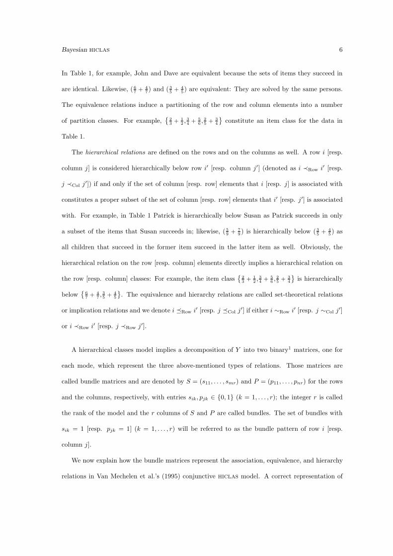
In Table 1, for example, John and Dave are equivalent because the sets of items they succeed in

are identical. Likewise, ( 6

7+ 4

7) and ( 3

5+ 4

5) are equivalent: They are solved by the same persons.

The equivalence relations induce a partitioning of the row and column elements into a number

of partition classes. For example,{

2

3+ 1

2, 3

4+ 5

6, 2

5+ 3

4

}constitute an item class for the data in

Table 1.

The hierarchical relations are defined on the rows and on the columns as well. A row i [resp.

column j] is considered hierarchically below row i′ [resp. column j′] (denoted as i ≺Row i′ [resp.

j ≺Col j′]) if and only if the set of column [resp. row] elements that i [resp. j] is associated with

constitutes a proper subset of the set of column [resp. row] elements that i′ [resp. j′] is associated

with. For example, in Table 1 Patrick is hierarchically below Susan as Patrick succeeds in only

a subset of the items that Susan succeeds in; likewise, ( 5

9+ 7

9) is hierarchically below ( 3

5+ 4

5) as

all children that succeed in the former item succeed in the latter item as well. Obviously, the

hierarchical relation on the row [resp. column] elements directly implies a hierarchical relation on

the row [resp. column] classes: For example, the item class{

2

3+ 1

2, 3

4+ 5

6, 2

5+ 3

4

}is hierarchically

below{

6

7+ 4

7, 3

5+ 4

5

}. The equivalence and hierarchy relations are called set-theoretical relations

or implication relations and we denote i �Row i′ [resp. j �Col j′] if either i ∼Row i′ [resp. j ∼Col j′]

or i ≺Row i′ [resp. j ≺Row j′].

A hierarchical classes model implies a decomposition of Y into two binary1 matrices, one for

each mode, which represent the three above-mentioned types of relations. Those matrices are

called bundle matrices and are denoted by S = (s11, . . . , smr) and P = (p11, . . . , pnr) for the rows

and the columns, respectively, with entries sik, pjk ∈ {0, 1} (k = 1, . . . , r); the integer r is called

the rank of the model and the r columns of S and P are called bundles. The set of bundles with

sik = 1 [resp. pjk = 1] (k = 1, . . . , r) will be referred to as the bundle pattern of row i [resp.

column j].

We now explain how the bundle matrices represent the association, equivalence, and hierarchy

relations in Van Mechelen et al.’s (1995) conjunctive hiclas model. A correct representation of

Bayesian hiclas 7

the association relation implies for any i and j:

yij =

1 if ∀k(1 ≤ k ≤ r) : sik ≥ pjk

0 otherwise.

(1)

Equation (1) means that a row is associated with a column if and only if the column’s bundle

pattern is a (proper or improper) subset of the row’s bundle pattern. Table 2 shows the bundle

matrices S and P of a conjunctive model in rank 3 for the hypothetical matrix in Table 1. We find

that, for example, John’s bundle pattern ({II, III}) includes all the bundles in the pattern of item

( 6

7+ 4

7) ({II}) while Table 1 shows that John succeeds in the item; similarly, John does not solve

( 1

4+ 2

3) as his bundle pattern lacks Bundle I, which is included in the item’s bundle pattern.

Optionally one may look for a substantive interpretation of the bundles and the association rule

in the example: The three bundles may be regarded as underlying abilities that children either

have (sik = 1) or do not have (sik = 0), and that are either required (pjk = 1) or not required

(pjk = 0) for solving the item. In particular, Bundle I can be interpreted as the ability of finding the

lowest common multiple of two integers (needed to reduce two fractions to a common denominator),

Bundle II can be interpreted as the ability of dealing with fractions where the denominator exceeds

the nominator, and Bundle III as the ability of finding the greatest common divisor of two integers

(needed to reduce a fraction as far as possible). Then, Eq. (1) can be read as: A child succeeds in

an item if and only if (s)he has all the abilities required by the item.

The conjunctive hierarchical classes model further adds the following restriction on S and P to

represent the set-theoretical relations :

∀i, i′ : i �Row i′ iff ∀k(1 ≤ k ≤ r) : sik ≤ si′k (2a)

∀j, j′ : j �Col j′ iff ∀k(1 ≤ k ≤ r) : pjk ≥ pj′k. (2b)

A pair of bundle matrices (S, P ) for which (2a) and (2b) hold are called set-theoretically consistent.

Eq. (2a) [resp. Eq. (2b)] implies that equivalent rows [resp. columns] have identical bundle patterns.

In the example of Table 2, John and Dave, who are equivalent in Table 1, have an identical set

of abilities. Eq. (2a) further implies that, if row i is hierarchically below row i′, then the bundle

pattern of i is a proper subset of the bundle pattern of i′. In Table 2, for example, Mary’s abilities

Bayesian hiclas 8

include as a proper subset those of John and Dave, who are hierarchically below Mary. On the other

hand, Eq. (2b) implies that if column j is hierarchally below column j′ then the bundle pattern

of j is a proper superset of the bundle pattern of j′. The items in class{

23 + 1

2 , 34 + 5

6 , 25 + 3

4

}, for

example, which is hierarchically below the item class{

67 + 4

7 , 35 + 4

5

}, require a proper superset of

the abilities required by the latter items ({I, II} ⊃ {II}). Within an ability context the inverse

representation of the item hierarchy naturally follows from the fact that the more abilities are

required by an item, the less children dominate it.

2.2 Graphical representation

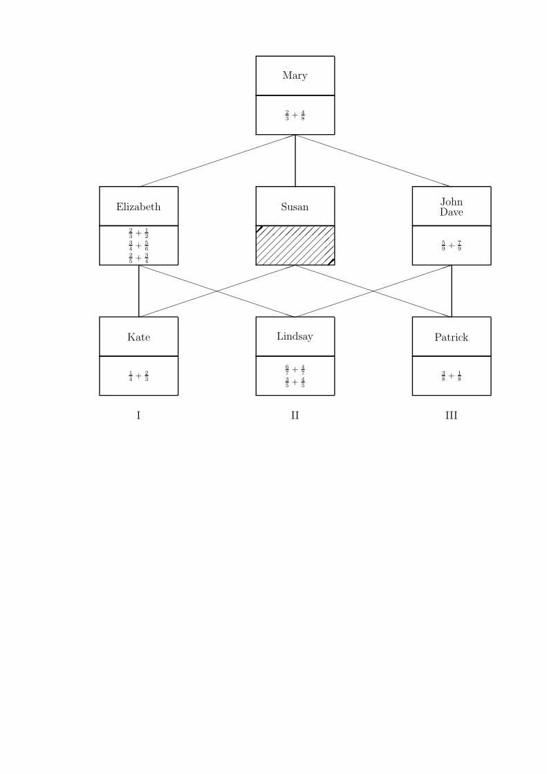
Van Mechelen et al. (1995) proposed a graphical representation that gives a full account of the

relations represented by the conjunctive hierarchical classes model. A graphical representation of

the model in Table 2 is found in Figure 1. In the graphical representation, the child and item classes

appear as paired boxes, the upper box of each pair being a child class and the lower box an item

class. The lines connecting the classes represent the hierarchical relations, with the item hierarchy

to be read upside down. The association relation can be read from the graph as a dominance

relation: A child succeeds in all items below him/her and an item is solved by all children above

it.

2.3 Data analysis

Van Mechelen et al. (1995) (relying on a proposition by De Boeck and Rosenberg, 1988) showed

that a perfectly fitting hierarchical classes model can be found for any matrix Y . However, in

most realistic applications, models of high rank are needed for an exact decomposition of Y , such

that the resulting model is often difficult to interpret. Therefore, in practice one usually searches

for an approximate reconstructed data matrix Y that can be represented by a low rank hiclas

model. In particular, in a typical hiclas analysis (De Boeck and Rosenberg, 1988; Leenen and

Van Mechelen, 2001), a matrix Y for which a hierarchical classes model in some prespecified rank

Bayesian hiclas 9

r holds is looked for such that the loss function

D(Y , Y ) =∑

i,j

(yij − yij)2 (3)

has minimal value. Note that, since Y and Y only contain 0/1 values, the least squares loss function

in Eq. (3) comes down to a least absolute deviations loss function (Chaturvedi and Carroll, 1997),

and equals the number of discrepancies between Y and Y .

2.4 Model checking and drawing inferences

Although yielding quite satisfactory results in general, the widespread use of finding a best-fitting

hiclas model Y for given data Y is conceptually unclear. For, as in all deterministic models, in

an approximate hiclas model, the relation to the data is not specified (i.e., it is not specified how

and why predictions by the model may differ from the observed data), and hence, the slightest

deviation between model and data strictly speaking implies a rejection of the model. Furthermore,

because the model either fully holds or is rejected as a whole, it does not make sense to develop

checks for specific model assumptions.

Furthermore, in most practical applications, the basis for pre-specifying the rank r of an ap-

proximating hiclas model for Y is often unclear. As a way out, a number of heuristics have been

developed to infer a rank from the data, which in most cases is based on comparing the goodness-

of-fit values for models of successive ranks. Examples of such heuristics include variants of the

scree test and Leenen and Van Mechelen’s (2001) pseudo-binomial test. Although these heuristics

may yield satisfactory results, in some cases the selection of a particular rank seems arbitrary and

susceptible to chance.

3 Stochastic extension within a Bayesian framework

3.1 Model

The standard hiclas approach with its search for an approximate solution that has an optimal fit

to a given data set reveals the assumption of an underlying stochastic process that may cause the

Bayesian hiclas 10

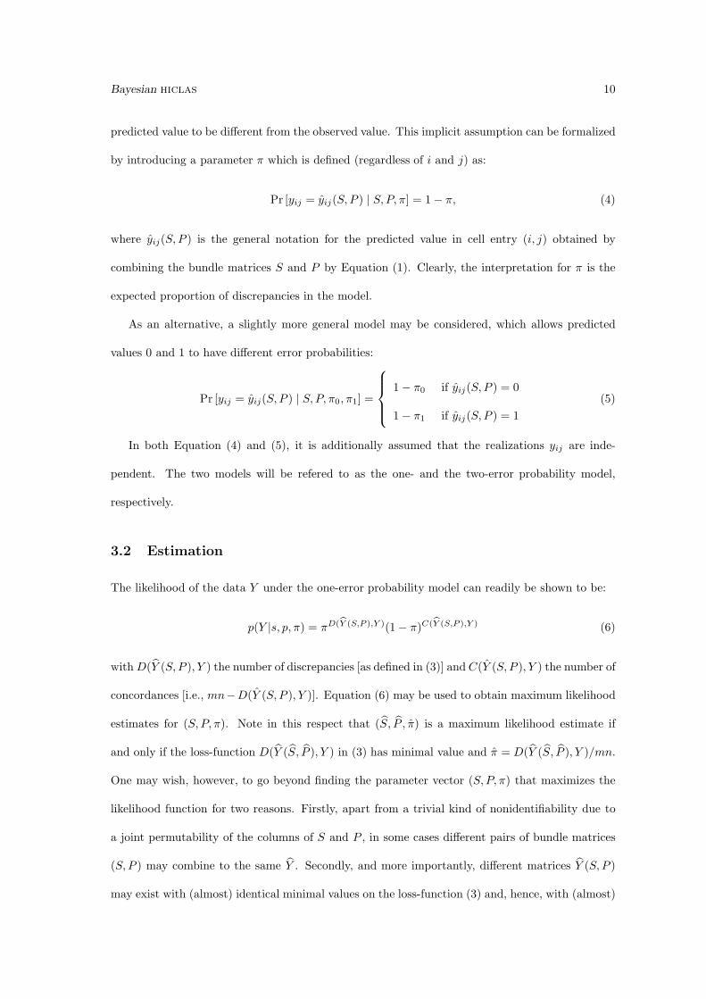
predicted value to be different from the observed value. This implicit assumption can be formalized

by introducing a parameter π which is defined (regardless of i and j) as:

Pr [yij = yij(S, P ) | S, P, π] = 1− π, (4)

where yij(S, P ) is the general notation for the predicted value in cell entry (i, j) obtained by

combining the bundle matrices S and P by Equation (1). Clearly, the interpretation for π is the

expected proportion of discrepancies in the model.

As an alternative, a slightly more general model may be considered, which allows predicted

values 0 and 1 to have different error probabilities:

Pr [yij = yij(S, P ) | S, P, π0, π1] =

1− π0 if yij(S, P ) = 0

1− π1 if yij(S, P ) = 1

(5)

In both Equation (4) and (5), it is additionally assumed that the realizations yij are inde-

pendent. The two models will be refered to as the one- and the two-error probability model,

respectively.

3.2 Estimation

The likelihood of the data Y under the one-error probability model can readily be shown to be:

p(Y |s, p, π) = πD(Y (S,P ),Y )(1− π)C(Y (S,P ),Y ) (6)

with D(Y (S, P ), Y ) the number of discrepancies [as defined in (3)] and C(Y (S, P ), Y ) the number of

concordances [i.e., mn−D(Y (S, P ), Y )]. Equation (6) may be used to obtain maximum likelihood

estimates for (S, P, π). Note in this respect that (S, P , π) is a maximum likelihood estimate if

and only if the loss-function D(Y (S, P ), Y ) in (3) has minimal value and π = D(Y (S, P ), Y )/mn.

One may wish, however, to go beyond finding the parameter vector (S, P, π) that maximizes the

likelihood function for two reasons. Firstly, apart from a trivial kind of nonidentifiability due to

a joint permutability of the columns of S and P , in some cases different pairs of bundle matrices

(S, P ) may combine to the same Y . Secondly, and more importantly, different matrices Y (S, P )

may exist with (almost) identical minimal values on the loss-function (3) and, hence, with (almost)

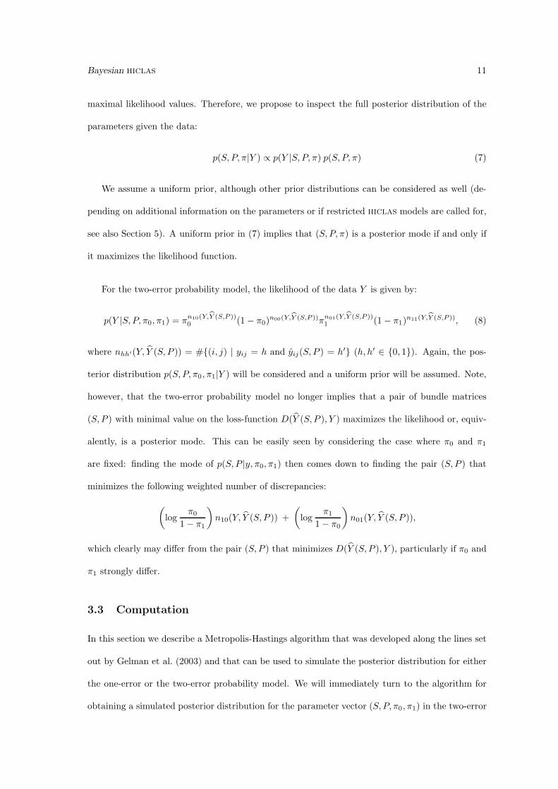
Bayesian hiclas 11

maximal likelihood values. Therefore, we propose to inspect the full posterior distribution of the

parameters given the data:

p(S, P, π|Y ) ∝ p(Y |S, P, π) p(S, P, π) (7)

We assume a uniform prior, although other prior distributions can be considered as well (de-

pending on additional information on the parameters or if restricted hiclas models are called for,

see also Section 5). A uniform prior in (7) implies that (S, P, π) is a posterior mode if and only if

it maximizes the likelihood function.

For the two-error probability model, the likelihood of the data Y is given by:

p(Y |S, P, π0, π1) = πn10(Y,Y (S,P ))0 (1− π0)

n00(Y,Y (S,P ))πn01(Y,Y (S,P ))1 (1− π1)

n11(Y,Y (S,P )), (8)

where nhh′(Y, Y (S, P )) = #{(i, j) | yij = h and yij(S, P ) = h′} (h, h′ ∈ {0, 1}). Again, the pos-

terior distribution p(S, P, π0, π1|Y ) will be considered and a uniform prior will be assumed. Note,

however, that the two-error probability model no longer implies that a pair of bundle matrices

(S, P ) with minimal value on the loss-function D(Y (S, P ), Y ) maximizes the likelihood or, equiv-

alently, is a posterior mode. This can be easily seen by considering the case where π0 and π1

are fixed: finding the mode of p(S, P |y, π0, π1) then comes down to finding the pair (S, P ) that

minimizes the following weighted number of discrepancies:

(log

π0

1− π1

)n10(Y, Y (S, P )) +

(log

π1

1− π0

)n01(Y, Y (S, P )),

which clearly may differ from the pair (S, P ) that minimizes D(Y (S, P ), Y ), particularly if π0 and

π1 strongly differ.

3.3 Computation

In this section we describe a Metropolis-Hastings algorithm that was developed along the lines set

out by Gelman et al. (2003) and that can be used to simulate the posterior distribution for either

the one-error or the two-error probability model. We will immediately turn to the algorithm for

obtaining a simulated posterior distribution for the parameter vector (S, P, π0, π1) in the two-error

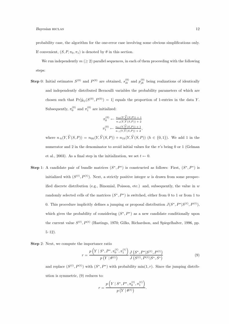
Bayesian hiclas 12

probability case, the algorithm for the one-error case involving some obvious simplifications only.

If convenient, (S, P, π0, π1) is denoted by θ in this section.

We run independently m (≥ 2) parallel sequences, in each of them proceeding with the following

steps:

Step 0: Initial estimates S(0) and P (0) are obtained, s(0)ik and p

(0)jk being realizations of identically

and independently distributed Bernoulli variables the probability parameters of which are

chosen such that Pr[yij(S(0), P (0)) = 1] equals the proportion of 1-entries in the data Y .

Subsequently, π(0)0 and π

(0)1 are initialized:

π(0)0 ← n10(Y,Y (S,P )) + 1

n·0(Y,Y (S,P )) + 2

π(0)1 ← n01(Y,Y (S,P )) + 1

n·1(Y,Y (S,P )) + 2,

where n·h(Y, Y (S, P )) = n0h(Y, Y (S, P )) + n1h(Y, Y (S, P )) (h ∈ {0, 1}). We add 1 in the

numerator and 2 in the denominator to avoid initial values for the π’s being 0 or 1 (Gelman

et al., 2003). As a final step in the initialization, we set t← 0.

Step 1: A candidate pair of bundle matrices (S∗, P ∗) is constructed as follows: First, (S∗, P ∗) is

initialized with (S(t), P (t)). Next, a strictly positive integer w is drawn from some prespec-

ified discrete distribution (e.g., Binomial, Poisson, etc.) and, subsequently, the value in w

randomly selected cells of the matrices (S∗, P ∗) is switched, either from 0 to 1 or from 1 to

0. This procedure implicitly defines a jumping or proposal distribution J(S∗, P ∗|S(t), P (t)),

which gives the probability of considering (S∗, P ∗) as a new candidate conditionally upon

the current value S(t), P (t) (Hastings, 1970; Gilks, Richardson, and Spiegelhalter, 1996, pp.

5–12).

Step 2: Next, we compute the importance ratio

r =p(Y | S∗, P ∗, π

(t)0 , π

(t)1

)

p(Y | θ(t)

) J(S∗, P ∗|S(t), P (t)

)

J(S(t), P (t)|S∗, S∗

) (9)

and replace (S(t), P (t)) with (S∗, P ∗) with probability min(1, r). Since the jumping distrib-

ution is symmetric, (9) reduces to:

r =p(Y | S∗, P ∗, π

(t)0 , π

(t)1

)

p(Y | θ(t)

) .

Bayesian hiclas 13

Step 3: π(t)0 and π

(t)1 are updated by drawing from a Beta

[n10(Y, Y (S(t), P (t))) + 1, n00(Y, Y (S(t), P (t))) + 1

]

and a Beta[n01(Y, Y (S(t), P (t))) + 1, n11(Y, Y (S(t), P (t))) + 1

]distribution, respectively.

Step 4: If the pair of bundle matrices (S(t), P (t)) is set-theoretically consistent, then we set (a)

θ(t+1) ← θ(t) and, subsequently, (b) t← t + 1;

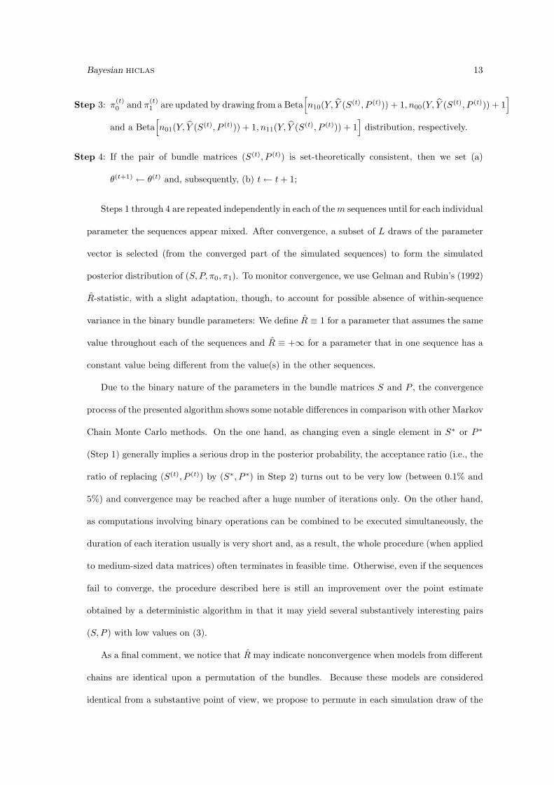
Steps 1 through 4 are repeated independently in each of the m sequences until for each individual

parameter the sequences appear mixed. After convergence, a subset of L draws of the parameter

vector is selected (from the converged part of the simulated sequences) to form the simulated

posterior distribution of (S, P, π0, π1). To monitor convergence, we use Gelman and Rubin’s (1992)

R-statistic, with a slight adaptation, though, to account for possible absence of within-sequence

variance in the binary bundle parameters: We define R ≡ 1 for a parameter that assumes the same

value throughout each of the sequences and R ≡ +∞ for a parameter that in one sequence has a

constant value being different from the value(s) in the other sequences.

Due to the binary nature of the parameters in the bundle matrices S and P , the convergence

process of the presented algorithm shows some notable differences in comparison with other Markov

Chain Monte Carlo methods. On the one hand, as changing even a single element in S∗ or P ∗

(Step 1) generally implies a serious drop in the posterior probability, the acceptance ratio (i.e., the

ratio of replacing (S(t), P (t)) by (S∗, P ∗) in Step 2) turns out to be very low (between 0.1% and

5%) and convergence may be reached after a huge number of iterations only. On the other hand,

as computations involving binary operations can be combined to be executed simultaneously, the

duration of each iteration usually is very short and, as a result, the whole procedure (when applied

to medium-sized data matrices) often terminates in feasible time. Otherwise, even if the sequences

fail to converge, the procedure described here is still an improvement over the point estimate

obtained by a deterministic algorithm in that it may yield several substantively interesting pairs

(S, P ) with low values on (3).

As a final comment, we notice that R may indicate nonconvergence when models from different

chains are identical upon a permutation of the bundles. Because these models are considered

identical from a substantive point of view, we propose to permute in each simulation draw of the

Bayesian hiclas 14

Metropolis-Hastings algorithm to the solution that minimizes the difference with some prespecified

reference model (S, P ) (for example, the model obtained from the original deterministic algorithm).

That is, after each iteration t a permutation of the bundles in (S(t), P (t)) is found such that

∑

i,j

(yij(S

(t), P (t))− yij(S, P ))2

has minimal value. Whereas the choice of the reference model may affect the convergence rate,

posterior inferences with respect to the association, equivalence, and hierarchy relations based on

the converged simulated posterior distribution remain unaffected by the choice of (S, P ).

3.4 Representation of the posterior distribution

In contrast with the deterministic model, in which for a particular pair of elements (or classes)

the association, equivalence, and hierarchy relations either hold or do not hold, the new stochastic

extension implies a (marginal) posterior probability for any individual relation. In order to repre-

sent this posterior uncertainty, one can make use both of tabular form and of an adapted version

of Van Mechelen et al.’s (1995) original graphical representation.

To chart out the uncertainty in the association relation, for each row-column pair the proportion

of the L simulation draws in which the row is associated with the column can be calculated and

the results can be represented in an m by n table. Similarly, marginal posterior probabilities for

the equivalence and hierarchy relations can be calculated and given a tabular representation, both

for the row elements and the column elements.

In the adapted graphical representation, each class is represented with a box (as before), which

now contains all elements for which the marginal posterior probability of belonging to the class

exceeds some prespecified cut-off α. Furthermore, the uncertainty in the hierarchical relation

among classes can be represented in the graph by varying the line thickness or by labeling the

edges. To quantify the degree of certainty of the hierarchical relation C1 ≺ C2 between any pair

of row classes (C1, C2), we propose the following measure:

p(C1 ≺Row C2) =

m∑i=1

m∑i′=1

p(i ∈ C1) p(i′ ∈ C2) p(i ≺Row i′)

m∑i=1

m∑i′=1

p(i ∈ C1) p(i′ ∈ C2),

Bayesian hiclas 15

where p(i ∈ Ck) is the posterior probability of row i belonging to row class Ck and p(i ≺Row i′) is

the posterior probability of row i being hierarchically below row i′. The strength of the hierarchical

relations among the column classes can be calculated through a similar formula.

3.5 Model checking and drawing inferences

Within a Bayesian framework a broad range of tools for model checking is available. In this

section, we will discuss the use of posterior predictive checks (ppc’s) for model selection and model

checking (Rubin, 1984; Gelman, Meng, and Stern, 1996). The rationale of ppc’s is the comparison,

via some test quantity, of the observed data with data that could have been observed if the actual

experiment were replicated under the model with the same parameters that generated the observed

data (Gelman, Carlin, Stern, and Rubin, 1995). The test quantity may be a statistic T (Y ),

summarizing some aspect of the data, or, more generally, a discrepancy measure T (Y, S, P, π0, π1)

quantifying the model’s deflection from the data in some respect (Meng, 1994).

The ppc procedure consists of three substeps. First, for each of the draws θl ≡ (Sl, P l, πl0, π

l1)

(l = 1, . . . , L) from the simulated posterior distribution, a replicated data set Y rep l is simulated,

each cell entry yrep lij being an independent realization of a Bernoulli variable with probability

parameter |h − πlh|, where h = yij(s

l, pl). Second, for each simulated draw, the value of the

test quantity is calculated for both the observed data Y obs (i.e., T (Y obs, θl)) and the associated

replicated data Y rep l (i.e., T (Y rep l, θl)). As a final step, the values for the observed and the

replicated data are compared and the proportion of simulation draws for which T (Y rep l, θl) >

T (Y obs, θl) is considered as an estimate of the posterior predictive p-value.

Different aspects of the model can be checked using ppc’s with appropriate choices of the

test quantity. In the remainder of this section, we will elaborate some ppc’s for checking (1) the

deterministic core of the model and (2) the error structure as implied by the stochastic part of the

model. These checks will be further illustrated in the application of Section 4.

Bayesian hiclas 16

3.5.1 Checking the deterministic core of the model

Rank The ppc procedure can be used as a tool for rank selection by defining a test quantity

that is sensitive to the underestimation of the rank r. That is, assuming that some true hiclas

model underlies the observed data, the test quantity should yield higher values if the rank of the

fitted model is lower than the rank of the true model. To this end, we define a test statistic T (Y )

that is the improvement on the loss-function (3) gained by adding an extra bundle to the model

in rank r. More precisely:

T (Y ) = D(Y r+1, Y )−D(Y r, Y ), (10)

where Y k (k = r, r+1) is the deterministic model matrix obtained by applying the original hiclas

algorithm (De Boeck and Rosenberg, 1988; Leenen and Van Mechelen, 2001) in rank k to the

data set Y . If the true rank underlying the observed data is larger than r, then the fit of a rank

r + 1 model will substantially increase compared to the fit of the rank r model, and the value of

T (Y obs) will be expected to be higher than the values T (Y rep l) for the replicated data sets. For,

the underlying true rank in the latter data sets is of rank r and the extra bundle in the r+1 model

only fits noise.

Set-theoretical relations As a second example, we will test the conformity of the set-theoretical

relations represented in the model with those in the data. Possibly the model is either too conser-

vative or too liberal in the representation of the equivalence and hierarchy relations. To this end,

we will compare, for each pair of rows i and i′ [resp. columns j and j′], the presence/abscence of

an implication relation i �Row i′ [resp. j �Col j′] in the model with their implicational strength in

the data. As a measure for the latter, we will use conditional probabilities

p(yi′·|yi·) ≡

∑j

yijyi′j

∑j

yij

and p(y·j′ |y·j) ≡

∑i

yijyij′

∑i

yij

(p(yi′·|yi·)

[resp. p(y

·j′ |y·j)]

being considered undefined whenever∑j

yij = 0[resp.

∑i

yij = 0])

.

Then, the test quantity used in the ppc for the row set-theoretical relations is defined as:

T (Y, S) =

m∑

i=1

m∑

i′=1

∣∣∣p(yi′·|yi·)− IS(i �Row i′)∣∣∣, (11a)

Bayesian hiclas 17

where the first summation is across rows i with∑j

yij 6= 0 and IS(i �Row i′) takes a value of 1 if

the bundle matrix S implies i �Row i′, and 0 otherwise. A similar test quantity for the column

set-theoretical relations may be defined:

T (Y, P ) =

n∑

j=1

n∑

j′=1

∣∣∣p(y·j′ |y·j)− IP (j �Col j′)

∣∣∣, (11b)

where the first summation is across columns j with∑i

yij 6= 0.

3.5.2 Checking the error model

One-probability versus two-probability model For a check of the validity of the one-error

model (4) against the alternative model (5) with two error parameters, it is straightforward to use

a test quantity that compares the proportion of discrepancies in cells where yij(S, P ) = 0 with the

proportion of discrepancies in cells where yij(S, P ) = 1, for example by calculating the difference:

T (Y, S, P ) =n10(Y, Y (S, P ))

n·0(Y, Y (S, P ))−

n01(Y, Y (S, P ))

n·1(Y, Y (S, P )). (12)

The test quantity in Eq. (12) is the difference between the maximum likelihood estimates of π0

and π1, respectively, for fixed S and P under the two-error model. In data sets replicated under

the one-error model, the expected value of T (Y rep l, Sl, P l) equals 0. Values of T (Y obs, Sl, P l)

that are found to be more extreme than T (Y rep l, Sl, P l) may indicate a violation of the one error

parameter assumption.

Homogeneity of the error process The assumption π0 = π1 = π is part of a more general

assumption of a homogeneous error parameter structure across all data points implied by model

(4). Incidentally, the latter assumption is conceptually similar to the homoscedasticity assumption

of equal error variances across observations in regression models or in analysis of variance. Within

a Bayesian framework, deviations from this general assumption can be checked easily. The model,

for example, implies the assumption of equal error probability parameters across rows, which may

be too restrictive. This assumption can be checked with the variance of the number of discrepancies

across rows,

T (Y, S, P ) =m∑

i=1

(Di·(Y (S, P ), Y )

)2

−1

m

(m∑

i=1

Di·(Y (S, P ), Y )

)2

(13a)

Bayesian hiclas 18

with Di·

(Y (S, P ), Y

)=

n∑j=1

[yij(S, P )− yij

]2, which will tend to be higher if the error probability

parameter differs across rows. Similarly, the assumption of equal error probabilities across columns

can be checked using the variance of the number of discrepancies across columns as a test quantity:

T (Y, S, P ) =n∑

j=1

(D·j(Y (S, P ), Y )

)2

−1

n

n∑

j=1

D·j(Y (S, P ), Y )

2

(13b)

with D·j

(Y (S, P ), Y

)=

m∑i=1

[yij(S, P )− yij

]2.

4 Application

In this section we present a reanalysis of person by choice object select/nonselect data (i.e., so-

called pick any/n data, Coombs, 1964, p. 295), that were previously analyzed by Van Mechelen and

Van Damme (1994). These data originate from each of 26 second-year psychology students being

presented with 25 index cards with room descriptions from the Housing Service of the University

of Leuven and being asked to select those rooms (s)he would decide to visit when looking for a

student room. (Most students in Leuven rent a room during the academic year and many of them

pass by the Housing Service to get an overview and descriptions of the available rooms.) This

resulted in a 26 × 25 binary matrix Y with yij = 1 if student i selected room j, and yij = 0

otherwise.

In the original study, Van Mechelen and Van Damme analyzed these data using a deterministic

conjunctive hiclas model with an interpretation of the bundles in terms of latent choice criteria.

The key idea behind their interpretation was that the rooms selected by a person are those that

meet all his (her) criteria. This idea is formalized by a variant of the conjunctive hiclas model

with the bundle matrix S denoting the persons’ choice criteria and the bundle matrix P the

corresponding properties of the rooms and with the following association rule2:

yij =

1 if ∀k(1 ≤ k ≤ r) : pjk ≥ sik

0 otherwise.

Here we apply a Bayesian hiclas model to the same data. First, we fitted a rank 1 model

with one error probability parameter. In the Metropolis-Hastings algorithm, 5 sequences were

Bayesian hiclas 19

used and in the jumping procedure the number of entries to be changed was drawn from a Poisson

distribution with parameter λ = 4. Convergence was reached (for all parameters, R < 1.05) after

about 1.5 million of iterations (i.e., after less than ten minutes on a Pentium IV 3.06 gHz). To

save computer resources, each thousandth draw in the second half of the 5 sequences (these were

also the draws on which the convergence statistic was calculated), was saved, so that we are left

with about 3,500 simulated posterior draws.

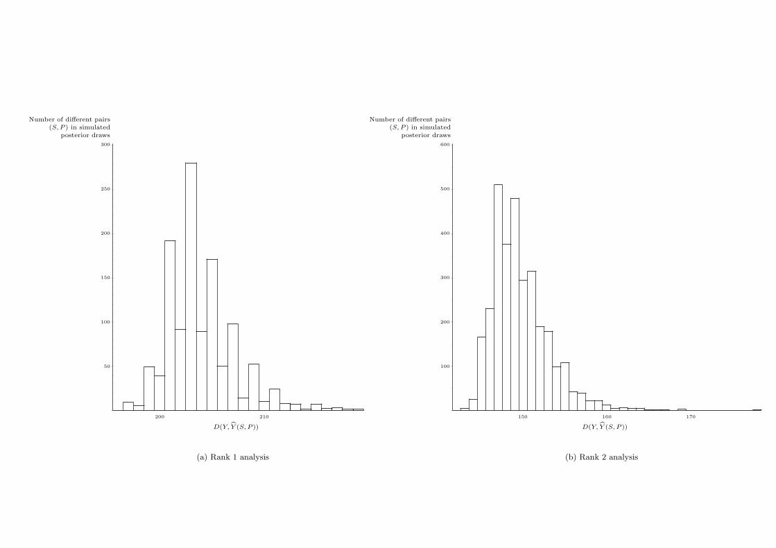
Figure 2(a) shows how many different pairs of bundle matrices (S, P ) were found in the simu-

lated marginal posterior distribution of the rank 1 model (with π being integrated out) at each value

of D(Y (S, P ), Y ). Clearly, for the data set under study, the deterministic approach would suffer

from multimodality: Nine different models were found with a minimal number of discrepancies.

Moreover, many more models come close to this lower bound. Yet, applying the original deter-

ministic algorithm would return a single model, keeping the user unaware of possible alternative

models with an (almost) equally low number of discrepancies.

The rank 1 model is too simple, though, to give a good account of the data: Using the ppc

procedure based on the test statistic (10) for detecting underestimation of the rank, the model in

rank 1 is rejected (T = 54, ppc-p = .02). Therefore, we applied the Metropolis-Hastings algorithm

to obtain a simulated posterior distribution for the conjunctive rank 2 model as well. With the

same settings as in the analysis for the rank 1 model (except that for the Poisson distribution, a

parameter λ = 6 was used to account for the larger number of parameters in the bundle matrices),

we found convergence after about 17.5 million iterations (i.e., after about one hour on a Pentium

IV 3.06 gHz). Each ten thousandth draw in the second half of the 5 sequences was saved to obtain

a set of about 4,400 posterior draws. A ppc procedure with statistic (10) to test a rank 2 against

a rank 3 model now yielded T = 27 (ppc-p = .12); therefore, the rank 2 model was retained for

further discussion. From Figure 2(b), we can read how many different pairs of bundle matrices

of rank 2 were found at each value D(Y (S, P ), Y ). In particular, 4 different pairs (S, P ) with a

minimal number of 143 discrepancies were found, and 25 other models had only one discrepancy

more. Again, thanks to the new approach, multi-modality was traced.

Bayesian hiclas 20

For the obtained model in rank 2, we further illustrate the use of the three other statistics

for checking some model assumptions that we presented in Section 3.5. First, with regard to the

comformity of the set-theoretical relations in the model with those in the data, the ppc p-value

with test quantity (11a) is found to be equal to .41 and with test quantity (11b) .40. In other

words, no evidence is found for an inconsistency between the implication relations as represented

in the model and the corresponding relations in the data. Second, the assumption of equal error

probabilities for predicted 0’s and 1’s as implied by the one-error probability model is checked with

test quantity (12). The mean value on the latter test quantity equals .00 for the replicated data,

as expected on theoretical grounds, and −.02 for the observed data. Furthermore, T (Y obs, Sl, P l)

exceeds T (Y rep l, Sl, P l) in 31% of the cases, from which we may conclude that the one-error

probability model has not to be replaced with the more general two-error probability model. Third,

the homogeneity assumption of the error across students is tested by means of the variance in the

number of discrepancies across students (Eq. 13a). A higher variance for the observed data could

have been likely if, for example, students differed in the level of engagement when completing

the task. However, the ppc p-value of .73 provides no evidence for individually different error

parameters. In the same way, a test using the variance in the number of discrepancies across

rooms (Eq. 13b) is performed. Such a test could reveal, for example, differences in quality of the

room discriptions. Yet, the ppc p-value of .43 does not provide any indication for extending the

model with different error parameters across rooms.

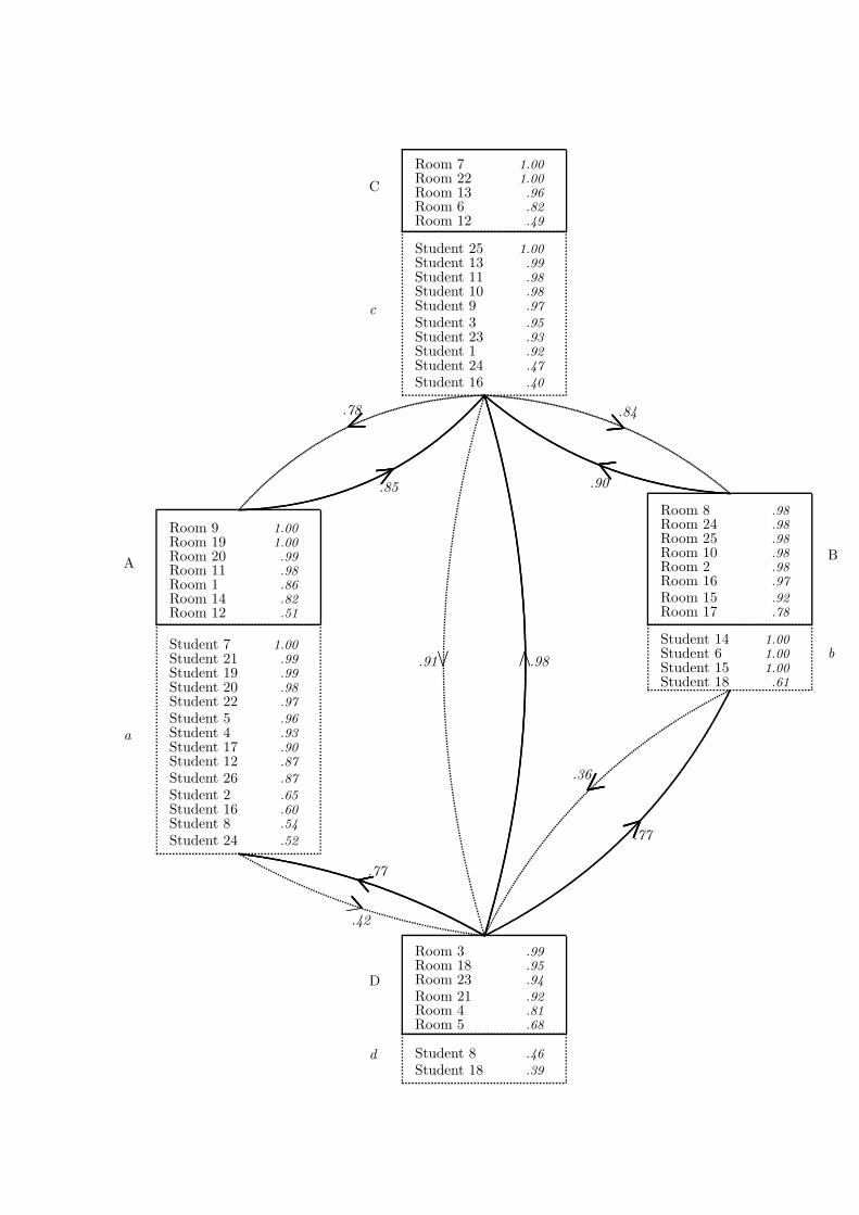
Figure 3 displays a graphical representation of the simulated posterior distribution of the rank

2 model, from which we can read the three types of relations: (i) association, (ii) classification, and

(iii) hierarchy. (i) The association relation can be read deterministically as in the original model:

Rooms are selected by any student who is below it. For example, if we ignore the uncertainty in

the association relation for a moment, it holds that the rooms in cluster C are selected by all the

students, whereas those from cluster B are selected by the students in clusters b and d only. The

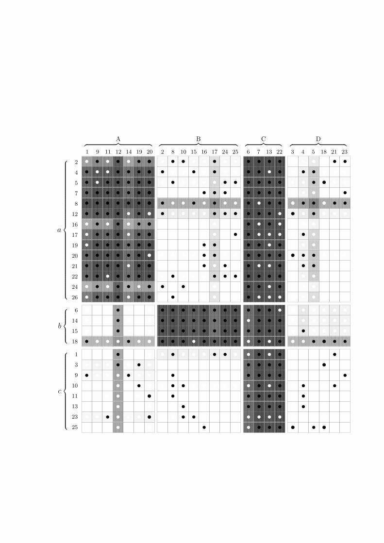
uncertainty in the association relation is not directly represented in the graph, though. Figure

4, however, shows the marginal posterior probabilities for each room-student association using

Bayesian hiclas 21

gray values, with darker values corresponding with higher selection probabilities. The dot in the

center of each cell, either black or white, represent the observed data value and allows to check the

degree of discrepancy between the model and the data with respect to the association relation. (ii)

Concerning the classifications, row and column classes appear in the paired boxes of Figure 3, with

in the solid-framed box of each pair a row (room) cluster and in the dotted-framed box a column

(student) cluster. The uncertainty with respect to the clustering is represented by the marginal

posterior probability for each element to belong to the particular cluster. Only elements for which

the posterior probability exceeds α = .33 are displayed in the box. So, we can read, for instance,

that Room 7 is found to be in cluster C in all the simulation draws whereas Room 12 is found

about evenly in the clusters A and C. (iii) The room and student hierarchies are represented by

solid and dotted arrows, respectively, connecting any two clusters C1 and C2 for which the strength

of the hierarchical relation C1 ≺ C2 (as explained in Section 3.4) exceeds α = .33. Student cluster

a, for instance, is found to be hierarchically below cluster d, though weakly (.42), whereas room

cluster B is strongly (.90) hierarchically below room cluster C.

Figures 3 and 4 illustrate that, although many different pairs of bundle matrices (S, P ) were

found to have a minimal or near-minimal value on the loss-function, the hierarchical classes struc-

ture does have a stable part: For example, in almost all simulation draws, Rooms 7, 22, and 13,

were found in the same class (at the top of the hierarchy). With regard to the substantive inter-

pretation of the model, we follow Van Mechelen and Van Damme (1994) who conceived the two

bundles as latent choice criteria. From the description of the rooms on the index cards, the first

bundle, on which room clusters A and C load, appears to be related to “Elementary comfort +

Good quality”, whereas the rooms of clusters B and C, which load on the second bundle, appear

to have as a distinctive characteristic “Elementary comfort + Low price” . The rooms in cluster

D, at the bottom of the hierarchy, differ from the other rooms in that these rooms lack elementary

comfort (such as water and kitchen facilities). The posterior probability of belonging to cluster

d being low for all students, we can conclude that all students consider elementary comfort as a

necessary prerequisite for a room to be selected. The students in cluster a additionally require

Bayesian hiclas 22

the rooms to be of a good quality (mainly large and quiet) and the students in cluster b have a

low price as additional requisite; students in cluster c, at last, select rooms that have both good

quality and low price.

5 General discussion

This paper presented a new stochastic extension of the original deterministic hierarchical classes

model (De Boeck and Rosenberg, 1988; Van Mechelen et al., 1995) in response to a number

of conceptual and practical problems. Conceptually, the benefit of the new extension is that

the relation between the predicted values and the observed values is made explicit thanks to

the inclusion of one or two error-probability parameters. This enabled us to consider the model

within a Bayesian framework and to make use of a variety of tools for model estimation and

model checking. As shown in the example, this approach leads to a more differentiated view

on the solution space by revealing several models that fit the data (almost) equally well. This

differentiation may result in a fine-tuned interpretation in which core and peripheral aspects of the

resulting structure are distinguished. Unlike the probabilistic variant developed by Maris et al.

(1996), this differentiation is obtained without leaving or “fuzzifying” the set-theoretical or logical

framework of the original hiclas model. As such, the new model fully retains the deterministic core

of the model, including the representation of the set-theoretical relations, while by superimposing

the stochastic framework, the uncertainty in those set-theoretical relations is fully accounted for.

More specifically, it is possible to evaluate the strength of the implication relations (which directly

follows from the hierarchies represented in the model) by making use of the simulated posterior

distribution of the parameters. In this respect, both simple implications (of the type if A then B)

and more complex implications (e.g., if A or B then C) can be considered.

The new model extension as presented here may be extended further in various directions.

For example, the model includes only one or two probability parameters, but additional error

parameters may be introduced based on some hypotheses about the error process at hand. Such

hypotheses may be either a priori or may result from model checks that indicate a misfit with respect

Bayesian hiclas 23

to a particular assumption (like, for example, the assumption of equal error probabilities across rows

and columns). A second direction in which the model can be further extended relates to the choice

of the prior distribution. We choosed a uniform distribution for the set of parameters, implying

that any hierarchical classes model is considered equally likely a priori and that the posterior

distribution is proportional to the likelihood. Alternative prior distributions may be considered,

motivated either by former results or by restrictions one may wish to add to the hiclas model (for

example, the restriction that the hierarchies constitute total orders rather than partial orders, or

that the hierarchical relationship among some elements is fixed, etc.). Such restrictions can easily

be incorporated by assigning a low or zero probability in the prior distribution to models that do

not satisfy them. The Metropolis-Hastings algorithm for simulating the posterior distribution can

be adapted accordingly either by changing the jumping rule or by dropping models that do not

satisfy the restrictions.

Finally, one may point at an interesting relation between the model extension as proposed in

this paper and a general family of fixed-partition models as discussed by Bock (1996). In particular,

in two-mode fixed-partition models both the set of row elements and the set of column elements

is partitioned into a prespecified number of classes and it is further assumed that the entries in

the data clusters that are obtained as the Cartesian products of the row and column clusters

are identically and independently distributed realizations of some data cluster specific distribution

(Govaert and Nadif, 2003; see also, Van Mechelen, Bock, and De Boeck, in press). The classification

likelihood estimation of such models aims at retrieving the bipartition and data cluster distribution

parameters that have maximal likelihood given the data. The stochastic hiclas model as proposed

in this paper can be considered a two-mode overlapping clustering counterpart of two-mode fixed-

partition models with Bernoulli-distributed data-entries; the Bernoulli parameters are constrained

to be functions of the row and column cluster (bundle) membership patterns and of the overall

error parameter(s) of the model.

Bayesian hiclas 24

References

Bock, H.-H. (1996). Probability models and hypotheses testing in partitioning cluster analysis. In

P. Arabie, L. J. Hubert & G. De Soete (Eds.), Clustering and classification (pp. 377–453).

River Edge, NJ: World Scientific.

Ceulemans, E., Van Mechelen, I., & Leenen, I. (2003). Tucker3 hierarchical classes analysis. Psy-

chometrika, 68, 413–433.

Chaturvedi, A., & Carroll, J. D. (1997). An L1-norm procedure for fitting overlapping clustering

models to proximity data. In Y. Dodge (Ed.), L1-statistical procedures and related topics

(Vol. 31, pp. 443–453). Hayward, CA: IMS [Institute of Mathematical Statistics] Lecture

Notes - Monograph Series [LNMS].

Cheng, C. F. G. (1999). A new approach to the study of person perception: The hierarchical classes

analysis. Chinese Journal of Psychology, 41, 53–64.

Coombs, C. H. (1964). A Theory of Data. New York: Wiley.

De Boeck, P., & Rosenberg, S. (1988). Hierarchical classes: Model and data analysis. Psychome-

trika, 53, 361–381.

De Boeck, P., Rosenberg, S., & Van Mechelen, I. (1993). The hierarchical classes approach: A

review. In I. Van Mechelen, J. Hampton, R. S. Michalski & P. Theuns (Eds.), Categories and

concepts: Theoretical views and inductive data analysis (pp. 265–286). London: Academic

Press.

Elbogen, E. B., Carlo, G., & Spaulding, W. (2001). Hierarchical classification and the integration

of self-structure in late adolescence. Journal of Adolescence, 24, 657–670.

Falmagne, J.-C., Koppen, M., Vilano, M., Doignon, J.-P., & Johannesen, L. (1990). Introduction

to knowledge spaces: How to build, test and search them. Psychological Review, 97, 201–224.

Ganter, B., & Wille, R. (1996). Formale Begriffsanalyse: Mathematische Grundlagen. Berlin, Ger-

many: Springer–Verlag.

Bayesian hiclas 25

Gara, M. A., & Rosenberg, S. (1979). The identification of persons as supersets and subsets in

free-response personality descriptions. Journal of Personality and Social Psychology, 37, 2161–

2170.

Gara, M. A., Silver, R. C., Escobar, J. I., Holman, A., & Waitzkin, H. (1998). A hierarchical classes

analysis (hiclas) of primary care patients with medically unexplained somatic symptoms.

Psychiatry Research, 81, 77–86.

Gelman, A., Carlin, J. B., Stern, H. S., & Rubin, D. B. (1995). Bayesian Data Analysis. London:

Chapman & Hall.

Gelman, A., Leenen, I., Van Mechelen, I., De Boeck, P., & Poblome, J. (2003). Bridges between

deterministic and probabilistic classification models. Submitted for publication.

Gelman, A., Meng, X.-L., & Stern, H. S. (1996). Posterior predictive assessment of model fitness

via realized discrepancies (with discussion). Statistica Sinica, 6, 733–807.

Gelman, A., & Rubin, D. B. (1992). Inference from iterative simulation using multiple sequences.

Statistical Science, 7, 457–511.

Gilks, W. R., Richardson, S., & Spiegelhalter, D. J. (Eds.). (1996). Markov Chain Monte Carlo in

Practice. London: Chapman & Hall.

Govaert, G., & Nadif, M. (2003). Clustering with block mixture models. Pattern Recognition,

36, 463–473.

Hastings, W. K. (1970). Monte Carlo sampling methods using Markov chains and their applications.

Biometrika, 57, 97–109.

Leenen, I., & Van Mechelen, I. (2001). An evaluation of two algorithms for hierarchical classes

analysis. Journal of Classification, 18, 57–80.

Leenen, I., Van Mechelen, I., & De Boeck, P. (2001). Models for ordinal hierarchical classes analysis.

Psychometrika, 66, 389–404.

Bayesian hiclas 26

Leenen, I., Van Mechelen, I., De Boeck, P., & Rosenberg, S. (1999). Indclas: A three-way hier-

archical classes model. Psychometrika, 64, 9–24.

Leenen, I., Van Mechelen, I., & Gelman, A. (2000). Bayesian probabilistic extensions of a deter-

ministic classification model. Computational Statistics, 15, 355–371.

Luyten, L., Lowyck, J., & Tuerlinckx, F. (2001). Task perception as a mediating variable: A contri-

bution to the validation of instructional knowledge. British Journal of Educational Psychology,

71, 203–223.

Maris, E., De Boeck, P., & Van Mechelen, I. (1996). Probability matrix decomposition models.

Psychometrika, 61, 7–29.

Meng, X.-L. (1994). Posterior predictive p-values. Annals of Statistics, 22, 1142–1160.

Rosenberg, S., Van Mechelen, I., & De Boeck, P. (1996). A hierarchical classes model: Theory

and method with applications in psychology and psychopathology. In P. Arabie, L. J. Hubert

& G. De Soete (Eds.), Clustering and classification (pp. 123–155). River Edge, NJ: World

Scientific.

Rubin, D. B. (1984). Bayesianly justifiable and relevant frequency calculations for the applied

statistician. Annals of Statistics, 12, 1151–1172.

ten Berge, M., & de Raad, B. (2001). The construction of a joint taxonomy of traits and situations.

European Journal of Personality, 15, 253–276.

Van Mechelen, I., Bock, H.-H., & De Boeck, P. (in press). Two-mode clustering methods: A

structured overview. Statistical Methods in Medical Research.

Van Mechelen, I., De Boeck, P., & Rosenberg, S. (1995). The conjunctive model of hierarchical

classes. Psychometrika, 60, 505–521.

Van Mechelen, I., Rosenberg, S., & De Boeck, P. (1997). On hierarchies and hierarchical classes

models. In B. Mirkin, F. R. McMorris, F. S. Roberts & A. Rzhetsky (Eds.), Mathematical

hierarchies and biology (pp. 291–298). Providence, RI: American Mathematical Society.

Bayesian hiclas 27

Van Mechelen, I., & Van Damme, G. (1994). A latent criteria model for choice data. Acta Psycho-

logica, 87, 85–94.

Vansteelandt, K., & Van Mechelen, I. (1998). Individual differences in situation-behavior profiles:

A triple typology model. Journal of Personality and Social Psychology, 75, 751–765.

Footnotes

1We limit the discussion here to bundles that are binary, although also generalizations have been

proposed where the bundles are ordinal variables (Leenen, Van Mechelen, and De Boeck, 2001).

2Mathematically, the conjunctive hiclas model variant used in this section comes down to the

conjunctive hiclas model as introduced in Section 2 for the transposed data.

Figure captions

Figure 1: Graphical representation of the hierarchical classes model in Table 2.

Figure 2: Frequency of different pairs of bundle matrices (S, P ) at each value of D(Y (S, P ), Y )

from the simulated posterior distribution for the room data: (a) rank 1, (b) rank 2.

Figure 3: Graphical representation of the conjunctive Bayesian hierarchical classes model in rank

2 for the room data.

Figure 4: Posterior probabilities for the (room, student)-association relation using gray values,

with darker values denoting higher probabilities. The rows [resp. columns] have been re-

ordered in order to represent student [resp. room] classes (each element being assigned to

the class for which it has the highest posterior membership probability). The circle in the

middle of each cell represents the observed data value (with black and white for observed

values of 1 and 0, respectively).

I II III

1

4+ 2

3

Kate

6

7+ 4

7

3

5+ 4

5

Lindsay

3

8+ 1

8

Patrick

2

3+ 1

2

3

4+ 5

6

2

5+ 3

4

Elizabeth

���

��

��

�

��

��

��

���

��

���

��

���

��

���

��

���

��

���

��

���

��

��

��

�

�����

Susan

5

9+ 7

9

JohnDave

2

3+ 4

8

Mary

������������������

������������������

������������������

PPPPPPPPPPPPPPPPPP

PPPPPPPPPPPPPPPPPP

PPPPPPPPPPPPPPPPPP

50

100

150

200

250

300

Number of different pairs(S, P ) in simulated

posterior draws

200 210

D(Y, Y (S, P ))

(a) Rank 1 analysis

100

200

300

400

500

600

Number of different pairs(S, P ) in simulated

posterior draws

150 160 170

D(Y, Y (S, P ))

(b) Rank 2 analysis

Room 7 1.00

Room 22 1.00

Room 13 .96

Room 6 .82

Room 12 .49

C

Student 25 1.00

Student 13 .99

Student 11 .98

Student 10 .98

Student 9 .97

Student 3 .95

Student 23 .93

Student 1 .92

Student 24 .47

Student 16 .40

c

Room 9 1.00

Room 19 1.00

Room 20 .99

Room 11 .98

Room 1 .86

Room 14 .82

Room 12 .51

A

Student 7 1.00

Student 21 .99

Student 19 .99

Student 20 .98

Student 22 .97

Student 5 .96

Student 4 .93

Student 17 .90

Student 12 .87

Student 26 .87

Student 2 .65

Student 16 .60

Student 8 .54

Student 24 .52

a

Room 8 .98

Room 24 .98

Room 25 .98

Room 10 .98

Room 2 .98

Room 16 .97

Room 15 .92

Room 17 .78

B

Student 14 1.00

Student 6 1.00

Student 15 1.00

Student 18 .61

b

Room 3 .99

Room 18 .95

Room 23 .94

Room 21 .92

Room 4 .81

Room 5 .68

D

Student 8 .46

Student 18 .39

d

.85

.78

.90

.84

.36

.77

.77

.42((

.91BB�� .98��BB

b

6

14

15

18

a

2

4

5

7

8

12

16

17

19

20

21

22

24

26

c

1

3

9

10

11

13

23

25

A︷ ︸︸ ︷1 9 11 12 14 19 20

B︷ ︸︸ ︷2 8 10 15 16 17 24 25

C︷ ︸︸ ︷6 7 13 22

D︷ ︸︸ ︷3 4 5 18 21 23

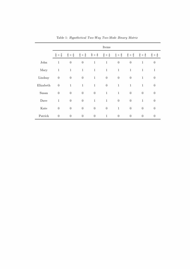
Table 1: Hypothetical Two-Way Two-Mode Binary Matrix

Items

5

9+ 7

9

2

3+ 1

2

3

4+ 5

6

6

7+ 4

7

3

8+ 1

8

1

4+ 2

3

2

5+ 3

4

3

5+ 4

5

2

3+ 4

8

John 1 0 0 1 1 0 0 1 0

Mary 1 1 1 1 1 1 1 1 1

Lindsay 0 0 0 1 0 0 0 1 0

Elizabeth 0 1 1 1 0 1 1 1 0

Susan 0 0 0 0 1 1 0 0 0

Dave 1 0 0 1 1 0 0 1 0

Kate 0 0 0 0 0 1 0 0 0

Patrick 0 0 0 0 1 0 0 0 0

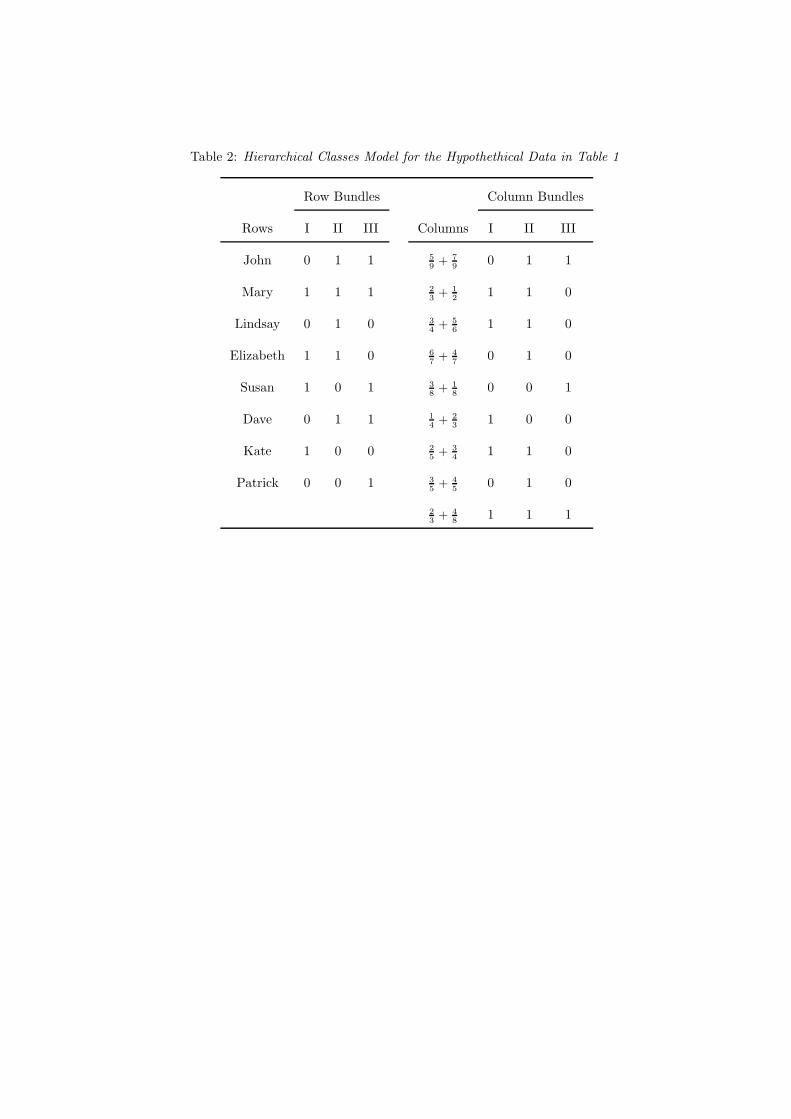
Table 2: Hierarchical Classes Model for the Hypothethical Data in Table 1

Row Bundles Column Bundles

Rows I II III Columns I II III

John 0 1 1 5

9+ 7

90 1 1

Mary 1 1 1 2

3+ 1

21 1 0

Lindsay 0 1 0 3

4+ 5

61 1 0

Elizabeth 1 1 0 6

7+ 4

70 1 0

Susan 1 0 1 3

8+ 1

80 0 1

Dave 0 1 1 1

4+ 2

31 0 0

Kate 1 0 0 2

5+ 3

41 1 0

Patrick 0 0 1 3

5+ 4

50 1 0

2

3+ 4

81 1 1