Lectures - School of Mathematics | The University of …sf/20912lectures01_19.pdfLectures Sergei...
119
Lectures Sergei Fedotov 20912 - Introduction to Financial Mathematics No tutorials in the first week Sergei Fedotov (University of Manchester) 20912 2010 1/1
Transcript of Lectures - School of Mathematics | The University of …sf/20912lectures01_19.pdfLectures Sergei...

Lectures
Sergei Fedotov
20912 - Introduction to Financial Mathematics
No tutorials in the first week
Sergei Fedotov (University of Manchester) 20912 2010 1 / 1

Lecture 1
1 IntroductionElementary economics backgroundWhat is financial mathematics?The role of SDE’s and PDE’s
2 Time Value of Money
3 Continuous Model for Stock Price
Sergei Fedotov (University of Manchester) 20912 2010 2 / 1
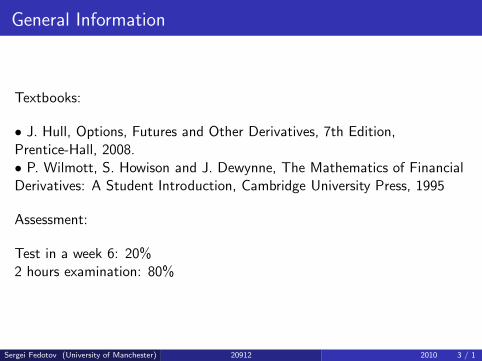
General Information
Textbooks:
• J. Hull, Options, Futures and Other Derivatives, 7th Edition,Prentice-Hall, 2008.• P. Wilmott, S. Howison and J. Dewynne, The Mathematics of FinancialDerivatives: A Student Introduction, Cambridge University Press, 1995
Assessment:
Test in a week 6: 20%2 hours examination: 80%
Sergei Fedotov (University of Manchester) 20912 2010 3 / 1

Elementary Economics Background
This course is concerned with mathematical models for financial markets:
• Stock Markets, such as NYSE(New York Stock Exchange), LondonStock Exchange, etc.
• Bond Markets, where participants buy and sell debt securities.
• Futures and Option Markets, where the derivative products are traded.
Example: European call option gives the holder the right (not obligation)to buy underlying asset at a prescribed time T for a specified price E .
Option market is massive! More money is invested in options than in theunderlying securities. The main purpose of this course is to determine theprice of options.
Why stochastic differential equations (SDE’s) and partial differentialequations (PDE’s)?
Sergei Fedotov (University of Manchester) 20912 2010 4 / 1

Time value of money
What is the future value V (t) at time t = T of an amount P invested orborrowed today at t = 0?
• Simple interest rate:V (T ) = (1 + rT )P (1)
where r > 0 is the simple interest rate, T is expressed in years.
• Compound interest rate:
V (T ) =(
1 +r
m
)mT
P (2)
where m is the number interest payments made per annum.
• Continuous compounding:In the limit m → ∞, we obtain
V (T ) = erT P (3)
since e = limz→∞(
1 + 1z
)z. Throughout this course the interest rate r
will be continuously compounded.Sergei Fedotov (University of Manchester) 20912 2010 5 / 1

Simple Model for Stock Price S(t)
Let S(t) represent the stock price at time t. How to write an equation forthis function?
• Return (relative measure of change):
∆S
S(4)
where ∆S = S(t + δt) − S(t)In the limit δt → 0 :
dS
S(5)
• How to model the return?Let us decompose the return into two parts: deterministic and stochastic
Sergei Fedotov (University of Manchester) 20912 2010 6 / 1

Modelling of Return
Return:
dS
S= µdt + σdW (6)
where µ is a measure of the expected rate of growth of the stock price. Ingeneral, µ = µ(S , t). In simpe models µ is taken to be constant(µ = 0.1 ÷ 0.3).
• σdW describes the stochastic change in the stock price, where dW
stands for∆W = W (t + ∆t)− W (t)
as ∆t → 0
• W (t) is a Wiener process
• σ is the volatility (σ = 0.2 ÷ 0.5)Sergei Fedotov (University of Manchester) 20912 2010 7 / 1

Stochastic differential equation for stock price
dS = µSdt + σSdW (7)
• Simple case: volatility σ = 0
dS = µSdt (8)
Sergei Fedotov (University of Manchester) 20912 2010 8 / 1

Wiener process
Definition. The standard Wiener process W (t) is a Gaussian process suchthat
• W (t) has independent increments: if u ≤ v ≤ s ≤ t, then W (t)− W (s)and W (v) − W (u) are independent
• W (s + t) − W (s) is N(0, t) and W (0) = 0
Clearly• EW (t) = 0 and EW 2 = t, where E is the expectation operator.
• The increment ∆W = W (t + ∆t) − W (t) can be written as
∆W = X (∆t)12 , where X is a random variable with normal distribution
with zero mean and unit variance:
X ∼ N (0, 1)
• E∆W = 0 and E(∆W )2 = ∆t.Sergei Fedotov (University of Manchester) 20912 2010 9 / 1

Lecture 2
1 Properties of Wiener Process
2 Approximation for Stock Price Equation
3 Ito’s Lemma
Sergei Fedotov (University of Manchester) 20912 2010 10 / 1

Wiener process
The probability density function for W (t) is
p(y , t) =1√2πt
exp
(
−y2
2t
)
and P (a ≤ W (t) ≤ b) =∫ b
ap(y , t)dy
• Simulations of a Wiener process:
Sergei Fedotov (University of Manchester) 20912 2010 11 / 1

Approximation of SDE for small ∆t
• The increment ∆W = W (t + ∆t) − W (t) can be written as
∆W = X (∆t)12 , where X is a random variable with normal distribution
with zero mean and unit variance: X ∼ N (0, 1)
• E∆W = 0 and E(∆W )2 = ∆t.Recall: equation for the stock price is
dS = µSdt + σSdW ,
then∆S ≈ µS∆t + σSX (∆t)
12
It means ∆S ∼ N(
µS∆t, σ2S2∆t)
Sergei Fedotov (University of Manchester) 20912 2010 12 / 1

Examples
Example 1. Consider a stock that has volatility 30% and provides expectedreturn of 15% p.a. Find the increase in stock price for one week if theinitial stock price is 100.
Answer: ∆S = 0.288 + 4.155X
Note: 4.155 is the standard deviation
Example 2. Show that the return ∆SS
is normally distributed with meanµ∆t and variance σ2∆t
Sergei Fedotov (University of Manchester) 20912 2010 13 / 1

Ito’s Lemma
We assume that f (S , t) is a smooth function of S and t.
Find df if dS = µSdt + σSdW
• Volatility σ = 0
df = ∂f∂t
dt + ∂f∂S
dS =(
∂f∂t
+ µS ∂f∂S
)
dt
• Volatility σ 6= 0
Ito’s Lemma:
df =(
∂f∂t
+ µS ∂f∂S
+ 12σ2S2 ∂2f
∂S2
)
dt + σS ∂f∂S
dW
Example. Find the SDE satisfied by f = S2.
Sergei Fedotov (University of Manchester) 20912 2010 14 / 1

Lecture 3
1 Distribution for lnS(t)
2 Solution to Stochastic Differential Equation for Stock Price
3 Examples
Sergei Fedotov (University of Manchester) 20912 2010 15 / 1

Differential of ln S
Example 1. Find the stochastic differential equation (SDE) for
f = lnS
by using Ito’s Lemma:
df =(
∂f∂t
+ µS ∂f∂S
+ 12σ2S2 ∂2f
∂S2
)
dt + σS ∂f∂S
dW
We obtain
df =
(
µ − σ2
2
)
dt + σdW
This is a constant coefficient SDE.
Integration from 0 to t gives
f − f0 =
(
µ − σ2
2
)
t + σW (t) since W (0) = 0.
Sergei Fedotov (University of Manchester) 20912 2010 16 / 1

Normal distribution for lnS(t)
We obtain for lnS(t)
lnS(t) − lnS0 =
(
µ − σ2
2
)
t + σW (t)
where S0 = S(0) is the initial stock price.
• lnS(t) has a normal distribution with mean lnS0 +(
µ − σ2
2
)
t and
variance σ2t.
Example 2. Consider a stock with an initial price of 40, an expected returnof 16% and a volatility of 20%.Find the probability distribution of lnS in six months.We have
lnS(T ) ∼ N
(
lnS0 +
(
µ − σ2
2
)
T , σ2T
)
Answer: lnS(0.5) ∼ N (3.759, 0.020)Sergei Fedotov (University of Manchester) 20912 2010 17 / 1

Probability density function for ln S(t)
Recall that if the random variable X has a normal distribution with meanµ and variance σ2, then the probability density function is
p(x) =1√
2πσ2exp
(
−(x − µ)2
2σ2
)
The probability density function of X = lnS(t) is
1√2πσ2t
exp
(
−(x − lnS0 − (µ − σ2/2)t)2
2σ2t
)
Sergei Fedotov (University of Manchester) 20912 2010 18 / 1

Exact expression for stock price S(t)
Definition. The model of a stock dS = µSdt + σSdW is known as ageometric Brownian motion.
The random function S(t) can be found from
ln(S(t)/S0) =
(
µ − σ2
2
)
t + σW (t)
Stock price at time t: S(t) = S0e
(
µ−σ2
2
)
t+σW (t)
Or
S(t) = S0e
(
µ−σ2
2
)
t+σ√
tXwhere X ∼ N (0, 1)
Sergei Fedotov (University of Manchester) 20912 2010 19 / 1

Lecture 4
1 Financial Derivatives
2 European Call and Put Options
3 Payoff Diagrams, Short Selling and Profit
Sergei Fedotov (University of Manchester) 20912 2010 20 / 1

Derivatives
• Derivative is a financial instrument which value depends on the values ofother underlying variables. Other names are financial derivative, derivativesecurity, derivative product. A stock option, for example, is a derivativewhose value is dependent on the stock price. Examples: forward contracts,futures, options, swaps, CDS, etc.• Options are very attractive to investors, both for speculation and forhedging
What is an Option?
Definition.European call option gives the holder the right (not obligation) to buyunderlying asset at a prescribed time T for a specified (strike) price E .
European put option gives its holder the right (not obligation) to sellunderlying asset at a prescribed time T for a specified (strike) price E .
The question is ”what does this actually mean?”Sergei Fedotov (University of Manchester) 20912 2010 21 / 1

Example.
Consider a three-month European call option on a BP share with a strikeprice E = 15 (T = 0.25). If you enter into this contract you have the rightbut not the obligation to buy one share for E = 15 in a three months time.
Whether you exercise your right depends on the stock price in the marketat time T :
• If the stock price is above £15, say £25, you can buy the share for £15,and sell it immediately for £25, making a profit of £10.
• If the stock price is below £15, there is no financial sense to buy it. Theoption is worthless.
Sergei Fedotov (University of Manchester) 20912 2010 22 / 1

Payoff Diagrams
We denote by C (S , t) the value of European call option and P(S , t) thevalue of European put option
Definition. Payoff Diagram ia a graph of the value of the option positionat expiration t = T as a function of the underlying stock price S .
Call price at t = T : C (S ,T ) = max (S − E , 0) =
{
0, S ≤ E ,S − E , S > E ,
Put price at t = T : P(S ,T ) = max (E − S , 0) =
{
E − S , S ≤ E ,0, S > E ,
If a trader thinks that the stock price is on the rise, he can make money bypurchase a call option without buying the stock. If a trader believes thestock price is on the decline, he can make money by buying put options.
Sergei Fedotov (University of Manchester) 20912 2010 23 / 1

Profit of call option buyer
The profit (gain) of a call option holder (buyer) at time T is
max (S − E , 0) − C0erT , C0 − initial call price
Example:Find the stock price on the exercise date in three months, for a Europeancall option with strike price £10 to give a gain (profit) of £14 if the optionis bought for £2.25, financed by a loan with continuously compoundedinterest rate of 5%
Solution:14 = S(T ) − 10 − 2.25 × e0.05× 1
4 ,
S(T ) = 26.28
For the holder of European put option, the profit at time T is
max (E − S , 0) − P0erT
.Sergei Fedotov (University of Manchester) 20912 2010 24 / 1

Portfolio and Short Selling
Definition. Short selling is the practice of selling assets that have beenborrowed from a broker with the intention of buying the same assets backat a later date to return to the broker.
This technique is used by investors who try to profit from the falling priceof a stock.
Definition. Portfolio is the combination of assets, options and bonds.
We denote by Π the value of portfolio. Example: Π = 2S + 4C − 5P .
It means that portfolio consists of long position in two shares, longposition in four call options and short position in five put options.
Sergei Fedotov (University of Manchester) 20912 2010 25 / 1

Option positions
Sergei Fedotov (University of Manchester) 20912 2010 26 / 1

Straddle
Straddle is the purchase of a call and a put on the same underlyingsecurity with the same maturity time T and strike price E .The value of portfolio is Π = C + P
• Straddle is effective when an investor is confident that a stock price willchange dramatically, but is uncertain of the direction of price move.
Example of large profits: S0 = 40, E = 40, C0 = 2, P0 = 2
Let us find an expected return!!Ans: 400
Sergei Fedotov (University of Manchester) 20912 2010 27 / 1
Lecture 5
1 Trading Strategies: Straddle, Bull Spread, etc.
2 Bond and Risk-Free Interest Rate
3 No Arbitrage Principle
Sergei Fedotov (University of Manchester) 20912 2010 28 / 1
Portfolio and Short Selling
Reminder from previous lecture 4.
Definition. Short selling is the practice of selling assets that have beenborrowed from a broker with the intention of buying the same assets backat a later date to return to the broker. This technique is used by investorswho try to profit from the falling price of a stock.
Definition. Portfolio is the combination of assets, options and bonds. Wedenote by Π the value of portfolio.
Examples.
Sergei Fedotov (University of Manchester) 20912 2010 29 / 1

Option positions
Sergei Fedotov (University of Manchester) 20912 2010 30 / 1

Trading Strategies Involving Options
Straddle is the purchase of a call and a put on the same underlyingsecurity with the same maturity time T and strike price E .
The value of portfolio is Π = C + P
• Straddle is effective when an investor is confident that a stock price willchange dramatically, but is uncertain of the direction of price move.
• Short Straddle, Π = −C − P , profits when the underlying securitychanges little in price before the expiration t = T .
Barings Bank was the oldest bank in London until its collapse in 1995. Ithappened when the bank’s trader, Nick Leeson, took short straddlepositions and lost 1.3 billion dollars.
Sergei Fedotov (University of Manchester) 20912 2010 31 / 1

Bull Spread
Bull spread is a strategy that is designed to profit from a moderate rise inthe price of the underlying security.
Let us set up a portfolio consisting of a long position in call with strikeprice E1and short position in call with E2 such that E1 < E2.
The value of this portfolio is Πt = Ct (E1) − Ct (E2). At maturity t = T
ΠT =
0, S ≤ E1,S − E1, E1 ≤ S < E2,
E2 − E1, S ≥ E2
• The holder of this portfolio benefits when the stock price will be aboveE1.
Sergei Fedotov (University of Manchester) 20912 2010 32 / 1

Risk-Free Interest Rate
We assume the existence of risk-free investment. Examples: USgovernment bond, deposit in a sound bank. We denote by B(t) the valueof this investment.
Definition. Bond is a contact that yields a known amount F , called theface value, on a known time T , called the maturity date. The authorizedissuer (for example, government) owes the holders a debt and is obliged topay interest (the coupon) and to repay the face value at maturity.
Zero-coupon bond involves only a single payment at T .Return dB
B= rdt, where r is the risk-free interest rate.
If B(T ) = F , then B(t) = Fe−r(T−t), where e−r(T−t) - discount factor
Sergei Fedotov (University of Manchester) 20912 2010 33 / 1

No Arbitrage Principle
The key principle of financial mathematics is No Arbitrage Principle.
• There are never opportunities to make risk-free profit• Arbitrage opportunity arises when a zero initial investment Π0 = 0 isidentified that guarantees non-negative payoff in the future such thatΠT > 0 with non-zero probability.
Arbitrage opportunities may exist in a real market. But, they cannot lastfor a long time.
Sergei Fedotov (University of Manchester) 20912 2010 34 / 1

Lecture 6
1 No-Arbitrage Principle
2 Put-Call Parity
3 Upper and Lower Bounds on Call Options
Sergei Fedotov (University of Manchester) 20912 2010 35 / 1

No Arbitrage Principle
The key principle of financial mathematics is No Arbitrage Principle.
• There are never opportunities to make risk-free profit.
• Arbitrage opportunity arises when a zero initial investment Π0 = 0 isidentified that guarantees non-negative payoff in the future such thatΠT > 0 with non-zero probability.Arbitrage opportunities may exist in a real market.
• All risk-free portfolios must have the same return: risk-free interest rate.Let Π be the value of a risk-free portfolio, and dΠ is its increment duringa small period of time dt. Then
dΠ
Π= rdt,
where r is the risk-less interest rate.• Let Πt be the value of the portfolio at time t. If ΠT ≥ 0, then Πt ≥ 0for t < T .
Sergei Fedotov (University of Manchester) 20912 2010 36 / 1

Put-Call Parity
Let us set up portfolio consisting of long one stock, long one put and shortone call with the same T and E .The value of this portfolio is Π = S + P − C .The payoff for this portfolio is
ΠT = S + max (E − S , 0) − max (S − E , 0) = E
The payoff is always the same whatever the stock price is at t = T .
Using No Arbitrage Principle, we obtain
St + Pt − Ct = Ee−r(T−t),
where Ct = C (St , t) and Pt = P (St , t).
This relationship between St ,Pt and Ct is called Put-Call Parity whichrepresents an example of complete risk elimination.
Sergei Fedotov (University of Manchester) 20912 2010 37 / 1

Upper and Lower Bounds on Call Options
• Put-Call Parity (t = 0): S0 + P0 − C0 = Ee−rT .
It shows that the value of European call option can be found from thevalue of European put option with the same strike price and maturity:
C0 = P0 + S0 − Ee−rT .
Therefore C0 ≥ S0 − Ee−rT since P0 ≥ 0 S0 − Ee−rT is the lower bound
for call option.
S0 − Ee−rT ≤ C0 ≤ S0
Let us illustrate these bounds geometrically.
Sergei Fedotov (University of Manchester) 20912 2010 38 / 1

Examples
Example 1. Find a lower bound for six months European call option withthe strike price £35 when the initial stock price is £40 and the risk-freeinterest rate is 5% p.a.
In this case S0 = 40, E = 35, T = 0.5, and r = 0.05.
The lower bound for the call option price is S0 − E exp (−rT ) , or
40 − 35 exp (−0.05 × 0.5) = 5.864
Example2. Consider the situation where the European call option is £4.Show that there exists an arbitrage opportunity.
We establish a zero initial investment Π0 = 0 by purchasing one call for£4 and the bond for £36 and selling one share for £40. The portfolio isΠ = C + B − S .
Sergei Fedotov (University of Manchester) 20912 2010 39 / 1

Examples
At maturity t = T , the portfolio Π = C + B − S has the value:
ΠT = max (S − E , 0) + 36 exp (0.05 × 0.5) − S =
{
36.911 − S , S ≤ 351.911 S > 35
It is clear that ΠT > 0, therefore there exists an arbitrage opportunity.
Sergei Fedotov (University of Manchester) 20912 2010 40 / 1

Lecture 7
1 Upper and Lower Bounds on Put Options
2 Proof of Put-Call Parity by No-Arbitrage Principle
3 Example on Arbitrage Opportunity
Sergei Fedotov (University of Manchester) 20912 2010 41 / 1

Upper and Lower Bounds on Put Option
Reminder from lecture 6.
• Arbitrage opportunity arises when a zero initial investment Π0 = 0 isidentified that guarantees a non-negative payoff in the future such thatΠT > 0 with non-zero probability.
• Put-Call Parity at time t = 0: S0 + P0 − C0 = Ee−rT .
Upper and Lower Bounds on Put Option (exercise sheet 3):
Ee−rT − S0 ≤ P0 ≤ Ee−rT
Let us illustrate these bounds geometrically.
Sergei Fedotov (University of Manchester) 20912 2010 42 / 1

Proof of Put-Call Parity
The value of European put option can be found as
P0 = C0 − S0 + Ee−rT .
Let us prove this relation by using No-Arbitrage Principle.
Assume that P0 > C0 − S0 + Ee−rT . Then one can make a riskless profit(arbitrage opportunity).
We set up the portfolio Π = −P − S + C + B . At time t = 0 we
• sell one put option for P0 (write the put option)
• sell one share for S0 (short position)
• buy one call option for C0
• buy one bond for B0 = P0 + S0 − C0 > Ee−rT
The balance of all these transactions is zero, that is, Π0 = 0Sergei Fedotov (University of Manchester) 20912 2010 43 / 1

Proof of Put-Call Parity
At maturity t = T the portfolio Π = −P − S + C + B has the value
ΠT =
{
−(E − S) − S + B0erT , S ≤ E ,
−S + (S − E ) + B0erT , S > E ,
= −E + B0erT
Since B0 > Ee−rT , we conclude ΠT > 0. and Π0 = 0.
This is an arbitrage opportunity.
Sergei Fedotov (University of Manchester) 20912 2010 44 / 1

Proof of Put-Call Parity
Now we assume that P0 < C0 − S0 + Ee−rT .
We set up the portfolio Π = P + S − C − B .
At time t = 0 we• buy one put option for P0
• buy one share for S0 (long position)
• sell one call option for C0 (write the call option)
• borrow B0 = P0 + S0 − C0 < Ee−rT
The balance of all these transactions is zero, that is, Π0 = 0
At maturity t = T we have ΠT = E − B0erT . Since B0 < Ee−rT , we
conclude ΠT > 0.
This is an arbitrage opportunity!!!Sergei Fedotov (University of Manchester) 20912 2010 45 / 1

Example on Arbitrage Opportunity
Three months European call and put options with the exercise price £12are trading at £3 and £6 respectively.The stock price is £8 and interest rate is 5%. Show that there existsarbitrage opportunity.
Solution:
The Put-Call Parity P0 = C0 − S0 + Ee−rT is violated, because
6 < 3 − 8 + 12e−0.05× 14 = 6.851
To get arbitrage profit we• buy a put option for £6• sell a call option for £3• buy a share for £8• borrow £11 at the interest rate 5%.The balance is zero!!
Sergei Fedotov (University of Manchester) 20912 2010 46 / 1

Example: Arbitrage Opportunity
The value of the portfolio Π = P + S − C − B at maturity T = 14 is
ΠT = E − B0erT = 12 − 11e0.05× 1
4 ≈ 0.862.
Combination P + S − C gives us £12. We repay the loan £11e0.05× 14 .
The balance 12 − 11e0.05× 14 is an arbitrage profit £0.862.
Sergei Fedotov (University of Manchester) 20912 2010 47 / 1
Lecture 8
1 One-Step Binomial Model for Option Price
2 Risk-Neutral Valuation
3 Examples
Sergei Fedotov (University of Manchester) 20912 2010 48 / 1

One-Step Binomial Model
Initial stock price is S0. The stock price can either move up from S0 toS0u or down from S0 to S0d ( u > 1; d < 1).
At time T , let the option price be Cu if the stock price moves up, and Cd
if the stock price moves down.
The purpose is to find the current price C0 of a European call option.Sergei Fedotov (University of Manchester) 20912 2010 49 / 1
Riskless Portfolio
Now, we set up a portfolio consisting of a long position in ∆ shares andshort position in one call
Π = ∆S − C
• Let us find the number of shares ∆ that makes the portfolio Π riskless.
The value of portfolio when stock moves up is
∆S0u − Cu
The value of portfolio when stock moves down is
∆S0d − Cd
If portfolio Π = ∆S − C is risk-free, then ∆S0u − Cu = ∆S0d − Cd
Sergei Fedotov (University of Manchester) 20912 2010 50 / 1

No-Arbitrage Argument
The number of shares is ∆ = Cu−Cd
S0(u−d) .
Because portfolio is riskless for this ∆, the current value Π0 can be foundby discounting: Π0 = (∆S0u − Cu) e−rT , where r is the interest rate.
On the other hand, the cost of setting up the portfolio is Π0 = ∆S0 − C0.Therefore ∆S0 − C0 = (∆S0u − Cu) e−rT .
Finally, the current call option price is
C0 = ∆S0 − (∆S0u − Cu) e−rT ,
where ∆ = Cu−Cd
S0(u−d) (No-Arbitrage Argument).
Sergei Fedotov (University of Manchester) 20912 2010 51 / 1

Risk-Neutral Valuation
AlternativelyC0 = e−rT (pCu + (1 − p)Cd) ,
where
p =erT − d
u − d.
(Risk-Neutral Valuation)
It is natural to interpret the variable 0 ≤ p ≤ 1 as the probability of an upmovement in the stock price, and the variable 1 − p as the probability of adown movement.
Fair price of a call option C0 is equal to the expected value of its futurepayoff discounted at the risk-free interest rate. For a put option P0 wehave the same result
P0 = e−rT (pPu + (1 − p)Pd) .
Sergei Fedotov (University of Manchester) 20912 2010 52 / 1

Example
A stock price is currently $40. At the end of three months it will be either$44 or $36. The risk-free interest rate is 12%.What is the value of three-month European call option with a strike priceof $42? Use no-arbitrage arguments and risk-neutral valuation.
In this case S0 = 40, u = 1.1, d = 0.9, r = 0.12, T = 0.25, Cu = 2,Cd = 0.
No-arbitrage arguments: the number of shares
∆ =Cu − Cd
S0u − S0d=
2 − 0
40 × (1.1 − 0.9)= 0.25
and the value of call option
C0 = S0∆ − (S0u∆ − Cu) e−rT =
40 × 0.25 − (40 × 1.1 × 0.25 − 2) × e−0.12×0.25 = 1.266
Sergei Fedotov (University of Manchester) 20912 2010 53 / 1

Example
Risk-neutral valuation: one can find the probability p
p =erT − d
u − d=
e0.12×0.25 − 0.9
1.1 − 0.9= 0.6523
and the value of call option
C0 = e−rT [pCu + (1 − p)Cd ] = e−0.12×0.25 [0.6523 × 2 + 0] = 1.266
Sergei Fedotov (University of Manchester) 20912 2010 54 / 1

Lecture 9
1 Risk-Neutral Valuation
2 Risk-Neutral World
3 Two-Steps Binomial Tree
Sergei Fedotov (University of Manchester) 20912 2010 55 / 1

Risk-Neutral Valuation
Reminder from Lecture 8. Call option price:
C0 = e−rT (pCu + (1 − p)Cd) ,
where p = erT−du−d
. No-Arbitrage Principle: d < erT < u.
In particular, if d > erT then there exists an arbitrage opportunity. Wecould make money by taking out a bank loan B0 = S0 at time t = 0 andbuying the stock for S0.
We interpret the variable 0 ≤ p ≤ 1 as the probability of an up movementin the stock price.
This formula is known as a risk-neutral valuation.
The probability of up q or down movement 1 − q in the stock price playsno role whatsoever! Why???
Sergei Fedotov (University of Manchester) 20912 2010 56 / 1

Risk Neutral Valuation
Let us find the expected stock price at t = T :
Ep [ST ] = pS0u + (1 − p)S0d = erT−du−d
S0u + (1 − erT−du−d
)S0d = S0erT .
This shows that stock price grows on average at the risk-free interest rater . Since the expected return is r , this is a risk-neutral world.
In Real World: E [ST ] = S0eµT . In Risk-Neutral World: Ep [ST ] = S0e
rT
Risk-Neutral Valuation: C0 = e−rTEp [CT ]
The option price is the expected payoff in a risk-neutral world, discountedat risk-free rate r .
Sergei Fedotov (University of Manchester) 20912 2010 57 / 1
Two-Step Binomial Tree
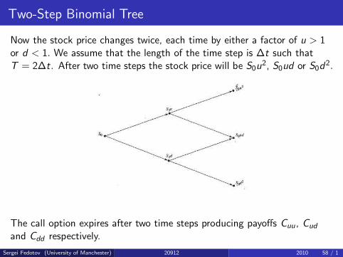
Now the stock price changes twice, each time by either a factor of u > 1or d < 1. We assume that the length of the time step is ∆t such thatT = 2∆t. After two time steps the stock price will be S0u
2, S0ud or S0d2.
The call option expires after two time steps producing payoffs Cuu, Cud
and Cdd respectively.
Sergei Fedotov (University of Manchester) 20912 2010 58 / 1

Option Price
The purpose is to calculate the option price C0 at the initial node of thetree.We apply the risk-neutral valuation backward in time:Cu = e−r∆t (pCuu + (1 − p)Cud) , Cd = e−r∆t (pCud + (1 − p)Cdd) .
Current option price: C0 = e−r∆t (pCu + (1 − p)Cd) .
Sergei Fedotov (University of Manchester) 20912 2010 59 / 1

Option Price
Substitution gives
C0 = e−2r∆t(
p2Cuu + 2p(1 − p)Cud + (1 − p)2Cdd
)
,
where p2, 2p(1 − p) and (1 − p)2 are the probabilities in a risk-neutralworld that the upper, middle, and lower final nodes are reached.
Finally, the current call option price is
C0 = e−rTEp [CT ] , T = 2∆t.
The current put option price can be found in the same way:
P0 = e−2r∆t(
p2Puu + 2p(1 − p)Pud + (1 − p)2Pdd
)
orP0 = e−rT
Ep [PT ] .
Sergei Fedotov (University of Manchester) 20912 2010 60 / 1

Two-Step Binomial Tree Example
Consider six months European put with a strike price of £32 on a stockwith current price £40. There are two time steps and in each time stepthe stock price either moves up by 20% or moves down by 20%. Risk-freeinterest rate is 10%. Find the current option price.
We have u = 1.2, d = 0.8, ∆t = 0.25, and r = 0.1.Risk-neutral probability p = er∆t−d
u−d= e0.1×0.25−0.8
1.2−0.8 = 0.5633.
The possible stock prices at final nodes are 40 × (1.2)2 = 57.6,40 × 1.2 × 0.8 = 38.4, and 40 × (0.8)2 = 25.6.
We obtain Puu = 0, Pud = 0 and Pdd = 32 − 25.6 = 6.4.
Thus the value of put option is
P0 = e−2×0.1×0.25 ×(
0 + 0 + (1 − 0.5633)2 × 6.4)
= 1.1610.
Sergei Fedotov (University of Manchester) 20912 2010 61 / 1

Lecture 10
1 Binomial Model for Stock Price
2 Option Pricing on Binomial Tree
3 Matching Volatility σ with u and d
Sergei Fedotov (University of Manchester) 20912 2010 62 / 1

Binomial model for the stock price
Continuous random model for the stock price: dS = µSdt + σSdW
The binomial model for the stock price is a discrete time model:
• The stock price S changes only at discrete times ∆t, 2∆t, 3∆t, ...
• The price either moves up S → Su or down S → Sd with d < er∆t < u.
• The probability of up movement is q.
Let us build up a tree of possible stock prices. The tree is called a binomialtree, because the stock price will either move up or down at the end ofeach time period. Each node represents a possible future stock price.
We divide the time to expiration T into several time steps of duration∆t = T/N, where N is the number of time steps in the tree.
Example: Let us sketch the binomial tree for N = 4.Sergei Fedotov (University of Manchester) 20912 2010 63 / 1

Stock Price Movement in the Binomial Model
We introduce the following notations:
• Smn is the n-th possible value of stock price at time-step m∆t.
Then Smn = undm−nS0
0 , where n = 0, 1, 2, ...,m.
S00 is the stock price at the time t = 0. Note that u and d are the same at
every node in the tree.
For example, at the third time-step 3∆t, there are four possible stockprices: S3
0 = d3S00 , S3
1 = ud2S00 , S3
2 = u2dS00 and S3
3 = u3S00 .
At the final time-step N∆t, there are N + 1 possible values of stock price.
Sergei Fedotov (University of Manchester) 20912 2010 64 / 1

Call Option Pricing on Binomial Tree
We denote by Cmn the n-th possible value of call option at time-step m∆t.
• Risk Neutral Valuation (backward in time):
Cmn = e−r∆t
(
pCm+1n+1 + (1 − p)Cm+1
n
)
.
Here 0 ≤ n ≤ m and p = er∆t−du−d
.
• Final condition: CNn = max
(
SNn − E , 0
)
, where n = 0, 1, 2, ...,N, E is the
strike price.
The current option price C 00 is the expected payoff in a risk-neutral world,
discounted at risk-free rate r : C 00 = e−rT
Ep [CT ] .
Example: N = 4.
Sergei Fedotov (University of Manchester) 20912 2010 65 / 1

Matching volatility σ with u and d
We assume that the stock price starts at the value S0 and the time step is∆t. Let us find the expected stock price, E [S ] , and the variance of thereturn, var
[
∆SS
]
, for continuous and discrete models.
• Expected stock price: Continuous model: E [S ] = S0eµ∆t .
On the binomial tree: E [S ] = qS0u + (1 − q)S0d .
First equation: qu + (1 − q)d = eµ∆t .
• Variance of the return: Continuous model: var[
∆SS
]
= σ2∆t (Lecture2)
On the binomial tree: var[
∆SS
]
=
q(u − 1)2 + (1 − q)(d − 1)2 − [q(u − 1) + (1 − q)(d − 1)]2 =qu2 + (1 − q)d2 − [qu + (1 − q)d ]2 .
Recall: var [X ] = E[
X 2]
− [E (X )]2.
Second equation: qu2 + (1 − q)d2 − [qu + (1 − q)d ]2 = σ2∆t.Third equation: u = d−1.
Sergei Fedotov (University of Manchester) 20912 2010 66 / 1

Matching volatility σ with u and d
From the first equation we find q = eµ∆t−du−d
.
This is the probability of an up movement in the real world.
Substituting this probability into the second equation, we obtain
eµ∆t(u + d) − ud − e2µ∆t = σ2∆t.
Using u = d−1, we get
eµ∆t(u +1
u) − 1 − e2µ∆t = σ2∆t.
This equation can be reduced to the quadratic equation. (Exercise sheet 4,part 5).
One can obtain u ≈ eσ√
∆t ≈ 1 + σ√
∆t and d ≈ e−σ√
∆t .
These are the values of u and d obtained by Cox, Ross, and Rubinstein in1979.
Recall: ex ≈ 1 + x for small x .Sergei Fedotov (University of Manchester) 20912 2010 67 / 1

Lecture 11
1 American Put Option Pricing on Binomial Tree
2 Replicating Portfolio
Sergei Fedotov (University of Manchester) 20912 2010 68 / 1

American Option
• An American Option is one that may be exercised at any time prior toexpire (t = T ).
• We should determine when it is best to exercise the option.
• It is not subjective! It can be determined in a systematic way!
• The American put option value must be greater than or equal to thepayoff function.
If P < max(E − S , 0), then there is obvious arbitrage opportunity.
We can buy stock for S and option for P and immediately exercise theoption by selling stock for E .E − (P + S) > 0
Sergei Fedotov (University of Manchester) 20912 2010 69 / 1

American Put Option Pricing on Binomial Tree
We denote by Pmn the n-th possible value of put option at time-step m∆t.
• European Put Option:
Pmn = e−r∆t
(
pPm+1n+1 + (1 − p)Pm+1
n
)
.
Here 0 ≤ n ≤ m and the risk-neutral probability p = er∆t−du−d
.
• American Put Option:
Pmn = max
{
max(E − Smn , 0), e−r∆t
(
pPm+1n+1 + (1 − p)Pm+1
n
)
}
,
where Smn is the n-th possible value of stock price at time-step m∆t.
• Final condition: PNn = max
(
E − SNn , 0
)
, where n = 0, 1, 2, ...,N, E is the
strike price.
Sergei Fedotov (University of Manchester) 20912 2010 70 / 1
Example: Evaluation of American Put Option on Two-Step
Tree
We assume that over each of the next two years the stock price eithermoves up by 20% or moves down by 20%. The risk-free interest rate is 5%.
Find the value of a 2-year American put with a strike price of $52 on astock whose current price is $50.
In this case u = 1.2, d = 0.8, r = 0.05, E = 52.
Risk-neutral probability: p = e0.05−0.81.2−0.8 = 0.6282
Sergei Fedotov (University of Manchester) 20912 2010 71 / 1

Replicating Portfolio
The aim is to calculate the value of call option C0.
Let us establish a portfolio of stocks and bonds in such a way that thepayoff of a call option is completely replicated.
Final value: ΠT = CT = max (S − E , 0)
To prevent risk-free arbitrage opportunity, the current values should beidentical. We say that the portfolio replicates the option.
The Law of One Price: Πt = Ct .
Consider replicating portfolio of ∆ shares held long and N bonds heldshort.The value of portfolio: Π = ∆S − NB . A pair (∆,N) is called a tradingstrategy.
How to find (∆,N) such that ΠT = CT and Π0 = C0?Sergei Fedotov (University of Manchester) 20912 2010 72 / 1

Example: One-Step Binomial Model.
Initial stock price is S0. The stock price can either move up from S0 toS0u or down from S0 to S0d . At time T , let the option price be Cu if thestock price moves up, and Cd if the stock price moves down.
The value of portfolio: Π = ∆S − NB .
When stock moves up: ∆S0u − NB0erT = Cu.
When stock moves down: ∆S0d − NB0erT = Cd .
We have two equations for two unknown variables ∆ and N.
Current value: C0 = ∆S0 − NB0.
Prove: C0 = e−rT (pCu + (1 − p)Cd) , where p = erT−du−d
. (Exercise sheet 5)
Sergei Fedotov (University of Manchester) 20912 2010 73 / 1

Lecture 12
1 Black-Scholes Model
2 Black-Scholes Equation
The Black-Scholes model for option pricing was developed by FischerBlack, Myron Scholes in the early 1970s. This model is the mostimportant result in financial mathematics.
Sergei Fedotov (University of Manchester) 20912 2010 74 / 1

Black - Scholes model
The Black-Scholes model is used to calculate an option price using: stockprice S , strike price E , volatility σ, time to expiration T , and risk-freeinterest rate r .
This model involves the following explicit assumptions:
• The stock price follows a Geometric Brownian motion with constantexpected return and volatility: dS = µSdt + σSdW . .
• No transaction costs.
• The stock does not pay dividends.
• One can borrow and lend cash at a constant risk-free interest rate.
• Securities are perfectly divisible (i.e. one can buy any fraction of a shareof stock).
• No restrictions on short selling.Sergei Fedotov (University of Manchester) 20912 2010 75 / 1

Basic Notation
We denote by V (S , t) the value of an option. We use the notationsC (S , t) and P(S , t) for call and put when the distinction is important.
• The aim is to derive the famous Black-Scholes Equation:
∂V
∂t+
1
2σ2S2 ∂2V
∂S2+ rS
∂V
∂S− rV = 0.
Now, we set up a portfolio consisting of a long position in one option anda short position in ∆ shares.
The value is Π = V − ∆S .
• Let us find the number of shares ∆ that makes this portfolio riskless.
Sergei Fedotov (University of Manchester) 20912 2010 76 / 1

Ito’s Lemma and Elimination of Risk
The change in the value of this portfolio in the time interval dt:dΠ = dV − ∆dS , where dS = µSdt + σSdW .
Using Ito’s Lemma:
dV =
(
∂V
∂t+
1
2σ2S2 ∂2V
∂S2+ µS
∂V
∂S
)
dt + σS∂V
∂SdW ,
we find
dΠ =
(
∂V
∂t+
1
2σ2S2 ∂2V
∂S2+ µS
∂V
∂S− µS∆
)
dt +
(
σS∂V
∂S− ∆σS
)
dW .
The main question is how to eliminate the risk!!!
We can eliminate the random component in dΠ by choosing ∆ = ∂V∂S
.
Sergei Fedotov (University of Manchester) 20912 2010 77 / 1

Black-Scholes Equation
This choice results in a risk-free portfolio Π = V − S ∂V∂S
whose increment
is dΠ =(
∂V∂t
+ 12σ2S2 ∂2V
∂S2
)
dt.
• No-Arbitrage Principle: the return from this portfolio must be rdt.
dΠΠ = rdt or
∂V∂t
+ 12σ2S2 ∂2V
∂S2
V−S ∂V∂S
= r or ∂V∂t
+ 12σ2S2 ∂2V
∂S2 = r(
V − S ∂V∂S
)
.
Thus, we obtain the Black-Scholes PDE:
∂V
∂t+
1
2σ2S2 ∂2V
∂S2+ rS
∂V
∂S− rV = 0.
Scholes received the 1997 Nobel Prize in Economics. It was not awardedto Black in 1997, because he died in 1995.Black received a Ph.D. in applied mathematics from Harvard University.
Sergei Fedotov (University of Manchester) 20912 2010 78 / 1

The European call value C (S , t)
If PDE is of backward type, we must impose a final condition at t = T .For a call option, we have C (S ,T ) = max(S − E , 0).
Sergei Fedotov (University of Manchester) 20912 2010 79 / 1

Lecture 13
1 Boundary Conditions for Call and Put Options
2 Exact Solution to Black-Scholes Equation
∂C
∂t+
1
2σ2S2 ∂2C
∂S2+ rS
∂C
∂S− rC = 0.
Sergei Fedotov (University of Manchester) 20912 2010 80 / 1

Boundary Conditions
We use C (S , t) and P(S , t) for call and put option. Boundary conditionsare applied for zero stock price S = 0 and S → ∞.
• Boundary conditions for a call option:
C (0, t) = 0 and C (S , t) → S as S → ∞.
The call option is likely to be exercised as S → ∞
• Boundary conditions for a put option:
P(0, t) = Ee−r(T−t). We evaluate the present value of E .
P(S , t) → 0 as S → ∞.As stock price S → ∞, then put option is unlikely to be exercised.
Sergei Fedotov (University of Manchester) 20912 2010 81 / 1

Exact solution
The Black-Scholes equation
∂C
∂t+
1
2σ2S2 ∂2C
∂S2+ rS
∂C
∂S− rC = 0
with appropriate final and boundary conditions has the explicit solution:
C (S , t) = SN (d1) − Ee−r(T−t)N (d2) ,
where
N (x) =1√2π
∫ x
−∞e−
y2
2 dy (cumulative normal distribution)
and
d1 =ln (S/E ) +
(
r + σ2/2)
(T − t)
σ√
T − t, d2 = d1 − σ
√T − t.
Sergei Fedotov (University of Manchester) 20912 2010 82 / 1

The European call value C (S , t) by K. Rubash
Sergei Fedotov (University of Manchester) 20912 2010 83 / 1

Example
Calculate the price of a three-month European call option on a stock witha strike price of $25 when the current stock price is $21.6 The volatility is35% and risk-free interest rate is 1% p.a.
In this case S0 = 21.6,E = 25,T = 0.25, σ = 0.35 and r = 0.01.
The value of call option is C0 = S0N (d1) − Ee−rT N (d2) .
First, we compute the values of d1 and d2:
d1 =ln(S0/E)+(r+σ2/2)T
σ√
T=
ln( 21.625 )+(0.01+(0.35)2×0.5))×0.25
0.35×√
0.25≈ −0.7335
d2 = d1 − σ√
T = −0.7335 − 0.35 ×√
0.25 ≈ −0.9085
SinceN (−0.7335) ≈ 0.2316, N (−0.9085) ≈ 0.1818,
we obtain
C0 ≈ 21.6 × 0.2316 − 25 × e−0.01×0.25 × 0.1818 = 0.4689Sergei Fedotov (University of Manchester) 20912 2010 84 / 1

The Limit of Higher Volatility
Let us find the limit
limσ→∞
C (S , t).
We know that
C (S , t) = SN (d1) − Ee−r(T−t)N (d2) ,
where d1 =ln(S/E)+(r+σ2/2)(T−t)
σ√
T−t= ln(S/E)
σ√
T−t+ r
√T−tσ + σ
√T−t2 .
In the limit σ → ∞, d1 → ∞.
Since d2 = d1 − σ√
T − t, in the limit σ → ∞, d2 → −∞
Thus limσ→∞ N (d1) = 1 and limσ→∞ N(d2) = 0.
Therefore limσ→∞ C (S , t) = S . This is an upper bound for call option!!!
Sergei Fedotov (University of Manchester) 20912 2010 85 / 1

Lecture 14
1 ∆-Hedging
2 Greek Letters or Greeks
Sergei Fedotov (University of Manchester) 20912 2010 86 / 1
Delta for European Call Option
Let us show that ∆ = ∂C∂S
= N (d1) .
First, find the derivative ∆ = ∂C∂S
by using the explicit solution for the
European call C (S , t) = SN (d1) − Ee−r(T−t)N (d2).
∆ =∂C
∂S= N (d1) + SN ′ (d1)
∂d1
∂S− Ee−r(T−t)N ′ (d2)
∂d2
∂S=
N (d1) + (SN ′ (d1) − Ee−r(T−t)N ′ (d2))∂d1
∂S.
We need to prove
(SN ′ (d1) − Ee−r(T−t)N ′ (d2)) = 0.
See Problem Sheet 6.
Sergei Fedotov (University of Manchester) 20912 2010 87 / 1

Delta-Hedging Example
Find the value of ∆ of a 6-month European call option on a stock with astrike price equal to the current stock price ( t = 0). The interest rate is6% p.a. The volatility σ = 0.16.
Solution: we have ∆ = N (d1) , where d1 =ln(S0/E)+(r+σ2/2)T
σ(T )12
We find
d1 =(0.06 + (0.16)2 × 0.5)) × 0.5
0.16 ×√
0.5≈ 0.3217
and∆ = N (0.3217) ≈ 0.6262
Sergei Fedotov (University of Manchester) 20912 2010 88 / 1

Delta for European Put Option
Let us find Delta for European put option by using the put-call parity:
S + P − C = Ee−r(T−t).
Let us differentiate it with respect to S
We find 1 + ∂P∂S
− ∂C∂S
= 0.
Therefore ∂P∂S
= ∂C∂S
− 1 = N (d1) − 1.
Sergei Fedotov (University of Manchester) 20912 2010 89 / 1

Greeks
The option value: V = V (S , t | σ, r ,T ).
Greeks represent the sensitivities of options to a change in underlyingparameters on which the value of an option is dependent.
• Delta:
∆ = ∂V∂S
measures the rate of change of option value with respect tochanges in the underlying stock price
• Gamma:
Γ = ∂2V∂S2 = ∂∆
∂Smeasures the rate of change in ∆ with respect to changes
in the underlying stock price.
Problem Sheet 6: Γ = ∂2C∂S2 = N′(d1)
Sσ√
T−t, where N ′(d1) = 1√
2πe−
d212 .
Sergei Fedotov (University of Manchester) 20912 2010 90 / 1

Greeks
• Vega, ∂V∂σ , measures sensitivity to volatility σ.
One can show that ∂C∂σ = S
√T − tN ′(d1).
• Rho:
ρ = ∂V∂r
measures sensitivity to the interest rate r .
One can show that ρ = ∂C∂r
= E (T − t)e−r(T−t)N(d2).
The Greeks are important tools in financial risk management. Each Greekmeasures the sensitivity of the value of derivatives or a portfolio to a smallchange in a given underlying parameter.
Sergei Fedotov (University of Manchester) 20912 2010 91 / 1

Lecture 15
1 Black-Scholes Equation and Replicating Portfolio
2 Static and Dynamic Risk-Free Portfolio
Sergei Fedotov (University of Manchester) 20912 2010 92 / 1
Replicating Portfolio
The aim is to show that the option price V (S , t) satisfies theBlack-Scholes equation
∂V
∂t+
1
2σ2S2 ∂2V
∂S2+ rS
∂V
∂S− rV = 0.
Consider replicating portfolio of ∆ shares held long and N bonds heldshort. The value of portfolio: Π = ∆S − NB . Recall that a pair (∆,N) iscalled a trading strategy.
How to find (∆,N) such that Πt = Vt?
• SDE for a stock price S(t) : dS = µSdt + σSdW .
• Equation for a bond price B (t) : dB = rBdt.
Sergei Fedotov (University of Manchester) 20912 2010 93 / 1

Derivation of the Black-Scholes Equation
By using the Ito’s lemma, we find the change in the option value
dV =
(
∂V
∂t+ µS
∂V
∂S+
1
2σ2S2 ∂2V
∂S2
)
dt + σS∂V
∂SdW .
By using self-financing requirement dΠ = ∆dS −NdB , we find the changein portfolio value
dΠ = ∆dS−NdB = ∆(µSdt+σSdW )−rNBdt = (∆µS−rNB)dt+∆σSdW
Equating the last two equations dΠ = dV , we obtain
∆ = ∂V∂S
, −rNB = ∂V∂t
+ 12σ2S2 ∂2V
∂S2 .
Since NB = ∆S − Π =(
S ∂V∂S
− V)
, we get the classical Black-Scholesequation
∂V
∂t+
1
2σ2S2 ∂2V
∂S2+ rS
∂V
∂S− rV = 0.
Sergei Fedotov (University of Manchester) 20912 2010 94 / 1

Static Risk-free Portfolio
Let me remind you a Put-Call Parity. We set up the portfolio consisting oflong position in one stock, long position in one put and short position inone call with the same T and E .The value of this portfolio is Π = S + P − C .The payoff for this portfolio is
ΠT = S + max (E − S , 0) − max (S − E , 0) = E
The payoff is always the same whatever the stock price is at t = T .
Using No Arbitrage Principle, we obtain
St + Pt − Ct = Ee−r(T−t),
where Ct = C (St , t) and Pt = P (St , t).
This is an example of complete risk elimination.
Definition: The risk of a portfolio is the variance of the return.Sergei Fedotov (University of Manchester) 20912 2010 95 / 1

Dynamic Risk-Free Portfolio
Put-Call Parity is an example of complete risk elimination when we carryout only one transaction in call/put options and underlying security.
Let us consider the dynamic risk elimination procedure.
We could set up a portfolio consisting of a long position in one call optionand a short position in ∆ shares.
The value is Π = C − ∆S .
We can eliminate the random component in Π by choosing
∆ =∂C
∂S.
This is a ∆-hedging! It requires a continuous rebalancing of a number ofshares in the portfolio Π.
Sergei Fedotov (University of Manchester) 20912 2010 96 / 1

Lecture 16
1 Option on Dividend-paying Stock
2 American Put Option
Sergei Fedotov (University of Manchester) 20912 2010 97 / 1

Option on Dividend-paying Stock
We assume that in a time dt the underlying stock pays out a dividend
D0Sdt,
where D0 is a constant dividend yield.
Now, we set up a portfolio consisting of a long position in one call optionand a short position in ∆ shares.
The value is Π = C − ∆S .
The change in the value of this portfolio in the time interval dt:
dΠ = dC − ∆dS − ∆D0Sdt.
Sergei Fedotov (University of Manchester) 20912 2010 98 / 1

Ito’s Lemma and Elimination of Risk
Using Ito’s Lemma:
dC =
(
∂C
∂t+
1
2σ2S2 ∂2C
∂S2
)
dt +∂C
∂SdS
we find
dΠ =
(
∂C
∂t+
1
2σ2S2 ∂2C
∂S2− D0S
∂C
∂S
)
dt +∂C
∂SdS − ∆dS
We can eliminate the random component in dΠ by choosing ∆ = ∂C∂S
.
Sergei Fedotov (University of Manchester) 20912 2010 99 / 1

Modified Black-Scholes Equation
This choice results in a risk-free portfolio Π = C − S ∂C∂S
whose increment
is dΠ =(
∂C∂t
+ 12σ2S2 ∂2C
∂S2 − D0S∂C∂S
)
dt.
• No-Arbitrage Principle: the return from this portfolio must be rdt.
dΠΠ = rdt or ∂C
∂t+ 1
2σ2S2 ∂2C∂S2 − D0S
∂C∂S
= r(
C − S ∂C∂S
)
.
Thus, we obtain the modified Black-Scholes PDE:
∂C
∂t+
1
2σ2S2 ∂2C
∂S2+ (r − D0)S
∂C
∂S− rC = 0.
Sergei Fedotov (University of Manchester) 20912 2010 100 / 1

Solution to Modified Black-Scholes Equation
Let us find the solution to modified Black-Scholes equation in the form
C (S , t) = e−D0(T−t)C1(S , t).
We prove that C1(S , t) satisfies the Black-Scholes equation with r
replaced by r − D0.
If we substitute C (S , t) = e−D0(T−t)C1(S , t) into the modifiedBlack-Scholes equation, we find the equation for C1(S , t) in the form
∂C1
∂t+
1
2σ2S2 ∂2C1
∂S2+ (r − D0)
∂C1
∂S− (r − D0)C1 = 0
. The auxiliary function C1(S , t) is the value of a European Call optionwith the interest rate r − D0.
Sergei Fedotov (University of Manchester) 20912 2010 101 / 1

Solution to Modified Black-Scholes Equation
Problem sheet 7: show that the modified Black-Scholes equation has theexplicit solution for the European call
C (S , t) = Se−D0(T−t)N (d10) − Ee−r(T−t)N (d20) ,
where
d10 =ln (S/E ) +
(
r − D0 + σ2/2)
(T − t)
σ√
T − t, d20 = d10 − σ
√T − t.
Sergei Fedotov (University of Manchester) 20912 2010 102 / 1

American Put Option
Recall that An American Option is one that may be exercised at any timeprior to expire (t = T ).
• The American put option value must be greater than or equal to thepayoff function.
If P < max(E − S , 0), then there is obvious arbitrage opportunity.
Sergei Fedotov (University of Manchester) 20912 2010 103 / 1

American Put Option
American put problem can be written as as a free boundary problem.
We divide the price axis S into two distinct regions:
0 ≤ S < Sf (t) and Sf (t) < S < ∞,
where Sf (t) is the exercise boundary. Note that we do not know a priorithe value of Sf (t).
When 0 ≤ S < Sf (t), the early exercise is optimal: put option value isP(S , t) = E − S .
When S > Sf (t), the early exercise is not optimal, and P(S , t) obeys theBlack-Scholes equation.
The boundary conditions at S = Sf (t) are
P (Sf (t), t) = max (E − Sf (t), 0) ,∂P
∂S(Sf (t), t) = −1.
Sergei Fedotov (University of Manchester) 20912 2010 104 / 1
Lecture 17
1 Bond Pricing with Known Interest Rates and Dividend Payments
2 Zero-Coupon Bond Pricing
Sergei Fedotov (University of Manchester) 20912 2010 105 / 1

Bond Pricing Equation
• Definition. A bond is a contract that yields a known amount (nominal,principal or face value) on the maturity date, t = T . The bond pays thedividends at fixed times.
If there is no dividend payment, the bond is known as a zero-coupon bond.
Let us introduce the following notation
V (t) is the value of the bond, r(t) is the interest rate, K (t) is thecoupon payment.
Equation for the bond price is
dV
dt= r(t)V − K (t).
The final condition: V (T ) = F .
Sergei Fedotov (University of Manchester) 20912 2010 106 / 1

Zero-Coupon Bond Pricing
Let us consider the case when the dividend payment K (t) = 0.
The solution of the equation dVdt
= r(t)V with V (T ) = F can be writtenas
V (t) = F exp
(
−∫ T
t
r(s)ds
)
.
Let us show this by integration dVV
= r(t)dt from t to T .
lnV (T ) − lnV (t) =∫ T
tr(s)ds or ln(V (t)/F ) = −
∫ T
tr(s)ds.
Sergei Fedotov (University of Manchester) 20912 2010 107 / 1

Example
A zero coupon bond, V , issued at t = 0, is worth V (1) = 1 at t = 1. Findthe bond price V (t) at time t < 1 and V (0), when the continuous interestrate is
r(t) = t2.
Solution: T = 1; one can find
∫ 1
t
r(s)ds =
∫ 1
t
s2ds =1
3− 1
3t3
Therefore
V (t) = exp
(
−∫ 1
t
r(s)ds
)
= exp
(
t3
3− 1
3
)
,
V (0) = exp
(
−1
3
)
= 0.7165
Sergei Fedotov (University of Manchester) 20912 2010 108 / 1

Bond Pricing for K (t) > 0
Let us consider the case when the dividend payment K (t) > 0. Thesolution of the equation dV
dt= r(t)V − K (t) can be written as
V (t) = F exp
(
−∫ T
t
r(s)ds
)
+ V1 (t) ,
where V1 (t) = C (t) exp(
−∫ T
tr(s)ds
)
.
To find C (t) we need to substitute V1 (t) into the equation
dV1
dt= r(t)V1 − K (t).
(tutorial exercise 8)
The explicit solution is
V (t) = exp
(
−∫ T
t
r(s)ds
) [
F +
∫ T
t
K (y) exp
(∫ T
y
r(s)ds
)
dy
]
.
Sergei Fedotov (University of Manchester) 20912 2010 109 / 1

Lecture 18
1 Measure of Future Values of Interest Rate
2 Term Structure of Interest Rate (Yield Curve)
Sergei Fedotov (University of Manchester) 20912 2010 110 / 1

Measure of Future Value of Interest Rate
Let us consider the case when the dividend payment K (t) = 0. Recall thatthe solution of the equation dV
dt= r(t)V with V (T ) = F is
V (t) = F exp
(
−∫ T
t
r(s)ds
)
.
Let us introduce the notation V (t,T ) for the bond prices. These pricesare quoted at time t for different values of T .
Let us differentiate V (t,T ) with respect to T :
∂V∂T
= F exp(
−∫ T
tr(s)ds
)
(−r(T )) = −V (t,T )r(T ),
since ∂∂T
∫ T
tr(s)ds = r(T ). Therefore,
r(T ) = − 1
V (t,T )
∂V
∂T.
This is an interest rate at future dates (forward rate).Sergei Fedotov (University of Manchester) 20912 2010 111 / 1

Term Structure of Interest Rate (Yield Curve)
We define
Y (t,T ) = − ln(V (t,T )) − lnV (T ,T )
T − t
as a measure of the future values of interest rate, where V (t,T ) is takenfrom financial data.
Y (t,T ) = −ln(F exp
(
−∫ Tt
r(s)ds)
)−ln F
T−t= 1
T−t
∫ T
tr(s)ds
is the average value of the interest rate r(t) in the time interval [t,T ].
Bond price V (t,T ) can be written as V (t,T ) = Fe−Y (t,T )(T−t).
Term structure of interest rate (yield curve):
Y (0,T ) = − ln(V (0,T )) − lnV (T ,T )
T=
1
T
∫ T
0r(s)ds
is the average value of interest rate in the future.Sergei Fedotov (University of Manchester) 20912 2010 112 / 1
Example
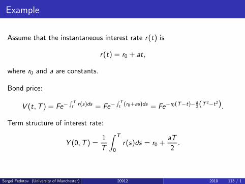
Assume that the instantaneous interest rate r(t) is
r(t) = r0 + at,
where r0 and a are constants.
Bond price:
V (t,T ) = Fe−∫ T
tr(s)ds = Fe−
∫ T
t(r0+as)ds = Fe−r0(T−t)− a
2(T2−t2).
Term structure of interest rate:
Y (0,T ) =1
T
∫ T
0r(s)ds = r0 +
aT
2.
Sergei Fedotov (University of Manchester) 20912 2010 113 / 1

Risk of Default
There exists a risk of default of bond V (t) when the principal are not paidto the lender as promised by borrower.
How to take this into account?
Let us introduce the probability of default p during one year T = 1. Then
V (0) er = V (0) (1 − p)e(r+s) + p × 0.
The investor has no preference between two investments.The positive parameter s is called the spread w.r.t to interest rate r .
Let us find it.s = − ln(1 − p) = p + o(p).
Sergei Fedotov (University of Manchester) 20912 2010 114 / 1

Lecture 19
1 Asian Options
2 Derivation of PDE for Option Price
Sergei Fedotov (University of Manchester) 20912 2010 115 / 1

Asian Options
• Definition. Asian option is a contract giving the holder the right tobuy/sell an underlying asset for its average price over some prescribedperiod.
Asian call option final condition:
V (S ,T ) = max
(
S − 1
T
∫ T
0S(t)dt, 0
)
.
We introduce a new variable:
I (t) =
∫ t
0S(t)dt or
dI
dt= S(t).
• Final condition can be rewritten as
V (S , I ,T ) = max
(
S − I
T, 0
)
.
Sergei Fedotov (University of Manchester) 20912 2010 116 / 1

Asian Options
Asian option price V (S , I , t) is the function of three variables.
Let us derive the equation for this price by using the standard portfolioconsisting of a long position in one call option and a short position in ∆shares.
The value is Π = V − ∆S .
The change in the value of this portfolio in the time interval dt:
dΠ = dV − ∆dS .
Sergei Fedotov (University of Manchester) 20912 2010 117 / 1
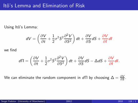
Ito’s Lemma and Elimination of Risk
Using Ito’s Lemma:
dV =
(
∂V
∂t+
1
2σ2S2 ∂2V
∂S2
)
dt +∂V
∂SdS +
∂V
∂IdI
we find
dΠ =
(
∂V
∂t+
1
2σ2S2 ∂2V
∂S2
)
dt +∂V
∂SdS − ∆dS +
∂V
∂IdI .
We can eliminate the random component in dΠ by choosing ∆ = ∂V∂S
.
Sergei Fedotov (University of Manchester) 20912 2010 118 / 1

Modified Black-Scholes Equation
By using No-Arbitrage Principle, and the equation
dI = Sdt
we can obtain the modified Black-Scholes PDE for the Asian option price:
∂V
∂t+
1
2σ2S2 ∂2V
∂S2+ rS
∂V
∂S− rV + S
∂V
∂I= 0.
The value of Asian option must be calculated numerically (no analyticalsolution!)
Sergei Fedotov (University of Manchester) 20912 2010 119 / 1