
Lectures on Statistical Physics - s ustaff.math.su.se/mleites/books/berezin-2009-lectures.pdf ·...
190
Felix Berezin Lectures on Statistical Physics Translated from the Russian and edited by D. Leites Abdus Salam School of Mathematical Sciences Lahore, Pakistan
-
Upload
trankhuong -
Category
Documents
-
view
220 -
download
3
Transcript of Lectures on Statistical Physics - s ustaff.math.su.se/mleites/books/berezin-2009-lectures.pdf ·...

Felix Berezin
Lectures on Statistical Physics
Translated from the Russian and edited by D. Leites
Abdus Salam Schoolof Mathematical SciencesLahore, Pakistan

Summary. The book is an edited and updated transcript of the lectures on Sta-tistical Physics by the founder of supersymmetry theory — Felix Berezin.
The lectures read at the Department of Mechanics and Mathematics of MoscowState University in 1966–67 contain inimitable Berezin’s uniform approach to theBose and Fermi particles, and his unique approach to quantization. These approacheswere used with incredible success in the study of solid state physics, disorder andchaos (K. Efetov), and in a recent (and not yet generally accepted claim of) solutionof one of Clay’s Millennium problems (A. Dynin).
The book is addressed to mathematicians (from sophomore level up) and physi-cists of any level.
ISBN 978-969-9236-02-0c© Dimitry Leites, translation into English and editing, 2009.c© Felix Berezin; his heirs, 2009.

Contents
Author’s Preface . . . . . . . . . . . . . . . . . . . . . . . . . . . . . . . . . . . . . . . . . . . . . vEditor’s preface . . . . . . . . . . . . . . . . . . . . . . . . . . . . . . . . . . . . . . . . . . . . . . vi
Part I The Classical Statistical Physics
1 Background from Classical Mechanics . . . . . . . . . . . . . . . . . . . . . . 3
1 The Ensemble of Microscopic Subsystems . . . . . . . . . . . . . . . . . 92 Physical assumptions. Ergodic Hypothesis. Gibbs’s distribution. 93 An heuristic deduction of the Gibbs distribution . . . . . . . . . . . . . 144 A complete deduction of the Gibbs distribution . . . . . . . . . . . . . 175 Relation to thermodynamics . . . . . . . . . . . . . . . . . . . . . . . . . . . . . . 246 Properties of the entropy . . . . . . . . . . . . . . . . . . . . . . . . . . . . . . . . . 337 Analytical appendix to Chapter 1 . . . . . . . . . . . . . . . . . . . . . . . . . 39
2 Real gases . . . . . . . . . . . . . . . . . . . . . . . . . . . . . . . . . . . . . . . . . . . . . . . . . 438 Physical assumptions . . . . . . . . . . . . . . . . . . . . . . . . . . . . . . . . . . . . 439 The Gibbs Distribution in the Small Canonical Ensemble . . . . . 4610 The correlation functions in the small ensemble . . . . . . . . . . . . . 5011 The Bogolyubov equations . . . . . . . . . . . . . . . . . . . . . . . . . . . . . . . . 5512 The Gibbs distribution in the grand ensemble . . . . . . . . . . . . . . . 5913 The Kirkwood–Salzburg equations . . . . . . . . . . . . . . . . . . . . . . . . . 6414 A Relation between correlation functions . . . . . . . . . . . . . . . . . . . 7115 The existence of potential in the grand ensemble . . . . . . . . . . . . 7316 Existence of the potential in the grand ensemble (cont.) . . . . . . 7517 Properties of the grand and small statistical sums . . . . . . . . . . . 8018 The existence of the thermodynamic potential . . . . . . . . . . . . . . . 8419 The mean over the distribution of the number of particles . . . . 8620 Estimates of the small statistical sum . . . . . . . . . . . . . . . . . . . . . . 89

iv Contents
Part II THE QUANTUM STATISTICAL PHYSICS
21 Background from Quantum Mechanics . . . . . . . . . . . . . . . . . . . . . 95
3 Ensemble of microscopic subsystems . . . . . . . . . . . . . . . . . . . . . . . 10322 The mean with respect to time. The ergodic hypothesis. . . . . . . 10323 The Gibbs distribution . . . . . . . . . . . . . . . . . . . . . . . . . . . . . . . . . . . 10624 A relation to thermodynamics. Entropy . . . . . . . . . . . . . . . . . . . . 110
4 Quantum gases . . . . . . . . . . . . . . . . . . . . . . . . . . . . . . . . . . . . . . . . . . . . 11725 The Method of second quantization . . . . . . . . . . . . . . . . . . . . . . . . 11726 Macroscopic subsystems . . . . . . . . . . . . . . . . . . . . . . . . . . . . . . . . . . 12527 The ideal Bose gas . . . . . . . . . . . . . . . . . . . . . . . . . . . . . . . . . . . . . . . 13128 The ideal Fermi gas . . . . . . . . . . . . . . . . . . . . . . . . . . . . . . . . . . . . . . 13629 The BCS model of superconductivity . . . . . . . . . . . . . . . . . . . . . . 14030 A relation between the quantum and classical statistical physics150
Appendix . . . . . . . . . . . . . . . . . . . . . . . . . . . . . . . . . . . . . . . . . . . . . . . . . . . . . . 156A Semi-invariants in the classical statistical physics . . . . . . . . . . . . 157B Continual integrals and the Green function . . . . . . . . . . . . . . . . . 161C Review of rigorous results (R. A. Milnos) . . . . . . . . . . . . . . . . . . . 172
References . . . . . . . . . . . . . . . . . . . . . . . . . . . . . . . . . . . . . . . . . . . . . . . . . . . . . 175
Index . . . . . . . . . . . . . . . . . . . . . . . . . . . . . . . . . . . . . . . . . . . . . . . . . . . . . . . . . . 181

Author’s Preface
I read this lecture course in 1966–67 at the Department of Mechanics andMathematics of the Moscow State University. Currently, statistical physics ismore than 90% heuristic science. This means that the facts established in thisscience are not proved, as a rule, in the mathematical meaning of this wordalthough the arguments leading to them are quite convincing.
A few rigorous results we have at the moment usually justify heuristicarguments. There is no doubt that this situation will continue until rigorousmathematical methods will embrace the only branch of statistical physicsphysicists did not represent with sufficient clarity, namely, the theory of phasetransitions.
I think that at the moment statistical physics has not yet found an ade-quate mathematical description. I believe, therefore, that the classical heuris-tic arguments developed, starting with Maxwell and Gibbs, did not lose theirvalue. The rigorous results obtained nowadays are only worthy, I think, onlyif they can compete in the simplicity and naturalness with the heuristic ar-guments they are called to replace. The classical statistical physics has suchresults: First of all, these are theorems due to Van Hove, and Lee and Yangon the existence of thermodynamic potential and the Bogolyubov–Khatset–Ruelle theorem on existence of correlation functions. The quantum statisticalphysics has no similar results yet.
The above described point of view was the cornerstone of this course. Itried to present the material based on the classical heuristic arguments pay-ing particular attention to the logical sequence. The rigorous results are onlygiven where they are obtained by sufficiently natural methods. Everywherethe rigorous theorems are given under assumptions that maximally simplifythe proofs. The course is by no means an exhaustive textbook on statisticalphysics. I hope, however, that it will be useful to help the reader to compre-hend the journal and monographic literature.
The initial transcription of the lectures was performed by V. Roitburd towhom I am sincerely thankful. Thanks are also due to R. Minlos, who wroteat my request Appendix C with a review of rigorous results.
F. Berezin, 1972

Editor’s preface
It was for a long time that I wanted to see these lectures published: Theyare more lucid than other book on the same topic not only to me but toprofessional physicists, the ones who understand the importance of supersym-metries and use it in their everyday work, as well, see [KM]; they are alsomuch shorter than any other text-book on the topic. The recent lectures byMinlos [M1] is the only exception and, what is unexpected and nice for thereader, these two books practically do not intersect and both are up to date.
In a recent book by V. V. Kozlov1) [Koz], where in a lively and user-friendlyway there are discussed the ideas of Gibbs and Poincare not much understood(or not understood at all) during the past 100 years since they had beenpublished, these notes of Berezin’s lectures are given their due. In particular,Kozlov gives a reference (reproduced below) to an answer to one of Berezin’squestions obtained 30 years after it was posed.
About the same time that F. A. Berezin read this lecture course, he wasclose with Ya.G. Sinai; they even wrote a joint paper [BS]. As one can discerneven from the above preface of usually very outwardly reserved and discreetauthor, Berezin depreciatingly looked at the mathematicians’ activity aimedat construction of rigorous statistical physics. He always insisted on provingtheorems that might have direct applications to physics.
This attitude of Berezin to the general desire to move from problems ofacute interest to physics towards abstract purely mathematical ones of doubt-ful (at least, in Berezin’s view) physical value (we witness a similar trend of“searching the lost keys under the lamp-post, rather than where they were lost,because it it brighter there”in mathematical approaches to economics), theattitude that he did not hide behind politically correct words, was, perhaps,the reason of certain coldness of Berezin’s colleagues towards these lectures.To my astonishment, publication of this book in Russian was not universallyapproved.
One of the experts in the field wrote to me that this was unrealistic thenand still is. The mathematical part of science took the road indicated byDobrushin and Griffiths who introduced the key notion—the limit Gibbs dis-tribution—and then studying the phase transitions based on this notion, see[DLS]. It seems to this expert that this activity came past Berezin, althoughstill during his lifetime (see [DRL, PS]).
Berezin found an elegant approach to the deducing Onsager’s expressionfor the 2D Ising model. He spent a lot of time and effort trying to generalizethis approach to other models but without any (known) success. The 3D caseremained unattainable, cf. [DP], where presentation is based on Berezin’sideas.1 A remarkable mathematician, currently the director of Steklov Mathematical in-
stitute of the Russian Academy of Sciences, Moscow.

Editor’s preface vii
Some experts told me that the content of the lectures was rather standardand some remarks were not quite correct; Minlos’s appendix is outdated andfar too short. Sure. It remains here to make comparison with Minlos’s vividlectures [M1] more graphic.
Concerning the standard nature of material, I’d like to draw attentionof the reader to Berezin’s inimitable uniform approach to the description ofBose and Fermi particles and its quantization, later developed in [B4, B5, B6].Berezin’s quantization is so un-like any of the mathematicians’s descriptionsof this physical term that for a decade remained unclaimed; but is in great de-mand nowadays on occasion of various applications. This part of the book—of considerable volume — is not covered (according to Math Reviews) in anyof the textbooks on Statistical Physics published during the 40 years that hadpassed since these lectures were delivered. Close ideas were recently used withhuge success in the study of the solid body [Ef]. Possible delusions of Berezin,if any are indeed contained in this book, are very instructive to study. As anillustration, see [Dy].
Finally, if these lectures were indeed “of only historical interest”, then thepirate edition (not listed in the Bibliography) which reproduced the preprint(with new typos inserted) would had hardly appear (pirates are neither Sal-vation Army nor idiots, usually) and, having appeared, would not have im-mediately sell out.
On notation. Although some of Berezin’s notation is not conventionalnow (e.g., the English tr for trace pushed out the German sp for Spur) I alwayskept in mind, while editing, an anecdote on a discussion of F. M. Dostoevskywith his editor:
“Fedor Mikhailovich! You wrote here: ‘In the room stood a round table ofoval form’. This is not quite. . . You know. . . ”
Dostoevsky mused and retorted:“Yes, you are right. However, leave as it is.”
Therefore, although in modern texts the notation fn denotes, or shoulddenote, the set consisting of only one element— fn —and not of all vectors fn
for all possible n, whereas in Berezin’s lectures it is just the other way round,I did not edit this: The geniuses have right to insist on their own style. Fewsimilar shortcomings of the lecture style that still remain in this transcript,should not, I think, deter the reader, same as little-o and big-O notation.
In the preprint [B1], bibliographical references were virtually absent. Inthe book [B1], I added the necessary (in my opinion) minimum, in particular,with the latest works (mainly books). I also cited a report from Math. Reviewsclearly illustrating that a number of open problems tackled in this book is stillleft to the reader. In this English version I have corrected several of the typosstill left in the Russian version of the book [B1].
D. Leites, 2006–2009

Part I
The Classical Statistical Physics


1. Background from Classical Mechanics
1.1. Properties of trajectories of mechanical systems. We will only considerso-called conservative systems, i.e., the ones whose energy does not depend on time.Each state of a mechanical dynamical system with n degrees of freedom is describedby a point of a 2n-dimensional phase space. The customary notation of the coor-dinates of the phase space are usually p = (p1, . . . , pn) (generalized momenta) andq = (q1, . . . , qn) (generalized positions). To each physical quantity (more precisely,to each time-independent physical quantity) there corresponds a function f(p, q) inthe phase space. In what follows, speaking about a physical quantity we always havein mind the corresponding function.
The energy whose function is usually denoted by H(p, q) plays a particular role.The function H(p, q) is called the Hamiltonian function or Hamiltonian. The evolu-tion of the system with time is given by the system of differential equations
dpi
dt= −∂H
∂qi,
dqi
dt=
∂H
∂pi. (1.1)
Hereafter we assume that the existence and uniqueness theorem for any initial con-ditions and any t holds for the system (1.1). The following properties of system (1.1)will be needed in what follows:
1) Let p(t, p0, q0), q(t, p0, q0) be a solution of the system (1.1) with the initialconditions
p(0, p0, q0) = p0, q(0, p0, q0) = q0. (1.2)
Let further f(p, q) be a function constant along the trajectories of the system, i.e.,
f(p(t, p0, q0), q(t, p0, q0)) = f(p0, q0). (1.3)
Physical quantities possessing this property are called conserved ones or integrals ofmotion.
If f is differentiable, then differentiating equality (1.3) with respect to t andtaking (1.1) into account we deduce that f satisfies the partial differential equationX
i
∂f
∂pi
∂H
∂qi− ∂f
∂qi
∂H
∂pi
= 0. (1.4)
The expression in the left-hand side of this equation is called the Poisson bracketand denoted by1) [f, H]. The functions satisfying condition (1.4), i.e., such that[f, H] = 0, are said to be commuting with H. It is easy to verify that condition (1.4)is not only necessary but also sufficient for the differentiable function f to be anintegral of motion.
Obviously, if f is an integral of motion, then the trajectory of a system possessingat least one common point with the surface f(p, q) = const entirely belongs to
1 And often by f, H.

4 § 1. Background from Classical Mechanics
this surface. Each conservative dynamical system possesses at least one integral ofmotion. The energy H(p, q) is such an integral. For the proof, it suffices to verify, dueto the above, that the Poisson bracket [H, H] vanishes which is clear. Therefore eachtrajectory of the system lies on a certain surface of constant energy H(p, q) = E.These surfaces play a most important role in statistical physics.
2) Solutions of the system (1.1) form a one-parametric family of self-maps of thephase space:
(p0, q0) 7→ (p(t, p0, q0), q(t, p0, q0)). (1.5)
The existence and uniqueness theorem implies that the map (1.5) is one-to-one
at every t. Since H does not depend on t, and therefore so do the functions∂H
∂q
and∂H
∂pin the right-hand side of (1.1), it follows that the maps (1.5) constitute a
one-parameter group:
p(t, p(τ, p0, q0), q(τ, p0, q0)) = p(t + τ, p0, q0),
q(t, p(τ, p0, q0), q(τ, p0, q0)) = q(t + τ, p0, q0).
3) The Jacobian of the map (1.5) is equal to 1:
D(p(t, p0, q0), q(t, p0, q0))
D(p0, q0)= 1. (1.6)
This equality means that the maps (1.5) preserve the volume element
dp dq = dp0 dq0,
where
dp dq =
nYi=1
dpi dqi and dp0 dq0 =
nYi=1
dp0i dq0
i .
The condition (1.6) is equivalent to the fact that, for any integrable function f(p, q),we have Z
f(p(t, p0, q0), q(t, p0, q0)) dp0 dq0 =
Zf(p, q) dp dq.
Properties 2) and 3) follow from the general theorems of the theory of differentialequations. Let us recall these theorems. For a system of equations
dxi
dt= fi(x1, . . . , xn),
where the fi do not depend on t, we have1) The solutions xi = xi(t, x
01, . . . , x
0n) such that xi(0, x0
1, . . . , x0n) = x0
i form aone-parameter transformation group of the n-dimensional space
x0i 7→ xi(t, x
01, . . . , x
0n). (1.7)
2) The Jacobian of the map (1.7) is equal to (Liouville’s theorem): ∂xi
∂x0j
= e
tR0
P ∂fi∂xi
dt
.
For the Hamiltonian systems, the maps (1.5) preserve the volume becauseX ∂fi
∂xi=X ∂2H
∂pi∂qi− ∂2H
∂pi∂qi
= 0.

§ 1. Background from Classical Mechanics 5
1.2. An invariant measure on the surfaces of constant energy. Denote bySE the surface of constant energy H(p, q) = E, let ξ be a point on SE and ξ(t, ξ0)a trajectory through ξ0.
A measure dξ on SE is said to be invariant if, for any integrable function f(ξ)and any t, the function f(ξ(t, ξ0)) is integrable with respect to ξ0 andZ
f(ξ(t, ξ0)) dξ0 =
Zf(ξ) dξ. (1.8)
An equivalent definition: A measure is said to be invariant if, for any measurable setA and any t, the set At obtained from A under the action of the dynamical system1.7 through time t, and measures of A and At are equal.
To see that the second definition follows from the first one, take for f(ξ) thecharacteristic function of A. The first definition directly follows from the second oneby the definition of Lebesgue’s integral.
Suppose that the surface of constant energy SE is a manifold. Then it can becovered by a system of neighborhoods Uα, each of which is homeomorphic to a ballin a (2n − 1)-dimensional Euclidean space. Let ξ1, . . . , ξ2n−1 be local coordinatesin Uα. If the measure in each Uα is of the form
dξ = ω(ξ) dξ1 . . . dξ2n−1,
where ω(ξ) is a Lebesgue-integrable in Uα function, then the measure dξ in SE will bereferred to absolutely continuous with respect to Lebesgue measure. If the measure inSE is absolutely continuous with respect to Lebesgue measure, then it is invariantif (1.8) holds only for continuous functions with compact support. Moreover, itsuffices to consider functions that are non-zero only within a coordinate patch. Thisfollows from the fact that if the measure is absolutely continuous with respect toLebesgue measure, then such functions are dense in L1(SE). The following is themain theorem of this section.
1.3. Theorem. If the Hamiltonian function H(p, q) is continuously differentiable,then the non-singular surface of constant energy is a manifold and it possesses aninvariant measure absolutely continuous with respect to Lebesgue measure.
Recall that the surface H(p, q) = E is said to be non-singular, if∂H
∂piand
∂H
∂qi
do not vanish anywhere on the surface for all i.The fact that under these conditions the surface SE is a manifold follows from
the implicit function theorem. Each point ξ ∈ SE possesses a neighborhood Uξ
in which the equation H(p, q) = E is solvable for one of the coordinates. Let, fordefiniteness’ sake, this coordinate be p1. Then, in Uξ, the equation of SE takes theform
p1 = f(p2, . . . , pn, q1, . . . , qn),
where p2, . . . , pn, q1, . . . , qn are local coordinates in Uξ. Let f(p, q) be a continuousfunction, ϕ(ξ) its value on SE . Consider the integral
Ih =1
h
ZE≤H(p,q)≤E+h
f(p, q) dp dq, (1.9)
over the part of the phase space confined between SE and SE+h. Let us show thatthe limit lim
h−→0Ih exists. For this, in the phase space, in a neighborhood of SE ,
6 § 1. Background from Classical Mechanics
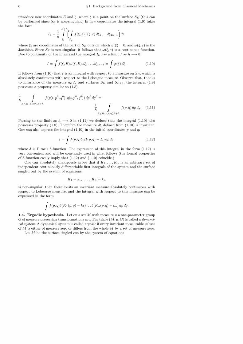
introduce new coordinates E and ξ, where ξ is a point on the surface SE (this canbe performed since SE is non-singular.) In new coordinates the integral (1.9) takesthe form
Ih =1
h
E+hZE
ZSE
f(ξ, ε)ω(ξ, ε) dξ1 . . . dξ2n−1
dε,
where ξi are coordinates of the part of SE outside which ϕ(ξ) = 0, and ω(ξ, ε) is theJacobian. Since SE is non-singular, it follows that ω(ξ, ε) is a continuous function.Due to continuity of the integrand the integral Ih has a limit I as h −→ 0:
I =
Zf(ξ, E)ω(ξ, E) dξ1 . . . dξ2n−1 =
Zϕ(ξ) dξ. (1.10)
It follows from (1.10) that I is an integral with respect to a measure on SE , which isabsolutely continuous with respect to the Lebesgue measure. Observe that, thanksto invariance of the measure dp dq and surfaces SE and SE+h, the integral (1.9)possesses a property similar to (1.8):
1
h
ZE≤H(p,q)≤E+h
f(p(t, p0, q0), q(t, p0, q0)) dp0 dq0 =
1
h
ZE≤H(p,q)≤E+h
f(p, q) dp dq. (1.11)
Passing to the limit as h −→ 0 in (1.11) we deduce that the integral (1.10) alsopossesses property (1.8). Therefore the measure dξ defined from (1.10) is invariant.One can also express the integral (1.10) in the initial coordinates p and q:
I =
Zf(p, q)δ(H(p, q)− E) dp dq, (1.12)
where δ is Dirac’s δ-function. The expression of this integral in the form (1.12) isvery convenient and will be constantly used in what follows (the formal propertiesof δ-function easily imply that (1.12) and (1.10) coincide.)
One can absolutely analogously prove that if K1, . . . , Kα is an arbitrary set ofindependent continuously differentiable first integrals of the system and the surfacesingled out by the system of equations
K1 = k1, . . . , Kα = kα
is non-singular, then there exists an invariant measure absolutely continuous withrespect to Lebesgue measure, and the integral with respect to this measure can beexpressed in the formZ
f(p, q)δ(K1(p, q)− k1) . . . δ(Kα(p, q)− kα) dp dq.
1.4. Ergodic hypothesis. Let on a set M with measure µ a one-parameter groupG of measure preserving transformations act. The triple (M, µ, G) is called a dynami-cal system. A dynamical system is called ergodic if every invariant measurable subsetof M is either of measure zero or differs from the whole M by a set of measure zero.
Let M be the surface singled out by the system of equations

§ 1. Background from Classical Mechanics 7
K1 = k1, . . . , Kα = kα,
where the Ki(p, q) are the first integrals of the mechanical system. By the above, ifM is non-singular, then it possesses an invariant measure, and therefore a dynamicalsystem arises.
1.4.1. Question. Is it ergodic?
To answer this question is extremely important in order to justify equilibriumstatistical physics. The assumption on ergodicity of M is called the ergodic hy-pothesis. Obviously, the most important is the case where M = SE is the surface ofconstant energy. We will discuss relations of the ergodic hypothesis with justificationof statistical physics in the next section.
1.5. A relation of the mean with respect to time and the mean overthe surface of constant energy (microcanonical mean). First of all, letus formulate the physical hypothesis concerning the properties of the devices thatinvestigate the systems consisting of microscopic subsystems.
Our devices do not measure the instant values of physical quantities but rathertheir mean values
1
T
TZ0
f(q(t, p0, q0), p(t, p0, q0)) dt, (1.13)
whereq(t, p0, q0), p(t, p0, q0)
is the trajectory of the system passing through the
point (p0, q0) at t = 0. The time T of relaxation of the devices is essentially greaterthan the lifespan of the processes, so the mean (1.13) can be replaced by the limit
limT−→∞
1
T
TZ0
f(p(t, p0, q0), q(t, p0, q0)) dt, (1.14)
which is called the mean of f with respect to time.A mathematical discussion is possible starting from here.Suppose that a dynamical system that appears on the surface of constant energy
SE is ergodic and for any E the surface SE possesses a finite measure. In this case thevon Neumann’s ergodic theorem implies that the mean with respect to time (1.14) isequal to the mean over the surface SE on which this trajectory lies. Let us formulatevon Neumann’s theorem:
1.5.1. Theorem. Let there be given an ergodic dynamical system on a set Mwith finite measure µ(M) < ∞ and let x(y, t) be a trajectory of this system passingthrough a point y. Then, for any function f ∈ L2(M, µ), there exists a limit (with
respect to L2(M, µ))-convergence) of functions fT (y) =1
T
TR0
f(x(y, t)) dt, equal to
limT−→∞
1
T
TZ0
f(x(y, t)) dt =1
µ(M)
ZM
f(x) dµ(x).
The limit does not depend on the initial point y.

8 § 1. Background from Classical Mechanics
Recall that, by a hypothesis above, we haveZδ(H(p, q)− E) dp dq < ∞.
Therefore, under our conditions, this theorem implies that, for a given ergodic sys-tem, we have
limT−→∞
1
T
TZ0
f(p(t, p0, q0), q(t, p0, q0)) dt =
Rf(p, q)δ(H(p, q)− E) dp dqR
δ(H(p, q)− E) dp dq. (1.15)
The right-hand side of (1.15) is the mean of f on the surface of constant energy.According to the accepted physical terminology this mean is called the microcanon-ical one.

Chapter 1
The Ensemble of Microscopic Subsystems
This chapter is devoted to the study of mechanical systems consisting of ahuge number N of weakly interacting identical microscopic subsystems. Un-like the whole system, each subsystem is described by few parameters. Wesuppose that no subsystem interacts with any objects outside the system. Mi-croscopic nature of an individual subsystem means that it does not depend onthe total number N of subsystems in the ensemble. The study of ensembles ofmicroscopic subsystems is mainly of methodological value. The most popularin statistical physics ensembles (real gases) consist of macroscopic subsystems.For an example of ensemble of microscopic subsystems (with certain reserva-tions discussed in § 5)), we can take an ideal gas confined in a macroscopicvessel, e.g., in a closed thermos. For an individual microscopic subsystem wecan take a molecule of the gas. The number of subsystems1) is of the order ofmagnitude of the Avogadro number ∼ 1027.
2. Physical assumptions. Further discussion of ErgodicHypothesis. Gibbs’s distribution
2.1. The microcanonical mean. We will use the following notation: Wedenote the total set of all phase variables of the system by (P, Q), whereasthe set of phase variables describing the α-th subsystem will be denoted by(p(α), q(α)). Therefore,
(p(α), q(α)) =(p(α)
i , q(α)i )
, where i = 1, . . . , n.
1 Let us give one more definition of the microscopic subsystem which apparentlybetter describes the physical nature of the situation. The subsystem is said tobe microscopic if the number of its degrees of freedom does not depend on thetotal number of subsystems in the ensemble. Under such a definition the idealgas becomes the ensemble of microscopic subsystems without any reservations.
I did not use this definition since I do not know how to generalize it to thequantum case. I thought that different definitions of microscopic subsystem forthe classical and quantum cases would violate the uniformity of my narrative.

10 Ch. 1. The Ensemble of Microscopic Subsystems
In this notation, (P,Q) =(p(α)
i , q(α)i )
, where α = 1, . . . , N , i = 1, . . . , n. Let
dP dQ denote the volume element in the phase space of the system
dP dQ =∏
i,α
dp(α)i dq
(α)i .
In this notation, the Hamiltonian of the system takes the form
Hε(P, Q) =N∑
α=1
H(p(α), q(α)) + vε(P, Q), (2.1)
where H(p(α), q(α)) is the Hamiltonian of an individual subsystem and vε(P,Q)is the interaction energy of subsystems which is supposed to be very small.The parameter ε is introduced for our convenience in such a way thatlim
ε−→0vε(P, Q) = 0. Let
H =N∑
α=1
H(p(α), q(α)) (2.2)
denote the Hamiltonian obtained from Hε as ε −→ 0. The function H isthe Hamiltonian of the system consisting of non-interacting subsystems. Thissystem is not ergodic1).
We will make the following two assumptions:1) There exists a limit of means with respect to time as ε −→ 0
limε−→0
limT−→∞
1
T
T∫
0
f(Pε(t),Qε(t)) dt, (2.3)
where Pε(t) and Qε(t) are trajectories of the system with Hamiltonian Hε
(our assumption that the interaction between the subsystems is“small” means
that the mean limT−→∞
1
T
T∫0
f(Pε(t), Qε(t)) dt is, with high accuracy, equal to the
limit (2.3).2) The system is ergodic for ε 6= 0. Therefore
limT−→∞
1
T
T∫
0
f(Pε(t), Qε(t)) dt =R
f(P, Q)δ(H − E) dP dQRδ(H − E) dP dQ
. (2.4)
1 Obviously, for the system with Hamiltonian (2.2), the functionsHα = H(p(α), q(α)) are integrals of motion. The surface of constant energySE is fibrated into invariant sets singled out by the equations H(p(α), q(α)) = hα
(α = 1, . . . , N). Therefore SE possesses invariant subsets of non-zero andnon-full measure. For example, the subset of points (P, Q) ∈ SE , such thata < H(p(1), q(1)) < b for an appropriate choice of a and b.

§ 2. Physical assumptions. Ergodic Hypothesis. Gibbs’s distribution. 11
The right-hand side of (2.4) is continuous with respect to ε at ε = 0, andtherefore
limε−→0
limT−→∞
1
T
T∫
0
f(Pε(t), Qε(t)) dt =R
f(P, Q)δ(H − E) dP dQRδ(H − E) dP dQ
, (2.5)
where H is the Hamiltonian of the (non-ergodic!) system consisting of non-interacting subsystems.
Thus the mean with respect to time of f is replaced by its microcanonicalmean (2.5) with Hamiltonian function H that generate highly non-ergodicsystem.
2.2. Gibbs’s distribution. Highly interesting for statistical physics are themean values of quantities that behave similarly to energy. (Such quantities aresometimes called summatory):
F(N)(P,Q) = 1
N
∑f(p(α), q(α)). (2.6)
Let ε = E
Nbe the mean energy of the subsystem. In what follows, we pass
to the limit as N −→ ∞. It is essential that ε does not depend on N . Themicrocanonical mean of F(P,Q) is equal to
F(N)
E =R
F(P, Q)δ(H(P, Q)−Nε) dP dQRδ(H(P, Q)−Nε) dP dQ
.
Taking into account the form of F(N)E , we see that
F(N)
E =∫
f(p, q)ρN (p, q) dp dq, (2.7)
where
ρN (p, q) =
Rδ
N−1Pα=1
H(p(α), q(α)) + H(p, q)−Nε
N−1Qα=1
dp(α) dq(α)Rδ
N−1Pα=1
H(p(α), q(α))−Nε
N−1Qα=1
dp(α) dq(α)
. (2.8)
It turns out there exists a limit ρ(p, q) = limN−→∞
ρN (p, q). Since N is very big,
it follows that the mean (2.7) coincides, with good accuracy, with its limit asN −→∞ which is equal to1)
Fmicrocan. = fGibbs =∫
f(p, q)ρ(p, q) dp dq.
The function ρ(p, q) is the density of the probability distribution called Gibbs’sdistribution or the canonical distribution. We will compute this function inwhat follows. It turns out to be equal to1 In § 4, we will estimate the rate of convergence of
RfρN dp dq to its limit.

12 Ch. 1. The Ensemble of Microscopic Subsystems
ρ(p, q) = e−βH(p,q)Re−βH(p,q) dp dq
,
where the parameter β is determined from the equation
ε =R
He−βH dp dqRe−βH dp dq
.
The described above passage to the limit as N −→ ∞ is oftencalled“thermodynamic”, and various quantities obtained under passage to thislimit are called“thermodynamic limits”. In case where the subsystem possessesapart from energy the first integrals K1, . . . , Ks and the interaction v′ε is suchthat the quantities
Ki = Ki(p1, q1) + Ki(p2, q2) + . . .
are preserved and on the surfaces Ki = Nki the ergodic dynamical systemsappear, the microcanonical mean (2.5) is replaced by
F(N)
E,K2,...,KS=R
Fδ(H −Nε)δ(K1 −Nk1) . . . δ(Ks −Nks) dP dQRδ(H −Nε)δ(K1 −Nk1) . . . δ(Ks −Nks) dP dQ
.
The corresponding density of the Gibbs’s distribution is equal to
ρ(p, q) = e−β(H(p,q)+µ1K1(p,q)+...+µSKS(p,q))Re−β(H(p,q)+µ1K1(p,q)+...+µSKS(p,q)) dp dq
,
where the parameters β and µi are determined from the equations∫
H(p, q)ρ dp dq = ε,
∫Kiρ dp dq = ki.
2.3. Discussion of hypotheses. First of all, we note that the system underthe study is very close to a non-ergodic one and it is precisely this definitelynon-ergodic system consisting of non-interacting subsystems that plays themain role for us. The nature of interactions between subsystems is irrelevant,only the fact that it is“small” is important. Therefore theorems on ergodicityof a certain concrete dynamical system are immaterial1).
To justify the passage from the mean with respect to time to the meanover the surface of constant energy ,the following type of theorem is sufficient:
2.3.1. Hypothesis (Conjecture). Consider dynamical systems with Hamil-tonian functions of the form H = H0+V , where H0 is a fixed function and V isa variable function running over a topological space. For an everywhere denseset of functions V , the dynamical systems with Hamiltonian H = H0 + V areergodic.1 In what follows, we will see that the systems consisting of macroscopic subsystems
is a totally different matter.

§ 2. Physical assumptions. Ergodic Hypothesis. Gibbs’s distribution. 13
Even a more rough question is of interest.
2.3.2. Question. Is it true that, in a natural topology in the space of dy-namical systems, the ergodic systems constitute a dense set?
Returning to the above formulated hypothesis, let us give an example ofHamiltonian functions interesting from this point of view:
H = H0 + εV (q), where ε > 0,
H0 = (q01 + ωp2
1) + . . . + (q2n + ωp2
n),(2.9)
and V (q) ≥ 0 is a 4-th degree polynomial in totality of the variables q1, . . . , qn.The coefficients of non-negative 4-th degree polynomials constitute a set D inthe finite-dimensional space of the coefficients of all 4-th degree polynomialsin n variables.
2.3.3. Question. Is it true that, for all points of D, except a set of Lebesguemeasure zero (or perhaps the set consisting of the union of manifolds of smallerdimension), the systems are ergodic? 1)
2.3.4. Hypothesis. In the microcanonical mean (2.4) one can pass to thelimit as ε −→ 0, and the microcanonical mean (2.5) is the limit.
This hypothesis is a precise mathematical equivalent of the physical as-sumption that the interactions are “small”. The hypothesis can be justifiedfor appropriate potentials with the help of usual theorems on passage to thelimit under the integral sign. For example, for Hamiltonian functions of theform (2.9), such a passage is definitely possible.
The above described point of view on the relation between the mean withrespect to time and over the surface of constant energy is traditional thoughit is very seldom expressed with sufficient clarity.
In this relation a principal question arises: Assume that our system canbe approximated by ergodic systems. Consider the mean with respect to time
ϕ(p, q, T ) = 1
T
T∫
0
F (p(t), q(t)) dt,
where (p(t), q(t)) is the trajectory of the system corresponding to the param-eter ε. Will the rate with which ϕ tends to the limit as T −→∞ decay fast asε −→ 0? If this were so for the systems with Hamiltonians of the form (2.1)and function F of the form (2.6) then the above arguments would lose a gooddeal of their physical meaning.
1 For the answer obtained 30 years after Berezin posed the question, see [U]; for aninterpretation, see [Koz]. — Ed.

14 Ch. 1. The Ensemble of Microscopic Subsystems
3. An heuristic deduction of the Gibbs distribution
3.1. A combinatorial problem. Our nearest goal is the proof of existenceof the limit ρ(p, q) = lim
N−→∞ρN (p, q) and the equality
ρ(p, q) = e−βH(p,q)Re−βH(p,q) dp dq
, (3.1)
where ρN is given by formula (2.8).In this section, we use simple graphic arguments; in the next one we give
a rigorous proof.Let us split the phase space of the subsystem into cubic cells with side l.
We will only consider the states of subsystems for which the points depictingthem lie strictly inside a cell. To each such system we assign a state whosepoint coincides with the center of the cell.
In this way, we obtain an auxiliary lattice subsystem. It is intuitively clearthat the auxiliary system consisting of such subsystems turns into the initialone as l −→ 0.
Hereafter and to the end of the section, (p, q) denotes a point of the latticewhose vertices are the centers of the cells.
Let (P,Q) = (p(1), . . . , p(N), q(1), . . . , q(N)) be a state of the total systemand let among the coordinates p(α), q(α) there be N(p, q) equal with eachother and equal to p and q, respectively.
The occupation number N(p, q) is equal to the number of subsystems whosestates are depicted by the points lying inside the cell centered at (p, q). Obvi-ously ∑
N(p, q) = N. (3.2)
Further, if the point (P, Q) lies on the surface SE , then its occupationnumber satisfies, in addition to (3.2), the relation
∑N(p, q)H(p, q) = Nε, (3.3)
obtained from the equation∑
H(p(α), q(α)) = E of the surface SE by simpli-
fication. The parameter ε = E
Ncan be interpreted as the mean energy of the
subsystem.The set N(p, q) of non-negative integers satisfying conditions (3.2)
and (3.3) is said to be admissible.Obviously, each admissible set N(p, q) is the set of occupation numbers
for a certain state (P,Q) ∈ SE .The mean of a function F over the surface SE is equal to
FE =
P(P,Q)∈SE
F(P, Q)PP,Q∈SE
1. (3.4)

§ 3. An heuristic deduction of the Gibbs distribution 15
If F = F(N)(P,Q) = 1
N
∑f(p(α), q(α)), then after simplification we get
F(N)(P, Q) = 1
N
∑p,q
N(p, q)f(p, q), (3.5)
where N(p, q) are the occupation numbers corresponding to the point (P, Q).Obvious combinatorial considerations make it obvious that the number of
distinct states (P, Q) with the same set N(p, q) of occupation numbers is
equal to N !Qp,q
N(p, q)!. Therefore
∑
(P,Q)∈SE
F(N)(P, Q) = 1
N
∑
N(p,q)
N !Qp,q
N(p, q)!
∑N(p, q)f(p, q). (3.6)
The outer sum in the right-hand side of (3.6) runs over all admissible sets ofnon-negative integers. Applying (3.6) to the case where f(p, q) ≡ 1, we find∑P,Q∈SE
1 and
F(N)
E =
PN(p,q)
N !Qp,q
N(p, q)!
P(p,q)
N(p, q)
Nf(p, q)
PN(p,q)
N !Qp,q
N(p, q)!
, (3.7)
where the outer sum in the numerator and the sum in the denominator runsover all admissible sets N(p, q) of non-negative integers.
Our goal is to find the limit of the mean values (3.4) and (3.7).
3.2. A solution of the combinatorial problem. The following trans-formations of equation (3.7) are related with its probabilistic interpretation.Observe that (3.7) is the mathematical expectation of the random quantity
ϕ =∑ N(p, q)
Nf(p, q), (3.8)
in which the admissible set of numbers N(p, q) depends on chance and theprobability of the set N(p, q) is equal to
N !Qp,q
N(p, q)!PN(p,q)
N !Qp,q
N(p, q)!
. (3.9)
Observe although this is inessential in what follows that the quantity ϕ it-self for a fixed set N(p, q) is also the mathematical expectation of the func-tion f(p, q) depending on a random point (p, q) distributed with probabilityN(p, q)
N.

16 Ch. 1. The Ensemble of Microscopic Subsystems
In what follows, we will find the most probable set N(p, q), i.e., suchthat (3.9) attains its maximum and replace the mean of (3.8) over all sets bythe value of ϕ for the most probable set.
Obviously, the expression (3.9) and its numerator attain their maximumfor the same values of N(p, q). Taking logarithm of the numerator of (3.9) andusing the Stirling formula for N(p, q)!, we find N(p, q) from the equations
∂
∂N(p, q)
((ln N !−
∑N(p, q)(lnN(p, q)− 1)
)−
β∑
N(p, q)H(p, q)− µ∑
N(p, q))
= 0, (3.10)
where β and µ are the Lagrange multipliers corresponding to (3.2)) and (3.3).Equation (3.10) has the only solution
N(p, q) = Ce−βH(p,q), where C = eµ. (3.11)
The fact that the expression (3.11) determines the maximum of the functionwe are interested in and not any other extremal is obvious, in a sense, sincethe equation (3.10) has the only solution.
We find the constants C and β from equations (3.2) and (3.3):PH(p, q)e−βH(p,q)P
e−βH(p,q)= ε, C = NP
e−βH(p,q). (3.12)
Having replaced in (3.7) the sum over all admissible sets N(p, q) by the valueof ϕ for the most probable set we find:
FE =∑ e−βH(p,q)P
e−βH(p,q)f(p, q). (3.13)
Multiplying the numerator and denominator in (3.11) and (3.13) by ln (thevolume of the cell) we see that all sums in these formulas are integral ones.Passing to the limit as l −→ 0 we finally obtain
ε =R
H(p, q)e−βH(p,q) dp dqRe−βH(p,q) dp dq
, (3.14)
FE =∫
f(p, q)ρ(p, q) dp dq, (3.15)
where
ρ(p, q) = e−βH(p,q)Re−βH(p,q) dp dq
. (3.16)
The mathematically flawless deduction of the Gibbs distribution based on theconsiderations developed in this section is hardly possible.
The main difficulty is the reduction to the combinatorial problem, i.e., to for-mula (3.7). Contrariwise the solution of combinatorial problem (i.e., the proof of the

§ 4. A complete deduction of the Gibbs distribution 17
relation limN−→∞
F(N)E = FE , where F
(N)E is determined by (3.7) and FE is determined
by (3.15)) can be made quite rigorous under broad assumptions concerning H(p, q)and f(p, q). For this, one can use Laplace transformation in the same way we applyit in the next section.
Therefore, the complete deduction (given shortly) is based on another ideawhich is not so graphic.
4. A complete deduction of the Gibbs distribution
4.1. Formulation of the main theorem. In this section we will prove theexistence of the limit as N −→∞ of the functions ρN (p, q), cf. (2.8):
ρN (p, q) =
Rδ
N−1Pα=1
H(p(α), q(α)) + H(p, q)−Nε
N−1Qα=1
dp(α) dq(α)Rδ
NP
α=1
H(p(α), q(α))−Nε
NQ
α=1
dp(α) dq(α)
. (4.1)
and compute it. In what follows it is convenient to denote the area of thesurface of constant energy of the subsystem by
ω(ε) =∫
δ(H(p, q)− ε) dp dq. (4.2)
4.1.1. Theorem. Let H(p, q) satisfy the conditions1) H(p, q) ≥ 0,2) ω(ε) is monotonically non-decreasing and differentiable,3) ω(ε) ∼ εp, where p > 0 as ε −→ 0,4) ω(ε) ∼ εq, where q > 0 as ε −→ +∞,5) The function e−βεω′(ε) is integrable for any β > 0.
Then1) The sequence ρN (p, q) tends to
ρ(p, q) = e−βH(p,q)Re−βH(p,q)
,
where β = β(ε) > 0 is the only root of the equationRH(p, q)e−βH(p,q) dp dqR
e−βH(p,q) dp dq= ε. (4.3)
2) For any measurable function f(p, q) such that∫|f |e−βH dp dq < ∞,
∫|f |He−βH dp dq < ∞,
the limit exists:lim
N−→∞
∫fρN dp dq =
∫fρ dp dq.

18 Ch. 1. The Ensemble of Microscopic Subsystems
Proof. Denote by aN (p, q | ε) the numerator of (4.1) and ΩN (ε) the denom-inator of (4.1). Let us study the asymptotics of these functions as N −→ ∞.Since ΩN =
∫aN dp dq, it suffices to consider aN . Observe that Ω1(ε) = ω(ε)
is given by (4.2). Further,
δ
( N∑α=1
H(p(α), q(α))− x
)=
∞∫
−∞δ(H(p(N), q(N))− y)δ
(N−1∑α=1
H(p(α), q(α))− (x− y))
dy.
Integrating this equation againstN∏
α=1dp(α) dq(α) and
N−1∏α=1
dp(α) dq(α) and using
the fact that ΩN (ε) = 0 for ε < 0 we deduce:
ΩN
(x
N
)=
∞∫
−∞ω(y)ΩN−1
(x− y
N − 1
)dy =
x∫
0
ω(y)ΩN−1
(x− y
N − 1
)dy,
aN
(ξ, η | x
N
)=
∞∫
−∞δ(H(ξ, η)− y)ΩN−1
(x− y
N − 1
)dy = ΩN−1
(x−H(ξ, η)
N − 1
).
Thus the functions ΩN and aN are expressed in terms of ω by means ofmultiple convolutions. Therefore, to study them, the Laplace transformation1)
is convenient. Using the formulas found and the condition of the theorem wefind by the induction that the function aN (ξ, η | ε) grows as a power of ε forfixed ξ, η. Therefore the Laplace transform of aN (ξ, η | ε) exists. Denote theLaplace transform of aN by AN :
AN (ξ, η | t) =
∞∫
0
aN (ξ, η | ε)e−tε dε =
∞∫
0
∫δ
(N−1∑α=1
H(p(α), q(α)) + H(ξ, η)−Nε
) N−1∏α=1
dp(α) dq(α)e−tε dε =
1
N
∫e−(
N−1Pα=1
H(p(α),q(α))+H(ξ,η)
)tN
N−1∏α=1
dp(α) dq(α) =
1
Ne−
tN
H(ξ,η)
(∫e−
tN
H(p,q) dp dq
)N−1
.
The inverse transform is equal to1 For the necessary background on Laplace transformations, see § 7.

§ 4. A complete deduction of the Gibbs distribution 19
aN (ξ, η | ε) = 1
2π
∞∫
−∞AN (ξ, η | N(λ + iτ))eN(λ+iτ)ε dτ =
1
2π
∞∫
−∞ψ(ξ, η | τ)e(N−1)ϕ(τ) dτ, (4.4)
where
ψ(ξ, η | τ) = e−(λ+iτ)(H(ξ,η)−ε),
ϕ(τ) = ln∫
e−(λ+iτ)(H(ξ,η)−ε) dp dq.(4.5)
It turns out that the functions ψ and ϕ satisfy the following conditions:ψ(ξ, η | τ) is bounded and continuously differentiable with respect to τ ;ϕ is three times continuously differentiable, moreovera) ϕ(0) is real,b) ϕ′(0) = 0,c) ϕ′′(0) is real and ϕ′′(0) = −α < 0,d) for any δ > 0, there exists K = K(δ) > 0 such that
∫
|t|>δ
eNRe (ϕ(t)−ϕ(0)) dt < KN .
We only have to prove, obviously, properties a)–d) of ϕ. We will postpone thisproof to the end of the section where we will also establish that the propertyb) is satisfied for the only value λ = β which is a solution of equation (4.3).
Properties a)–c) coincide with the properties a)–c) of Theorem 7.1 and theproperty d) above guarantees fulfillment of the property d) of Theorem 7.1with the constant σ = 1. Thus, we can apply Theorem 7.1. By this theorem,for a sufficiently large N , we have
aN (ξ, η | ε) = 1
2π
√π
Nα
(ψ(0)
(1 + c(N)√
N
)+ b(N)√
N
), (4.6)
where c(N) and b(N) satisfy
|c(N)| ≤ 2max|t|<δ
∣∣∣ϕ(0)− αt2
αt3
∣∣∣,
|b(N)| ≤ 2 supt|ψ(t)|+ max
|t|<δ
∣∣∣ψ(t)− ψ(0)
t
∣∣∣.
Observe that, in our case, for λ = β, we have
|ψ| = e−β(H(ξ,η)−ε),∣∣∣ψ(t)− ψ(0)
t
∣∣∣ =∣∣∣e−(β+it)(H−ε) − e−β(H−ε)
t
∣∣∣ =
2e−β(H−ε)
∣∣∣∣ sint(H−ε)
2
t
∣∣∣∣ ≤ |H(ξ, η)− ε|e−β(H−ε).

20 Ch. 1. The Ensemble of Microscopic Subsystems
Thus, for a sufficiently large N , the function aN (ξ, η | ε) is representable inthe form
aN (ξ, η | ε) = aN (ξ, η | ε) 1
2π
√π
NαeNϕ(0)+βε,
whereaN (ξ, η | ε) = e−βH(ξ,η)
(1 + c′(N) + H(ξ, η)d(N)√
N
), (4.7)
d(N) and c′(N) are bounded by constants independent of N , ξ, η. Obviously,
ρN (ξ, η) = aN (ξ, η)RaN (ξ, η) dξ dη
.
Unlike aN , the function aN possesses a limit as N −→∞:
limN−→∞
aN (ξ, η | ε) = e−βH(ξ,η). (4.8)
Let a function f(ξ, η) be such that∫|f(ξ, η)|H(ξ, η)e−βH(ξ,η) dξ dη < ∞,
∫|f(ξ, η)|e−βH(ξ,η) dξ dη < ∞.
(4.9)
(Observe that f(ξ, η) ≡ 1 satisfies these conditions.) Consider a sequence offunctions fN = aNf , where each fN is bounded by an integrable function
∣∣∣f(ξ, η)e−βH(ξ,η)(1+ c′(N)+ d(N)H(ξ, η)√
N
)∣∣∣ <∣∣∣f(ξ, η)e−βH(ξ,η)
(1+ c′+ dH(ξ, η)
)∣∣∣,
and where c′ and d are functions that bind c′(N) and d(N) (|c′(N)| ≤ c′ and|d(N)| ≤ d). Let, moreover, the sequence fN (ξ, η) converge to f(ξ, η)e−βH(ξ,η).We can apply Lebesgue’s theorem. Therefore there exists the limit of integrals∫
faN dξ dη equal to
limN−→∞
∫f(ξ, η)aN (ξ, η) dξ dη =
∫f(ξ, η)e−βH(ξ,η) dξ dη.
In particular, for f ≡ 1, we get
limN−→∞
∫aN (ξ, η) dξ dη =
∫e−βH(ξ,η) dξ dη.
Taking (4.8) into account we deduce the existence of the limit of the ρN asN −→∞ and the equality
limN−→∞
ρN (ξ, η) = e−βH(ξ,η)Re−βH(p,q) dp dq
.

§ 4. A complete deduction of the Gibbs distribution 21
Therefore, for the function f satisfying conditions (4.9), we have
limN−→∞
∫ρN (ξ, η)f(ξ, η) dξ dη =
∫f(ξ, η)ρ(ξ, η) dξ dη.
To complete the proof of the theorem, it suffices to verify that ϕ satisfiesconditions a)–d).
It is obvious that ϕ(0) is real. Further,
ϕ′(τ) = −i
R(H(p, q)− ε)e−(λ+iτ)(H(p,q)−ε) dp dqR
e−(λ+iτ)(H(p,q)−ε) dp dq= −i(Hλ+iτ − ε), (4.10)
where
Hλ+iτ =R
H(p, q)e−(λ+iτ)H(p,q) dp dqRe−(λ+iτ)H(p,q) dp dq
.
Let us show that, for τ = 0, we have
d
dλHλ < 0,
Indeed:
dHλ
dλ=
RHe−λH dp dq
2
− R H2e−λH dp dqR
e−λH dp dqRe−λH dp dq
2 .
Now apply the Cauchy inequality:
(∫He−λH dp dq
)2
=(∫
He−12
λHe−12
λH dp dq)2
≤∫
H2e−λH dp dq
∫e−λH dp dq.
The equality can only happen when He−λH2 is proportional to e−
λH2 ; this is
impossible. Therefore, we always have a strict inequality
dHλ
dλ< 0. (4.11)
Hence Hλ strictly monotonically decays.Let us investigate the behavior of Hλ as λ −→ 0 and λ −→∞. We have
Hλ =R
H(p, q)e−λH(p,q) dp dqRe−λH(p,q) dp dq
=
∞R0
εe−λεω(ε) dε
∞R0
e−λεω(ε) dε
.
Recall that from the very beginning we required that H(p, q) should be suchthat the function ω(ε) grows polynomially as ε −→ ∞ and decays polynomi-ally as ε −→ 0.

22 Ch. 1. The Ensemble of Microscopic Subsystems
First, consider the case λ −→∞. We have
∞∫
0
e−λεω(ε) dε =
a∫
0
e−λεω(ε) dε +
∞∫
a
e−λεω(ε) dε. (4.12)
The number a is selected so that |ω(ε) − rεp| < δεp for 0 < ε < a andcertain r and δ. We also have
a∫
0
e−λεω(ε) dε < (r + δ)
a∫
0
εpe−λε dε ≈ r + δ
λp+1Γ (p + 1) as λ −→∞.
Let us estimate the second summand in (4.12):
∞∫
a
e−λεω(ε) dε = e−λε0
∞∫
a
e−λ(ε−ε0)ω(ε) dε < Ce−λε0 , where ε0 < a.
Thus,∞∫
0
e−λεω(ε) dε ≈ C1
λp+1as λ −→∞.
Similar estimates show that∞∫
0
εe−λεω(ε) dε ≈ C2
λp+2as λ −→∞.
HenceHλ −→ 0 as λ −→∞.
It is the integral∞∫a
that gives the main contribution to∞∫0
e−λεω(ε) dε as
λ −→ 0 (and not the integrala∫0
, as is the case as λ −→ ∞). Easy estimates
show that Hλ −→∞ not more slow than C3λ−1 as λ −→ 0.
Thus, Hλ strictly monotonically decays and, moreover, limλ−→0
Hλ = +∞,
limλ−→∞
Hλ = 0. Therefore the equation Hλ − ε = 0 possesses a unique root β.
Thus, we have established that a unique value λ = β possesses property b).Further, due to (4.11) and (4.10) we have
ϕ′′(0) = dHλ
dλ< 0
for all λ.Let us pass to the proof of property d). Set

§ 4. A complete deduction of the Gibbs distribution 23
ψ(τ) =∫
ψ(ξ, η | τ) dξ dη = e(β+τi)ε
∞∫
0
e−(β+τi)xω(x) dx.
Since ϕ(τ) = ln ψ(τ), it follows that
eNRe (ϕ(τ)−ϕ(0)) =∣∣∣ ψ(τ)
ψ(0)
∣∣∣N
.
Let us rewrite ψ(τ):
∞∫
0
e−(β+iτ)xω(x) dx = − 1
β + iτ
∞∫
0
d
dx
(e−(β+iτ)x
)ω(x) dx =
e−(β+iτ)xω(x)
β + iτ
∣∣∣∞
0+ 1
β + iτ
∞∫
0
e−(β+iτ)xω′(x) dx.
(4.13)
By assumption on ω(x) the integrated term vanishes. Using (4.13) we deducethat
ψ(τ)
ψ(0)= β
β + iτ
∞R0
e−(β+iτ)xω′(x) dxRe−βxω′(x) dx
.
Since ω′(x) ≥ 0, it follows that∣∣∣∫
e−(β+iτ)xω′(x) dx∣∣∣ ≤
∫e−βxω′(x) dx.
Hence ∣∣∣ ψ(τ)
ψ(0)
∣∣∣ ≤∣∣∣ β
β + iτ
∣∣∣ = 1q1 + τ2
β2
.
Further, making the change of variables x = ln(1 + τ2
β2
), we find (the last
inequality holds only for a sufficiently large N):
∞∫
δ
∣∣∣ ψ(τ)
ψ(0)
∣∣∣N
dτ ≤∞∫
δ
dτ1 + τ2
β2
1/2=
∞∫
δ
e−N
2 ln(1+
τ2
β2
)dτ =
β
2
∞∫
ln(1+
δ2
β2
)e−
N2 x ex
√ex − 1
dx ≤ β
2 δβ
∞∫
ln(1+
δ2
β2
)e−
(N2 −1
)x dx =
β2
2δ
e−
N2−1
ln1+
δ2
β2
N2− 1
≤ KN ,
where K = 1p1 + δ2/β2
. ut

24 Ch. 1. The Ensemble of Microscopic Subsystems
Let us return to eq. (4.6). Integrating (4.6) over ξ and η we obtain for ΩN
an expression similar to (4.6):
ΩN (ε) = 1
2π
√π
NαeNϕ(0)
(ϕ(0)
(1 + c(N)√
N
)+ b(N)√
N
), (4.14)
where |c(N)| and b(N)| are bounded by constants that do not depend on N .We will use formula (4.14) in § 6.
5. Relation to thermodynamics
In phenomenological thermodynamics, the main properties that character-ize macroscopic state of bodies are temperature, heat, pressure and entropy.In this section we will give formal definitions of these quantities and relatethem with the Gibbs distribution.
5.1. Temperature. The Gibbs distribution depends on a parameter β com-pletely determined by the mean energy. The absolute temperature of the sys-tem is given by the formula
T = 1
kβ, (5.1)
where k is the Boltzmann constant. We will postpone for a while the discussionof a relation between thus formally defined temperature and more conventionaldefinitions.
5.2. Pressure and generalized pressure. In addition to the generalizedcoordinates q and p, the Hamiltonian of a subsystem can depend on exteriorparameters λi (for example, for a gas in a vessel of variable volume V , theHamiltonian can depend on this volume).
The Hamiltonian of the system consisting of subsystems that depend onexterior parameters λ1, . . ., λS is of the form
H =∑α
H(p(α), q(α);λ1, . . . , λS),
where the parameters λi assume the same value for all subsystems.
As the parameter λi varies, a force equal to −∂H
∂λiacts on the system.
The mean value of −∂H
∂λiover the ensemble is called the generalized pressure.
Using the Gibbs distribution we find that the generalized pressure is equal to
pi = −N
R∂H∂λi
e−βH dp dqRe−βH dp dq
= N
β
∂ ln z
∂λi, (5.2)
wherez =
∫e−βH dp dq. (5.3)

§ 5. Relation to thermodynamics 25
Observe that the generalized pressure is denoted by the same symbol asthe momentum. Do not confuse!
If λi = V is the volume occupied by the system, then pi = p is the usualpressure.
Observe that the formula similar to (5.2) expresses the mean energy of thesubsystem:
E = −∂ ln z
∂β.
Therefore the function z enables to compute the main physical characteristicsof the system. It is called the statistical integral, whereas ln z is called thethermodynamic potential. The set of parameters E, λ1, . . ., λS (or which isthe same β, λ1, . . ., λS determines what is called the thermodynamic stateof the system and the functions1) f(E, λ1, . . ., λS) (or f(β, λ1, . . ., λS)) arecalled the state functions. The equations (5.2), where pi = pi(β, λ1, . . ., λS),are called the equations of state.
Observe that, if the subsystem depends on exterior parameters, we cannot,strictly speaking, consider it a microscopic one. Indeed, the right-hand sideof (5.2) contains a factor N . At the same time the generalized pressure doesnot tend to ∞ as N −→ ∞. Obviously, this is only possible if the exteriorparameters λi depend on N , i.e., if the system is not microscopic.
In particular, as we will see in what follows, if the system is an ideal gasand the parameter is the volume V , then V = Nv, where v = V
Nis the specific
volume that does not depend on N . Therefore one can only consider the idealgas as an ensemble of microscopic subsystems only for a fixed volume. If wewould like to consider the volume as a variable parameter we are forced toconsider the ideal gas as an ensemble of macroscopic subsystems.
Observe by the way, that the volume, as a parameter, characterizes thevessel in which the gas is contained rather than the gas itself: All physicalcharacteristics of the gas in the whole volume, and any part of it, are thesame. Therefore the characteristic of the gas having a physical meaning is notthe volume V itself but rather the specific volume v or the density ρ = 1
v.
5.3. Heat and entropy. The exterior forces applied to the system performan action. According to the general principles of mechanics, under small al-terations of parameters λi, an action is performed over the system, and thisaction is equal to
−∑ ∂H
∂λidλi = −
∑ ∂H(p(α), q(α))
∂λidλi.
The difference between the increment of the energy of the system and themean of the actions performed by exterior forces over the ensemble is calledthe increment of the heat of the system and is denoted by dQ:1 The eigenvalues of the energy operator (or just values of the function) E will be
denoted by E. The same notation is applied to to other functions (and operators)and their (eigen)values. In [B1] this was mixed; I do hope I un-mixed a bit. Ed.

26 Ch. 1. The Ensemble of Microscopic Subsystems
dQ = N
(dE +
PR∂H∂λi
e−βH dp dqdλiR
e−βH dp dq
)= (dE−
∑pidλi)N, (5.4)
where E is the mean energy of the subsystem, pi is the mean pressure, and Nis the number of macroscopic subsystems. The differential dQ is not the totaldifferential of any function of state (i.e., function in λ1, . . ., λS , β).
Closely related with heat is the entropy S, which is a function of state. Inthe phenomenological thermodynamics, the entropy is determined in terms ofits differential
dS = βdQ.
5.3.1. Theorem. dS = βdQ is the total differential of the function
S(β, λ1, . . . , λS) = N(ln z + βE) + const. (5.5)
Proof reduces to the computation of partial derivatives of the function S:
1
N
∂S
∂β= ∂ ln z
∂β+ E + β
∂E
∂β= −E + E + β
∂E
∂β= β
∂E
∂β,
1
N
∂S
∂λi= ∂ ln z
∂λi+ β
∂E
∂λi= −βλi + β
∂E
∂λi.
Now, let us compute dS:
dS = N(β
∂E
∂βdβ +
∑β(
∂E
∂λi− pi
)dλi
)=
Nβ(dE−∑
pidλi) = βdQ. ut (5.6)
Note that the entropy is only determined up to an additive constant. thefollowing question naturally arises:
5.3.2. Question. Is it possible to define this constant in a physically justi-fied way, for example, setting entropy equal to zero at the zero temperature.
This question is discussed in § 6. We will see that, in the classical sta-tistical physics, it is impossible to do so. For a given ensemble consisting ofmicroscopic subsystems, it is natural to set
S = N(ln z + βE);
and the function S′ = ln z+βE inside the parentheses will be sometimes calledthe entropy of a particular subsystem.
5.4. How to measure temperature. The one-atom ideal gas. Let usshow that our definition of the temperature is consistent with the conventionalunderstanding of it. Let us consider a one-atom ideal gas in a vessel of variablevolume V . A gas is called one-atom and ideal if its particles are non-interacting

§ 5. Relation to thermodynamics 27
with each other massive points. An individual particle of the gas possesses onlykinetic energy and its Hamiltonian is equal to
h(p, q) = p2
2m, where p2 = p2
1 + p22 + p2
s,
and where m is the mass of the particle1).Let us compute the statistical integral
z =∫
e−βh(p,q) dp dq = V
( ∞∫
−∞e−β p2
2m dp
)3
= V(
2πm
β
)3/2
. (5.7)
We find that the pressure of the ideal gas is equal to
p = N
β
∂ ln z
∂V= N
βV= 1
βv.
We have deduced the equation of state
pV = N
βor pv = 1
β. (5.8)
On the other hand, in thermodynamics the behavior of the ideal gas basedon the experiments is described by the following equation (Klapeiron’s equa-tion)
pV = NkT, (5.9)
where p is the pressure, V is the volume, N is the number of particles, T is theabsolute temperature, k = 1,38 · 10−16erg/grad is the Boltzmann constant.
Comparing (5.8) and (5.9) we see that, indeed, for the ideal gas, we have
T = 1
kβ. (5.10)
In order to verify that (5.10) holds also for an arbitrary system, we use thefollowing property of the temperature well-known from the phenomenologicalthermodynamics (in other words, from experiments).
If two systems in equilibrium and at the same temperature are made tocontact, then the united system is also in equilibrium and its temperaturecoincides with the temperature of the initial systems and the mean energiesof particles of each type are the same.
Thus, let us mix an ideal gas at temperature T = 1
kβwith an arbitrary
system consisting of microscopic subsystems with Hamiltonian H(p, q) at thesame temperature and the parameter β′ in the Gibbs distribution. Let ustake, for convenience, as many systems of the auxiliary ideal gas as there1 The properties of any real gas are close to the properties of the ideal gas if the
temperature is large and the density is small (see the next chapter).

28 Ch. 1. The Ensemble of Microscopic Subsystems
are subsystems in our system. Let us show that β′ = β. Consider a newsystem, each of whose subsystems consists of one particle of gas and the initialsubsystem. The Hamiltonian of the new subsystem is equal to
H ′(p, p′, q, q′) = H(p, q) + h(p′, q′),
where h(p′, q′) = (p′)2
2mis the Hamiltonian of the particle of the ideal gas.
The density of the Gibbs distribution in the new system is equal to e−β0H′
z(β0).
The mean energy of the particle of gas is equal to
E(β0) =R
h(p, q)e−β0(H(p′,q′)+h(p,q)) dp dp′ dq dq′Re−β0(H+h) dp dp′ dq dq′
=R
h(p, q)e−β0h(p,q) dp dqRe−β0h dp dq
.
On the other hand, the mean energy of the particle of gas remains equal
to E(β) =R
he−βh dp dqRe−βh dp dq
. We know that the mean energy uniquely determines
β. Hence β0 = β. By the same arguments β0 = β′. Thus, β′ = β,and thetemperature of the system is equal to 1
kβ.
5.5. The second law of thermodynamics. Suppose we are given twosystems (1) and (2) at distinct temperatures T2 > T1. Let us mix these systemsand wait till the equilibrium is established. Then:
1) t h e t e m p e r a t u r e T o f t h e o b t a i n e d s y s t e m C i ss t r i c t l y b e twe e n T1 a n d T2 ,
2) t h e m e a n e n e r g y o f e a ch s u b s y s t e m t h a t e a r l i e r e n -t e r e d t h e s y s t e m ( 1 ) h a s i n c r e a s e d w h e r e a s t h e m e a n e n -e r g y o f e a ch s u b s y s t e m w h i ch e a r l i e r e n t e r e d t h e s y s t e m( 2 ) h a s d i m i n i s h e d .
These two statements constitute the second law of thermodynamics. Itis briefly formulated as follows: T h e e n e r g y f l ow s f r o m a m o r eh e a t e d b o d y t o a c o o l e r o n e.
For simplicity, consider first the case where both systems consist of thesame number of subsystems. Let the Hamiltonian functions of subsystems ofthe systems (1) and (2) be equal to H1(p′, q′) and H2(p′′, q′′), respectively.Let us unite somehow the subsystems of the first and second systems intopairs and let us assume that these pairs are subsystems which constitutethe system C obtained as a result of joining the initial systems. The Hamil-tonian of the mixture is equal to H(p, q) = H1(p′, q′) + H2(p′′, q′′), wherep = (p′, p′′), q = (q′, q′′). The densities of the Gibbs distribution of the initialsubsystems and of the mixture are equal to, respectively,
e−β1H1(p′,q′)
z1(β1),
e−β2H2(p′′,q′′)
z2(β2),
e−βH(p,q)
z(β).
Since the subsystems do not interact, it follows that

§ 5. Relation to thermodynamics 29
z =∫
e−βH(p,q) dp dq = z1(β) · z2(β).
The mean energy of the mixture is equal to E(β) = E1(β1) + E2(β2), whereEi(βi) is the mean energy of the initial subsystem.
On the other hand,
E(β) =R
H(p, q)e−βH(p,q) dp dq
z= E1(β) + E2(β). (5.11)
Now recall that ∂E
∂β< 0, therefore, if T ≤ T1 < T2 and β2 < β1 ≤ β,
then E1(β) + E2(β) < E1(β1) + E2(β2) which contradicts to the equal-ity E1(β1) + E2(β2) = E1(β) + E2(β). By a similar reason the inequalityT1 < T2 ≤ T is also impossible. Hence
T1 < T < T2. (5.12)
Since E(β) is monotonically decaying function, eq. (5.12) implies that
E1(β1) < E1(β), E2(β2) > E2(β). (5.13)
In the general case, where the number of particles N1 and N2 of the systemsto be mixed are not equal, we consider an auxiliary system K consisting ofN copies of the system C (the mixture of (1) with (2)). In the system K, thesystem C plays the role of a subsystem. The Hamiltonian of C is equal to
H(P, Q) =N1∑
α=1
H1(p(α), q(α)) +N2∑
β=1
H2(p(β), q(β)).
The mean energy of C (as a subsystem of K) is equal to
E(β) =R
H(P, Q)e−βH(P,Q) dP dQRe−βH(P,Q) dP dQ
= N1E1(β) + N2E2(β).
The total energy of K is equal to NE(β).On the other hand, the conservation of energy implies that
NE(β) = N(N1E1(β1) + N2E2(β2)).
Thereforeγ1E1(β) + γ2E2(β) = γ1E1(β1) + γ2E2(β2), (5.14)
where γi = Ni
N1 + N2. Here γi is the portion of particles of the i-th type in the
system C. As earlier, we deduce from (5.14) that T1 < T < T2 and (5.13).We can use equation (5.14) for an actual calculation of the temperature
of the mixture.

30 Ch. 1. The Ensemble of Microscopic Subsystems
5.6. A remark on the mixing of gases. In the latest two items of thissection we intermixed various systems in equilibrium — the favorite pastimesof phenomenological thermodynamicians. Let us discuss how such mixing canbe performed physically. Let, in accordance with traditions, the initial systemsbe a gas A and a gas B. Usually, their mixing is considered to be performed asfollows. There is a vessel K divided by a partition on one side of which, KA,the gas A is placed and on the other one, KB , the gas B is placed, both inequilibrium. Then the partition is removed and the gases become intermixed.
Such scenario of intermixing is not quite realistic.
A B
Fig. 1
Indeed, before the partition is removed, a particle of gas A has HamiltonianHA(p, q), where q runs over KA. For a fixed p, the Hamiltonian HA(p, q) isdefined nowhere except KA. After the partition is removed, q runs over thewhole K that is the Hamiltonian HA(p, q) becomes extended onto the wholeK by an unknown way.
The situation is not better if the gas is an ideal one and remains same afterthe partition is removed. In this case both before and after the partition is
removed we have HA = p2
2mA. However, the independence of HA(p, q) of q in
this case is an imaginary one: Before the partition is removed q runs over KA
whereas after it is removed it runs over K and this is essential, for example,in computing zA and the pressure.
Therefore, the gas A (same as B) is in distinct thermodynamic statesbefore and after the partition is removed. The initial state of gas A (same asgas B) under the intermixing that was assumed in the above two subsectionswas the state when the gas occupied the whole volume K, that is the stateafter the partition had been removed.
Therefore the intermixing of gases in a vessel should be considered asfollows. Let, first, the vessel be occupied by gases A and B so that betweenthe particles of the gas A, same as between the particles of the gas B, theinteraction were“small” (that is, on the one hand, the interaction establishesergodic property but, on the other hand, is so small that we can ignore itcomputing microcanonical mean, see § 2). We also assume that particles ofgas A do not interact at all with particles of gas B. Gas A existed in K asif gas B did not exist at all.
Next, we introduce“small interaction” between particles of gas A and B.As a result, we have intermixing which eventually leads to an equilibriumstate of the mixture.
The partition is not needed at all! Of course, we can let it be to stir ourphysical intuition. Then the picture will be as follows: at step 1 we remove

§ 5. Relation to thermodynamics 31
the partition but gases A and B do not interact with each other. Thus weprepare the initial states of gases A and B. And at step 2 we switch on thesmall interaction between gases.
The picture described in the above paragraph is physically justified if gasesA and B are distinct.1). The next section is devoted to the case where thegases A and B coincide.
5.7. The principle of indistinguishability of the particles. If the gasesA and B consist of identical particles, the above described picture is counter-intuitive: In this case, if A and B are at the same temperatures and density, itis impossible to imagine that, after the partition is removed, these gases will,first,“assume the initial position” and spread all over the vessel ignoring eachother and only afterwards start intermixing. The intermediary stage seems tobe unjustified. This is due to the fact that our intuition automatically takesinto account the principle of indistinguishability of particles.
The principle of indistinguishability of the particles. Let the dynamicalsystem consist of N non-interacting identical subsystems. In this case, thestates of the system which are obtained from each other by permutation ofcoordinates (p(α), q(α)) of the subsystems are indistinguishable.
The precise meaning of the word“indistinguishable” is that all the physicalquantities at our disposal are symmetric with respect to the permutations ofthe coordinates of the subsystems2), and therefore assume the same values atthe points with interchanged coordinates.
Taking into account the indistinguishability of the particles the intermixingof gases can be imagined as follows.
The initial position. The system consists of a gas A confined in the volumeKA and having NA particles and a gas B confined in the volume KB andhaving NB particles. Both gases are in the same thermodynamic state3). Afterthe partition is removed the particles of gases A and B situated in the directvicinity of the partition started to“weakly interact” and this had immediatelyled to the unification of the gases — they turned into the united gas thatoccupied the total volume of K. It is meaningless to consider the penetrationof particles of gas A in the domain KB : This domain is occupied by the1 Under appropriate conditions (gases A and B are sufficiently rarefied and their
particles are somehow marked; for example, are of different color) one can actuallyobserve such a picture: during the first moments after the partition is removedonly the particles near the boundary regions of gases A and B interact. The gasesspread all over the whole vessel almost ignoring each other. Later on, ever largernumber of particles of these gases become close to each other and interact andthe intermixing starts. It goes without saying that it is impossible to study thedetails of this picture remaining in the framework of the equilibrium statisticalphysics. The next section is devoted to the case where the gases A and B coincide.
2 Recall that all of them are summatory ones, i.e., F(P, Q) = 1N
Pf(p(α), q(α)).
3 In other words, at the same temperature and density if we are talking about theideal gases. Recall that the density is the only exterior parameter of initial gases.

32 Ch. 1. The Ensemble of Microscopic Subsystems
particles of gas B which are indistinguishable from particles of gas A! Sincethe equilibrium only depends in this case on the behavior of the boundaryparticles it is established practically immediately, in any case much fasterthan in the case where the gases A and B are distinct and to establish theequilibrium in the mixture the participation of all particles of these gases isnecessary.
A situation is possible when, with respect to certain physical quantities,the particles of gases A and B behave as indistinguishable, but are distinctwith respect to other parameters. For example, they can possess identicalmechanical properties (form, elasticity, and so on) but be colored differently.In this case, the values of physical parameters that do not depend on theircolor will be established in accordance with the indistinguishability principlepractically identically and will be the same as the values of these quantitiesfor each gas separately before mixing. But the mixture attains homogeneityof the color much later and the color of the mixture will be distinct from theinitial colorations of the gases. In other words, the physical quantities thatcharacterize the interaction of the gases with the light will relax much slowerthan mechanical ones and, by the way, unlike the mechanical ones, they haveto change their values since these values were distinct for the initial gases).
Let us make several remarks of purely mathematical nature.
5.7.1. Remarks. 1) The group of G of permutation of coordinates of sub-systems (p(α), q(α)) acts in the phase space of the system consisting of identi-cal subsystems. The subspace of the phase space singled out by the equationP = 0 is, obviously, invariant with respect to G. Let T be the fundamentaldomain1) for G in this subspace. Then the points of the form (P, Q), whereQ ∈ T , constitute a fundamental domain for G in the whole space. We willcall it the effective part of the phase space and denote by Γ . If F(P, Q) is afunction invariant with respect to G, then, obviously,
1
N !
∫F(P, Q) dP dQ =
∫
Γ
F(P,Q) dP dQ.
In the left-hand side, the integral is taken over the total phase space.In § 6, we will have a chance to observe particular importance of integrals
of certain functions over the effective part Γ of the phase space.2) We can consider the gases A and B before the partition between them
was removed and they had been intermixed as a united system whose phasespace L1 is the product of phase spaces LA and LB of gases A and B. Obvi-ously, L1 is a part of the phase space L of the system obtained from gases Aand B as a result of removing the partition and intermixing:1 That is a domain possessing the following properties: 1) If Q ∈ T , then gQ /∈ T
for any g ∈ G distinct from the unity, 2) any point of the space P = 0 can berepresented in the form gQ for some g ∈ G and Q ∈ T , where gQ denotes theresult of the action of the element g on the point Q.

§ 6. Properties of the entropy 33
L = (p(α), q(α)) | q(α) ∈ K,L1 = (p(α), q(α)) | q(α) ∈ KA or q(α) ∈ KB,K = KA ∪KB .
The group S1 = SA × SB , consisting of the permutations of coordinates ofparticles of gases A and B separately, acts in the space L1. Let T1 be thefundamental domain for S1 in L1. Obviously, T1 = TA × TB , where TA andTB are the fundamental domains in LA and LB for the groups SA and SB ,respectively.
3) Let the gases A and B consist of indistinguishable particles and thespecific volumes of the gases before the partition is removed were equal.It is of interest to estimate the portion of the space L contained in L1.Both spaces are the products of the common subspace p(α), 0 by the do-main 0, q(α) which, in the first case, coincides with KN and, in the sec-ond case, with KNA
A ×KNB
B . Their respective volumes are equal to V N and
V NA
A V NB
B . Obviously, V N À V NA
A V NB
B . (For example, if VA = VB = 1
2V , then
V N = 2NV NA
A V NB
B .)With the volumes of fundamental domains T and T1 the situation is quite
different. Denote them by Veff. and V1 eff., respectively. Applying the Stirlingformula we deduce that
Veff. = 1
N !V NA+NB ≈ eNA+NB
(V
NA + NB
)NA+NB
,
V1 eff. =V NA
A
NA!
V NBB
NB !≈ eNA+NB
(VA
NA
)NA(
VB
NB
)NB
.
Since the specific volumes of gases were equal, i.e., v = VA
NA= VB
NB, we have
v = VA + VB
NA + NB= V
NA + NB, and therefore
limN−→∞
Veff.
V1 eff.= 1.
The result obtained apparently demonstrates that although the part of Lcomplementary to L1 might be huge, it is“a hick town”, hardly essential forthe statistical properties of the system. Therefore, the systems before andafter intermixing are close and nothing essential happens after partition isremoved. The equilibrium takes place practically instantly.
6. Properties of the entropy
6.1. The maximum principle. The entropy of the individual subsystemS′(β) can be expressed in terms of the Gibbs distribution by a simple formula
S′ =∫
ρ(p, q) ln ρ(p, q) dp dq. (6.1)

34 Ch. 1. The Ensemble of Microscopic Subsystems
To prove it, one should substitute ρ = e−βH(p,q)Re−βH
into (6.1) and compare the
result obtained with the definition (formula (5.6).Formula (6.1) is remarkable: With its help we can determine the entropy
for an arbitrary distribution ρ(p, q). The Gibbs distribution is singled out fromthe set of all distributions by the following maximum principle.
6.1.1. Theorem. Let a distribution ρ satisfy∫
H(p, q)ρ(p, q) dp dq = E. Onthe set of such distributions, the entropy has the only maximum attained atthe Gibbs distribution.
Proof. To prove the maximum principle, we compute the first variation ofthe entropy and show that the entropy possesses the only stationary point —the Gibbs distribution, and the second variation is negative at this point.
Thus, we are looking for the stationary points of the functional
S = −∫
ρ(p, q) ln ρ(p, q) dp dq
such that∫
H(p, q)ρ(p, q) dp dq = E,
∫ρ(p, q) dp dq = 1.
As always, while seeking the conditional extremum we consider the functional
F = S − λ
∫H(p, q)ρ(p, q) dp dq − µ
∫ρ(p, q) dp dq.
and compute its variational derivative F
δF
δρ(p, q)= − ln ρ(p, q)− 1− λH(p, q)− µ,
wherefrom ρ(p, q) = Ce−λH(p,q). Denote by β the solution of the equation
1Re−λH dp dq
∫H(p, q)e−λH(p,q) dp dq = E.
In § 4 we have shown that this equation has a unique solution. As a result, weobtain that the only stationary point of our variational problem is the Gibbsdistribution.
Now, let us compute the second variational derivative:
δ2S
δρ(p, q)δρ(p′, q′)= −δ(p− p′)δ(q − q′)
ρ(p, q).
Thus,the second variation is strictly negative.

§ 6. Properties of the entropy 35
Clearly, we can do without delta functions as well: Just look at
S(ρ + h) = S(ρ)−∫
h(p, q)(ln ρ(p, q) + 1) dp dq − 1
2
∫h2(p, q)
ρ(p, q)dp dq + . . .
From this expansion we also deduce that the second variation is strictly neg-ative. The maximum principle is proved. ut6.2. The Nernst theorem. Let us now find out how the entropy dependson β or, which is the same, on the temperature T . In order to simplify theformulas, we ignore the inessential, at this stage, parameter N and, instead ofthe entropy of the whole system S, we consider the function S′(β) = ln z+βE.(Recall that S = NS′ + C.) Observe that
∂S′
∂β= ∂ ln z
∂β+ E + β
∂E
∂β= β
∂E
∂β,
since E = −∂ ln z
∂β. In § 3, we showed that ∂E
∂β< 0, and therefore ∂S
∂β< 0.
Let us investigate the behavior of the entropy as T −→ 0 (β −→ ∞). Wewill assume (as in § 3) that the volume of the surface of constant energy ω(h)decays as h −→ 0 as a polynomial function
ω(h) =∫
δ(H(p, q)− h) dp dq = hαω0(1 + o(1)) as h −→ 0.
We will simplify the problem further, and assume that
ω(h) = ω0hα(1 + ω1(h)hα), where |ω1(h)| < C, γ > 0. (6.2)
Let us transform the integral that determines z as follows:
z =∫
e−βH(p,q) dp dq =
∞∫
0
e−βhδ(h−H(p, q)) dp dq dh =
∞∫
0
e−βhω(h) dh.
Set
z = z1 + z2, where z1 =
1∫
0
e−βhω(h) dh, z2 =
∞∫
1
e−βhω(h) dh.
Let us find the asymptotic of each summand separately. Let us evaluate z1
taking (6.2) into account:
z1 = ω0
1∫
0
e−βhhα(1 + hγω1(h)) dh =
ω0
βα+1
β∫
0
e−SSα dS + ω0
βα+1+γ
β∫
0
e−SSα+γω1
(S
β
)dS.

36 Ch. 1. The Ensemble of Microscopic Subsystems
As β −→∞ we have
ω0
βα+1
β∫
0
eSSα dS ∼ Γ (α + 1) ω0
βα+1,
ω0
βα+1+γ
β∫
0
eSSα+γω(
S
β
)dS ∼ const
βα+1+γ.
Thus,
z1 ∼ ω0Γ (α + 1)
βα+1as β −→∞.
The asymptotics of z coincides with the asymptotics of z1 since
z2 =
∞∫
1
e−βhω(h) dh = e−β2
∞∫
1
e−β(h− 12)ω(h) dh < const× e−
β2 .
Thereforeln z ∼ C − (α + 1) ln β.
Now let us investigate E. We have
E =R
He−βh dp dq
z=
∞R0
he−βhω(h) dh
∞R0
e−βhω(h) dh
∼ω0
Γ (α + 2)
βα+2
ω0Γ (α + 1)
βα+1
= C1
β,
i.e., at large β (small T ) the energy is proportional to T . The final result is
S′ ∼ −C − (α + 1) ln β = −C + (α + 1) ln T. (6.3)
Thus, S(T ) −→ −∞ as T −→ 0 in the same way as ln T . The resultobtained contains the negative answer to the question of § 5: I s i t p o s s i -b l e t o s e l e c t a c o n s t a n t i n t h e d e f i n i t i o n o f e n t r o p y s ot h a t S(0) = 0? In the framework of classical mechanics, there is no way toselect such a constant.
The result obtained contradicts the wide-spread but imprecise formulationof the Nernst theorem according to which
t h e r e e x i s t s a c o n s t a n t C s u ch t h a t t h e e n t r o pyS = N(ln z + βE) + C va n i s h e s a t T = 0 .
In the classical statistical physics, this is impossible. In the quantum statis-tical physics, as we will see in due course, this is, however, possible. In conclu-sion, observe that from“genuinely physical” point of view the above commonformulation of the Nernst theorem is not, however, too imprecise since, at thetemperatures close to the absolute zero, quantum statistical physics operates,not the classical one.
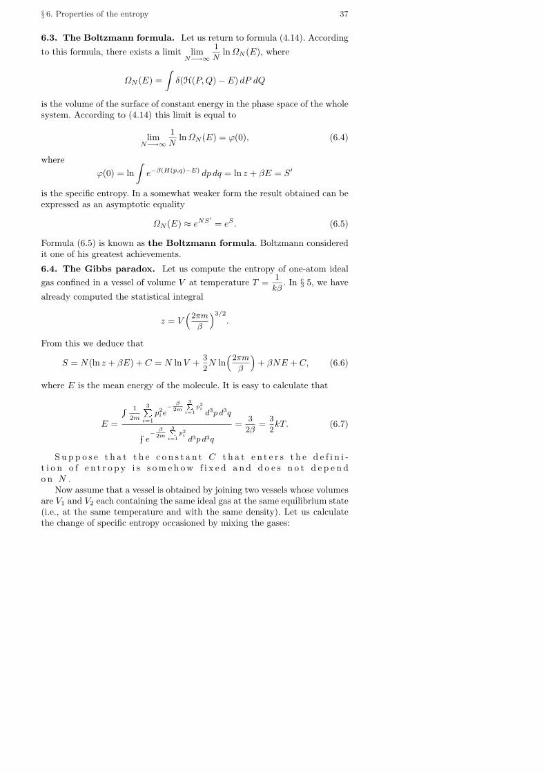
§ 6. Properties of the entropy 37
6.3. The Boltzmann formula. Let us return to formula (4.14). According
to this formula, there exists a limit limN−→∞
1
Nln ΩN (E), where
ΩN (E) =∫
δ(H(P, Q)− E) dP dQ
is the volume of the surface of constant energy in the phase space of the wholesystem. According to (4.14) this limit is equal to
limN−→∞
1
Nln ΩN (E) = ϕ(0), (6.4)
whereϕ(0) = ln
∫e−β(H(p,q)−E) dp dq = ln z + βE = S′
is the specific entropy. In a somewhat weaker form the result obtained can beexpressed as an asymptotic equality
ΩN (E) ≈ eNS′ = eS . (6.5)
Formula (6.5) is known as the Boltzmann formula. Boltzmann consideredit one of his greatest achievements.
6.4. The Gibbs paradox. Let us compute the entropy of one-atom idealgas confined in a vessel of volume V at temperature T = 1
kβ. In § 5, we have
already computed the statistical integral
z = V(
2πm
β
)3/2
.
From this we deduce that
S = N(ln z + βE) + C = N ln V + 3
2N ln
(2πm
β
)+ βNE + C, (6.6)
where E is the mean energy of the molecule. It is easy to calculate that
E =
R 1
2m
3Pi=1
p2i e− β
2m
3Pi=1
p2id3p d3qR
e− β
2m
3Pi=1
p2id3p d3q
= 3
2β= 3
2kT. (6.7)
S u p p o s e t h a t t h e c o n s t a n t C t h a t e n t e r s t h e d e f i n i -t i o n o f e n t r o p y i s s o m e h ow f i x e d a n d d o e s n o t d e p e n do n N .
Now assume that a vessel is obtained by joining two vessels whose volumesare V1 and V2 each containing the same ideal gas at the same equilibrium state(i.e., at the same temperature and with the same density). Let us calculatethe change of specific entropy occasioned by mixing the gases:

38 Ch. 1. The Ensemble of Microscopic Subsystems
1
N∆S = 1
N(S − S1 − S2) = 1
N(N ln V −N1 ln V1 −N2 ln V2) =
N1
Nln V
V1+ N2
Nln V
V2> 0.
Thus, under mixing of identical gases at the same equilibrium state, the meanentropy of one particle increases. This does not make sense since, as a resultof intermixing, we obtain the gas in the same equilibrium state as the initialcomponents. This is the contents of the Gibbs paradox.
To resolve the paradox, we should concede that C must depend on N . Andsince we would like to consider the ideal gas in the vessel of variable volumeV , we must consider it as an ensemble of macroscopic subsystems and setV = Nv, where v is the specific volume that does not depend on N (see. 5.2,5.4). Recall that it is specific volume, not the total volume, that is a physicalcharacteristic of the system.
Set C = −N ln N and use the equality Eβ = 3
2(see (6.7)). As a result, we
obtain an expression of the entropy in terms of the specific volume that doesnot lead to paradoxes:
S = N(ln v + 3
2ln 2πm
β+ 3
2
). (6.8)
The expression in parentheses can be interpreted as the specific entropy. Inconclusion, observe that one can deduce expression (6.8), or rather its version,
with the last summand replaced by 5
2in the following way. In the phase space
of the whole system, consider the function
Φ = e−β(H(P,Q)−E),
where H(P, Q) is the Hamiltonian of the whole system and E = NE is thetotal energy of the system. The integral of Φ over the effective part of thephase space is asymptotically equal to
1
N !
∫Φ dP dQ ≈ eS = eNS′ , (6.9)
where S′ is the expression in the parentheses of (6.6) modified as indicated.We should understand the equality (6.9) as the statement on the existence ofthe limit
S′ = limN−→∞
1
N
(ln 1
N !
∫ΦdP dQ
).
Indeed, set
IN = 1
N !
∫ΦdP dQ = zN
N !eNβE .
Then
1
Nln IN = ln z + βE − ln N !
N= ln V + 3
2ln 2πm
β+ βE − ln N !
N.

§ 7. Analytical appendix to Chapter 1 39
The Stirling formula implies that ln N !
N≈ ln N − 1. Therefore
limN−→∞
1
Nln IN = ln V
N+ 3
2ln 2πm
β+ 5
2= S′.
In our transformations we used the fact that βE = 3
2. Formula (6.9) is re-
markable: It is an exact analogue of the corresponding formula of the quantumstatistical physics and can be obtained from the latter by passing to the limitas h −→ 0, where h is the Planck constant.
7. Analytical appendix to Chapter 1
Let f(x) be locally integrable on (0,∞) and |f(x)| < CxN for x large. ItsLaplace transform is the function
F (t) =
∞∫
0
e−txf(x) dx.
For the Laplace transform, the inversion formula holds:
f(x) = limb−→∞
1
2π
b∫
−b
F (λ+it)e(λ+it)x dt = limb−→∞
1
2πi
λ+ib∫
λ−ib
F (p)epx dp as λ > 0.
(The limit in the right-hand side does not depend on λ).Proof does not differ from the proof of the inversion formula for the Fourier
transform and we will omit it.In order to introduce the Gibbs distribution we have to know the asymp-
totic behavior of the integral
R(N) =
∞∫
−∞ψ(t)eNϕ(t) dt as N −→∞. (7.1)
7.1. Theorem. Let the function ψ(t) be bounded and differentiable, let ϕ(t)be three times continuously differentiable and satisfy the following conditions:
a) ϕ(0) is real; ;b) ϕ′(0) = 0;c) ϕ′′(0) is real and ϕ′′(0) = −α < 0;d) for any δ > 0 and sufficiently large N , we have
∫
|t|>δ
eNRe (ϕ(t)−ϕ(0)) dt <σ
N, where σ = σ(δ).
Then the function R(N) can be expressed, for sufficiently large N , in the form

40 Ch. 1. The Ensemble of Microscopic Subsystems
R(N) =√
π
NαeNϕ(0)
((1 + c(N)√
N
)ψ(0) + b(N)√
N
),
where
|c(N)| ≤ max|t|<δ
ϕ(0)− t2α
t3α,
|b(N)| ≤ supt|ψ(t)|+ max
|t|<δ
∣∣∣ψ(t)− ψ(0)
t
∣∣∣.
If ψ(t) is real, then we have a more convenient estimate of b(N):
|b(N)| ≤ supt|ψ(t)|+ max
|t|<δ|ψ′(t)|.
Proof. Let us present the integral (7.1) as the sum:
∞∫
−∞ψ(t)eNϕ(t) dt =
∫
|t|<δ
ψ(t)eNϕ(t) dt +∫
|t|>δ
ψ(t)eNϕ(t) dt. (7.2)
Let us first estimate the second integral in (7.2):
∣∣∣∣∫
|t|>δ
ψ(t)eNϕ(t) dt
∣∣∣∣ ≤ supt|ψ(t)|
∫
|t|>δ
eNRe ϕ(t) dt =
eNϕ(0) supt|ψ(t)|
∫
|t|>δ
eNRe (ϕ(t)−ϕ(0)) dt ≤ eNϕ(0) supt|ψ(t)| σ
N,
where σ is determined by condition d) of the theorem. We finally see that, forN sufficiently large, we have
∫
|t|>δ
ψ(t)eNϕ(t) dt = eNϕ(0) c1
N, where |c1| ≤ σ sup
t|ψ(t)|. (7.3)
Let us pass to the first integral in (7.2):
δ∫
−δ
ψ(t)eNϕ(t) dt = ψ(0)
δ∫
−δ
eNϕ(t) dt +
δ∫
−δ
[ψ(t)− ψ(0)]eNϕ(t) dt. (7.4)
Thanks to conditions a), b) and c), for a sufficiently small δ and |t| < δ, thefunction ϕ is of the form
ϕ(t) = ϕ(0)− t2α + t3α[ϕ1(t) + iϕ2(t)],
where ϕ1 and ϕ2 are continuous.

§ 7. Analytical appendix to Chapter 1 41
Let us select δ so that, for |t| < δ, we have
1− tϕ1(t) > κ > 0, 1− t
2ϕ1(t) > κ > 0. (7.5)
Let us rewrite the integralδ∫−δ
eNϕ(t) dt:
δ∫
−δ
eNϕ(t) dt = eNϕ(0)
δ∫
−δ
e−Nt2α(1−t[ϕ1(t)+iϕ2(t)]) dt =
eNϕ(0)
δ∫
−δ
e−Nt2α dt + eNϕ(0)
δ∫
−δ
e−Nt2α(eNt3α(ϕ1+iϕ2) − 1
)dt.
It is easy to estimate the first summand:
δ∫
−δ
e−Nt2α dt = 1√Nα
δ√
Nα∫
−δ√
Nα
e−S2dS =
√π
Nα(1 + cN ), (7.6)
where cN = 2∞∫
δ√
Nα
e−S2dS ∼ e−δ2Nα.
In order to estimateδ∫−δ
e−Nt2α(eNt3α(ϕ1+iϕ2) − 1
)dt, observe that
|ea+ib − 1|2 = 1 + e2a − 2ea cos b = 1 + e2a − 2ea + 2ea(1− cos b) =
(1− ea)2 + 4ea sin2 b
2≤ (aea)2 + 4ea sin2 b
2≤
(aea)2 + b2ea ≤ (|a|ea + |b|ea/2)2.
This implies|ea+ib − 1| ≤ |a|ea + |b|ea/2.
Let us use this inequality and (7.5):
∣∣∣∣δ∫
−δ
e−Nt2α(eNt3α(ϕ1+iϕ2) − 1
)dt
∣∣∣∣ ≤δ∫
−δ
e−Nt2αN |t|3α(|ϕ1|eNt3αϕ1+
|ϕ2|eNt3α ϕ12 ) dt ≤
δ∫
−δ
N |t|3α(|ϕ1|+ |ϕ2|)e−Nt2ακ dt ≤
cNα
δ∫
−δ
e−κt2Nα|t|3 dt = cNα
(Nακ)2
δ√
Nκα∫
−δ√
Nκα
e−S2 |S|3 dS =
c
Nακ2(1 + c1(N)), (7.7)

42 Ch. 1. The Ensemble of Microscopic Subsystems
where
c = max|t|<δ
(|ϕ1(t)|+|ϕ2(t)|), c1(N) = 2
∞∫
δ√
Nκα
S3e−S2dS −→ 0 as N −→∞.
Taking into account (7.6) and (7.7) we get
δ∫
−δ
eNϕ(t) dt =√
π
Nα
(1 + a′(N)√
Nα
)eNϕ(0), (7.8)
where
a′(N) ≤ max|t|<δ
(|ϕ1(t)|+ |ϕ2(t)|) + c′(N) ≤√
2max|t|<δ
|ϕ1(t) + iϕ2(t)|+ c′(N) =√
2max|t|<δ
∣∣∣ϕ− ϕ(0) + t2α
t3α
∣∣∣ + c′(N),
and c′(N) −→ 0 as N −→ ∞. For N sufficiently large, we can ignore c′(N)by increasing the estimate of the first summand:
a′(N) ≤ 2max|t|<δ
∣∣∣ϕ− ϕ(0) + t2α
t3α
∣∣∣.
Let us pass to the second integral in (7.4):
∣∣∣∣δ∫
−δ
[ψ(t)− ψ(0)]eNϕ(t) dt
∣∣∣∣ ≤ c1
δ∫
−δ
|t|eNϕ(0)eN(−t2α+t3αϕ1(t)) dt ≤
c1
δ∫
−δ
|t|e−κt2N dteNϕ(0) = c1eNϕ(0) 1− e−κNδ2
κN≤ c1e
Nϕ(0)
κN,
wherec1 = max
|t|<δ
∣∣∣ψ(t)− ψ(0)
t
∣∣∣.
Finally, we see that, for N sufficiently large, we have
δ∫
−δ
ψ(t)eNϕ(t) dt =√
π
NαeNϕ(0)
((1 + a′(N)√
N
)ψ(0) + b′(N)√
N
), (7.9)
where
|a′(N)| ≤ 2max|t|<δ
(|ϕ1(t)|+ |ϕ2(t)|), |b′(N)| ≤ max|t|<δ
∣∣∣ψ(t)− ψ(0)
t
∣∣∣.
Uniting (7.9) and (7.3) we complete the proof of the theorem. ut

Chapter 2
Real gases
8. Physical assumptions
8.1. Properties of interaction. We consider the gas as a collection ofindistinguishable molecules which are massive points with pairwise interactiondescribed by a potential u(x). The gas is confined in a large macroscopic vesselΩ1) and its volume will be denoted by |Ω|. The Hamiltonian of the systemconsisting of M molecules is equal to
H =M∑
i=1
p2i
2m+
∑
1≤i<j≤M
v(qi − qj), (8.1)
where qi = (q(1)i , q
(2)i , q
(3)i ) ∈ Ω and pi = (p(1)
i , p(2)i , p
(3)i ). In order not to
complicate the presentation by inessential details, we will always assume that
u(q) only depends on |q| =√
q(1)2
i + q(2)2
i + q(3)2
i , and
v(q)
= +∞ for |q| ≤ a,
6= ∞ for |q| > a,
= 0 for |q| > b,
6≡ 0 in any interval b1 < |q| < b.
The assumption that v(q) = ∞ for |q| ≤ a physically means that the moleculescannot be at distances smaller than a from each other; that is each of them isconfined in the center of an impenetrable spherical envelope of radius a. It isalso possible to assume that every molecule is a hard ball of radius a
2centered
at qi. The number a
2is sometimes called the radius of the hard core.
The assumption that v(q) = 0 for |q| > b means that the molecules do notinteract if the distance between them is > b. The number b is called the radius1 For example, assume that Ω is a room.

44 Ch. 2. Real gases
v
a b q
Fig. 2 The typical graph of v(q)
of interaction. The numbers a and b are comparable with the actual sizes ofmolecules and are very small from the macroscopic point of view.
The assumption on potential implies an important corollary: There existsa constant C independent of n such that
n∑
i,j=1
v(xi − xj) ≥ nC for any points xi.
8.2. The small and grand ensembles. In order to enter the realm of ideasof statistical physics, we should subdivide the system into weakly interactingsubsystems. Let us discuss how one can do it. Denote the system consideredby C and its phase space by L.
Subdivide the volume Ω into a large number K of macroscopic non-inter-acting subvolumes Ωα
1). Let us consider the volumes Ωα separated from eachother by imaginary partitions impenetrable for the particles but not prevent-ing the interaction of the particles situated on different sides of the partition.Let each volume Ωα contain the same number of particles N . The system thusobtained will be denoted by C ′ and its phase space by L1. The part of the gasconfined in Ωα forms the subsystem needed; we denote it by C1
α. We replacethe initial system by the new system C1 and enumerate the particles of gasagain (there are M = KN of them) and denote by Nα the set of numbers ofthe particles lying in Ωα. The Hamiltonian of the system C1 is of the form
H =∑
Hα + V, where Hα =∑
i∈Nα
p2i
2m+
∑
i,j∈Nαi<j
v(qi − qj),
V =∑
α<β
vα,β , and vα,β =∑
i∈Nαj∈Nβ
v(qi − qj).(8.2)
The systems C1α are not quite identical: The coordinates qiα run over distinct
sets Ωα.We may assume that the interaction between the subsystems C1
α is small.Since, due to the fact that the potential v(q) has a compact support, theenergy of interaction of subsystems
∑vα,β is of the same order of magnitude
1 If Ω is a room, then for Ωα we can take a cube with volume 1 cm3.

§ 8. Physical assumptions 45
as the area of the surface that separates the volumes Ωα, whereas the potentialenergy of the system is proportional to the volume of Ωα and is therefore muchlarger.
Obviously, from the physical point of view, to replace the initial systemC by an auxiliary system C1 is unsatisfactory: the presence of impenetrablewalls changes the properties of the gas confined in Ω: For example, it makesthe large-scale (as compared with the size of Ωα) movements of molecules(such as wind) impossible.
The situation can be corrected by changing the definition of the subsystem.Let us, as earlier, call a portion of the gas confined within Ωα a subsystem;let also think that there are precisely N particles in each Ωα but let us notassume that the particles contained in Ωα are the same ones: The moleculescan exit Ωα and enter Ωα from the other regions of Ω provided the numberof exiting particles is always equal to the number of new arrivals.
The system obtained is said to be a small canonical ensemble. Let usdenote it by C2. We will denote its phase space by L2. The Hamiltonian ofthe small canonical ensemble is obviously of the same form (8.1). Like L1, thephase space L2 is only a part of the total phase space of the initial system.Intuitively it is, however, clear that this part is a main one: The conditionon the constant number of particles in Ωα is satisfied with high accuracy andmeans, essentially, that the density of the gas in all chambers Ωα is the same.
Let us study a relation between the phase space L1 of the auxiliary systemC1 considered earlier and the space L2. The phase space L1 is determined bythe condition
qi ∈ Ωα for i ∈ Nα.
Let g : i −→ g(i) be a permutation of the indices 1, . . . , M . Denote by Lg aregion similar to L1:
qg(i) ∈ Ωα for i ∈ Nα.
Obviously, the phase space of the small canonical ensemble is L2 =⋃
g∈G
Lg
where G is the group of all permutations of the indices 1, . . . , M . Therefore L2
is G-invariant and splits into M !
(N !)K, where M = NK, domains congruent to
L1 and obtained from L1 by the action of G. If F(P, Q) = F(p1, q1, . . . , pM , qM )is a function symmetric with respect to permutations of the pairs (pi, qi), thenintegrals of F over L1 and L2 only differ by a factor:
∫
L2
F dP dQ = M !
(N !)K
∫
L1
F dP dQ.
This implies that the microcanonical means of these functions coincide:RL2
Fδ(H − E) dP dQRL2
δ(H − E) dP dQ=
RL1
Fδ(H − E) dP dQRL1
δ(H − E) dP dQ. (8.3)

46 Ch. 2. Real gases
Thus the statistical properties of the first auxiliary system and the smallcanonical ensemble coincide provided the principle of indistinguishability ofparticles is applicable, i.e., if we only consider the means of symmetric func-tions.
The statistical physics of a real gas always assumes the indistinguishabilityof the particles. Only symmetric functions F(P, Q) exist for us.
Even a more liberal definition of a subsystem is possible. A portion ofgas confined within Ωα is said to be a subsystem without any assumption onthe constant number of the particles in Ωα; this assumption being replacedby a weaker assumption on the constant nature of the microcanonical meannumber of particles in Ωα. The collection of such subsystems is called a grandcanonical ensemble. The phase space of the grand canonical ensemble L3 obvi-ously contains the space L2 of the small canonical ensemble but is, obviously,contained within the phase space L of the initial system.
In conclusion, observe that the real gas is an ensemble of macroscopic sub-systems. Unlike the systems studied in Chapter 1, for which the presence ofone large number — the number of subsystems in a system — was a character-istic feature, the real gas is characterized by two large numbers: The numberK (K > 105) of subsystems in the system and the number N (N > 1020) ofparticles in each subsystem.
Obviously, only the quantities obtained as a result of two consecutive pas-sages to the limits (as K −→ ∞ and N −→ ∞) may possess a physicalinterpretation. Both limit processes are called thermodynamic ones and bothprocesses assume that the density of the gas remains constant.
The first passage to the limit
K −→∞, |Ωα| = const, N = const,
is analogous to the thermodynamic limit considered in Chapter 1. It turns themicrocanonical distribution in the small canonical ensemble into the Gibbsdistribution for the subsystem.
The second limiting process
N −→∞, such that N
|Ωα| = const,
is indigenous for the real gases and does not appear in the study of ensemblesof microscopic subsystems.
9. The Gibbs Distribution in the Small CanonicalEnsemble
9.1. Step one. At the moment, no rigorous, in the modern sense of thisword, deduction of the Gibbs distribution in this situation is known, andtherefore we will confine ourselves to heuristic arguments.

§ 9. The Gibbs Distribution in the Small Canonical Ensemble 47
First of all, assume that for the Hamiltonian (8.1) the ergodic hypothesisis applicable. This implies that the mean with respect to time of any physicalquantity is equal to the mean over the surface of constant energy1) (see § 1).
F =R
Fδ(H − E) dP dQRδ(H − E) dP dQ
, (9.1)
where H is the Hamiltonian (8.1), P = (p1, . . . , pM ), Q = (q1, . . . , qM ).We assume that the principle of indistinguishibility of the particles is appli-
cable, i.e., apply formula (8.1) only to the functions F symmetric with respectto permutations of the pairs (pi, qi).
Let nα be the number of molecules in the cell Ωα and K the number ofcells in Ω and let χα(q) be the characteristic function of the cell Ωα. Observethat
1 =K∑
α=1
χα(q) =M∏
i=1
( K∑α=1
χα(qi))
=∑
χα1(q1) . . . χαM(qM ). (9.2)
Using identity (9.2) and the symmetry of F we find that the numerator in (9.1)is equal to
∑ M !
n1! . . . nK !
∫F(P, Q)χα1(q1) . . . χα1(qn1)χα2(qn1+1) . . . χα2(qn1+n2) . . .
χαK(qn1+n2+···+nK−1+1) . . . χαK
(qn1+n2+···+nK)δ(H − E) dP dQ. (9.3)
It is natural to assume that the values of the individual integrals in (9.3) donot differ much from each other. Therefore the maximal summand in (9.3) isthe one with the greatest factor. To find it, we proceed in the same way asin the deduction of the Gibbs distribution in § 3. Taking into account thatbetween the numbers nα there exists only one relation, namely
∑nα = M ,
we set
f = ln M !
n1! . . . nK !+ µ
∑
i
ni = ln M !−∑
r
nr(lnnr − 1) + µ∑
r
nr.
This implies that1 Unlike the ensemble of the microscopic subsystems, the theorem on ergodicity
of the total system justifies now the passage from the mean with respect totime to the microcanonical mean (9.1). However, even now, the theorem on theergodicity of the individual system (i.e., the system with a fixed function H)seems to be not needed since we do not know the precise value of the potentialof the intermolecular interaction anyway. The theorem on density of the set ofergodic dynamical systems with Hamiltonian (8.1), in the set of all systems ofthis type appears to be more natural. The arguments given in § 2 in a similarsituation indicate that such a system would be sufficient, apparently, to justifythe passage from the mean with respect to time to the microcanonical mean.

48 Ch. 2. Real gases
∂f
∂ni= − ln ni + µ. (9.4)
Equating the expression (9.4) to zero we see that ni = eµ, i.e., the maximumis attained when all the ni are equal: ni = N for all i. The denominatorin (9.1) is obtained from the numerator as we set F ≡ 1. Therefore it alsoadmits a representation in the form of a sum similar to (9.3). Let us replacethe numerator and the denominator by the maximal summands and denotetheir ratio by F1. After simplification we get
F1 =RFχα1(q1) . . . χα1(qN ) . . . χαK (q(K−1)N+1) . . . χαK (qKN )δ(H − E) dP dQRχα1(q1) . . . χα1(qN ) . . . χαK (q(K−1)N+1) . . . χαK (qKN )δ(H − E) dP dQ
=RL1
Fδ(H − E) dP dQRL1
δ(H − E) dP dQ, (9.5)
where L1 is the phase space of the auxiliary system C1 described in § 8.We should prove that in the thermodynamic limit, that is as
|Ω| −→ ∞, K −→∞, M −→∞ provided |Ωα| = const, |Ω|M
= const,(9.6)
we havelim F = lim F1. (9.7)
The equality (9.7) is a justification for the replacing of the initial systemby the auxiliary system C1 described in § 8 or, which is the same thanksto identity (8.3), by a small canonical ensemble. This equality (9.7) is nothowever, rigorously proved at the moment so we will accept it as a hypothesis.
9.2. Step two. Let us transform the right-hand side of formula (9.5). Firstof all, we will apply it not to arbitrary functions F but to integrable functionsof the form
F(P,Q) = f(p1, q1, . . . , pn, qn)χ0(q1) . . . χ0(qn) + . . .M !
n!(M − n)!
. (9.8)
The dots stand for the summands obtained from the 1-st one under arbitrary
permutations of the pairs (pi, qi). There are M !
n!(M − n)!distinct summands
altogether. Apart from the inequality n ≤ N , there is no relation between nand N . (In what follows we are interested in the limit as N −→∞ whereas nremains constant.)
The numerator in the right-hand side of (9.5), after substituting the func-tion F of the form (9.8) in it, takes the form∫
L1
f(p1, q1, . . . , pn, qn)δ(H1 + . . . + HK + V − E) dP dQ, (9.9)

§ 9. The Gibbs Distribution in the Small Canonical Ensemble 49
where Hα and V are of the form (8.2). Hereafter we assume, for convenience,that the set N0 consists of the first N positive integers. We visualize thevolumes Ωα as small cubes centered at points aα; let Ω0 be a cube centeredat the origin. Perform a coordinate change qi = qi − aα for i ∈ Nα, where Nα
is a set of indices. Observe that
Hα(p, q) =∑
i∈Nα
p2i
2m+
∑
i,j∈Nαi<j
v(qi − qj) =∑
i∈Nα
p2i
2m+
∑
i,j∈Nαi<j
v(qi − qj).
As a result of the above change, the integral (9.9) turns into an integral overthe cube Ω0. Having denoted qi by qi again, we see that the integral (9.9) isequal to
∫f(P0, Q0)δ
( K∑α=0
H(Pα, Qα) +∑
0≤α<β≤K
vαβ − E
) ∏α
dPα dQα, (9.10)
where Pα = pi | i ∈ Nα, Qα = qi | i ∈ Nα, qi ∈ Ω0 and where
vαβ =∑
i∈Nαj∈Nβ
v(qi − qj + aα − aβ). (9.11)
The potential of interaction vαβ is nonzero only if aα and aβ are the centersof neighboring cubes. Even in this case, vαβ 6= 0 only if the points qi +aα andqj +aβ are sufficiently close to each other. Therefore we may assume that theinteraction is “small”. Ignoring it we replace the mean (9.5) by the new mean
F2 =
Rf(P0, Q0)δ
KP
α=0
H(Pα, Qα)− E
QdPα dQαR
δ
KP
α=0
H(Pα, Qα)− E
QdPα dQα
. (9.12)
It is natural to assume that under the thermodynamic limit (9.6) we have
limF2 = lim F1. (9.13)
Like equality (9.7), the equality (9.13) is not rigorously proved at themoment and this is our next hypothesis. Now observe that the equation (9.12)led us to the situation when the Gibbs distribution takes place. Taking intoaccount (9.7) and (9.13) we obtain as a result of the 1-st thermodynamicpassage to the limit that
F =R
f(p1, q1, . . . , pn, qn)e−βH(p1,q1,...,pN ,qN ) dNp dNqRe−βH(p1,q1,...,pN ,qN ) dNp dNq
, (9.14)
where F is a function of the form (9.8) and
H =N∑
i=1
p2i
2m+
∑
1≤i<j≤N
v(qi − qj), where qi ∈ Ω0,
is the energy operator of the subsystem. The parameter β is determined, asusual, from the equation

50 Ch. 2. Real gasesRHe−βH dNp dNqRe−βH dNp dNq
= E. (9.15)
This completes the deduction of the Gibbs distribution in the small canonicalensemble.
9.2.1. Remarks. 1) The fact that eq. (9.14) yields the Gibbs distribution inthe small canonical ensemble, i.e., that all subsystems determined by volumesΩα contain the same number of particles, follows directly from the deductionof eq. (9.14).
2) Eq. (9.14) is true only asymptotically as N −→ ∞ provided N
|Ω0| = γ;
the right-hand side of (9.14) is equal to the microcanonical mean of F sincethe interaction between subsystems becomes small and we can ignore it withsufficient justification only as |Ωα| −→ ∞. This is precisely the reason whythe number of arguments of the function f is taken to be equal to n —the number having nothing to do with the total number N of particles inthe system: Otherwise we would have to change, as N grows, the number ofarguments of f which is a bother.
10. The correlation functions in the small canonicalensemble
10.1. Main definitions. Let a subsystem satisfying the Gibbs distributionbe situated in a vessel Ω of volume |Ω|. Observe that the density of the Gibbsdistribution in the small canonical ensemble is a product
ρ(p1, q1, . . . , pN , qN ) = ρp(p1, . . . , pN )ρq(q1, . . . , qN ), (10.1)
where ρp is the density of the distribution in the space of momenta which isa Gaussian one and does not depend on the potential of the interaction andwhere ρq is the density of the distribution in the space of positions which isequal to
ρq = e−β
Pi<j
v(qi−qj)
zN, where zN =
∫
qi∈Ω
e−β
Pi<j
v(qi−qj)
dNq. (10.2)
Since the factor ρp is particularly simple, the function ρq, as well as the meanvalues of the functions that do not depend on p, are of greatest interest.
Consider the function
F (q) = f(q1, . . . , qn) + . . . , (10.3)
where f is an integrable function, n a fixed number having no relation withN , and the sum in (10.3) is obtained from the first summand by permuting
the qi (altogether N !
n!(N − n)!distinct summands).

§ 10. The correlation functions in the small ensemble 51
Since f only depends on the coordinates of a finite number of particles, themean of F over the Gibbs distribution should possess a physical interpretation,i.e., we may expect that the thermodynamic limit of the mean values exists.Consider the mean value F in more detail. By (10.1), (10.3) we have∫
F (q)ρ(p, q) dNp dNq =∫
F (q)ρq(q) dNq = N !
n!(N − n)!
∫f(q)ρn,N (q) dnq,
(10.4)where
ρn,N = |Ω|nR
e−β
P1≤i<j≤N
v(qi−qj)
dqn+1 . . . dqN
zN. (10.5)
The function ρn,N (q1, . . . , qn) is called n-particle correlation function, (pre-limit one). Observe that
N !
n!(N − n)!|Ω|−n = N(N − 1) . . . (N − n + 1)
n!Ω−n
has a limit equal to γn
n!as N −→∞ provided N
|Ω| = γ = const.
According to the above, we may expect the presence of thermodynamiclimit in the left-hand side of (10.4), and hence in the right-hand side, andtherefore the limit of the function ρn,Ω . Assuming that such a limit exists,denote the limit function by ρn. Thus, the thermodynamic limit of the meanvalues of F is equal to
F = γn
n!
∫f(q1, . . . , qn)ρn(q1, . . . , qn) dnq. (10.6)
Let h be an arbitrary vector whose length does not exceed the radius ofinteraction b. Observe that
ρn,Ω(q1 + h, . . . , qn + h) = ρn,Ω(q1, . . . , qn) + ∆n,Ω ,
where ∆n,Ω is obtained by integrating the right-hand side of (10.5) over thedomain in which at least one variable qi is distant from the boundary of Ωnot further than b. Therefore we expect that lim
|Ω|−→∞∆n,Ω = 0 and the limit
correlation functions satisfy
ρn(q1 + h, . . . , qn + h) = ρn(q1, . . . , qn). (10.7)
The relation (10.7) being true for vectors h of small length remains, obviously,true for arbitrary vectors.
We often have to consider mean values of functions of the form (10.3) forwhich f is not, however, integrable but only satisfies (10.7), i.e., only dependson the mutual disposition of molecules but not on the location of the wholeconfiguration, as total, in space.

52 Ch. 2. Real gases
The same arguments as above indicate that, in this case, it is natural toexpect that the thermodynamic limit of the function F
|Ω| exists and is equal
toγn
n!
∫f(q1, . . . , qn)ρn(q1, . . . , qn) dq1 . . . dqn−1.
In other words, as |Ω| −→ ∞, N −→∞ provided N
|Ω| = γ, the mean value F
is asymptotically equal to
F ≈ |Ω|γn
n!
∫f(q1, . . . , qn)ρn(q1, . . . , qn) dq1 . . . dqn−1. (10.8)
10.2. The asymptotics of the statistical integral. The thermody-namic potential. Leaving aside for a moment the question of existence ofthe limit correlation functions ρn let us discuss eqs. (10.6)–(10.8). First of all,observe that
−∂ ln zN
∂β= 1
zN
∫ ∑v(qi − qj)e
−βPi<j
v(qi−qj)
dNq =
N(N − 1)
2|Ω|−2
∫v(q1 − q2)ρ2,N (q1, q2) dq1 dq2. (10.9)
If everything said above holds, then the asymptotics of the integral in theright-hand side of (10.9) is equal to
|Ω|∫
v(q)ρ(q) dq,
where, for brevity, we set ρ(q) = ρ2(q1, q2) and q = q1 − q2. Therefore we
expect that as |Ω| −→ ∞ (so that N
|Ω| = γ) we should have
− 1
|Ω|∂ ln zN
∂β= γE(β, γ) + O(1), E(β, γ) =
∫v(q)ρ(q) dq, (10.10)
where E(β, γ) is the mean potential energy.Observe that zN = |Ω|N at β = 0. Therefore integrating (10.10) from 0 to
β we find that
− 1
|Ω| (ln zN −N ln |Ω|) = γ
β∫
0
E(S, γ) dS + O(1). (10.11)
Taking into account that |Ω| = N
γ, we deduce from (10.11) that
1
|Ω| lnzNN
γ
N= −γ
β∫
0
E(S, γ) dS + O(1).

§ 10. The correlation functions in the small ensemble 53
Taking into account the Stirling formula N ! ∼(
N
e
)N
, the above expres-sion finally yields
limN−→∞
1
Nln zN
N != F (β, γ), F (β, γ) = −
β∫
0
E(S, γ) dS − γ−1 ln γ
e. (10.12)
Thus, assuming the existence of the second limit correlation function, we de-duce the existence of the limit (10.12). The limit function F (β, γ) is called thethermodynamic potential of the small canonical ensemble. At present no in-dependent proofs of the existence theorems for the thermodynamic potentialand the limit correlation functions are known. The existence of the thermo-dynamic potential is proved for all β ≥ 0, γ ≥ 0 and the existence of thecorrelation functions is proved only in a region1) of all possible values of β, γ.
In what follows, we will give the detailed proofs of analogous theorems forthe grand canonical ensemble. Concerning the small canonical ensemble, dueto much greater difficulty of the proofs, we will only sketch them and giveheuristic arguments.
10.3. Pressure. Let us express the pressure in terms of 2-nd correlationfunction. We’ll use the definition of the pressure given in § 5. According tothis definition, the pressure of the gas confined in a finite volume is equal to
pΩ = 1
β
∂ ln zN
∂|Ω| . (10.13)
In order to study the behavior of pΩ under the thermodynamic limit,suppose that Ω is a cube with side l and perform the change qi = lxi. In newvariable, we have
zN = |Ω|N∫
xi∈I
e−β
Pi<j
v(lxi−lxj)
dNx,
where I is the unit cube.Observe that |Ω| = l3 and so
dl
d|Ω| = 1
3
l
|Ω| ,∂ ln zN
∂|Ω| = ∂ ln zN
∂l
1
3
l
|Ω| .
Setqi = (q1
i , q2i , q3
i ), v′α(q) = ∂
∂qαv(q).
1 If the system is subject to phase transitions, the limit correlation functions mayindeed be undefined for the values of β, γ at which the phase transition takesplace. Observe, however, that the existence theorem is proved for the domain ofvalues of β, γ much more narrow than the one for which such existence is naturalto expect.

54 Ch. 2. Real gases
Let us find ∂
∂|Ω|zN :
∂zN
∂|Ω| = N |Ω|N−1
∫
xi∈I
e−β
Pi<j
v(lxi−lxj)
dNx+
|Ω|N 1
3
l
|Ω| (−β)∫
xi∈I
∑
i<j,α
(xαi − xα
j )v′α(lxi − lxj)e−β
Pi<j
v(lxi−lxj)
dNx =
N |Ω|N−1
∫
xi∈I
e−β
Pi<j
v(lxi−lxj)
dNx−
βN(N−1)
2 · 3 · l|Ω|N−1
∫
xi∈I
∑α
(xα1 − xα
2 )v′α(lx1 − lx2)e−β
Pi<j
v(lxi−lxj)
dNx =
N
|Ω|zN − βN(N − 1)
6|Ω|∑
qi∈Ω
∑α
(qα1 − qα
2 )v′α(qα1 − qα
2 )e−β
Pi<j
v(qi−qj)
dNx.
We see that
pΩ = 1
β
∂ ln zN
∂|Ω| = 1
βz−1N
∂zN
∂|Ω| =
= N
β|Ω| −N(N − 1)
6|Ω||Ω|2∫ ∑
α
(qα1 − qα
2 )v′α(q1 − q2)ρ2,N (q1, q2) dq1 dq2.
Therefore assuming that the second correlation function exists, we see thatthere exists a thermodynamic limit of pΩ equal to
p = γ
β− γ2
6
∫ ∑α
qα ∂v
∂qαρ(q) dq. (10.14)
The function∑α
qα ∂v
∂qαis well-known in mechanics; it is called the virial of
force. Thus, the pressure becomes closely connected with the mean of thevirial of force of intermolecular interaction.
In conclusion, let us give an expression of the pressure in terms of thethermodynamic potential. Due to (10.12), for N and |Ω| large, we have
zN
N !≈ e
NF(β, N|Ω|
).
ThereforepΩ = 1
β
∂ ln zN
∂|Ω| ≈ −γ2
β
∂F
∂γ.
The right-hand side of this formula gives a thermodynamic limit of pΩ :
p = lim|Ω|−→∞
pΩ = −γ2
β
∂F
∂γ. (10.15)

§ 11. The Bogolyubov equations 55
11. The Bogolyubov equations
11.1. A deduction of the equations. The correlation functions of thesmall canonical ensemble are little adjusted to rigorous study. The correlationfunctions of the grand canonical ensemble are more appropriate.
In this section, we give a brief sketch of a heuristic study of correlationfunctions of the small canonical ensemble. The central role here is played bythe Bogolyubov equations.
Set
u(x1, . . . , xn) = e−β
P1≤i<j≤n
v(xi−xj)
, where xi = (xi,1, xi,2, xi,3). (11.1)
Observe that
∂u
∂xi,ε= −β
n∑
k=1
∂v(xi − xk)
∂xi,εu(x1, . . . , xn), for ε = 1, 2, 3. (11.2)
Let i ≤ s. Let us integrate (11.2) over xs+1, . . . , xn and multiply by |Ω|szn
. Weget
∂(x1, . . . , xs)
∂xi,ε= −β|Ω|s
zn
∫ n∑
k=1
∂v(xi − xk)
∂xi,εe−β
P1≤i<j≤n
v(xi−xj)
dxs+1 . . . dxn =
− β
s∑p=1
∂v(xi − xp)
∂xi,ερs,n(x1, . . . , xs)−
β|Ω|szn
n∑
k=s+1
∫∂v(xi − xk)
∂xi,εe−βv(xi−xj) dxs+1 . . . dxn =
− β
s∑p=1
∂v(xi − xp)
∂xi,ερs,n(x1, . . . , xs)−
β|Ω|szn
(n− s)∫
∂v(xi − xs+1)
∂xi,εe−β
P1≤i<j≤n
v(xi−xj)
dxs+1 . . . dxn =
− β
s∑p=1
∂v(xi − xp)
∂xi,ερs,n(x1, . . . , xs)−
β(n− s)
Ω
∫∂v(xi − xs+1)
∂xi,ερs+1,n(x1, . . . , xs+1) dxs+1.
Therefore we have obtained a system of interrelated integro-differential equa-tions for ρs,n (s = 1, 2, . . . , n) called the chain of Bogolyubov equations:
∂ρs,n
∂xi,ε= −β
s∑p=1
∂v(xi − xp)
∂xi,ερs,n − β
(n− s)
Ω
∫∂v(xi − xs+1)
∂xi,ερs+1,n dxs+1.
(11.3)

56 Ch. 2. Real gases
Taking into account that (n− s)
Ω−→ γ we can formally pass to the ther-
modynamic limit and obtain the equation for correlation functions in the limitcase:
∂ρs
∂xi,ε= −β
s∑p=1
∂v(xi − xp)
∂xi,ερs − βγ
∫∂v(xi − xs+1)
∂xi,ερs+1 dxs+1. (11.4)
The function
ρs,n(x1, . . . , xs) = eβP
i≤j≤s
v(xi−xj)
ρs,n(x1, . . . , xs) (11.5)
is often more convenient. The limit function ρs is similarly defined. For thefunctions ρs, we deduce from (11.4) the equations
∂ρs
∂xi,ε= −βγ
∫∂v(xi − xs+1)
∂xi,εe−βPj
v(xj−xs+1)
ρs+1 dxs+1. (11.6)
Similarly, from (11.3) we can derive the equations for ρs,n but we will not givehere their explicit form.
11.2. Extension with respect to degrees of density. Equations (11.4)or, which is the same (11.6)), are convenient for deducing formal expansions ofthe functions ρn in power series in γ. In order to obtain these expansions, weshould complement the equations (11.4) (or (11.6)) by the boundary condition
lim ρn(x1, . . . , xn) = 1 as |xi − xj | −→ ∞,
lim ρn(x1, . . . , xn) = 1 as |xi − xj | −→ ∞. (11.7)
An (heuristic) deduction of conditions (11.7) will be given at the end of thissection.
Let us find the 0-th and the first terms of the power series of expansion ofρn in powers of γ:
ρn = ρ(0)n + γρ(1)
n + O(γ2), where ρ(0)n = 1.
Indeed, eq. (11.6) implies ∂
∂xi,ερ(0)n = 0, and hence ρ
(0)n = const. Let us
use (11.7) and pass to the limit at each term of the expansion of ρn in powersof γ. Since (11.7) holds identically with respect to γ, we have
lim|xi−xj |−→∞
ρ(0)n = 1, lim
|xi−xj |−→∞ρ(s)
n = 0 for s > 0. (11.8)
Taking into account that ρ(0)n = const, the first relation of (11.8) yields the
result desired: ρ(0)n = 1.
For ρ(1)n , we derive from (11.6) the equation

§ 11. The Bogolyubov equations 57
∂ρ(1)n
∂xi,ε= −β
∫∂v(xi − xn+1)
∂xi,εe−βPj
v(xj−xn+1)
dxn+1 =∫
∂
∂xi,εe−βPj
v(xj−xn+1)
dxn+1.
Here the derivative cannot be interchanged with the integral sign since thefunction
e−βPj
v(xj−xn+1)
is not integrable with respect to xn+1. Set
e−βv(x) = 1 + f(x). (11.9)
Then
e−β
nPj=1
v(xj−xn+1)
=n∏
j=1
(1 + f(xj − xn+1)) = 1 +n∑
j=1
f(xj − xn+1)+
∑
j1<j2
f(xj1 − xn+1)f(xj2 − xn+1) + . . .
∂ρ(1)n
∂xi,ε=
∫∂
∂xi,ε
(1 +
∑f(xj − xn+1)+
+∑
j1<j2
f(xj1 − xn+1)f(xj2 − xn+1) + . . .)
dxn+1 =
∫∂
∂xi,ε
( ∑
j1<j2
f(xj1 − xn+1)f(xj2 − xn+1) + . . .)
dxn+1 =
∂
∂xi,ε
∫ ( ∑
j1<j2
f(xj1 − xn+1)f(xj2 − xn+1) + . . .)
dxn+1.
Observe that the assumptions on v(x) imply that f(x) has a compact support.The integrand in the last integral is equal to
u(x1, . . . , xn | xn+1) =∑
j1<j2
f(xj1 − xn+1)f(xj2 − xn+1) + . . . =
e−βP
v(xj−xn+1) − 1−∑
f(xj − xn+1), (11.10)
it is integrable with respect to xn+1, and therefore in the last equality, we caninterchange the partial derivative and the integral sign.
Thus,
ρ(1)n =
∫u(x1, . . . , xn | xn+1) dxn+1 + Cn, (11.11)
where u is defined from eq. (11.10).In order to determine Cn, let us use eq. (11.8) at s = 1. Integrating the
first summand in (11.10) we see that

58 Ch. 2. Real gases
∫f(x1 − xn+1)f(x2 − xn+1) dxn+1 =
∫f(y)f(x2 − x1 − y) dy. (11.12)
Since f(x) has a compact support, it follows that the integral (11.12) vanishesfor sufficiently large |x1 − x2|. The integrals of the remaining summands en-tering (11.10) are similarly studied. Therefore the first summand in (11.11)vanishes for sufficiently large |xi − xj |. Hence, Cn = 0. Finally,
ρ(1)n =
∫ (e−βPj
v(xj−xn+1) − 1−∑
j
f(xj − xn+1))
dxn+1. (11.13)
In principle, one can similarly find all the functions ρ(s)n but the corresponding
formulas are very cumbersome for s > 1.Let us prove relations (11.7). To this end, let us find, starting from (11.6),
the expansion of ρn in power series in γ without appealing to (11.7). The func-tions obtained will be denoted by ˜ρn to distinguish them from the solutions of
the system (11.6) that takes (11.7) into account. For ˜ρ(0)
n and ˜ρ(1)
n repeatingthe above arguments we find that
˜ρ(0)
n = C(0)n = const, ˜ρ
(1)
n = C(0)n+1ρ
(1)n + C(1)
n .
One can easily establish by the induction that
˜ρ(s)
n = C(0)n+sρ
(1)n + C
(1)n+s−1ρ
(s−1)n + . . . + C(s)
n . (11.14)
Eq. (11.14) implies that ˜ρ(s)
n has a limit as |xi − xj | −→ ∞ and this limit isequal to C
(s)n . Therefore the function ˜ρn has a limit as |xi − xj | −→ ∞ and
this limit is equal to∑
jsC(s)n = a(γ). Let the correlation function be related
to ˜ρn as followsρn = e−β
Pv(xi−xj) ˜ρn.
In this caselim ρn = lim ˜ρn = a(γ) as |xi − xj | −→ ∞.
Thereforelim
L−→∞1
Ln
∫
|xi|<L
ρn(x1, . . . , xn) dnx = a(γ).
Since ρn = limN−→∞
ρn,N , the relation
limL−→∞
1
Ln
∫
|xi|<L
ρn,N (x1, . . . , xn) dnx = a(γ)
should also be satisfied. However, the expression under the limit sign is identi-cally equal to 1. Therefore: a(γ) ≡ 1, relations (11.7) hold, C
(s)n = 0 for s > 0,
and C(0)n = 1.

§ 12. The Gibbs distribution in the grand ensemble 59
12. The Gibbs distribution in the grand canonicalensemble
12.1. Transforming the microcanonical mean. In the same way wedid this in § 9, consider a system of M particles confined in the volume Ωpartitioned into cells Ωα, where α = 1, 2, . . . , K. Let
F(x1, . . . , xM ) =P
f(x1, . . . , xs)χ1(x1) . . . χ1(xs) + . . .M !
s!(M − s)!
, (12.1)
where χ1(x) is the characteristic function of Ω1 and where dots denote, asusual, the sum of summands obtained from the first one by the permutationof the xi.
As in § 8, the problem is to rearrange the microcanonical mean of F (withrespect to the system considered). Let us subdivide the volume Ω into K1
cells ωσ, where |ωσ| = |ω|, each of which consists, in turn, of K2 subcells Ωα
so that K = K1 · K2 and |ω| = K2|Ω1|. Consider the first thermodynamiclimit as K −→∞ |Ω| −→ ∞ whereas Ωα remains constant.
Let us perform the passage to the limit in two steps: First let |Ω| and K1
tend to ∞ whereas the intermediate volumes ωσ remain fixed, then tend ωσ
and K2 to ∞. Denote by ω1 the intermediate subvolume containing Ω1.As a result of the first step of the passage to the thermodynamic limit,
we arrive at the situation considered in § 8: The microcanonical mean of thefunction F in the limit as K1 −→ ∞ and |Ω| −→ ∞ whereas M
|Ω| = const is
equal to the canonical mean over the small canonical ensemble determined bythe volume ω1:
F = 1
zn
∫
xi∈ω
f(x1, . . . , xs)e−β
Pi<j<n
v(xi−xj)
χ1(x1) . . . χ1(xs) dx1 . . . dxn.
(12.2)
In formula (12.2), we have introduced, for brevity: n = M
K1is the number
of particles in ωσ, in particular in ω1; ω = ω1, and χ(x) = χ1(x) is thecharacteristic function of the subvolume Ω1 ⊂ ω. Now, we have to investigatethe integral (12.2) as n −→∞ provided n
|ω| = γ.
Let ω′ be the complement to Ω1 in ω. Further, at each point of Ω1, weplace the center of the ball of radius b, where b is the radius of intermolecularinteraction. Let Ω1be the union of all these balls. Obviously, Ω1 ⊂ Ω1. Let ω′
be the complement to ω in Ω1. The particles lying in ω′ and Ω1 do not interactsince |x− y| > b for x ∈ Ω1 and y ∈ ω′, and therefore v(x− y) = 0. One canconsider the complement to Ω1 in Ω1 as the partition whose thickness is equalto the radius of interaction. Let χ(x) be the characteristic function of Ω1, andso χ′(x) = 1− χ(x) is the characteristic function of ω′. Using the identity

60 Ch. 2. Real gases
1 =n∏
i=1
(χ(xi) + χ′(xi)) =n∏
i=1
χ′(xi) +∑
j
(∏′
jχ(xi))χ(xj)+
∑
j1<j2
(∏′′
j1,j2χ′(xi))χ(xj1)χ(xj2) + . . . , (12.3)
where∏(k)
j1...jkχ′(xi) denotes the product of the χ′(xi) over all i except
i = j1, . . . , jk, we rewrite the expression for zn(ω) as follows:
zn(ω) =∫
xi∈ω
n∏1
(χ(xi) + χ′(xi))e−βP
v(xi−xj) dx1 . . . dxn =
zn(ω′) + n
∫
xi∈ω′ as i>1x1∈Ω1
e−βP
v(xi−xj) dx1 . . . dxn+
n(n− 1)
2!
∫
xi∈ω′ as i>2x1,x2∈Ω1
e−βP
v(xi−xj) dx1 . . . dxn + . . . (12.4)
Now, let us replace the exact equality (12.4) by an approximate one which dif-fers from (12.4) in that ω′ is replaced by ω′. In view of the fact that v(x−y) = 0for x ∈ Ω1 and y ∈ ω′, we have
zn(ω) ≈ zn(ω′) + n|Ω1|zn−1(ω′) + n(n− 1)
2!z2(Ω1)zn−2(ω′) + . . . (12.5)
The approximate equality (12.5) is the more precise the greater the vol-umes ω, ω′ and Ω1.
Consider the ratio zn−1(ω′)
zn(ω′)for n large. Setting
limn−→∞
1
nln zn
n!= F (γ, β), where γ = n
|ω′| ,
we see that
zn−1(ω′)
zn(ω′)≈ (n− 1)!e
(n−1)F
n−1|ω′| ,β
n!e
nF
n|ω′| ,β
≈ 1
ne(n−1)F
(n−1|ω′| ,β
)−nF
(n|ω′| ,β
)≈
1
ne(n−1)
(− 1|ω′|
∂F∂γ
(n|ω′| ,β
))−F
(n|ω′| ,β
)= 1
ne−(
F (γ,β)+γ ∂F∂γ
(γ,β)
).
Recall that γ = n
|ω′| ≈n− 1
|ω′| .
Setβµ = −
(F (γ, β) + γ
∂F
∂γ(γ, β)
), where ζ = eβµ. (12.6)

§ 12. The Gibbs distribution in the grand ensemble 61
The quantities µ and ζ are called the chemical potential and activity, respec-tively. We see that
zn−k
zn= zn−1
zn· zn−2
zn−1. . .
zn−k
zn−k+1≈ ζk 1
n(n− 1) . . . (n− k + 1)= ζk (n− k)!
n!.
(12.7)We finally have
zn(ω) ≈ zn(ω′)∞∑0
ζk
k!zk(Ω1) (z0 = 1, z1 = |Ω1|). (12.8)
Let us pass to the integral in the numerator of (12.2) and transform it in thesame way we have transformed zn:
∫
xi∈ω
f(x1, . . . , xs)χ(x1) . . . χ(xs)n∏
s=1
(χ(xi)+χ′(xi))e−βP
v(xi−xj) dx1 . . . dxn =
∫
xi∈Ω1 for i≤sxi∈ω′ for i>s
f(x1, . . . , xs)e−βP
v(xi−xj) dx1 . . . dxn+
(n− s)∫
xi∈Ω1 for i≤s+1xi∈ω′ for i>s+1
f(x1, . . . , xs)e−βP
v(xi−xj) dx1 . . . dxn+
(n−s)(n−s−1)
2!
∫
xi∈Ω1 for i≤s+2xi∈ω′ for i>s+2
f(x1, . . . , xs)e−βP
v(xi−xj) dx1 . . . dxn + . . .
Having replaced the integral over ω′ by the integral over ω′ we get an approx-imate equality
∫f(x1, . . . , xs)χ(x1) . . . χ(xs)e
−βP
i<j≤n
v(xi−xj)
dx1 . . . dxn ≈∫
xi∈Ω1
f(x1, . . . , xs)e−β
Pi<j≤n
v(xi−xj)
dx1 . . . dxnzn−s(ω′)+
(n−s)∫
xi∈Ω1
f(x1, . . . , xs)e−β
Pi<j≤s+1
v(xi−xj)
dx1 . . . dxs+1zn−s−1(ω′) + . . .
Let us use relation (12.7):

62 Ch. 2. Real gases
∫
ω
f(x1, . . . , xs)χ(x1) . . . χ(xs)e−βP
v(xi−xj) dx1 . . . dxn ≈
(n− s)!
n!z(ω
′)∫
Ω1
f(x1, . . . , xs)×
×( ∞∑
k=0
ζs+k
k!
∫
Ω1
e−β
Pi<j≤k+s
v(xi−xj)
dxs+1 . . . dxs+k
)dx1 . . . dxs.
For the mean value (12.2), we get the following final approximate expression
F = 1
s!
∫
Ω1
f(x1, . . . , xs)rs,Ω1(x1, . . . , xs) dsx, (12.9)
where
rs,Ω1(x1, . . . , xs) = 1
Ξ
∑ ζs+k
k!
∫
Ω1
e−β
Pi<j≤s+k
v(xi−xj)
dxs+1 . . . dxs+k, (12.10)
Ξ =∞∑
k=0
ζk
k!zk(Ω1). (12.11)
It is natural to expect that the approximation (12.9) is such that the limitof the right-hand side of (12.9) as |Ω1| −→ ∞ coincides with the limit of theleft-hand side of (12.9) as |Ω1| −→ ∞.
This is the reason why the left-hand side of (12.9 is sometimes called thepre-limit mean.
The functions (12.10) are called the correlation functions of the grandcanonical ensemble and the function (12.11) is called the statistical sum of thegrand canonical ensemble or just the grand statistical sum. This terminatesthe deduction of the Gibbs distribution in the grand canonical ensemble.
12.2. Remarks. 1) In what follows we will show that the statistical sum ofthe grand canonical ensemble is of the form
Ξ = e|Ω|Φ(µ,β)(1+o(1)) as |Ω| −→ ∞. (12.12)
The functionΦ(µ, β) = lim
|Ω|−→∞1
|Ω| ln Ξ
is called the thermodynamic potential of the grand canonical ensemble.Let us find a relation between the thermodynamic potentials of the small
and grand ensembles. To this end, in the sum (12.11), let us find the maximalsummand and ignore the other summands assuming that their contributionto (12.11) in the thermodynamic limit is infinitesimal. Taking into account

§ 12. The Gibbs distribution in the grand ensemble 63
that zN
N !≈ eNF we see that, for n and |Ω| sufficiently large, the generic term
in (12.11) is of the form
en
(µβ+F
(n|Ω| ,β
)). (12.13)
Differentiating with respect to n and equating the derivative to zero we get
µβ + F (γ, β)γ ∂F
∂γ(γ, β) = 0. (12.14)
Comparing (12.12) and (12.13) we see that if µ and γ are related by theequation (12.14), then
γ(µβ + F (γ, β)) = Φ(µ, β). (12.15)
Observe that (12.14) coincides with (12.6). This circumstance is an additionalargument in favor of validity of relations (12.14) and (12.15). In what follows,we will give their rigorous proof and also justify the method used above.
2) Recall that the grand canonical ensemble is a set of subsystems whosemicrocanonical mean N of the number of particles N is fixed. Let us showthat, for the subsystems confined in the cells Ωα, this requirement is satisfied.For this, observe that the number of particles in Ωα is a physical quantityequal to
Nα =M∑
i=1
χα(xi),
where χα(x) is the characteristic function of Ωα.Obviously, the microcanonical mean Nα does not depend on α. Since∑Nα = M , we see that the microcanonical mean of Nα is equal to
Nα = M
K1K2and Nα
|Ωα| = M
K1K2|Ωα| = M
|Ω| = γ. It is interesting to com-
pute Nα with the help of the canonical distribution. Instead of Nα considerNα
|Ω1| . Due to (12.9) we have
Nα
|Ω1| ≈1
|Ω1|
∫
Ω1
r1,Ω1(x) dx, (12.16)
where r1,Ω1(x) is the first correlation function. The limit of the right-handside of (12.16) should equal to γ as |Ω1| −→ ∞. Observe that
∫
Ω1
r1,Ω1(x) dx = ζ∂ ln Ξ(Ω1)
∂ζ. (12.17)
Further, we have r1,Ω1(x) = r1,Ω1(x)
Ξ, where r1,Ω1(x) is the numerator in
(12.10) Every integral entering r1,Ω1(x) as a summand ceases to depend on

64 Ch. 2. Real gases
x as |Ω1| −→ ∞ due to translational invariance. Therefore one should expectthat the limit of r1,Ω1(x) does not depend on x as Ω1 −→ ∞. Denote thislimit by r1. Comparing (12.16) and (12.17) we get
lim|Ω1|−→∞
Nα
|Ω1| = r1 = ζ∂Φ
∂ζ= 1
β
∂Φ(µ, β)
∂µ.
Further, using (12.15) and (12.14) we get
1
β
∂Φ
∂µ= 1
β
(∂γ
∂µ(βµ + F (γ, µ)) + γ
(β + ∂F
∂γ
∂γ
∂µ
))=
1
β
(∂γ
∂µ
(−γ
∂F
∂γ
)+ γ
(β + ∂F
∂γ
∂γ
∂µ
))= γ,
as expected.3) Let F denote the right-hand side of expression (12.9):
F = 1
s!
∫
xi∈Ω1
f(x1, . . . , xs)rs(x1, . . . , xs) dsx = 1
Ξ
∑
n≥0
ζn
n!zn(Ω1)Tn,
where
T (n) =
(zn(Ω1))−1∫
f(x1, . . . , xs)e−β
Pi≤j≤n
(xi−xj)
dnx for n ≥ s,
0 for n < s.
(12.18)Eq. (12.18) implies that F has an important probabilistic interpretation:F i s t h e m a t h e m a t i c a l e x p e c t a t i o n o f t h e q u a n t i t y T (n)t h a t o n l y d e p e n d s o n t h e nu mb e r n o f p a r t i c l e s i n t h es y s t e m u n d e r t h e a s s u m p t i o n t h a t t h e p r o b a b i l i t y t h a tt h e s y s t e m c o n t a i n s e x a c t l y n p a r t i c l e s i s e q u a l t o
pn(Ω1) = 1
Ξ(Ω1)
ζn
n!zn(Ω1).
4) As in the case of the small canonical ensemble, one should by no meansexpect that the microcanonical mean of the function (12.1) is equal to thecanonical mean determined by formulas (12.9) and (12.10) for a finite |Ω1|.Such a coincidence can be only expected in the limit as |Ω1| −→ ∞ and|Ω||Ω1| −→∞.
13. The Kirkwood–Salzburg equations
The correlation functions in the grand canonical ensemble are a powerfultool for deriving rigorous results of statistical physics. In this section, we derivefor them an existence theorem and also prove that the pre-limit correlationfunctions converge to the limit ones. The Kirkwood–Salzburg equations are thecornerstone of all the proofs.

§ 13. The Kirkwood–Salzburg equations 65
13.1. The deduction of equations. Let rΩ,n(x1, . . . , xn) be the n-th cor-relation function in the grand ensemble corresponding to the subsystem withvolume Ω. By definition rΩ,n = Ξ−1rΩ,n, where
rΩ,n(x1, . . . , xn) = ζne−β
P1≤i<j<n
v(xi−xj)(1 + ζ
1!
∫e−β
nP1
v(xi−yq)dy1+
ζ2
2!
∫e−β
( nP1
v(xi−y1)+v(xi−y2))+v(y1−y2)
dy1 dy2 + . . .).
Let us break out ζe−β
n−1Pi=1
v(xi−xn)and set
e−βv(xi−xj) = 1 + f(xi − xj).
As a result, we get
rΩ,n(x1, . . . , xn) = ζe−β
n−1Pi=1
v(xi−xn)(rΩ,n−1(x1, . . . , xn−1)+
1
1!
∫rΩ,n(x1, . . . , xn−1, y1)f(xn − y1) dy1+
1
2!
∫rΩ,n+1(x1, . . . , xn−1, y1, y2)f(xn − y1)f(xn − y2) dy1 dy2 + . . .
). (13.1)
Having divided both sides of (13.1) by Ξ we get the Kirkwood–Salzburg equa-tions for the pre-limit correlation functions:
rΩ,n(x1, . . . , xn) = ζe−β
n−1Pi=1
v(xi−xn)(rΩ,n−1(x1, . . . , xn−1)+
∞∑0
1
(k + 1)!
∫
yi∈Ω
rΩ,n+k(x1, . . . , xn−1, y0, . . . , yk)×
f(xn − y0) . . . f(xn − yk) dy0 . . . dyk
). (13.2)
These equations hold for n ≥ 1, and rΩ,0 = 1.The equations for the limit correlation functions differ from (13.2) in that
the integrals in the right-hand side are taken over the whole space.One can use equations (13.2) in order to derive the formal expansions
of rn in powers of ζ similarly to the expansions of ρn in powers of γ werederived for the Bogolyubov equations. In this respect equations (13.2) aremore convenient since they are not differential ones, and therefore do notrequire any extra conditions. Besides equations (13.2) enable to justify thisexpansion.

66 Ch. 2. Real gases
13.2. The Bogolyubov–Khatset–Ruelle theorem. Consider the Ba-nach space BΩ(d) consisting of the infinite sequences of functions
ϕ =
0BBB@ϕ1(x1)
ϕ2(x1, x2)ϕ3(x1, x2, x3)
...
1CCCA, where xi ∈ Ω, (13.3)
with the norm ‖ϕ‖ =∑n
dn supxi
|ϕn(x1, . . . , xn)|. Let B(d) be an analogous
space consisting of the functions of the form (13.3), in which the conditionxi ∈ Ω is replaced by the condition that xi runs over the whole space, butstill with the same norm.
Let RΩ and R be the sequences of pre-limit and limit correlation functions:
RΩ =
0B@ r1,Ω(x)r2,Ω(x1, x2)
...
1CA, R =
0B@ r1(x)r2(x1, x2)
...
1CA.
A formal solution of equations (13.2) in the form of the power series in ζ canbe expressed as
RΩ = R(0)Ω + ζR
(1)Ω + . . . , R = R(0) + ζR(1) + . . . , (13.4)
where
R(0)Ω = R(0) =
0B@ζ0...
1CA.
The following theorem due to Bogolyubov, Khatset and Ruelle justifies theformal expressions (13.4):
13.2.1. Theorem. Let1) the potential v(x) be such that there exists a universal constant c > −∞
such that, whatever the points x1, . . . , xn, we have∑
i 6=j1≤i,j≤n
v(xi − xj) ≥ nc;
2) the inequality|ζ| < k−1e−(βc+1)
holds, where
k =∫|e−βv(x) − 1| dx. (13.5)
Then the coefficients R(n)Ω and R(n) of the power series expansions of (13.4)
in powers of ζ belong to BΩ(k) and B(k), respectively, with k being determinedby formula (13.5), and satisfy the estimates

§ 13. The Kirkwood–Salzburg equations 67
‖R(n)Ω ‖ ≤ |ζ|k(keβc+1)n, ‖R(n)‖ ≤ |ζ|k(keβc+1)n.
The series (13.4) converges in the norm of BΩ(k) and B(k), respectively1).
Proof is the same for the pre-limit and limit correlation functions, and there-fore we will confine ourselves to the limit ones.
First of all, observe that the condition∑i 6=j
v(xi − xj) ≥ nc implies that
among the points x1, . . . , xn there exists at least one point (let its number beα) such that ∑
i 6=α
v(xα − xi) ≥ c. (13.6)
Which of the points xi possesses this property depends, of course, on themutual disposition of the points.
Now, observe that, in the Kirkwood–Salzburg equations, the variable xn
plays a particular role. Obviously, we can write similar equations with the roleof xn being played by any other variable xi. Let us proceed as follows. Foreach set of variables x1, . . . , xn, let xα play the distinguished role. Then theKirkwood–Salzburg equation takes the form
rn(x1, . . . , xn) = ζe−β
Pxi 6=xα
v(xi−xα)(rn−1(x1, . . . , xα, . . . , xn)+
∞∑0
1
(k + 1)!
∫rn+k(x1, . . . , xα, . . . , xn, y0, . . . , yk)×
f(xα − y0) . . . f(xα − yk) dy0 . . . dyk
). (13.7)
(As usual, a hat over xα means that this variable should be ignored.)Consider the operator A in B(d) determined by the right-hand side
of (13.7):
(Aϕ)n(x1, . . . , xn) = e−β
Pi6=α
v(xi−xα)(ϕn−1(x1, . . . , xα, . . . , xn)+
∑
k≥0
1
(k + 1)!
∫ϕn+k(x1, . . . , xα, . . . , xn, y0, . . . , yk)×
f(xα − y0) . . . f(xα − yk) dy0 . . . dyk
), (13.8)
where (Aϕ)n denotes the n-th term of the sequence Aϕ. With the help of theoperator A equations (13.7) can be expressed in the form
R = R(0) + ζAR, (13.8′)
where1 Recall that the potential with a finite radius of interaction and hard core satisfies
the conditions of the theorem, see § 8.

68 Ch. 2. Real gases
R(0) =
0B@ζ0...
1CA ∈ B(d), R =
0B@ r1(x)r2(x1, x2)
...
1CA. ut
Now theorem 13.2.1 follows from the next theorem.
13.2.2. Theorem. Under conditions of theorem 13.2.1 the norm of A canbe estimated as follows:
‖A‖ ≤ deβc+k/d, k =∫|e−βv(x) − 1| dx. (13.9)
Before we pass to the proof of this theorem let us deduce theorem 13.2.1from it. First of all, observe that the function ϕ(d) = dek/d attains its mini-mum equal to k · e at d = k. Therefore d = k is the best value for d. It followsfrom (13.9) that ‖A‖ ≤ keβc+1 at d = k. Therefore if |ζ|keβc+1 < 1, then theoperator 1 + ζA is invertible in B(k) and the inverse operator expands in thepower series in ζ converging with respect to the operator norm. A solution ofequation (13.8) can be expressed in the form
R = (1 + ζA)−1R(0) =∑
(−ζA)nR(0) =∑
ζnR(n),
where the norm of R(n) = (−A)nR(0) can be estimated as follows:
‖R(n)‖ ≤ ‖A‖n‖R(0)‖ ≤ (keβc+1)nk|ζ| (‖R(0)‖ = k|ζ|).
Proof of theorem 13.2.2. Starting from (13.8) and (13.6) we get
sup |(Aϕ)n| ≤ eβc
(sup |ϕn−1|+
∞∑s=0
sup |ϕn+s| ks+1
(s + 1)!
), (13.10)
where ϕ0 = 0, k =∫ |f(x)| dx. Multiplying both sides of (13.10) by dn and
adding them up we find an estimate of ‖Aϕ‖:
‖Aϕ‖ ≤ eβc∞∑
n=1
dn sup |ϕn−1|+∞∑
s=0
( ∞∑n=1
dn+s sup |ϕn+s|)
ks+1
(s + 1)!ds≤
eβc
(d +
∞∑0
ks+1
(s + 1)!ds
)‖ϕ‖ = deβc+k/d‖ϕ‖.
Thus ‖A‖ ≤ deβc+k/d.Theorem 13.2.2 is proved together with Theorem 13.2.1. ut

§ 13. The Kirkwood–Salzburg equations 69
13.3. Convergence of pre-limit correlation functions to the limitones.
13.3.1. Theorem. Let Ω0 ⊂ Ω and let l be the distance from the boundaryof Ω to the boundary of Ω0; let the potential v(x) have a compact support.Then, under conditions of theorem 13.2.1, we have
supxi∈Ω0
|rn(x1, . . . , xn)− rn,Ω(x1, . . . , xn)| ≤ c1e−c2l
kn,
wherec1, c2 > 0, k =
∫|e−βv(x) − 1| dx.
Consider an element ϕ =
0B@ ϕ1(x)ϕ2(x1, x2)
...
1CA of the space BΩ(d) and extend
all functions ϕn = (x1, . . . , xn) by zero if xi lies outside Ω. In this way weobtain an embedding of BΩ(d) into B(d). Denote by PΩ : B(d) −→ BΩ(d) theprojection operator which acts as follows
(PΩϕ)n(x1, . . . , xn) = ϕn(x1, . . . , xn)χΩ(x1) . . . χΩ(xn),
where χΩ(x) is the characteristic function of Ω.Observe that the equation for RΩ can be expressed in terms of the operator
A determined by formula (13.8) in the form
RΩ = PΩR(0)Ω + ζPΩAPΩRΩ . (13.11)
Let δΩ = RΩ − PΩR ∈ BΩ(d) ⊂ B(d). Let us apply the operator PΩ to bothsides of equation (13.8′) and subtract the result from (13.11):
RΩ − PΩR = ζPΩAPΩRΩ − ζPΩAPΩR− ζPΩA(1− PΩ)R.
This yields an equation for δΩ :
δΩ = −ζEΩ + ζPΩAPΩδΩ , where EΩ = PΩA(1− PΩ)R. (13.12)
Observe that
(EΩ)n(x1, . . . , xn) = χΩ(x1) . . . χΩ(xn)e−β
Pi 6=α
v(xi−xα)
×∞∑
k=0
1
(k + 1)!
∫rn+k(x1, . . . , xα, . . . , xn, y0, . . . , yk)×
(1− χΩ(y0) . . . χΩ(yk))f(xα − y0) . . . f(xα − yk) dy0 . . . dyk. (13.13)
The integrand in (13.13) is non-zero only if at least one of the variables yi liesoutside Ω. On the other hand, f(xα − yi) = 0 if |xα − yi| > b, where b is the

70 Ch. 2. Real gases
radius of interaction. Therefore EΩ(x1, xn) = 0 if all the xi lie inside Ω at thedistance > b from the boundary of Ω.
Further,
(PΩAPΩEΩ)n =
(PΩAEΩ)n = χΩ(x1) . . . χΩ(xn)e−β
Pi 6=α
v(xi−xα)(∫
(EΩ)n−1(x1, . . . , xn)+
∑
k≥0
1
(k + n)!
∫(EΩ)n+k(x1, . . . , xα, . . . , xn, y0, . . . , yk)×
f(xα − y0) . . . f(xα − yk) dy0 . . . dyk
). (13.14)
It follows from (13.14) that (PΩAPΩEΩ)n = 0 if all the points xi lie at adistance > b from the boundary of Ω. Indeed, in this case
(EΩ)n−1(x1, . . . , xα, . . . , xn) = 0,
whereas(EΩ)n+k(x1, . . . , xα, . . . , xn, y0, . . . , yk) 6= 0
only if at least one yi is at distance < b from the boundary of Ω. But then|yi − xα| > b and f(yi − xα) = 0.
We similarly see that ((PΩAPΩ)EΩ)n(x1, . . . , xn) = 0 if all the xi lie at adistance > sb from the boundary of Ω.
Let us express a solution of equation (13.12) in the form
δΩ =∞∑
p=0
(−ζ)p+1(PΩAPΩ)pEΩ .
Therefore
(δΩ)n =∞∑
p=0
(−ζ)p+1((PΩAPΩ)pEΩ)n. (13.15)
By the above remark if the distance of all points xi to the boundary of Ω is> sb, then the first s summands in (13.15) vanish. Therefore, in this case, weget the following estimate:
|(δΩ)n| ≤∞∑
p=s
|ζ|p+1|((PΩAPΩ)pEΩ)n| ≤∞∑
p=s
|ζ|p+1 supxi
|((PΩAPΩ)pEΩ)n| ≤
∞∑p=s
|ζ|p+1‖(PΩAPΩ)p)pEΩ‖ 1
kn≤ |ζ|
kn
‖ζA‖s
1− ‖ζA‖‖EΩ‖,
where k is defined by eq. (13.5) and serves a parameter that determines thenorm in B(k). By the assumption ‖ζA‖ = ζ < 1. Therefore we can rewritethe estimate of (δΩ)n in the form

§ 14. A Relation between correlation functions 71
|(δΩ)n| ≤ c′1kn
e−c′2s. (13.16)
If all the points xi lie inside Ω0 whose the distance from its boundary to
the boundary of Ω is equal to l, then setting s =[
l
b
](here [a] is the integer
part of a ∈ R), we finally deduce from (13.16) that
|(δΩ)n| = |rΩ,n(x1, . . . , xn)− rn(x1, . . . , xn)| ≤ c1e−c′2
kn.
13.4. Translation invariance of the limit correlation functions.
13.4.1. Theorem. Under the assumptions of theorem 13.2.1. the limit cor-relation functions of the grand ensemble are translation-invariant, i.e., forany vector h, we have
rn(x1, . . . , xn) = rn(x1 + h, . . . , xn +h) = rn(0, x2−x1, . . . , xn−x1).(13.17)
Proof. In B(d), consider the operator Th given by the formula:
Thϕ =
0B@ ϕ(x1 + h)ϕ(x1 + h, x2 + h)
...
1CA.
It is easy to see that A commutes with Th and R(0) is invariant with respectto Th. Hence
ThR = Th(1 + ζA)−1T−1h ThR(0) = (1 + ζA)−1R(0) = R.
Thus, ThR = R which is equivalent to (13.17). ut13.4.2. Corollary. The first limit correlation function is a constant:r1(x) = r1(0).
14. A relation between correlation functions of thegrand and small canonical ensembles
Let ρn,N denote the function
ρn,N (x1, . . . , xn) =∫
e−β
P1≤i≤j≤N
v(xi−xj)
dxn+1 . . . dxN . (14.1)
In the right-hand side of (14.1), we single out the factor e−βPi
v(xn−xi)and
set
yα = xn+α for 1 ≤ α ≤ N − n, e−βv(xn−yα) = 1 + f(xn − yα).

72 Ch. 2. Real gases
As a result, for the functions ρn,N , we get the recurrent relations
ρn,N (x1, . . . , xn) = e−β
P1<n
v(xn−xi)×∫
e
−β( P1≤i<j<n
v(xi−xj)+P
i<n1≤α≤N−n
v(xi−yα)+P
1≤α<β≤N−n
v(yα−yβ))
×N−n∏α=1
(1 + f(xn − yα)) dy1 . . . dyN−n =
e−β
P1<n
v(xn−xi)(ρn−1,N−1(x1, . . . , xn−1)+
(N − n)∫
ρn,N−1(x1, . . . , xn−1, y1)f(xn − y1) dy1+
(N − n)(N − n− 1)
2!
∫ρn+1,N−1(x1, . . . , xn−1, y1, y2)×
f(xn − y1)f(xn − y2) dy1 dy2 + . . .). (14.2)
Now, recall that the definition of the correlation functions implies that
ρn,N = |Ω|nzN
ρn,N . This in mind, we deduce from (14.2) a relation betweenthe correlation functions
ρn,N (x1, . . . , xn) = e−β
n−1Pi=1
v(xn−xi)(|Ω|zN−1
zNρn−1,N−1(x1, . . . , xn−1)+
N−n∑
k=1
(N − n) . . . (N − n− k + 1)
k!
zN−1
zN |Ω|k−1×
∫ρn+k−1,N−1(x1, . . . , xn−1, y1, . . . , yk)
k∏α=1
f(xn − yα) dy1 . . . dyk
). (14.3)
In (14.3), we can perform the passage to the limit as N −→∞ and |Ω| −→ ∞provided N
|Ω| −→ γ. Having in mind that under this passage lim |Ω|zN−1
zN= ζ
γ(see (12.7)), we get
ρn(x1, . . . , xn) = e−βPi
v(xn−xi)(
ζ
γρn−1(x1, . . . , xn−1)+
∞∑
k=1
γk−1ζ
∫ρn+k−1(x1, . . . , xn−1, y1, . . . , yk)×
k∏α=1
f(xn − yα) dy1 . . . dyk
). (14.4)
Setting ρn=γ−nrn we deduce from (14.4) the Kirkwood–Salzburg equationsfor the correlation functions of the grand canonical ensemble deduced in the

§ 15. The existence of potential in the grand ensemble 73
preceding section. Therefore the limit correlation functions of the grand andsmall canonical ensembles are related as follows:
rn(x1, . . . , xn) = γnρn(x1, . . . , xn). (14.5)
The deduction of relations (14.5) indicated in this section can be made quiterigorous if we apply the arguments developed in the preceding section. Atthe same time, we can obtain the existence theorem for the limit correlationfunctions in the small ensemble.
15. The existence of the thermodynamic potential in thegrand canonical ensemble
The results obtained in § 13 enable us to easily prove the existence ofthermodynamic potential
Φ = lim|Ω|−→∞
1
|Ω| ln Ξ for small values of ζ.
15.1. Theorem. Under the assumptions of Theorem 13.2.1, there exists alimit
Φ(ζ, β) = lim|Ω|−→∞
1
|Ω| ln Ξ =
ζ∫
0
r1(ξ, β)ξ−1 dξ,
where r1(ξ, β) is the first limit correlation function1).
Proof. First of all, let us prove the limit relation
r1 = lim|Ω|−→∞
1
|Ω|
∫
x∈Ω
r1,Ω(x) dx. (15.1)
Let Ω be a cube with side l. Let Ω1 be the cube concentric with Ω whoseedges are parallel to the edges of Ω and whose length is equal to l −
√l. By
Theorem 13.3.1, for x ∈ Ω1, we have
|r1,Ω(x)− r1| ≤ c1e−c2
√l.
Hence∣∣∣∣
1
|Ω1|
∫
Ω1
r1,Ω(x) dx− r1
∣∣∣∣ = 1
|Ω1|
∣∣∣∣∫
Ω1
(r1,Ω(x)− r1) dx
∣∣∣∣ ≤
1
|Ω1|
∫
Ω1
|r1,Ω(x)− r1| dx ≤ c1e−c2
√l −→ 0, as l −→∞.
1 Recall that, in reality, r1(x) = r1(ξ, β | x) does not depend on x, see Theo-rem 13.4.1.

74 Ch. 2. Real gases
Therefore liml−→∞
1
|Ω1|∫
Ω1
r1,Ω(x) dx = r1. Since
liml−→∞
|Ω||Ω1| = lim
l−→∞l3
(l +√
l)3= 1,
we havelim
l−→∞1
|Ω|
∫
Ω1
r1,Ω(x) dx = r1.
Finally, since the function r1,Ω(x) is a first component of the column vectorRΩ ∈ BΩ(d) (see § 13), it is bounded in Ω, and therefore
∣∣∣∣∫
Ω
r1,Ω(x) dx−∫
Ω1
r1,Ω(x) dx
∣∣∣∣ ≤∫
Ω−Ω1
|r1,Ω(x)| dx ≤ c(l3 − (l −√
l)3) = o(l2+12 ). (15.2)
Using equality (12.17) we deduce that ζ∂ ln Ξ
∂ζ=
∫x∈Ω
r1,Ω(x) dx. Dividing both
sides of (15.2) by l3 and passing to the limit as l −→∞ we derive the existence
of the limit of 1
|Ω|ζ∂ ln Ξ
∂ζand the equality
ζ lim|Ω|−→∞
1
|Ω|∂ ln Ξ
∂ζ= r1. (15.3)
Therefore1
|Ω|∂ ln Ξ
∂ζ= r1ζ
−1 + o(1). (15.4)
Since Ξ = 1 at ζ = 0, it follows that ln Ξ = 0 at ζ = 0. Thereforeintegrating (15.4) from 0 to ζ we get
1
|Ω| ln Ξ(ζ, β) =
ζ∫
0
ξ−1r1(ξ, β) dξ + o(1). (15.5)
The integral in the right-hand side of (15.5) exists, since, under the assump-tions of Theorem 13.2.1, the function ξ−1r1(ξ, β) analytically depends on ξ.Passing in (15.5) to the limit as |Ω| −→ ∞ we get the statement desired. ut15.1.1. Corollary. Under the assumptions of theorem 13.2.1, Φ(ζ, β) is ananalytic function of ζ.
Indeed, under these assumptions r1(ξ, β)ξ−1 is an analytic function ex-
pandable into a converging series in powers of ζ. Therefore so isζ∫0
r1(ξ, β) dξ.

§ 16. Existence of the potential in the grand ensemble (cont.) 75
16. Existence of the thermodynamic potential in thegrand canonical ensemble (continued).
16.1. Formulation of the theorem. In the preceding section we provedthe existence of thermodynamic potential in the grand canonical ensembleunder the following conditions:
1) There exists a constant C independent of n such that∑
i 6=j1≤i,j≤n
v(xi − xj) ≥ nC.
2) |ζ| < k−1e−βC−1, where k =∫ |e−βv(x) − 1| dx.
The first condition imposes a restriction on the potential v(x), which iscertainly satisfied if the potential possesses a hard core and a finite radius ofinteraction. This assumption looks rather natural.
The second condition means that |ζ| is very small for a fixed β. For positivevalues of ζ, this condition is not needed1). This section is devoted to the proofof this fact.
The proof is based on the ideas quite distinct from those used in § 14 andis much more complicated. If we assume that the potential v(x) possesses ahard core and a finite radius of interaction, it becomes simpler. And so weprove it under these assumptions.
Before we formulate the theorem, observe that, for real values ζ > 0, thedomain of existence of correlation functions established in § 13 is significantlymore narrow than the domain of existence of thermodynamic potential sinceit requires ζ to be small whereas the thermodynamic potential exists for allζ > 0 and β.
16.1.1. Question. Is it possible to prove the existence of the correlationfunctions for all ζ > 0 and β?
It turns out that, for certain potentials and certain values of ζ > 0 andβ, the limit correlation functions may not exist. The corresponding valuesof ζ and β are called the points of phase transition. Thus, a precise descrip-tion of the existence domain of correlation functions is closely related witha description of phase transitions — one of the main problems of statisticalphysics.
Let us pass to the main topic of this section.1 Recall that, in the heuristic deduction of the Gibbs distribution in the grand
canonical ensemble, (see (12.6)) we have found that
ζ = eβµ, µβ = −F (γ, β)− γ∂F (γ, β)
∂γ,
where F is the thermodynamic potential of the small canonical ensemble. There-fore only positive values of ζ make sense.

76 Ch. 2. Real gases
16.1.2. Theorem. Let the potential v(x) possess a hard core of radius a > 0and let its radius of interaction be equal to b < ∞. Let Ω be a sequence ofcubes such that |Ω| −→ ∞.
Then, for any real β and µ, there exists a limit
Φ(β, µ) = lim|Ω|−→∞
1
|Ω| ln Ξ(Ω), (16.1)
that does not depend on the choice of the sequence Ω.
Proof. (The idea.) It turns out that the statistical sum Ξ(Ω) is almost mul-tiplicative as the function of volume Ω: If Ω = Ω1 ∪ Ω2 and Ω1 ∩ Ω2 = 0,then
Ξ(Ω) ' Ξ(Ω1)Ξ(Ω2), (16.2)
Would the equality (16.2) be not approximate but an exact one, and more-over, were Ξ depending only on |Ω|, then we would have had Ξ = e|Ω|Φ, whereΦ does not depend on Ω for a finite volume |Ω|. Since the equality (16.2) isan approximate one, in reality, Ξ 6= e|Ω|Φ for any finite volume |Ω|. The ap-proximate nature of (16.2) is, however, such that it ensures the fulfillment ofthe limit relation (16.1).
Let Ω = Ω1 ∪ Ω2, where Ω2 is a cube and Ω1 ∩ Ω2 coincides with one ofthe faces of Ω2. Consider a partition of unity in Ω:
1 =n∏
i=1
(χ1(xi) + χ2(xi)) =n∏
i=1
χ1(xi) +∞∑
k=1
( ∏
j1...jk
(k)χ1(xi)
)χ2(xj1) . . . χ2(xjk
), (16.3)
where χα(x) is the characteristic function of Ωα for α = 1, 2 and∏(k)
j1...jkχ1(xi)
denotes the product of all χ1(xi) except for xi = xj1 , . . . , xjk. Using (16.3) let
us rewrite zn(Ω) as follows:
zn(Ω) = zn(Ω1 ∪Ω2) = zn(Ω1) +n∑
k=1
n!
k!(n− k)!Qn,k, (16.4)
where
Qn,k =
∫
xi∈Ω1yj∈Ω2
e
−βP
1≤i<j<n−k
v(xi−xj)+P
1≤i<j≤k
v(yi−yj)+P
1≤i≤n−k1≤j≤k
v(xi−yj)
dn−xx dky.
Denote the integral in (16.4) by Qn,k and estimate it. We set

§ 16. Existence of the potential in the grand ensemble (cont.) 77
e−β
P1≤i<≤n−k
v(xi−y)
= 1 + f(x1, . . . , xn−k | y). (16.5)
Since there exists a hard core, the integrand in Qn,k does not vanish only if|xi − xj | > a. Under these conditions and since the potential has a compactsupport, the exponential in (16.5) contains only a finite number of summandsA that do not depend on n and k. Thus. we get the following estimate of f :
−1 ≤ f ≤ eβAv0 − 1, where v0 = −min v(x).
This implies that|f | ≤ δ, δ = max(1, eβAv0 − 1). (16.6)
Using functions f we express Qn,k as follows:
Qn,k =∫
xi∈Ω1yj∈Ω2
e−β
P1≤i≤j≤n−k
v(xi−xj)−βP
1≤i≤j≤k
v(yi−yj)
×k∏
i=1
(1 + f(x1, . . . , xn−k | yi) dn−kx dky =
zn−k(Ω1)zk(Ω2) + k
∫
xi∈Ω1yj∈Ω2
e−β(P
v(xi−xj)+P
v(yi−yj))×f(x1, . . . , xn−k | y1) dn−kx dky +
k(k − 1)
2!
∫
xi∈Ω1yj∈Ω2
e−β
( P1≤i≤j≤n−k
v(xi−xj)+P
1≤i≤j≤k
v(yi−yj))×
f(x1, . . . , xn−k | y1)f(x1, . . . , xn−k | y2) dn−kx dky + . . . =zn−k(Ω1)zk(Ω2) + Rn,k. (16.7)
Denote by ∆ ⊂ Ω2 the portion of Ω2 separated from the boundary betweenΩ1 and Ω2 by a plane parallel to the boundary and situated at distance b fromit, where b is the radius of interaction. Obviously, f(x1, . . . , xn−k | y) 6= 0 forxi ∈ Ω1 and y ∈ Ω2 only if y ∈ ∆. Therefore we get the following estimate ofRn,k:
|Rn,k| ≤ zn−k(Ω1)(
kδ
∫
yi∈∆yj∈Ω2, i>1
e−β(P
v(yi−yj) dky +
k(k − 1)
2!δ2
∫
y1,y2∈∆yi∈Ω2, i>2
e−β(P
v(yi−yj) dky + . . .
).
Let us estimate the integral

78 Ch. 2. Real gases
Jp,k =∫
yi∈∆, 1≤i≤pyj∈Ω2, p<i≤k
e−β
P1≤i≤j≤k
(P
v(yi−yj)
dky. (16.8)
Let us again use the fact that the integrand in (16.8) is non-zero only if|yi − yj | > a. Thanks to this and also since the potential has a compactsupport, each of the sums
k∑
i=p+1
v(yα − yi), where α = 1, 2, . . . , p,
in the exponent of (16.8) contains not more than A summands, where A is anabsolute constant. Therefore
k∑
i=p+1
v(yα − yi) ≥ −Av0, v0 = −min v(x),
e
−βP
1≤α≤pp+1≤i≤k
v(yα−yi)
≤ epAv0 .
We get the following estimate of Ip,k1):
Ip,k ≤ zk−p(Ω2 \∆)∆pepAv0 ≤ zk−p(Ω2)(|∆|eAv0)p. (16.9)
Thus,
Rn,k ≤ zn−k(Ω1)k∑
p=1
k!
p!(k − p)!zk−p(Ω2)(|∆|eAv0)p.
In what follows, we will need inequality that follows from theorem provedin § 20:
zn−k(Ω)
zn(Ω)≤ c
|Ω| . (16.10)
Inequality (16.10) implies that zk−p(Ω2)
zk(Ω2)≤
(c
|Ω2|)p
. From this inequality we
deduce that
|Rn,k| ≤ zn−k(Ω1)zk(Ω2)((
1 + ε|∆||Ω2|
)k
− 1), where ε = cδeAv0 . (16.11)
Next, observe that zk(Ω2) = 0 if |Ω2| < kγ0, where γ0 is the maximal densityof the packing of balls of radius a. Therefore in (16.11) we may set |Ω2| > kγ0,which implies (
1 + ε|∆||Ω2|
)k
≤(1 + εγ0|∆|
k
)k
≤ eεγ0|∆|.
1 We use the fact that zn(Ω1) ≤ z(Ω2) for Ω1 ⊂ Ω2.

§ 16. Existence of the potential in the grand ensemble (cont.) 79
Finally,|Rn,k| ≤ zn−k(Ω1)zk(Ω2)
(eεγ0|∆| − 1
).
Returning to Qn,k we get
Qn,k = zn−k(Ω1)zk(Ω2) + Rn,k ≤zn−k(Ω1)zk(Ω2) + |Rn,k| ≤ zn−k(Ω1)zk(Ω2)eεγ0|∆|. (16.12)
Let us estimate the grand statistical sum:
Ξ(Ω1 ∪Ω2) =∑
n
ζn
n!zn(Ω1 ∪Ω2) =
∑n
ζn
n!
(zn(Ω1) +
n∑
k=1
n!
k!(n− k)!Qn,k
)≤
∑n
ζn
n!
(zn(Ω1)eεγ0|∆| +
n∑
k=1
n!
k!(n− k)!zn−k(Ω1)zk(Ω2)eεγ0|∆|
)=
∑n
ζn
n!
∑p+q=n
n!
p!q!zp(Ω1)zq(Ω2)eεγ0|∆| = Ξ(Ω1)Ξ(Ω2)eεγ0|∆|. (16.13)
The relation (16.13) is the “almost multiplicativity”. we need.Fix a cube Ω with edge of length l and consider the sequence of cubes Ωn
concentric with Ω and with edges parallel to the edges of Ω. Let the length ofthe edge of Ωn be equal to ln = nl. Therefore each cube Ωn naturally splits
in the union of n3 cubes congruent to Ω. Since Ξ(Ω) = Ξ( ˜Ω) if the volumes
of Ω and ˜Ω are congruent, by iterating the relation (16.13) we get
Ξ(Ωn) ≤ (Ξ(Ω))n3en3εγ0|∆|. (16.14)
Taking logarithm of (16.14) and dividing both its sides by |Ωn| = n3|Ω| weget
1
|Ωn| ln Ξ(Ωn) ≤ 1
|Ω| ln Ξ(Ω) + εγ0|∆||Ω| . (16.15)
Tending n to ∞ and passing to the upper limit we get
limn−→∞
1
|Ωn| ln Ξ(Ωn) ≤ 1
|Ω| ln Ξ(Ω) + εγ0|∆||Ω| . (16.16)
Let us show that (16.16) holds not only for the described particular se-quence Ωn but for any increasing sequence of cubes. Let Ω′
n be an arbitraryincreasing sequence of cubes such that |Ω′
n| −→ ∞. Since, for congruent cubes,the statistical sums coincide, we may assume, without loss of generality, thatthe cubes Ωn have the common center with Ω and their edges are parallel tothe edges of Ω. Let
Ωn(p) ⊂ Ω′p ⊂ Ωn(p)+1.

80 Ch. 2. Real gases
In this case1)
Ξ(Ω′p) < Ξ(Ωn(p)+1),
1
|Ω′p| ln Ξ(Ω′
p) ≤1
|Ω′p| ln Ξ(Ωn(p)+1).
(16.17)
Observe that |Ωn(p)| = n3(p)|Ω| and |Ωn(p)+1| = (n(p)+1)3|Ω|, and therefore
limp−→∞
|Ωn(p)||Ωn(p)+1| = 1. Since |Ωn(p)| ≤ |Ω′
p| ≤ |Ωn(p)+1|, we also have
limp−→∞
|Ωn(p)||Ω′
p| = limp−→∞
|Ωn(p)+1||Ω′
p| = 1.
Taking this into account when passing to the upper limit as p −→ ∞ wededuce from (16.17):
limn−→∞
1
|Ω′p| ln Ξ(Ω′
p) ≤ limn−→∞
1
|Ωn(p)+1| ln Ξ(Ωn(p)+1) ≤ limn−→∞
1
|Ωn| ln Ξ(Ωn).
Therefore relation (16.16) holds for any sequence of cubes Ωn for which|Ωn| −→ ∞.
Now, observe that the right-hand side of (16.16) depends on a parameterΩ. Let Ω run over the sequence of cubes Ωn such that |Ωn| −→ ∞. Observethat ∆ = l2b, where l is the length of the edge of Ω and b is the radius of
interaction. Therefore the second summand in (16.16) is εγ0b
land εγ0
b
l−→ 0
as l = |Ωn|1/3 −→ ∞. Passing in the right-hand side of (16.16) to the lowerlimit over the sequence Ωn we deduce that
limn−→∞
1
|Ωn|Ξ(Ωn) ≤ limn−→∞
1
| eΩn|Ξ(Ωn), (16.18)
whatever the sequences of cubes Ωn and Ωn provided |Ωn| −→ ∞. Inequal-
ity (16.18) obviously implies the existence of the limit lim|Ω|−→∞
1
|Ω| ln Ξ(Ω) for
any sequence of cubes Ω such that |Ω| −→ ∞ and independence of this limiton this sequence. ut
17. Properties of the grand and small statistical sums
17.1. The probability distribution of the number of particles. Letus discuss certain properties of the statistical sums. Let us begin with thegrand statistical sum
Ξ(β, µ | Ω) =∞∑
n=0
ζn
n!zn(β | Ω), ζ = eβµ. (17.1)
1 Since Ξ(Ω) =P ζn
n!zn(β | Ω) for ζ > 0 and zn(Ω1) ≤ zn(Ω2) for Ω1 ⊂ Ω2.

§ 17. Properties of the grand and small statistical sums 81
Let us interpret the number
pn =
ζn
n!zn
Ξ(17.2)
as the probability of the system to have exactly n particle. Let us find themean number of particles:
n =∑
n
npn = 1
Ξ
∑n
nζn
n!zn = ζ
∂ ln Ξ
∂ζ= 1
β
∂ ln Ξ
∂µ, (17.3)
and their dispersion:
D =∑
n
(n− n)2pn =∑
n
(n2 − 2nn + n2)pn =
∑n
(n2 − n2)pn =∑
n
n2pn − n2 = Ξ−1((
ζd
dζ
)2
Ξ)−Ξ−2
(ζ
d
dζΞ
)2
=
(ζ
d
dζ
)2
ln Ξ = 1
β2
∂2
∂µ2ln Ξ. (17.4)
Let ΦΩ(β, µ) denote the pre-limit value of the thermodynamic potential
ΦΩ(β, µ) = 1
|Ω| ln Ξ.
Observe that the left-hand sides of formulas (17.3) and (17.4) are positive,and therefore so are their right-hand sides; hence
∂ΦΩ
∂µ> 0,
∂2ΦΩ
∂µ2> 0. (17.5)
the inequalities (17.5) imply that ΦΩ , as a function of µ, grows monotonicallyand is convex. Therefore the thermodynamic potential Φ = lim
|Ω|−→∞ΦΩ as a
function of µ is monotonically non-decreasing and convex. The convexity of Φimplies that Φ is twice differentiable almost everywhere. The first derivativedoes not exist only at the points of sharp bend, still, left and right derivatives
exist at these points. The points on the plane (β, µ) at which ∂Φ
∂µdoes not exist
are called the points of phase transition of the first type. The points where ∂Φ
∂µ
exists but ∂2Φ
∂µ2does not exist are called the points of phase transition of the
second type.Let us return to the probability distribution (17.2). From (17.3) and (17.4)
we find that
n = |Ω| 1β
∂
∂µΦΩ ,
D = |Ω| 1
β2
∂2
∂µ2ΦΩ .

82 Ch. 2. Real gases
Suppose that at the points where ∂
∂µand ∂2
∂µ2exist we have
∂Φ
∂µ= lim|Ω|−→∞
∂ΦΩ
∂µ,
∂2Φ
∂µ2= lim|Ω|−→∞
∂2ΦΩ
∂µ2. (17.6)
The first of relations (17.6) follows easily from the general properties ofmonotonous and convex functions. The second relation is connected with thespecifics of the functions considered. For the values of β, µ for which in § 13 theexistence of correlation functions is proved, it follows immediately from the rela-tion between the correlation functions and the thermodynamic potential. For theremaining values of β, µ it is not proved at the moment.
Let ∂2Φ
∂µ2exist. With the help of Chebyshev trick let us estimate the prob-
ability of the number of particle n deviate from n more than by α:
p(|n− n| > α) =∑
|n−n|>α
pn ≤∑
|n−n|>α
(n− n)2
α2pn ≤ 1
α2
∑
|n−n|>α
(n− n)2pn = D
α2.
Set α = c|Ω|(1/2)+ε. Then
p(|n− n| > c|Ω|(1/2)+ε) ≤ |Ω|−2ε 1
c2β2
∂2ΦΩ
∂µ2. (17.7)
Since the limit lim|Ω|−→∞
∂2ΦΩ
∂µ2exists, and therefore
∣∣∣∂2Φ
∂µ2
∣∣∣ < const, it follows
that the inequality (17.7) implies that
lim|Ω|−→∞
p(|n− n| > c|Ω|(1/2)+ε) = 0, (17.8)
that is deviations of the number of particles from the mean value greaterthan by c|Ω|(1/2)+ε are practically impossible. The following useful relation isanother form of statement (17.8):
lim|Ω|−→∞
p(|n− n| ≤ c|Ω|(1/2)+ε) = lim|Ω|−→∞
1
Ξ·
n+c|Ω|(1/2)+ε∑
n−c|Ω|1/2−ε
ζn
n!zn = 1. (17.9)
Relation (17.9) shows that in the sum (17.1) that determines Ξ, the onlyessential part of summands for |Ω| large, is the part determined by the condi-
tion |n− n| < c|Ω|(1/2)+ε. Observe that since the ratio n
|Ω| = 1
β
∂ΦΩ
∂µ−→ γ is
bounded from above and below and since the constant c in formulas (17.7)–(17.9) is arbitrary, it follows that |Ω| can be replaced by n.
Note that formulas (17.8) and (17.9) are only proved under the condition
that ∂2ΦΩ
∂µ2is bounded. In the case of phase transition of the first type, ∂Φ
∂µ
becomes discontinuous, and therefore ∂2Φ
∂µ2= ∞.

§ 17. Properties of the grand and small statistical sums 83
Therefore, in this case, we should expect that ∂2ΦΩ
∂µ2−→ ∞ and so rela-
tions (17.8) and (17.9 might be not true.
17.2. A relation between the thermodynamic potentials of thegrand and small canonical ensembles. Consider the small ensemble.In § 12 from heuristic considerations we obtained a relation between the ther-modynamic potentials in the grand and small canonical ensembles
Φ(µ, β) = γ(βµ + F (γ, β)),
βµ + F (γ, β) + γ∂F
∂γ(γ, β) = 0.
(17.10)
We have also deduced from (17.10) that
γ = 1
β
∂Φ
∂µ. (17.11)
Setµβ = ν, γF = −F, Φ(β, µ) = Φ1(ν, β).
Equations (17.10) and (17.11) show that F1 and Φ1, as functions of ν and γ,are related by Legendre transform:
Φ1 = γν − F1,
ν = ∂
∂γF1
F1 = −Φ1 + γν,
γ = ∂Φ1
∂ν.
(17.12)
It follows from (17.12) that F1 is either monotonically non-decreasing ornon-increasing depending on the sign of F1. Further, the function F1 is convexlike Φ1. For the twice differentiable functions F1 and Φ1 this can be verifiedby direct differentiating
∂2F1
∂γ= ∂ν
∂γ=
(∂γ
∂ν
)−1
=(
∂2Φ
∂ν2
)−1
> 0.
In the general case, this follows from the properties of the Legendre transform.Finally, let us find out how the points of phase transition of the first type
affect F1. Let ν0 be such a point. According to (17.12) the function γ, as afunction of ν, is discontinuous at ν0. The inverse function ν(γ) is a constantbetween γ1 and γ2. Therefore, F1 is linear on this interval (see Fig.3 on thenext page).
The complete proof of the existence of the thermodynamic potential inthe small canonical ensemble is essentially more difficult than the proof ofsuch existence for the grand canonical ensemble. However, in the absence ofphase transitions, this proof, as well as justification of formulas (17.12), canbe derived from the already obtained results.
In conclusion, observe that (17.10) implies that
Φ(µ, β) = Φ1(ν, β) = −γ2 ∂F
∂γ,

84 Ch. 2. Real gases
Fig. 3
i.e., βΦ can be interpreted as pressure, see (10.15). Thus, at the points ofphase transition, the pressure, as the function of density, is constant since sois ν(γ).
18. The existence of the thermodynamic potential in thesmall ensemble.
In this section, we establish the existence theorem for the thermodynamicpotential in the small canonical ensemble in the absence of phase transitionsof the first and second type and justify formula (17.10) that relates thermo-dynamic potentials in the grand and small canonical ensembles.
18.1. Theorem. Let1) v(x) possess a hard core of radius a > 0 and let the radius of interaction
b be < ∞;2) Ω run a sequence of cubes such that |Ω| −→ ∞;
3) µ and β be such that ∂kΦ
∂µk(β, µ) for k = 1, 2 exist, where Φ is the
thermodynamic potential of the grand canonical ensemble;
4) ∂kΦ
∂µk(β, µ) = lim
|Ω|−→∞∂kΦΩ
∂βk, where k = 1, 2, ΦΩ = 1
|Ω| ln Ξ;
5) γ = 1
β
∂Φ
∂µ.
Then1) The thermodynamic potential of the small ensemble exists:
F (γ, β) = lim|Ω|−→∞
1
|Ω| lnzn(Ω)
n!, as n
|Ω| −→ γ.
2) The relation between the thermodynamic potentials of the grand andsmall canonical ensembles is of the form
Φ(µ, β) = γ(βµ + F (γ, β)).
Proof. Denote, for brevity, by S the following part of the statistical sum:

§ 18. The existence of the thermodynamic potential 85
S =n+cnκ∑
n−cnκ
ζn
n!zn, where κ = 1
2+ ε.
By formula (17.9) and under the assumptions of the theorem we have
S = Ξ(1 + o(1)). (18.1)
Taking the logarithm of (18.1), dividing both sides of the equality obtainedby |Ω| and passing to the limit as |Ω| −→ ∞ we get
Φ(β, µ) = lim|Ω|−→∞
1
|Ω| ln S. (18.2)
In what follows, we will need the estimates proved in § 20:
c1|Ω| ≤ zn
zn−1≤ c2|Ω|. (18.3)
Using (18.3) we rearrange and estimate S:
S = ζn
n!
(1 +
nκ∑1
ζp n!
(n + p)!
zn+p
zn+
nκ∑1
ζ−p n!
(n− p)!
zn−p
zn
).
Further,zn+p
zn≤ cp
2|Ω|p,zn−p
zn≤ 1
cp1|Ω|p
.
Therefore
S ≤ ζn
n!zn
( nκ∑0
n!
(n + p)!(ζc2)p|Ω|p +
nκ∑1
1
(ζc1)p|Ω|pn!
(n− p)!
). (18.4)
Let us consider inequality (18.4) in more detail. Since
n!
(n + p)!= 1
(n + 1) . . . (n + p)≤ 1
np ,
we have, for n large,
nκ∑0
n!
(n + p)!(ζc2)p|Ω|p ≤
nκ∑0
(ζc2)p(
Ω
n
)p
≤
nκ∑0
(ζc2
γ1
)p
=1−
ζc2
γ1
nκ+1
1− ζc2
γ1
≤ Anκ , (18.5)
where 0 < γ1 < γ and A > 0 is a constant.Similarly,

86 Ch. 2. Real gases
n!
(n− p)!= n(n− 1) . . . (n− p + 1) ≤ np;
nκ∑1
n!
(n−p)!
1
(ζc1)p|Ω|p ≤nκ∑0
np
(ζc1)p|Ω|p =nκ∑0
(γ2
ζc1
)p
=1− γ2
ζc1
nκ+1
1− γ2
ζc1
≤ Bnκ ,
where γ < γ2 < ∞ and B is a constant. Thus, for n sufficiently large, we have
S ≤ ζn
n!zncnκ , where c = max(A,B) + 1. (18.6)
Taking the logarithm of (18.6), dividing both sides by |Ω|, and passing to thelimit as |Ω| −→ ∞, we get
Φ(β, µ) = lim|Ω|−→∞
1
|Ω| ln S ≤ lim|Ω|−→∞
(1
|Ω| lnζn
n!zn + nκ ln c
)=
βµγ + γ lim|Ω|−→∞
1
nln zn
n!. (18.7)
On the other hand,Ξ > ζn zn
n!,
since Ξ is the sum of positive summands, one of which is ζn
n!zn. Therefore we
similarly deduce that
Φ(β, µ) ≥ lim|Ω|−→∞
1
|Ω| lnζnzn
n!= βµγ + γ lim
|Ω|−→∞1
nln zn
n!. (18.8)
The inequalities (18.7) and (18.8) imply
lim|Ω|−→∞
1
nln zn
n!≤ γ−1Φ(µ, β)− βµ ≤ lim
|Ω|−→∞1
nln zn
n!. (18.9)
Inequality (18.9) means that the limit desired exists and
F (β, γ) = limn−→∞
1
nln zn
n!= γ−1Φ(β, µ)− βµ.
The theorem is proved. ut
19. The mean over the distribution of the number ofparticles
Since the distribution of the number of particles in the grand ensembleis concentrated around their mean number, we can deduce a general formulathat relates the thermodynamic limit of a given function f(n,Ω) with themean of this function over the number of particles.

§ 19. The mean over the distribution of the number of particles 87
The formula obtained is useful for heuristic deductions.Let f(n,Ω) be a function depending on the number of particles in the
system, n, and on Ω. Assuming that the probability of the system to haveprecisely n particles is equal to
pn(Ω) = Ξ−1(Ω)ζnzn(Ω)
n!,
let us find the mathematical expectation of f for a fixed Ω:
MΩ(f) = Ξ−1(Ω)∑ ζnzn(Ω)
n!f(n,Ω). (19.1)
19.1. Theorem. Let1) the potential v(x) be such that the thermodynamic potential of the grand
canonical ensemble Φ(β, µ) exists;2) the limits
∂Φ
∂µ= lim|Ω|−→∞
∂ΦΩ
∂µand ∂2Φ
∂µ2= lim|Ω|−→∞
∂2ΦΩ
∂µ2;
exist at β = β0, µ = µ0;3) the function f(n,Ω) be bounded uniformly with respect to n and Ω;4) for |p| < n1/2+ε and any c, we have
supp|f(n + p,Ω)− f(n,Ω)| = o(1) as n −→∞,
|Ω|n−→ c;
5) there exist a limit of MΩ(f) as |Ω| −→ ∞ at β = β0, µ = µ0.Then there exists a limit of f([n], Ω), where [n] is the integer part of
n =∑n
npn(Ω), and
lim|Ω|−→∞
MΩ(f) = lim|Ω|−→∞
f([n], Ω). (19.2)
Proof. Set κ = 1
2+ ε. Denote by MΩ(f) the partial sum of the series (19.1):
MΩ(f) = Ξ−1(Ω)∑
|n−n|<nκ
ζnzn(Ω)
n!f(n,Ω), (19.3)
where, as usual, n =∑n
npn is the mean number of particles in the system.
Let us prove, first of all, that the limit lim|Ω|−→∞
MΩ(f) exists and this limit
is equal to the left-hand side of (19.2). Indeed,
MΩ(f) = MΩ(f) + M ′Ω(f), (19.4)
where

88 Ch. 2. Real gases
M ′Ω(f) = Ξ−1(Ω)
∑
|n−n|≥nκ
ζnzn(Ω)
n!f(n,Ω).
Relations (17.8) and the fact that f is bounded imply that
|M ′Ω(f)| ≤ (sup |f |)Ξ−1(Ω)
∑
|n−n|>nκ
ζnzn(Ω)
n!−→ 0 as |Ω| −→ ∞.
We deduce from (19.4) that the limit lim|Ω|−→∞
MΩ(f) exists and
lim|Ω|−→∞
MΩ(f) = lim|Ω|−→∞
MΩ(f). (19.5)
Setα(Ω) = f([n], Ω),
where, as usual, n =∑
npn(Ω) is the mean number of particles in the system.Since α does not depend on n, we see that
MΩ(f) = α(Ω)∑
|n−n|<nκpn(Ω) + MΩ(f − α). (19.6)
Let us estimate MΩ(f − α). We have:
|MΩ(f − α)| =∣∣∣
∑
|n−n|<nκpn(Ω)(f(n, Ω)− α)
∣∣∣ ≤ sup|n−n|<nκ
|f(n,Ω)− α|.
By the hypothesis of theorem 19.1
sup|n−n|<nκ
|f(n,Ω)− f([n], Ω)| = o(1),
since lim|Ω|−→∞
|Ω|[n]
= γ−1. Therefore lim|Ω|−→∞
MΩ(f−α) = 0. Passing to the
limit as |Ω| −→ ∞ in (19.6) and applying once again relation (17.8) we seethat the limit of α(Ω) = f([n], Ω) as |Ω| −→ ∞ exists and
lim|Ω|−→∞
f([n], Ω) = lim|Ω|−→∞
MΩ(f) = lim|Ω|−→∞
MΩ(f).
Let us illustrate the result obtained.19.2. Examples. 1) Set
f(n,Ω) = zn+1(Ω)
zn(Ω).
Applying the theorem we find

§ 20. Estimates of the small statistical sum 89
lim|Ω|−→∞
f([n], Ω) = lim|Ω|−→∞
MΩ(f) = lim|Ω|−→∞
∑n
Ξ−1 ζnzn(Ω)
n!
zn+1(Ω)
zn(Ω)=
lim|Ω|−→∞
1
|Ω|∂
∂ζln Ξ = ζ−1 1
β
∂Φ
∂µ= γ
ζ.
Thereforelim
|Ω|−→∞z[n]+1(Ω)
|Ω|z[n](Ω)= γ
ζ,
and we get the formula we already know.Let us pass to the correlation functions.By definition
rn,Ω(x1, . . . , xn) = Ξ−1∞∑
p=0
ζn+p
p!
∫e−β
P1≤i≤j≤n+p
v(xi−xj)
dxn+1 . . . dxn+p =
ζnΞ−1∞∑
p=0
ζp
p!zp
zp+n
zp|Ω|n|Ω|nzp+n
∫e−β
P1≤i≤j≤n+p
v(xi−xj)
dxn+1 . . . dxn+p =
ζnΞ−1∞∑
p=0
ζp
p!zp
zp+n
zp|Ω|n ρn,n+p(x1, . . . , xn),
where
ρn,n+p = |Ω|nzp+n
∫e−β
P1≤i≤j≤n+p
v(xi−xj)
dxn+1 . . . dxn+p
is the pre-limit correlation function of the small canonical ensemble. Fixx1, . . . , xn and set
f(p,Ω) = zp+n(Ω)
zp(Ω)|Ω|n ρn,n+p.
Applying Theorem 19.1 we see that
rn(x1, . . . , xn) = lim|Ω|−→∞
rn,Ω(x1, . . . , xn) = ζn limp−→∞[p]|Ω|−→γ
zp+n
zp|Ω|n ρn,n+p(x1, . . . , xn),
wherefromrn(x1, . . . , xn) = γnρn(x1, . . . , xn).
In both cases, to make the deduction rigorous is not easy since it is verydifficult to verify condition (4) of Theorem 19.1. ut
20. Estimates of the small statistical sum
In this section we prove the estimates that we already used earlier.

90 Ch. 2. Real gases
20.1. Theorem. Let the potential v(x) possess a hard core of radius a andthe radius of interaction equal to b. Then there exist constants c1 and c2 suchthat
c2|Ω| ≤ zn+1(Ω)
zn(Ω)≤ c1|Ω|. (20.1)
for |Ω| sufficiently large.
Proof. Let x = (x1, . . . , xn) be a point of the 3n-dimensional space. Observethat, in the statistical integral zn(Ω), we may assume that the variable ofintegration x runs not over the whole set Ω × . . .×Ω︸ ︷︷ ︸
n times
but over its part singled
out by the condition|xi − xj | > a (20.2)
Indeed, if condition (20.2) does not hold, then the integrand in zn vanishesthanks to the existence of a hard core. This in mind, let us transform theexpression for zn+1
zn+1(Ω) =∫
Ω×...×Ω︸ ︷︷ ︸n times
(e−β
P1≤i≤j≤n
v(xi−xj)∫
xn+1∈Ω|xn+1−xi|>a
e−β
nPi=1
v(xi−xn+1)dxn+1
)dnx.
(20.3)Since |xi − xj | > a and the potential v(x) has a compact support, it follows
that, for every fixed xn+1, the sumn∑
i=1
v(xi − xn+1) contains not more than
A non-zero summands, where A is an absolute constant. Therefore
e−β
nPi=1
v(xi−xn+1) ≤ eβAv0 = c1, (20.4)
where v0 = min v(x). From (20.4) we derive
zn+1(Ω) ≤ |Ω|eβAv0zn−1. (20.5)
Now, let us estimate the inner integral in (20.3) from below. Fix pointsx1, . . . , xn. As we have already mentioned, under these conditions, the sumn∑
i=1
v(xi − xn+1) contains not more than A non-zero summands. Let, for defi-
niteness sake, v(xi − xn+1) = 0 for i > A. Then
∫
xn+1∈Ω|xi−xn+1|>a
e−βPi
v(xi−xn+1)dxn+1 ≥
∫
xn+1∈Ω|xn+1−xi|>2a
e−β
APi=1
v(xi−xn+1)dxn+1 ≥
(e−βv1)A(|Ω| − hA) ≥ ce−βAv1 |Ω|, (20.6)
where h is the volume of the ball of radius 2a, v1 = max|x|>2a
v(x), |Ω|−hA > c|Ω|
and c < 1 is a constant. Inequality (20.6) holds for |Ω| > hA
1− c. ut

§ 20. Estimates of the small statistical sum 91
20.2. Theorem. Let1) v(x) be the same as in Theorem 20.1,2) Ω ⊂ Ω1 be sequences of concentric cubes with parallel edges such that
|Ω| −→ ∞,3) lim
|Ω|−→∞n
|Ω| = γ.
Then, for n sufficiently large, we have
1 <zn(Ω1)
zn(Ω)< ec|∆|,
where |∆| is the volume of the domain ∆ = Ω1 \Ω.
Proof. Let χ1(x) be the characteristic function of Ω and χ2(x) the charac-teristic function of ∆. Using a partition of unity in Ω1:
1 =n∏
i=1
(χ1(xi) + χ2(xi)) =n∏
i=1
χ1(xi) +∑
j
(∏
j
(1)χ1(xi)
)χ2(xj) + . . .
+∑
j1<...<jk
( ∏
j1,...,jk
(k)χ1(xi)
)χ2(xj1) . . . χ2(xjk
), (20.7)
where(k)∏
j1,...,jk
χ1(xi) is the product of the χ1(xi) over all the xi except for
i = j1, . . . , jk, let us represent zn(Ω1) in the form
zn(Ω1) = zn(Ω) + n
∫
xi∈Ω
(e−β
P1≤i≤j≤n−1
v(xi−xj)∫
xn∈∆
e−βPi
v(xi−xn)dxn
)dn−1x+
n(n− 1)
2!
∫
xi∈Ω
(e−β
P1≤i≤j≤n−2
v(xi−xj)
×
∫
xn,xn−1∈∆
e−β
(v(xn−1−xn)+
Pi
v(xi−xn−1)+Pi
v(xi−xn))
dxn−1 dxn
)×
dx1 . . . dxn−2 + . . .
Apply the estimate (20.4) to exp(−β
n−k∑i=1
v(xi− xα)). As a result, we get an
estimate for zn(Ω1):
zn(Ω1) ≤ zn(Ω) + nzn−1(Ω)c1|∆|+ n(n− 1)
2!zn−2(Ω)z2(∆)c2
1 + . . .
Further, since
e−β
P1≤i≤j≤p
v(xi−xj)
e−β 1
2
Pj
Pi 6=j
v(xi−xj) ≤ cp/21

92 Ch. 2. Real gases
for the x considered, we get an estimate of zp(∆):
zp(∆) ≤ |∆|pcp/21 .
Therefore
zn(Ω1) ≤ zn(Ω) + nzn−1(Ω)c1|∆|+ n(n− 1)
2!zn−2(Ω)c2+1
1 |∆|2 + . . .
+ n!
k!(n− k)!zn−k(Ω)ck+k/2
1 |∆|k + . . .
This and (20.1) implies that, for n sufficiently large, we have
zn(Ω1)
zn(Ω)≤ 1 + nc′|∆|
|Ω| + n(n− 1)
2!
(c′|∆||Ω|
)2
+ . . . ≤∞∑
k=0
1
k!
nk
|Ω|k (c′|∆|)k ≤∞∑
k=0
(γ′c′|∆|)k
k!= Ec|∆|,
where γ′ > γ = lim|Ω|−→∞
n
|Ω| and c = γ′c′. The inequality zn(Ω1)
zn(Ω)> 1 obviously
follows from the fact that Ω ⊂ Ω1. Theorem is proved. ut

Part II
THE QUANTUM STATISTICAL PHYSICS


§ 21. Background from Quantum Mechanics 95
21. Background from Quantum Mechanics
In this section, we give initial background from quantum mechanics nec-essary to understand the next two sections.
More detailed information needed for statistical physics (the method ofsecond quantization) are postponed to § 25. For the goals of statistical physicsit is sufficient, as a rule, to consider physical quantities with discrete spectrum.Therefore for the initial understanding of the quantum statistical physics itsuffices to consider the operators in the infinite dimensional Hilbert space asmatrices whose properties do not differ from the properties of matrices offinite size.
For completeness, in the second part of this section we will briefly presentgeneral features of the spectral theory of self-adjoint operators in a form con-venient for us. We advise the reader completely ignorant of this theory tobegin by first skimming through the second part of this section and then passto the first part.
21.1. The main notions of quantum mechanics. Every state of thequantum mechanical system is described by the unit vector f of the complexHilbert space H. To each physical quantity there corresponds a self-adjointoperator in H and speaking about physical quantities we will always have inmind the corresponding operators.
To the energy of the system the energy operator H corresponds sometimescalled the Hamiltonian. The state of a given quantum mechanical system isdeveloped in time in accordance with the Schrodinger equation
i~∂f
∂t= Hf. (21.1)
The solution of equation (21.1) is expressed in the form
f = ei t~Hf0.
The number ~ = h
2π, where h is a constant with a dimension, is called Planck’s
constant. In the system of units adjusted for macroscopic quantities it is ex-ceedingly small (h = 6,54 · 10−27erg · sec).
In the atomic system of units, ~ = 1. Except for § 30, where we investigatethe relation between the quantum and classical statistical physics, we adoptthe system of units in which ~ = 1.
In each state of the system, every physical quantity possesses a probabilitydistribution. In the simplest case, where the spectrum of operator A is dis-

96 § 21. Background from Quantum Mechanics
crete1). It is constructed as follows. Let ai be the eigenvalues and let ei be thecorresponding unit eigenvectors; let f =
∑ciei and let ‖ei‖ = 1 be a state
of the system. The probability pk of the quantity A in the state f to attainvalue ak is equal to |ck|2, so
∑pk =
∑|ck|2 = (f, f) = 1.
For the mathematical expectation and distortion of A in the state f , we havethe following expressions:
Mf (A) = (Af, f), (21.2)
Df (A) = (A2f, f)− (Af, f)2. (21.3)
Indeed,
Mf (A) =∑
akpk =∑
ak|ck|2 = (Af, f),
Df (A) =∑
(ak −Mf (A))2|ck|2 =∑
a2k|ck|2 − 2Mf (A)
∑ak|ck|2 + M2
f (A) =∑
a2k|ck|2 −M2
f (A) = (A2f, f)− (Af, f)2.
In the general case, the probability distribution of A in the state f isgiven by the formula P (λ) = (Eλf, f), where Eλ is the spectral projectorof the operator A and the expressions (21.2) and (21.3) still hold. If A isunbounded, the mathematical expectation and dispersion exist not for everyvector f . In order for Mf (A) and Df (A) to exist, it is necessary and sufficientfor f to belong to the domain of definition of A. In what follows when weconsider Mf (A) or Df (A) we always assume that f belongs to the domain ofdefinition of A.
Let the evolution of the system be determined by the Hamiltonian H. Aphysical quantity A is said to be preserved or an integral of motion if its meanvalue at every state is time-independent, that is Mft(A) = Mf0(A) or, in moredetails,
(AeitHf, eitHf) = (Af, f). (21.4)
Set f = g + εh, where ε is an arbitrary complex number. The left- andright-hand sides of(21.4) are second degree polynomials in ε and ε. Equat-ing the coefficients of ε we see that
(e−itHAeitH , g) = (AeitHh, eitHg) = (Ah, g).
Therefore1 The spectrum is said to be discrete if it is the closure of the set of eigenvalues
such that each eigenvalue possesses a finite multiplicity and is an inner point ofan interval that has no other eigenvalues.

§ 21. Background from Quantum Mechanics 97
e−itHAeitH = A (21.5)
for any t, i.e., the operators A and H commute: AH = HA. The converseis obviously also true: If (21.5) holds, then Mft(A) = Mf0(A). Thus A isan integral of motion if and only if AH = HA. In the infinite dimensionalspaces, where the operators A and H are unbounded, the equality AH = HAcan be interpreted in several ways. The strongest of them is that the spectralprojectors of A and H commute. From the general spectral theorem we easilydeduce that the equality A = eitHAe−itH for all t guarantees that AH = HAin this strongest sense. Therefore if A is an integral of motion, then so arespectral projectors Eλ, and therefore not only Mft(A) does not depend on tbut the probability distribution of A in the state ft does not depend on t.
21.2. Non-interacting subsystems. Let the quantum mechanical systemL consist of non-interacting subsystems Li, where i = 1, . . . , n. Each subsys-tem Li is described by the Hilbert space Hi and a Hamiltonian Hi acting inHi. The Hilbert space H of the states of the system L is the tensor product ofthe spaces Hi. The Hamiltonian of the system L is the direct sum H = ⊕Hi
of the Hamiltonians Hi.If the subsystems are identical, the spaces Hi coincide, Hi = H1, and the
space H is the n-th tensor power of H1.Let us recall the definition of the tensor product of Hilbert spaces the
tensor sum and the tensor product of operators.The space H is said to be the tensor product of spaces Hi and is denoted
by H = H1⊗H2⊗ . . .⊗Hn if, for any set of vectors f1, . . . , fn, where fi ∈ Hi,the map F (f1, . . . , fn) of this set into H is defined such that
(1) If fi = αf ′i + βf ′′i , then
F (f1, . . . , fn) = αF (f1, . . . , f′i , . . . , fn) + βF (f1, . . . , f
′′i , . . . , fn).
(2) If e(i)α is an orthonormal basis in Hi, then the vectors
eα1...αn = F (e(1)α1
, . . . , e(n)αn
constitute an orthonormal basis in H.If the spaces Hi coincide, i.e., if Hi = H1 for all i, then the function F is
a multilinear function depending on n elements of H1:
F = F (f1, . . . , fn), where fi ∈ H1 for i = 1, . . . , n.
In what follows, we will use a shorthand notation expressing F (f1, . . . , fn)as a product F (f1, . . . , fn) = f1 . . . fn.
Let Ai be some operators in H defined on a dense domains DAi . In H, wefirst define a linear operator A on the products:
Af1 . . . fn = (A1f1)f2 . . . fn+f1(A2f2) . . . fn+. . .+f1 . . . fn−1(Anfn), (21.6)

98 § 21. Background from Quantum Mechanics
where fi ∈ DAi . Next, we extend the operator obtained by linearity on theset of finite linear combinations of the products f1, . . . , fn, where fi ∈ DAi
;this set is dense in H thanks to property (2).
Finally, we consider the closure of this set (if possible).If the operators Ai are self-adjoint, the operator A thus obtained is also
self-adjoint. The operator A is called the tensor sum of the operators Ai. Wewill express A as a usual sum1):
A = A1 + . . . + An.
Define the tensor product A of bounded operators Ai acting in H.Step one: Set
Af1 . . . fn = (A1f1)(A2f2) . . . (Anfn).
Step two: Continue onto the finite linear combinations of products via linearityand close. The tensor product of operators is denoted by
A = A1 ⊗A2 ⊗ . . .⊗An.
It is easy to verify that if each Ai is a self-adjoint operator and A = A1+. . .+An
is their tensor sum, then
eitA = eitA1 ⊗ eitA2 ⊗ . . .⊗ eitAn .
If the spaces Hi are realized as L2(Mi), where Mi is a set with mea-sure, then H = H1 ⊗ . . . ⊗ Hn is naturally realized as L2(M), whereM = M1 × . . . ×Mn with measure equal to the product of measures on Mi.The map (f1, . . . , fn) 7→ f1 . . . fn that determines the tensor product turnsinto the product of functions
f1(x1) . . . fn(xn), where xi ∈ Mi, and fi(xi) ∈ L2(Mi).
The operator Ai entering as a summand the tensor sum or as a factor thetensor product acts on f(x1, . . . , xn) ∈ L2(M1× . . .×Mn) as on a function inxi with the other variables considered as parameters.
21.3. The spectral theorem for self-adjoint operators in Hilbertspace.
21.3.1. Theorem (The spectral theorem for self-adjoint operators). Let H
be a Hilbert space and A a self-adjoint operator in H. There exists a setM with measure and isomorphism U : H −→ L2(M) such that the operator
1 Such an expression is widespread in physical literature and never leads to misun-derstanding. In the mathematical literature a more cumbersome notation is used.(Namely, each summand Ai is 1⊗ · · · ⊗ 1⊗ Ai ⊗ 1⊗ · · · ⊗ 1, with the Ai as theith factor.—D.L.)

§ 21. Background from Quantum Mechanics 99
A = UAU−1 in L2(M) — the image of A under the isomorphism U — is themultiplication operator by a measurable real-valued function
(Af)(x) = λ(x)f(x).
The domain of definition D eA of A consists of the functions f ∈ L2(M) forwhich
∫ |f(x)|2λ2(x) dx < ∞. The domain of definition DA of the initialoperator A is the pre-image of D eA with respect to U , i.e., DA = U−1D eA.
If H is of finite dimension, then the number of points in M is equal tothe dimension of H and the spectral theorem turns into the theorem on thereduction of a given Hermitian matrix to the diagonal form.
The spectral projector of an operator A is the operator Eλ of multiplicationby the characteristic function of the set x | λ(x) < λ:
(Eλf)(x) = θ(λ− λ(x))f(x), where θ(λ) =
1 for λ > 0,
0 for λ ≤ 0.(21.7)
The operator Eλ = U−1EλU is said to be the spectral projector of the operatorA.
Neither the set M nor the homomorphism U are invariantly related withthe operator A since there exist distinct realizations of the space H in theform L2(M) that realize A as the operator of multiplication by function. Itis remarkable that, although the construction of Eλ involves both M and U ,it does not depend on either M or U but only on the operator A itself. Onecan recover A if the operators Eλ are known with the help of the operatorRiemann–Stieltjes integral:
A =∫
λ dEλ = lima−→−∞b−→∞
b∫
a
λ dEλ, (21.8)
b∫
a
λ dEλ = limmax
k(λk+1−λk)−→0
∑λk(Eλk+1 − Eλk
). (21.9)
Both limits (21.8) and (21.9) are understood in the strong sense. Eq. (21.8)follows easily from the spectral theorem.
In what follows, the notion of the function of an operator is important. IfA and A are the same type of operators as in the spectral theorem and ϕ(x)a piecewise continuous function of real variable, then by definition
ϕ(A) = U−1ϕ(A)U,
where ϕ(A) acts on L2(M) by the formula
(ϕ(A)f)(x) = ϕ(λ(x))f(x).

100 § 21. Background from Quantum Mechanics
The spectral theorem implies a representation of ϕ(A) in terms of Eλ:
ϕ(A) =∫
ϕ(λ)dEλ. (21.10)
The meaning of the integral (21.10) is the same as the meaning of (21.8).Eq. (21.10) implies that the operator ϕ(A) does not depend on the choice
of the set M and the map U but only on the operator A and the function ϕ.One can define the operator ϕ(A) not only for the piecewise continuous
functions ϕ, and the set of the functions for which it is possible and naturalto define ϕ(A) depends on the operator A itself.
It is possible to generalize the spectral theorem to the case of a family ofcommuting self-adjoint operators.
21.3.2. Theorem. Let Ai, where i = 1, 2, . . ., be a family commutingwith each other in the strongest sense1) self-adjoint operators in the Hilbertspace H. Then there exists a set M with measure and an isomorphismU : H −→ L2(M) such that the operators Ai = UAiU
−1 are operators ofmultiplication by real measurable functions: (Aif)(x) = λi(x)f(x).
Let A1, . . . , An be commuting in the strongest sense self-adjoint operatorsand ϕ(x1, . . . , xn) a piecewise continuous function of n real variables. Set
ϕ(A1, . . . , An) = U−1ϕ(A1, . . . , An)U,
where U and Ai are the same as in Theorem 21.3.2 and ϕ(A1, . . . , An) is theoperator of multiplication by the function ϕ(λ1(x), . . . , λn(x)).
The operator ϕ(A1, . . . , An) admits an integral representation similar to(21.10) which shows that it only depends on A1, . . . , An and ϕ, but not on Mand U :
ϕ(A1, . . . , An) =∫
ϕ(λ1, . . . , λn) dEλ1 . . . dEλn . (21.11)
The set of functions ϕ for which ϕ(A1, . . . , An) can be defined depends onthe operators Ai.
The meaning of the integral (21.11) is similar to the meaning of (21.8).In the finite-dimensional case the operator A is said to be an operator
with simple spectrum if its eigenvalues corresponding to distinct eigenvectorsare distinct. In general, the operator A is said to be an operator with simplespectrum if, being realized as the operator of multiplication by a function λ(x),we have λ(x) 6= λ(y) for almost all2) pairs x, y.
The definition of the simple spectrum of the system of commuting inthe strongest sense operators A1, A2, . . . is similar: The sequence of numbers(λ1(y), λ2(y), . . .) should be distinct from the sequence (λ1(x), λ2(x), . . .) foralmost all pairs x, y.1 That is their spectral projectors commute.2 In the sense of the natural measure on M ×M .

§ 21. Background from Quantum Mechanics 101
21.3.3. Theorem. In order for a system of commuting in the strongestsense self-adjoint operators A1, . . . , An have a simple spectrum it is neces-sary and sufficient that each operator B commuting with all the Ai in thestrongest sense were a function of them, i.e., B = ϕ(A1, . . . , An).
Theorem 21.3.3 is obvious in the important for the statistical physics casewhere the operators Ai possess a discrete spectrum, but in the general case,where the function ϕ might be not piece-wise continuous, it is rather delicate.


Chapter 3
Ensemble of microscopic subsystems
22. The mean with respect to time. The ergodichypothesis.
22.1. The mean of measurable quantities. Let the energy operator ofthe system, H, possess a discrete spectrum. A physical quantity A is said tobe measurable with respect to H if the eigenvectors of H belong to the domainof definition of A.
The mean with respect to time of A is
A = limT−→∞
1
T
T∫
0
e−itHAeitH dt. (22.1)
22.1.1. Remark. The reason for considering the means with respect to timein quantum statistical physics are the same as those in the classical statisticalphysics. The result of the measurement of the mean of A in state ψ duringthe time interval T is given by the formula
1
T
T∫
0
(AeitHψ, eitHψ) dt. (22.2)
The measurement time T is exceedingly long from the point of view of thesystem under the study, and therefore (22.2) can be replaced by its limit asT −→∞. As a result we see that the measured value of A is equal to (Aψ, ψ),where A is given by the expression (22.1).
Consider the matrix element of the operator A in the eigenbasis of H
ake = limT−→∞
1
T
T∫
0
eit(λe−λk) dt = ake limT−→∞
eiT (λe−λk)
iT (λe − λk)= aklδλeλk
,

104 Ch. 3. Ensemble of microscopic subsystems
where λe are the eigenvalues of H and δλµ is the Kronecker symbol. Supposethat the eigenvectors corresponding to one eigenvalue are numbered consecu-tively. In this case the matrix of the operator A is block-diagonal:
A = diag (A1, A2, . . . ) :=
0B@A1 0A2
0. . .
1CA.
Observe that in the same basis the operator Pi of projecting onto theeigenspace of H with eigenvalue λi is of a similar form0BBBBB@
0 0. . .
1i. . .
0 0
1CCCCCA,
where 1i is the unit matrix occupying the slot of the block Ai, other blocksbeing zero. We see that
A =∑
PiAPi,
in particular, A commutes with H.
22.2. The ergodic hypothesis. The quantum system determined by theHamiltonian H and possessing commuting with each other integrals of motionK1, . . . , Kn is said to be ergodic if each preserved quantity is a function of Hand K1, . . . , Kn; in other words (see the end of § 21), if the mutual spectrumof the operators H and K1, . . . , Kn is simple.
In particular, w h e n t h e r e a r e n o f i r s t i n t e g r a l s a n d t h es p e c t r u m o f H i s d i s c r e t e , t h e s y s t e m i s e r g o d i c i f a l lt h e e i g e nva l u e s o f H a r e d i s t i n c t.
For simplicity of the exposition we will almost always confine ourselves tothe case where the additional first integrals are absent. All the arguments con-sidered can be automatically generalized to the general case. In what follows,we assume that the spectra of the operators H and the Hn are discrete.
Let the system determined by the Hamiltonian H be non-ergodic but isa limit of ergodic ones H = lim
n−→∞Hn, where the spectrum of Hn is simple
and discrete. Consider an arbitrary (measurable with respect to Hn and H)operator A and set
An = limT−→∞
1
T
T∫
0
e−itHnAeitHn dt. (22.3)
Due to ergodicity An = fn(Hn). Let the sequence Hn and the operator A besuch that the limit f(x) = lim
n−→∞fn(x) as n −→∞ exists. Set

§ 22. The mean with respect to time. The ergodic hypothesis. 105
A∞ = limn−→∞
An = f(H).
Like the operator (22.1), the operator A∞ commutes with H but, moreover,it is a multiple of the unit operator on each eigenspace of H.
Let ΨE be an eigenvector of H with eigenvalue E. Let us transform(A∞ΨE , ΨE) to a form more convenient in what follows:
(A∞ΨE , ΨE) = limn−→∞
(AnΨE , ΨE) = (f(H)ΨE , ΨE) = f(E) = sp(A∞PE)
sp PE,
(22.4)where PE is the projection operator onto the eigenspace of H with eigenvalueE.
Now, observe thatsp(A∞PE) = sp(APE). (22.5)
Let us multiply the equality (22.3) by PE from the left and take the trace.We get
sp(PEAn) = limT−→∞
1
T
T∫
0
sp(PEe−itHnAeitHn) dt =
limT−→∞
1
T
T∫
0
sp(eitHnPEe−itHnA) dt.
Since limn−→∞
Hn = H, it follows that limn−→∞
eitHnPEe−itHn = PE . Therefore
passing to the limit as n −→∞ we get (22.5). This and (22.4) implies that
(A∞ΨE , ΨE) = sp(APE)
sp PE. (22.6)
If there are extra first integrals, let ΨE,k1,...,kn be the common eigenfunctionof H and the Hi whose eigenvalues are E and ki, respectively. Then
(A∞ΨE,k1,...,kn , ΨE,k1,...,kn) = sp(APE,k1,...,kn)
sp PE,k1,...,kn
, (22.7)
where PE,k1,...,kn is the projection operator onto the common eigenspace ofthe operators H and Hi with eigenvalues E and ki.
The right-hand sides of formulas (22.6) and (22.7) are called the quantummicrocanonical mean. The meaning of these formulas is that if an ergodicsystem is close to a non-ergodic one, then the mean with respect to time onthe mean of any physical quantity over the eigenstate of the Hamiltonian ofthe non-ergodic system is close to the microcanonical mean.

106 Ch. 3. Ensemble of microscopic subsystems
23. The Gibbs distribution
23.1. The ensemble of microscopic subsystems. Consider a systemLN (ε) consisting of N weakly interacting similar subsystems Li which arecopies of the system L. Denote the space of states of the system L by H andlet H be its Hamiltonian. The space HN = H⊗H⊗ . . .⊗H of states of LN (ε)is the N -th tensor power of H. The Hamiltonian of LN (ε) is of the form
H(N)(ε) =N∑
i=1
Hi + Vε, (23.1)
where Hi is the Hamiltonian of Li and the sum is the tensor one and Vε
describes the interaction.Let LN (ε) be ergodic. The interaction Vε is small if we consider not the
isolated system LN (ε) but a sequence of such systems depending on a pa-rameter so that the limit as ε −→ 0 system LN consists of non-interactingsubsystems, and therefore is not ergodic. Let H(N) denote the Hamiltonianof LN . This Hamiltonian is obtained from (23.1) if Vε = 0.
An individual subsystem is microscopic if it does not depend on N .Let A be a physical quantity describing the system L measurable with
respect to H and Ai — a copy of A describing the system Li. Consider thecorresponding physical quantity describing the whole system LN (ε):
A(N) = 1
N
N∑
i=1
Ai. (23.2)
The quantities of the form (23.2) are said to be summatory.We are interested in the mean with respect to time of the mean of H(N)
over the eigenvectors of A(N) for N large. For N and ε fixed, this mean isequal to
A(N)(ε) = limT−→∞
1
T
T∫
0
(e−itH(N)(ε)A(N)eitH(N)(ε)fE , fE
)dt. (23.3)
Since the system LN (ε) is close to a non-ergodic system L(N), it follows thatA(N)(ε) is with good accuracy equal to its limit A(N) = lim
ε−→0A(N)(ε) as
ε −→ 0. By § 22 A(N) coincides, in its turn, with the microcanonical mean of
A(N) =sp(A(N)P
(N)E )
sp P(N)E
, (23.4)
where P(N)E is the projection onto the eigenspace of the operator H(N) corre-
sponding to the eigenvalue E. Thus, the study of the mean with respect to time(23.3) as ε −→ 0 and N large reduces to the study of (23.4) as N −→∞. We

§ 23. The Gibbs distribution 107
will see that this expression possesses a limit as N −→∞ provided E
N= const
is interpreted as the mean energy of the subsystem.Let ei be the eigenvector of H and εi the corresponding eigenvalue. Con-
sider the eigenvector of the operator H(N) with eigenvalue E which is of theform
fi1,...,iN= ei1 . . . eiN
. (23.5)
To the vector fi1,...,iN we assign a sequence of non-negative integers
n = (n1, n2, . . .),
where the number nα, called the occupation number of the state eα, tells howmany numbers among the indices i1, . . . , iN are equal to α. Obviously, theeigenvalue E is expressed in terms of the occupation numbers as follows:
ε1n1 + ε2n2 + . . . = E. (23.6)
Besides, the occupation numbers satisfy the relation
n1 + n2 + . . . = N. (23.7)
A sequence n of non-negative integers is said to be admissible if it satisfiesrelations (23.6) and (23.7). Let RN,E denote the set of admissible sequences.Elementary combinatorial arguments show that the number of linearly in-dependent vectors fi1,...,iN
whose occupation numbers are equal to a givenadmissible sequence (n1, n2, . . . ) is equal to
N !
n1!n2! . . ..
Since sp PE is equal to the number of linearly independent eigenvectors ofH(N) with eigenvalue E we see that
spPE =∑
n∈RN,E
N !
n1!n2! . . .. (23.8)
Now, let us express the numerator in (23.4) in terms of the occupation num-bers. Observe that
sp(A(N)P(N)E ) =
∑
i1...ik
(A(N)fi1,...,ik, fi1,...,ik
) =
1
N
N∑p=1
∑
i1...ik
(Apfi1,...,iN , fi1,...,iN ),
where fi1,...,ikare the eigenvectors (with eigenvalue E) of the form (23.5).
Further on,(Apfi1,...,ik
, fi1,...,ik) = (Aeip , eip).

108 Ch. 3. Ensemble of microscopic subsystems
For brevity, set αi = (Aei, ei).Then
sp(A(N)P(N)E ) = 1
N
N∑p=1
∑
i1...iN
αip= 1
N
∑
i1...iN
N∑p=1
αip. (23.9)
Fix the indices i1, . . . , iN . Let n1, n2, . . . be a sequence of occupation numberscorresponding to these indices. The inner sum in (23.9) is equal to
∑nsαs.
Since the number of distinct sets of indices i1, . . . , iN with the same occupation
numbers is equal to N !
n1!n2! . . ., we finally get
sp(A(N)P(N)E ) =
∑
n∈RN,E
N !
n1!n2! . . .
∑s
ns
Nαs. (23.10)
Comparing (23.8) and (23.10) we obtain for the microcanonical mean (23.4)expressions identically coinciding with the expression (3.6) for the classicalmicrocanonical mean. Therefore our further study copies the contents of § 3.We interpret the microcanonical mean as the mean of ϕ =
∑ ns
Nαs over all
admissible sequences assuming that the probability of a fixed sequence is equalto
P (n) =
N !
n1!n2! . . .Pm∈RN,E
N !
m1!m2! . . .
.
Then we find a sequence for which P (n) attains its maximum. For themost probable sequence, it turns out that asymptotically we have
ns = Nae−βεs as N −→∞, (23.11)
where β and a are determined from the relationsPεse
−βεsPe−βεs
= ε = N
E, a ·
∑e−βεs = 1. (23.12)
Therefore
limN−→∞
sp(A(N)P(N)E )
sp P(N)E
=∑
ae−βεsαs. (23.13)
The right-hand side of (23.13) looks as the mean of the quantity αs over theprobability distribution ps = ae−βεs . This probability distribution is calledthe Gibbs distribution for the quantum statistical physics.
Recall that αs = (Aes, es), where es is the eigenvector of H with eigenvalueεs. Therefore the expression (23.13) can be presented in the form
limN−→∞
sp(A(N)P(N)E )
sp P(N)E
= sp Ae−βH
sp e−βH. (23.14)

§ 23. The Gibbs distribution 109
If in addition to Hamiltonian the system L possesses commuting first integralsH1, . . . , Hn then the formula (23.14) is replaced by
limN−→∞
sp(A(N)P(N)E,k1,...,kn
)
sp P(N)E,k1,...,kn
= sp Ae−β(H+µ1H1+...+µnHn)
sp e−β(H+µ1H1+...+µnHn), (23.15)
where P(N)E,k1,...,kn
is the projection onto the subspace H(N) which is aneigenspace with respect to H, H1, . . . , Hn with eigenvalues E = Nε andki = Nκi accordingly and where ε, κi do not depend on N .
The operator
T = e−β(H+µ1H1+...+µnHn)
sp e−β(H+µ1H1+...+µnHn)
is called the Gibbs density matrix and sp e−β(H+µ1H1+...+µnHn) the statisticalsum.
The numbers β and µ are related with ε and κi by the relations
sp(HT ) = ε, sp(HiT ) = κi. (23.16)
The equations (23.16) might be solvable not for arbitrary ε and κi. If theyare however solvable then the solution is unique. This fact is proved in thenext section under the assumption that the operators entering (23.16) act ina finite-dimensional space.
23.2. Remarks. 1) Formula (23.14) can be rigorously proved. For this itsuffices to additionally assume that εk ≥ 0 and the multiplicity of εk doesnot exceed cnεn
k , where c, n are some constants. Now we may use the Laplacetransform in the same way we did it in § 4. Under the same conditions it iseasy to prove that equation (23.12) for β has a unique positive solution forany ε > 0. For the proof of a similar statement see § 4.
2) The reduction of the mean with respect to time to the microcanonicalmean is based on the same arguments as in the classical statistical physics.In its foundation lies our belief that the ergodic systems form a tense in somesense subset in the set of all quantum systems whereas non-ergodic systemsare exceptions. Since the quantities under our study in particular the meanwith respect to time should be stable with respect to small changes of theHamiltonian we inevitably have to compute the mean with respect to timeformed not with the help of the Hamiltonian H of the initial system consistingof non-interacting subsystems but with the help of some close HamiltonianH+V which is necessarily ergodic due to the said assumption. Since V is smallthe mean with respect to time computed with the help of the HamiltonianH+V is close to the microcanonical mean obtained with the help of the initialHamiltonian H. Thus it does not depend on the nature of the additionaloperator V which is interpreted as the energy operator of the interactionbetween subsystems. The assumption that in quantum mechanics the ergodic

110 Ch. 3. Ensemble of microscopic subsystems
systems constitute a dense set is to an extent justified by the following theoremwhich can be easily proved by means of the elementary perturbation theory1).
23.3. Theorem. 1) Let H be a self-adjoint operator with discrete spectrum.There exists a bounded self-adjoint operator V such that H + εV has a simplespectrum for any ε however small in absolute value.
2) Let H be a self-adjoint operator with simple spectrum whose eigenvaluessatisfy |λi − λj | > α. Then if V is self-adjoint and ‖V ‖ < α then H + V alsohas a simple spectrum.
This theorem is not sufficient to justify the passage from the mean withrespect to time to microcanonical mean mainly because it is unclear how thepassage to the limit of the integral (23.3) as T −→ ∞ is slowed down as thesystem L(N)(ε) approaches the non-ergodic system L(N).
3) The consideration of the ensemble of microscopic subsystems in thequantum case is basically an ideal pastime. As we will see the interesting fromthe physical point of view systems are macroscopic, i.e., depend on the numberN of subsystems in the whole system. This applies even to the ideal quantumgases unlike the classical ideal gases which can be considered both as ensembleof microscopic subsystems and as ensembles of macroscopic subsystems. In adue place we will see that the physical justifications for the application of theGibbs distribution for the ensemble of macroscopic subsystems in the quantumcase are the same as in the classical case.
24. A relation to thermodynamics. Entropy
1. A relation with thermodynamics in the quantum statistical physics isgiven by the same formulas as in the classical one. The parameter β is relatedwith the absolute temperature by means of the expression β = 1
kT, where k
is the Boltzmann constant. If the Hamiltonian H of the subsystem dependson the parameters λ1, . . . , λs then
ps = −Nsp ∂H
∂λse−βH
sp e−βH
= N
β
∂
∂λsln sp e−βH
is called the generalized pressure. In particular, if λ = |Ω|, where the Ω is thevolume occupied by the system then
p = −N
β
∂
∂λln sp e−βH
1 The background from the perturbation theory necessary for the proof of thistheorem can be found in the textbook of Riesz and Nagy [RN]. (See also [BP].Ed.)

§ 24. A relation to thermodynamics. Entropy 111
is the usual pressure. The reasons for identification of the quantities ps withthe generalized pressure are the same as in the classical physics1).
Every classical system can be considered as a quantum one if one takesinto account the microscopic structure of the objects that constitute it. Thethermodynamic notions for the classical systems have been introduced earlierand a question arises if they might be contradicting to the correspondingquantum notions.
From purely mathematical point of view this question is equivalent tothe following one: W i l l t h e q u a n t u m t h e r m o d y n a m i c c h a r a c -t e r i s t i c o f t h e s y s t e m h av e t h e c o r r e s p o n d i n g c l a s s i c a lva l u e s i n t h e l i m i t a s h −→ 0 , w h e r e h i s t h e P l a n c k c o n -s t a n t?
In § 30 we will show that the quantum statistical sum zn quant of the smallcanonical ensemble has the asymptotics
zn quant ≈ 1
(2πh)3nzn class, as h −→ 0,
where
zn class =∫
e−βHn dp dq, Hn =n∑1
p2 +∑
1≤i<j≤n
v(qi − qj).
Since all thermodynamic quantities are expressed in terms of the derivatives ofln zn with respect to β or λ, we deduce from here the desired correspondenceof the quantum and classical thermodynamic quantities.
Observe specifically that the temperature T = 1
kβin the quantum case
possesses the same characteristic property as in the classical one: Two systemsin equilibrium with temperatures T1 and T2 being intermixed form a systemwith an equilibrium if and only if T1 = T2. Formula (5.14) for the temperatureof the mixture also holds. The proof of these statements is based essentiallyon the same arguments as in § 5.
24.1. Properties of the entropy. The entropy of an arbitrary discreteprobability distribution pk is equal to s = −∑
pk ln pk. In particular, theentropy of the canonical Gibbs distribution is equal to
s = −∑
ae−βεk ln(ae−βεk) = − sp(A(β) ln A(β)), (24.1)
where A(β) is the density matrix
A(β) = e−β(H+µ1H1+...+µnHn)
sp e−β(H+µ1H1+...+µnHn).
1 Obviously, the generalized pressure is a characteristic of macroscopic subsystem,not a microscopic one. Accordingly, under a more pedantic presentation, it shouldbe introduced later.

112 Ch. 3. Ensemble of microscopic subsystems
24.2. Theorem (Nernst). Let the eigenvalues εk of the operator
H + µ1H1 + . . . + µnHn
be such that εk ≥ ε, the multiplicity of nk be such that nk ≤ (cεk)m, where cand m are constants. Then the entropy s(β) has a limit as β −→∞ (T −→ 0)equal to − ln n0. In particular,1) if n0 = 1, then lim
β−→∞s = 0.
Proof. Let us transform expression (24.1) to the form
s = − ln a + βε, a =(∑
e−βεk)−1
, ε = a∑
εke−βεk . (24.2)
Let us find the asymptotics of each summand in (24.2):
− ln a = ln(∑
e−βεk)
= ln(n0e
−βε0
(1 +
∑εk>ε0
nk
n0e−β(εk−ε0)
))=
− βε0 + ln n0 + ln(1 +
∑εk>ε0
nk
n0e−β(εk−ε0)
). (24.3)
Then
βε = β
n0ε0e−βε0
1 +
Pεk>ε0
εknk
n0ε0e−β(εk−ε0)
n0e−βε0
1 +
Pεk>ε0
nk
n0e−β(εk−ε0)
=
βε0 +βP
εk>ε0
nk
n0
εk
ε0− ε0
e−β(εk−ε0)
1 +P
εk>ε0
nk
n0e−β(εk−ε0)
. (24.4)
Simple estimates indicate that under the above assumptions the expressionunder the logarithm sign in (24.3) tends to 1 as β −→∞ same as the denom-inator of (24.4) whereas the numerator in (24.4) tends to zero. Hence
limβ−→∞
s(β) = −βε0 + ln n0 + βε0 = ln n0. ut
24.3. The maximum principle. In the general case an arbitrary positiveHermitian operator with the trace equal to 1 is said to be the density matrix.
24.3.1. Theorem. Let H, H1, . . . , Hn be commuting with each other selfadjoint operators. Denote by ME,k1,...,kn the set of density matrices such that
sp(AH) = E, sp(AHi) = ki. (24.5)
Let the numbers E and ki be such that ME,k1,...,kn 6= ∅. On ME,k1,...,kn definethe functional1 In actual systems this case is most often realized.

§ 24. A relation to thermodynamics. Entropy 113
S(A) = −sp A ln A.
This functional attains its only maximum at A = AG, where
AG = AG(β, µ1, . . . , µn) = e−β(H+µ1H1+...+µnHn)
sp e−β(H+µ1H1+...+µnHn)
is the Gibbs density matrix.In particular, the system of equations for β and µi
sp(AGH) = E, sp(AGHi) = ki (24.6)
has a unique solution.
In order not to overburden the proof by inessential details we assume thatn = 1, H1 = K, k1 = k and the operators considered act in a finite-dimen-sional space.
Let us preface the proof of the theorem with the following lemma.
24.3.2. Lemma. Let C be an Hermitian operator, σk = (Cfk, fk) its diago-nal elements in an orthonormal basis fn and ck its eigenvalues. Let furtherϕ(x) be a convex function. Then
∑
k
ϕ(σk) ≤∑
k
ϕ(ck). (24.7)
If ϕ(x) is a strictly convex function then inequality (24.7) turns into equalityif and only if fk is an eigenbasis of C.
Proof. Let ek be an eigenbasis of C, i.e., Cek = ckek, u = ‖uik‖— theunitary matrix sending the basis ek into the basis fk:
fk =∑
k
ukiei.
Then
σk = (Cfk, fk) =(C
∑
k
ukiei,∑
i′uki′ei′
)=
(∑
k
ukiciei,∑
i′uki′ei′
)=
∑
i
|uki|2ci.
Since ϕ is convex, it follows that ϕ( ∑
pixi
)≤ ∑
piϕ(xi) if pi ≥ 0 and∑pi = 1 where the inequality for a strictly convex function ϕ turns into
equality if and only if xi =∑
pkxk. Set pi = |uki|21). Then
ϕ(σk) = ϕ(∑
i
|uki|2ci
)≤
∑
i
|uki|2ϕ(ci). (24.8)
1 P pi = 1 since u is unitary.

114 Ch. 3. Ensemble of microscopic subsystems
Summing over k and applying once again the fact that u is unitary we get(24.7). The inequality (24.7) turns into an equality if and only if all the in-equalities (24.8) turn into equalities. For a strictly convex function ϕ inequality(24.8) turns into equality only if σk = cα. The equality cα =
∑i
|uki|2ci in its
turn is only possible if uki = 0 for ci 6= cα, i.e., if fk is a linear combinationof the vectors ei with the same eigenvalue. In this case the vector fk itself iseigenvector for C. utProof of theorem. Set ϕ(x) = x ln x, where x > 0. Let fk be a commonorthonormal eigenbasis of the operators H and K and αk = (Afk, fk). Sincethe function ϕ(x) is strictly convex our lemma implies
∑αk ln αk ≤ sp(A ln A), S(A) = − sp(A ln A) ≤ −
∑αk ln αk, (24.9)
and inequality (24.9) turns into equality if and only if fk is an eigenbasis forA. Therefore it suffices to consider matrices having an eigenbasis common withH and K. Let A be such a matrix, αp, εp, κp — the eigenvalues of A, H andK, respectively corresponding to the vector fp. We have to find the maximumof the function S(α1, . . . , αn) = −∑
αp ln αp provided (α1, . . . , αn) ∈ ME,k,where ME,k is the set singled out by the relations
1) αp ≥ 0,∑
αp = 1, 2)∑
αpεp = E, 3)∑
αpκp = k.
Observe first of all that the function S(α1, . . . , αn) is strictly concave1)
and bounded, and therefore it attains its maximum on ME,k. Let us showthat the maximum is attained inside ME,k and not on the boundary. LetM be a simplex singled out by the conditions αp ≥ 0,
∑αp = 1. The set
ME,k is the intersection of M with the hyperplanes LE :∑
εpαp = E and Lk:∑αpκp = k.In the space of variables α1, . . . , αn introduce the inner product (α, β) =∑αpβp and let P be the operator of orthogonal projection onto the subspace∑εpαp = 0,
∑κpαp = 0. The function S = −αp ln αp is naturally defined on
M . Denote temporarily the restriction of S to ME,k by SE,k.In order to see that the maximum of SE,k is attained inside ME,K it suffices
to verify that the gradient of SE,k at any point of the boundary of ME,k isdirected inside ME,k.
Observe that gradSE,k = PgradS. Consider gradS at a point close to aboundary α1 = 0:
gradS = − ln α1
(1 + 1
ln α1,ln α2 + 1
ln α1, . . . ,
ln αn + 1
ln α1
). (24.10)
1 Strict concavity of this function follows from the fact that the matrix of secondpartial derivatives is negatively definite
∂2S
∂αi∂αp= − 1
αiδip.

§ 24. A relation to thermodynamics. Entropy 115
Expression (24.10) implies that gradS
− ln α1−→ (1, 0, . . . , 0) as α1 −→ 0 and
αp > 0 for p > 1. Since − ln α1 > 0 we see that limα1−→0
gradS
− ln α1is orthogonal to
the boundary α1 = 0 and directed inside the simplex M . Hence the vector
limα1−→0
PgradS
− ln α1= lim
α1−→0
gradSE,k
− ln α1
is also directed inside M , and therefore inside ME,k. Therefore SE,k cannotattain the maximum on the boundary of ME,k. Further, the strict concavityimplies that the maximum of SE,k is the only extremum of SE,k inside ME,k.To find it we use the method of Lagrange multipliers. Set
F = S − β∑
αpεp − γαpκp − δ∑
αp,
then∂F
∂αp= − ln αp − βεp − γκp − δ − 1.
The equation ∂F
∂αp= 0 yields αp = Ce−βεp−γκp , C = e−δ−1. Exclud-
ing C from the relation∑
αk = 1 and setting βµ = γ we see that
A = AG = e−β(H+µK)
sp e−β(H+µK). We find β and µ from equation (24.6). The unique-
ness of solution of these equations follows from the fact that S possesses anonly extremum inside ME,k. ut


Chapter 4
Quantum gases
25. The Method of second quantization
25.1. Creation and annihilation operators. Let L and H be Hilbertspaces and L possess an involution, i.e., a map f −→ f∗ for any f ∈ L withthe following properties
1) (f∗)∗ = f ,2) (f1 + f2)∗ = f∗1 + f∗2 ,3) (λf)∗ = λf∗,4) (f∗1 , f∗2 ) = (f2, f1).The creation and annihilation operators are linear functions on L whose
values are the operators a∗(f) and a(f) in H. We assume that
1) there exists a dense in H set D, on which the operators a(f) and a∗(f)are defined for all f ∈ L and which is invariant with respect to these operators,
2) the operator a∗(f∗) is the Hermitian conjugate of a(f) on D i.e.,
(a(f)Φ, Ψ) = (Φ, a∗(f∗)Ψ) for any Φ, Ψ ∈ D,
3) the closure of the operator n(f) = a∗(f∗)a(f) defined on D is self-ad-joint for any f ∈ D,
4) The operators a(f), a∗(f) satisfy one of the following two systems ofrelations: either
[a(f), a(g)] = [a∗(f), a∗(g)] = 0,
[a(f), a∗(g)] = (f, g∗)(25.1 b)
or a(f), a(g) = a∗(f), a∗(g) = 0,
a(f), a∗(g) = (f, g∗),(25.1 f)
where [A,B] = AB − BA is the commutator and A,B = AB + BA is theanti-commutator.
The operator a∗(f) is said to be the creation operator and a(f) the an-nihilation operator. The relation (1 b) corresponds to Bose particles and (1 f)

118 Ch. 4. Quantum gases
to Fermi particles. This construction is called the second quantization1). Thesystem of operators a(f) and a∗(f) with the properties 1) – 3) (25.1) and sat-isfying relations (1b) or (1f) is called the representation of Bose or respectivelyFermi commutation relations.
25.1.1. Remark. In the Fermi case the operators a(f) and a∗(f) arebounded. Indeed, let ‖f‖ = 1. Then (1f) implies that
(n(f))2 = a∗(f∗)a(f)a∗(f∗)a(f) =a∗(f∗)((f, f)− a∗(f∗)a(f))a(f) = a∗(f∗)a(f) = n(f).
We used the fact that (1f) implies in particular that (a(f))2 = 0. Since theclosure of n(f) is self-adjoint the equation n2(f) = n(f) implies that n(f)is a projection operator, and therefore ‖n(f)‖ = 1 and hence ‖a(f)‖ = 1.Therefore in the Fermi case for the set D we can take the whole space H. Wedo not do this only in order to proceed uniformly in the Bose and Fermi casesas long as possible. In the Bose case the operators a(f) are not bounded, andtherefore D is much more narrow than the whole space H.
If L is realized as the space of square integrable functions on a set M withmeasure L = L2(M) then it is natural to express a(f) and a∗(f) in the form
a(f) =∫
f(ξ)a(ξ) dξ,
a∗(f) =∫
f(ξ)a∗(ξ) dξ.
The symbols a(ξ) and a∗(ξ) determined by these formulas are said to beoperator generalized functions. If the measure is discrete then for a fixed ξ0,the functions a(ξ0), a∗(ξ0) are annihilation and creation operators respectivelycorresponding to the function
δξ0(ξ) =
1
µ(ξ0)as ξ = ξ0,
0 as ξ 6= ξ0.
In the general case a(ξ0) and a∗(ξ0) cannot be interpreted as operators. Re-lation (1) for a(ξ), a∗(ξ) imply that
[a(ξ), a(η)] = [a∗(ξ), a∗(η)] = 0,
[a(ξ), a∗(η)] = δ(ξ, η).(25.2 b)
Similarly in the Fermi case we havea(ξ), a(η) = a∗(ξ), a∗(η) = 0,
a(ξ), a∗(η) = δ(ξ, η),(25.2 f)
1 On the origin of the term see subsect. 4 in what follows.

§ 25. The Method of second quantization 119
where δ(ξ, η) is the δ-function on M that is∫
f(ξ)δ(ξ, η) dξ = f(η).
The dimension of the space L or which is the same number of points inthe set M is called the number of degrees of freedom of the system.
If the number of degrees of freedom is finite there exists a unique up tounitary equivalence irreducible1) representation of Bose and Fermi commuta-tion relations. If the number of degrees of freedom is infinite this is not so. Inphysics the most important is one the so-called Fock representation.
For the completeness sake let us give the definition of a unitary equivalenceof representations of the commutation relations. Two representations L1, H1,a1(f), a∗1(f) and L2, H2, a2(f), a∗2(f) are said to be equivalent, if thereexist unitary isomorphisms u : L1 −→ L2 and v : H1 −→ H2 such that
a2(uf) = va1(f)v−1, a∗2(u, f) = va∗1(f)v−1.
25.2. The Fock representation. This is the name of the representationof commutation relations possessing a vector Φ0 entering the domain D andsuch that
a(f)Φ0 = 0 for all f ∈ L. (25.3)
If a(f) =∫
a(ξ)f(ξ) dξ, where a(ξ) is an operator generalized function it ispossible to consider relation (25.3) a corollary of the relation
a(ξ)Φ0 = 0. (25.3′)
The vector Φ0 is said to be a vacuum one. In what follows we assume that‖Φ0‖ = 1.
Let us sketch the proof of existence and uniqueness (up to unitary equiv-alence) of the Fock representation. Consider vectors of the form
Ψ =
a∗(f1) . . . a∗(fk)Φ0 for k > 0,
Φ0 for k = 0.(25.4)
where Ψ = Φ0 for k = 0. The commutation relations (1b) or (1f) and (25.3)imply that the set of finite linear combinations of the vectors of the form (25.4)is invariant both with respect to a∗(f) (this is obvious) and with respect toa(f).
In the Bose case we have
a(f)Ψ = ([a(f), a∗(f1)] + a∗(f1)a(f))a∗(f2) . . . a∗(fk)Φ0 =
([a(f), a∗(f1)]a∗(f2) . . . a∗(fk) + a∗(f1)[a(f), a(f2)]a
∗(f3) . . . a∗(fk) + . . .
+ a∗(f1) . . . a∗(fk−1)[a(f), a∗(fk)] + a∗(f1) . . . a∗(fk)a(f))Φ0 =
((f, f∗1 )a∗(f2) . . . a∗(fk) + . . . + (f, f∗k )a∗(f1) . . . a∗(fk−1))Φ0.
1 That is, such that it has no subspace distinct from 0 and H and the whole spaceand invariant with respect to operators a(f) and a∗(f) in which these operatorspossess properties 1)–4) of subsect. 25.1.

120 Ch. 4. Quantum gases
In the Fermi case we similarly have
a(f)Ψ = a(f)a∗(f1) . . . a∗(fk)Φ0 = (a(f), a∗(f1)‖−a∗(f1)a(f))a∗(f2) . . . a∗(fk)Φ0 =
(a(f), a∗(f1)a∗(f2) . . . a∗(fk)− a∗(f1)a(f), a∗(f2)a∗(f3) . . . a∗(fk) + . . .
+ (−1)k−1a∗(f1) . . . a∗(fk−1)a(f), a∗(fk)+ (−1)ka∗(f1) . . . a∗(fk)a(1))Φ0 =
((f, f∗1 )a∗(f2) . . . a∗(fk)− . . . + (−1)k−1(f, f∗k )a∗(f1) . . . a∗(fk−1))Φ0.
Let us temporarily denote this set by D′ and its closure by D′. The sys-
tem of operators a(f) and a∗(f) possesses properties 1) and 2) (25.1). Inorder to check that it constitutes the representation of commutation relationsit remains to check that the closure n(f) of the operator n(f) = a∗(f)a(f) isself-adjoint. From the general operator theory it follows (since n(f) is non-neg-ative) that n(f) is self-adjoint if and only if the operator 1 + n(f) sends D′
into a dense subset of D′. Making use of relations (1b) or (1f) it is not difficult
to check that(1 + n(f))D′ = D′.
We leave the verification of this relation as an exercise. It is a bit more dif-ficult to establish that the representation of commutation relations in D′ isirreducible. We will omit this proof as well. Thus the Fock representationexists and D
′= H.
Denote by Hn the subspace of H generated by linear combinations of thevectors of the form (25.4) for a fixed n ≥ 0, where H0 = CΦ0‖.
Let us realize the space L as L2(M) in such a way that the involutionbecomes the complex conjugation. Any finite linear combination of vectors(25.4) for a fixed n is of the form
Ψ =∫
K(ξ1, . . . , ξn)a∗(ξ1) . . . a∗(ξn) dnξΦ0, (25.5)
where K(ξ1, . . . , ξn) is a finite linear combination of functions of the formf1(ξ1) . . . fn(ξn). Since for distinct ξi the operators a∗(ξi) commute in theBose case and anticommute in the Fermi case the function K(ξ1, . . . , ξn) can besymmetrized in the Bose case and anti-symmetrized in the Fermi case withoutchanging Ψ . Hereafter we will always assume the function K(ξ1, . . . , ξn) inexpressions of type (25.5) symmetric with respect to all arguments in theBose case and anti-symmetric in the Fermi case.
The commutation relations show that
‖Ψ‖2 = n!∫|K(ξ1, . . . , ξn)|2 dnξ (25.6)
and for distinct n the vectors of the form (25.5) are orthogonal to each other.Therefore the space Hn is naturally isomorphic to the space of square inte-grable functions of n variables symmetric in the Bose case and anti-symmetricin the Fermi case.

§ 25. The Method of second quantization 121
Consider, for definiteness sake, the Bose case. Let Ψn and Ψn′ be vectors of theform (25.5) and n > n′. Then
(Ψn,Ψn′)=ZKn(ξ1, . . . ,ξn)a∗(ξ1) . . .a∗(ξn)dnξΦ0,
ZK′
n′(η1, . . . ,ηn′)a∗(η1) . . .a∗(ηn′)dn′ηΦ0
=Z
Kn(ξ1, . . . ,ξn)K′n′(η1, . . . ,ηn′)(Φ0,a(ξn) . . .a(ξ1)a
∗(η1) . . .a∗(ηn′)Φ0)dnξdn′η.
We use the identity
a(ξ1)a∗(η1) . . . a∗(ηn′) = ([a(ξ1), a
∗(η1)] + a∗(η1)a(ξ1))a∗(η2) . . . a∗(ηn′) =
[a(ξ1), a∗(η1)]a
∗(η2) . . . a∗(ηn′) + a∗(η1)[a(ξ1), a∗(η2)]a
∗(η3) . . . a∗(ηn′) + . . .
+ a∗(η1) . . . a∗(ηn′−1)[a(ξ1), a∗(ηn′)] + a∗(η1) . . . a∗(ηn′)a(ξ1).
The latter summand annihilates Φ0. In the remaining summands we use the relations[a(ξ1), a
∗(ηi)] = δ(ξ1, ηi). From symmetry of K′n′ we deduce that
(Ψn, Ψ ′n′) = n′Z
Kn(ξ1, ξ2, . . . , ξn)K′(ξ1, η2, . . . , ηn′) dξ ×
(Φ0, a(ξn) . . . a(ξ2)a∗(η2) . . . a∗(ηn′)Φ0) dnξ dn′−1η.
Continue this process further, we get
(Ψn, Ψ ′n′) = n′!Z
Kn(ξ1, . . . , ξn′ , ξn′+1, . . . , ξn)K′n′(ξ1, . . . , ξn′) dnξ′×
(Φ0, a(ξn) . . . a(ξn′+1)Φ0) dn−n′ξ = 0.
If n = n′, then
(Ψn, Ψ ′n) = n!
ZKn(ξ1, . . . , ξn)K
′n(ξ1, . . . , ξn) dnξ(Φ0, Φ0) =
n!
ZKn(ξ1, . . . , ξn)K
′n(ξ1, . . . , ξn) dnξ.
The Fermi case is similar.
We retain the expression (25.5) for an arbitrary element of Hn. Since bythe above the union of the spaces Hn is dense in H it follows that H is thedirect sum of the spaces
∞⊕n=0
Hn. An arbitrary element H can be representedas
Φ =∑ 1√
n!
∫Kn(ξ1, . . . , ξn)a∗(ξ1) . . . a∗(ξn) dnξΦ0. (25.6′)
where(Φ,Φ) =
∑ ∫|K(ξ1, . . . , ξn)|2 dnξ.
This construction immediately implies the uniqueness of the Fock representa-tion in the following sense: if the spaces L1 and L2 are isomorphic then the cor-responding Fock representations (both Fermi and Bose ones) are equivalent.

122 Ch. 4. Quantum gases
In particular, f o r a n i n f i n i t e n u mb e r o f d e g r e e s o f f r e e d o mt h e Fo ck r e p r e s e n t a t i o n i s u n i q u e.
P r o o f is left to the reader as an exercise.In conclusion of this section we introduce an important definition.A vector Φ is called finite if the sum (25.6′) consists of a finite number of
summands.
25.3. A physical interpretation of the Fock representation. Thespace L and the naturally isomorphic to it space H1 are the space of statesof one particle. The set M is said to be the set of quantum numbers of theparticle. The space Hn is the space of the states of the system in which thesystem has precisely n particles. In particular, H0 corresponds to the casewhen the system has no particles. All the particles are always considered tobe indistinguishable. An arbitrary vector H describes the state of the systemin which the number of particles is not fixed.
The distinction between the Bose and Fermi commutation relations corre-sponds to the difference between the types of particles: all the particles thatquantum mechanics deals with are either Bose particles1) or Fermi particles2).The system of identical Bose particles is described by the Bose scenario ofsecond quantization and the system of identical Fermi particles by the Fermiversion.
The operator a∗(f) sends Hn to Hn+1 it is the creation operator of theparticle in state f . Similarly, the operator a(f) is the annihilation operator ofa particle in state f and it sends Hn to Hn−1. The identity (a∗(f))2 = 0 in theFermi case is one of mathematically equivalent versions of formulation of thePauli principle: i n o n e s t a t e t h e r e c a n n o t o c c u r m o r e t h a no n e f e r m i o n3).
25.4. Operators. Together with the space H consider a wider space H
consisting of formal series of the form (6′). If Φ ∈ H, then the coefficientfunctions in (25.6′) can be generalized ones, see [GSh].
We will not need to make this notion more precise. Let now interpret theoperator generalized functions a(ξ) and a∗(ξ) as operators sending H to H:
a(ξ)Φ =∑ 1√
n!
∫(ε1Kn(ξ, ξ1, . . . , ξn−1) + ε2Kn(ξ1, ξ, ξ2, . . . , ξn−1) + . . .
+ εnKn(ξ1, . . . , ξn−1, ξ))a∗(ξ1) . . . a∗(ξn−1) dn−1Φ0, (25.7)
a∗(ξ)Φ = a∗(ξ)∑ 1√
n!
∫Kn(ξ1, . . . , ξn)a∗(ξ1) . . . a∗(ξn) dnξΦ0 =
∑ 1√n!
1
n
∫(ε1Kn(ξ2, . . . , ξn+1)δ(ξ1, ξ) + ε2Kn(ξ1, ξ3, . . . , ξn+1)δ(ξ2, ξ)+
. . . + εnKn(ξ1, . . . , ξn−2, )δ(ξn+1, ξ))a∗(ξ1) . . . a∗(ξn+1) dn+1ξΦ0, (25.7′)1 Examples: photon, π-meson.2 Examples: electron, proton, neutron.3 An equivalent formulation: The functions Kn in (25.6) are anti-symmetric.

§ 25. The Method of second quantization 123
Expressions (25.7) and (25.7′) are obtained by formally applying (25.2 b) or(25.2 f) respectively. In the deduction of (25.7) we use the fact that a(ξ)Φ = 0,where
εk =
1 in the Bose case,(−1)k−1 in the Fermi case.
Only (25.7) needs to be elucidated. We use the identities
a(ξ)a∗(ξ1) . . . a∗(ξn) = ([a(ξ), a∗(ξ1)] + a∗(ξ1)a(ξ))a∗(ξ2) . . . a∗(ξn) =
[a(ξ), a∗(ξ1)]a∗(ξ2) . . . a∗(ξn) + a∗(ξ1)[a(ξ), a∗(ξ2)]a
∗(ξ3) . . . a∗(ξn) + . . .
+ a∗(ξ1) . . . a∗(ξn−1)[a(ξ), a∗(ξn)] + a∗(ξ1) . . . a∗(ξn)a(ξ)
in the Bose case and
a(ξ)a∗(ξ1) . . . a∗(ξn) = (a(ξ), a∗(ξ1) − a∗(ξ1)a(ξ))a∗(ξ2) . . . a∗(ξn) =
a(ξ), a∗(ξ1)a∗(ξ2) . . . a∗(ξn)− a∗(ξ1)a(ξ), a∗(ξ2)a∗(ξ3) . . . a∗(ξn) + . . .
+ (−1)n−1a∗(ξ1) . . . a∗(ξn−1)a(ξ), a∗(ξn)+ (−1)na∗(ξ1) . . . a∗(ξn)a(ξ)
in the Fermi case. The last summand of these identities annihilates Φ0 and we get(25.7) from these identities after renaming the variables of integration.
Consider a function Amn(ξ1, . . . , ξm | η1, . . . , ηn) perhaps a generalizedone, which we consider as the kernel of a densely determined operator sendinga dense subset D ⊂ Hn to Hm by the formula
f(ξ1, . . . , ξn) 7→∫
Amn(ξ1, . . . , ξm | η1, . . . , ηn)f(η1, . . . , ηn)dnη.
We assume that Amn is symmetric with respect to each group of variablesin the Bose case and anti-symmetric in the Fermi case. To the functionAmn(ξ1, . . . , ξm | η1, . . . , ηn) we assign the operator Amn sending H to H
by the formula
Amn =∫
Amn(ξ1, . . . , ξm | η1, . . . , ηn)×a∗(ξ1) . . . a∗(ξm)a∗(η1) . . . a∗(ηn) dmξ dnη, (25.8)
where a(ξ) and a∗(ξ) are defined by formulas (25.7) and (25.7′). The set ofthe elements of H that Amn does not send outside H will be referred to asthe domain of definition DAmn of Amn. The assumptions on the nature of thefunction Amn(ξ1, . . . , ξm | η1, . . . , ηn) imply that DAmn is dense in H.
Now consider an operator of a more general form A =∑
Amn that is
A =∑ ∫
Amn(ξ1, . . . , ξm | η1, . . . , ηn)×a∗(ξ1) . . . a∗(ξm)a∗(η1) . . . a∗(ηn) dmξ dnη. (25.9)
It’s domain of definition as an operator in H will be denoted by DA. It consistsof the elements of
⋂m,n
DAmn on which the series (25.9) weakly converges.

124 Ch. 4. Quantum gases
The expression of the operator in the form (25.9) is called the Wick normalform.
25.5. Examples. 1) Let A01(1η) = f(η) and A10(ξ1) = g(ξ) the corre-sponding operators A01 =
∫f(η)a(η) dη and A10 =
∫g(ξ)a∗(ξ) dξ considered
in H serve as closures of the earlier considered operators a(f) and a∗(g).2) Set
N =∫
a∗(ξ1)a(ξ) dξ. (25.10)
The definition of N immediately implies that the spaces Hn are eigenspacesof N with eigenvalue n. Therefore the operator N is said to be the operatorof the number of particles. Or the occupation number operator. Its role in thestatistical physics is distinguished.
3) Let K(ξ | η) be the kernel of the operator K in L2(M), i.e.,
(Kf)(ξ) =∫
K(ξ | η)f(η) dη.
Let us assign to it the operator in H given by the formula
K =∫
K(ξ | η)a∗(ξ1)a(η) dξ dη. (25.11)
It is not difficult to show that if the operator K is densely defined in L2(M)then K is densely defined in H. The operator N is a particular case of (25.11)when K is the unit operator and K(ξ | η) = δ(ξ, η). Observe that the operator(25.11) resembles the quadratic form of the operator K:
(Kf, f) =∫
K(ξ | η)f(ξ1)f(η) dξ dη. (25.12)
The similarity of formulas (25.11) and (25.12) occasioned the creation of theterm “second quantization”: the operator K in L2(M) is obtained from theclassically observable quantity ϕ(p, q) by means of “quantization” consistingin the replacement of the commuting variables p, q (momenta and position)by the non-commuting operators of the momenta and position. In reality thisoperation has no precise meaning.
The operator K is similarly obtained from K by replacing in the quadraticform (25.12) the usual functions f , f by non-commuting operator generalizedfunctions a(ξ), a∗(η).
4) Let Kn(ξ1, . . . , ξn) be a collection of square integrable functions suchthat
∑ ∫ |Kn|2 dnξ < ∞. Then on the set of finite vectors the following oper-ator is defined:
A =∑ 1√
n!
∫Kn(ξ1, . . . , ξn)a∗(ξ1) . . . a∗(ξn) dnξ. (25.13)

§ 26. Macroscopic subsystems 125
Applying operator (25.13) to the vacuum vector we obtain an arbitrary vectorof H. Thus the expression of an arbitrary vector in the form (25.6) acquiresa non-formal interpretation.
5) An arbitrary bounded operator in H is representable in the form (25.9),where for D we can consider the set of finite vectors.
The proof of the latter statement is essentially more difficult than the proofof the preceding statements.
25.6. Splitting of the space L into a direct sum. Let L = L1⊕L2. LetH, H1 and H2 be the Fock spaces constructed with the help of L, L1 and L2
respectively. The construction of the spaces H, Hi implies that H = H1⊗H2
is the tensor product. Let the spaces Li be realized as L2(Mi). Denote byKi the operators of type (25.12), where ξ, η ∈ M . In this case the operatorK = K1 + K2 is their tensor sum.
Observe that the creation and annihilation operators in H are of the form
a∗(f) = a∗(f1) + a∗(f2), a(f) = a(f1) + a(f2), (25.14)
where f = f1 + f2 and fi ∈ Li. In the Bose case both sums in (25.14) aretensor ones whereas in the Fermi case this is not so as is clear from the factthat in the Fermi case the operators a(f1) and a(f2) do not commute.
26. Macroscopic subsystems
26.1. x-representation. The Gibbs distribution and the correlationfunctions. In the 3-dimensional space R3 consider the cube Ω centered atthe origin with edges parallel to the axis and of length l. In Ω introduce theusual (Lebesgue) measure and with the help of L2(Ω) construct the Fock rep-resentation of commutation relations. Let H(Ω) be the space of states. Furtherconsider the Laplace operator with some self-adjoint boundary conditions inL2(Ω). Most often one considers the zero or period boundary conditions. Inthe latter case the variables x, y considered below run over the solid torusobtained from Ω by gluing the opposite faces. Set
HΩ = −∫
Ω
a∗(x)∆a(x) d3x + 1
2
∫
Ω
∫
Ω
v(x− y)a∗(x)a∗(y)a(y)a(x) d3x d3xy.
(26.1)Observe that HΩ commutes with the operator
HΩ =∫
a∗(x)a(x) d3x.
The subspaces Hk with the fixed number of particles are invariant withrespect to operator (26.1). The restriction of the operator (26.1) onto Hk isof the form

126 Ch. 4. Quantum gases
Hk,Ωf = −(∆1 + . . . + ∆k)f +∑
i<j
v(xi − yj)f, (26.2)
where f = f(x1, . . . , xk) ∈ Hk. And f is symmetric with respect to its argu-ments in the Bose case and anti-symmetric in the Fermi case.
The system with Hamiltonian (26.1) is a quantum analogue of the real gas.This system (or systems close to it) are the main object of the study of thequantum statistical physics. The first summand in (26.1) can be interpretedas the kinetic energy of the system and the second one as the potential energy.The function v(x−y) is the potential energy of the particles situated at pointsx and y. The function v(x) is supposed to decay fast or have a compactsupport. The system obtained from (26.1) for v(x) ≡ 0 is called the ideal gas(Bose or Fermi one).
Let us subdivide the cube Ω by the planes parallel to its faces into nidentical cubes Ων . Let H(Ων) be the Fock space constructed with the helpof Ων in the same way as H(Ω) is constructed with the help of Ω. In this caseH(Ω) = H(Ω1)⊗ . . .⊗H(Ωn), see the end of § 25.
The operator HΩ is not the tensor sum of the operators HΩν for the fol-lowing two reasons: first since the Laplace operator in Ω is not the direct sumof similar operators in the small cubes Ων because the boundary conditionsprevent this and second because of the potential of interaction. Since the po-tential of interaction has a finite support or rapidly decays both obstructionsare occasioned only by effects that occur in the vicinity of the boundary ofthe cubes Ων . Therefore we should expect that if Ω runs over a sequence ofever enlarging concentric cubes so that |Ων | −→ ∞ then
HΩ ≈ HΩ =∑
HΩν (26.3)
and this approximate equality is the more accurate the greater |Ων |. Theoperator of the number of particles NΩ is precisely equal to the tensor sum ofthe operators NΩν . Let Ω0 be the cube Ων , whose center coincides with theorigin. Consider an isomorphism Tν of L(Ων) and L(Ω0) given by the formula
(Tνf)(x) = f(x− ξν), (26.4)
where f(x) ∈ LΩ0 and ξν is the center of the cube Ων and x ∈ Ων . Theisomorphism (26.4) can be naturally extended to an isomorphism Uν of H(Ων)and H(Ω0) and this isomorphism sends the operator HΩ0 to HΩν
Uνa(x)U−1ν = a(x− ξν), Uνa∗(x)U−1
ν = a∗(x− ξν).
Thus the systems determined by the Hamiltonian HΩ in the space HΩν
are copies of each other. In Aν consider the operator H(Ων) given by theformula
Aν =∫
xi,yi∈Ων
A(x1 − ξν , . . . , xn − ξν | y1 − ξν , . . . , yn − ξν)×
a∗(x1) . . . a∗(xn)a∗(y1) . . . a∗(yn) dnx dny, (26.5)

§ 26. Macroscopic subsystems 127
where the function A(x1, . . . , xn | y1, . . . , yn) has a compact support withrespect to each variable1). Obviously Aν , and therefore
An = 1
n
∑Aν (26.6)
is a summatory quantity. Suppose that the system with Hamiltonian (26.1)is ergodic in the sense that it has no other first integrals except the numberof particles. In this case the mean with respect to time of the mean of Aover the common eigenvectors fΩ of operators HΩ and NΩ is equal thanks to§ 22 to (AfΩ , fΩ) = AΩ,n. Since, as Ων grows, the approximate equality 26.3becomes more and more precise for reasons presented in § 22, we expect that
AΩ,n = (AfΩ , fΩ) ≈ sp A ePsp eP , (26.7)
where P is the projection operator onto the common eigenspace of HΩ andNΩ . Now suppose that not only |Ων | −→ ∞ but also n −→ ∞. In this casethe microcanonical mean (26.7) of the operator (26.5) should approach to thecanonic one. Thus we should expect that
A = lim|Ω|−→∞n−→∞
AΩ,n = lim|Ω0|−→∞
sp A0e−β(HΩ0+µNΩ0 )
sp e−β(HΩ0+µNΩ0 ). (26.8)
The right-hand side of (26.8) is called the Gibbs mean of A0. It is the mainobject of the study in statistical physics. Hereafter we omit the index 0 of thequantities entering (26.8). Observe that the mean (26.8) can be expressed as
A =∫
A(x1, . . . , xn | y1, . . . , yn)ρn(x1, . . . , xn | y1, . . . , yn) dnx dny, (26.9)
where ρn = lim|Ω|−→∞
ρn,Ω , and
ρn,Ω =spa∗(x1) . . . a∗(xn)a(y1) . . . a(yn)e−β(HΩ+µNΩ)
sp e−β(HΩ+µNΩ)
. (26.10)
The functions ρn and ρn,Ω are called the limit and prelimit correlation func-tion respectively. As in the classical statistical physics the limit correlationfunctions are translational invariant:
ρn(x1 + h, . . . , xn + h | y1 + h, . . . , yn + h) = ρn(x1, . . . , xn | y1, . . . , yn),
where h ∈ R3 is any vector from R3. Observe that the existence of prelimitcorrelation functions to say nothing about the limit ones is highly non-trivial1 We only consider the operators of the form (26.5) with the same number of
creations and annihilations since due to the fact that the operator HΩ preservesthe number of particles the mean (26.8) considered in what follows vanishes,obviously, for the operators of a more general type.

128 Ch. 4. Quantum gases
fact. For its heuristic proof, see Appendix B. Ginibre found its rigorous proof(see Appendix C).
Finally make a remark concerning the statistical sum
ΞΩ = sp e−β(HΩ+µNΩ).
An approximate equality (26.3) implies a similar equality for the statisticalsums
ΞΩ ≈n∏
i
ΞΩν =(ΞΩ0
)n.
This equality in turn enable us to assume that ΞΩ as an asymptotic as|Ω| −→ ∞ analogous to the classical statistical sum
ΞΩ ≈ e|Ω|Φ(β,µ). (26.11)
The function Φ(β, µ) is called the thermodynamic potential. It follows from(26.10) that the mean number of the particles in the system is equal to
nΩ =∫
ρ1,Ω(x | x) dx.
Thanks to the translational invariance the limit function does not depend onx. Therefore the asymptotic of nΩ is of the form
nΩ ≈ |Ω|γ,
where γ = lim|Ω|−→∞
nΩ
|Ω| is the density of the particles. We easily derive from
(26.10) an expression for γ in terms of the potential Φ:
γ = − 1
β
∂
∂µln Φ(β, µ). (26.12)
Similar arguments show that the asymptotic of the mean energy of the system
EΩ = sp HΩe−β(HΩ+µNΩ)
sp e−β(HΩ+µNΩ)
isEΩ ≈ |Ω|ε,
where ε — the mean energy of one particle — is related with the potential Φby the formula
ε + µγ = − ∂
∂µln Φ(β, µ). (26.13)
Formulas (26.12) and (26.13) coincide with analogous formulas for thegrand canonical ensemble. In Appendix B, we give a heuristic proof of formula(26.11) for periodic boundary conditions. A rigorous proof was first obtained

§ 26. Macroscopic subsystems 129
by Ruelle fir the zero boundary conditions and later I. Novikov generalizedthis result to a wide class of boundary conditions period included and provedthe independence of thermodynamic potential of these conditions.
The ensemble considered is analogous to the grand canonical ensemble.Together with it, the researchers sometimes consider a small quantum ensem-ble similar to the small classical ensemble. The number of particles is beingfixed and the Hamiltonian of the system is given by formula (26.2). The ther-modynamic limit means that n −→ ∞ and |Ω| −→ ∞, so that n
|Ω| −→ γ,
where γ is the density of the particles in the system. The statistical sum ofthis ensemble is equal to zn = sp e−βHΩ,n and its asymptotic is
zn ≈ enF (ρ,β) as n
|Ω| −→ γ.
The thermodynamic potentials Φ and F are related in the same way as theanalogous functions are related in the classical statistical physics (see § 17).
26.2. p-representation. In L2(Ω) consider an orthonormal basis consistingof the functions
ep(x) = 1p|Ω|e
2πil
(k1x1+k2x2+k3x3), where p = 2π
l(k1, k2, k3), (26.14)
where ki ∈ Z. Let p be the lattice over which runs the vector ΓΩ . We pass fromthe operator generalized functions a(x) and a∗(x) to their Fourier transforms
b(p) = a(ep) = 1p|Ω|
∫
|Ω|
a(x)ei(p,x) d3x,
(p, x) = p1x1 + p2x2 + p3x3,
b∗(p) = a∗(ep) = 1p|Ω|
∫
|Ω|
a∗(x)e−i(p,x) d3x.
(26.15)
Formulas (26.15) can be generalized:
a(x) = 1p|Ω|
∑
ΓΩ
b(p)e−i(p,x), a∗(x) = 1p|Ω|
∑
ΓΩ
b∗(p)ei(p,x). (26.16)
We will consider the operator (26.1) with periodic boundary conditions. In thiscase let x, y run over the solid torus obtained from Ω by gluing the oppositefaces, ei(p,x) the eigenfunction of ∆ with eigenvalue −p2 = −(p2
1 + p22 + p2
3).Therefore
∆a(x) = 1p|Ω|
∑
ΓΩ
p2b(p)e−i(p,x).
Using orthogonality of the functions (26.14) we find that
−∫
Ω
a∗(x)∆a(x) d3x =∑
ΓΩ
p2b∗(p)b(p). (26.17)

130 Ch. 4. Quantum gases
Substituting (26.16) in the right-hand side of (26.1) we get
∫v(x− y)a∗(x)a∗(y)a(x)a(y) dx dy =
1
|Ω|2∑
WΩ(p1, p2 | q1, q2)b∗(p1)b∗(p2)b(q1)b(q2), (26.18)
where
WΩ(p1, p2 | q1, q2) = VΩ(p1 − q1)δΩ(p1 + p2 − q1 − q2),
VΩ(p) =∫
Ω
V (x)ei(x,p) d3x, δΩ(p) =
|Ω| for p = 0,
0 for p 6= 0.
(26.19)
Thus in p-representation the operator (26.1) with periodic boundary condi-tions is of the form
HΩ =∑
p∈ΓΩ
p2b∗(p)b(p)+
1
|Ω|2∑
pi,qi∈ΓΩ
WΩ(p1, p2 | q1, q2)b∗(p1)b∗(p2)b(q1)b(q2). (26.20)
26.3. Generalizations. There exist interesting for physics systems whoseHamiltonians HΩ are of the form distinct from (26.1). In particular, the oper-ator of kinetic energy can be given not with the help of the Laplace operatorbut somehow differently and the number of particles might vary. The mainrequirements that the Hamiltonians HΩ should satisfy are:
1) The transformation (26.4) should generate unitary equivalence of thespaces HΩν in the same way as this were for the operators (26.1) and (26.2);
2) The coefficient functions in the normal series for HΩ in the x-representa-tion should rapidly decay. Under all these conditions the arguments leading tothe Gibbs distribution developed in Sec. 1 still hold. The individual summandin the normal series of HΩ is of the form
∫
xi,yi∈Ω
vm,n(x1, . . . , xm | y1, . . . , yn)×
a∗(x1) . . . a∗(xm)a(y1) . . . a(yn) dmx dny. (26.21)
The requirements formulated above essentially mean that vm,n rapidlydecays with respect to all arguments and
vm,n(x1 + h, . . . , xm + h | y1 + h, . . . , yn + h) =
vm,n(x1, . . . , xm | y1, . . . , yn) for any h ∈ R3. (26.22)
In p-representation, the Hamiltonian HΩ is of the form

§ 27. The ideal Bose gas 131
HΩ =∑
ω(p)b∗(p)b(p) +∑m,n
1
|Ω|m+n
2
∑
p,q∈ΓΩ
Wm,n,Ω(p1, . . . , pm | q1, . . . , qn)×
b∗(p1) . . . b∗(pm)b(q1) . . . b(qn), (26.23)
where
Wm,n,Ω = vm,n(p1, . . . , pm | q1, . . . , qn)δΩ(p1 + . . . + pm − q1 − . . .− qn),
and Vm,n is a smooth function and δΩ(p) is the same function as in (26.19).The factor δΩ is a specific feature of the function Wm,n,Ω , which is occasionedby the translational invariance (26.22) of the functions vm,n.
Euristic arguments developed in Appendix B enable us to establish for theHamiltonians of the type (26.23) the existence of the correlation functions andthermodynamic potential.
There are no rigorous theorems here in any case where the operator (26.23)differs from (26.20) even if the second summand in (26.23) coincides with thesecond summand in (26.20) and ω(p) differs from p2 however small.
26.4. Statistical physics on a lattice. Let x run an integer lattice Γin the s-dimensional space. In the Fermi case we consider the Hamiltoniananalogous to (26.1) but without the first summand
HΩ =∑
x,y∈Γ
v(x− y)a∗(x)a∗(y)a(x)a(y). (26.24)
We shall additionally assume that v(0) = 0. In this case the statistical sumΞΩ = sp e−β(HΩ+µNΩ) can easily transformed to the form
ΞΩ =∞∑
n=0
ζn
n!
∑
xi∈Γ∩Ω
e−β
Pi<j
v(xi−xj)
, ζ = e−βµ. (26.25)
The difference of the expression (26.25) from the corresponding classical one isin the replacement of the integral over x1, . . . , xn by the sum over xi ∈ Γ ∩Ω.In case where v(x) = 0 for |x| > 1 that is only if the nearest neighborsinteract the ensemble of the systems with Hamiltonians (26.24) is called theIsing model, see. [Ba].
The lattice systems are studied relatively well. In particular, for themthe existence of phase transitions for the selected value µ0 of the chemicalpotential is proved. For the flat Ising model (s = 2), for the same value ofthe chemical potential, the thermodynamic potential is explicitly computedby Onsager (see Appendix B).
27. The ideal Bose gas
27.1. The statistical sum. In the p-representation, the Hamiltonian of theideal Bose gas is of the form

132 Ch. 4. Quantum gases
HΩ =∑
p∈ΓΩ
ω(p)b∗(p)b(p). (27.1)
The Fock space H is naturally represented as the tensor product of the spacesHp describing a Bose system with one degree of freedom (system of particleswith a fixed value of momenta p).
The expression (27.1) shows that HΩ is the tensor sum of the operatorsHΩ,p = ω(p)b∗(p)b(p) acting in Hp. The operator of the number of particlesis obtained from (27.1) for ω(p) ≡ 1. It is the tensor sum of the operatorsn(p) = b∗(p)b(p) is interpreted as the operator of the number of particles withmomentum p. Therefore the operator e−β(HΩ+µNΩ) is the tensor product ofthe operators e−β(HΩ,p+µn(p)) and the statistical sum is the product of thetraces of these operators
ΞΩ = sp e−β(HΩ+µNΩ) =∏
p∈ΓΩ
sp e−β(HΩ,p+µn(p)). (27.2)
The vectors 1√n!
(b∗(p))nΦ0 constitute an orthonormal basis in Hp. These
vectors are eigenvectors for HΩ,p and n(p) with eigenvalues nω(p) and n re-spectively. Therefore
sp e−β(HΩ,p+µn(p)) =∑
e−n(βω(p)+µ) = 1
1− e−β(ω(p)+µ), (27.3)
ΞΩ =∏
p∈ΓΩ
1
1− e−β(ω(p)+µ).
Suppose ω(p) ≥ 0 and let ω(p) go sufficiently fast so that the infinite productin (27.3) converges.
The mean number of particles with momentum p is equal to
n(p) = sp n(p)e−β(HΩ+µNΩ)
sp e−β(HΩ+µNΩ)= sp n(p)e−β(HΩ,p+µn(p))
sp e−β(HΩ,p+µn(p))=
− 1
β
∂
∂µln 1
1− e−β(ω(p)+µ)= e−β(ω(p)+µ)
1− e−β(ω(p)+µ)= 1
eβ(ω(p)+µ) − 1. (27.4)
We determine β and µ from the equations∑
ω(p)n(p) = Nε,∑
n(p) = N, (27.5)
where N = γ|Ω| is the number of particles in the system.It is natural to rewrite equations (27.5) in the form
1
|Ω|∑ ω(p)
eβ(ω(p)+µ) − 1= εγ, (27.6)
1
|Ω|∑ 1
eβ(ω(p)+µ) − 1= γ. (27.7)

§ 27. The ideal Bose gas 133
Observe that only non-zero values of the chemical potential have a physicalmeaning: it follows from (27.4) that for µ < 0 there exist γ and β such thatn(p) < 0 which contradicts to the physical meaning of the number n(p).
Let ω(0) = 0. In this case equation (27.7) is solvable for µ for any β andγ. The left-hand side of (27.7) monotonically decays with respect to µ andits limit as µ −→ ∞ is equal to 0 and to ∞ as µ −→ 0 since it contains thesummand 1
eβµ − 1(for p = 0)1).
The volume of the unit parallelepiped in the lattice LΩ is equal to (2π)3
|Ω| .
Therefore the left-hand sides of equations (27.6) and (27.7) are integral sides.In the limit as |Ω| −→ ∞ these equations take the form
1
(2π)3
∫ω(p)
eβ(ω(p)+µ) − 1d3p = εγ, (27.8)
1
(2π)3
∫d3p
eβ(ω(p)+µ) − 1= γ. (27.9)
It can happen that equation (27.9) for fixed β and γ has no solution forpositive µ. For example if ω(p) = p2 then the left-hand side of (27.8) attainsthe maximal value γ0 for µ = 0:
γ0 = γ0(β) = 1
(2π)3
∫d3p
eβp2 − 1. (27.10)
The right-hand side of (27.10) is obviously finite, and therefore for γ > γ0
and ω(p) = p2 equation (27.9) is impossible to resolve for µ. The differencein the properties of equations (27.7) and (27.9) is related with the fact thatfor γ > γ0(β) the solution of equation (27.7) is of the form µ = µ(Ω), whereµ(Ω) −→ 0 as |Ω| −→ ∞. Therefore for γ > γ0 the passage from the sum tothe integral is not automatic.
For γ > γ0(β) the phase transition arises called the Bose–Einstein con-densation.
27.2. Bose–Einstein condensation. Denote the left-hand side of (27.7)by s(Ω, µ). Fix ε > 0 and present s(Ω,µ) as the sum of two summands
s(Ω,µ) = s′ε(Ω, µ) + s′′ε (Ω, µ),
where1 It is not difficult to prove that if ω(0) = 0 and ω(p) −→∞ as |p| −→ ∞ sufficiently
rapidly (for example, for ω(p) = p2), then both equations (27.6) and (27.7) aresolvable for any positive right-hand sides). We will not however, dwell on this.For the proof, one should apply the arguments developed in § 24 in the proof ofthe maximum principle for the entropy.

134 Ch. 4. Quantum gases
s′ε(Ω,µ) = 1
|Ω|∑
|p|<ε
1
eβ(p2+µ) − 1,
s′′ε (Ω,µ) = 1
|Ω|∑
|p|>ε
1
eβ(p2+µ) − 1.
Let µ(Ω) denote the solution of equation (27.7) for fixed γ and β. Letγ ≥ γ0(β). In this case we inevitably have µ(Ω) −→ 0 as |Ω| −→ ∞1).
Let us show that the limit
lim|Ω|−→∞
s′′ε (Ω, µ(Ω)) = 1
(2π)3
∫
|p|>ε
d3p
eβp2 − 1. (27.11)
exists. Indeed,
0 ≤ 1
eβp2 − 1− 1
eβ(p2+µ(Ω)) − 1≤ (eβµ(Ω) − 1) eβp2
(eβp2 − 1)2. (27.12)
Dividing by |Ω| and taking the sum of these inequalities and using the con-vergence of the integral sums to the respective integrals we deduce that
−δ(Ω) ≤ 1
(2π)3
∫d3p
eβp2 − 1− s′′ε (Ω,µ(Ω)) ≤ (eβµ(Ω) − 1)c,
and moreover,
lim|Ω|−→∞
δ(Ω) = 0, where δ(Ω) =∣∣∣∣
1
(2π)3
∫d3p
eβp2 − 1−
∑
p∈ΓΩ
1
|Ω|1
eβp2 − 1
∣∣∣∣.
Tending µ(Ω) to zero we get (27.11). The sum s′E(Ω, µ) contains a sum-mand corresponding to p = 0 and hence we can estimate s′E(Ω, µ) as follows:
s′E(Ω, µ) ≥ 1
|Ω|(eβµ − 1). For p 6= 0 we use the inequality (27.12). Thus
1
|Ω|(eβµ − 1)≤ s′E(Ω,µ) ≤ 1
|Ω|(eβµ − 1)+ 1
|Ω|∑
0<|p|<ε
1
eβp2 − 1, (27.13)
and the limit of the second summand in the right-hand side of (27.13) as|Ω| −→ ∞ is equal to
1
(2π)3
∫
|p|<ε
d3p
eβp2 − 1.
1 Otherwise there would have existed a sequence Ωn for which µn = µ(Ωn) ≥ µ0.But then γ = s(Ωn, µn) ≤ s(Ωn, µ0). Passing to the limit we deduce that
γ ≤ 1
(2π)3
Zd3p
eβ(p2+µ0) − 1<
1
(2π)3
Zd3p
eβp2 − 1= γ0(β),
which contradicts to the condition γ ≥ γ0(β).

§ 27. The ideal Bose gas 135
It is most easy to see this passing to the polar coordinates. As a result, weobtain the integral sum for the integral of a bounded function.
It follows from (27.11) and (27.13) that
γ=s(Ω,µ(Ω))= lim|Ω|−→∞
s(Ω,µ(Ω))≤ lim|Ω|−→∞
1
|Ω|(eβµ(Ω)−1)+ 1
(2π)3
∫
|p|<ε
d3p
eβp2−1,
for µ=µ(Ω), and on the other hand
γ=s(Ω,µ(Ω))= lim|Ω|−→∞
s(Ω,µ(Ω))≥ lim|Ω|−→∞
1
|Ω|(eβµ(Ω)−1)+ 1
(2π)3
∫
|p|>ε
d3p
eβp2−1.
In the second inequality we can perform an auxiliary passage to the limit asε −→ 0. As a result, we see that
lim|Ω|−→∞
1
|Ω|(eβµ(Ω) − 1)= lim
|Ω|−→∞1
|Ω|(eβµ(Ω) − 1)= (27.14)
lim|Ω|−→∞
1
|Ω|(eβµ(Ω) − 1)= γ − γ0(β). (27.15)
as |Ω| −→ ∞. It follows from (27.15) that
µ(Ω) = ν1
|Ω| + o(
1
|Ω|),
1
βν= γ − γ0(β). (27.16)
Now let us find the limit of the mean number of particles at point p. Letn(p) = 1
eβ(p2+µ) − 1. For Ω fixed the function n(p) is only defined in the nodes
of the lattice ΓΩ . Let us shift the lattice ΓΩ parallel to itself in such a way sothat the centers of the cells in the new lattice coincide with the nodes of ΓΩ .Let Γ ′Ω be the shifted lattice. Let Λp0 be an elementary cube of the lattice Γ ′Ωand p0 ∈ Λp0 ∩ ΓΩ the center of Λp0 . Let us define the function n(p) on thewhole space by setting n(p0) = nΩ(p) for p ∈ Λp0 .
The result obtained can be interpreted as follows: there exists a limit ofthe integrals
∫nΩ(p, µ(Ω)) d3p as |Ω| −→ ∞ equal to
lim|Ω|−→∞
1
(2π)3
∫nΩ(p, µ(Ω)) d3p = 1
βν+ 1
(2π)3
∫d3p
eβp2 − 1.
Moreover, nΩ(p, µ(Ω)) uniformly converges to 1
eβp2 − 1outside any ball cen-
tered at the origin. Therefore the sequence nΩ(p, µ(Ω)) has a limit in thesense of generalized functions:
lim|Ω|−→∞
nΩ(p, µ(Ω)) = (2π)3
βνδ(p) + 1
eβp2 − 1. (27.17)
Formula (27.17) shows that for the density greater than a critical one, γ0 themomentum of a portion of particles is identically equal to zero. The set of such

136 Ch. 4. Quantum gases
particles constitutes a phase which is called the Bose condensate. Formula(27.10) implies that the critical density grows monotonically together withtemperature (i.e., as β the case).
Finally let us find the thermodynamic potential. The statistical sum isgiven by expression (27.3). Taking its logarithm dividing by |Ω| and passingto the limit we get
Φ(β, µ) = 1
(2π)3
∫ln(1− e−β(ω(p)+µ)) d3p. (27.18)
the passage from the integral sum to the integral (27.18) is obviously lawfulhere for γ < γ0(β) and µ > 0. For γ ≥ γ0(β), this passage to the limit is alsopossible and thanks to the relation
µ(Ω) = ν1
|Ω| + o(
1
|Ω|),
1
βν= γ − γ0(β). (27.19)
we get as a result Φ(β, 0). Recall that
Φ(β, µ) = lim|Ω|−→∞
∂
∂|Ω| ln ΞΩ
is interpreted as pressure. Thus, we see that for γ ≥ γ0(β), t h e p r e s s u r ed o e s n o t d e p e n d o n t h e d e n s i t y — the situation typical for phasetransitions.
In conclusion, observe that formula (27.10) implies the decrease of thecritical density γ0(β) as the temperature diminishes. In particular, for thezero temperature we have γ0 = lim
β−→∞γ0(β) = 0, i.e., all particles belong to
the condensate.
28. The ideal Fermi gas
28.1. The non-zero temperature. In the p-representation, the space H
is as in the Bose case the tensor product of the spaces Hp describing a systemof particles with fixed momentum p. The form of the energy operator and theoperator of the number of particles is the same as in the Bose case:
HΩ =∑
ω(p)b∗(p)b(p), NΩ =∑
b∗(p)b(p). (28.1)
It is clear from (28.1) that these operators are tensor sums of the operatorsHΩ,p = ω(p)b∗(p)b(p) and n(p) = b∗(p)b(p), where HΩ,p act in Hp. In Hp,there exists a common for HΩ,p and n(p) orthonormal basis consisting of thevectors (b∗(p))nΦ0, where n = 0, 1. Recall that (b∗(p))2 = 0, and thereforethe space Hp is two-dimensional1) in the Fermi case. The eigenvalues of the
1 Actually, 1|1-dimensional. Ed.

§ 28. The ideal Fermi gas 137
operators HΩ,p and n(p) on the vector (b∗(p))nΦ0 are equal to nω(p) and nrespectively. Thus,
sp e−β(HΩ,p−µn(p)) = 1 + e−β(ω(p)−µ),
ΞΩ = sp e−β(HΩ−µNΩ) =∏
p∈ΓΩ
sp e−β(HΩ,p−µn(p)) =∏
p∈ΓΩ
(1 + e−β(ω(p)−µ)).
(28.2)
The infinite product (28.2) converges if ω(p) sufficiently fast as |p| −→ ∞, forexample for ω(p) = p2. The mean number of particles with momentum p isequal to
n(p) = sp(n(p)e−β(HΩ−µNΩ))
sp e−β(HΩ−µNΩ)= e−β(ω(p)−µ)
1 + e−β(ω(p)−µ)= 1
eβ(ω(p)−µ) + 1.
The equation
1
|Ω|∑
n(p) = γ,1
|Ω|∑
ω(p)n(p) = γε, (28.3)
that relate the temperature and the chemical potential with the density andmean energy of the particle can obviously survive the passage to the limit as|Ω| −→ ∞:
1
(2π)3
∫d3p
eβ(ω(p)−µ) + 1= γ,
1
(2π)3
∫ω(p)d3p
eβ(ω(p)−µ) + 1= γε. (28.4)
We similarly obtain an expression for the thermodynamic potential:
Φ = lim|Ω|−→∞
1
|Ω| ln ΞΩ = 1
(2π)3
∫ln(1 + e−β(ω(p)−µ)) d3p. (28.5)
there are no complications during the passage from the integral sums to theintegrals since the functions encountered have no singularities with respect top for any β and µ.
If the function ω(p) grows sufficiently fast as |p| −→ ∞ the equations(28.4) are uniquely solvable for β and µ for any positive right-hand sides1).
28.2. The Fermi gas at zero temperature. Let ω(p) be a continuousfunction, ω(p) ≥ 0 and ω(p) −→ ∞ sufficiently fast as |p| −→ ∞. We fix thedensity of particles γ > 0 and start cooling. Let µ(β) be the solution of thefirst of equations (28.4) for µ. We see from (28.4) that µ(β) for a sufficientlylarge β otherwise the limit of the left-hand side of (28.4) would be 0. Let usshow that, for any sequence βn −→∞, we have µ(βn) ≤ c < ∞ starting witha number n0. Let µ(βn) ≥ µ0 for a sequence βn −→∞. Then, for β = βn, wehave1 See footnote on page 133.

138 Ch. 4. Quantum gases
γ = 1
(2π)3
∫d3p
eβ(ω(p)−µ(β)) + 1≥ 1
(2π)3
∫d3p
eβ(ω(p)−µ0) + 1. (28.6)
The limit of the function 1
eβ(ω(p)−µ0) + 1as β −→ ∞ is the characteristic
function of the set ω(p) < µ0. Therefore passing to the limit as βn −→ ∞ in(28.6) we get
γ ≥ 1
(2π)3
∫
ω(p)≤µ0
d3p. (28.7)
The integral in the right-hand side of (28.7) tends to ∞ as µ0 −→ ∞. Theright-hand side of (28.7) is a monotonically increasing function µ0 and thanksto the assumed continuity of ω(p) it is even strictly monotonous. Thereforeinequality (28.7) implies that µ0 ≤ ωF , where ωF is the solution of the equa-tion
γ = 1
(2π)3
∫
ω(p)≤ωF
d3p. (28.8)
Thus, whatever the sequence βn −→∞, we have µ(βn) ≤ ωF starting from acertain number. Therefore µ(βn) has a limit as βn −→∞. Let µ0 be this limit.Obviously this limit satisfies the equation obtained from (28.8) by replacingωF by µ0. Due to strict monotonicity of the right-hand side of (28.8) withrespect to ωF we have µ0 = ωF . Therefore we proved the existence of thelimit of µ(β) as β −→∞ and
limβ−→∞
µ(β) = ωF , (28.9)
where ωF is the solution of equation (28.8).The number ωF is called the Fermi energy, and the surface ω(p) = ωF is
called the Fermi surface. For ω(p) = p2 this surface is a sphere.These arguments are also applicable to finite volumes. They indicate that
the mean number of particles n(p) has a limit as β −→ ∞, and this limit isequal to the characteristic function of the set
p | ω(p) < ωF,Ω everywhere except for the points of the Fermi surface,
where n(p) = 1
2for ω(p) = ωF,Ω , where ωF,Ω , the Fermi energy for a finite
volume Ω, has a limit equal to ωF as |Ω| −→ ∞.Thus, for the zero temperature, the Fermi gas turns into a state for which
the momenta of the particles fill out the interior of the Fermi surface. Thisstate denoted by ΦF,Ω is an element of the Fock space H equal to
ΦF,Ω = c∏
ω(p)<ωF,Ω
b∗(p)Φ0,
where Φ0 is the vacuum vector. The vector ΦF,Ω admits an important inter-pretation. Let HΩ,β = HΩ−µNΩ , where HΩ and NΩ are given by expressions

§ 28. The ideal Fermi gas 139
(28.1) and µ = µΩ(β) be determined from the first of equations (28.3) for afixed γ. Since µΩ(β) −→ ωF,Ω as β −→ ∞ the limit of HΩ,β as β −→ ∞is equal to HΩ = HΩ − ωF,ΩNΩ
1). It turns out that i f t h e Fe r m i s u r -f a c e d o e s n o t p a s s t h r o u g h t h e n o d e s o f t h e l a t t i c e ΓΩ
t h e n t h e o p e r a t o r HΩ p o s s e s s e s a n o n - d e g e n e r a t e m i n i -m a l e i g e n va l u e E0 a n d ΦF,Ω i s t h e c o r r e s p o n d i n g e i g e n -v e c t o r s .
It is most easy to establish this as follows. Set
c(p) = θ(ω(p)− ωF,Ω)b(p) + θ(ωF,Ω − ω(p))b∗(p),c∗(p) = θ(ωF,Ω − ω(p))b(p) + θ(ω(p)− ωF,Ω)b∗(p),
(28.10)
where
θ(t) =
1 for t > 0,
0 for t ≤ 0.
It follows from (28.10) that c(p) and c∗(p) is the system of operators satisfyingthe same relations as b(p) and b∗(p). The relation (28.10) that relates twosystems of operators b, b∗ and c, c∗ is an example of what is called the linearcanonic transformation. One can show that there exists a unitary operator H
in U such that
c(p) = Ub(p)U−1; c∗(p) = Ub∗(p)U−1. (28.11)
This statement is a corollary of the general fact discussed in more detail in thenext section. For the transformation (28.10), the existence of an operator U thatgenerates it is easy to prove directly. Consider a vector ΦF,Ω =
Qω(p)<ωF,Ω
b∗(p)Φ0.
Then (28.10) implies c(p)ΦF,Ω = 0. Therefore, in the subspace eH ⊂ H generated bythe action of c(p) and c∗(p) on ΦF,Ω , a Fock representation for the system c(p), c∗(p)arises. Further, the operators b(p), b∗(p) are expressed in terms of c(p), c∗(p) by the
formulas similar to (28.10). Therefore the subspace eH is invariant with respect to
b(p) and b∗(p), and therefore eH = H since H is irreducible. Thus in H, there acttwo Fock representations. The uniqueness, up to a unitary equivalence, of the Fockrepresentation implies the existence of an operator U with the property (28.11).
Let us find the operator H ′Ω = UHΩU−1. Using (28.10), (28.11), and
commutation relations between c(p) and c∗(p) we see that
H ′Ω =
∑|ω(p)− ωF,Ω |b∗(p)b(p)−
∑
ω(p)<ωF,Ω
(ωF,Ω − ω(p)). (28.12)
The first summand in (28.12) is a non-negative operator and the second oneis proportional to the unit operator. Therefore, the minimal eigenvalue of H ′
Ω ,and hence H ′
Ω , is equal to
1 In the strong sense on the set of finite vectors entering the domain of definitionof HΩ .

140 Ch. 4. Quantum gases
E0 = −∑
ω(p)<ωF,Ω
(ωF,Ω −ω(p)) ∼ −|Ω|(2π)3∫
ω(p)<ωF
(ωF −ω(p)) d3p. (28.13)
The vacuum vector H ′Ω is an eigenvector of Φ0 corresponding to the eigenvalue
(28.13). If the Fermi surface ω(p) = ωF,Ω does not pass through the pointsof the lattice ΓΩ there are no other eigenvectors with this eigenvalue. Let usfind the pre-image Ψ = U−1Φ0 of Φ0 with respect to U . Observe that
Uc(p)U−1 = U2b(p)U−2 = b(p).
Therefore, U−1b(p)U = c(p). The vector Φ0 is the only, up to a multiple,solution of the equation b(p)Φ0 = 0. Therefore, the vector Ψ = U−1Φ0 is theonly, up to a multiple, solution of the system of equations
c(p)Ψ = 0. (28.14)
It is easy to see that the vector
Ψ =∏
ω(p)<ωF,Ω
b∗(p)Φ0, (28.15)
coinciding with the earlier introduced vector ΦF,Ω up to a multiple, is a solu-tion of equation (28.14).
In conclusion, observe that the above investigation is based on the fact thatin the Fermi case the operator HΩ,β has a limit equal to HΩ = HΩ−ωF,ΩNΩ
as β −→∞. Such simplicity of the behavior of HΩ,β as β −→∞ is indigenousprecisely for the Fermi systems. In the Bose case, as is clear from formula(27.19), the analogous operator HΩ,β has an asymptotic
HΩ,β ≈ HΩ + 1
βν|Ω|NΩ as β −→∞.
29. The Bardeen–Cooper–Schrieffer modelof superconductivity
29.1. Setting of the problem. At temperatures close to the absolute zerothe electric resistance of the metals disappears. This phenomenon is calledsuperconductivity. It is explained by the peculiarities of the interaction ofthe electrons in the metal with the frequencies of its crystal lattice. Thecomplete Hamiltonian describing this interaction (the Frolich Hamiltonian)is rather complicated and is hard to study mathematically. Bardeen, Cooper,and Schrieffer made a decisive progress in the theory of superconductivity:from physical considerations they approximately studied oscillations of thelattice and suggested a Hamiltonian for a system of interacting electrons as-suming that the nature of this interaction is as follows: moving over the crystal

§ 29. The BCS model of superconductivity 141
lattice the electron excites its oscillations and these oscillations in their turnact on other electrons.
Without going into the details of physical justifications we will realisticallystudy the Hamiltonian suggested by Bardeen, Cooper, and Schrieffer (with thehelp of the principle of maximum of entropy we find the lower part of the spec-trum and the statistical sum). The results obtained can be rigorously justifiedbut this justification considerably exceeds the level of difficulty adopted atthese lectures, and therefore we’ll skip it1). The Bardeen–Cooper–SchriefferHamiltonian is of the form
H =∑
ω(p)(a∗1(p)a1(p) + a∗2(p)a2(p))−1
|Ω|∑
B(p1, p2)a∗1(p1)a∗2(−p1)a2(−p2)a1(p2), (29.1)
where ω(p) = ω(|p|) that is ω(p) only depends on |p| =√
p21 + p2
2 + p23, where
as usual p runs over the cubic lattice ΓΩ with the volume of the unit cube
equal to (2π)3
|Ω| , here a∗i (p) and ai(p) are Fermi operators of creation and
annihilation. The complementary to ai(p) variable i used as an index is related
with electron’s spin 1
2. This variable assumes two values: 1 or 2 corresponding
to the two possible directions of the spin. The function B(p1, p2) describingthe interaction is supposed to be non-vanishing with respect to each variableonly in a small vicinity of the Fermi surface of the free Hamiltonian, i.e.,obtained from (29.1) at B = 0.
29.2. The maximum principle. Denote by M ′ε,γ the set of non-negative
operators ζ with converging trace and such that
sp Hζ
sp ζ= ε|Ω|, sp Nζ
sp ζ= γ|Ω|, (29.2)
where H, N are the operators of energy and the number of particles, ε and γis the mean energy and the density of the particles. On the set M ′
ε,γ , considerthe functional
S′(ζ) = − sp ζ ln ζ
sp ζ+ ln sp ζ. (29.3)
Observe that the functional S′(ζ) is constant on the rays S′(λζ) = S′(ζ) forany real λ > 0. The left-hand sides of (29.2) possess the same property.
Denote by Mε,γ the subset of M ′ε,γ consisting of the operators with the
additional property sp ζ = 1 (i.e., of the density matrices). On Mε,γ , thefunctional S′(ζ) coincides with the entropy S(ζ) = − sp(ζ ln ζ), and thereforeaccording to § 24 in an inner point of Mε,γ the functional S′(ζ) possesses theonly extremum which is the global maximum in Mε,γ attained at
ζ = (sp e−β(H−µN))−1e−β(H−µN).
1 For details, see [B], [M], [BM].

142 Ch. 4. Quantum gases
Returning to S′(ζ) we see that in M ′ε,γ the extrema are only attained on the
ray λe−β(H−µN).
In what follows we will often consider the expressions of the form sp Aζ
sp ζ,
where A is a given operator. Let us introduce a shorthand notation
〈A〉ζ := sp Aζ
sp ζ.
Let Φ(ζ) denote the functional
Φ(ζ) = −〈ln ζ〉ζ − β〈H − µN〉ζ + ln sp ζ. (29.4)
According to the above (one can easily verify this directly) the maximum ofΦ(ζ) is attained at
ζ = ζ0 = λe−β(H−µN). (29.5)
For us, the following formula, easy to verify directly, is essential:
Ξ = sp e−β(H−µN) = eΦ(ζ0). (29.6)
The scheme of the further study is as follows. We first find ζ in the form
ζ = Ue−βAU−1, (29.7)
where A is a quadratic operator
A =∑
E(p)(a∗1(p)a1(p) + a∗2(p)a2(p)), and E(p) = E(|p|) ≥ 0, (29.8)
and U is a unit operator determined by the properties
Ua1(p)U−1 = b1(p) = ϕ(p)a1(p) + ψ(p)a∗2(−p),ϕ(p) = ϕ(−p), ψ(p) = −ψ(−p),
Ua2(p)U−1 = b2(p) = ϕ(p)a2(p) + ψ(−p)a∗1(−p).
(29.9)
(the expressions for the adjoint operators are automatically obtained, andtherefore can be omitted).
Substituting ζ of the form (29.7) into (29.4) we obtain the functionalΦ(ζ) = Φ(A,U). Variations of A (in other words, E(p)) and U yield a maxi-mum of Φ and we further establish that it is the only maximum attained at apoint (A0, U0).
Further, using expression (29.6) we find the statistical sum and its asymp-totic as β −→ ∞ gives the lower end of the spectrum of H − µN . A char-acteristic feature of the spectrum is the presence of a gap ∆, which is anexplanation of the superconductivity.
A remarkable feature of the model is the fact that, although the statisticalsum and the gap are found approximately, the limits of 1
|Ω| ln Ξ and ∆ as

§ 29. The BCS model of superconductivity 143
|Ω| −→ ∞ coincide with the precise values of the thermodynamic potentialand the precise value of the gap, respectively.
The proof of these statements is omitted because it is too complicated1).Before we pass to the calculations let us make a remark concerning the oper-ator U . The expression of the form
bn =∑m
(ϕnmam + ψnma∗m),
b∗n =∑m
(ψnmam + ϕnma∗m) (29.10)
is called a linear canonic transformation if the operators bn, b∗n satisfy thesame commutation relations as an, a∗n, and the relations (29.10) consideredas equations for a∗n, an can be resolved.
The canonical transformation (29.10) is said to be an inner one if thereexists a unitary operator U in H such that bn = UanU−1 (and thereforeb∗n = Ua∗nU−1). Since the family of operators an, a∗n acts irreducibly in theFock space. It follows that if such an operator U exists, it is the only one, upto a scalar factor. The inequality
∑m,n
|ψm,n|2 < ∞ (29.11)
is a necessary and sufficient condition of the operator U to exist2). Since (29.9)is a canonical transformation, it follows that
|ϕ(p)|2 + |ψ(p)|2 = 1. (29.12)
In our case the condition (29.11) means that∑
p∈ΓΩ
|ψ(p)|2 < ∞. (29.13)
In what follows we assume that the functions ϕ(p) and ψ(p) are real-valuedones, and ϕ(p) ≥ 0, and so ϕ(p) can be expressed in terms of ψ(p) fromequation (29.12).
It turns out that the factor up to which the operator U is defined byformulas (29.9) is inessential and so varying U reduces to varying ψ taking(29.13) into account.
29.3. Calculations. Let us find sp ζ:
sp ζ = sp Ue−βAU = sp Ue−βA =∏
p∈ΓΩ
sp e−βE(p)a∗1(p)a1(p) sp e−βE(p)a∗2(p)a2(p) =∏
p∈ΓΩ
(1 + e−βE(p))2.
1 See footnote on page 141.2 For the proof, see [B8].

144 Ch. 4. Quantum gases
Compute 〈ln ζ〉ζ :
〈ln ζ〉ζ =− sp(e−βAP
p,s
βE(p)a∗s(p)as(p))
sp e−βA=
−∑
p,s (s=1,2)
β sp(e−βAE(p)a∗s(p)as(p))
sp e−βA=
−∑
p,s (s=1,2)
β sp(e−βE(p)a∗s(p)as(p)E(p)a∗s(p)as(p))
sp e−βE(p)a∗s(p)as(p)=
− 2∑
p
βE(p)e−βE(p)
1 + e−βE(p).
Thus
S′(ζ) = −〈ln ζ〉ζ+ ln sp ζ = 2∑
p
(βE(p)e−βE(p)
1 + e−βE(p)+ ln(1 + e−βE(p))
).
Set σ(p) = 1
1 + eβE(p). It is easy to express S′(ζ) in terms of σ:
S′(ζ) = −2∑
p
(σ(p) ln σ(p) + (1− σ(p)) ln(1− σ(p))
);
E(p) = 1
βln 1− σ(p)
σ(p).
Let us find 〈H〉ζ :
〈H〉ζ = sp ζH
sp ζ= sp(Ue−βAU−1H)
sp(Ue−βAU−1)= sp(e−βAU−1HU)
sp e−βA= 〈U−1HUe−βA〉e−βA .
The Hamiltonian H has the form of a sum (29.1), and so we compute thetrace of each summand separately. Use formulas (29.9):
U−1a∗1(p)a1(p)U = U−1a∗1(p)UU−1a1(p)U = b∗1(p)b1(p) =(ϕ(p)a∗1(p) + ψ(p)a2(−p))(ϕ(p)a1(p) + ψ(p)a∗2(−p)).
Recall that we have assumed that ϕ and ψ are real-valued. For U−1a∗2(p)a2(p)U ,a similar expression holds. Further on
〈a∗1(p)a∗2(−p)〉e−βA =
spe−β
PE(p)a∗1(p)a1(p)a∗1(p)e−β
PE(p)a∗2(p)a2(p)a∗2(−p)
sp e−β
PE(p)(a∗1(p)a1(p)+a∗2(p)a2(p))
=
sp(e−βE(p)a∗1(p)a1(p)a∗1(p)) sp(e−βE(−p)a∗2(−p)a2(−p)a∗2(−p))
sp e−βE(p)a∗1(p)a1(p) sp e−βE(p)a∗1(−p)a1(−p).

§ 29. The BCS model of superconductivity 145
Here we used of the fact that the trace of the tensor product of the operatorsis equal to the product of the traces in the two-dimensional spaces
sp(e−βE(p)a∗1(p)a1(p)a∗1(p)) == sp(a∗1(p)(1− βE(p)a∗1(p)a1(p) + . . .)) = sp a∗1(p) = 0.
Thus 〈a∗1(p)a∗2(−p)〉e−βA = 0, and we similarly prove that
〈a2(−p)a1(p)〉e−βA = 0,
〈a∗1(p)a1(p)〉e−βA = sp(e−βE(p)a∗1(p)a1(p)a∗1(p)a1(p))
sp e−βE(p)a∗1(p)a1(p)= e−βE(p)
1 + e−βE(p).
In precisely the same way we prove that
〈a∗2(−p)a2(−p)〉e−βA = e−βE(−p)
1 + e−βE(−p)= e−βE(p)
1 + e−βE(p).
Further, we have
〈a2(−p)a∗2(−p)〉e−βA = 〈1− a∗2(−p)a2(−p)〉e−βA =1
1 + e−βE(−p)= 1
1 + e−βE(p).
From the above calculations we deduce that
〈a∗1(p)a1(p)〉ζ = ϕ2(p) 1
eβE(p) + 1+ ψ2(p) eβE(p)
1 + eβE(p)=
(1− ρ(p)σ(p) + ρ(p)(1− σ(p)) = σ(p) + ρ(p)− 2ρ(p)σ(p),
whereρ(p) = ψ2(p), σ(p) = 1
1 + eβE(p).
We similarly calculate the mean values of the terms of the Hamiltoniancorresponding to the interaction. Observe only that
〈b∗1(p)b∗2(−p)b2(−q)b1(q)〉e−βA = 〈b∗1(p)b∗2(−p)〉e−βA〈b2(−q)b1(q)〉e−βA .
Let us express the final result for 〈H〉ζ as
〈H〉ζ = 2∑
p
ω(p)(σ(p) + ρ(p)− 2ρ(p)σ(p))−
1
|Ω|∑p,q
B(p, q)(1− 2σ(p))(1− 2σ(q))√
ρ(p)(1− ρ(p))√
ρ(q)(1− ρ(q)).
The value of 〈N〉ζ is analogously computed to be
〈N〉ζ = 2∑
(σ(p) + ρ(p)− 2ρ(p)σ(p)).

146 Ch. 4. Quantum gases
Now compute the extremum of the functional Φ(ζ) determined by (29.4). Theresults obtained imply that Φ(ζ) is of the form
Φ(ζ) = Φ(σ, ρ) = −2∑ (
σ(p) ln σ(p) + (1− σ(p)) ln(1− σ(p)))−
β
2∑
(ω(p)− µ)(σ(p) + ρ(p)− 2ρ(p)σ(p))−1
|Ω|∑
B(p, q)(1− 2σ(p))(1− 2σ(q))√
ρ(p)(1− σ(p))ρ(q)(1− ρ(q))
.
In what follows we will be mainly interested in low temperatures, i.e., thelarge values of β. As we know, for free fermions, µ(β) −→ ωF,Ω as β −→ ∞.In our case, the interaction is weak, and therefore µ(β) as β −→∞ is situatednear the boundary energy ωF,Ω determined by the free Hamiltonian. In itsturn, ωF,Ω is close to ωF = lim
|Ω|−→∞ωF,Ω . So, t o c o m p u t e t h e a s y m p -
t o t i c a s β −→∞ , w e m ay a s s u m e t h a t µ = ωF d o e s n o t d e -p e n d o n β. Hereafter we will always keep this circumstance into account.Equating the derivatives with respect to σ(p) and ρ(p) to zero we get
ln σ(p)
1− σ(p)+ β(ω(p)− µ)(1− 2ρ(p)) + 2β
√ρ(p)(1− ρ(p))ε(p) = 0, (29.14)
(ω(p)− µ)(1− 2σ(p))− 1
2
(1− 2σ(p))(1− 2ρ(p))pρ(p)(1− ρ(p))
ε(p) = 0, (29.15)
where, for brevity, we have set
ε(p) = 1
|Ω|∑
q
B(p, q)(1− 2σ(q))√
ρ(q)(1− ρ(q)), (29.16)
and therefore (29.15) can be divided by 1− 2σ(p) thus turning (29.15) into aquadratic equation for ρ(p). The solution of the quadratic equation is
ρ(p) = 1
2
(1± ω(p)− µp
(ω(p)− µ)2 + ε2(p)
).
Only the “−” sign makes sense since for the “+” sign, for infinitely manypoints (at all points outside the Fermi sphere, i.e., ω(p) > µ = ωF ), we have
ρ(p) >1
2and
∑ρ(p) =
∑|ψ(p)|2 = ∞
which contradicts the condition (29.13), i.e., implies that the canonical trans-formation is not inner. Observe, by the way, that in the absence of the inter-action ε(p) = 0 and selecting the sign “−” we turn transformation (29.9) intothe canonical transformation (28.10). Thus,
ρ(p) = 1
2
(1− ω(p)− µp
(ω(p)− µ)2 + ε2(p)
). (29.17)

§ 29. The BCS model of superconductivity 147
Substituting √ρ(p)(1− ρ(p)) = ε(p)
2p
(ω(p)− µ)2 + ε2(p)
and1− 2ρ(p) = ω(p)− µp
(ω(p)− µ)2 + ε2
into (29.14) we get
ln σ(p)
1− σ(p)+ β
√(ω(p)− µ)2 + ε2(p) = 0,
implying
σ(p) = −1
2th
(β
2
√(ω(p)− µ)2 + ε2(p)
)+ 1
2. (29.18)
We have expressed σ and p in terms of ε. Now substitute the expressionsobtained in the definition (29.16) of ε:
ε(p) = 1
2|Ω|∑
q
B(p, q) ε(q)p(ω(q)− µ)2 + ε2(q)
thβ
2
√(ω(q)− µ)2 + ε2(q).
The right-hand side of the equality is an integral sum, so tending |Ω| to ∞we get an integral equation for ε(p):
ε(p) = 1
2(2π)3
∫B(p, q) ε(q)p
(ω(q)− µ)2 + ε2(q)thβ
2
√(ω(q)− µ)2 + ε2(q) dq.
(29.19)Now, recall that B(p, q) 6= 0 only in a vicinity of the Fermi sphere. Let
D = p | |ω(p)− µ| < α. For simplicity, set
B(p, q) =
q if (p, q) ∈ D ×D,
0 if (p, q) /∈ D ×D.
For the potential in this form, the equation (29.19) becomes
ε(p) = g
2(2π)3
∫
D
ε(q) d3qp(ω(q)− µ)2 + ε2(q)
th(
β
2
√(ω(q)− µ)2 + ε2(q)
). (29.20)
Here the integral does not depend on p, and therefore ε(p) = ε = const(although ε does not depend on p it might depend on β). Assuming thatε 6= 0 we can divide (29.20) by ε = ε(p). As a result, we get
1 = g
2(2π)3
∫
D
d3qp(ω(q)− µ)2 + ε2
th(
β
2
√(ω(q)− µ)2 + ε2
). (29.21)
Assume that ε −→ ε0 6= 0 as β −→ ∞, i.e., as the temperature tends tozero. Let us find ε0. For this, observe that

148 Ch. 4. Quantum gases
th(
β
2
√(ω(q)− µ)2 + ε2(q)
)−→ 1 as β −→∞.
Passing to the spherical coordinates in the integral (29.20) we get an equationfrom which to define ε0:
1 = 4πg
2(2π)3
∫
|q2−µ|<α
q2dqp(ω(q)− µ)2 + ε2
0
. (29.22)
In order to further investigate the integral (29.22), set ω(q) = q2 and introducea new variable t = q2 − ωF = q2 − µ. On the interval |ω(q) − ωF | ≤ α the
derivative d|q|dt
= γ(t) does not vary much. Therefore we set d|q|dt
= γ = const.Now we can compute the integral (29.22) exactly:
1 = 2πg
(2π)3
∫
|q2−µ|<α
q2dqp(q2 − µ)2 + ε2
≈ 2πgγ
(2π)3
∫
|t|<α
(t + µ) dt√t2 + ε2
=
2πgγ
(2π)3
∫
|t|<α
µ dt√t2 + ε2
= 2πgγµ(2π)−3 ln(t +√
t2 + ε2)∣∣+α
−α,
implying√
α2 + ε2 = αe
1gc + 1
e1gc − 1
, where c = 2πγµ(2π)−3.
If g −→ 0, then ε −→ 0 and the singularity at g = 0 is not analytic.
29.3.1. Remark. At g = 0 the BCS Hamiltonian turns into a free Hamil-tonian. Therefore it might seem natural to obtain the spectrum, statisticalsum, and other parameters of the BCS Hamiltonian applying the perturba-tion theory. The non-analytic nature of dependence of ε(p) on the constant gindicates, however, that the perturbation theory is inapplicable here.
At β = 0, equation (29.20) has no non-zero solutions. Indeed if ε 6= 0 then(29.20) is equivalent to (29.21) but the right-hand side of (29.21) is equal to0 at β = 0. In what follows it is easy to verify that the integrand in (29.21)decays as ε grows. Therefore if for some β we have
g
2(2π)3
∫
|ω(q)−µ|<α
|ω(q)− µ|−1th(
β
2
√(ω(q)− µ)2
)d3q < 1,
then the equality (29.21) is impossible for any ε. Solving the equation
g
2(2π)3
∫|ω(q)− µ|−1th
(β
2|ω(q)− µ|
)d3q = 1
for β we can find the threshold value β0 such that there exists a non-zero εfor β > β0 and ε ≡ 0 for β < β0.

§ 29. The BCS model of superconductivity 149
Now let us study the asymptotic of the statistical sum Ξ = sp e−β(H−µN)
for β large. According to (29.6) we have
Ξ = eΦ = eϕ sp ζ, where ϕ = −〈ln ζ〉ζ − β〈H − µN〉.
Taking into account the fact that ζ = Ue−βAU−1 we use the earlier obtainedexpressions for 〈ln ζ〉ζ and 〈H − µN〉ζ and, as a result, we get
ϕ = −β∑
p
(ω(p)− µ− E(p) + ε2(p)
2E(p)thβE(p)
2
). (29.23)
The asymptotic of Ξ for β large is easy to find. Indeed, β −→ ∞ asε −→∞, and
E(p) −→ E0(p) =√
(ω(p)− µ)2 + ε20, thβ
2E(p) −→ 1,
and therefore
ln Ξ ≈∑
ln sp ζ + ϕ ≈ 2∑
ln(1 + e−βE0(p))−
2β∑ (
ω(p)− µ− E0(p)
2+ ε2
0(p)
4E0(p)
).
Denote c = − limβ−→∞
1
βϕ. Then asymptotically we have
Ξ ∼= e−βc∏
(1 + e−βE0(p))2 = e−βc(1 +∑
e−βE0(p) + . . .). (29.24)
Observe that all the numbers E0(p) are separated from zero:
E0(p) =√
(ω(p)− µ)2 + ε20 ≥ ε0 > 0.
This fact enables us to conclude that t h e l e a s t e i g e n va l u e o f t h eo p e r a t o r H − µN i s e q u a l t o c o n l y o n c e a n d i s s e p a r a t e df r o m t h e o t h e r e i g e nva l u e s by a g a p o f w i d t h ε0.
Indeed, let H ≥ 0 and its eigenvalues be λk ≥ λ0 ≥ 0; let rk be the respec-tive multiplicities. Then sp e−βH admits the following asymptotic expansionas β −→∞
sp e−βH =∑
rke−βλke−βλ0
(r0 +
∑rie
−β(λi−λ0) + . . .). (29.25)
The coincidence of the first terms of the asymptotics (29.24) and (29.25)indicates that r0 = 1, λ0 = c, and the coincidence of the second terms impliesthat λi − λ0 ≥ ε0.

150 Ch. 4. Quantum gases
30. A relation between the quantum and classicalstatistical physics
In a finite volume Ω, consider a Bose or Fermi system with Hamiltonian
H = −∫
(∆a∗(x))a(x) dx + 1
2
∫v(x− y)a∗(x)a∗(y)a(x)a(y) dx dy,
where x ∈ R3 and the zero boundary conditions are assumed.Denote by Hn the restriction of H onto the n-particle subspace. In this
section we will show that under the passage from the quantum system to theclassical one there exists a limit
limh−→0
(2πh)3n sp e−β bHn = 1
n!
∫
qi∈Ω
e−βHn(p,q) d3np d3nq, (30.1)
where Hn(p, q) =n∑
k=1
p2k +
∑1≤i<j≤n
v(qi − qj) is the Hamiltonian function of
the corresponding classical system and h is the Planck constant.The operator Hn is the restriction onto the subspace of symmetric (in the
Bose case) or anti-symmetric (in the Fermi case) functions of the operator
Hn = −h2n∑
i=1
∆i +∑
1≤i<j≤n
v(xi − xj), (30.2)
considered in L2(Ωn).To prove (30.1) we will need the following digression.
30.1. The Weyl symbols. Let p1, . . . , pN , q1, . . . , qN be self-adjoint oper-ators with the canonical commutation relations
[pk, qj ] = 1
ihδkj .
Let f be a function in 2N real variables, p = (p1, . . . , pN ) andq = (q1, . . . , qN ) represented as a Fourier transform
f(p, q) =∫
eiP
(αkpk+βkqk)ϕ(α, β) dNα dNβ.
Following H. Weyl we assign to f the operator
f =∫
eiP
(αkbpk+βkbqk)ψ(α, β) dNα dNβ.
The function f(p, q) is called the Weyl symbol of the operator f . Assumingthat the operators pk and qk are realized in a usual way in L2(RN ) as
(pkg)(x) = h
i
∂g
∂xk, (qkg)(x) = xkg(x).

§ 30. A relation between the quantum and classical statistical physics 151
Let find how the operator g ∈ L2(RN ) acts on f . First, considereiP
(αkbpk+βkbqk). Let
g(t, x) = (eitP
(αkbpk+βkbqk)g)(x).
Then
1
i
∂
∂tg(t, x) =
∑(αkpk + βk qk)g(t, x) =
∑(αk
h
i
∂
∂xk+ βkxk)g(t, x).
Solving this equation with the initial condition g(0, x) = g(x), we find that
g(t, x) = g(x + αht)eP iβkt
2(2xk+αkht),
thus
(fg)(x) =∫
ϕ(α, β)eP iβk
2(2xk+αkh)g(x + αh) dα dβ =
1
hN
∫ϕ(
y − x
h, β
)eP iβ
2(xk+yk)g(y) dy dβ.
Setting here
ϕ = 1
(2π)2N
∫f(p, q)e−i
P(αkpk+βkqk) dp dq
we finally find:
(fg)(x) =∫
K(x, y)g(y) dy,
whereK(x, y) = 1
(2πh)N
∫f(p,
x + y
2
)e
1ih
Ppk(yk−xk) dNp. (30.3)
It is easy to invert expression (30.3):
f(p, q) =∫
K(q − ξ
2, q + ξ
2
)e
1ih
Ppkξk dNξ. (30.4)
If f = pnk , then
K(x, y) =(
h
i
)n
δ(n)(xk − yk)∏
j 6=k
δ(xj − yj).
It follows from (30.4) that the symbol of pnk is equal to pn
k and simi-larly if f is the operator of a multiplication by a function v(x), thenK(x, y) = v(x)δ(x − y). It also follows from (30.4) that in this casef(p, q) = v(q). Therefore the Weyl symbol of operator (30.2) considered inthe whole space L2(R3n) is equal to
Hn(p, q) =∑
p2k +
∑
i<j
v(qi − qj), (30.5)

152 Ch. 4. Quantum gases
i.e., coincides with the Hamiltonian function of the corresponding classicalsystem. Expressions (30.3) and (30.4) imply that if f = f1 · f2, then, for thecorresponding Weyl symbols, we have
f(p, q) = 1
(πh)2N
∫f1(p1, q1)f2(p2, q2)e
− 2ih
P ∣∣∣ 1 1 1q1k q2k qkp1k p2k pk
∣∣∣×∏
dp1k dp2k dq1k dq2k. (30.6)
For the trace of the operator f we have an expression in terms of its Weylsymbol:
sp f = 1
(2πh)N
∫f(p, q) dNp dNq. (30.7)
Formulas (30.6) and (30.7) are obtained from (30.3) and (30.4) together with
K(x, y) =
ZK1(x, y′)K2(y
′, y) dy′, sp bf =
ZK(x, x) dx,
where K1, K2, K are the kernels of the operators bf1, bf2, bf = bf1bf2, respectively.
From (30.6) and (30.7) we deduce that
sp f1f2 = 1
(2πh)N
∫f1(p, q)f2(p, q) dp dq. (30.8)
It follows from (30.6) that if at least one of the functions f1 or f2 is sufficientlysmooth, then
f(p, q) = f1(p, q)f2(p, q) + O(h). (30.9)
It is most easy to deduce (30.9) by means of the Fourier transformation. Letϕ, ϕ1, ϕ2 be the Fourier transforms of f , f1, f2, respectively. Then (30.6)implies that
ϕ(α, β) =∫
ϕ1(α− α′, β − β′)ϕ2(α′, β′)eih
α βα′ β′
dNα′ dNβ′. (30.10)
If f2 is sufficiently smooth, then ϕ2 rapidly decays. Therefore (30.10) impliesthat
ϕ(α, β) =∫
ϕ1(α− α′, β − β′)ϕ2(α′, β′) dNα dNβ + O(h),
and passing from ϕ, ϕ1, ϕ2 to f , f1, f2 we get (30.9).From expression (30.10) we can derive the complete asymptotic expan-
sion of ϕ, and therefore f , with respect to powers of h and with a detaileddescription of the rest term. For our purposes, however, this is not needed.

§ 30. A relation between the quantum and classical statistical physics 153
30.2. The asymptotic of the trace sp e−βHn . Let us extend the opera-tor e−βHn from L2(Ωn) onto the whole space L2(R3n) by zero in the orthog-onal complement and denote by G(β) the operator thus obtained. Denote byGh(β | p, q) the Weyl symbol of G(β). Denote by T the operator of projectingfrom L2(R3n) onto the subspace Ls
2(R3n) of symmetric (or anti-symmetric)functions and let Th(p, q, ) be the Weyl symbol of this operator. It followsfrom (30.8) that
sp e−β bHn = sp GT = 1
(2πh)3n
∫Gh(β | p, q)Th(p, q) d3np d3nq. (30.11)
Our nearest goal is to find the limit of the integral in (30.11) as h −→ 0. Aswe will see the function Gh(β | p, q) has a limit as h −→ 0 but Th(p, q) has nolimit. However, for any smooth with respect to p function α(p, q), there existsthe limit:
limh−→0
∫α(p, q)Th(p, q) d3np d3nq = 1
n!
∫α(p, q) d3np d3nq.
Let us find G0(β | p, q). For this, denote by p the projection operator fromL2(R3n) onto L2(Ωn), where we consider L2(Ωn) embedded into L2(R3n) in a“natural” way the functions from L2(Ωn) are extended onto the whole spaceR3n by zero. The operator p is obviously the operator by multiplication byχΩ(x1)·. . .·χΩ(xn), where χΩ(x) is the characteristic function of Ω. Thereforethe Weyl symbol of p is equal to
pΩ(q1, . . . , qn) = χΩ(q1) . . . χΩ(qn).
Now we use the expression
G(β) = limn−→∞
(pe−
βneeHn p
)n
, (30.12)
where ˜Hn is the operator determined on the whole space L2(R3n) by formula
(30.2).Roughly speaking, expression (30.12) is due to the fact that eHn = bp eeHnbp. There-
fore bpe−β
neeHnbp = bpI − β
nbp eeHnbp + o
1
n2
= bpI − β
neHn + o
1
n2
,
and in L2(Ωn), we have
limn−→∞
(bpe−β
neeHnbp)n = e−βbp eeHnbp = e−β eHn .
The rigorous proof (see [B3]) consists in an exposition of this argument. It is essential
here that the operator H (together with eHn has zero boundary values).
Formula (30.9) implies that the symbol of the operator e−βeeHn in the zero-
th approximation with respect to h is equal to

154 Ch. 4. Quantum gases
e−β
(Pp2
k+Pi<j
v(qi−qj)).
Applying formula (30.9) once again we see using (30.12) that
G0(β | p, q) = e−β
(Pp2
k+Pi<j
v(qi−qj))pΩ(q1, . . . , qn). (30.13)
Let us pass to Th(p, q). Observe that
T = 1
n!
∑ε(g)T (g),
where g =
1 . . . n1′ . . . n′
is a permutation and
(T (g)f)(x1, . . . , xn) = f(x1′ , . . . , xn′),
and where
ε(g) =
1 in the Bose case,sgn(g) in the Fermi case.
Let us find the symbol Th(g | p, q) of the operator Tg. Assuming thatg is not the identical permutation represent e as a product of indepen-dent cycles. Let for definiteness sake g = g1g2 . . ., where g1 = (1, . . . , n1),g2 = (n1 + 1, . . . , n1 + n2), . . . The kernel of T (g1) is equal to
Kg1 = δ(x1− y2) . . . δ(xn1−1− yn1)δ(xn1 − y1)δ(xn1+1− yn1+1) . . . δ(xn− yn).
Things to (30.4) the symbol Th(g1 | p, q) of the corresponding operator isequal to
Th(g1 | p, q) =∫
δ(q1 − q2 − ξ1 + ξ2
2
)δ(q2 − q3 − ξ2 + ξ3
2
). . .
δ(qn1 − q1 − ξn1 + ξ1
2
)e
1ih
P(pk,ξk) d3ξ1 . . . d3ξn1 . (30.14)
Obviously Th(g | p, q) is equal to the product of symbols corresponding to theindependent cycles:
Th(g | p, q) = Th(g1 | p, q)Th(g2 | p, q) . . .
The symbols (30.14) behave somewhat differently depending on the parity ofn1. In order to simplify our presentation we consider the cases n1 = 2 andn1 = 3. For n1 = 2, we have
Th(g | p, q) =∫
δ(q1 − q2 − ξ1 + ξ2
2
)δ(q2 − q1 − ξ1 + ξ2
2
)×
e1ih
((p1,ξ1)+(p2,ξ2)) d3ξ1 d3ξ2 = (2πh)3δ(p1 − p2)δ(q1 − q2).

§ 30. A relation between the quantum and classical statistical physics 155
For n1 = 3, we have
Th(g | p, q) =∫
δ(q1 − q2 − ξ1 + ξ2
2
)δ(q2 − q3 − ξ2 + ξ3
2
)×
δ(q3 − q1 − ξ3 + ξ2
2
)e
1ih
((p1,ξ1)+(p2,ξ2)+(p3,ξ3)) d3ξ1 d3ξ2 d3ξ3 =
e2ih
(p1(q3−q2)+p2(q1−q3)+p3(q2−q1)). (30.15)
The function (30.15) oscillates very fast as h −→ 0 and the integral of theproduct of it by any smooth with respect to p function tends to zero.
We will have to integrate the product of the function (30.15) byG0 = e−β
Pp2
i ψ(q). Integrating first with respect to pi we find
I =∫
G0(β | p, q)Th(g | p, q) d3np d3nq =
h2 1
h2
∫e−
βh
((q3−q2)2+(q1−q3)
2+(q2−q1)2)ψ(q) d3q
and since limh−→0
1
h2e−
βh
[(q3−q2)2+(q1−q3)
2+(q2−q1)2] = cδ(q3 − q2)δ(q1 − q3), we
have I = O(h2).Therefore if g 6= e, then
∫G0(β | p, q)Th(g | p, q) d3np d3nq −→ 0. Since
Th(e | p, q) = 1, we finally get∫
G0(β | p, q)Th(p, q) d3np d3nq = 1
n!
∫G0(β | p, q) d3np d3nq + o(1),
and therefore
sp e−βHn = 1
(2πh)3n
1
n!
∫
gi∈Ω
e−βHn(p,q) d3np d3n(1 + o(1)),
where Hn(p, q) =n∑
i=1
p2k +
∑1≤i<j≤n
v(qi − qj) is the Hamiltonian function of
the classical system into which turns the considered quantum one as h −→ 0.


Appendix
A. Semi-invariants in the classical statistical physics
Notation in this appendix differ from that in the main text: The correlationfunctions of the grand canonical ensemble are denoted by ρn, the activity by zand ζ denotes an auxiliary variable not interpreted in thermodynamic terms.
The only way to compute correlation functions known at the moment isto consider their power series expansion in powers of z = e−βµ. The Bo-golyubov–Khatset–Ruelle theorem ([BoH], [R]) guarantees the convergence ofthe series for |z| small. However, the common term of this series is ratherdifficult to express explicitly. It turns out that closely related with correla-tion functions are It turns out that closely related to correlation functions arethe so-called semi-invariants for which such a expansion is contrariwise quiteelegant.
A.1. Definition of semi-invariants. Consider the functional K(ζ, z | α)
K(ζ, z | α) = 1 +∞∑1
ζn
n!
∫ρn(x1, . . . , xn | z)α(x1) . . . α(xn) d3nx, (A.1)
where ρn is the n-th correlation function of the grand canonical ensemble andα(x) an integrable function. Expand lnK(ζ, z | α) into the power series in ζ:
ln K(ζ, z | α) =∞∑1
ζn
n!
∫σn(x1, . . . , xn | z)α(x1) . . . α(xn) d3nx. (A.2)
We may assume the functions σn(x1, . . . , xn | z) symmetric with respect tox1, . . . , xn. Under this extra symmetry condition they are uniquely defined bythe functional ln K(ζ, z | α) and said to be semi-invariants.
The first three semi-invariants are expressed in terms of correlation func-tions as follows:

158 Appendix
σ1(x) = ρ1(x),σ2(x1, x2) = ρ2(x1, x2)− ρ1(x1)ρ1(x2),σ3(x1, x2, x3) = ρ3(x1, x2, x3)− ρ1(x3)ρ2(x1, x2)− ρ1(x2)ρ2(x1, x3)−
ρ1(x1)ρ2(x2, x3) + 2ρ1(x1)ρ1(x2)ρ1(x3). (A.3)
In what follows we will need the differential equations with respect toactivity for σn. Preliminarily let us find analogous equations for ρn.
A.2. Differential equations with respect to activity for correlationfunctions and semi-invariants. Consider the n-th correlation function
ρn(x1, . . . , xn) = Ξ−1∞∑
p=0
zn+p
p!
∫e−βun+p(x1,...,xn+p) d3xn+1 . . . d3xn+p.
(A.4)Everywhere unless specified to the contrary we assume that xi runs a domainΩ of finite volume. In what follows we will be only interested in the pairwiseinteractions where uk(x1, . . . , xk) =
∑1≤i<j≤k
u(xi − xj). The deduction of dif-
ferential equations for ρn in what follows is however true for any functionsuk(x1, . . . , xk) not only for the case of the pairwise interaction.
Differentiating (A.4) with respect to z we get
∂ρn
∂z= −Ξ−2 ∂Ξ
∂z
∞∑p=0
zn+p
p!
∫e−βun+p d3xn+1 . . . d3xn+p+
nΞ−1∞∑
p=0
zn+p−1
p!
∫e−βun+p d3xn+1 + Ξ−1
∞∑p=0
zn+p−1
(p− 1)!
∫e−βun+p d3xn+1.
(A.5)
Observe thatΞ−1 dΞ
dz= z−1
∫ρ1(x) dx.
Comparing the second and third summands in the right-hand side of (A.5)with the definition of correlation function (A.4) we see that they are equal tonz−1ρn and z−1
∫ρn+1 d3xn+1 respectively. Thus for the correlation function
(A.4) we get an equation
z∂ρn
∂z= nρn+
∫[ρn+1(x1, . . . , xn+1)−ρn(x1, . . . , xn)ρ1(xn+1)] d3xn+1. (A.6)
In the works of Bogolyubov-Khatset and Ruelle (see section 13) it is provedthat i f t h e p o t e n t i a l s un s a t i s f y
∑yi
un(x, y1, . . . , yn−1) > −B ,
w h e r e B d o e s n o t d e p e n d o n n , 0 < B < ∞ a n d |z| < κ ,w h e r e κ =,κ(B, β) > 0 , t h e n t h e c o r r e l a t i o n f u n c t i o n s ρn
e x i s t a r e a n a l y t i c w i t h r e s p e c t t o z a n d h av e a l i m i t a s|Ω| −→ ∞.

A. Semi-invariants in the classical statistical physics 159
In what follows this result is referred to as the BKhR theorem (see. § 13).From the BKhR theorem the existence of the limit in the left-hand side of(A.6) as |Ω| −→ ∞ follows. Therefore the integral in the right-hand side of(A.6) has a similar limit. The existence of this integral in the limit of theinfinite volume is one of the forms of the principle of weakening of correla-tions. Let us pass to the deduction of differential equations for semi-invariants.Differentiating (A.1) with respect to z and taking (A.6) into account we seethat
z∂K
∂z=
∑ ζn
n!
∫z
∂
∂zρnα(x) . . . α(xn) d3nx =
∑ ζn
n!
∫ (nρn +
∫(ρn+1 − ρnρ1) d3xn+1
)α(x1) . . . α(xn) d3nx =
ζ∂K
∂z+
∫ (1
ζ
δK
δα(x)−Kρ1(x)
)d3x.
Multiplying both parts by K−1 we get
z∂
∂zln K = ζ
∂
∂ζln K +
∫ (1
ζ
δ ln K
δα(x)− ρ1(x)
)d3x.
Using the expression (A.2) for ln K we finally obtain
z∂
∂zσn(x1, . . . , xn) = nσn(x1, . . . , xn) +
∫σn+1(x1, . . . , xn+1) d2xn+1. (A.7)
The initial conditions for this equation are obtained as follows: Observe firstof all that (A.4) implies lim
z−→0z−nρn = e−βun . This implies that
limz−→0
z−nσn(x1, . . . , xn) = ϕn(x1, . . . , xn), (A.8)
where ϕn is the function related with e−βun by the same formulas as thefunction σn is related to ρn:
ϕ1 = 1,
ϕ2(x1, x2) = e−βu2(x1,x2) − 1,
ϕ3(x1, x2, x3) = e−βu3(x1,x2,x3) − e−βu2(x1,x2) − e−βu2(x1,x3) − e−βu2(x2,x3) + 2,
And so on. The relations (A.8) serve as the initial conditions for (A.7).
A.3. Solving equations for semi-invariants. Set
σn = znσn.
From (A.7) we deduce differential equations for σn:
∂
∂zσn(x1, . . . , xn | z) =
∫σn+1(x1, . . . , xn+1 | z) d3xn+1. (A.9)

160 Appendix
The initial conditions for (A.9) follow from (A.8):
σn(x1, . . . , xn | 0) = ϕn(x1, . . . , xn). (A.10)
Equations (A.9) and (A.10) imply
∂k
∂zkσn(x1, . . . , xn | z)z=0 =
∫ϕn+k(x1, . . . , xn+k) d3xn+1 . . . d3xn+k.
Thereforeσn = ϕn +
∑1
zk
k!
∫ϕn+k d3xn+1 . . . d3xn+k (A.11)
and finally
σn(x1, . . . , xn | z) = znϕn(x1, . . . , xn | z)+∑1
zn+k
k!
∫ϕn+k(x1, . . . , xn+k | z) d3xn+1 . . . d3xn+k. (A.12)
It is easy to deduce from (A.12) the expression of the thermodynamic potential
in the power series. Indeed, σ1 = ρ1, and on the other hand, ρ1 = z∂Φ
∂z, where
Φ is the thermodynamic potential. Taking into account that Φ = 0 for z = 0we get
Φ =∞∑1
zn
n!
∫ϕn(x1, . . . , xn) d3x1 . . . d3xn−1.
In the case of pairwise potential we can deduce from (A.12) similar relationsbetween the correlation functions expressing the highest correlation functionsin terms of the first two ones. These relations are power series expansion inpowers of ρ1 that is they only make sense for small densities, [B].
Let us give the explicit expressions for the first terms of the expansion forthe third correlation function. Set
r3(x1, x2, x3) = ρ3(x1, x2, x3)
ρ1(x1)ρ1(x2)ρ1(x3), S(x1, x2) = ρ2(x1, x2)
ρ1(x1)ρ1(x2)− 1,
In the limit of infinite volume we get
ρ1(x) = ρ, S(x1, x2) = S(x1 − x2),
and
r3(x1, x2, x3) = S(x1 − x2)S(x1 − x3)S(x2 − x3) +ρ(S(x1 − x2)S(x1 − x3)S(x2 − x3) + S(x1 − x2)S(x1 − x3) +S(x1 − x2)S(x2 − x3) + S(x1 − x3)S(x2 − x3) + S(x1 − x2) +
S(x1 − x3) + S(x2 − x3) + 1)∫
S(x1 − y)S(x2 − y)S(x3 − y) dy.

B. Continual integrals and the Green function 161
At ρ = 0 we obtain the expression which was first used by Kirkwood whocalled it the superpositional approximation. Using this approximation togetherwith equations for correlation functions we can obtain a non-linear integralequation to determine S(x1 − x2) which should be valid for small values ofdensities. For more details see the textbook by Landau and Lifshits [LL].
B. Continual integrals and the Green function
The Green functions are a powerful tool for an heuristic study of quantumstatistical ensembles. In this appendix we give the definition deduce the mainequations and prove (in an heuristic sense) with their help the theorem onexistence of thermodynamic potential and correlation functions.
B.1. The Wick symbols. The Bose case. Let the operator A in the Fockspace be represented as a normal series
A =∑m,n
|Ω|−m+n2
∑pi,qj
Am,n(p1, . . . , pm | q1, . . . , qn)×a∗(p1) . . . a∗(pm)a(q1) . . . a(qn), (B.1)
where [a(p), a∗(q)] = δp,q and pi, qj runs over a lattice with the volume of theunit parallelepiped equal to |Ω|−1. We assume that the functions Am,n aresymmetric separately with respect to the first and second group of arguments.
To A assign the functional A(z, z) referred to the Wick symbol of A:
A(z, z) =∑m,n
|Ω|−m+n2
∑pi,qj
Am,n(p1, . . . , pm | q1, . . . , qn)×z(p1) . . . z(pm)z(q1) . . . z(qn), (B.2)
where z(p) is a square integrable function and∑ |z(p)|2 < ∞. Obviously
one can recover from A(z, z) the coefficient functions Am,n, and therefore theoperator A itself.
For us the expressions that relate the symbol of the product of the opera-tors with the symbols of the initial operators and the formula are essential aswell as the expression for the trace of the operator. These expressions are: IfA = BC, then
A(z, z) =∫
B(z, v)C(v, z)e−P
(z(p)−v(p))(z(p)−v(p))∏
dv dv. (B.3)
In particular, if B = a∗(p) or C = a(p) then
A(z, z) = z(p)C(z, z) or respectively A(z, z) = B(z, z)z(p), (B.3′)
sp A =∫
A(z, z)∏
dz dz. (B.4)

162 Appendix
The integrals in the right-hand sides of (B.3) and (B.4) are iterated oneswith the infinite number of iterations. They should be understood as the limitsof those with finitely many iterations
∏dv dv =
∏p
dv1(p) dv2(p)
π, where v1(p) = Re v(p), v2(p) = Im v(p).
The deduction of expressions (B.2) and (B.3) is not difficult, for this de-duction see [B8].
B.2. The Wick symbol. The Fermi case. Denote by G the Grassmannalgebra whose generators are z(p) and z(p), where p runs over the nodes of thelattice with the volume of the unit parallelepiped equal to |Ω|. The elementsof G can be expressed as
f(z, z) =∑m,n
∑pi,qj
fm,n(p1, . . . , pm | q1, . . . , qn)z(p1) . . . z(pm)z(q1) . . . z(qn).
The sum of such elements is obviously defined whereas the product is deter-mined with the help of the commutation relations between the generators:
z(p)z(q) + z(q)z(p) = z(p)z(q) + z(q)z(p) = z(p)z(q) + z(q)z(p) = 0.
Without affecting the element f we can anti-symmetrize the functions fm,n
separately with respect to the first and second groups of arguments. In whatfollows they will always be assumed to be anti-symmetric. Obviously underthis condition they are uniquely defined by f .
On the Grassmann algebra, there are defined the derivatives and the inte-gral. They are linear operators in G, and therefore it suffices to define themon the generators. Let ξ(p) = z(p) or z(p). We set
∂
∂ξ(q)ξ(p1) . . . ξ(pn) = δp1−q0ξ(p2) . . . ξ(pn)− δp2−q0ξ(p1)ξ(p3) . . . ξ(pn) + . . .
We define the integral by setting∫
ξ(p) vol(p) = 1,
∫vol(p) = 0.
The iterated integral is understood as the repeated one1). The integral withinfinitely many iterations that will be encountered in what follows is by defi-nition the limit of those with finitely many iterations. The following formulaof integration by parts holds:1 It is not difficult to see that the Berezin integral (B.5) of a given function f is equal
to the coefficient of the highest term of f in the fixed “coordinates”. (The readerknows, of course, that one never integrates functions, but only densities; butwhen a density or a volume element is fixed, we say, by abuse of language that we“integrate functions”.) When, together with odd indeterminates, one encounterseven indeterminates, the integral ceases to be a differential operator and thecorresponding theory (developed, mainly, by V. Shander) is rather complicated,see [SoS], but beautiful. — Ed.

B. Continual integrals and the Green function 163
∫f(ξ)
(∂
∂ξ(p)g(ξ)
) ∏vol(p) = (−1)p(f)
∫ (∂
∂ξ(p)f(ξ)f(ξ)
)g(ξ)
∏d vol(p),
(B.5)where p(f) — the parity of f — is equal to the number of indeterminates inthe monomial f . In the Fermi case to every operator that can be expressedas the normal series (B.1) we assign its symbol (B.2) which is an element ofthe Grassmann algebra G. Unlike the Bose case the coefficients Am,n are nowanti-symmetric with respect to the first and the second groups of arguments.The formula which expresses the symbol A of the operator A = BC in termsof the symbols B, C of the operators B, C has the same form as (B.3) and(B.3′) whereas the formula for the trace differs from (B.4):1)
sp A =∫
A(z, z)e2P
z(p)z(p)∏
dz(p) dz(p). (B.6)
For details, see [B8].
B.3. The expression for the statistical sum in the form of the con-tinual integral. In this section we give an exposition for the Bose and Fermicases simultaneously. Let H be the operator of the energy of the system. Forsimplicity assume it to be equal to
H =∑
(ω(p)− µ)a∗(p)a(p) +
1
2
g
|Ω|2∑
v(p1, p2 | q1, q2)a∗(p1)a∗(p2)a(q1)a(q2), (B.7)
where
v(p1, p2 | q1, q2) = W (p1, p2 | q1, q2)δΩ(p1 + p2 − q1 − q2),
δΩ(p) =
|Ω| for p = 0,
0 for p 6= 0.
As we will see that specific form of H is irrelevant and the constructionsgiven in what follows obviously apply to the case of an arbitrary operator Hadmitting a representation in the normal form. For the existence of the ther-modynamic potential (see § 5), it is essential that H is translation-invariant.A manifestation of this circumstance is the presence of the δΩ-function as afactor of v(p1, p2 | q1, q2).
Denote by G(β | z, z) the symbol of the operator e−βH and find G(β | z, z)with accuracy up to O(β2). Observe that e−βH = 1−βH+β2R1, and therefore
G = 1− βH(z, z) + β2r1(β | z, z) = e−βH(z,z) + β2r(β | z, z), (B.8)
1 Here dz(p) dz(p) is a shorthand for vol(z(p) z(p)). Since we will not encounterthe differential forms this abuse of language (although very rude, as explained in[SoS]) can not lead to a misunderstanding. Ed.

164 Appendix
where r1 is the symbol of the operator R1 and
r = r1 + 1
β2(1− βH(z, z)− e−βH(z,z)).
Accordinglye−βH = u(β) + β2R(β), (B.9)
where u(β) and R(β) are the operators whose symbols are e−βH(z,z) andr(β | z, z) respectively.
Using (B.9) we get
e−βH =(e−
βN
H)N =(u(
β
N
)+ β2
N2R
(β
N
))N
.
The summand N −→ ∞ does not contribute in the limit as β2
N2R
(β
N
), and
therefore we finally get
e−βH = limN−→∞
(u(
β
N
))N
.
Denote by GN (β | z, z) the symbol of the operator(u(
β
N
))N
and let
ΞN,Ω = sp(u(
β
N
))N
. Applying repeatedly formulas (B.3) and either (B.4)or (B.6) we obtain the following expressions for GN and ΞN,Ω
GN (β | z, z) =∫
e− β
N
N−1P0
H(zk,zk+1)+N−1P
0(zk−zk+1)zk+1
N−1∏1
dzk dzk,
where z0 = zN = z, z0 = zN = z, zk = zk(p), zk = zk(p);
ΞN,Ω =∫
e− β
N
N−1P0
H(zk,zk+1)+N−1P
0(zk−zk+1)zk+1
N∏1
dzk dzk,
where z0 = ±zN , z0 = ±zN .
(B.10)
Here the upper sign corresponds to the Bose case and the lower sign of theFermi case. In formulas (B.7), (B.8) we always assume that zk = zk(p) andzk = zk(p). Expression (B.10) is the desired one. It holds for any operator H.
B.4. The Green functions. Consider the function
ρ(N,Ω)m,n (k1, p1; . . . ; km, pm | l1, q1; . . . ; ln, qn) =
|Ω|m+n2 Ξ−1
N,Ω
∫zk1(p1) . . . zkm(pm)zl1(q1) . . . zln(qn)×
e− β
N
N−1Pk=0
H(zk,zk+1)+N−1P
0(zk−zk+1)zk+1
N∏
k=1
dzk dzk. (B.11)

B. Continual integrals and the Green function 165
The Green function (pre-limit temperature) ( is the function
ρ(Ω)m,n(t1, p1; . . . ; tm, pm | s1, q1; . . . ; sn, qn) =
limN−→∞
ρ(N,Ω)m,n (k1, p1; . . . ; km, pm | l1, q1; . . . ; ln, qn),
where ti = limN−→∞
βki
N, si = lim
N−→∞β
liN
. If si 6= tj the functions ρm,n(Ω)
can be defined without using integral representation. Let τi = si or ti, where
τ1 ≤ τ2 ≤ . . . ≤ τm+n and αi =
a∗(pi), if τi = ti,
a(qi), if τi = si.. Then
ρ(Ω)m,n(t1, p1; . . . ; tm, pm | s1, q1; . . . ; sn, qn) =
Ξ−1 sp(e−βτ1Hα1e−β(τ2−τ1)Hα2 . . . e−β(τm+n−τm+n−1)Hαm+ne−(β−τm+n)H).
(B.11′)
In particular,
ρ(Ω)m,n(0, p1; . . . ; 0, pm | β, q1; . . . ;β, qn) =
Ξ−1 sp(a∗(p1) . . . a∗(pm)e−βHa(q1) . . . a(qn)).
It is easy to deduce from formulas (B.3), (B.3′) for the product of opera-tors that (B.11′) coincides with the above definition. Now observe that thetranslational invariance of H implies that
ρ(N,Ω)m,n (k1, p1; . . . ; km, pm | l1, q1; . . . ; ln, qn) =
δΩ(p1 + . . . + pm − q1 − . . .− qn)σ(N,Ω)m,n (k1, p1; . . . | . . . ; ln, qn). (B.12)
To prove this let us perform the change of variables in the integral (B.11):
zk(p) 7→ ei(p,ξ)zk(p), zk(p) 7→ e−i(p,ξ)zk(p),
where ξ is an arbitrary vector. Since H is translation-invariant i.e.,V (p1, p2 | q1, q2) = δΩ(p1 + p2 − q1 − q2)W (p1, p2 | q1, q2) the exponent doesnot vary under this change. Since the Jacobian of this change of variables isequal to 1 we get the identity
ρ(N,Ω)m,n (k1, p1; . . . | . . . ; ln, qn) =
e−i(p1+...+pm−q1−...−qn,ξ)ρ(N,Ω)m,n (k1, p1; . . . | . . . ; ln, qn).
Obviously this identity is only possible if ρ(N,Ω)m,n is of the form (B.12).

166 Appendix
If H preserves the number of particles in particular if it is of the form(B.7) it is easy to verify1) that ρ
(N,Ω)m,n = 0 for m 6= n. In this case we will
briefly denote the function ρ(N,Ω)n,n by ρ
(N,Ω)n .
Let us deduce equations for the Green functions. For definiteness sakeconsider the Bose case. Observe that
zln(qn)e−P
zk+1(p)zk+1(p) = − ∂
∂zln(qn)e−P
zk+1(p)zk+1(p).
Integrating this by parts and taking into account that H is of the form (B.7)we get
|Ω|−nρ(N,Ω)n (k1, p1; . . . ; kn, pn | l1, q1; . . . ; ln, qn) =
Ξ−1N,Ω
∫∂
∂zln(qn)
(zk1(p1) . . . zkn(pn)zl1(q1) . . . zln−1(qn−1)×
e−βN
PH(zk,zk+1)+
Pzkzk+1
)e−P
zk+1zk+1∏
dz dz =
|Ω|−nρ(N,Ω)n (k1, p1; . . . ; kn, pn | l1, q1; . . . ; ln−1, qn−1; ln + 1, qn)−
|Ω|−n β
N(ω(qn)− µ)ρ(N,Ω)
n (k1, p1; . . . ; kn, pn | l1, q1; . . . ; ln + 1, qn)−|Ω|−(n+1)
|Ω|2 g∑
p′,q′1,q′2
v(p′1, qn | q′1, q′2)×
ρ(N,Ω)n+1 (k1, p1; . . . ; kn, pn; ln, p′1 | l1, q1; . . . ; ln−1, qn; ln + 1, q′1; ln + 1, q′2)+
+ |Ω|−(n−1)ρ(N,Ω)n−1 (k1, p1; . . . ; kn−1, pn | l1, q1; . . . ; ln−1, qn−1)×
δln,knδpn,qn + (k, p),
where (k, p) as well as a similar expression in what follows denotes the sumof the summands obtained from those written before them by permutationsof ki and pi.
Let us transplant the first two summands from the right-hand side into
the left-hand side and divide both sides by β
N|Ω|−n. As a result, we get an
expression in which the passage to the limit as N −→ ∞ and |Ω| −→ ∞ ispossible.
Passing to the limit as N −→ ∞ we find the equation for the prelimitGreen functions1 Indeed, let us make the change of variables zk(p) 7→ eiθzk(p), zk(p) 7→ e−iθzk(p).
This does not affect the exponent and the product whereas the pre-exponentialfactor, and therefore the whole integral will acquire the factor ei(n−m)θ. Since theintegral cannot vary under the change of variables it follows that ρ
(N,Ω)m,n = 0 for
m 6= n.

B. Continual integrals and the Green function 167
(∂
∂sn− (ω(qn)− µ)
)ρ(Ω)
n (t1, p1; . . . | . . . ; sn, qn) =
1
|Ω|3 g∑
p′1,q′1,q′2
v(p′1, qn | q′1, q′2)×
ρ(Ω)n+1(t1, p1; . . . ; tn, pn; sn, p′n | s1, q1; . . . ; sn, q′1; . . . ; sn, q′2)−
ρ(Ω)n (t1, p1; . . . ; tn−1, pn−1 | s1, q1; . . . ; sn−1, qn−1)×
δ(tn − sn)δΩ(pn − qn)− (t, p). (B.13)
where (t, p) in (B.13) denotes the sum of the terms obtained of the writtenones by all permutations of (ti, pi), and where
δΩ(p) =
|Ω| for p = 0,
0 for p 6= 0.
It is possible to pass to the limit as |Ω| −→ ∞ in (B.13). The sum in theright-hand side turns into the integral and δΩ(p) into the Dirac’s delta functionδ(p). As a result, we obtain equations for the prelimit Green functions
(∂
∂sn− (ω(qn)− µ)
)ρn(t1, p1; . . . | . . . ; sn, qn) = g
∫v(p′, qn | q′1, q′2)×
ρn+1(t1, p1; . . . ; tn, pn; sn, p′ | s1, q1; . . . ; sn, q′1; sn, q′2) dp′ dq′1 dq′2−ρn−1(t1, p1; . . . ; tn−1, pn−1 | s1, q1; . . . ; sn−1, qn−1)×
δ(tn − sn)δ(pn − qn)− (t, p), (B.14)
wherev(p1, p2 | q1, q2) = W (p1, p2 | q1, q2)δ(p1 + p2 − q1 − q2).
Returning to ρ(N,Ω)n (k1, p1; . . . | . . . ; ln, qn) we find, starting from (B.11) that
this function is periodic with respect to integer arguments ki, li with periodN . This property is inherited by the limit function ρn(t1, p1; . . . | . . . ; sn, qn)which is periodic with respect to each variable ti, si with period β.
Further the deduction of equation (B.14) implies that the expressionρn+1(t1, p1; . . . ; sn, p′ | s1, q1; . . . ; sn, q′1; sn, q′2) in the right-hand side shouldbe understood as the limit
ρn+1(t1, p1; . . . ; tn−1, pn−1; sn, p′ | s1, q1; . . . ; sn, qn−1; sn, q′1; sn, q′2) =lim
ε−→+0ρn+1(t1, p1; . . . ; tn−1, pn−1; sn, p′ | s1, q1; . . .
. . . ; sn−1, qn−1; sn + ε, q′1; sn + ε, q′2).
One should always have in mind a similar relation when one encounters theGreen functions with coinciding arguments ti = sj . Equation (B.11) impliesthat ρ0 ≡ 1.
Equation (B.14) can be expressed in an equivalent integral form. For thislet us find the Green functions ρ
(0)n of free particles. It follows from (B.14) an
equation for ρ(0)1 :

168 Appendix
(∂
∂s− (ω(q)− µ)
)ρ(0)1 = −δ(t− s)δ(p− q). (B.15)
Equation (B.15) possesses a unique solution periodic with respect to t and s:
ρ(0)1 = δ(p− q)σ(t− s | p),
where σ(t− s | p) = θ(t− s)e−(t−s)(ω(p)−µ) + θ(s− t)e−(β+t−s)(ω(p)−µ)
1− e−β(ω(p)−µ),
(B.16)
and θ(t) =
1 for t > 0,
0 for t ≤ 0.
Observe that the function σ(t | p) satisfies an equation similar to (B.15):(
∂
∂t+ (ω(q)− µ)
)σ = δ(t− s). (B.17)
Let now f(t1, . . . , tm | s1, . . . , sn) be an arbitrary function periodic with re-spect to ti, sj with period β. Observe that∫ (
∂
∂sn− (ω(qn)− µ)
)f(t1, . . . , tm | s1, . . . , sn)σ(sn − s | qn)sn =
− f(t1, . . . , tm | s1, . . . , sn−1, s).
Let us multiply both sides of (B.14) by σ(sn − s | qn) and integrate over sn.Now let us make a change of variables sn 7→ s′, s −→ sn. As a result we get
ρn(t1, p1; . . . ; tn, pn | s1, q1; . . . ; sn, qn) = −g
∫v(p′, qn | q′1, q′2)×
σ(s′ − sn | qn)ρn+1(t1, p1; . . . ; tn, pn; s′, p′ | s1, q1; . . . ;sn−1, qn−1; s′, q′1; s
′, q′2) dp′ dq′1 dq′2 ds′ +ρn−1(t1, p1; . . . ; tn−1, pn−1 | s1, q1; . . . ; sn−1, qn−1)×
ρ(0)1 (tn, pn | sn, qn) + (t, p). (B.18)
In the Fermi case the deduction of the equations for ρn repeats the abovededuction in every detail. Due to the peculiarity of the definition of partialderivatives and the integration by parts the answer differs somewhat from(B.18):
ρn(t1, p1; . . . ; tn, pn | s1, q1; . . . ; sn, qn) = g
∫v(p′, qn | q′1, q′2)×
σ(s′ − sn | qn)ρn+1(t1, p1; . . . ; tn, pn; s′, p′ | s1, q1; . . . ;sn−1, qn−1; s′, q′1; s
′, q′2) dp′ dq′1 dq′2 ds′ +ρn−1(t1, p1; . . . ; tn−1, pn−1 | s1, q1; . . . ; sn−1, qn−1)×
ρ(0)1 (tn, pn | sn, qn)± (t, p), (B.19)

B. Continual integrals and the Green function 169
where ±(t, p) denotes the sum of summands obtained from
ρn−1(t1, p1; . . . | . . . sn−1, qn−1)ρ(0)1 (tn, pn | sn, q)
by alternation with respect to (ti, pi) and ρ(0)1 is the first Green function for
free fermions equal to
ρ(0)1 (t, p | s, q) = δ(p− q)σ(t− s | p),
where
σ(t− s | p) = −θ(t− s)e−(t−s)(ω(p)−µ) + θ(s− t)e−(β+t−s)(ω(p)−µ)
1 + e−β(ω(p)−µ).
Unlike the Bose case the Fermi Green functions are anti-periodic with respectto ti, si with period β. That means that the value of ρn at si (or ti) = 0differs from the value of ρn at si (or ti) = β by a sign.
Equations (B.18) and (B.19) are analogous to the Kirkwood–Salzburgequations for correlation functions in the classical statistical physics. However,whereas in the Kirkwood–Salzburg equations use the activity ζ = e−βµ as asmall parameter the equations (B.17) and (B.18) use on this row the constantg. We cannot investigate these equations by the Bogolyubov–Khatset–Ruellemethod. Perhaps this is related with the principal fact the functions ρn mightturn out to be infinitely differentiable with respect to g but not analytic inany neighborhood of the origin.
At present the nature of dependence of ρn on g is not studied (see [Ma]).And therefore the equations (B.18) and (B.19) are only used for formal ex-pansions of ρn in the perturbation series g.
The possibility to pass to the limit as |Ω| −→ ∞ from the equations forprelimit functions ρ
(Ω)n to the equations for ρn means that such a passage is
possible for each summand in the perturbation theory series for ρ(Ω)n and as a
result we get a perturbation theory series of limit functions ρn. This argumentis considered as an heuristic proof of the relation ρn = lim
|Ω|−→∞r(Ω)m,n.
B.5. A relation of the thermodynamic potential and correlationfunctions with Green functions. In the quantum statistical physics thefunctions
r(Ω)m,n(p1, . . . , pm | q1, . . . , qn) =
|Ω|m+n2 Ξ−1 sp(a∗(p1) . . . a∗(pm)a(q1) . . . a(qn)e−βH).
are said to be prelimit correlation functions. As we will see the limitrm,n = lim
|Ω|−→∞r(Ω)m,n exists. The functions rm,n are called the limit correlation
functions. The importance of correlation functions in the quantum statisticalphysics is determined by the same arguments as in the classical one: If A is an

170 Appendix
arbitrary operator that can be represented as the normal series (B.1) then themean value of A over the ensemble can be represented as 〈A〉 = lim
|Ω|−→∞〈A〉|Ω|,
where
〈A〉|Ω| = sp(Ae−βH)
sp e−βH=
∑m,n
|Ω|−(m+n)∑pi,qj
Am,n(p1, . . . , pm | q1, . . . , qn)r(Ω)m,n(p1, . . . , pm | q1, . . . , qn).
The right-hand side contains an integral sum. Therefore
〈A〉 = lim|Ω|−→∞
〈A〉|Ω| =∑m,n
∫Am,n(p1, . . . , pm | q1, . . . , qn)×
rm,n(p1, . . . , pm | q1, . . . , qn) dmp dnq.
To prove the existence of the limit functions rm,n let us express the correlationfunctions in terms of the Green functions. It is more convenient to considerthe functions
r(Ω)m,n = |Ω|m+n
2 Ξ−1 sp(a(qn) . . . a(q1)a∗(p1) . . . a∗(pm)e−βH).
instead of r(Ω)m,n. The commutation relations between a(p) and a∗(p) imply the
expression of r(Ω)m,n and r
(Ω)m,n in terms of each other: In the Bose case
r(Ω)m,n(p1, . . . | . . . , qn) = r(Ω)
m,n(p1, . . . | . . . , qn) +
δΩ(pm − qn)r(Ω)m,n(p1, . . . , pm−1 | q1, . . . , qn−1) + . . . ,
where δΩ(p) =
Ω for p = 0,
0 for p 6= 0,and lim
Ω−→∞δΩ(p) = δ(p), where δ(p) is the
Dirac δ-function.In the Fermi case the expression for r
(Ω)m,n in terms of r
(Ω)m,n differs from the
above by certain signs.To prove the existence of the limit functions it suffices to establish the
existence of similar limits rm,n = lim|Ω|−→∞
r(Ω)m,n. From the definition of prelimit
Green functions we see that rm,n = lim|Ω|−→∞
r(Ω)m,n.
Therefore the existence of prelimit correlation functions follows from theexistence of prelimit Green functions:
r(Ω)m,n(p1, . . . | . . . , qn) = ρ(Ω)
m,n(0, p1; . . . ; 0, pm | β, q1; . . . ;β, qn).
Let us express the thermodynamic potential in terms of the Green functionsassuming that H is of the form (B.7). Set lnΞΩ,N = ΩΦ(N,Ω). Differentiatingthe integral (B.10) with respect to g we see that

B. Continual integrals and the Green function 171
∂Φ(N,Ω)
∂g=−|Ω|−3Ξ−1
Ω,N
β
N
∫ ∑
k,pi,qj
W (p1,p2 | q1,q2)δΩ(p1 +p2−q1−q2)×
zk(p1)zk(p2)zk+1(q1)zk+1(q2)e− β
N
N−1P0
H(zk,zk+1)+N−1P
0(zk−zk+1)zk+1
N∏
k=1
dzk dzk =
− β
N|Ω|−5
∑W (p1,p2 | q1,q2)δΩ(p1 +p2−q1−q2)×
ρ(N,Ω)2 (k,p1;k,p2 |k+1,q1;k+1,q2)=
− β
N|Ω|−4
∑W (p1,p2 | q1,q2)δΩ(p1 +p2−q1−q2)×
σ(N,Ω)2 (k,p1;k,p2 |k+1,q1;k+1,q2).
Hence
Φ(N,Ω) = Φ(N,Ω)0 −
g∫
0
β
N|Ω|−4
∑
k,pi,qj
W (p1, p2 | q1, q2)×
ρ(N,Ω)2 (λ‖k, p1; k, p2 | k + 1, q1; k + 1, q2) dλ.
In the right-hand side we have an expression obviously possessing a limit asN −→∞ and |Ω| −→ ∞. Passing to this limit we finally obtain
Φ = Φ0 −∫
0<λ<g0<t<β
W (p1, p2 | q1, q2)×
ρ2(λ‖t, p1; t, p2 | t, q1; t, q2) dp1 dp2 dq1 dq2 dt dλ,
where Φ0 is the thermodynamic potential of free particles, explicitly
Φ0 = ∓∫
ln(1∓ e−β(ω(p)−µ)
)dp,
where the upper sign corresponds to the Bose case and the lower one to theFermi case. The argument λ of the functions ρ2 and ρ
(N,Ω)2 means that they
are computed for the Hamiltonian H of the form (B.7) at g = λ.

172 Appendix
C. Review of rigorous results (R. A. Milnos)
C.1. The Lee-Yang theorem on the existence of the limit
lim|Ω|−→∞
ln Ξ(Ω | β, µ) = Φ(µ, β)
proved in the main text for the case of the pairwise finite potential is actuallytrue for a much wider class of potentials. Let us indicate here a most natural(though far from exhausting) class of such potentials, see [DS], [BCD].
Theorem (Dobrushin). Let u(x) be a potential of the pairwise interaction. Ifthere exist two positive decreasing functions ϕ1(x), (0 < x < a1) and ϕ2(x),(a1 < a2 < x < ∞) such that
1)a1∫0
tv−1ϕ1(t) dt = ∞,∞∫a2
tv−1ϕ2(t) dt < ∞,
2)u(x) ≥ ϕ1(|x|), |x| < a1,
u(x) ≥ −ϕ2(|x|), |x| > a2,
then for the system of particles that interacts by means of the potential u(x)the Lee-Yang theorem holds.
C.2. In the above assumptions on the potential u(x) we also have the VanHove theorem on the existence of the limit
lim|Ω|−→∞
N|Ω|−→γ
1
Nlim ZN (Ω)
N != F (γ, β),
where ZN (Ω) is the small statistical sum.
C.3. Under the same conditions with respect to the potential u(r) the fol-lowing theorem holds.
Theorem (Dobrushin–Minlos). For all γ, there exists a continuous deriva-
tive ∂F
∂γand the limit lim
N−→∞NΩ−→γ
ZN+1
NZN, and this limit is equal to lim
N−→∞NΩ−→γ
ZN+1
NZN=
eF+γ ∂F
∂γ.
This theorem implies in particular that the thermodynamic pressure iscontinuous:
p(γ, β) = ∂
∂1
γ
(1
γF (γ, β)
).
C.4. The phase transition is at the moment only studied for certain latticesystems. The simplest of them is the Ising model with the attraction whosepotential is of the form
u(r) =
ε < 0 for |r| = 1,
0 for |r| > 1.

C. Review of rigorous results 173
For the Ising model in dimension ≥ 2 it is shown that for a certain value ofthe chemical potential µ = µ0 and sufficiently large values of β there exists afirst type phase transition (Dobrushin, Griffits). Besides, the detailed struc-ture of typical configurations in the small canonical ensemble at the values ofdensity inside the interval of phase transition is studied (Minlos-Sinai). Theexistence of phase transition for other systems on the lattice with attractionbetween particles (or more generally with attraction prevailing over repulsion)is established in works by Berezin and Sinai, and Dobrushin.
To this we should add that for the Ising model (both with attractionand repulsion) for a certain value of chemical potential the function Φ(µ0, β)(and also a number of other thermodynamic characteristics of the system)are explicitly computed in the well known work by Onsager [O] (and furthergeneralized in the works by Kaufmann, Yang, Berezin and others; for a review,see [M1]). The explicit analytic expressions obtained enable one to find acritical point β0 the boundary value of the values of β for which the phasetransition of first type exists.
C.5. For the systems of quantum numbers (both bosons and fermions) whoseoperator of energy is of the form (26.1), (26.2), the Van Hove and Li-Yangtheorems are proved for a rather broad class of potentials (real) and a wideclass of boundary conditions that determine the energy operator for a systemin a finite vessel. It is also proved that the limit thermodynamic potentials donot actually depend on the choice of these boundary conditions (I. Novikov[N]). The continuity of the pressure (see above) is also established in thequantum case (Ginibre [G]).
C.6. In the quantum systems with the energy operator of form (26.1), (26.2)for the small values of activity z the existence of the limit correlation functionsrn(x1, . . . , xn | y1, . . . , yn) is proved. This result is obtained by reducing thequantum ensemble to the classical ensemble of Wiener trajectories with laterusage of the technique of Kirkwood–Salzburg equations in the same way oneperforms this for the classical systems.
For further bibliographic references concerning the questions studied here,see the book by Ruelle [R].


References
[Ba] Baxter, R. J. Exactly solved models in statistical mechanics. Reprintof the 1982 original. Academic Press, Inc. [Harcourt Brace Jovanovich,Publishers], London, 1989. xii+486 pp.
[B] Berezin F. Relation between correlation functions in classical statisticalphysics. Theor. Matem. Phys. 3 (1970), no. 1, 115–125
[B1] Berezin F. Lectures on statistical physics, Moscow Univ. Press, 1972,140 pp. (Preprint in Russian); 2nd revised editition (D.Leites, ed.),MCCME, 2008, 198 pp. (in Russian)
[B2] Berezin, F. A. Wick and anti-Wick symbols of operators. (in Russian)Mat. Sb. (N.S.) 86(128) (1971), 578–610.
[B3] Berezin, F. A. Covariant and contravariant symbols of operators. (inRussian) Izv. Akad. Nauk SSSR Ser. Mat. 36 (1972), 1134–1167. En-glish translation [Math. USSR-Izv. 6 (1972), 1117–1151 (1973)
[B4] Berezin, F. A. Quantization. (in Russian) Izv. Akad. Nauk SSSR Ser.Mat. 38 (1974), 1116–1175. English translation: Math. USSR-Izv. 38(1974), no. 5, 1109–1165 (1975).
[B5] Berezin, F. A. General concept of quantization. Comm. Math. Phys.40 (1975), 153–174.
[B6] Berezin, F. A. Quantization in complex symmetric spaces. (in Russian)Izv. Akad. Nauk SSSR Ser. Mat. 39 (1975), no. 2, 363–402, 472. Englishtranslation: Math. USSR-Izv. 9 (1975), no. 2, 341–379 (1976).
[B7] Berezin, F. A. The connection between covariant and contravariantsymbols of operators on classical complex symmetric spaces. (Russian)Dokl. Akad. Nauk SSSR 241 (1978), no. 1, 15–17.
[B8] Berezin, F. A. Metod vtoriqnogo kvantovani. (in Russian) [Themethod of second quantization] Second edition. Edited and with a pref-ace by M. K. Polivanov. Nauka, Moscow, 1986. 320 pp. The methodof second quantization. Translated from the Russian by NobumichiMugibayashi and Alan Jeffrey. Pure and Applied Physics, Vol. 24 Aca-demic Press, New York-London 1966 xii+228 pp

176 References
[B9] Berezin, F. A. On the Lie Model, Math. Sb. 60 (1963), No. 4, 425–446;(in Russian; English Translation: in Math. USSR-Sb.)
[B10] Berezin, F. A. The Plane Ising Model, Uspekhi Mat. Nauk. 24 (1969),No. 3, 2–22; (in Russian; English Translation: in Russian Math. Sur-veys. 24 (3), 1969, 1–22)
[BS] Berezin, F. A., Sinai Ya. G. Existence of Phase Translation of a LatticeGas wit Attractiong Particles, Trudy Moskov. Mat. Obshch. 17 (1967),197–212.
[BSh] Berezin, F. A., Shubin M. A. Uravnenie Xredingera. (in Russian)[The Schrodinger equation] Moskov. Gos. Univ., Moscow, 1983. 392 pp.The Schrodinger equation. Translated from the 1983 Russian editionby Yu. Rajabov, D. A. Leites and N. A. Sakharova and revised by Shu-bin. With contributions by G. L. Litvinov and D. Leites. Mathematicsand its Applications (Soviet Series), 66. Kluwer Academic PublishersGroup, Dordrecht, 1991. xviii+555 pp.
[BM] Bernadsky I., Minlos, R. A. Toqnoe rexenie modeli Bardina–Kupera–Xriffera (Exact solution of the Bardin–Kuper–Shriffermodel) Theor. Math. Phys., v 12 (1972) no. 2 1972, 227–238; (in Rus-sian; in English 779–787)
[BP] Bogaevsky V.N., Povzner A. Ya, Algebraic Methods in Nonlinear Per-turbation Theory, Springer Verlag, 1991
[Bo] Bogolbov, N. N. On the question of the model Hamiltonian inthe theory of superconductivity [Preprint P-511, Joint Inst. Nucl. Re-search, Dubna, 1960] In: Izbrannye trudy v treh tomah. Tomtreti$i. (in Russian) [Selected works in three volumes. Vol. 3] Izdat.Naukova Dumka, Kiev, 1971, 110–173
[BoH] Bogolyubov, N. N.; Khatset, B. I. On some mathematical problems ofthe theory of statistical equilibrium. (in Russian) Doklady Akad. NaukSSSR (N.S.) 66, (1949). 321–324Bogoljubov, N. N.; Petrina, D. Ja.; Khatset, B. I. The mathematicaldescription of the equilibrium state of classical systems on the basis ofthe formalism of a canonical ensemble. (in Russian) Teoret. Mat. Fiz. 1(1969), no. 2, 251–274 English translation: Theoret. and Math. Phys.1 (1969), no. 2, 194–212.
[BCD] Bunimovich, L. A.; Dani, S. G.; Dobrushin, R. L.; Jakobson, M. V.;Kornfeld, I. P.; Maslova, N. B.; Pesin, Ya. B.; Sinai, Ya. G.; Smillie,J.; Sukhov, Yu. M.; Vershik, A. M. Dynamical systems, ergodic theoryand applications. Edited and with a preface by Sinai. Translated fromthe Russian. Second, expanded and revised edition. Encyclopaedia ofMathematical Sciences, 100. Mathematical Physics, I. Springer-Verlag,Berlin, 2000. xii+459 pp.
[DS] Dobrushin, R. L.; Sinai, Ya. G. Mathematical problems in statisticalmechanics. Mathematical physics reviews, Vol. 1, pp. 55–106, SovietSci. Rev. Sect. C Math. Phys. Rev., 1, Harwood Academic Publ., Chur,1980.

References 177
[DP] Dotsenko, V.; Polyakov, A. M. Fermion representations for the 2D and3D Ising models. Conformal field theory and solvable lattice models(Kyoto, 1986), 171–203, Adv. Stud. Pure Math., 16, Academic Press,Boston, MA, 1988.
[Dy] Dynin A., Energy-mass spectrum of Yang-Mills bosons is infinite anddiscrete. arXiv:0903.4727
[DLS] Dyson, F. J.; Lieb, E. H.; Simon, B. Phase transitions in quantum spinsystems with isotropic and nonisotropic interactions. J. Statist. Phys.18 (1978), no. 4, 335–383.
MR0496246 (58 #14819): Prior to 1976 the only general method ofestablishing the existence of phase transitions was a method devel-oped by R. L. Dobrushin [Teor. Verojatnost. i Primenen. 10 (1965),209–230] and R. B. Griffiths [Phys. Rev. (2) 136 (1964), A437-A439;MR0189681 (32 #7103)], on the basis of original ideas of R. Peierls[Proc. Cambridge Philos. Soc. 32 (1936), 477–481; Zbl 14, 336]. In 1976,J. Frohlich, the second author and T. Spencer [Comm. Math. Phys. 50(1976), no. 1, 79–95; MR0421531 (54 #9530)] published an indepen-dent method and applied it to various Ising and classical Heisenbergmodels. The paper under review extends this method to several quan-tum mechanical models and proves, for example, that transitions occurin the spin-1, nearest neighbour, quantum Heisenberg antiferromagneton a cubic lattice in three or more dimensions. (Previously N. D. Mer-min and H. Wagner [Phys. Rev. Lett. 17 (1966), 1133–1136] had provedthe absence of such transitions in one and two dimensions.) Less infor-mation is obtained for ferromagnetic models although phase transitionsare shown to occur for the XY spin 1
2model with nearest neighbour
interactions in three or more dimensions.
Reviewer’s remarks: In a prepublication version of this paper the au-thors claimed to have resolved the classic problem of the existence ofa spontaneous magnetization for the three-dimensional Heisenberg fer-romagnet, but apparently Frohlich discovered an error in the proof.Unfortunately, the published version still retains traces of this earliermisapprehension and it is regrettable that the paper was not revisedand edited more severely. For example, much of the discussion of theferromagnetic models remains speculative and of questionable value.The principal achievement appears to be the reduction of the physi-cally reasonable property of nonzero spontaneous magnetization to aproperty the authors call Gaussian domination. But there does notappear to be any reason, heuristic or otherwise, to believe that thisproperty is true for ferromagnets. Nevertheless, the results for anti-ferromagnets are of great interest, as is much of the methodology. Forexample, critical phenomena are discussed in terms of long range or-der for the Duhamel two-point function in place of the usual two-pointfunction. Reviewed by Derek W. Robinson

178 References
[DRL] Dobrushin, R.L. (ed.). Mathematical Problems of Statistical Mechanicsand Dynamics. A Collection of Surveys. Dordrecht. D.Reidel Publish-ing Company. 1986. 8, xiv, 261pp.
[Ef] Efetov K. Supersymmetry in disorder and chaos. Cambridge UniversityPress, Cambridge, 1997. xiv+441 pp.
[GLM] Gallavotti, G.; Lebowitz, J. L.; Mastropietro, V. Large deviations inrarefied quantum gases. Dedicated to David Ruelle and Yasha Sinai onthe occasion of their 65th birthdays. J. Statist. Phys. 108 (2002), no.5-6, 831–861.
[GSh] Gelfand, I. M.; Shilov, G. E. Generalized functions. Vol. 2. Spacesof fundamental and generalized functions. Translated from the Rus-sian by Morris D. Friedman, Amiel Feinstein and Christian P. Peltzer.Academic Press [Harcourt Brace Jovanovich, Publishers], New York-London, 1968 [1977]. x+261 pp
[GKT] Gieseker, D.; Knorrer, H.; Trubowitz, E. The geometry of algebraicFermi curves. Perspectives in Mathematics, 14. Academic Press, Inc.,Boston, MA, 1993. viii+236 pp.
[G] Ginibre, J. Reduced density matrices of quantum gases. I. Limit ofinfinite volume. J. Mathematical Phys. 6 1965 238–251.Ginibre, J. Reduced density matrices of quantum gases. II. Clusterproperty. J. Mathematical Phys. 6 1965 252–262.Ginibre, J. Reduced density matrices of quantum gases. III. Hardcorepotentials. J. Mathematical Phys. 6 1965 1432–1446
[Gr] Griffiths, R. B. The Peierls argument for the existence of phase tran-sitions. Mathematical aspects of statistical mechanics (Proc. Sympos.Appl. Math., New York, 1971). SIAM-AMS Proceedings, Vol. V, Amer.Math. Soc., Providence, R. I., 1972, 13–26.Griffiths, R. B. Peierls proof of spontaneous magnetization in a two-dimensional Ising ferromagnet. Phys. Rev. (2) 136 1964 A437–A439.
[KM] Karpel E. G., Minlos R.A. (compilers), Leites D., Tyutin I. (eds.) Rec-ollections on Felix Alexandrovich Berezin — the founder of supermath-ematics, MCCME, Moscow, 382 pp. (in Russian)
[K] Kirkwood, J .G.; Maun, E. K.; Alder, B. J. Radial distribution func-tions and the equation of state of a fluid composed of rigid sphericalmolecules. J. Chem. Phys. 18, (1950). 1040–1047.
[Koz] Kozlov, V. V. Teplovoe ravnovesie po Gibbsu i Puankare. (inRussian) [Thermal equilibrium in the sense of Gibbs and Poincare]Sovremenna Matematika. [Contemporary Mathematics] InstitutKompyuternykh Issledovaniı, Izhevsk, 2002. 320 pp. (in Russian)
[LL] Landau, L. D.; Lifshitz, E. M. Course of theoretical physics. Vol. 5:Statistical physics. Translated from the Russian by J. B. Sykes andM. J. Kearsley. Second revised and enlarged edition Pergamon Press,Oxford-Edinburgh-New York 1968 xii+484 pp.Teoretiqeska fizika. Tom V. Statistiqeska fizika. Qast~1. (in Russian) [Theoretical physics. Vol. V. Statistical physics. Part 1]

References 179
Third edition, augmented by E. M. Lifsic and L. P. Pitaevskii. Nauka,Moscow, 1976. 584 pp
[LP] Lifsic, E. M.; Pitaevskiı, L. P. Teoretiqeska fizika (“Landau–Lifxic”). Tom 10. (in Russian) [Theoretical physics (“Landau-Lifsic”). Vol. 10] Fiziqeska kinetika. [Physical kinetics]. Nauka,Moscow, 1979. 528 pp.
[Ma] Malysev, V. A. Cluster expansions in lattice models of statisticalphysics and quantum field theory. (in Russian) Uspekhi Mat. Nauk35 (1980), no. 2(212), 3–53
[M] Minlos, R. A. Exactly solvable superconductivity models. (in Russian)Zh. Eksperim. i Teor. Fiz. v. 50, 1966, c.642–652
[M1] Minlos, R. A. Introduction to mathematical statistical physics. Univer-sity Lecture Series, 19. American Mathematical Society, Providence,RI, 2000. viii+103 pp.
[M2] Minlos, R., Felix Alexandrovich Berezin (a brief scientific biography).Lett. Math. Phys. 74 (2005), no. 1, 5–19
[N] Novikov, I. D. Independence of the free energy of the boundary condi-tions. (in Russian) Funkcional. Anal. i Prilozen. 3 (1969) no. 1, 71–83.
[O] Onsager, L., Crystal statistics. I. A two-dimensional model with anorder-disorder transition. Phys. Rev. (2) 65, (1944). 117–149
[PS] Pirogov, S.A., Sinai,Ya. G., Phase diagrams of classical lattice systems.I, II. Theor. Math. Phys. 25, 1185–1192 (1975); 26, 39–49 (1976)
[RN] Riesz, F.; Sz.-Nagy, B., Vorlesungen uber Funktionalanalysis. (in Ger-man) [Lectures on functional analysis] Translated from the French byS. Brehmer and B. Mai. Fourth German edition. Verlag Harri Deutsch,Thun, 1982. 518 pp.Lekcii po funkcional~nomu analizu. (in Russian) [Lectures infunctional analysis] Translated from the French by D. A. Vasilov. Sec-ond edition, revised and supplemented by S. A. Teljakovskij. Mir,Moscow, 1979. 589 pp.
[R] Ruelle, D. Statistical mechanics. Rigorous results. Reprint of the 1989edition. World Scientific Publishing Co., Inc., River Edge, NJ; ImperialCollege Press, London, 1999. xvi+219 pp.
[SoS] Leites D. (ed.) Seminar on Supersymmetries, vv.1–3. MCCME, 2011,ca 1000 pp.
[U] Umeno K., Non-perturbative non-integrability of non-homogeneousnonliner lattices inducedby non-resonance hypothesis. Phys. D 94(1996) no 3, 116–139


Index
dQ, increment of the heat of the system,25
n-particle correlation function, prelimit,51
x-representation, 125
Activity, 61Almost multiplicativity, 79Anti-commutator, 117Approximation superpositional, 161
Berezin, integral, 162BKhR theorem, 159Bogolyubov–Khatset–Ruelle theorem,
66Boltzmann
formula, 37Bose condensate, 136Bose–Einstein condensation, 133
Chain of Bogolyubov equations, 55Commutator, 117Constant
Boltzmann, 24Planck, 95
Corehard, radius of, 43
Density, 25Distribution
canonical, 11Gibbs, 11
Domain of definition, 123
Effective part of the phase space, 32Energy, 3
of the system, 95Ensemble
grand canonical, 46of macroscopic subsystems, 46small canonical, 45
Entropy, 26of a particular subsystem, 26
EquationKirkwood–Salzburg, 67Klapeiron, 27Schrodinger, 95
EquationsBogolyubov, 55
chain, 55Kirkwood–Salzburg, 64, 65of state, 25
Fermienergy, 138surface, 138
Fock representation, 119Formula
Boltzmann, 37Function
operator generalized , 118n-particle, correlation, prelimit, 51correlation
limit, 127prelimit, 127
Green, 165Hamiltonian, 3

182 Index
limit correlation, 169prelimit correlation, 169summatory, 31
Functionscommuting, 3correlation of the grand canonical
ensemble, 62state, 25
Gasideal, 126one-atom, ideal, 26
Generalizedmomenta, 3positions, 3
Gibbsdistribution, 108mean, 127paradox, 38
Hamiltonianfunction, 3operator, 95Frolich, 140
Hypothesis, 13, 48, 49ergodic, 6, 7
IntegralBerezin, 162of motion, 96statistical, 25
Integralsof motion, 3preserved, 3
Interaction, radius of, 44Involution, 117Ising model, 131, 172
Law of thermodynamics, second, 28Limit
correlation function, 127thermodynamic, 12
Liouville, theorem, 4
Matrixdensity, 112
Meanenergy, 107energy of the subsystem, 14, 25
microcanonical, 8, 13of f with respect to time, 7pre-limit, 62quantum microcanonical, 105with respect to time A, 103
Measureabsolutely continuous with respect to
Lebesgue, 5invariant, 5
Microscopic nature of an individualsubsystem, 9
Nernst theorem, 36, 111Number
occupation, 14, 107of degrees of freedom, 119
Operatorannihilation, 117creation, 117densely defined, 124generalized function, 118of the number of particles, 124with simple spectrum, 100
Paradox Gibbs, 38Point sharp bend, 81Points
of phase transition, 75of the first type, 81of the second type, 81
Potentialchemical, 61thermodynamic, 25, 75, 128
of the grand ensemble, 62thermodynamic of the small canonical
ensemble, 53Pre-limit mean, 62Prelimit correlation function, 127Pressure, 53
generalized, 24, 110usual, 25, 110
Principlemaximum, 34of indistinguishability of particles, 46of indistinguishability of the particles,
31of weakening of correlations, 159Pauli, 122

Index 183
Product tensor, 97Projector
spectralof an operator, 99of the operator eA, 99
Quantitiesphysical, 95summatory, 11
Quantitypreserved, 96summatory, 106to be measurable with respect to H,
103Question, 7, 13, 26, 75
Representations equivalent, 119
Second quantization, 118, 124Sequence admissible, 107Set
admissible, 14of quantum numbers of the particle,
122Spectrum discrete, 96States indistinguishable, 31Subsystem, 44–46
microscopic, 9Sum
statisticalgrand, 62of the grand canonical ensemble, 62
tensor, 98Superconductivity, 140Surface
non-singular, 5Symbol
Weyl, 150
Wick, 161System
conservative, 3dynamical, 6
ergodic, 6ergodic, 104mechanical, quantum, 95
Temperature, 24absolute, 24pre-limit, 165
Tensorproduct, 97sum, 98
TheoremBogolyubov–Khatset–Ruelle, 66Nernst, 35, 36, 111von Neumann, ergodic, 7
TransformLaplace, 39Legendre, 83
Transformationlinear canonic, 139, 143
Unitary equivalence of representations,119
Vectorfinite, 122vacuum, 119
Virial of force, 54Volume specific, 25
Weyl symbol, 150Wick
normal form, 124symbol, 161


![LIE SUPERALGEBRAS PREFACE - staff.math.su.sestaff.math.su.se/mleites/papers/1984-lie.pdf · sentations of Lie algebras, play a modest role in the case of superalgebras [4, 82- 86].](https://static.fdocuments.us/doc/165x107/5f7dca2e0db312650f21cf57/lie-superalgebras-preface-staffmathsu-sentations-of-lie-algebras-play-a-modest.jpg)


