
Lectures on On Mean Periodic Functions - …publ/ln/tifr15.pdfLectures on Mean Periodic Functions by...
165
Lectures on On Mean Periodic Functions By J.P. Kahane Tata Institute of Fundamental Research, Bombay 1959
Transcript of Lectures on On Mean Periodic Functions - …publ/ln/tifr15.pdfLectures on Mean Periodic Functions by...
Lectures on
On Mean Periodic Functions
ByJ.P. Kahane
Tata Institute of Fundamental Research, Bombay1959

Lectures on
Mean Periodic Functions
byJ.P. Kahane
Notes byP.K. Raman
No part of this book may be reproduced in any formby print, microfilm or any other means without writ-ten permission from the Tata Institute of FundamentalResearch, Apollo Pier Road, Bombay – 1.
Tata Institute of Fundamental ResearchBombay
1959

Contents
1 Introduction 11 Scope of the lectures . . . . . . . . . . . . . . . . . . . 12 Definition of mean periodic functions . . . . . . . . . . 13 Problems considered in the sequel . . . . . . . . . . . . 4
2 Some Preliminaries 71 Topological vector spaces . . . . . . . . . . . . . . . . . 72 Basis in a topological vector space . . . . . . . . . . . . 83 Problems of harmonic analysis and synthesis . . . . . . 9
3 Preliminaries (Continued) 111 Fourier transforms of distributions with... . . . . . . . . 112 Refinements and various forms of... . . . . . . . . . . . 133 Theorem of Hadamard . . . . . . . . . . . . . . . . . . 154 Convolution product and its simple properties . . . . . . 16
4 Harmonic analysis for mean periodic functions... 191 Equivalence of definitions I and III . . . . . . . . . . . . 192 Carleman transform and spectrum of a function . . . . . 193 The problem of harmonic synthesis . . . . . . . . . . . . 22
5 Harmonic synthesis for mean-periodic functions... 251 Solutions of the problem of harmonic synthesis . . . . . 252 Equivalence of all the definitions of... . . . . . . . . . . 273 Mean periodicC∞ - functions and... . . . . . . . . . . . 28
i

ii Contents
4 Other extensions . . . . . . . . . . . . . . . . . . . . . 29
6 Mean period and fourier series 311 Mean period . . . . . . . . . . . . . . . . . . . . . . . . 312 Fourier series of a mean periodic function . . . . . . . . 34
7 Bounded mean periodic functions and their... 37
8 Approximation by Dirichlet’s polynomials and... 431 Dirichlet polynomials and approximation on an interval . 432 Runge’s theorem . . . . . . . . . . . . . . . . . . . . . 443 Problems of Closure in the Complex Plane . . . . . . . . 46
9 Laplace - Borel transform and conjugate diagram... 491 Conjugate diagram and Laplace - Borel... . . . . . . . . 492 Basis and Fourier development inHΛ(Ω) . . . . . . . . 51
10 Canonical products and their conjugate diagrams 551 Canonical products and location of conjugate diagram . . 552 Theorems of Jensen and Carleman . . . . . . . . . . . . 58
11 Application of Jensen’s and Carleman’s formulae... 611 Application of Jensen’s formula . . . . . . . . . . . . . 612 Application of Carleman’s formula . . . . . . . . . . . . 623 Theorem of closure on a compact set . . . . . . . . . . . 644 Theorem of Muntz . . . . . . . . . . . . . . . . . . . . 65
12 LEVINSON’S THEOREM Problem of Continuation 671 Levinson’s theorem on entire functions... . . . . . . . . . 672 Problem of continuation - Description of the problem . . 69
13 A method of continuation 731 Principle of continuation . . . . . . . . . . . . . . . . . 732 Application of the principle of continuation . . . . . . . 75
14 Lemmas concerning minimum modulus of... 81

Contents iii
15 Continuation Theorems 871 Theorems about negative sequences,... . . . . . . . . . . 872 Theorems for symmetric sequences . . . . . . . . . . . . 90
16 Further Theorems of Continuation 951 Theorem of Schwartz . . . . . . . . . . . . . . . . . . . 952 Interpolation Results . . . . . . . . . . . . . . . . . . . 973 Theorems of Leontiev . . . . . . . . . . . . . . . . . . . 99
17 Continuation on the line 1011 Some definitions about positive sequences
λn
= Λ . . . 1012 A problem of continuation on the line . . . . . . . . . . 102
18 Continuation on the Line and Banach -Szidon Sequences 107
19 Quasi-analytic classes of functions... 1131 Quasi-analyticity and mean periodicity . . . . . . . . . . 1132 Theorem of Denjoy-Carleman . . . . . . . . . . . . . . 115
20 New Quasi-analytic classes of functions 119
21 Applications of the Formula of Jensen and... 1251 Principle of the method . . . . . . . . . . . . . . . . . . 1252 Application of Jensen’s and Carleman’s formulae . . . . 128
22 Reciprocal theorems about quasi-analyticity D andI (α) 133
23 Mean Periodic Functions of Several Variables 139
24 Mean Periodic Functions of Several Variables (Contd.) 145

Lecture 1
Introduction
1 Scope of the lectures
In the course of these lectures, we shall consider mean periodic func-1
tions of one variable. They are a generalization of periodic functions -a generalization carried out on a basis different from that of the gener-alization to almost periodic functions. This generalization enables us toconsider questions about periodic functions such as Fourier-series,har-monic analysis, and later on, the problems of uniqueness, approximationand quasi-analyticity, as problems on mean periodic functions. For in-stance, the problems posed byS. Mandelbrojt (Mandelbrojt 1) can beconsidered as problems about mean periodic functions. In the two finallectures we shall consider mean periodic functions of several variables.
2 Definition of mean periodic functions
We consider three equivalent definitions of mean periodic functions.A periodic function f (x), defined on the real lineR and with perioda, satisfies the equationf (x) − f (x − a) = 0. This can be written∫
f (x − y)dµ(y) = 0, wheredµ(x) is a measure which is the differenceof the Dirac measures at 0 and a. For our generalization, we consider acontinuous complex valued solution of the integral equation
∫
f (x− y)dµ(y) = 0 (1)
1
2 1. Introduction
wheredµ(y) is a measure with compact support,µ , 0. [The supportof a continuous functionf (x) is the smallest closed set outside which2
f (x) vanishes. [The support of a measuredµ is the smallest closed setoutside of which the integral of any continuous functionf (x) (integralwith respect todµ) is zero.]
Definition 1. Mean periodic functions are continuous complex-valuedsolutions of homogeneous integral equations of convolution type (1).
The introduction of mean periodic functions as solutions of (1) isdue toJ. Delsarte (Delsarte 1). His definition differs slightly from oursin that he takesdµ(y) = K(y) dy, whereK(y) is bounded. WhenK(y) = 1on (0,a), and zero otherwise, the solutions of (1) area-periodic func-tions, whose mean value is zero. This is the reason why Delsarte callsa function whose mean is zero, in the sense of (1), a “mean-periodic”function.
We study the equation (1), for a givendµ.
(a) The solutions of (1) form a vector space over the complex numbersC. If a sequence fn of solutions of (1) converges uniformly onevery compact set, tof , then f is again a solution of (1). For, (1)can be written as
∫
f (y)dνx(y) = 0,dνx(y) = dµ(x− y) (1′)
and∫
fn(y)dνx(y) = 0 =⇒∫
f (y)dν(y) = 0.
With f , each translatefα(x) = f (x − α) is also a solutionof (1). Thus it is natural to consider the topological vector spaceC = C (R) overC all complex-valued continuous functionsf withthe topology of compact convergence (uniform convergence on eachcompact). The solutions of (1) form a closed subspace ofC , invari-ant under translations.
(b) Solutions of (1) which are of a certain special type are easy to char-3
acterize: viz. those of the formf (x) = eiλx whereλ is a complex

2. Definition of mean periodic functions 3
number. For these solutions we have∫
e−iλydµ(y) = 0. (2)
Other solutions of a similar type are of the formf (x) = P(x)eiλx,whereP(x) is a polynomial. ForP(x)eiλx to be a solution, we must have∫
P(x − y)e−iλydµ(y) = 0 for all x. Considering this forn + 1 differentvalues ofx(n = degP), we find that, forP(x)eiλx to be a solution of (1),it is necessary and sufficient that
∫
yme−iλydµ(y) = 0 (0≤ m≤ n = degP) (3)
(a system ofn+ 1 equations).It is easy to solve (2) and (3) if one considersM(w), the Fourier
transform ofdµ : M(w) =∫
e−iwxdµ(x). M(w) is an entire function.In order thateiλx be a solution of (1) it is necessary and sufficient thatM(λ) = 0. In order thatP(x)eiλx be a solution of (1) it is necessary andsufficient thatM(λ) = M(1)(λ) = · · · = M(n)(λ) = 0 whereM( j)(w) =(−i j
∫
x je−iwxdµ(x). These conditions follow from (2) and from (3).Thus the study of the solutions of (1) reduces to the study of the ze-ros of a certain entire functionM(w).
We call “simple solutions” the solutionseiλx of (2) andP(x)eiλx of(3). In French, the productsP(x)eiλx of a polynomial and an exponentialare called “exponentielles-polynˆomos”; the linear combinations ofeiλx
are often called “polynˆomes exponential” i.e. exponential polynomials;4to avoid confusion, we shall use the term “polynomial-exponentials”for the translation of the word “exponentials polynomes” - then, theEnglish order of the term is better than the French one -; ifP(x) is amonomial,P(x)eiλx will be called “monomial exponential”. We use thisterminology later. Linear combinations of simple solutions and theirlimits are again solutions of (1). We are thus led to another naturaldefinition of mean-periodic functions (as a generalization of periodicfunctions).
Definition 2. Mean-periodic functions are limits inC of linear combi-nations of polynomial exponentialsP(x)eiλx which are orthogonal in thesense of (3) to a measure with compact support.

4 1. Introduction
A third natural definition occurs if we consider the closed linearsub-space ofC spanned byf ∈ C and its translates: call this spaceτ( f ).
Definition 3. f is mean-periodic ifτ( f ) , C .
This intrinsic definition is due to L. Schwartz (Schwartz 1). In orderthat f be a solution of (1) it is necessary thatτ( f ) , C . Thus (1) implies(3). Also (2) implies (1). We prove the equivalence later. We take (3) asthe definition of mean-periodic functions since it is intrinsic and allowsus to pose the problems of harmonic analysis and synthesis in the greatergenerality.
3 Problems considered in the sequel
We consider the following problems in the sequel.
(1) Equivalence of the definitions (1), (2) and (3).
(2) Harmonic analysis and synthesis.5
Definition 3 permits us to consider this problem and its solutionsallows us to prove (1).
(3) Spectrum of a function; the relation between the spectrum and theproperties of the function-for example, uniqueness and quasi-analy-ticity when the spectrum has sufficient gaps.
(4) Relations between mean-periodic functions and almost periodicfunctions.
There are mean-periodic functions which are not almost periodic.For exampleex is mean-periodic sinceex+1 − e.ex
= 0. Being un-bounded it is not almost periodic. There are almost periodic func-tions which are not mean periodic. Letf (x) =
∑
aneiλnx be an al-most periodic function. We can take forλn a sequence which hasa finite limit point. Thenf (x) cannot be mean-periodic, as everyeiλnx(an , 0) belongs toτ( f ) and no functionM(w) , 0 (Fouriertransform ofdµ) can vanish onλn.

3. Problems considered in the sequel 5
(4a) Are bounded mean-periodic functions almost periodic?
(4b) What are the properties ofλn in order that the almost periodicfunctions with spectrumλn be mean-periodic?
(5) Given a set
P(x)eiλx
, is it total inC ?
A set is total inC if its closed span isC . If it is not, is it possiblethat
P(x)eiλx
is total inC (I ), whereI is an interval? For sets of the
type eiλnx this is the problem posed by Paley and Wiener (Paley-Wiener).
(6) If f ∈ C (I ), is it possible to extendf to a mean-periodic function? 6
Problem (3) is related to questions in (Mandelbrojt 1) while problem(5) is related to the work of Paley-Wiener, Mandelbrojt, Levinson andSchwartz. Problems (5) and (6) can be posed analogously for analyticfunctions in an open set of the plane. This would give a new interpre-tation of some classical results on Dirichlet series and give some newresults too.


Lecture 2
Some Preliminaries
1 Topological vector spaces
Let E be a vector space over the fieldC of complex numbers.E is a 7
topological vector space when a topology is given onE, such that addi-tion and scalar multiplication are continuous fromE×E andE×C to E.We will confine ourselves only to those topological vector spaces whichare locally convex and separated. The topology of a locally convex sep-arated vector spaceE is specified by a familypii∈I of semi-norms suchthat for everyx ∈ E, x , 0, there is ani ∈ I with pi(x) , 0. The dualE′
of E is the set of all continuous linear functionals onE. If x′ ∈ E′ wewrite x′(x) = 〈x, x′〉. ThenE andE′ are in duality in the sense that
D1) 〈x, x′〉 = 0 for every x ∈ E impliesx′ = 0.
D2) 〈x, x′〉 = 0 for every x ∈ E′ implies x = 0.
D1) is the statement thatx′ is the zero functional andD2) is given by thetheorem of Hahn-Banach. (Bourbaki, Chap.II andIII ).
Condition of F. Riesz. Let F be a closed subspace of E generatedby xii∈I . In order that x∈ E belong to F it is necessary and sufficientthat< xi , x′ >= 0 for every i∈ I should imply〈x, x′〉 = 0.
The necessity is obvious and the sufficiency is a consequence of theHahn-Banach theorem.
We recall some examples of classical vector spaces. First come the8
very well-known Banach spacesLp(Rn) andLp(In),1 ≤ p ≤ ∞. Let K
7

8 2. Some Preliminaries
be a compact subset ofRn.C (K) is the space of continuous (complex-valued ) functions onK with the topology of uniform convergence. It isa Banach space and its dualC ′(K) is the space of Radon measures onK.
LetΩ be an open subset ofRn.C (Ω) is the space of continuous func-tions onΩ with the compact convergence topology (i.e., uniform con-vergence on every compact set ofΩ). It is an H -space (a Frechetspace, i.e., locally convex, metrisable and complete). The dualC ′(Ω) isthe space of Radon measures with compact support inΩ. The duality isdenoted by
∫
f dµ.D(Rn) is the space ofC∞-functions (indefinitely differentiable func-
tions ) with compact support. It is anL H -space (inductive limit ofH -spaces). Its dualD′(Rn) is the space of distributions.
E (Rn) is the space ofC∞-functions. It is anH - space and its dualE ′(Rn) is the space of distributions with compact support. (The supportof a distribution is the smallest closed set such that< f ,T >= T. fvanishes wheneverf vanishes on this closed set.)
These spaces were introduced by L. Schwartz(Schwartz 4).
2 Basis in a topological vector space
Let E be a locally convex separated vector space overC. A set xii∈Iof elements ofE is a total set inE if for every x ∈ E there are sumsN∑
i=1ξi
Nxi −→ x asN→ ∞ (ξiN ∈ C).
A set xii∈I of elements ofE is free if 0 = limN→∞
∑
ξiNxi implies
limN→∞
ξiN = 0 for everyi ∈ I . This implies that ifx = lim
N→∞
∑
ξiNxi lim
N→∞∑
ηiM xi thenξ = lim
N→∞ξi
N = limM→∞
ηiM.
A setxii∈I of elements of I is abasisif it is total and free.9
Remark. In order thatxii∈I be a basis ofE it is necessary and suf-ficient that for everyx ∈ E we havex = lim
N→∞
∑
ξiNxi and for each
i, limN→∞
ξiN = ξ
i , theξi being uniquely determined. Then theξi are called
the components ofx with respect to the basis.

3. Problems of harmonic analysis and synthesis 9
3 Problems of harmonic analysis and synthesis
Let E be a topological vector space of functions defined on an abeliangroupG; τ( f ) the closed subspace spanned by the translates off . Theremay be inE subspaces which are closed, invariant under translations, offinite dimension≥ 1, and not representable as a sum of two such sub-spaces (the subspaces generated inC by eiλx or by xpeiλx, p = 0,1, . . .n,are of this type); we shall call such subspaces “simple subspaces”.
The problem of harmonic analysiscan be formulated as the study ofsimple subspaces contained inτ( f ). Theproblem of spectral synthesisis this : Is it possible to considerf as the limit of finite sums,
∑
fn, of fnbelonging to simple subspaces contained inτ( f )? Practically, we knowa priori a type of simple subspaces, and we ask whether analysis andsynthesis are possible with only these simple subspaces; if it is possible,we know perfectly the structure ofτ( f ), and we can recognize whetherthe only simple subspaces are those we know already. The problems10
of analysis and synthesis are usually solved by means of the theory ofduality. We give here a well-known example for illustration.
Let G be the one-dimensional torusT (circle) and letE = C (T) .Then we can write the equation:
an =12π
∫
Tf (x)e−inxd
as aneiny=
12π
∫
Tf (x)e−inx(x−y)dx=
12π
∫
Tf (x+ y)e−inxdx
If an , 0 theneiny is the limit of linear combinations of translatesof f , as the following calculations, taking the uniform continuity off (x)einx into account, show:
∣
∣
∣
∣
∣
∣
aneiny − 12π
∑
(xi+1 − xi) f (xi + y)e−inxi
∣
∣
∣
∣
∣
∣
≤∑ 1
2π
∣
∣
∣
∣
∣
∣
∫ xi+1
xi
[
f (x+ y)e−inx − f (xi + y)e−inxi]
dx
∣
∣
∣
∣
∣
∣
< ε.
Conversely ifeinx ∈ τ( f ),an , 0. For, given anε > 0 andε < 1 we
10 2. Some Preliminaries
have
∣
∣
∣
∣
∣
∣
einy −∑
.αi f (xi + y)
∣
∣
∣
∣
∣
∣
< ε for all y and
∣
∣
∣
∣
1−(∑
αieinxi
)
an
∣
∣
∣
∣
≤ 12π
∫
T
∣
∣
∣
∣
∣
∣
einy − αi f (xi + y)
∣
∣
∣
∣
∣
∣
dy.
This givesan , 0. So in order thateinx ∈ τ( f ), or again, forτ(einx) ⊂τ( f ), it is necessary and sufficient thatan , 0. Thus to specify the“simple subspaces” ofτ( f )[ viz. τ(einx)] we define thespectrum S( f )of f to be the set of integersλn such thateiλnx ∈ τ( f ). Thenλn ∈ S( f )if and only if aλn , 0. On the other hand the answer to the problemof spectral synthesis is given by the theorem of Fejer. (Titchmarsch p.11
414) (Zygmund 1).A second method for solving the problem of harmonic analysis is to
apply the condition of Riesz :einx ∈ τ( f ) if and if every linear functionalvanishing over the translates off also vanishes ateinx. In other wordsf (x + y)dµ(−x) = 0 for everyy implies
∫
einxdµ(−x) = 0. But if f ∼∑
aneinx anddµ ∼ ∑
bneinx are the Fourier developments off anddµthen
∫
f (x+y)dµ(x) ∼ ∑
anbneiny and∫
einxdµ(−x) = bn. Then, “anbn =
0 for everyn impliesbn = 0” follows from an , 0. The converse is easy.We can have such a theory forG = Z, the group of integers or
G = R and E the spaceC or Lp,1 ≤ p ≤ ∞. Obviously we cannothave harmonic synthesis forL∞ with the strong (normed) topology. Forexample in the case ofG = T, the circle, this will imply that everyfunction in L∞(T) is continuous. But for the spaceL∞(Z) or L∞(R)with the weak topology [ for this notion cf. (Bourbaki chap.IV)] theproblem of harmonic analysis and synthesis is not solved. For examplein L∞(Z) let f = fn and define the spectrumS( f ) of f by λ ∈ S( f )⇐⇒eiλn ∈ τ( f ). If for every g ∈ L1(Z), such that
∑
gn fn+m = 0 for everym we have
∑
gneiλn= 0, theneiλn ∈ τ( f ). Conversely if, for every
λ ∈ S( f ),∑
gneiλn= 0, does it follow that
∑
gnbn = 0? This is aproblem about absolutely convergent Fourier series.

Lecture 3
Preliminaries (Continued)
1 Fourier transforms of distributions with compactsupport and the theorem of Paley-Wiener
Let T be a distribution (in particular a measure ) with compact support.12
We call thesegment of supportof T the smallest closed interval [a,b]containing the support ofT. Let dµ be a measure with compact sup-port. Its Fourier-transformC (dµ) = M(w) =
∫
e−ixwdµ(x) is an entirefunction. Writingw = u+ iv we have:
∣
∣
∣
∣
M(w)∣
∣
∣
∣
< ebv∫
∣
∣
∣
∣
dµ∣
∣
∣
∣
, v ≥ 0;
∣
∣
∣
∣
M(w)∣
∣
∣
∣
< eav∫
∣
∣
∣
∣
dµ∣
∣
∣
∣
, v ≤ 0
where [a,b] is the segment of support ofdµ. Thus M(w) is an entirefunction of exponential type bounded on the real line, i.e.,:
∣
∣
∣
∣
M(w)∣
∣
∣
∣
≤ Kec|w|; M(u) = 0(1) (1)
Moreover
M(iv) = 0(ebv), v > 0 M(iv) = 0(eav), v < 0. (2)
We shall try to find, whether the condition (1) is sufficient in orderthat an entire functionM(w) be the Fourier-transform of a measuredµ
11

12 3. Preliminaries (Continued)
with compact support, and whether condition (2) is sufficient to provethat the support ofdµ is contained in [a,b]. In fact, (1) is not sufficient,and we must replace it by a slightly stronger condition.
Theorem of Paley-Wiener. Let M(w) be an entire function of expo-nential type satisfying the condition:
∣
∣
∣
∣
M(w)∣
∣
∣
∣
≤ Kec|w|; M(u) = 0
(
1|u|2
)
(1′)
Then M(w) is the Fourier transformC (dµ) of a measure with compact13
support.The proof runs in three parts.
(a) Theorem of Phragmen-Lindel of: letϕ(z) be a function, holomor-
phic for∣
∣
∣
∣
arg z∣
∣
∣
∣
≤ α <π
2; we suppose thatϕ(z) = 0(eε|z|) for every
ε > 0 and that|ϕ(z)| ≤ B on |arg z| = α. Then |ϕ(z)| ≤ B, when|arg z| ≤ αWe takeϕ(z)e−ε
′z and to this we apply the principle of MaximumModulus to get the result. (Titchmarsh 5.62)
(b) The result (a) is translated into a theorem for a functionψ(w) holo-
morphic in 0≤ arg w ≤ π
2.
Let ψ(w) be holomorphic in this domain, bounded on the boundary,and let (∗)ψ(w) = 0(eη|w|
2−ε) for someε > 0 and for everyη > 0.
Thenψ(w) = 0(1) when 0≤ argw ≤ π
2.
We takeϕ(z) = ψ(w), z= w2−ε and apply (a). We can replace (∗) byψ(w) = 0(e|w|
α
) for someα < 2.
(c) Proof of the theorem: by (1′), the functionw2M(w)eicw satisfies
the conditions of (b) in 0 ≤ arg w ≤ π
2and
π
2≤ argw ≤ π and
the functionw2M(w)e−icw satisfies the same conditions in the other
quadrants and so we haveM(w) = 0(ec|v|
|w|
2
). As M(u) = 0(2u2
), M(u)
admits a co-Fourier transform (Conjugate Fourier Transform),f (x)given by

2. Refinements and various forms of... 13
f (x) =12π
∫
M(u)eixudu.M(w)eixw is an entire function. We ap-
ply Cauchy’s theorem to this function along the rectangular contour14
with sides−R ≤ u ≤ R; R + iv,0 ≤ v ≤ vo; u + ivo,−R ≤ u ≤R;−R+ iv,0 ≤ v ≤ vo. LettingR→ ∞ we have the equation
12π
∫
M(u)eixudu=12π
∫
M(u)eixudu,w = u+ivo,∫
=
∞∫
−∞Therefore
f (x) =12π
∫
M(w)eixudu. Supposex > c. Then there existsc′ with
x > c′ > c′,
∣
∣
∣
∣
M(w)eixw∣
∣
∣
∣
Kec|v|
|w|2e−c′v < K′
ec|v|−c′v
1+ u2.
This is true for everyv = v0 > 0. Allowing v0 → ∞ we find f (x) =0. In a similar manner, ifx < −c we havef (x) = 0. This meansthat the support off (x) ⊂ [−c, c], Then M(w) =
∫
f (x)e−ixwdx =∫
e−ixwdµ(x),dµ(x) = f (x)dx.
2 Refinements and various forms of the theorem ofPaley-Wiener
The second part of the theorem of Paley-Wiener consists in proving thatthe condition (2) (which is merely a condition on the behaviour ofM(w)on the imaginary axis) is sufficient to know that the segment of sup-port of dµ is [a,b]. This second part is due to Polya and Plancherel.(Plancherel).
Theorem.We suppose that the entire function M(w) satisfies the condi-tions:
M(w) ≤ Kec|w| and M(u) = 0
(
1|u|2
)
(1′)
M(iv) = 0(ebv), v > 0; M(iv) = 0(eav), v < 0. (2′)
Then M(w) = C (dµ) and the segment of support of dµ is containedis [a,b].
14 3. Preliminaries (Continued)
Proof. We have seen, from the first part of Paley-Wiener theorem, that15
(1′) gives us thatM(w) = C (dµ), with dµ = f (x)dx, and f (x) = 0 for
|x| > c. Condition (2′) gives∣
∣
∣
∣
M(w)eibw∣
∣
∣
∣
= 0(1) on the positive part of theimaginary axis. Then it is easy to see thatf (x) = 0 for x ≥ b followingthe same line of argument as in part (c) of the first part of the theorem ofPaley-Wiener. In a similar fashion we prove thatf (x) = 0 for x < a.
Now we studydµ = f (x)dx, where f ∈ D(R) and the segment ofsupport off is [a,b]. ThenM(w) = C (dµ) satisfies:
(1′′) M(w) is an entire function of exponential type withM(u) =
0(1|u|n ) for every integern;
(2′′) limv→∞
suplog |M(iv)|
v= b, lim
v→∞inf
log |M(iv)|v
= a.
For M(w) =12π
f (x)e−ixwdx =12π
1(iw)n
∫
f (n)(w)e−ixwdx for every
n.So we have (1′′). Conversely if we have 1′′), thenM(w) = C ( f )
with f ∈ D(R), for we have alreadyf (x) =12π
∫
M(u)eixudu and 1′′)
gives us thatf ∈ D(R).(2′′) implies (2′) with a′ andb′ in (2′), a′ < a < b < b′, and so we
have the segment of support off actually [a,b]. Hence
Theorem.Conditions(1′′) and (2′′) are necessary and sufficient in or-der in order that M(w) = C ( f ) with f ∈ D(R) and support of f= [a,b].
Now we generalize the theorem to distributions. Letτ ∈ E ′(R)be a distribution with the segment of support [a,b]. Its Fourier trans-16
form is T(w) = 〈τ,e−ixw〉. We know thatτ is a finite linear combi-nation of derivatives of measures (Schwartz 4, Chap.III , theorem 26)
τ =∑ dn
dxn (dµn). SoT(w) can be written as:
T(w) =<∑ dn
dxndµn,eixw >=< dµn,±
dn
dxne−ixw >= ΣwninMn(w)
Thus we haveT(w) satisfying the following conditions:

3. Theorem of Hadamard 15
(1′′′) T(w) is an entire function of exponential type with∣
∣
∣T(u)∣
∣
∣ = 0(|u|N)for someN.
(2′′′) lim supv→∞
log∣
∣
∣T(iv)∣
∣
∣
v= b, lim inf
v→−∞log |T(iv)|
v= a,
Conversely letT(w) satisfy conditions (1′′′) and (2′′′). From (1′′′)we can writeT(w) = P(w)M(w), whereP(w) is a polynomial andM(w)
satisfies (1′). This implies thatM(w) = C (dµ) and T(w) = C (N∑
oan
dn
dxndµ) = C (τ). τ ∈ E ′(R). We find as before that (2′) implies that the
segment of support ofτ is [a,b].
Theorem.Conditions(1′′′) and(2′′′) are necessary and sufficient in or-der that T(w) = C (τ) with τ ∈ C ′(R) and support ofτ = [a,b].
The theorem of Paley-Wiener gives an easy characterisation of theFourier transforms of thef ∈ D(R) or T ∈ E ′(R). The original formof the theorem of Paley-Wiener states that a necessary and sufficientcondition in order a function be the Fourier transform of a function∈E ′
⋂
L2, is that it should be of exponential type, and∈ L2 on the realaxis. This last statement results from the preceding one, concerning theFourier forms ofT ∈ E ′, and from the invariance ofL2 under Fourier 17
transformation.
3 Theorem of Hadamard
We recall the classical theorem of Hadamard (Titchmarsch),Let M(w)be an entire function of exponential type with zeros(other than 0)λn.Then M(w) = Keawwk ∏
(
1− wn
)
ew/λn and∑ 1|λn|2
< ∞
Later on we shall give more properties of functions of exponentialtype.

16 3. Preliminaries (Continued)
4 Convolution product and its simple properties
Let f andg be two functions (integrable, continuous ofC∞ functions)with segment of support [a,b] and [c,d]. The convolution off andg isthe functionh = f ∗ g defined by
h(y) =∫
f (y− x)g(x)dx=∫
f (x)g(y− x)dx.
The convolution product is commutative (f ∗ g = g ∗ f ), associative(( f ∗ g) ∗ k = f ∗ (g ∗ k)) and distributive with respect to addition.
For y < a+ c,h(y) = 0 and fory > b+ d,h(y) = 0. So the segmentof support off ∗g is contained in the segment of support off+ segmentof support ofg.
If ℓ ∈ C ,
∫
h(y)ℓ(y)dy=x
ℓ(x+ x′) f (x′)g(x)dxdx′.
This allows us to define the convolution of two measures with com-pact, support by means of duality. The convolution of two measuresdµ1, dµ2 ∈ C ′ is a measuredν ∈ C ′,dν = dµ1 ∗ dµ2 defined by
〈ℓ,dν〉 =x
ℓ(x+ y)dµ1(x)dµ2(y)
for every ℓ ∈ C . The convolution product is again associative, com-18
mutative and distributive with respect to addition. We have segment ofsupport ofdν ⊂ segment of support ofdµ1+ segment of support ofdµ2.Indeed if the support onℓ ⊂ (−∞,a+c) or if the support ofℓ ⊂ (b+d,∞)then
∫
ℓdν = 0.We have the same definition, by duality, for two distributions with
compact support,S = T1 ∗ T2 is the distribution defined by〈S, ℓ〉 =〈ℓ(x+y),T1x. T2y〉 for everyℓ ∈ E , T1x. T1y being the Cartesian productof T1 andT2. (Schwartz 4 Chap.IV).
By considering the duality between distributions (respectively mea-sures) with non-compact support andD(R) (respectively the space ofcontinuous functions with compact support), we can define in the sameway the convolution of a distributionT1 (respectively measuredµ1) anda distributiveT2 (respectively measuredµ2) with compact support and

4. Convolution product and its simple properties 17
S = T1∗T2 (respectivelydν = dµ1∗dµ2) will be in general a distribution(respectively measure ) with non-compact support. For example
δa ∗ f = f (x− a) = fa;ddx∗ f = f ′ etc. (Schwartz 4, Chap. VI).
The convolution of several distributions (or measures), all but oneof which has a compact support, is associative and commutative.
If dµ1,dµ2,T1,T2 have compact supports, we have immediately
C (dµ1 ∗ dµ2) = C (dµ1)C (dµ2),C (T1 ∗ T2) = C (T1)C (T2)
eiλxT1 ∗ eiλxT2 = eiλx(T1 ∗ T2)
(C = 〈Tx,eiλx〉 = Fourier transform ofT). We can extend these equal-ities to more general cases. For example, the first holds ifdµ1 has a
compact support and∫
∣
∣
∣
∣
∣
dµ2
∣
∣
∣
∣
∣
< ∞; the third holds wheneverT1 has a
compact support.The convolution by a measure with compact support transforms a19
continuous function into a continuous function, and also (see “L′ inte-gration dans les groupes topologiques” by Andre Weil) a function whichis locally∈ Lp into a function which is locallyLp(p ≥ 1).


Lecture 4
Harmonic analysis for meanperiodic functions on the realline
1 Equivalence of definitions I and III
The study of the problem of harmonic analysis and synthesis for mean20
periodic functions will allow us to prove the equivalence of our defi-nitions of mean periodic functions. We take definitionIII as the basicdefinition, viz., f is mean periodic ifτ( f ) , C . By the condition ofRieszτ( f ) , C if and only if there exists adµ ∈ C ′, dµ , 0, orthogonalto fy for everyy. Writing this in an equivalent form as
f ∗ dµ = 0,dµ , 0 we see that definitionsI andIII are equivalent.
2 Carleman transform and spectrum of a function
As preliminary to the study of harmonic analysis and synthesis we in-troduce the Carleman transform of a mean periodic function
We put f +(x) = 0, f −(x) = f (x) for x < 0
f +(x) = f (x), f −(x) = 0 for x ≥ 0
From (1) we can defineg(y) = f − ∗ dµ = − f + ∗ dµ.
19
20 4. Harmonic analysis for mean periodic functions...
Lemma. Segment of support of support of g⊂ segment of support of dµ.
Let [a,b] be the segment of support ofdµ. Then
g(y) = −∫ ∞
of (x)dµ(y− x), and y < a implies g(y) = 0.
g(y) =∫ o
−∞f (x)dµ(y− x), and y < b implies g(y) = 0
Let M(w) =∫
e−ixwdµ(x) andG(w) =∫
e−ixwg(x)dx.
Definition. We define the Carleman transform of a mean periodic func-21
tion f to be the meromorphic functionF(w) = G(w)/M(w).
This definition is independent of the measuredµ. In fact supposef ∗ dµ = 0 and f ∗ dµi = 0. Let g1 = f − ∗ dµ1. We haveg1 ∗ dµ =f − ∗dµ1∗dµ = f − ∗dµ∗dµ1 = g∗dµ1 and soG(w)M(w) = G(w)M1(w).
The original definition of Carleman for functions which are not veryrapidly increasing at infinity cannot be applied to every mean periodicfunction. But we shall see later that his definition coincides with ours inthe special case that| f (x)| = 0(ea|x|). (Lecture VI ).
Is the quotient of two entire functions of exponential type the Carle-man transform of a mean periodic function? Let us look at this question.
If F(w) = G(w)/M(w), G(w) andM(w) two functions of exponentialtype, in order thatF(w) be the Carleman transform of a functionf (x)it is necessary that ifaG,bG; aM ,bM are the constants of condition (2′)(lecture 3) forG and M,aM ≤ aG ≤ bG ≤ bM. Examples may beconstructed to show that this condition is not sufficient even to assertthatF(w) is the Carleman transform of a mean periodic distribution. (Amean periodic distribution is defined by the intrinsic propertyτ(T) , D ′
(lecture V 3).We now proceed to relate the “simple solutions” to the poles of the
Carleman transform.
Lemma.
f1(x) = e−iλx f (x)⇒ F1(w) = F(w+ λ).
Set dµ1 = e−iλxdµ, f1(x) = e−iλx f (x).

2. Carleman transform and spectrum of a function 21
Theng1(x) = e−iλxg(x). For f ∗ dµ = 0⇒ f e−iλx ∗ e−iλxdµ = 0. So22
f1 ∗ dµ1 = 0 and
g1(x) = f −1 ∗ dµ1 = e−iλx f −(x) ∗ e−iλxdµ(x) = e−iλx( f − ∗ dµ)
= e−iλxg(x).
Thus we haveG1(w) = G(w+ λ) and soF1(w) = F(w+ λ).Now eiλx ∈ τ( f )⇔ ( f ∗ dµ = 0⇒ eiλx ∗ dµ = 0 = M(λ)).P(x)eiλx ∈ τ( f )⇔ P(x) ∈ τ( f1), f1 = e−iλx f (x).P(x) ∈ τ( f1)⇔ P(x+ y) ∈ τ( f1) for everyy.HenceP(x) ∈ τ( f1) ⇔ xp ∈ τ( f1), p = 0,1,2, . . . . . .n = degree of
P.Now xp ∈ τ( f1), p = 0,1, . . . . . . ,n⇔ for everydµ1 with f1∗dµ1 = 0we have
M1(0) = M(1)1 (0) = . . . . . . = M(n)
1 (0) = 0(M1 = C (dµ1))
This proves
Lemma.
P(x)eiλx ∈ τ( f )⇔ for every dµ with f ∗ dµ = 0,
M(λ) = M(1)= . . . . . . = M(n)(λ) = 0
(M = C (dµ),n = degree of P)
We shall prove that in this caseλ is a pole of order≥ n ( = degree of 23
P) of F(w).
Theorem.P(x)eiλx ∈ τ( f ) ⇔ λ is a pole of order≥ n (degree of P) ofF(w).
First we prove thatλ is a pole. Without loss of generality we takeλ = 0 (replacingf by f1, if necessary). SupposeM(0) = 0.
If G(0) , 0 there is nothing to prove. SupposeG(0) = 0. Then wecan define
dµ1(x) =∫ x
−∞dµ(t) −
∫ ∞
xdµ(t)
22 4. Harmonic analysis for mean periodic functions...
g1(x) =∫ x
−∞g(t)dt = −
∫ ∞
xg(t)dt
M1(w) =∫
e−ixwdµ1(x) =−iM(w)
w
G1(w) =∫
e−ixwg1(x)dx=−iG(w)
w
Moreover we haveg1(x) =0∫
−∞f −(t)dµ1(x−t) because the derivatives
are the same, and the functions are 0 whenx → +∞. For a similarreason (withx → −∞) we haveg1(x) = −
∫
f +(t)dµ1(x − t). Thus wehave f ∗ dµ1 = 0 and soM1(0) = 0. If G1(0) , 0, thenF(w) has a poleat the origin. IfG1(0) = 0 we iterate this method and finally arrive atMm(w) = −iMm−1(w)/w,Gm(w) = −iGm−1(w)/w with Mm(0) = 0 andGm(0) , 0. Thus we see thatλ is a pole.
To see thatλ is a pole of order≥ n (degree ofP) by the above lemma,we have merely to replace the conditionM(0) = 0 by M(0) = M(1)(0) =. . .. M(n)(0) = 0 in the above construction.
The above construction gives us the following corollary.24
Corollary. Suppose M(λ) = 0 and λ is not a pole of F(w). ThenM(w)/(w−λ) = C (pλ) with f ∗ pλ = 0 and segment of support of pλ ⊂segment of support of dµ.
Definition. The spectrumS( f ) of a mean periodic functionf (x) is de-fined to be the set of poles ofF(x), each counted with its order of mul-tiplicity.
3 The problem of harmonic synthesis
It will turn out that the only “simple subspaces” inC are generatedby the translates of a polynomial exponential. In order to answer theproblem of harmonic synthesis, we shall try to prove thatf can be ap-proximated by sums of polynomial exponentials belonging toτ( f ).
Lemma. Suppose dν ∈ C ′ and f mean periodic. Thenϕ = f ∗dν is alsomean periodic.

3. The problem of harmonic synthesis 23
This results fromϕ ∗ dµ = f ∗ dν ∗ dµ = 0.We shall study the spectrum ofϕ. Sincedν has compact support,
for |x| ≥ x0, x0 sufficiently large,ϕ− = f − ∗ dν coincide. Thus we canwrite ϕ− = f − ∗ dν+ h,h(x) being a function with compact support. LetΦ,N,H be the Fourier transforms ofϕ,dν andh. We have the followingequations:
ϕ− ∗ dµ = ( f − ∗ dν ∗ dµ) + (h ∗ dµ)
Φ(w)M(w) = G(w)N(w) + H(w)M(w)
Φ(w) = F(w)N(w) + H(w)
Thus we have the following lemma : 25
Lemma. The spectrum ofϕ = f ∗ dν is the set of poles of F(w)N(w).
Now our problem requires for solution the result thatPn(x)eiλx ∗dν = 0 for everyPn(x)eiλx ∈ τ( f ) implies f ∗ dν = 0. This is justthe reformulation of the problem using the condition of Riesz. NowPn(x)eiλx ∗ dν = 0 for everyPn(x)eiλx ∈ τ( f ) impliesN(w) vanishes onthe spectrum off . Thus,F(w)N(w) is an entire function. By the abovelemma, the solution of the problem of synthesis will follow if we provethat a mean periodic functionf whose spectrum is void is zero.

Lecture 5
Harmonic synthesis formean-periodic functions onthe real line
1 Solutions of the problem of harmonic synthesis
We give the solution of the problem of harmonic synthesis by proving26
that if the spectrum off is void thenf is identically zero.Suppose that (1)f ∗ dµ = 0 and the spectrum of is void. First we
prove that (1′) f ∗ xdµ = 0. We shall suppose thatdµ = pdxwherep issufficiently differentiable (say,N-times differentiable). This can be doneby convolutingdµ, if necessary, with a suitable differentiable function.In this case, we have
C (dµ) = M(w) = 0
(
1
uN
)
for someN ≥ 2.
The corollary of a theorem in 2 of lectureIV, gives us the followinglemma:
Lemma. Suppose M(λ) = 0 and F(w) has no pole atλ. Then M(w)/(w−λ) = C (pλ), with f ∗ pλ = 0 and segment of support of pλ ⊂ segment ofsupport of dµ.
25

26 5. Harmonic synthesis for mean-periodic functions...
Now by the theorem of Hadamard, we have
M(w) = C (p) = Keawwk∏
(
1− wλn
)
ewλn and
∑ 1|λn|2
M′(w)M(w)
= a+kw+
∑
(
1w− λ +
1λn
)
SinceM′(w) = C (−ixp) andM(w)/(w− λ) = C (pλ), we have27
C (−ixp) = aC (p) + kC (p0) +∑
n
(C (pλn) +1λn
C (p)). (*)
From the equation (∗) we want to have the equation
− ixp = a p+ k p0 +
∑
n
(pλn +1λn
p) (**)
and the equation
f ∗ (−ixp) = a f ∗ p+ k f ∗ p0 +
∑
n
( f ∗ pλn +1λn
f ∗ p) = 0. (***)
To pass from (∗) to (∗∗), it is sufficient to have convergence inL1
for the summation in (∗) and to pass form (∗∗) to (∗ ∗ ∗) it is sufficient tohave uniform convergence in (∗∗), since each term in it has support inthe same interval.
We write
Xn(w) =M(w)w− λn
+M(w)λn
=wM(w)
λn(w− λn)=
w2M(w)λn(w− λn)w
∣
∣
∣w− λn
∣
∣
∣ >λn
2⇒
∣
∣
∣Xn
∣
∣
∣ < 2∣
∣
∣w M(w)∣
∣
∣/∣
∣
∣λn
∣
∣
∣
2(1)
∣
∣
∣
λn
2
∣
∣
∣ >∣
∣
∣w− λn
∣
∣
∣ > 1⇒∣
∣
∣Xn
∣
∣
∣ < 2∣
∣
∣w2M(w)∣
∣
∣/∣
∣
∣λn
∣
∣
∣
2(2)
∣
∣
∣w− λ∣
∣
∣ < 1⇒∣
∣
∣
M(w)w− λn
∣
∣
∣ ≤ | sup|w′−w|=2
∣
∣
∣
M(w′)w′ − λn
∣
∣
∣ ≤ | sup|w′−w|=2
∣
∣
∣M(w′)∣
∣
∣
⇒∣
∣
∣Xn
∣
∣
∣ ≤ 4|w|2|λn|2
sup∣
∣
∣w′−w∣
∣
∣=2
∣
∣
∣M(w′)∣
∣
∣ f or∣
∣
∣λn
∣
∣
∣ > x0. (3)
2. Equivalence of all the definitions of... 27
Since∣
∣
∣M(w) < Kiea|v|/|w|N∣
∣
∣ for someN, we have, in each of the
above three cases∣
∣
∣X(u)∣
∣
∣ < K/∣
∣
∣u∣
∣
∣
N−2∣∣
∣λn
∣
∣
∣
2. Now we have a uniform ma-
jorization of each term in the summation of (*) so that the sum is ab-28
solutely convergent and we also have∣
∣
∣
∣
Pλn + P/λn
∣
∣
∣
∣
= 0(1|λn|2
2). Thus
we have (∗ ∗ ∗), i.e., f ∗ xp = 0. By iterating this process, we havef ∗ h(x)p(x) = 0 for every polynomialh(x). This implies that
∫
f (y −x)eiuxp(x)dx = 0, since on the support ofp(x) one can approacheiux
uniformly by the polynomialsh(x). In other wordsC ( f (y− x)p(x)) = 0for everyy. By the uniqueness theorem on Fourier transform, we havef (y− x)p(x) = 0 for everyy. Thus f (x) = 0, which gives the
Lemma. If the spectrum of f is void, f≡ 0.
In the last lecture we have seen that this lemma gives us the follow-ing theorem:
Theorem.Supposeτ( f ) , C . f belongs to the closed subspaces span-ned by the “polynomial exponentials” inτ( f ). Thusτ( f ) is the closedspan of “polynomial exponentials” contained in it.
In this theorem we have a solution of the problem of harmonic anal-ysis and synthesis of mean periodic functions.
2 Equivalence of all the definitions of mean periodicfunctions
The above theorem enables us to prove the equivalence of our definitionsstated in the introduction. Using the condition of Riesz we have alreadyproved the equivalence of definition I and III (lecture 4, 1). We have seenin the introduction that definition Implies definition I. Our last theoremhas just gives us the result that definition III implies definition II.
Theorem.Definitions I, II, III, of the lecture 1are equivalent.
The equivalence of definitions I and III allows us to define the mean29
period of a mean periodic function.

28 5. Harmonic synthesis for mean-periodic functions...
Definition. The mean period of a mean periodic function is defined asthe infimum of the lengths of the segment of support of measuresdµorthogonal toτ( f ).
Remark. This definition implies that iff = 0 on a segment (a,a+ℓ+ε),ε > 0, then f ≡ 0. Letℓ be the mean-period off , and supposef = 0 on(0, ℓ + ε): theng+ ≡ 0, and henceF ≡ 0, and sof ≡ 0. This means thata mean-periodic function cannot be zero on any interval of length largerthan its mean-period, if it is not the zero-function. We shall see betterresults of this type (lecture 9).
In the next lecture, using definition II, we shall develop variousequivalent forms of this definition.
3 Mean periodicC∞ - functions and mean-periodicdistributions
Just as one defines mean periodic functions by the intrinsic propertyτ( f ) , C , for f ∈ C , one can define mean periodicC∞- functions f ordistributionsT by τ( f ) , E , f ∈ E or τ(T) , D ′, T ∈ D ′. (Hereτ( f ))is the span of the translates off , in the space considered; for example, iff ∈ E , “τ( f )” in C is not “τ( f )” in “ E ”, which again is not “τ( f ) in D”,but, asE ⊂ C ⊂ D ′, “τ( f ) in E ” is dense in “τ( f ) in C ”, which is densein “τ( f ) in D”. We can have definitions similar to definitionsI and II ,by replacingdµ with T ∈ E ′ when f ∈ E and withϕ ∈ D whenT ∈ D ′.It is possible to develop the whole theorem in particular the equivalenceof the definitions, by considering harmonic analysis and synthesis. In30
obtaining the criterion for simple subspaces the same reasoning applies,with T ∈ E ′ or ϕ ∈ D playing the role ofdµ. The proof of the theoremon synthesis will-depend on the lemma in 1. The same proof holds ifone replacesM(w) by C (T) with T ∈ E ′ or C (ϕ) with ϕ ∈ D . In eithercase we getC ( fy(−x)p(x)) ≡ 0(C (Typ(x)) ≡ 0) for everyy, which givesus by the uniqueness theorem thatf ≡ 0(T ≡ 0).
If a mean periodic function (distribution) is also aC∞ - function, it isa mean periodicC∞- function. In other wordsM.P.E ≡ (M.P.C ) ∩ E =
(M.P.D)∩E . For if f ∈ E be such thatf is a mean periodic distribution

4. Other extensions 29
then there existsϕ ∈ D with f ∗ϕ = 0. Butϕ is again a distribution withcompact support; sof ∈ M.P.E . In the same way, iff ∈ (M.P.C ) ∩ E ,f ∈ M.P.E . Without confusion we can say that a function is meanperiodic and aC∞- function or a mean periodicC∞-function. We havealsoM.P.C = (M.P.D) ∩ C .
4 Other extensions
By the method we used in lecture 4 and 5, it is possible to developthe theory of harmonic analysis and synthesis for functions which are“mean-periodic on a half-line”, i.e., continuous functions on [0,∞] suchthat their negative translates (fα(x) = f (x − α), α < 0), restricted to[0,∞], are not a total set in the space of the continuous functions on[0,∞], with the topology of compact convergence (see Koosis (2)).
Another method seems to be necessary in order to study mean-31
periodic functions onRn (see Malgrange, Ehrenpreis, and lect. 23 and24) or mean-periodic functions (sequence) orZn (whose theory wasgiven, quite recently, by Lefranc).


Lecture 6
Mean period and fourierseries
1 Mean period
The equivalence of the definitions of mean periodic functions allows us32
to define the mean period of a function, or again, the mean period relatedto its spectrumΛ, in different ways.
Definition II can be put in a different form. LetCΛ be the closedsubspace spanned by
xpeiλx
(λ)p+1 ∈ Λ (We use the notation (λ)p+1 ∈Λ if λ ∈ Λ, at leastp + 1 times). We have eitherCΛ = C or CΛ , C .Definition II means: f is mean periodic iff ∈ CΛ andCΛ , C . ThenS( f ) ⊂ Λ; S( f ) being the spectrum off .
We recall (lect. 2, 1) that given a closed intervalI C (I ) is the spaceof continuous functions onI , with the topology of uniform convergence;C ′(I ) is the space of measure with support inI . We defineCΛ(I ) as theclosed subspace generated by
xpeiλx
(λ)p+1 ∈ Λ.
Definition of mean period1. Mean period of a mean periodic function.We recall this definition from 2, lecture 5. The mean period of a
mean periodic function is defined to be the infimum of the lengths of thesegments of support ofdµ ⊥ τ( f ).
2. Mean period related toΛ.
31
32 6. Mean period and fourier series
(a) It is the common mean period of functions with spectrumΛ (for33
which τ( f ) = CΛ). Now we use the fact thatCΛ(I ) , C (I ) isequivalent to saying that there exists a measuredµ orthogonal to allxpeiλx, with support ofdµ ⊂ I .
(b) The mean period,L, is the infimum ofI whereI is such thatCΛ(I ) ,C (I ).
(c) The mean period,L, is the supremum ofI where I is such thatCΛ(I ) = C (I ).
(d) The mean period,L, is the infimum of lengths of segment of supportof measuredµ orthogonal toxneiλx,n = 0, . . . , p, (λ)p+1 ∈ Λ.
(e) The mean-period related toΛ is the infimum of theL′ such that thereexists an entire functionM(w) of exponential type withM(w) =
0(e
12
L′ |w|),M(Λ) = 0,M(u) = 0(1)(|u| → ∞).
(f) Same definition, withM(u) = 0(|u|N) for oneN = N(M(u)), insteadof M(u) = 0(1).
(g) Same definition, withM(u) = 0(|u|−n) for eachn, instead ofM(u) =0(|u|N).
The equivalence between (d) and (e) is a simple consequence of thePaley-Wiener theorem (lect. 3). The equivalence between (e) and (f )is obvious, because multiplication by a polynomial does not affect theexponential type of an entire function. The equivalence between (f )and (g) depends on the following remark: givenε > 0, the function34
Φ = (w)∞∏
1
sinαnwαnw
, with∞∑
1αn =
∞∑
1|αn| < ε, satisfiesΦ(w) = 0(eε|w|)
andΦ(u) = 0(|u|−n) for eachn. Then, ifM(w) satisfies the conditions in(e),M(w)Φ(w) satisfies those in (g) (with L′ + ε instead ofL′).
The equivalence between (e) ( f ) (g) shows that the mean-period re-lated to∧ would be the same, when, defined either from theC-functionor from the distribution of spectrum∧.

1. Mean period 33
Half of the mean-period has been called by Schwartz “radius of to-tality” associated withΛ (Schwartz 2) (because of the definition (c)). In(Paley-Wiener), (Levinson), (Schwartz 2), problems of closure of asetof exponentials over an interval are considered, which naturally lead tothe calculation of the mean period related with a sequence∧.
In this direction, the simplest facts are the following.
Theorem.Let L be the mean-period ofΛ. If∑
λ∈Λ
1|λ| < ∞ then L= 0,
Further if λn − Dn = 0(1) (n → ±∞), λ−n = −λn(n = 0,1, . . . , ), andΛ = λn, then L= 2πD.
Proof of the first part: LetΛ = Λ1∪Λ2,Λ1 finite, and∑
λ∈Λ2
1|λ| < ε. As
(sin 2u)2 <4u2
1+ u2, the function
M(w) =∑
λ∈Λ1
(
1− w2
2
)
∑
λ∈Λ2
(
1− w2
2
) (
sin 2w/|λ|22w/|λ|
)
is 0(|u|N) on the real axis whenN is large enough of exponential type35
< 4ε, andM(λ) = 0 for λ ∈ Λ. According to definition (f ), L = 0.
For the second part, the proof depends on an estimate of∞∏
1(1−w2
λ2n
) =
M1(w). We shall see (lect. 10) thatM1(w) = 0(eπD|w|). Moreover, acareful calculation showsM1(u) = 0(|u|N) for N large enough (Paley-Wiener p. 93 - 94) According to definition (f ), L ≥ 2πD. From theJensen formula we haveL ≤ 23πD (lect. 11).
In lect. 12 we shall proveL ≥ 2πDmax, whereDmax is the maximumdensity of Polya of the sequenceΛ (see appendix 1). This inequal-ity, together with the above theorem, ledL. Schwartz to the followinghypothesis; ifΛ = λn is real, symmetric (λ−n = −λn) and has a den-
sity limnλn= D, thenL = 2πD. In (Kahane 1, p.57) this equality is
given as a consequence of the following statement: each analytic func-tion f ∈ CΛ(I ) is continuable into an analytic functionf ∈ C (I ). Thislast statement was not proved, and it is not at all equivalent to the knownresults about continuation of analytic functions (lect. 16, 17). In fact,

34 6. Mean period and fourier series
Kahane’s statement as well as the Schwartz hypothesis are false, sincewe can construct a real symmetric sequence∧ of density zero, whosemean-period is infinitely (see appendix 2).
2 Fourier series of a mean periodic function
We shall study the Carleman transformF(w) of f in order to define the36
Fourier series off .
If∣
∣
∣
∣
f (x)∣
∣
∣
∣
< ea|x|, then we define with Carleman (Carleman)
F+(w) =
0∫
−∞
f (x)e−ixwdx, F−(w) = −∞
∫
0
f (x)e−ixwdx.
Whenw = u+ iv, F+ is defined and holomorphic inv > a andF− isdefined and holomorphic inv < −a. We can write
F+(u+ iv) =
0∫
∞
f (x)evxe−iuxdx= C (evx f −)v fixedv > ε
F−(u+ iv) = C (−evx f +), v fixedv < −a
Supposef is mean periodic and letg = − f + ∗ dµ = f − ∗ dµ. Then(see lect. 3, 4),evx f − ∗ evxdµ = evxg; M(u+ iv) = C (evxdµ); G(u+ iv) =C (evxg); F+(u + iv)M(u + iv) = G(u + iv), v > a; F−(u + iv)M(u +iv) = G(u + iv), v < −a, whenv > a, we haveF+ = F and whenv < −a, F− = F. Hence the definition ofF(w) is consistent with thedefinition of Carleman. We shall use this interpretation of one definitionof the Carleman transform to define the Fourier series off .
Supposeϕ(x) =∑
Axpeiλx, with A = A(λ, p, ϕ) and the sum a finitesum. Then we have the following equation:
Φ+(w) =
∑
A
0∫
−∞
xpe−ix(w−λ)dx=∑
Ap!/(i(w− λ))p+1

2. Fourier series of a mean periodic function 35
Supposef is the given mean-periodic function; there is a sequenceof finite sumsϕ ∈ τ( f ) tending tof in C (lect. 5 1). Letdµ be a measurewith the segment of support (−ℓ,0) such thatf ∗ dµ = 0, ϕ ∗ dµ = 0, 37
sinceϕ → f in C , ϕ− → f − in C andϕ− ∗ dµ → g in C . HenceΦ(w)M(w)→ F(w)M(w).
Therefore (∗)A(λ, p, ϕ) → A(λ, p) where the term containing (w −λ)−p−1 in the development ofF(w) is A(λ, p)p!/ip+1(w− λ)p+1.
Definition. We denote the polar part in the expansion ofF(w) byC( f ) =∑
A(λ, p)p!/ip+1(w− λ)p+1. TheFourier series of f is defined to be theformal sumI ( f ) having an expansion of the following form
f ∼ I ( f ) =∑
(λ)p+1∈ΛA(λ, p)xpeiλx,
where A(λ, p) is the term obtained from the polar part C( f ) of the Car-leman transform F(w) of f .
From (∗), taking into account the remark at the end of lect. 2 2, wehave:
Theorem.Supposeτ( f ) , C . The xpeiλx ∈ τ( f ) form a basis ofτ( f ).Each f ∈ τ( f ) admits a Fourier development which is the formal sumI ( f ) =
∑
λp+1∈ΛA(λ, p)xpeiλx, with respect to this basis and the formal
Carleman transform of this sum is the polar part C( f ) of F(w),C( f ) =∑
iA(λ, p)p!
ip+1(w− λ)p+1.
Corollary. Each simple subspace ofC is generated by a finite numberof monomial exponentials xpeiλx, p = 0,1, . . . n
Remark. The function f ∈ τ( f ) , C is uniquely determined by itsFourier seriesI ( f ). In other words, if all the A(λ, p) are zero, then 38
f ≡ 0.
In (Kahane 1),F(w) is called a “Fourier-transform” off ; it is not agood definition. It is possible to define a kind of Fourier-transform in thefollowing manner. Consider the operationDp
λdefined for functions an-
alytic in the complex plane by〈Dpλ, ϕ(w)〉 = ϕ(p)(λ). The Fourier trans-
form C ( f ) can be defined as a formal linear combination ofDpλ
such

36 6. Mean period and fourier series
thatI ( f ) =12π〈C ( f ),eiwx〉 andC( f )(w) =
12πi〈C ( f )(w′),
1w− w′
〉; for
example, if the spectrum is simple,
C ( f ) = 2π∑
A(λ)D0λ,I ( f ) =
∑
A(λ)eiλx,C( f ) =∑ A(λ)
i(w− λ)
Let us find the relation between the Fourier series off and f ∗dν,dν ∈ C ′. C( f ∗ dν) = polar part ofC( f )C (dν), for if ϕ → f inC , ϕ ∗ dν → f ∗ dν and C ( f ∗ dν) = C ( f )C (dν) + N. ThereforeI ( f ∗ dν) =
∑
A(λ, p)(xpeiλx ∗ dν) = I ( f ) ∗ dν.The definition of Fourier series of a mean periodicC∞−functions or
distributions is given in the same fashion. ComparingI (T) andI (T ∗ddx
) we have:
Theorem.The derivative of a mean periodic distribution T, is meanperiodic and its Fourier series is obtained by derivingI (T) formally.
We have a similar theorem for the primitive of a distribution.The primitive T1 of a mean-periodic distribution T is mean-periodic,39
and its Fourier series is obtained by taking aformal primitive ofI (T).For, there existsϕ ∈ D , ϕ , 0, such thatT ∗ ϕ = 0; thenT1 ∗ ϕ′ = 0,
andT1 is mean periodic; the property of its Fourier series depends onthe precedent theorem.

Lecture 7
Bounded mean periodicfunctions and theirconnection with almostperiodic functions
Let f be a bounded mean periodic function, i.e.,| f | < M, f ∈ C , τ( f ) , 40
C . In this case the Carleman transform isF(w) =0∫
−∞f (x)e−ixwdx,w =
u + iv, v > 0, andF(w) = −∫ ∞0
f (x)e−ixwdx, v < 0. As0∫
−∞evxdx =
1v
for v > 0, and−∞∫
C
evxdx =1v
for v < 0, we have in both cases|F(w)| <
M|V| . This implies the spectrum is real. Taking the polar development of
F(w) in λ (that gives the principal part whenw tends toλ), we see 10)the spectrum is simple 20) the Fourier coefficientsA(λ) are bounded:|A(λ)| < M. Thus we have proved:
Theorem.A bounded periodic function has its spectrum real and simpleand its Fourier coefficients are bounded.
Suppose| f | < M, f ′′ continuous and| f ′′| < M′′; f ′′ is again mean-periodic, andf ∼ ∑
A(λ)eiλx ⇒ f ′′ ∼ −∑
A(λ)λ2eiλx and f ′′ is again
37

38 7. Bounded mean periodic functions and their...
mean periodic. Thus|λ2A(λ)| < M′′. Sinceλ ∈ S( f ) are the zeros of an
entire function of exponential type,∑ 1|λ2|
< ∞. Thus the Fourier series
of f , being majorized by∑ 1|λ2|
, is absolutely convergent and sof is an
almost periodic function.We recall the various definitions of almost periodic functions and
find their connection with bounded mean periodic functions.
The definition of Bohr.41
We consider functionsf ∈ C (R).
Definition (Bohr). Givenε > 0, the numberτ is analmost period(cor-responding toε) of f if
∣
∣
∣ fτ− f
∣
∣
∣ < ε. A set isrelatively denseif there existsa lengthℓ > 0, such that in any interval of lengthℓ, there is at least onepoint of the set.
A function isalmost periodic(in the sense of Bohr) if(a) for everyε > 0, the almost periods off form a relatively dense
set. This is equivalent to either of the following:(b) The translates off form a relatively compact set ofL.(c) f is the uniform limit inRof a sequence of trigonometric poly-
nomials∑
aneiλnx, λn real (see for example (Besicovitch)).
Properties.
(1) a(λ) = limT→∞
12T
T∫
−T
f (x)e−iλxdx exists.
(2)∑
∣
∣
∣
∣
a(λ)∣
∣
∣
∣
2= lim
T→∞
12T
T∫
−T
∣
∣
∣
∣
f (x)∣
∣
∣
∣
2dx (Perceval’s relation).
Here only a countable number of a (λ) , 0.In order to find the analogue of the Riesz-Fischer theorem Besicov-
itch introduced the following norm. (Besicovitch).
D( f ) = limT→∞
sup1
2T
∫ T
−T| f (x)|2dx,D( f , z) = D( f − z).
It may happen thatD( f ) = 0 without f = 0.

39
Definition of Besicovitch.A bounded functionf ∈ C (R) is almost pe-42
riodic (in the sense of Besicovitch) if it belongs to the closed subspacespanned byeiλx, λ ∈ R, the closure being taken in the metricD( f ).Then f ∼ ∑
a(λ)eiλx.
Besicovitch showed that if∑
∣
∣
∣a(λ)∣
∣
∣
2< ∞, then there exists a func-
tion f ∼ ∑
a(λ)eiλx.
Definition of Schwartz. Consider the spaceB of C∞- functions all ofwhose derivatives are bounded. (Schwartz 3). A functionf ∈ B is B-almost periodicif the set of its translates from a relatively compact setin B. These functionsf ∈ B are such that they are almost periodic inthe sense of Bohr and all their derivativesf (p) are also almost periodicin the sense of Bohr.
Let B′ be the dual ofB. B′ is the space of distributions whichare finite sums of derivatives ( in the sense of distributions) of boundedfunctions. A distributionT ∈ B′ is defined to beB′- almost periodic ifit satisfies either the definition (b) or (c) of Bohr in the spaceB′. Thereis a simple connection between the classesM.P., BA.P. and B′A.P.which consist respectively of mean-periodic distributions,B- almostperiodic functions andB′ - almost periodic distributions.
Theorem. M.P.∩B = M.P.∩B.A.P. and M.P.∩B′ = M.P.∩B′A.P..
The first part results from the fact thatf is almost periodic (Bohr) 43
wheneverf ∈ C , f and f ” bounded; moreover, we see thatf ∈ M.P∩B ⇒ f ∼ ∑
a(λ)eiλx, a(λ) = 0(∣
∣
∣λ∣
∣
∣
−n) for everyn > 0. The second part
results from:
f ∈ M.P. ∩B′ ⇒ f ∼
∑
a(λ)eiλx,a(λ) = 0(∣
∣
∣λ∣
∣
∣
N) for oneN.
The corresponding result for Bohr almost periodic functions is thefollowing:
Theorem.A uniformly continuous bounded mean periodic function isalmost periodic (in the sense of Bohr).

40 7. Bounded mean periodic functions and their...
We have seen that iff has a bounded second derivative,f is almostperiodic. In other cases we regularizef with the help of suitable func-
tions. Letε be the conical function defined byε(x) = sup(0,ε − |x|ε2
).
ε(x) has its support in (−ε, ε) and∫ ε
−ε ε(x)dx= 1. Then f ∗ ε ∗ ε isa bounded mean periodic function having a bounded second derivativeand so almost periodic. Sincef is uniformly continuous,f ∗ε∗ε → funiformly whenε → 0. Hence by the definition (c) of Bohr f is almostperiodic in the sense of Bohr.
A natural question is to ask whether every bounded mean periodicfunction is uniformly continuous. In fact, that this is not true in generalis seen from the following example.
We take the Fejer KernelKν(x) = (ν sin2 νx2/(νx2
)2). It is possible to
choose a increasing sequenceµn such that the function∞∑
n=1
1µn
Kµn(x2n−π)
is bounded, and the sum uniformly continuous on each compact set.44
The spectrum of the Fejer KernelKµn(x2n ) consists of (2µn − 1) points
between−µn/2n andµn/2n.The spectrum ofeiλnxKµn(
x2n −π) consists of
(2µn − 1) points betweenλn −µn
2n andλn +µn
n. Now it is possible to
chooseλn satisfying the following conditions:
(1) Each term of the series∞∑
1eiλnx 1
µnKµn(
x2n − π) consists of function
whose spectra do not overlap.
(2) Denote byvn the spectrum of this sum,∑ 1
vn< ∞
Then the functionf (x) =∞∑
1eiλnx 1
µnKµn
( x2n − π
)
is not uniformly
continuous inR, but is bounded and (see theorem), lect. 6, 1) has mean-period zero.
This example show that there are bounded mean periodic functionswhich are not almost periodic in the sense of Bohr. Now one may askfor the relation between bounded mean periodic functions and almostperiodic functions of Besicovitch.
41
We shall prove that, iff is a bounded mean periodic function then∑
∣
∣
∣Λ(λ)∣
∣
∣
2< ∞. In other words, its Fourier coefficients are those of an
almost periodic function in the sense of Besicovitch.Let f ε = f ∗ ∆ε, f ∼ ∑
A(λ)eiλx.
Now C (∆ε) =sin2 εx
2(
εx2
)2= δε(x); f ∼ ∑
A(λ)δε(λ)eiλx.
Since|Λ(λ)| ≤ M and∑ 1|λ|2
< ∞, we have
∑
|A(λ)δε(λ)|2 = limT→∞
12T
∫ T
−T| fε|2 ≤ M2.
Whenε→ 0, δε(λ)→ 1 and so
Theorem. If f is a bounded mean-periodic function, 45
f ∼∑
A(λ)eiλx, | f | ≤ M, then∑
|A(λ)|2 ≤ M2
One has also the summation formula of Fejer, viz.,
∑
|λ|<T
(
1− |λ|T
)
A(λ)eiλx= f ∗ 1
2πT sin2T x
2
(
T x2
)2→ f
uniformly if f is uniformly continuous and other wise it is uniformlyconvergent on every compact set.
Instead ofC , let us consider the spaceE2, consisting of the func-tions which are locally∈ L2.E2- mean-periodic functions are defined,as usual, by the conditionτ( f ) , E2 (τ( f ) closedin E2). E2− bounded
functions are defined by∫ x+1
x| f |2 = 0(1) uniformly with respect tox.
The problem is to study the functions which areE2-mean-periodicandE2-bounded. In particular 1) is it possible to get the Parceval andRiesz-Fischer theorems ? 2) is it possible to have the summation for-mula of Fejer? 3 what are their connections with Besicovitch almost-periodic functions and with Stepanoff almost-periodic functions (which

42 7. Bounded mean periodic functions and their...
are analogous to Bohr a.p. functions, with the norm supx
(∫ x+1
x| f |2)
12 in-
stead of supx| f (x)|)? For more details about this type of questions, see
(Kahane, 2).

Lecture 8
Approximation by Dirichlet’spolynomials and someproblems of closure
1 Dirichlet polynomials and approximation on aninterval
A Dirichlet polynomialis a finite sum of the form∑
a(λ)eλz, λ ∈ C, z ∈ 46
C. Before studying the approximation by such polynomials in a domainΩ of the complex plane, we study the same problem in the spaceC (I ).
Let CΛ(I ) be the closed subspace ofC (I ) spanned by
eiλx
λ∈Λ(if
Λ is simple) or
xpeiλx
(λ)p+1 ∈ Λ (let us recall that (λ)p+1 ∈ Λ meansλ ∈ Λ, at leastp+1 times) and letCΛ(I ) , C (I ). We have the followingtheorem:
Theorem.SupposeCΛ(I ) , C (I ). Then
xpeiλx
(λ)p+1 ∈ Λ form a basisof CΛ(I ) and each function inC (I ) is characterised by its development.
For, suppose I= [0,1] f ∈ CΛ(I ), and let dµ be a measure. 0,with support in I, such that
∫
Ixpeiλxdµ(x) = 0(λ)p+1 ∈ Λ. Let us put
f ∗ = f on I, f ∗ = 0 outside I, and g− = f ∗ ∗ dµ on I,g = 0 outside
I. Defining F(w) =C (g)C (dµ)
, we get the same relation as in lect. 6 §2
between the polar part of F(w) and the Fourier expansion of f , when
43

44 8. Approximation by Dirichlet’s polynomials and...
f is a finite linear combination of xpeiλx; then, taking a limit, we provethe existence of a Fourier expansion S( f ) for all f ∈ CΛ(I ), with the47
same relation as in lecture 6, §2, between S( f ) and F(w); hence S( f ) ≡0 =⇒ F ≡ 0 =⇒ g ≡ 0 =⇒ f ∗∗dµ = 0 on I. The same holds if we takeI = [−ℓ,0]. Using these remarks, it is easy to see that S( f ) ≡ 0 =⇒f ∗ ∗ dµ ≡ 0 =⇒ f ∗ ≡ 0 =⇒ f ≡ 0, and the theorem is proved.
We consider the same kind of problem in the complex plane; to thisend we first describe space analogous toCΛ(I ) and obtain a theorem ofclosure.
2 Runge’s theorem
LetΩ be an open set inC andH (Ω) be the space of holomorphic func-tions inΩ with the compact convergence topology.H (Ω) is anF−space. LetH ′(Ω) be its dual. SinceH (Ω) is a closed subspace ofC (Ω), by the Hahn - Banach theoremH ′(Ω) ⊂ C ′Ω. Every vector ofH ′(Ω) defines an equivalence class of measures inC ′(Ω), which aremerely the extensions of this vector (by the Hahn - Banach theorem)to a linear functional inC (Ω). In other words,dµ1 ∼ dµ2 if for everyf ∈ H (Ω),
∫
Ωf dµ1 =
∫
Ωf dµ2. Thus the dualH ′(Ω) of H (Ω) is the
quotient ofC ′(Ω) by the subspace orthogonal toH (Ω).
Runge’s theorem. SupposeΩ is connected (butΩ need not be con-nected). InH (Ω) the setzp, p = 0,1, . . . form a total set.
In other words, by the condition of Riesz,∫
zpdµ = 0 for p = 0,1, . . .implies
∫
f (z)dµ = 0 for every f∈H (Ω) .
Proof. Let support ofdµ′ ⊂ Ω′ ⊂ Ω′ ⊂ Ω(Ω′) open and connected48
) and let |zo| be large enough. Then1
z− zo= − 1
zo(1 +
zzo+ · · · ), the
series in the right hand side being convergent inΩ′. Thus1
z− zobelongs
to the closed span of the monomials inC (Ω′). Moreover,1
(z− zo)n+1
belongs to this closed span ; then∫ dµ(z)
(z− zo)n+1= 0(n = 0,1, . . .). But
2. Runge’s theorem 45
ϕ(ζ) =∫ dµ(z)
z− ζ is holomorphic outsideΩ′ (because [Ω′ is connected)
; from ϕ(n)(zo) = n!∫ dµ(z)
(z− zo)n+1= 0(n = 0,1, . . .) resultsϕ ≡ 0. Let
C be closed rectifiable curve aroundΩ′ in Ω − Ω′. Then by Cauchy’stheorem
0 =1
2πi
∫
Cϕ(ζ) f (ζ)dζ = −
∫
dµ(z)1
2πi
∫
Cf (ζ)
dζζ − z
=
= −∫
f (z)dµ(z)
Remarks aboutH ′(Ω).
Remarks 1.To eachdµ ∈ C ′(Ω) corresponds aϕ(ζ) =∫ dµ(ζ)
z− ζ which
is holomorphic outside the supportK of dµ, and vanishing at infinity.dµ1 ∼ dµ2 if and only if ϕ1(ζ) = ϕ2(ζ), and the duality betweenH (Ω)andH ′(Ω) can be defined by
∫
f dµ =∫
Cf (z)ϕ(z)dz, f ∈ H (Ω),C:
curve surroundingK, and contained inΩ. Then it is convenient to rep-resent the elements ofH ′(Ω) as the functions vanishing at infinity andholomorphic outside a compact subset ofΩ.
Remarks 2.Let Ω be connected and 0∈ Ω. Supposeϕ(z) =∞∑
0
an
zn+1.
Then1
2πi
∫
cf (z)ϕ(z)dz =
∞∑
0
an
nf (n)(0). Thus one can represent the lin-49
ear functional onH (Ω) as differential operators of infinite order withconstant coefficients. In general, the relation between the coefficientsan andΩ is not simple. It is simple whenΩ is a circle around origin
and of radiusR. Then∑ an
n!f (n)(0) is a linear functional if and only if
lim sup|an|1/n < R.
We give without proof an extension of Runge’s theorem due to Mer-gelyan and Lavrentie (Mergelyan). LetK be a compact set of the com-plex plane and letH (K) be the space of continuous functions onKwhich are holomorphic in the interior ofK with the topology of Uni-form Convergence.

46 8. Approximation by Dirichlet’s polynomials and...
Mergelyan’s theorem. In order that the set zp, p = 0,1, . . . be totalin H (K) it is necessary and sufficient that the complement of K shouldconsist of one region (i.e., “K does not divide the plane ” ).
3 Problems of Closure in the Complex Plane
In terms of the duality betweenH (Ω) andH ′(Ω) we obtain a conditionof closure.
Let HΛ(Ω) be the closed span ofeλzλ∈Λ ( or
zpeλz(λ)p+1 ∈ Λ ) inH (Ω). Then, by the condition of Riesz, we have
HΛ(Ω) =H (Ω)⇐⇒[∫
eλzdµ = 0, λ ∈ Λ =⇒∫
f dµ = 0, f ∈H (Ω)
]
Let ϕ(ζ) =∫ dµ(z)
(z− ζ) , ζ < support ofdµ, then letΦ(w) =∫
ewzdµ(z).
We may callΦ(w) the transform ofdµ. Then condition∫
eλzdµ(z) =0, λ ∈ Λ is merelyΦ(Λ) = 0 and if this implies
∫
f dµ = 0, f ∈ H (Ω),by our duality,ϕ(ζ) ≡ 0 andΦ(w) ≡ 0. Conversely if [Φ(Λ) = 0 =⇒50
Φ(w) ≡ 0], does it follow thatHΛ(Ω) = H (Ω), or againϕ(ζ) ≡ 0?one can get the answer using Runge’s theorem but we prefer to deduceit from a relation betweenΦ andϕ, which is interesting in itself.
We have the following equations:
12πi
∫
Cϕ(ζ)ewζdζ
=1
2πi
∫
Ω
∫
C
ewζ
z− ζ dζdµ(z) =∫
ewzdµ(z)
Φ(w) =1
2πi
∫
Cϕ(ζ)ewζdζ. (1)
If ϕ(z) =1
z− ζ , we haveΦ(w)eζw; but when Re (z− ζ) ≥ 0,1
z− ζ =∫ ∞0
e−u(z−ζ)du. Heuristically we can have a formula, reciprocal to for-mula (1) in the following form
∫ ∞
0Φ(u)e−uzdu= ϕo(z) (2)

3. Problems of Closure in the Complex Plane 47
ϕo(z) = ϕ(z) (3)
For the proof of (3), letϕ(z) be regular outside a compact setK ⊂ Ωand vanishing at infinity. Then (1) gives
ϕ(z) =∞∑
n=0
an
zn+ 1, |an| < Rn
=⇒ Φ(w) =∑ an
n!wn
and therefore|Φ(w)| < eR|w|. Conversely let|Φ(w)| < eR|w|. Then (2) hasa meaning for Rez> R and it is easily seen that
∫ ∞
0
∑ an
n!une−uzdu=
∑ an
zn+1= ϕo(z)
Definition. ϕo(z) =∫ ∞0
e−uzΦ(u)du is defined to be theLaplace trans- 51
formof the entire functionΦ(w) of exponential type.
Now if Φ(w) ≡ 0, thenϕ(z) ≡ 0 and thus we have the followingclosure theorem.
Theorem.HΛ(Ω) =H (Ω)⇐⇒ [Φ(w) =∫
ewzdµ(z)],dµ ∈H ′(Ω),Φ(Λ) = 0 =⇒ Φ ≡ 0.
Thus the problem of closure is related to the problem of the distri-bution of the zeros of an entire function of exponential type.
Definition. LetΦ(w) be an entire function of exponentialtype. Thetypeof Φ is the lower bound ofτ such thatΦ(w) = 0(eτ|w|). Thetype h(θ) ofΦ in the directionθ is defined by :
h(θ) = lim supr→∞
logΦ(rei)r
we shall see in the next lecture how the formula (1) helps us to findh(θ).

Lecture 9
Laplace - Borel transformand conjugate diagram of anentire function of exponentialtype
1 Conjugate diagram and Laplace - Boreltransform
We recall the formulae:ϕ(z) is holomorphic onC and vanishes at infinity 52
; Φ(w) is an entire function of exponential typeb.
Φ(w) =1
2πi
∫
Cewzϕ(z)dz (1)
ϕ(z) =∫ ∞
0Φ(u)e−uzdz; Rez> b. (2)
If (1) and (2) hold, then
ϕo(z) = ϕ(z) for Rez> b. (3)
h(θ) = lim suplog |Φ(reiθ)|
r= the type ofΦ(w) in the directionθ.
49

50 9. Laplace - Borel transform and conjugate diagram...
Interpretation of (1):
Φ(reiθ) ≤ erk(θ)c × 1
2π
∫
ϕ(z)dz
wherekc(θ) = supz∈c
Re(zeiθ).
Interpretation ofkc(θ): the closed convex hull ofC is the intersectionof the half planesx cosθ− ysinθ ≤ kc(θ). Let k(θ) = inf kc(θ). Then theintersection of the planesxcosθ − ysin ≤ k(θ), is the smallest convexset outside of whichϕ(z) is holomorphic. By abuse of language we callthis set “the convex hull of the singularities ofϕ”.
Evidentlyh(θ) ≤ kc(θ) and soh(θ) ≤ k(θ).53
Interpretation of (2): we consider the following equation
ϕα(z) =
∞eiα∫
0
Φ(w)e−wzdw,w = reiχ. (2α)
We haveϕα(z) holomorphic for Rezeiα > h(α). In the same mannerwe have the equation:
ϕβ(z) =
∞eiβ∫
0
Φ(w)e−wzdw,w = reiβ (2β)
We haveϕβ(Z) holomorphic for Rezeiβ > h(β). Supposeα . β(mod 2π). Then the intersection ofthe half-planes in whichϕα and ϕβare holomorphic is non-empty; more-over for any point in the intersectionof these halfplanes we haveϕα(z) =ϕβ(z). For this it is sufficient to showthat
∫
CΦ(w)e−wzdw → 0 as R →
∞, whereC is the smaller are join-ing Reiβ andReiα. Sincew2
Φ(w)e−wz
is bounded on the lines (0,∞eiβ) and(0,∞eiα) it is sufficient to apply thetheorem of Phragmen Lindelof.
2. Basis and Fourier development inHΛ(Ω) 51
Thus we haveϕ(z) defined and holomorphic outside of every halfplane xcosα − ysinα ≤ h(α). Hencek(θ) ≤ h(θ) and we have thefollowing theorem:
Theorem.The equations 54
Φ(w) =1
2πi
∫
Cewzϕ(z)dz (1)
ϕα(z) =∫ ∞eiα
0Φ(w)e−wzdz (2)
allow us to associate to each functionϕ, holomorphic at infinity andvanishing there, an entire functionΦ of exponential type and conversely.If S is the “convex hull of the singularities” ofϕ(z) and h(θ) the type ofΦ(w) in the directionθ, then S is the intersection of the half-planesxcosθ − ysinθ ≤ h(θ)(0 ≤ θ ≤ 2π).
Definition. ϕ(z) is defined to be theLaplace-Boraltransform ofΦ(w)andS is defined to be theconjugate diagramof Φ(w).
The notion of the conjugate diagram is due to G. Polya.
2 Basis and Fourier development inHΛ(Ω)
We suppose for simplicityΛ to be simple and we consider the Fourierdevelopment of functions inHΛ(Ω). The formal development will beestablished if we prove thateλz form a basis inHΛ(Ω).
Theorem 1. SupposeΩ is connected andHΛ(Ω) , H (Ω). Theneλzλ∈Λ form a basis inHΛ(Ω).
SinceHΛ(Ω) , H (Ω), there exists a measuredµ ∈ H ′Ω with
∫
eλzdµ(z) , 0, λ ∈ Λ. SinceΩ is connected a closed rectifiable cureC can be found with the support ofdµ in its interior. Then we have thefollowing equations:
Φ(w) =∫
ewzdµ(z) =1
2πi
∫
Cewzϕ(z)dz

52 9. Laplace - Borel transform and conjugate diagram...
We have trivially,
eλz
λ∈Λtotal inHΛ(Ω). To show that
eλz
is free 55
it is sufficient to show that there exists a measure which is orthogonalto all eλz except one, sayλ1. For this it is sufficient to suppose thatλ1 = θ ∈ Λ. We haveΦ(0) = 0, i.e.
∫
0ϕ(z)dz = 0. Let ϕ1 be the
primitive of ϕ which vanishes at infinity. Since∫
Cϕ(z)dz= 0, we have
Φ(w) = − 12πi
w∫
Cewzϕ1(z)dz. If
Φ(w)w, 0, we have a measuredµ,
given byϕ1(z) not orthogonal toi = eoz. In the contrary case we iteratethe process.
Corollary. If Ω′ ⊃ Ω,Ω′ open andΩ connected and ifHΛ(Ω) ,H (Ω)theneλzλ∈Λ form a basis ofHΛ(Ω′).
Remark 1. We cannot extend the result to the case whereΩ is not con-nected. For letΛ = Z andΩ consist of two disjoint circular domainsaroundπi and−πi. Here 1∈ span ofenzn , 0.
Remark 2. LetΦ(w) =1
2πi
∫
Cewzϕ(Z)dzandΦ(Λ) = 0. Then for each
λ ∈ Λ, we can findϕΛ(z) holomorphic outside the same convex domainasϕ(z) and satisfying the equation
Φ(w)w− λ =
12πi
∫
Cewzϕλ(z)dz.
Theorem 2. SupposeΩ is convex andHΛ(Ω) , H (Ω). Then everyf ∈ HΛ(Ω) is uniquely defined by its development. In other wordsif all the coefficients in the development of f are zero, the function isidentically zero.
Proof. Let g ∈ HΛ(Ω) andg(z) ∼ ∑
0eΛz. LetΦ(w) andϕ(z) be deter-56
mined as before withΦ(Λ) = 0. We have the equation
Φλ(w) = Φ(w)/(w− λ) =1
2πi
∫
cϕλ(z)e
wzdz.
By our hypothesis, we have for everyλ ∈ Λ,∫
cϕλ(z)g(z)dz= 0.
2. Basis and Fourier development inHΛ(Ω) 53
NowΦ(w) = wpeaw ∏
λ∈Λ
(
1− wλ
)
ew/λ.
Φ′(w) = aΦ +
pΦo(w)w
+
∑
λ
(
Φ
λ+ Φλ
)
.
We setXλ(w) = Φ(w)/λ + Φλ(w). In the same way as we haveproved in the case of mean periodic functions (Lecture 5, §1) we havethe following inequalities:
∣
∣
∣Xλ (w)∣
∣
∣ <2
∣
∣
∣λ∣
∣
∣
2
∣
∣
∣wΦ (w)∣
∣
∣ when∣
∣
∣w− λ∣
∣
∣ >
∣
∣
∣λ∣
∣
∣
2
∣
∣
∣Xλ (w)∣
∣
∣ <2
∣
∣
∣λ∣
∣
∣
2
∣
∣
∣wΦ (w)∣
∣
∣ when 1≤∣
∣
∣w− λ∣
∣
∣
|λ|2
∣
∣
∣Xλ (w)∣
∣
∣ <K∣
∣
∣λ∣
∣
∣
2sup|w−w′ |=2
∣
∣
∣w′2Φ(w′)
∣
∣
∣ when∣
∣
∣w− λ∣
∣
∣ < 1.
Therefore we have the following inequality
∣
∣
∣Xλ (w)∣
∣
∣ <K∣
∣
∣λ∣
∣
∣
2eh(θ)
∣
∣
∣w∣
∣
∣+ε
∣
∣
∣w∣
∣
∣
uniformly in w. SinceΩ is convex, we can take a pathC in Ω aroundthe conjugate diagram ofΦ and by taking the Laplace-Borel transform
along this path we have∣
∣
∣ϕλ(z)+ ϕ(z)/λ∣
∣
∣ < K/∣
∣
∣λ∣
∣
∣
2uniformly in z. There-
fore we have the following implication:∫
cg(z)
[
aϕ + pϕo +
∑
(ϕλ + ϕ/λ)]
dz= 0 =⇒∫
cg(z)zϕ(z)dz= 0.
As the same holds if we replaceϕ(z) by ϕλ(z), we havezg(z) ∈HΛ(Ω) andzg(z) ∼ ∑
oeλz. Therefore ifg(z) ∼ ∑
oeλz ∈ HΛ(Ω)g(z)P(z) ∈ HΛ(Ω) for every polynomialP(z). If g(z) . 0. We can supposethat g(z) has only a finite number of zeros inΩ− if necessary we can57
replaceΩ by a smaller domain containingC− so that every holomorphicfunction with these zeros is inHΛ(Ω), andHΛ(Ω) = H (Ω), contraryto the hypothesis thatHΛ(Ω) ,H (Ω).

54 9. Laplace - Borel transform and conjugate diagram...
Remark. SupposeΩ′ ⊂ Ω,Ω convex andHΛ(Ω) , H (Ω). Then onecannot assert that everyf ∈ HΛ(Ω′) is determined by its development.As an example, letΛ = set of integers andΩ be a convex set containingπi and−πi. LetΩi be disjoint fromΩ, and contained inRez> 0,
∣
∣
∣Imz∣
∣
∣ <
π. We takeΩ′ = Ω ∪Ω1, f = 0 inΩ, f analytic. 0 inΩ1.
Let us putZ = ez, f (z) = F(Z). F iszero on the set logΩ; and analytic. 0in logΩ1. By the theorem of Runge,F can be approximated by polynomi-als in logΩ1, and thenf ∈ HΛ(Ω1).As enzn ∈ N is a basis inHΛ(Ω),the development off has zero coeffi-cients, what ever bef in Ω1.
Problems.
1) It is possible to get a statement like the above theorem if the openconvex setΩ is replaced by a closed convex set?
2) Also, is a similar statement possible on replacing the open convexsetΩ by an open connected set ?

Lecture 10
Canonical products and theirconjugate diagrams
1 Canonical products and location of conjugate di-agram
Given a sequenceΛ = λn,∣
∣
∣λn
∣
∣
∣ → ∞, it is always possible to construct58
an entire function withλn as zeros. We supposeΛ to be symmetric,
Λ = ±λn,∣
∣
∣λn+1
∣
∣
∣ ≥∣
∣
∣λn
∣
∣
∣(n = 1,2, . . .),∞∑
1
1|λn|2
< ∞, and (to avoid
complications),|λ1| > 0. Then the simplest of these functions is thecanonical product
C(w) =∞∏
1
(
1− w2
λn2
)
.
For example, ifλn = n,C(w) =sinπwπw
. With convenient hypothesis
about theλn, we shall see thatC(w) is an entire function of exponentialtype, and be able to locate its conjugate diagram.
We first recall the following definitions (Mandelbrojt 2).
n(r) =∑
|λn|<r
1 : distribution function ofΛ.
D(r) = n(r)/r : density function ofΛ.
D.= lim sup
r→∞D(r) : upper density ofΛ.
55
56 10. Canonical products and their conjugate diagrams
D. = lim infr→∞
D(r) : lower density ofΛ.
We haveD.,= lim∑ n|λn| ≥ lim inf
n|λn| = D. . WhenD.
= D = D,.
we defineD to be the density ofΛ.
D(r) =1r
∫ r
oD(t)dt : Mean density function ofΛ.
We define the mean upper densityD., mean lower densityD., andthe mean densityD in the same way. We haveD. ≤ D. ≤ D ≤ D., andone can proveD. < eD. (Mandelbrojt 3).
Calculation of Mandelbrojt (Mandelbrojt 3) . .59
We make the hypothesis thatD. < ∞, and we majorise the type ofC(w), in order to have a location of the conjugate diagram.
∣
∣
∣C(w)∣
∣
∣ ≤∏
(
1+r2
|λ|2
)
= ϕ(r), logϕ(r) =∫ ∞
olog
(
1+r2
|λn|
)
dn(λ).
To calculateϕ(r) we integrate by parts
∫ x
olog(1+ r2|λ2|)dn(λ) =
∫ x
o
n(λ)r2 + λ2
n(λ)λ
dλ +
[
n(λ) log
(
1+r2
λ2
)]x
o.
SinceD. < ∞, we cannot haven(X)
X→ ∞. Therefore there exists a
sequenceXn→ ∞, such thatn(Xn)
x2n→ 0. Sincen(0) = 0 and
n(xn) log
(
1+r2
x2n
)
→ 0 asxn→ ∞
we have logϕ(r) =∫ ∞
o
2r2
r2 + λ2d(λ)Dλ.
∫ x
o
2r2
r2 + λ2D(λ)dλ =
∫ x
o
4r2
(r2 + λ2)2λD(λ)dλ +
[
λD(λ)2r2
r2 + λ2
]x
o.
So,
logϕ(r) =∫ ∞
o
4r2λ2
(r2 + λ2)2D(λ)dλ = r
∫ ∞
o
4t2
(1+ t2)2D(tr )dt.
1. Canonical products and location of conjugate diagram 57
lim supr→∞
logϕ(r)r
≤ D.
∫ ∞
0
4t2
(1+ t2)2dt.
We haveπ =∞∫
o
4t2
(1+ t2)2dt. This gives the relation
h(θ) ≤ πD. (M)
Geometrically, this signifies that the conjugate diagram is situatedin a circle with centre at origin and or radiusπD..
Calculation of Carlson (Bernstein, noteIII ).We now suppose that we have one of the following equivalent rela-
tions[
D.= D. = D = 1,argλn→ 0⇐⇒ λn
n→ 1.
]
Under these conditions the conjugate diagram is particularly simple.60
Supposeλn = n. ThenC(w) =sinπwπw
is of typeπ in the upper and lower
half planes. Also we haveh(0) = h(π) = 0. Since the conjugate diagramis convex, it is the segment betweenπi and−πi.
Now,
πwC(w)sinπw
=
∏ (1− w2/λ2n)
(1− w2/n2)=
∏
(
1+w2/n2 − w2/λ2
n
1− w2/n2
)
.
Let 0< α <π
4, andw = reiθ, α < |θ| < π
2. In this case, we have the
inequality |w2 − n2| > n2 sin 2α. Since (λ2n − n2)/λ2
n → 0, we have thefollowing inequalities:
∣
∣
∣
∣
∣
πwC(w)sinπw
∣
∣
∣
∣
∣
≤∞∏
1
∣
∣
∣
∣
∣
∣
1+w2(λ2
n − n2)/λ2n
n2 − w2
∣
∣
∣
∣
∣
∣
=
∞∏
1
Xn
N−1∏
1
Xn
∞∏
N
(1+εr2
n2 sin 2α)
N−1∏
1
Xn| sin(iπr√
ε/ sin 2α)|

58 10. Canonical products and their conjugate diagrams
This gives us lim supr→∞
1/r logC(w)sinπw
≤ 0; from which we have
lim supr→∞
log |C(w)|r
≤ π| sinθ|, θ , 0, π( mod 2π)
By taking the function (sinπw)/πwC(w) we have the same calcula-
tion with the roles ofλn andn interchanged. Sincenλn→ 1, we can
replaceλn by n for large values ofn in majorising (sinπw)/πwC(w) andget the reverse inequality. Thus we get
(c) lim supr→∞
| logC(w)r
| = π| sinθ|,w = reiθ, θ , 0, π( mod 2π). This
result shows us that if the density ofΛ is D, then the conjugate diagramof C(w) is the segment joiningiπD and−iπD
61We can relax slightly the hypothe-
sis in the calculation of Carlson, viz.,make the hypothesis thatD = 1 and
lim sup|argλn| ≤ α ≤ π
2. Then, for
n > N, |argλn| < α + ε = α. Taking0 < argw=< π
2 − α′ we have
∞∏
N
∣
∣
∣
∣
∣
1− w2
λn2
∣
∣
∣
∣
∣
<
∞∏
N
∣
∣
∣
∣
∣
− 1w2
λ2ne−2iα′
∣
∣
∣
∣
∣
.
Henceh(θ) ≤ πsin(π + α) if 0 < θ <
π/2− α′.In this case the conjugate di-agram turns out to be contained in theportion of the disc|z| ≤ π, contain-ing 0 and bounded by the linesx =±π sinα.
2 Theorems of Jensen and Carleman
We now recall well - known formulae which will be used in the problemsof closure and quasi- analyticity among others.

2. Theorems of Jensen and Carleman 59
Jensen’s formula.Let F(w) be a function meromorphic inside and con-tinuous on a circle of radius R and center0, and let F(w) be withoutzero or pole at0 and on|w| = R. Denote by n1(r) the number of zeroin |z| < r and by n2(r) the number of poles in|z| < r. Then we have thefollowing relation:
∫ R
0
(
n1(r)r− n2(r)
r
)
dr =12π
∫ 2π
0log
F(Reiθ)F(0)
d
Carleman’s formula. Let F(w) be meromorphic in the half plane u≥0(w = u+ iv) with zeros at rkeiθk and poles at jeiα j and with no zero orpole on u= 0. Taking a contour D consisting of a part of the imaginaryaxis and a semi - circle of radius R and center0 in the half plane u≥ 0, 62
we have the following relation:
∑
(
1rk− rk
R2
)
cosθk −(
1ρ j−ρ j
R2
)
cosα j
=1πR
π/2∫
π/2
log |F(Reiθ)| cosθdθ
+12π
∫ R
0
(
1y2− 1
R2
)
log |F(iy)F(−iy)|dy+ 0(1)
the summation being onrkeiθk, ρ jeiα j insideD.For the proofsC f . Titchmarsh.


Lecture 11
Application of Jensen’s andCarleman’s formulae toclosure theorems
1 Application of Jensen’s formula
The formula of Jensen allows us to have a condition of totality of a set63
eλz in an open setΩ. The relation
[Φ(w) =
ewz∫
Ω
dµ(z),Φ(Λ) = 0,dµ ∈H′(Ω)] ⇒ Φ = 0,
implies thateλz is total inΩ. Let us see what happens whenΦ . 0.If the convex closure ofΩ is the intersection of the half planes
xcosθ − ysinθ ≤ k(θ), thenh(θ) = lim supr→∞
log|Φ(reiθ)|
r≤ k(θ)− 2ε, ε >
0. We can findr such thatR > r implies log|Φ(Reiθ)| < (h(θ) + ε)R.Suppose 0< Λ, and denote byn1(r) the distribution function of|λ|.TakingF(w) = Φ(w) in Jensen’s formula, we have the following:
∫ R
0
n1(r)r
dr ≤ 12π
∫ 2π
0(h(θ) + ε)Rdθ + 0(1).
61

62 11. Application of Jensen’s and Carleman’s formulae...
Sinceh(θ) ≤ k(θ) − 2ε we have the following relation:
1R
∫ R
o
n1(r)r
dr = D.(R) <12π
∫ 2π
ok(θ)dθ − ε + 0(
1R
)
In order thatΦ ≡ 0 it is sufficient that this condition is not satisfied. Inother words, ifΦ(Λ) = 0,0 < Λ, in order thatΦ ≡ 0 it is sufficient tohave the inequality
D.1 ≥
12π
∫ 2π
ok(θ)dθ.
In this formula,D.1 is the mean upper density of the sequence|λn|.
If Λ is symmetric,Λ = ±λn, the formula becomes
2D. ≤ 12π
∫ 2π
ok(θ)dθ (∗)
In particular, we have the following result:64
Theorem. If Λ is symmetric and C(w) =∏
(1 − w2
λ2n
) is of exponential
type zero on the real line, the conjugate diagram of C(w) reduces to thesegment[−iα, iα], α = πD.
To prove it, we takeΩ)[−iα, iα] such thatk(θ) = α sinθ| + ε If α <πD., the formula (∗) will be satisfied forε sufficiently small ande+iλnzwill be total inHΛ(Ω), which is false. Thereforeα ≥ πD.. As we know(Lecture 10, §1)α ≤ πD, we haveα = πD..
We shall see later (Lecture 12, §1) that ifC(u) is bounded on the realaxis, one hasα = πD.
= πD.= πD
2 Application of Carleman’s formula
We have see the use of Jensen’s formula in a theorem of closure involv-ing the behaviour of the sequenceΛ in the whole plane. But when wewant to use only the behaviour of the sequenceΛ in one half plane wecan use the formula of Carleman. For simplicity we supposeλn are realand positive, andD. < ∞(if not, HΛ(Ω) = H (Ω) what ever be the

2. Application of Carleman’s formula 63
open bounded set. Moreover letΩ be contained in a horizontal stripα ≤ v ≤ β. Let Φ(w) =
∫
Ωewzdµ(z). We have the closure theorem
HΛ(Ω) =H (Ω), when the following relation holds:
[Φ(λ) = 0 for everyλ ∈ Λ] ⇒≡ 0.
Let us see what happens whenΦ . 0. Let h(θ) be the type ofΦ(w)alongθ, thenh(π/2) < −α,h(−π/2) < β. Applying Carleman’s formulawe have the following relations:
∫ R
o
(
1r− r
R2
)
dn(r) =12π
∫ R
o
(
1y2− 1
R2
)
log |Φ(iy)Φ(−iy)|dy+ 0(1)
∫ R
o
(
1r2− 1
R2
)
n(r)dr <12π
(β − α)∫ R
o
(
1y2− 1
R2
)
ydy+ 0(1)
=β − α
2logR+ 0(1)
1logR
∫ R
o
D(r)r
dr <β − α
2π+ 0(1).
SupposeD. < ∞; then 65
∫ R
o
dn(r)r=
∫ R
o
D(r)r+ 0(1)=
∫ R
o
D(r)r
dr + 0(1).
Definition.
D.= lim sup
R→∞
1logR
∫ R
o
dn(r)r= lim sup
R→∞
1logR
∫ R
o(D(r)
rdr
= lim supR→∞
1logR
∫ R
o
D(r)r
dr
is defined to be thelogarithmic upper density ofΛ
We haveD. ≤ D. ≤ D., since∫ R
o
D(r)r
dr ≤ logR(D.+ ε). In order
thatΦ ≡ 0 it is sufficient to haveD. ≥ β − α2π
. Thus we have the closure
theorem.
64 11. Application of Jensen’s and Carleman’s formulae...
Theorem.D. ≥ β − α
2⇒HΛ(Ω) =H (Ω).
The constants occurring in the above inequality are the best possible.To see this we takeΛ = N = (1,2, . . .) andΩ a strip of width greaterthan 2π. We do not have closure in this case andD.
= 1 < (β − α)/2π.WhenΛ andΩ are given, either Jensen’s or Carleman’s formula can
be applied to proveHΛ(Ω) = H (Ω). Roughly specking, Carleman’sformula is better ifΩ is “flat” enough, or if the part ofΛ which is insome half-plane is “scarce”. If we try to proveHΛ(Ω) , H (Ω) themethods of the lecture 10 have be applied.
3 Theorem of closure on a compact set
Let K be a compact set which does not divide the plane, andH (K) be66
the space of functions, continuous onK and holomorphic in the interiorof K; the polynomials form a total set inH (K) (Theorem of Mergelyan,Lecture 8). LetH (K) be the closed span ofeλzλ∈Λ in H (K). We wantto find whenHΛ(K) =H (K). Let
Φ(w) =∫
Kewzdµ(z) (*)
with Φ(Λ) = 0. In order thatHΛ(K) = H (K) it is sufficient that (∗)impliesΦ ≡ 0 andHΛ(K) , H (K) if there exists aΦ . 0 satisfying(∗). SupposeΦ . 0. We have the following majorization:
|Φ(w)| < maxz∈K|ezw|
∫
K|dµ|
Now we apply Jensen’s formula, as in §1. We have the inequality:
RD1(R) <12π
R∫ 2π
0k(θ)dθ + 0(1)
wherek(θ) = maxZ∈K
Re(zeiθ) = maxZ∈K
(xcosθ−ysinθ), andD1(R) is the func-
tion of mean density of the sequence|λ|λ∈Λ(then, ifΛ = ±λn, D1(R) =2D(R), D(R) being the function of mean density of the sequence|λn|.

4. Theorem of Muntz 65
Theorem. In order that eλzλ∈Λ be total inH (K) it is sufficient that
lim supR
(RD1(R) − 12πR
∫ 2π0
k(θ)dθ) = ∞.
In particular, letK = [−π, π]. ThenHΛ(K) =H (K) = C (K) whenthe following condition is satisfied:
lim sup(RD(R) − 2R) = ∞ (1)
The result is a very precise one. For example, takeΛ = ±n = Z−0. 67
ThenRD1(R) = 2R− logR+ 0(1); the condition (1) is not satisfied, andit is easily seen thatCΛ(K) , C (K). If we add one elementα , 0 toΛ,we add logR+0(1) orRD1(R); the condition (1) is not yet satisfied, andin factCΛ+α(K) , C (K) (this is very easy to see ifα = 0, because thefunctions take equal values atπ and−π, and still holds forα , 0). But ifwe add two elementsα, β , 0 toΛ (1) is satisfied, andCΛ+α+β(K) =C (K).
4 Theorem of Muntz
We shall see what happens if we try to apply Carleman’s formula in thecase of a line segment. We can get a finer result by having a condition oftotality in an infinite interval. For simplicity we can take the half- lineL = (−∞,0) Let C0(L) be the space of functions, continuous onL andvanishing at infinity. We takeΛ to be a sequence of positive numbers. Inorder thateλz be non-total it is necessary and sufficient that there existsa measuredµ orthogonal toeλz and not orthogonal toCo(L). Then
Φ ≡ 0 whereΦ(w) =0∫
−∞ewzdµ(z) with Φ(Λ) = 0.Foru ≥ 0 we have
|Φ(w)| <∫
|dµ|. Applying Carleman’s formula we have∫ R
o
D(r)r
dr =
0(1), whereD(r) is the function of density ofΛ. As rD(r)ր we have
∞∫
R
RD(R)r2
dr, <
∞∫
R
D(r)r
dr = 0(1)
66 11. Application of Jensen’s and Carleman’s formulae...
thenD = 0. Then∫ R
0
dN(r)r= D(R) +
∫ R
o
D(r)r
dr = 0(1). This means
∑
λ∈Λ
1λ< ∞. Thereforeeλz is total whenever
∑ 1λ= ∞. Conversely, if68
∑ 1λ< ∞, we do not have totality. This is proved by taking a function
Φ(w) of exponential type withΦ(Λ) = 0 and small at infinity. For theconstruction ofΦ(w), we take
Φ(w) =∏
λ∈Λ
sinπw/λπw/λ
, |Φ(u)| =3∏
1
∞∏
4= 0
(
1u2
)
0(1) and
Φ(w) is of exponential type ( we have already seen such a con-structed in Lecture 6, §1.). ThusΦ(w) is the Fourier transform of ameasure,Φ(w) , 0 andΦ(Λ) = 0.
Thus we have the following closure theorem.
Theorem. In order thateλzλ∈Λ,λ>0 be total inC0(0,∞) it is necessaryand sufficient that
∑
λ∈Λ1λ= ∞.
This theorem gives us, by making the transformationez= x,eλz
=
xλ the theorem of Muntz, viz.,xλ is total in Co[0,1] if and only if∑ 1λ= ∞.(Co[0,1] being the subspace ofC [0,1] consisting of thef
vanishing at zero).The proof of the above theorem gives also the following result:In each closed interval ICΛ(I ) = C (I ),Λ positive ⇔ ∑
λεΛ
1λ= ∞
and alsoCΛ(I ) = C (I ),Λ negative ⇔ ∑
λ∈Λ1λ= ∞.
We shall complete the last result in Lecture 16 §1.

Lecture 12
LEVINSON’S THEOREMProblem of Continuation
1 Levinson’s theorem on entire functions of expo-nential type and its application to the problem ofclosure
Levinson’s theoremLetΦ(w) be an entire function of exponential type,69
having (−ik, ik) as its conjugate diagram and satisfying the followingcondition
∫ ∞
1log |Φ(u)Φ(−u)|du
u2< ∞ (a)
Let rkeiθk be the zeros ofΦ(w) with Nr (r) the distribution of zeros ofΦ(w) in the right half - plane and Nℓ(r) the distribution of zeros ofΦ(w)in the left half-plane. Under these conditions, the following relationshold:
∑
| sinθk|/rk < ∞ (1)
limr→∞
Nr (r)r= D = lim
r→∞Nℓ(r)
r,D = k/π (2)
The first part is proved by applying Carleman’s formula, but thesecond part is more involved. (Levinson, Chap.III ).
Let us consider the problem of closure ofeiλxλ∈Λ in an intervalIif length |I |. We want to find conditions on|I | and in order thateiλxλ∈Λ
67

68 12. LEVINSON’S THEOREM Problem of Continuation
be total inC (I ); in other words, we want to find conditions on|I | andΛ in order that the following relation holds;Φ(w) is an entire function
of exponential type≤ |I |2
with Φ(u) bounded andΦ(Λ) = 0 ⇒ Φ ≡ 0.
We have already studied this problem by means of Jensen’s and Carle-man’s formulae. In order to find new conditions onΛ we first define themaximum densityof Polya.
Definition. Given a sequenceΛ, consider sequencesΛ′ having density70
D′ andΛ′ ⊃ Λ. If the set ofΛ′ is empty we define the maximum density,DMax, of Λ to be∞. Otherwise,DMax = inf
Λ′⊃Λ(densityD′ of Λ′)
Now the zeros ofΦ form a sequenceΛ′ ⊃ Λ. Denoting byΛ+andΛ−
the set ofλ ∈ Λ in the right half plane and left half plane respectively,we have by Levinson’s theorem thatΛ′+andΛ′− have the same density
D,D ≥ DMax of Λ+ andD ≥ DMax of Λ−. Moreover,D =kπ, k being
the type ofΦ. Thus we have the following closure theorem:
Theorem (Levison).
|I | < 2πDMax ofΛ+ or |I | < 2πDMax ofΛ− ⇒ Cλ(I ) = C (I ).
We have a similar theorem for the spacesD(I )orE . Theorems ofthis type apply to sequences which do not have a density. For example,take the sequence formed of
10N,10N+ 1,10N
+ 2, . . . ,10N+ 10N−1 for N = 1010n
,n = 1,2, . . .
It hasDMax = 1 but has no density and even the upper density is very
small (D =111
). One can easily calculate the maximum density of Polya
by the following formula:
DMax of Λ = lim supkր1
[
lim supr→∞
n(kr) − n(r)kr − r
]
We shall give a proof of this result in appendixI .The above theorem of closure gives immediately that the mean pe-
riod of a mean periodic functionf , L ≥ 2πDMax of Λ+ and L ≥ 2πDMax of Λ− whereΛ is the spectrum off .

2. Problem of continuation - Description of the problem 69
The theorem about the supports of the convolution of two distribu-71
tions can be deduced from Levinson’s theorem as follows:If T is a distribution with segment of supportI , the density of zeros
of its Fourier transformC (I ) (either in Rez > 0 or Rez < 0) is |I |/2π.It is sufficient to show this whenI = [−k, k]: then C (T) satisfies thehypothesis of Levinson’s theorem.
Theorem on supports.T = T1 ∗ T2⇒ I = I1 + I2.
Since we know thatI ⊂ I1 + I2, it is sufficient to show that|I | =|I1| + |I2|. This results from the fact that the density of zeros ofC (T) =C (T1)C (T2) is the sum of the density of zeros ofC (T1) and that ofC (T2).
We shall see another application of Levinson’s theorem, to a prob-lem of quasi - analyticity, in lecture 19.
2 Problem of continuation - Description of theproblem
Consider a functionf ∈ HΛ(Ω) (or CΛ(I ),D ′(I ) etc. We supposeHΛ(Ω) , H (Ω) (CΛ(I ) , C (I )etc). Then the natural question is toask whether one can continue it beyondΩ(orI ). More precisely, wehave to give conditions onΛ andΩ so that everyf ∈ HΛ(Ω) (or CΛ(I )etc.) is analytically continuable into a domainG ⊃ Ω(or into R); thenwe have to give properties off in G(orR) in terms of its properties inΩ(orI ) (See foot notep.71@)
First, letΩ0 be an open set,Ωζ thetranslate ofΩ by the translation carry-ing 0 into ζ; supposef ∈ HΛ(Ωo) ,H (Ωo), and f is analytically con-tinuable into a domain generated bya chain of translates ofΩ0. i.e., f ∈H (Ωζ), for every ζ belonging to acurveC with origin in O.
0
We shall show thatf ∈HΛ(Ω). For this, it is sufficient to prove that 72
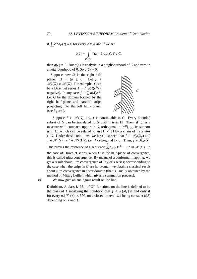
70 12. LEVINSON’S THEOREM Problem of Continuation
if∫
Ωeλzdµ(z) = 0 for everyλ ∈ Λ and if we set
g(ζ) =∫
K⊂Ω
f (z− ζ)dµ(z), ζ ∈ C,
theng(ζ) ≡ 0. Butg(ζ) is analytic in a neighbourhood ofC and zero ina neighbourhood of 0. Sog(ζ) ≡ 0.
Suppose nowΩ is the right halfplane. Ω = u ≥ 0. Let f ∈HΛ(Ω) ,H (Ω). For example,f canbe a Dirichlet seriesf =
∑
a(λ)eλz(λnegative). In any casef ∼ ∑
a(λ)eλz.Let G be the domain formed by theright half-plane and parallel stripsprojecting into the left half- plane.(see figure ).
Supposef ∈ H (G), i.e., f is continuable inG. Every boundedsubset ofG can be translated inG until it is in Ω. Then, if dµ is ameasure with compact support inG, orthogonal toeλzλ∈Λ, its supportis in Ωz which can be related to anΩo ⊂ Ω by a chain of translates⊂ G. Under these conditions, we have just seen thatf ∈ HΛ(Ωo) andf ∈H (G)⇒ f ∈HΛ(Ωζ), i.e., f orthogonal todµ. Then, f ∈HΛ(G).
This proves the existence of a sequenceN∑
oaN(λ)eλz → f in H (G). In
the case of Dirichlet series, whenΩ is the half-plane of convergence,this is called ultra convergence. By means of a conformal mapping, weget a result about ultra convergence of Taylor’s series; corresponding tothe case when the strips inG are horizontal, we obtain a classical resultabout ultra convergence in a star domain (that is usually obtained by themethod of Mittag Leffler, which gives a summation process).
We now give an analogous result on the line.73
Definition. A classKMn of C∞ functions on the line is defined to bethe class off satisfying the condition thatf ∈ KMn if and only iffor everyn, | f (n)(x)| < kMn on a closed intervalJ, k being constantk(J)depending onJ and f ;

2. Problem of continuation - Description of the problem 71
2. KMn is said to be quasi - analytic if the only function of theclass all of whose derivatives vanish at the origin is the zero function(see lecture 19, §1).
Suppose furtherf can be continued on the line in such a mannerthat f ∈ KMn. Then f is mean periodic with spectrumΛ. For letdµ be a measure with
∫
eiλxdµ(x) = 0 for everyλ ∈ Λ. Let g(ξ) =∫
If (x+ ξ)dµ(x), whereI is the support ofdµ. Now f ∈ KMn ⇒ g ∈
KMn. But g(n)(0) = 0 for all n. So g = 0. This means thatf andall its translates are orthogonal todµ, i.e.,τ( f ) , C . This gives that iff ∈ Cλ(I ) and f ∈ C (R), in order thatf ∈ CΛ(R) it is sufficient thatf ∈ KMn quasi - analytic. This kind of result was first given byS.Mandelbrojt (Mandelbrojt 1).@ These problems are considered in the lectures 13, 15 and 16 for thecomplex plane, and in the lectures 17 and 18 for the line. We give nowsome very easy results.


Lecture 13
A method of continuation
1 Principle of continuation
Give f ∈ HΛ(Ω), first we shall find out a method of continuation off 74
to a pointZ. Suppose that it is possible to find a measuredµ = dµZ withsupport inΩ such thatdµ−δz is orthogonal toeλz for everyλ ∈ Λ, whereδz is the Dirac measure atZ. In other words, the following relation isgiven
eλz=
∫ eλz
dµ(z). (1)
We can try to replaceeλz by f (z) in (1), i.e. we can try to get
f (Z) =∫
f (z)dµ(z). (2)
This is certainly possible whenZ ∈ Λ, since f ∈ HΛ(Ω). WhenZ < Ω this gives a means of definingf at Z. More precisely, iff can beapproximated by
∑
a(λ)eλz in Ω, then formally we have the followingrelations
f (Z) −∑
a(λ)eλZ=
∫
K[ f (z) −
∑
a(λ)eλz]dµZ(z);
| f (z) −∑
a(λ)eλz| < ε∫
|dµz|
Hence the majorization does not depend onZ but ondµz. If Z belongsto a continuumC and if it is possible to find a measuredµz with support
73

74 13. A method of continuation
in K ⊂ Ω,K independent ofZ, such that∫
|dµz| < B uniformly in Z,then f can be approximated onC by the same sums
∑
a(λ)eλz as onK and sup
Z∈C| f (Z)| ≤ Const max
z∈K| f (z)|. To find the measuredµ is exactly
the same thing as to find its Fourier transform. In other words, we seekan entire functionM(w) = MZ(w) of exponential type with conjugatediagram inΩ such that−M(w) + ewZ vanishes forw ∈ Λ
Moreover, we wantM(w) to be the typeM(w) =1
2πi
∫ ϕ(z)Z ewzdZ
C, C75
being a curve inΩ fixed for all Z, andϕZ(z) uniformly bounded onCwhenZ belongs to a given continuum. According to formulae (1) and(2) in lecture 9, this last condition is satisfied wheneverMZ(w) admits auniform majorization
|MZ(w)| < K
1+ r2erk(θ)(w = reiθ) (3)
andC is the frontier for the convex set defined by
X cosθ − ysinθ ≤ k(θ) (4)
Then, (2) can be written as
f (Z) =1
2πi
∫
CϕZ(z) f (z)dz (5)
Let us remark that (3) need not be required for everyθ; if C can bedefined from (4) withθ ∈ S,S being a given subset of [0,2n], it is suffi-cient to have (3) whenθεS, and to assume thatMZ(w) is of exponentialtype; in particular, ifC is a convex polygon,S can be taken as a discreteset; in this case, we shall say“S is associated with C”.
Thus the principle of continuation can be formulated as follows: LetD(w) be an entire function of exponential type, vanishingΛ, with itsconjugate diagramJ contained inΩ. Let C be a convex polygon con-tained inΩ, and containingJ in its interior, and letS be a set associatedwith C. LetZ ∈ G, and suppose that, for eachZ, there exists a meromor-
phic functionA(w) = AZ(w), with polar part∑
λ∈Λ
eλZ
D′(λ)(w− λ)uniformly

2. Application of the principle of continuation 75
bounded whenθ ∈ S, and also when|w| = Rj lim Rj = ∞. ThenC andMZ(w) = D(w)AZ(w) satisfy the condition above. If we put
ϕz(w) =
∞iα∫
0
D(w)AZ(w)e−wzdw (6)
and if f ∈HΛ(Ω), (5) defines a continuation off in G, in such a manner76
that 10) on G f is a uniform limit of the same Dirichlet polynomials∑
a(λ)eλz(λ ∈ Λ) as onC (in particular, ifG is an open set,f is analyticon G, if G is an open set andG ∩ Ω , φ, (5) provides an analyticcontinuation off fromΩ into G).
20) onG, | f (Z)| < K supZ,∈C| f (z)|,K independent ofZ. (7)
Let us remark that, ifΛ is the sequence of the negative integers, ourprinciple of continuation gives the same result as the Cauchy formula,translated after a change of variableζ = e−z. Thus, (5) is a kind ofgeneralization of the Cauchy formula.
2 Application of the principle of continuation
We have a solution of the problem of continuation of we can constructthe functionD(w) andA(w) satisfying the above principle. We shall ap-ply this principle directly in simple cases and with a little modificationin other cases, for example forCΛ(K),K ⊂ R; then we shall obtain,for certain real sequenceΛ, the analytic continuation off ∈ CΛ(K);this forms the main result in the thesis ofL. Schwartz (Schwartz 1 (seelecture 16)). In certain cases, we shall takeA(w) having an integral rep-
resentation of the formA(w) = limj→∞
∫
C j
ew′Zdw′
D(w′)(w− w′),C j being certain
closed curves (see lecture 15).We first apply this principle in the simplest way. We supposeΛ
is a negative sequence,viz. every element ofΛ is a negative numberΛ = λλ<0. The requiredD(w) is provided by the canonical productD(w) = C(w) =
∏
λ∈Λ(1 − w2
λ2 ). This begin achieved, to constructA(w),
76 13. A method of continuation
we make some more assumptions onΛ in such a way that the polarpart of A(w) is normally convergent outside the union of small circles77
Uλ = |w− λ| < ρ,A(w) being uniformly majorized outside these smallcircles.I. Let Λ possess a densityD.
We haveD(w) = C(w) =∏
(1 − w2
λ2 ) and the conjugate diagramof C(w) is the segment joiningiπD and−iπD. We takeΩ to be a smalldomain containing this segment so thatf is analytic inΩ. SupposeA(w)is of the form
A(w) =∑ eλZ
C′(λ)(w− λ)(1)
In order that this series is normally convergent whenZ = X + iYvaries outsideUλ =
∣
∣
∣w − λ∣
∣
∣ < ζ, it is sufficient to have exp(λX −log |C′(λ)|) < eλε or again the following relation
X > δ + ε, ε > 0, whereδ = lim suplog |C′(λ)|
λ.
Definition. WhenΛ possesses a densityD, δ = lim sup log |C′(λ)|λ
is de-fined as the“ index of condensation”of Λ.
A sequenceΛ is called “regular” if limλ′,λ
sup|λ′ − λ| > 0. If Λ is
a regular sequence it can be proved (V. Bernstein, note II) thatδ = 0.Whenδ = 0. we have the
Theorem.Let Λ be a negative sequence with density D and let f∈HΛ(Ω), Ω ⊃ [−iπD, iπD]. Whenδ = 0, every function f∈ HΛ(Ω) canbe continued analytically in the right half plane x≥ 0 into a sum ofconvergent Dirichlet’s series
∑
a(λ)eλz
As a consequence of this theorem we obtain a classical result onDirichlet’s series. Letf (z) =
∑
a(λ)eλz be a Dirichlet’s series whereΛis a sequence of positive number having∞ as the sole limit point. Iff (z)is convergent forReZ= xo, it is also convergent forReZ= x > xo. Thus78
one can define the abscissa of convergence,σa, as an ordinate throughx = σa to the right of which
∑
a(λ)eλz is convergent and to the left ofwhich
∑
a(λ)eλz is not convergentWe have the following corollary:

2. Application of the principle of continuation 77
Corollary. The Dirichlet’s series∑
a(λ)eλz with exponents extractedfrom a sequence having a density D and index of condensation zero,admits at least one singularity on every segment of length2πD on itsabscissa of convergence. If D= 0 and ifΛ is a sequence of integers, thechange of variablesζ = e−z gives the Fabry theorem, viz., the circle ofconvergence is the natural boundary of a gap series.
Proof of the Corollary. Indeed if there is nosingularity,Ω can be taken very narrow con-taining this segment and the Dirichlet’s seriesis ultra-convergent inΩ (lecture 12, 2). Tak-ing a segment of length 2πD in Ω parallel tothis segment and to the left of the abscissa ofconvergenceσ f we see by the above theoremthat the Dirichlet’s series is convergent to theleft of σ f , which is impossible.
Let σk (“abscissa of holomorphy”) be the in-fimum of theσ such thatf (z) =
∑
a(λ)eλz isanalytically continuable for Rez> σ. Whenδ , 0 and if σh andσc are the abscissa ofholomorphy and convergence of Dirichlet’sseries
∑
a(λ)eλz, applying as above the re-sult about ultra-convergence and the condi-tion that it converges forx > σh + δ + ε weobtain the following result of V. Bernstein.
Theorem.σc − σh ≤ δ, and every segment of length2πD on Re z= σh 79
contains at least one singularity.
Suppose nowf (z) is an entire function,f (z) =∑
λ∈Λa(λ)e−λz. The
inequality (7) allows us to compare the order of magnitude off in thewhole plane and in the strip, whenx = Rez→ −∞. LetY be a horizon-tal strip of width 2πD + ε,M(x) = sup
Rez=x| f (z)|

78 13. A method of continuation
MY (x) supRez=x,z∈Y
| f (z)|. We have immediately
Theorem. M(x) ≤ KMY (x − δ − ε′),K depending only onΛ, ε andε′(ε > 0, ε′ > 0 width ofY = 2πD + ε)
We obviously get the same result on supposingY to be a curvilinearstrip.II. Let the sequenceΛ possess a finite mean upper densityD.. If Λ isregular and
∣
∣
∣λ′ − λ∣
∣
∣ > h > 0, it has been proved by S. Mandelbrojt that
lim sup log |C′(λ)|λ
= δ < B, whereB = B(D.,h) is a constant dependingon D.. andh (Mandelbrojt 2, 3).
We know that the conjugate diagram ofC(w) is contained in a circleof radiusπD.. We supposeΩ to be a circular with radiusπD.
+ ε around0 and letf ∈ HΛ(Ω). We takeA(w) given by (1) as in the part.A(w) isnormally convergent whenX > δ + ε. Thus we have a continuation of80

2. Application of the principle of continuation 79
f into the half planeG to the right ofΩ at a distanceB(D.,h) from itscenter, and inG, f is represented by a convergent Dirichlet’s series. Theresult proved in the last lecture about the continuation by means of trans-lates ofΩ permits us to find again the following result of S. Mandelbrojt(Mandelbrojt 2,3) which generalizes a theorem of A. Ostrowski’s.
Theorem. If σc is the abscissa of convergence of f as a Dirichlet’s se-ries, then f cannot be analytically continued into the domain generatedby circular discsΩζ of radiusπD.
+ ε, ε > 0 whose centersζ belong toa continuumC which has at least one pointζ with Reζ > σ and at leastone pointζ′ ∈ C with Reζ′ < σc − B(D.,h).
Now, if we continuef with ζ running along a closed path, we comeback to the original function (see fig.), according to theorem 2, lecture9, §2.
It is natural to ask: Is it possible to have such a figure with singular-ities inside? In other words, can we have continuation off (Z) along a

80 13. A method of continuation
chain of translatesΩζ whose union forms an annular region with singu-larities of f (Z) in the interior of the bounding curves? We shall consider81
this question in a later lecture. (Lect. 16)By the same argument as inI , we get a result about the order of
magnitude off in the plane the whole plane and in a strip. HereY is ahorizontal strip, of width 2πD.
+ ε.
Theorem. M(x) ≥ KMY (X − B − ε′), K depending only onΛ, ε andε(ε > 0, ε′ > 0) widthY = 2πD.
+ ε)
Analogous result hold for curvilinear strips.

Lecture 14
Lemmas concerningminimum modulus ofcanonical products
We need certain lemmas to find minorization of∣
∣
∣C(w)∣
∣
∣ 82
Lemma 1. SupposeD. < ∞. Let C(w) =∏
(
1− w2
λ2
)
. Givenε >
0, there exists an infinity of Rj ր ∞ such that for|w| = Rj we have∣
∣
∣C(w)∣
∣
∣ > e−εRj .
Proof. We have∣
∣
∣
∣
∣
C(w)∣
∣
∣
∣
∣
≥∣
∣
∣
∣
∣
1− r2
|λ2|
∣
∣
∣
∣
∣
, where|w| = r. We apply Carleman’s
formula to the functionC∗(w) =∏
(
1− w2
|λ2|
)
, in the upper half plane
v ≥ 0. Then we have the following relation:
∫ R
−Rlog
∣
∣
∣C∗(u)∣
∣
∣
du
u2= o (1)
This relation implies that there exists an infinity ofRj ր ∞ such thatlog
∣
∣
∣C∗(Rj)∣
∣
∣ > −εRj ; i.e for |w| = Rj |C(w)| ≥ |C∗(Rj)| > e−εRj .
Lemma 2 (H. Cartan). Supposeδ > 0 and M1, . . . ,Mn are n givenpoints in the complex plane. Then we can find m discs, m≤ n the sum of
81

82 14. Lemmas concerning minimum modulus of...
whose radii is2nδ in such a manner that if M is any point outside these
discs the product of the distances MM1, . . . ,MMn >
(nδe
)n
.
Proof. Let k1 be the largest integer such that there exists a disc of radiusk1δ containing at leastk1 of the pointsM j , and letC1 be such a disc.ObviouslyC1 contains exactlyk1 points M j . Let us remove thesek1
points, and define in the same manner from the remaining points (ifthere exist any ) a discC2 of radiuskδ2, and so on: we get a finite numberof discs, sayC1, . . . ,Cm, of radiik1δ, . . . , kmδ, andk1+· · ·+km = n. Now,83
let Γ1, . . . ,Γm be discs concentric withC1 . . .Cm and of twice the radii.From the construction ofC1, . . . ,Cm, it follows that, if a disc
∫
(M, kδ)of centerM and radiuskδ contains at leastk pointsM j , then it containsa pointMq ∈ Cq with kq ≥ k; thusM ∈ Γq.
Suppose nowM < ∪Γ j ; then, ever∫
(M, kδ) contains at mostk − 1pointsM j . Let the distancesMM j be thatMM1 ≤ MM2 · · ·MMn. ThenMM1 > δ,MM2 > 2δ, . . . ,MMn > nδ, and
MM1 · MM2 · · ·MMn > n!δn >
(nδe
)n
that completes the proof.Definitions. Given a finite set of pointsM j andδ > 0, we callΓ j asystem of “Cartan discs relative toM j andδ”.
Let Λ be a sequence of points in the complex plane without finitepoints of accumulation, andδ > 0. By a system of “Cartan discs relativeto Λ and δ”, we shall mean the union of the system of Cartan discsrelative toΛ and the annulus 2n − 1 ≤ |z| < 2n+1 − 1(n = 0,1, . . . , )
Lemma 3. Suppose the symmetrical sequenceΛ has a density D. Givenε > 0 andδ > 0 we have|C(w)| = ∏ |1 − w2/λ2| > e−ε|w| for |w| suffi-ciently large, and w varying outside Cartan discs of a system relative toΛ andδ.
Proof. Write C(w) =∏
1
∏
2where
∏
1=
∏
r/γ<|λ|<γr
(1 − w2/λ2), γ > 1 to
be chosen later to be near 1. Denoting byn(r) the distribution function

83
of |λ|, we have the following relations:
log |∏
2
| >
r/γ∫
o
+
∫ ∞
rγ
[
log∣
∣
∣1− r2
λ2
∣
∣
∣dn(λ)
]
(r = |w|)
= n
(
rγ
)
log(γ2 − 1)− n(γr) log
(
1− 1γ2
)
+ r∫ 1/γ
0
21− u2
D(ru)du−∫ ∞
γ
2u2 − 1
D(ru)du
1/γ∫
o
2u2 − 1
D(ru)du< logγ + 1γ − 1
(D + 0(1)) (r → ∞)
and∫ ∞
γ
2u2 − 1
D(ru)du< logγ + 1γ − 1
(D + 0(1)) (r → ∞)
n
(
rγ
)
log(γ2 − 1)− n(γr) log
(
1− 1γ2
)
> 2 logγ.n(γr) > 0
if γ2 < 2. Then log∣
∣
∣
∏
2
∣
∣
∣ > −ε/2 if γ2 < 2, andr large enough. Now 84∏
1 is a product ofN terms,N < 2Dr (γ − 1/γ), if r is large enough.Let
∏
1,n be the product of those terms, whose zeros are in use in theannulus 2n − 1 ≤ |z| ≤ 2n+1 − 1;
∏
1 can be written as∏
1,n .∏
1,n+1 for aconvenientn. Takew outside any Cartan disc and suppose (if necessary,by changing the sign ofλ) |w− λ| ≤ |w+ λ|; then
∣
∣
∣
∏
1,n
∣
∣
∣ >∏
1,n
∣
∣
∣1− wλ
∣
∣
∣ >1
(γr)M
∏
1,n
∣
∣
∣w− λ∣
∣
∣ >1
(γr)M
(Mδ
e
)
M
whereM is the number of terms of∏
1,n; M ≤ N < 2Dr(γ − 1γ
)
log∣
∣
∣
∏
1,n
∣
∣
∣ > M logmγer= r
Mr
(
Mr.δ
γe
)
> −ε4
r,
if γ is chosen near enough to 1. That completes the proof.

84 14. Lemmas concerning minimum modulus of...
Lemma 4. Suppose∑ 1λ< ∞ and C(w) =
∏
(1− w2
λ2). For almost all
θ, we havelimr→∞
log|C(reiθ)|
r= 0.
Proof. We choose the set of “ Cartan discs”,Γ, as in the previous lemma.Let θΓ be the angle which a circleΓ subtends at origin. Since the radiusof the circleΓ are of the from 2nδ with preciselyn pointsλ in sideΓ, we
haveθΓ ∼∑
λ∈Γ
1|λ| and
∑ |θΓ| < ∞
0
If we consider only those circles far away from the origin, we have85∑ |θΓ| < ε. Then outside of these anglesθ, by the previous lemma,
we have|C(w)| > e−ε|w|. Thus we have limlog |C(w)|
r=0 almost every-
where.One can prove, in the same manner, the following lemma.
Lemma 5. If D = 0, thenlimlog |C(w)|
r= 0, when w→ ∞, w vary ing
outside of Cartan discs associated withΛ.
Lemma 6. Let Φ(w) and ψ(w) be two functions of exponential type.Suppose|Φ(w)| < |ψ(w)| < e|v| outside of discsΓ, each of which is ofradius 2kε(k = k(Γ): an integer) and contains k zeros ofψ. Then, forsufficiently smallε, |Φ(w)| < e|v|.
Proof. Let w belong to the frontier of aΓ. Applying Jensen’s formulato ψ on a circleC of centerw and radiusr, we get
log |ψ(w)| < 12π
∫ 2π
0log |ψ(w) + reiθ|dθ − log
rk
(2kε)k
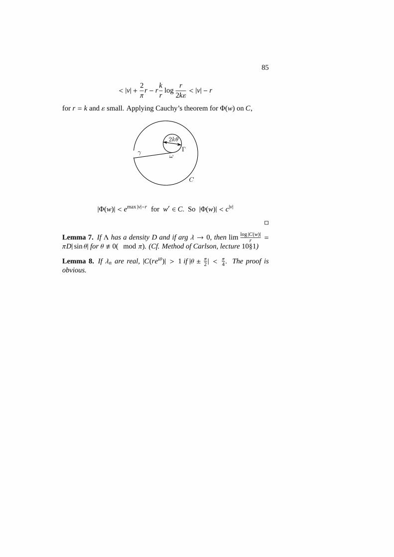
85
< |v| + 2π
r − rkr
logr
2kε< |v| − r
for r = k andε small. Applying Cauchy’s theorem forΦ(w) onC,
|Φ(w)| < emax|v|−r for w′ ∈ C. So |Φ(w)| < c|v|
Lemma 7. If Λ has a density D and if argλ → 0, thenlim log |C(w)|r =
πD| sinθ| for θ . 0( modπ). (Cf. Method of Carlson, lecture10§1)
Lemma 8. If λn are real, |C(reiθ)| > 1 if |θ ± π2 | <
π4. The proof is
obvious.


Lecture 15
Continuation Theorems
1 Theorems about negative sequences, or sequencescontained in a salient angle
In Lecture 13, we have seen how the principle of continuation can be86
applied when the sequenceΛ consists of only negative numbers. We
had to suppose that the canonical productC(w) =∏
(1 − w2
λ2)(λ ∈ Λ)
satisfies the condition that| logC′(λ)|
λis bounded, and thatΛ possesses
a density or, at least, a, mean upper density. Then, for a convenientΩ,each f ∈ HΛ(Ω) can be “continued” in a certain half-planex > xo. Itis not a true continuation whenΩ and the half plane have no commonpoints. Is it possible to consider the function, defined in the half plane,as an analytic continuation off ? This question will be solved by the useof result about minimum moduls ofC(w), and a representation ofAz(w)as a contour integral.
Suppose we fix argZ to satisfy the condition that|argZ| < π
2−α, α >
0. Consider the contourC, formed of the lines [r ei(π−α), r ei(π+α),0≤ r ≤ R] and the circular are [Rei(π+θ)|θ| ≤ α], and taken in the posi-tive direction. Letw be outside the angle made by this contourC. ByCauchy’s formula, we have the following equation:
87
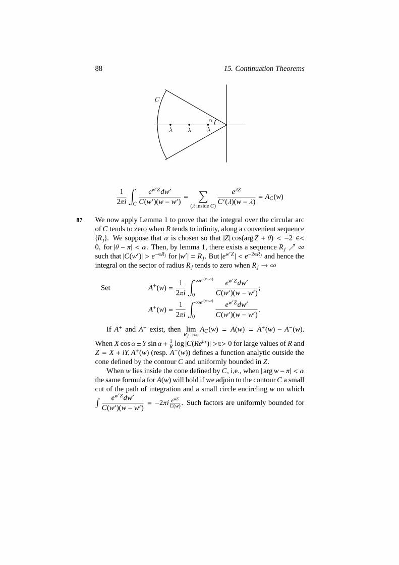
88 15. Continuation Theorems
12πi
∫
C
ew′Zdw′
C(w′)(w− w′)=
∑
(λ insideC)
eλZ
C′(λ)(w− λ)= AC(w)
We now apply Lemma 1 to prove that the integral over the circular arc87
of C tends to zero whenR tends to infinity, along a convenient sequenceRj. We suppose thatα is chosen so that|Z| cos(argZ + θ) < −2 ∈<0, for |θ − π| < α. Then, by lemma 1, there exists a sequenceRj ր ∞such that|C(w′)| > e−∈Rj for |w′| = Rj . But |ew′Z| < e−2∈Rj and hence theintegral on the sector of radiusRj tends to zero whenRj → ∞
Set A+(w) =1
2πi
∫ ∞ei(π−α)
0
ew′Zdw′
C(w′)(w− w′);
A+(w) =1
2πi
∫ ∞ei(π+α)
0
ew′Zdw′
C(w′)(w− w′).
If A+ and A− exist, then limRj→∞
AC(w) = A(w) = A+(w) − A−(w).
WhenX cosα±Ysinα+ 1R log |C(Reiα)| >∈> 0 for large values ofRand
Z = X + iY,A+(w) (resp.A−(w)) defines a function analytic outside thecone defined by the contourC and uniformly bounded inZ.
Whenw lies inside the cone defined byC, i,e., when|argw− π| < αthe same formula forA(w) will hold if we adjoin to the contourC a smallcut of the path of integration and a small circle encirclingw on which∫ ew′Zdw′
C(w′)(w− w′)= −2πi ewZ
C(w) . Such factors are uniformly bounded for

1. Theorems about negative sequences,... 89
|w| = Rj , |argw− π| < α. Thus we haveA(w) satisfying our requirementof lecture 13; §1) it is uniformly bounded inZ whenw varies outside thecone generated byC or when|w| = Rj , |argw − π| < α; 2) it has polarpart
∑
λeλz/C′(λ)(w− λ), and 3) it is analytic everywhere except at these
poles) whereverZ satisfies the following conditions:
a) for a sequence of values ofRj ր ∞, and for|θ − π| ≤ α we have|Z| 88
cos(argZ + θ) − 1Rj
log |C(Rjeiθ)| < − ∈< 0;
b) for large values ofR, we have
X cosα ± Ysinα +1R
log |C(Rei(π±α))| >∈> 0, (Z = X + iY).
We will be able to find the variability ofZ satisfying these conditionsby making some more assumptions onΛ.
1. Λ possesses a densityBy the lemma of Carlson, ifθ . 0( modπ), we havelim log |C(Reiθ)|
R =
πD| sinθ|. Using this and lemma 3, we are led to consider only condi-tion a) to determine the variability ofZ. Moreover, by the continuationdeveloped in Lecture 13 for negative sequence we have the followingtheorem:
Theorem.SupposeΛ is a sequence of negative numbers having a den-sity D andΩ an open set containing the segment(−iπD, iπD). Then itis possible to continue every function f∈ HΛ(Ω) to be analytic in the
right half-plane x≥ 0. Moreover for|argZ| < β <π
2the continuation
yields us a function which is bounded and uniformly approximated bylinear combination of eλz, λ ∈ Λ. If Λ has a finite index of condensationδ, the continuation yields us a Dirichlet’s series convergent for x≥ δ
The same statement holds for a sequenceΛ without density, if wereplaceD by Dmax. For there existsΛ′ ⊃ Λ,Λ′ having a density, anddensityΛ′ = DmaxΛ (see Appendix 1)
Corollary. The sum of a Dirichlet’s series whose sequence of exponentspossesses a maximum density Dmax, admits at least one singularity on

90 15. Continuation Theorems
every segment of length larger then2πDmax on its abscissa of holomor-phy.
2. Λ has a finite mean upper densityD.
In this case, by lemma 8,|C(reiθ)| > 1 for |θ ± pi2| < π
4. So, we89
are obliged to take into consideration both the conditions a) and b) todetermine the variability ofZ. As before the continuation developed forthis case in Lecture 13, gives us a similar theorem for continuation off ∈ HΛ(Ω), whereΩ is an open set the containing the circle|z| ≤ πD.,into that portion of the right half plane contained between the linesθ =
±π4
. The index of condensationδ is replaced by the constantB.
3. Λ is contained in a salient angleSupposeΛ is a sequence contained in a salient angular region around
the negative real axis, i.e.,Λ consists of pointsλ of the formrei(π+θ), |θ| ≤
β. Then using|C(w)| < (1 +|w|2|λ|2
) and |C(u)| < ∏ |1 − u2e2iβ
|λ|2∣
∣
∣ for
locating the conjugate diagram and using|C(w)| > ∏ |1 − w2e2iβ
|λ2|2iβ
∣
∣
∣ If
π
2< argw < π − β for having the minorization of|C(w)| we can prove
similar theorems takingα > β
Case 1 Case 2 Case 3
2 Theorems for symmetric sequences
First letΛ be a real symmetric sequence having a densityD. The canon-90

2. Theorems for symmetric sequences 91
ical productC(w) =∏
λ∈Λ(1− w2
λ2) has for its conjugate diagram the seg-
ment (−iπD, iπDλ)∈Λ. LetΩ be a domain containing this segment. Theconjugate diagrams ofC(w)ewc andC(w)e−wc, c > 0, are two segmentsparallel to the given segment and on either side of it.
For sufficiently smallc > 0, they are contained inΩ. Now we takeD(w) = C(w)Ch(cw)[2Ch(cw) = ewc
+ e−wc] in order that we get asimultaneous majorization ofew′Z/D(w′) (w − w′) on two circular arcsof the contour of integration situated symmetrically.
We take the contourC consisting of the linesreiα andre−iα,−R ≤r ≤ R and circular arcsReiθ and−Reiθ,−α ≤ θ ≤ α. Let w be a pointwith
∣
∣
∣w − w′∣
∣
∣ > 1 for any pointw′ in the interior of this contour. ByCauchy’s theorem we have
AC(w) =1
2πi
∫
C
ew′Zdw′
D(w′)(w− w′)=
∑
λinsideC
eλZ/D′(λ)(w− λ).
Now, by Lemma 1, we have∣
∣
∣C(w)∣
∣
∣ > e−∈Rj on an infinity of circlesof radii 1Rj ր ∞ and so taking into account the majorization
∣
∣
∣ew′z/D(w′)∣
∣
∣ < er(R∣
∣
∣ cos(ϕ+θ)∣
∣
∣+∈−C∣
∣
∣ cosθ∣
∣
∣)
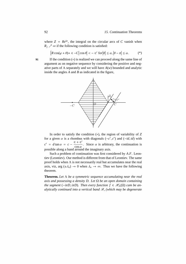
92 15. Continuation Theorems
whereZ = Reiϕ, the integral on the circular arcs ofC vanish whenRj ր ∞ if the following condition is satisfied:
Rcos(ϕ + θ)+ ∈ −C∣
∣
∣ cosθ∣
∣
∣ < − ∈′ for∣
∣
∣θ∣
∣
∣ ≤ α,∣
∣
∣θ − π∣
∣
∣ ≤ α. (*)
If the condition (∗) is realized we can proceed along the same line of91
argument as on negative sequence by considering the positive and neg-ative parts ofΛ separately and we will haveA(w) bounded and analyticinside the anglesA andB as indicated in the figure,
In order to satisfy the condition (∗), the region of variability ofZfor a givenα is a rhombus with diagonals (−c′, c′) and (−id, id) with
c′ = d tanα = c − ∈ + ∈′
cosα. Sinceα is arbitrary, the continuation is
possible along a band around the imaginary axis.Such a problem of continuation was first considered byA.F. Leon-
tiev (Leontiev). Our method is different from that of Leontiev. The sameproof holds whenΛ is not necessarily real but accumulates near the realaxis, viz, arg (±λn) → 0 whenλn → ∞. Thus we have the followingtheorem.
Theorem.LetΛ be a symmetric sequence accumulating near the realaxis and possessing a density D. LetΩ be an open domain containingthe segment(−iπD, iπD). Then every function f∈ HΛ(Ω) cam be an-alytically continued into a vertical bandB, (which may be degenerate

2. Theorems for symmetric sequences 93
into a half-plane or the whole plane) such that on each segment of lengthlarger than2πD on the boundary ofB there is at least one singularityof the function.
The last part of the theorem results from the relationf ∈HΛ(Ωζ) for 92
every translateΩζ ofΩ, such thatf is analytic along a chain of translatesjoiningΩζ toΩ (Lecture 12, §2). Moreover, one can provef ∈HΩ(B)(Kahane 1, p. 98).
Suppose now thatΛ is a symmetric sequence accumulating near thereal axis and having a mean upper densityD.. The above method can
be applied, if we takeα >π
2, by using lemma 8 instead of lemma 7,
Lecture 14. This leads to the following result.
Theorem.SupposeΛ is symmetric, accumulates near the real axis, andpossesses a mean upper densityD.t. Take asΩ an open set containingthe disc|z| ≤ πD., and letΩc andΩ−c be its translates by c and−c,∣
∣
∣ argc∣
∣
∣ <π
4. Then every f∈ HΛ(Ωc ∪ Ω−c) can be continued in a
rectangle whose sides make anglesπ
4(mod
π
2) with the real axis, and
having c and−c as vertices.


Lecture 16
Further Theorems ofContinuation
1 Theorem of Schwartz
We have proved in Lecture 11, §4 that ifΛ is a negative sequence,Λ = 93 − λn
and∑ 1λn= ∞, thenCΛ(I ) = C (I ). Conversely if
∑ 1λn
< ∞,
thenCΛ(I ) , C (I ). Let us recall that the function
D(w) =N
∏
1
(
1+wλn
) ∞∏
N+1
sinπw/λn
w/λn
satisfiesD(Λ) = 0,D(u) = 0(1u2
) and∣
∣
∣D(w)∣
∣
∣ < Keh|v|, whereh =
π∞∑
N+1
1λn
.
Supposef ∈ CΛ(I ),Λ = −λn and∑ 1λn
< ∞. Then we shall prove
that f can be continued to a half-plane at the right, above and belowI .We takeI = (−h,h) andAZ(w) =
∑
e−λZ/D′(λ)(w−λ), whereD(λ) =0. The idea is still to defineAZ(w) as an integral. To do this, we take aset of “Cartan circles”Γ constructed for a given∈> 0 andΛ (see Lecture14). Letw lie on a circleΓ1 concentric to circleΓ and of radius equal to
95

96 16. Further Theorems of Continuation
∈ + radius ofΓ. Consider the following expression:
AZ(w) =1
2πi
∫
ew′Zdw′
D(w′)(w− w′),wε oneΓ1
We have∣
∣
∣ew′Z∣
∣
∣ = erRcos(ϕ+θ),Z = Reiϕ,w′ = reiθ.
2. Interpolation Results 97
When Z varies in an angle∣
∣
∣ arg(Z− ∈′)∣
∣
∣ <<π
2(∈′> 0), one can
choose∈′ − and then theΓ′s so thatAZ(w) is uniformly bounded inZ on ∪Γ1. Indeed if the “Cartan circles”Γ are contained in an angle94∣
∣
∣ argw − π
2
∣
∣
∣ < α and if∣
∣
∣ arg(Z− ∈′)∣
∣
∣ ≤ π/2 − α we have a uniform
majorization. Also by construction,α → 0 when∈→ 0. Considerw2MZ(w) = AZ(w)D(w)w2. Outside the circlesΓ1 we have
∣
∣
∣w2MZ(w)∣
∣
∣ <
K1
∣
∣
∣w2D(w)∣
∣
∣. If ∈ is small enough, it follows, by lemma 6, lecture 14,that
∣
∣
∣w2MZ(w)∣
∣
∣ < K2eh|v| and also∣
∣
∣MZ(w)∣
∣
∣ < K2eh|v| uniformly in Z.Thus MZ(w) = Az(w)D(w) is the Fourier transform of a measure with
support in (−h,h). This enables us to definef (Z) =∫ h
−hf (z)dµZ(z).
Moreover,∫ ∣
∣
∣dµZ
∣
∣
∣ is bounded when∣
∣
∣ arg(Z− ∈′)∣
∣
∣ ≤ π
2− α. So f (Z) is
uniformly approximated in this angle by the same linear combinationsof e−λnZ which approximatef uniformly on (−h,h).
Theorem. If Λ is an imaginary sequence
iλn
such thatλn > 0,∑ 1λn
<
∞ every f ∈ CΛ(I ) is an analytic function, continuable into each righthalf - plane Rez≥ xo, xo in the interior of I. In each angle,
∣
∣
∣ arg(z−xo)∣
∣
∣ <
β <π
2(xo in the interior of I),
∣
∣
∣ f (z)∣
∣
∣ < K supx∈I
∣
∣
∣ f (x)∣
∣
∣,K depending only on
the angle.
Problem. It would be interesting to have a half-planeRez≤ xo insteadof the angle, in the last statement. This is certainly possible whenΛ isregular enough. Then, for a mean-periodic functionf of spectrumΛ wewould have
∣
∣
∣M(x)∣
∣
∣ = supRez=x
∣
∣
∣ f (z)∣
∣
∣ = K sup|ξ|<η
∣
∣
∣ f (x+ ξ)∣
∣
∣
a relation between the order of magnitude on the whole plane and on theline.
2 Interpolation Results
Supposef ∈HΛ(Ωc∪Ω−c). We have seen that ifΛ is real and with finite 95
D.,Ωc andΩ−c being circles with centres−c andc and radii larger than
98 16. Further Theorems of Continuation
πD., we can continuef into a rectangle with vertices atc and−c.Resultsof this type will give us some indications about the domain of existenceof the continued function.
SupposeD(w) is an entire function of exponential type withD(Λ) =0 and letΩ be an open set containing the conjugate diagram ofD. Wetake two translatesΩc andΩ−c of Ω. We try to construct a measuredν = dνc,Z(z) with support inΩ−c ∪ Ωc with the aid of the measureµsuch that we haveeλZ
=
∫
eλzdν wheneverλ ∈ Λ. Then we can definef (Z) =
∫
f (z)dνc,Z(z). We takedν = dµZ ∗ (δc − δ−c), whereδ is theDirac measure.C (dν) = M(w)(e−wc) = 2M(w)S h(cw). If we wantthe conjugate diagram ofM(w) in Ω we should expectM(w) to havethe same majorization asD(w). Let M(w) = D(w)A(w). We supposefirst thatD(w) andS h(cw) have no common zeros. We constructA(w)bounded in circles of radiusRj and on certain directions argw = θ ∈ E.Moreover, we want 2D(λ)S h(cλ)A(λ) = eλZ for eachλ ∈ Λ. For that wetake the following form ofA(w):
A(w) =ewZ
D(w)S h(cw)−∞∑
−∞
eµnZ
D(µn)S h′(µnc)(w− µn), µn =
iπnc.
Let E be the set of points in [0,2π] where limr→∞
inflog
∣
∣
∣D(reiθ)∣
∣
∣
r>∈> 0.
In order to have the conjugate diagram ofM(w) in Ω, it is sufficientto haveE dense in [0,2π], arg(i/c) ∈ E andZ ∈ [−c, c].
Here we give some results without details where this method is ap-96
plicable.
Theorem.Let C(w) be an entire function of exponential type withC(Λ) = 0 and the conjugate diagram of C(w) contained inΩ. Let the
set E(∈) of pointsθ for which limr→∞
inflog
∣
∣
∣C(reiθ)∣
∣
∣
r> − ∈ be dense in
(0,2π) for every∈> 0. Then every function f∈ HΛ(Ω−c ∪ Ωc) can becontinued analytically along the segment(−c, c).
We takeD(w) = C(w) sin(∈ w)S h(∈ w) and apply the above method.As a corollary, we get the following result: ifG =
⋃
ζ∈yΩζ and if
f ∈HΛ(G), f is analytically continuable in the convex closure ofY .

3. Theorems of Leontiev 99
A more interesting result is the following, which is more difficult toprove.
Theorem.SupposeΛ andΩ satisfy the hypothesis of the last theorem.Let Y be a connected set containing0, and G =
⋃
ζ∈Y Ωζ . If f ∈HΛ(Ω) and f ∈ H (G), f is analytically continuable in the convexclosure ofY .
From this theorem one can deduce that every analytic mean-periodicfunction on the line is analytically continuable in a horizontal strip (per-haps degenerated into a half-plane or the whole plane), such that everysegment of lengthL (mean period related toΛ) on the frontier of thestrip, contains at least one singularity off .
For the proofs, see (Kahane 1, p. 100-104).
3 Theorems of Leontiev
In (Leontiev) a method is given for the answer to the problem raised in97
lecture 13, viz. whether continuation along a chain of translatesΩζ ofΩ, with ζ in a closed curveY containing 0, of a functionf ∈ HΛ(Ω),implies that f is analytically continuable in the interior ofY . The an-swer is affirmative whenΩ is conveniently related toΛ. We sketch themethod of Leontiev.

100 16. Further Theorems of Continuation
Let C(w) =∞∏
1
(
1− w2
λ2n
)
= C (dα) and let
Ck(w) =∞∏
n=k
(
1− w
λ2n
)
= C (dαk).
HeuristicallyCk(w)→ 1 whenk→ ∞ anddαk → Dirac measure.More precisely,
∣
∣
∣Ck(w)∣
∣
∣ < Keπ|w|(D.+∈) and Ck(w) → 1 on every
compact set. Then, ifΓ is a curve around the disc|z| < π(D.+ ∈) the
Laplace-Borel transform ofCk(w), denoted byϕk(z), tends uniformly on
Γ to1z. SupposeΩ ⊃ Γ, and f ∈ HΛ(Ω); then the Dirichlet polynomial
fk(z) =1
2πi
∫
Γf (z+ ζ)ϕk(ζ)dζ tends uniformly tof (z) when
∣
∣
∣z∣
∣
∣ is small
enough.If we suppose alsof ∈ H (G),G =
⋃
ζ∈YΩζ , then fk(z) is defined by
the same formula in a neighbourhood ofY , so it is bounded and tendsuniformly to f (z) onY . Hence
Theorem.SupposeΛ is a symmetrical sequence ± λn
such that∣
∣
∣λn
∣
∣
∣
98
has a mean upper densityD., Ω is an open set containing|z| ≤ πD.,Y
is a closed curve passing through0, G =⋃
ζ∈YΩζ , and H is the interior
of Y . Then, every f∈ HΛ(Ω) which is analytically continuable in Gcan be continued in H as a function∈HΛ(H).
Corollary. Ifnλn→ 0, the domain of existence of every f∈ HΛ(H) is
simply-connected.
One can prove more, viz. the following result of Leontiev (statedpartly byG. Polya);
Theorem. Ifnλn→ 0, the domain of existence of every f∈ HΛ(Ω) is
convex.
For the proof, see (Leontiev).

Lecture 17
Continuation on the line
1 Some definitions about positive sequences
λn
=
Λ
We give a few definitions with notations. We have already defined (lec-99
ture 10)n(r)D(r),D.,D., D(r), D., D.. We define the following expres-sions to make list complete.
D(r) =1
log r
∫ r
o
dn(t)t
; D. = lim supr
D(r); D. = lim infr
D(r).
Takingλnր we shall consider lim sup(λn+1−λn) and lim inf(λn+1−λn).
The maximum densityDmax (minimum densityDmin) is the lowerbound (upper bound) of densities of sequences containing (containedin)and having a density. They are given by the following formulas (the firstone is proved in appendix 1; the second one follows from the remark atthe end.
Dmax = limζ→1−0
lim supr→∞
n(r) − n(ξr)r − ξr
Dmin = limζ→1−0
limr→∞
infn(r) − n(ξr
r − ξrWe call a sequenceregular if lim inf( λn+1− λn) > 0, and a sequence
with densityD well distributedif λn − nD = 0(1). (In general, we haveonly λn − nD = o(n)).
101
102 17. Continuation on the line
We define theupper distribution density. (lower distribution den-sity .) to be the lower bound (upper bound) of densities of well dis-tributed sequences containing (contained in)Λ. We have the followingformulae to calculate them:
. = limh→∞
limr→∞
supn(r + h) − n(r)
h
. = limh→∞
limr→∞
infn(r + h) − n(r)
h
Proof (for .): seth = limr→∞
supn(r + h) − n(r)
h. For sufficiently small100
∈> 0 there exists a well distributed sequenceΛ∗ ⊃ Λ and having adensityDh+ ∈. Therefore. ≤ lim inf
h→∞h. On the other hand, ifΛ∗ has a
densityD∗, we haven∗(r + h) − n∗(r) = hD∗ + 0(1) andD∗ > h − o(1).So. ≥ lim sup
h→∞h. Therefore∗ = lim
h→∞h.
Now . < ∞ means that for an arbitrary given interval of lengthh,there are only a bounded number ofλn in it. . < ∞ implies that thesequence is relatively dense in the sense of Bohr, i.e. there exists a welldistributed sequence contained in it. We have the following relationsbetween these densities:
1lim sup(λn+1 − λn)
≤ . ≤ Dmin ≤ D. ≤ D. ≤ D. ≤ D. ≤ ˆD. ≤ D.
D. ≤ Dmax ≤ . ≤1
lim inf(λn+1 − λn)
One can prove D. ≤ eD.(Mandelbrojt2, p.53).
If D.= D.,D. = D. and soDmin = Dmax.
If Λ1 + Λ2 = Λ,Λ having a density,D(Λ) = DmaxΛ1 ∗ DminΛ2.The definitions of well-distributed sequences, upper and lower dis-
tribution densities can be immediately translated in case of real non-symmetric sequences. We shall make use of these notions in the nextparagraph.
2 A problem of continuation on the line
SupposeΛ to be real, and take the spaceEΛ(I ). We are interested in101
2. A problem of continuation on the line 103
finding conditions onΛ andI in order that everyf ∈ EΛ(I ) is a restric-tion of an f ∈ EΛ. Moreover, if on I f belongs to a specified classof C∞-functions, we are interested to know the related properties of itscontinuation on the line.
It can be natural to expect that if∣
∣
∣I∣
∣
∣ > 2πDmax and if f ∈ CΛ(I ), thenf has a continuation so thatf ∈ CΛ. We shall give an example at the endof this lecture which shows that this is not true even whenf ∈ EΛ(I ).
SupposeΛ is a real regular sequence and let∣
∣
∣I∣
∣
∣ > 2π.. Can everyC∞-function∈ CΛ(I ) be continued into aC∞ - function inCΛ?
Definition. The classCI
Mn
for a given sequence
Mn
and a giveninterval I is defined to be the set ofC∞- functions onI which verifythe conditions
∣
∣
∣ f (n)∣
∣
∣ < KMn whereK depends only onf . We defineC
Mn
= C(−∞,∞)
Mn
.
Theorem.Suppose f∈ CΛ(I ) ∩ CI
Mn
, Λ real and regular, Mn ր|I | > 2π.. Then f can be continued into a function belonging toCΛ ∩C
Mn+p
for an integer p= p(Λ, I ).
It is sufficient to prove theorem for well distributed sequences, sincewe can findaΛ′ ⊃ Λ with |I | > 2π.. We supposeI to be symmetricwith respect to the origin.
Consider the canonical product
C(w) = (w− λo)∞∏
n=1
(
1− wλn
) (
1− wλn
)
we use the following result ofB. Levin aboutC(w). (Levin 1 and 2; 102
Mandelbrojt 3).C(w) is of typeΠ, |C(u)| < K(1+ |u|N), and∣
∣
∣C′(λn)∣
∣
∣ >
K′/(1+ |λn|N) whereK,K′ andN are dependent on the given sequence.C(w) is not the transform of a measure but of a distribution. We want
to construct a distribution whose transformM(w) has the same type asC(w) and satisfies the equationM(w) − eiwX
= 0 wheneverW ∈ Λ.In order to constructM(w), we takeM(w) = C(w)A(w),A(w) having apolar part≈ ∑
e(iλnX)/C′(λn) (w− λn)
. To assure normal convergence
we takeM(w) = wqC(w)∑
n
eiλnX
λqnC′(λn)(w− λn)
. This series is normally

104 17. Continuation on the line
convergent outside circles of radius∈ around theλ′ns for q > N + 2. Wewant to have a uniform majorization forMX(w). For this take a striparound the real axis: in this strip we have (Phragmen Lindelof
∣
∣
∣C(w)∣
∣
∣ <
K′|1+w|N; then in the strip minus these circles∣
∣
∣Mx(w)∣
∣
∣ < K′′∣
∣
∣w∣
∣
∣
q∣∣
∣1+w∣
∣
∣
N
and (Cauchy)∣
∣
∣MX(u)∣
∣
∣ <K′′
1+ u2(1+ up) for p even,p ≥ N+ q+ 2. Thus
MX(u) = C (TX),Tx = dµx +dp
dxpdvx has support inI , and∫
I
∣
∣
∣dµx
∣
∣
∣ and∫
I
∣
∣
∣dvx
∣
∣
∣ are uniformly bounded.Let us considerf ∈ EI (Λ) ; we can continuef at the pointx by the
formula
f (X) = 〈 f j ,Tx〉 =∫
I( f dµx + f (p)dvx).
By our standard argument, the continued function belongs toEΛ.More over, if Mn ր and f ∈ CI Mn, then the continued function∈C
Mn+p
.For a refinement of this result, see (Kahane 2).In this type of result. is the good density to consider. Actually103
we cannot get more if we replace. by Dmax. In order to show this weconstruct an example ofΛ and f ∈ CΛ(I ), f a C∞- function such thatf < CΛ andΛ has. = 1 andD. = Dmax = 0.
We takeΛ to be a sequence of integers which are situated in sucha manner that 2n of them are in an intervalIn, the intervalsIn beingdisjoint and having lengths which increase indefinitely. To do this wetake pn = nk, k > 1 and the sequenceΛ is the union of the sets
pn −n, pn − (n− 1), . . . , pn + n
. It is verified easily thatD = 0 and. = 1.We shall construct a functionf ∈ CΛ(I ), I = [−π + ε, π− ∈] and notcontinuable inEΛ, nor even inD ′
Λ.
Let α(x) =∞∑
−∞C jei jx . We can chooseC j in such a manner that
Co = 1 andα(x) vanishes onI . By the theorem of Denjoy Carlemanwe can haveα(x) to be not in any quasi-analytic class (lecture 19, §2),but in the classC
nαn for α > 1. Then∣
∣
∣α(k)(x)∣
∣
∣ < kαk. As α(k)(x) =
(i)k ∑
C j jkei jx je,∣
∣
∣C j
∣
∣
∣ <|α(k)|
jK. Hence
∣
∣
∣C j
∣
∣
∣ < minn
nαn
| j|n < e− jα , α′ < 1.

2. A problem of continuation on the line 105
Also∑
| j|≥n|C j | < e−nβ , β < 1. This majorizesSn(x) =
n∑
−nC jei jx on I . Let
f (x) =∞∑
n=1aneipnxSn(x). If
∑ |an|e−nβ < ∞, f is continuous onI . We
can takean such that∑
anpmn e−nβ < ∞ for everym andan increasing
more rapidly than any polynomial inpn. On account of the constructionof an, f (x) is infinitely differentiable inI , but cannot be continued eitherin EΛ or in D ′
Λ(becausean would be the Fourier coefficient of orderpn).

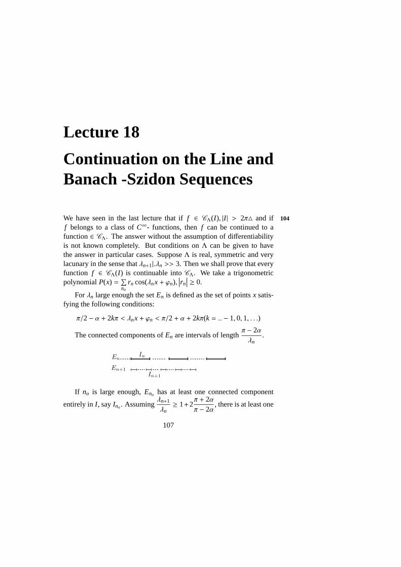
Lecture 18
Continuation on the Line andBanach -Szidon Sequences
We have seen in the last lecture that iff ∈ CΛ(I ), |I | > 2π and if 104
f belongs to a class ofC∞- functions, thenf can be continued to afunction∈ CΛ. The answer without the assumption of differentiabilityis not known completely. But conditions onΛ can be given to havethe answer in particular cases. SupposeΛ is real, symmetric and verylacunary in the sense thatλn+1|.λn >> 3. Then we shall prove that everyfunction f ∈ CΛ(I ) is continuable intoCΛ. We take a trigonometricpolynomialP(x) =
∑
no
rn cos(λnx+ ϕn),∣
∣
∣rn
∣
∣
∣ ≥ 0.
Forλn large enough the setEn is defined as the set of pointsx satis-fying the following conditions:
π/2− α + 2kπ < λnx+ ϕn < π/2+ α + 2kπ(k = .. − 1,0,1, . . .)
The connected components ofEn are intervals of lengthπ − 2αλn
.
If no is large enough,Eno has at least one connected component
entirely inI , sayIno. Assumingλn+1
λn≥ 1+2
π + 2απ − 2α
, there is at least one
107

108 18. Continuation on the Line and Banach -Szidon Sequences
connected component ofEn+1, sayIn+1, inside a connected componentIn of En (see fig.) ; we define, in that way,Ino+1. Ino+2, . . . , TakeX ∈ ∩In;thus
P(X) > sinαN
∑
no
rn, (1)
Let Λ′ = Λ − ± λ1,±λ2, . . . ,±λno−1
,∣
∣
∣ f∣
∣
∣
I= max
x∈I
∣
∣
∣ f (x)∣
∣
∣ and || f || =∑
rn, if f =∞∑
no
rn cos(λnx+ϕn),∑
rn =∑
∣
∣
∣rn
∣
∣
∣ < ∞; they are respectively105
norms in two Banach spaces, sayC (I ) andAΛ′ . (1) proves the equiva-lence of these norms for the polynomials inCΛ′(I ): sinα||P|| < |P|I ≤||P||. As the polynomialsP form a dense subset inCΛ′(I ) and inAΛ′ ,we can identifyC ′
Λ(I ) andA′
Λ: every f ∈ CΛ′(I ) can be expressed as
an element ofAΛ′ . The same result holds by adding a finite number ofterms toΛ′ (because
f ∈ CΛ(I )⇔ f = f1 + f2, f1 =n0−1∑
1
rn cos(λnx+ ϕn), f ∈ CΛ′(I )).
Thus we have prove the following proposition:
Proposition. SupposeΛ =±λn
is a real symmetric sequence which islacunary in the sense thatλn+1/λn >> 3. Then every function f∈ C (I )is the sum of an absolutely convergent Fourier-series and f is continu-able toCΛ.
A result of this type was considered by Szidon (Zygmund 1, chap.VI §6.4) who has proved that a bounded periodic function whose spec-trumΛ is lacunary in the sense of Hadamard, viz.λn+1/λn >> 1, has anabsolutely convergent Fourier series.
Definition. A sequenceΛ is said to be a Szidon sequence if for everyinterval I , f ∈ C (I )⇒ f =
∑
a(λ)eiλx and∑
∣
∣
∣a(λ)∣
∣
∣ < ∞.
We shall make a brief study of Szidon sequences and give alternatedefinitions of them by a simple lemma on Banach spaces.
Let E1 andE2 be two Banach spaces with norms|| ||1 and || ||2 and106

109
let E1 be an algebraic subspace ofE2. Moreover, for everyx ∈ E1, let||x||1 ≥ ||x||2. ThenE ′2 is imbedded inE ′1 by 〈x, x′〉1 = 〈x, x′〉2E ′2 ⊂ E ′.
By a theorem of Banach, ifE1 = E2 then the norms are equivalentandE ′1 = E ′2. Conversely, ifE ′1 = E ′2, then is it true thatE1 = E2 ? But||x||1 = sup
||x′ ||≤1
∣
∣
∣〈x, x′〉|, ||x||2 = sup||x′ ||≤1
∣
∣
∣〈x, x′〉∣
∣
∣. SinceE ′1 = E ′2 and since
||x′||2 ≥ K−1||x′||1,K > 0, we have||x||1 < K sup||x′ ||≤
∣
∣
∣〈x, x′〉∣
∣
∣ = K||x||2.
This means thatE1 is closed inE2. In order thatE1 = E2 it is necessaryand sufficient thatE1 is dense inE2. That proves
Lemma. LetE1 andE2 be two Banach spaces with norms|| ||1 and || ||2;supposeE1 is an algebraic subspace ofE2,E1 is dense inE2 and ||x||1 ≤||x||2 for every x∈ E ′1. If E ′1 = E ′2, thenE1 = E2.
Definition. We define a sequenceΛ to be aBanach sequenceif forevery intervalI and every sequenceb(λ) → 0 asλ(∈ Λ) → ∞ thereexists a functionf ∈ L1(I ) such thatb(λ) =
∫
If e−iλxdx( λ ∈ Λ).
We prove a theorem relating Banach sequences and Szidon sequen-ces, by applying the lemma.
Let E2 be the space of sequences
a(λ)
converging to zero endowedwith the norm,||a(λ)||2 = sup
λ
∣
∣
∣a(λ)∣
∣
∣.
Let E1 be the space of sequencesb(λ) with b(λ) =∫
If e−iλxdx,
where∫
I
∣
∣
∣ f (x)∣
∣
∣dx < ∞. The norm inE1 is taken as||b(λ)||1 = inf∫
I| f |
where the infimum is taken over allf for which b(λ) =∫
Ie−iλx f (x)dx.
E1 is isomorphic toL1(I )/H, whereH is the subspace ofL1(I ) orthogo-nal toeiλx.
E ′2 is the space of absolutely convergent sequencesC(λ), with thebilinear form onE2xE ′2 as〈a(λ),C(λ)〉 = ∑
a(λ)C(λ). The norm inE ′2is given by||C(λ)||2 =
∑
C(λ).E ′2 is isomorphic toAΛ.E ′1 is isomorphic to the subspaceCΛ(I ) of L∞(I ) spanned by
eiλx,with the norm ofd(λ) = ||ϕ||L∞(I ) whereϕ ∼ ∑
d(λ)eiλx. The bi-linear form giving the duality is :〈b(λ),d(λ)〉 =
∫
Ifϕ, whereb(λ) =
∫
If (x)e−iλxdx.Now the sequenceΛ is a Banach sequence if and only ifE1 = E2, 107
and a Szidon sequence if and only ifE ′1 = E ′2. A Banach sequenceΛ is

110 18. Continuation on the Line and Banach -Szidon Sequences
a Szidon sequence. In order to see that a Szidon s equence be a Banachsequence, it is sufficient to prove thatE1 is dense inE2. This is so sinceevery linear functional onE2 which is zero onE1 is zero. We can applyagain our lemma, taking (E ′1 ,E
′2) instead of (E ′2 ,E
′1).
E ′′2 is the space of bounded sequences
e(λ)
with 〈C(λ),e(λ)〉 =∑
c(λ)e(λ) and the norm||e(λ)|| = sup∣
∣
∣e(λ)∣
∣
∣.E ′′1 is isomorphic to thequotient spaceM(I )/K whereM(I ) is the space of measures with sup-port in I andK is the subspace of it orthogonal to
eiλx.
f (λ) ∈ E ′′1
when f (λ) =∫
Ieiλxdµ,dµ ∈ M(I )/K and ||b(λ)|| = inf
µ
∫
|dµ|. When
E1 = E2,E′′1 = E ′′2 . MoreoverE ′2 is dense inE ′1 (because obviouslyAΛ
is dense inCΛ(I )); thenE ′1 = E ′2 ⇒ E ′′1 = E ′′2 . We get the followingtheorem:
Theorem.The definitions of Szidon sequences and Banach sequencesare equivalent, and equivalent to the following: for every integral I andfor every bounded sequence
e(λ)
(λ ∈ Λ), there exists a measure dµwith support in I, such that e(λ) =
∫
Ie−iλxdµ(x)(λ ∈ Λ).
We have given sufficient conditions for a sequence±λn to be aBanach-Szidon sequence. Actually, Zygmund has shown (Zygmund 2)
that the conditionλn+1
λn>> 1 is sufficient. Necessary conditions involve
arithmetical properties ofλn, as it appears from the following proposi-tion (proved in (Kahane 2) ).
Let ξ1, . . . , ξp be a real numbers. Considern1ξ1+ · · ·+npξp,n j being108
integers satisfying the inequality|n1| + · · · + |np| ≤ s. If Λ is a Banach-Szidon sequence, there exists a constantA = A(λ) such that among theset ofn1ξ1 + · · · + npξp there are only [Ap log(1+ s)] of them inΛ.
Examples.Takep = 1. We cannot have more than 0(logs) points ofΛin an arithmetical progression containings terms.
Let s = 2, and p = 1,2, . . . Whatever be the sequenceξ j, wecannot have inΛ more than 0(p) points among thep2 pointsξ j + ξk,| j| ≤ p, |k| ≤ p.
The study of Banach-Szidon sequences is interesting in itself, butcan give only a partial answer to the following problem:
111
Problem. Give a relation, betweenΛ andI , such that everyf ∈ CΛ(I )is the restriction onI of a function∈ CΛ.
This problem becomes easier and has pretty good solutions if we re-placeC by the space of functions which belong toL2 on every interval,with the topology of the convergence inL2 on every interval ( (Paley -Wiener), (Kahane 2) ).


Lecture 19
Quasi-analytic classes offunctions (Quasi-analyticityD and I )
1 Quasi-analyticity and mean periodicity
We shall see presently that problems of quasi-analyticity appear in a109
natural way as problems on mean periodic functions.
1. Consider the following problem. Given a setE consider the closedspanτE( f ) of translatesfy, y ∈ E, of f . Find the conditions onf inorder thatτE( f ) = τ( f ). In other words, the problem, in a restrictedsense, is to find a relation betweenE and the spectrumS( f ) in orderthatτE( f ) = τ( f ).
2. On the other hand, the above problem suggests the following one.Let f be aC∞- function and letδ( f ) be the closed span of the deriva-tives of f . (WhenE is not a discrete set,δ( f ) is a subset ofτE( f )).Find conditions aboutf so thatδ( f ) = τ( f ). Here we require acondition involving a class ofC∞- functions, i.e. a condition onthe class and the spectrumS( f ), for example conditions of the typeKMn,S( f ), f ∈ K
Mn
.
Definition. The classK
Mn
is defined to be the class ofC∞- functionsfsuch that on every intervalI ,
∣
∣
∣ f (n)∣
∣
∣
I< KI Mn, (n = 0,1, . . .), where
Mn
113

114 19. Quasi-analytic classes of functions...
is a given sequence andKI a constant depending onI and f . C
Mn
isdefined as a class ofC∞- functions which satisfy the relation
∣
∣
∣ f (n)∣
∣
∣ <
KMn on the real line,K depending only onf .
The above two problems are closely related to quasi-analyticity.
1. In order thatτE( f ) = τ( f ) it is necessary and sufficient (condition110
of Riesz) that every measuredµ orthogonal toτE( f ) be orthogonalto τ( f ). Or again,g(y) =
∫
f (x+ y)dµ(−x) = 0 for everyy ∈ E⇒g ≡ 0. As f ∈ CΛ implies g ∈ CΛ, we have an answer to thisproblem if we have a relationRE,Λ betweenE andΛ such thatg ∈ CΛ,g(y) = 0, y ∈ E ⇒ g ≡ 0. This is nothing but a problemof uniqueness. We will be mainly interested in the case whenE isan interval.
Definition. A class of functions is called an I-quasi-analytic classif each function of the class is defined by its values onI , I beingan interval.
2. By the condition of Riesz, denoting by
g(y) = inf f (x+ y)dµ(−x),
we have δ( f ) = τ( f )⇔ [
g(n)(0) = 0 ∀n⇒ g ≡ 0]
.
When f has spectrumΛ,g ∈ CΛ. Moreover if f ∈ KMn theng ∈KMn so thatg ∈ KMn ∩ CΛ. Thus we have an answer to thisproblem if we have a relationMn,Λ such thatg ∈ KMn ∩CΛ,g(n)(0) = 0∀n ⇒ g ≡ 0. The same is true in replacingKMnby CNn.
Definition. A class ofC∞ - functions is defined as a D-quasi-analytic class if the only functiong of the class all of whosederivatives vanish at the origin is the zero function.
In Lecture 5 §2, we proved a result equivalent to the following:CΛ
is an I-quasi-analytic class if|I | > mean-period related toΛ. We givehere a far stronger result.

2. Theorem of Denjoy-Carleman 115
Theorem.LetΛ be a sequence of complex numbers such thatCΛ , C ,111
andΛ∗ andΛ− the parts ofΛ respectively to the right and to the left ofthe imaginary axis.CΛ is a quasi - analytic class whenever
|I | > 2πDmin(Λ+) or |I | > 2πDmin(Λ−).
Proof. We use the notations of Lecture 4.f ∈ CΛ, f ∗dµ = 0, f −1∗dµ =g, F(w) =
G(w)M(w)
,S( f ) = spectrum off . Denoting by∑
(dµ) and∑
(g)
the null-sets ofM(w) andG(w), we haveS( f ) =∑
(dµ)−∑
(g)∩∑
(dµ).Let Lµ and Lg be the lengths of the segments of supports ofdµ andg. According to Levinson’s theorem,L = 2π density
∑±(dµ) (∑±
is the part of∑
to the right (respectively to the left) of the imaginaryaxis). Now we use the result that ifS1 andS2 are disjoint sequences,andS = S1 ∪ S2 has a density, densityS = DmaxS1 + DminS2. ThusL = 2πDminS±( f ) + 2πDmax(S±(g) ∩ S±(dµ)); Lµ ≤ 2πDminS±( f ) + Lg.If f = 0 on (−1,0), thenLg ≤ L − 1. Hence
DminS+( f ) ≥ (Lµ − Lg)/2π ≥ 1/2π.
So if 1> 2πDminS+( f ) or 1> 2πDminS−( f ), f ≡ 0. As a translationof f does not changeS( f ), the theorem is proved.
The above theorem is stated in Levinson (Levinson, chap.II ), whenΛ is a sequence of integers, i.e.f is a periodic function; then the proofdoes not require the Carleman transform off .
2 Theorem of Denjoy-Carleman
We first study D-quasi-analytic classes in which no condition onΛ isinvolved. We shall prove a classical theorem of Denjoy-Carleman aboutD-quasi-analytic classes. It is a local property and so can be stated foran interval.
Definition. Let CI Mn be∈ class ofC∞- functions satisfying the condi-112
tions∣
∣
∣ f (n)(x)∣
∣
∣ < KMn on an intervalI ,0 ∈ I ,K depending only onf . Wesay that it is a quasi-analytic class iff (n)(0) = 0 for everyn⇒ f ≡ 0.

116 19. Quasi-analytic classes of functions...
Given a sequenceMn let MCn be the largest sequence which sat-
isfiesMcn ≤ Mn andMc
n+1/Mcnր.
Theorem of Denjoy-Carleman. CI Mn is a quasi- analytic class⇔∞∑
1
Mcn
Mcn+1
= ∞.
A variant of this theorem (stated by Denjoy without proof) is that
CI Mn is a quasi-analytic class⇔∞∑
1
1(Mc
n)1/n= ∞. The equivalence
of these two follows from the inequality:∑
∈n<∑
(∈1 · · · ∈n)1/n < e∑
∈n for ∈nց 0.
(Cf. Hary-Littlewood-Polya: Inequalities, orS. Mandelbrojt 2).
Interpretation of Mn. Consider in the plane the points (n, log Mn) andconstruct the polygon of Newton on these points. It is a convex curvem(u). The ordinate atn intersecting this curve gives logMc
n. The se-quencelog Mc
n is called the convex regularized sequence correspond-ing to log Mn. (Mandelbrojt 2).
Proof of Theorem.We can supposeI ⊃ [
0,1]
,K = Mo = 1 andMn =
Mcn. Considerϕ(x) = f (x) f (1− x) in 0 ≤ x ≤ 1 andϕ(x) = 0 elsewhere.
Since logMn is convex,Mn is the maxi≤n
(Mi Mn−i). Thus we have the
following majorization forϕ(n)(x):∣
∣
∣ϕ(n)(x)∣
∣
∣ ≤ MMn + (n1)M1Mn−1 + · · · + MnMo ≤ 2nMn
andϕ is null, with all its derivatives, at the origin. ConsiderΦ(w) =
τ(ϕ) =∫ 10ϕ(x)e−ixwdw. Integrating by parts, we have113
Φ(w) =∫ 1
oϕ(p)(x)
e−ixw
(iw)pdx and∣
∣
∣Φ(w)∣
∣
∣ < 2pMp/|w|P.
Now we introduce the functionT(r) = supp
rP/Mp. Then∣
∣
∣Φ(w)∣
∣
∣ <
1T(r/2)
. We apply Carleman’s formula forΦ(w) in the upper or lower
half plane and get∫ R logΦ(u)Φ(−u)
u2du cannot tend to−∞. Since

2. Theorem of Denjoy-Carleman 117
∣
∣
∣Φ(w)∣
∣
∣ <1
T(r/2)′, we have
∫ ∞ logT(r)r2
dr < ∞. Therefore∫ ∞ logT(r)
r2
dr = ∞ implies quasi-analyticity (Ostrowski’s form).We have logT(eσ) = t(σ) = max
n(nσ − log Mn) = max
u(σu−m(u)).
Moreover the relation betweent(σ) and m(u) is reciprocal. Indeedm(u) = max(uσ − t(σ)). Also the derivativest′(σ) andm′(u) are in-verse functions in a sense made precise by the graph. First we supposem(u)→ ∞ whenu→ ∞. Now
∫ X
e−σt(σ)dσ = −eXt(X) +∫ X
e−σt′(σ)dσ
Thus we have∫ ∞
e−σt(σ)dσ = ∞ ⇔∫ ∞
e−σt′(σ)dσ = ∞. 114
Sinceσ = m′(u) andu = t′(σ), we have the following relations:
∫ T
e−m′(u)udm′(u) = −e−m′(T)T +∫ T
∞e−m′(u)du
∫ ∞e−σt′(σ)dσ = ∞ ⇔
∫ ∞e−m′(u)du= ∞.
Betweenn ≤ u ≤ n + 1,m′(u) = log Mn+1 − log Mn and−m′(u) =
logMn
Mn+1.
∫ ∞e−m′(u)du= ∞ ⇔
∑ Mn
Mn+1= ∞

118 19. Quasi-analytic classes of functions...
∫ ∞ logT(r)r2
dr = ∞ ⇔∫ ∞
e−σt(σ)dσ = ∞.
Thus, finally we have the relation
∫ ∞ logT(r)r2
dr = ∞ ⇔∫ ∞ MC
n
MC+1n+1
= ∞.
This relation still holds whenm′(u) is bounded.We have proved that if
∑
MCn /M
Cn+1 = ∞,CI Mn is a quasi-analytic
class. Suppose∑
MCn /M
Cn+1 < ∞. Then we construct aC∞- function
with compact support which is. 0 and which satisfies the conditions∣
∣
∣ f (n)∣
∣
∣ < Mcn and f (n)(0) = 0 for everyn. To constructf it is convenient
to construct its transform.
TakeF(w) =
(
sin ∈ w∈ w
)2 ∞∏
1
sinα jw
α jw. It is an entire function of ex-
ponential type if∑
α j < ∞, α j > 0. We can majorise∣
∣
∣
sinα ju
α ju
∣
∣
∣ by 1 for
j ≥ N and we have∣
∣
∣F(u)∣
∣
∣ <
(
sin ∈ u∈ u
)2 N∏
1
1|α ju|
.
We write F(w) = C ( f ), f (x) =12π
∫ ∞−∞ F(u)eiuxdu, sinceF(u) is
rapidly decreasing. Also we have the following relations:
f (n)(x) =12π
∫ ∞
−∞F(u)(iu)neixudu
∣
∣
∣ f (n)(x)∣
∣
∣ < (α1 · · ·αn)−1∫ ∞
−∞
(
sin ∈ u∈ u
)2
du.
We takeMcn = (α1 · · ·αn)−1, i.e.αn = MC
n /MC−∞n+1 .
Thus our construction is complete.
Lecture 20
New Quasi-analytic classes offunctions
We study quasi-analyticity ofCΛ with conditions involvingΛ. First we 115
recall a result ofS. Mandelbrojt about periodic functions (Mandelbrojt1).
f ∼∑
(an cosλnx+ bn sinλnx)∑
1/λσn < ∞,0 < σ < 1∫ α
o| f | < Ke−(α−ρ), α < αo, ρ >
σ
1− σ
⇒ f ≡ 0
This signifies that if the spectrum is very lacunary, then it is notpossible to have
∫ α
o· · · very small. This leads us to find conditions
involving λn andI (α) such that∫ α
o| f | < I (α)⇒ f ≡ 0. Such functions
form a classI (α).
Definition. Given a positive functionI (α) (α > 0, I (α) ր), a class ofC∞ - functions is defined to be aI (α) quasi-analytic class when the onlyfunction of the class which satisfies the conditions
∫ α
o| f | < I (α)(α→ 0)
is the zero function.There is a connection betweenI (α) quasi-analyticity andD quasi-
analyticity. Indeed iff ∈ CI Mn,0 ∈ I and f (n)(0) = 0, forn = 0,1, . . . ,
119
120 20. New Quasi-analytic classes of functions
then by Taylor’s formula
f (x) =xn
n!f (n)(θx),
0 ≤ θ ≤ 1 and so∣
∣
∣ f (x)∣
∣
∣ ≤ xn
n!Mn which gives that
∫ α
o
∣
∣
∣ f (x)∣
∣
∣dx <
minn
αn+1
(n+ 1)!!Mn. So quasi-analyticityI (α) implies quasi-analyticityD,
when I (α) = minn
αn+1Mn
(n+ 1)!
. This function is similar to the function
T(r) introduced in the last lecture, but it seems not possible to obtain the116
Denjoy-Carleman theorem by consideringI (α).
Our problem will be to define a relation betweenΛ and I (α) suchthat EΛ is an I (α) quasi-analytic class. First we formulate the methodwe shall use in this lecture (other methods will be explained in the nextone). Supposef ∈ EΛ , E and the mean period corresponding toΛis zero; for convenience, suppose 0< Λ. Then for everyα > 0 it ispossible to find a measuredµα with support in
[ − α/2, α/2] such thatf ∗ dµα = 0, and we can assume the conditions:dµα = µ′αdx, µ′α ∈L∞, and
∫
dµα = Mα(0) = 1. Let g = − f ∗ dµα. Then (notations ofLecture 4)Gα(w) = F(w)Mα(w) andGα(0) = F(0). Suppose we have∫ α
o| f (x)| < I (α). Then ||gx||∞ < I (α)||µ′α||∞. As
∣
∣
∣Gα(0)∣
∣
∣ ≤ α||gα||, wehave
∣
∣
∣F(0)∣
∣
∣ < αI (α)||µ′α||∞. Suppose that, for an infinity ofα → 0, wecan choosedµα in such a manner thatαI (α)||µ′α||∞ → 0. ThenF(0) ≡ 0.This being true for anyf ∈ CΛ, we take primitives off instead off (x)andF′(0) = 0 etc. ThusF ≡ 0 and f ≡ 0. Thus we are able to formulateour condition as follows:
Suppose that to eachα > 0 we associateµ′α ∈ L∞ with support in[ − α
2,α
2]
such that∫
µ′α = 1 and∫
eiλxµ′αdx = 0 for everyλ ∈ Λ. If
lim inf α→0αI (α)||µ′α||∞ = 0, thenCΛ is anI (α) quasi-analytic class.We shall use this condition in the following form.
Lemma. Suppose that to eachα > 0 we associate an entire function117
Mα(w) of exponential type≤ α
2, such that Mα(u) ∈ L1,Mα(0) = 1,
121
Mα(Λ) = 0. If lim infα→o
αI (α)∫
|Mα(u)| = 0, thenCΛ is an I(α)- quasi-
analytic class.
We apply the above condition in the case whenΛ is a real symmet-
ric sequence,Λ = ±λn such that∑ 1λn
< ∞. To construct the func-
tion Mα(w) we take the canonical productC(w) =∞∏
1
(
1− w2
λ2n
)
and take
Mα(w) = C(w)∞∏
o
sinα jw
αwj
with 4∑
α j = α. we take this additional
factor sinceC(w) does not behave well real axis.Mα(w) is a function ofexponential type
α
2, sinceC(w) is of type 0. Now we have to construct
αn in such a manner thatMα(u) ∈ L1. To do this we first try to majoriseMα(w). Supposeλn ≤ u ≤ λn+1. We have the following calculations:
∣
∣
∣Mα(u)∣
∣
∣ =
n∏
1
(
u2
λ2m− 1
) ∞∏
n+1
(
1− u2
λ2m
) ∞∏
o
(
sinα ju
α ju
)2
<u2n
λ21 · · · λ
2n
1
α21 · · ·α
2nu2n
min
(
1,1
α2ou2
)
(we already used such a majorization, for∞∏
o
sinα ju
α ju, in Lect. 19, §2).
∫ ∞
o
∣
∣
∣Mα(u)∣
∣
∣du=∫ 1
o+
∫ ∞
1<
(
1+1
α2o
)
(maxn
(λ1α1, . . . , λnαn))−2.
This majorization is not useful if∑ 1λn= ∞, because the second
member is∞ (if not, we would have (α1 · · ·αn)1/n >K
(λ1 · · · λn)
1/n
>Kλn
,
and the equiconvergence of∑
αn and∑
(α1 · · ·αn)1/n, which we stated inLect. 19 §2, leads to a contradiction). To get a result, we must suppose∑ 1λn
< ∞. Choose a sequenceln, ln → ∞, such that∑∞
1lnλn
< l8
and takeαo = α/8, α j = l jα/λ j . Then 4∑∞
o α j < ∞ and maxn
(λ1α1 · · · 118
λnαn) = maxn
(l1 · · · lnαn). This is finite sinceln → ∞. (The expression

122 20. New Quasi-analytic classes of functions
(maxn
(l1 · · · lnαn))−2 is of the same form as maxrn/Mn which we have
seen already). Thus we have∫ ∞
−∞|Mα| < Const.(max
n(l1 · · · lnαn))−2α−2;
Mα(w) = 0 onΛ andMα(w) is of type≤ α. Now the condition lim infα→0
αI (α)∫
Mα(u) = 0 follows from lim infα→0
I (α)/αminn
(l1 · · · lnαn)2= 0. By
changing the firstl j if necessary and by replacingl j by kl j(k > 1) forsufficiently large j we have the following condition forCΛ to be I (α)quasi-analytic.
Theorem.SupposeΛ = ±λn,0 < λ1 < λ2 · · ·∞∑
1
1n
λnwith 1n ր ∞ and
lim infα→0
I (α)αmin
n((l1 · · · lnαn)−2
< ∞. ThenCΛ is an I(α) quasi-analytic
class.
When λn is not a sequence of real numbers, but symmetric and∑ 1|λn|
< ∞, the same method can be used with the additional hypothesis
that∣
∣
∣λ j
∣
∣
∣/ j1+∈ր so as to have a good majorization of∏
∣
∣
∣1 − u2/λ2j
∣
∣
∣ and
in this case∣
∣
∣
∏
(1+u2
|λ j |2)∣
∣
∣ < kmax(k2u)2n/|λ1 · · · λn|2 (see (Kahane 1)).
The condition|λ j |/ j1+∈ ր is a condition of regularity.Our condition ofI (α)-quasi-analyticity givesS. Mandelbrojt’s the-
orem. Suppose∑ 1λτn
< ∞,0 < σ < 1. Take 1n = λ1−σn . Thus
∑
1n>n
1− σσ
1/1σ(1−σ) < ∞. Takeλn ր and so 1n ր,1σ
1− σn /n → ∞
and
maxn
rn
l1 · · · ln< max
n
(( σr1−σ )n)1−σ)/σ
(n!)(1−σ)/σ< e
(1− σ)ro rσ/1−σ
Takingα = 1/r we have quasi-analyticity wheneverI (α) < α2e
1− σσ119

123
ασ/1−δ.Again, we can derive a condition ofD-quasi-analyticity forCMn∩
CΛ. We have seen thatCI Mn ∩ CΛ is D-quasi-analytic withI (α) =
minn
αn+1
(n+ 1)!Mn. Thus it is sufficient that min
n(α2nM2n/(2n + 1)!) <
minn
(l1 · · · lnαn)2 for an infinity of α, α → 0. This means that the re-
verse inequality does not hold forα > αo. In other words, takingα = 1/r,max
n(r2n(M2n/(2n+ 1)!)−1) ≤ max
nr2n(l1 · · · ln)−2 does not hold
for r > ro. Now we use the following lemma.
Lemma. Let An and Bn be two positive sequences with Bn+1/Bn ր.Then
Bn ≤ An, (n > no) ⇐⇒ maxn
rn/Bn ≥ maxn
rn/An(r > ro).
For the proofC f . (Mandelbrojt 3, p.7 and p. 18).
Taking An =M2n
(2n+ 1)!, Bn = (l1 · · · ln)2 our condition becomes:
M2n
(2n+ 1)!≥ (l1 · · · ln)2 does not hold forn > no (whatever we choose
no). ReplacingMn by kMn, we get:
Theorem.We make the same assumptions aboutΛ, λn,1n as in theabove theorem; I is an arbitrary interval.
If limn→∞
infM2n
(2n+ 1)!(11 · · ·1n)2> 0 CΛ ∩CI Mn
is a D-quasi-analytic class.


Lecture 21
Applications of the Formulaof Jensen and Carlemanto quasi-analytic ClassesDand I (α)
1 Principle of the method
We give here an alternative method for obtaining conditions of quasi-120
analyticity. This method is applicable to bounded mean-periodic func-tions (for quasi-analyticityI (α) and for mean periodic functions belong-ing to a classCMn (for quasi-analyticityD). Moreover, it is easilyseen that the method can be applied to those classes of bounded func-tions on the real line whose Carleman transforms (in the classical sense)are meromorphic, either on the whole plane or at the right (left) of theimaginary axis (for example, almost periodic functions whose spectrumhave no finite point of accumulation on the line (resp. on a half line ) ).
Following a method ofB. Levin, we takeI (α) = e−αr(α) wherer(α)is a decreasing function ofα which is∞ on [0, α∞] and continuous withvalues from∞ to ro on (α∞, αo],0 ≤ α∞ < αo. We denotelg/α(r) theinverse function, defined on [ro,∞), such thatα(∞) = α∞.
Let now∫ α
o| f | ≤ I (α) (0 < α < αo); if α∞ , 0, this meansf = 0 on
125

126 21. Applications of the Formula of Jensen and...
[0, α∞]. Let F(w) be the Carleman transform off (Lect. 6, §3).
F(w) =
o∫
−∞
f (x)eixwdx for v > 0
F(w) = −∞
∫
o
f (x)e−xwdx for v < 0.
We have the following majorizations:121
|F(w)| = |∞
∫
o
f (x) e−ixw dx| ≤ |α
∫
o
| + |∞
∫
α
|
≤ I (α) + Ke−α|v|
|v| v < 0
| F(w) | ≤o
∫
−∞
| f (x) | exv| dx <K|V| , v > 0.
For a givenw we can chooseα as we want and we takeα = α(|v|),|v| = r(α). Thus the above majorization forv < 0 reduces to the follow-ing one:
|F(w)| <(
1+K|v|
)
e−αr(α) ≤(
1+K|v|
)
e−|v|α(|w|).

1. Principle of the method 127
This relation permits us to have the following lemma:
Lemma 1. The set of bounded functions inCΛ , C is an I(α) quasi-analytic class, with I(α) = e−αr(α)as soon as the following relation issatisfied:
log |F(w)| < − log |v|, v > 0 (w = u+ iv = reiθ)
log |F(w)| < − log|v||1+ v| − |v|α(r), v < 0
F(w) meromorphic with simple poles atΛ.
⇒ F ≡ 0
Let now f ∈ CMn ∩ CΛ,CΓ , C and f (n)(0) = 0 for everyn.ThenF(w) satisfies the following relations:
F(w) =
o∫
−∞
f (n) (x)e−ixw
(iw)n dx v> 0
|F(w)| < K Mn
|w|n
o∫
−∞
evx dx=K Mn
|v| rn v > 0
|F(w)| < K Mn
|v|rn v < 0
We have seen in Lecture 7 (sincef is bounded) thatF(w) is a mero-morphic function with real simple poles atΛ and from the above in-
equalities we have|F(w)| < infnK Mn
|v| rn .
Thus we have the following Lemma: 122
Lemma 2. The classCΛ ∩CMn,CΛ , C is a D-quasi-analytic classas soon as the following relation is satisfied:
F(w) if meromorphic with simple poles atΛ
log |F(w)| < − log |v| − S(r)
with S(r) = maxn
(n log r − log Mn)
⇒ F ≡ 0

128 21. Applications of the Formula of Jensen and...
2 Application of Jensen’s and Carleman’s formulae
Application of Jensen’s formula: Here we assumeΛ = ±λn. Defini-tions ofn(r), D(r), D. are given in Lect. 10. §1.
We suppose thatF(w) satisfies the majorizations of Lemma 1 andthatF(w) . 0. First, Jensen’s formula gives the following majorization:(Lecture 10.§2)
−2
r∫
o
n(t)t
dt ≤ 12π
2π∫
o
log |F(reiθ) | dθ − log | F(0) |
Division of F(w) by wp will not alter the conditions of Lemma 1 andso we can takeF(0) , 0. Using the majorizations of Lemma 1 in theabove inequality, we have
−2 r D (r) < −1π
rα(r) − 12
log r + 0(1)
and soα(r) < 2πD(r) for sufficiently larger.This relation gives us the following theorem:
Theorem 1. The set of bounded functions ofCΛ , C is an I(α) quasi-analytic class, with I(α) = e−αr(α) as soon asα(r) ≥ 2πD(r) for aninfinity of values of r→ ∞.
Remarks.1) If α(∞) > 2πD, the above theorem gives that the set of123
bounded functions ofCΛ , C is a quasi-analytic class I.|I | = 1,whenever 1> 2πD.. This result is contained in Levinson’s theorem(Lecture 19.§1).
2) If D(r) ≤ D. for an infinity of values ofr → ∞ it is sufficient to haveα(∞) = 2πD. to apply the above theorem and thus, in this case, weget a precision of Levinson’s theorem.
3) The above Remark (2) applies to the case of odd integers where we
have D. =12
, then also the case of even integers. But if we add
±1 to Λ the result ceases to apply. Indeed, there exists a function
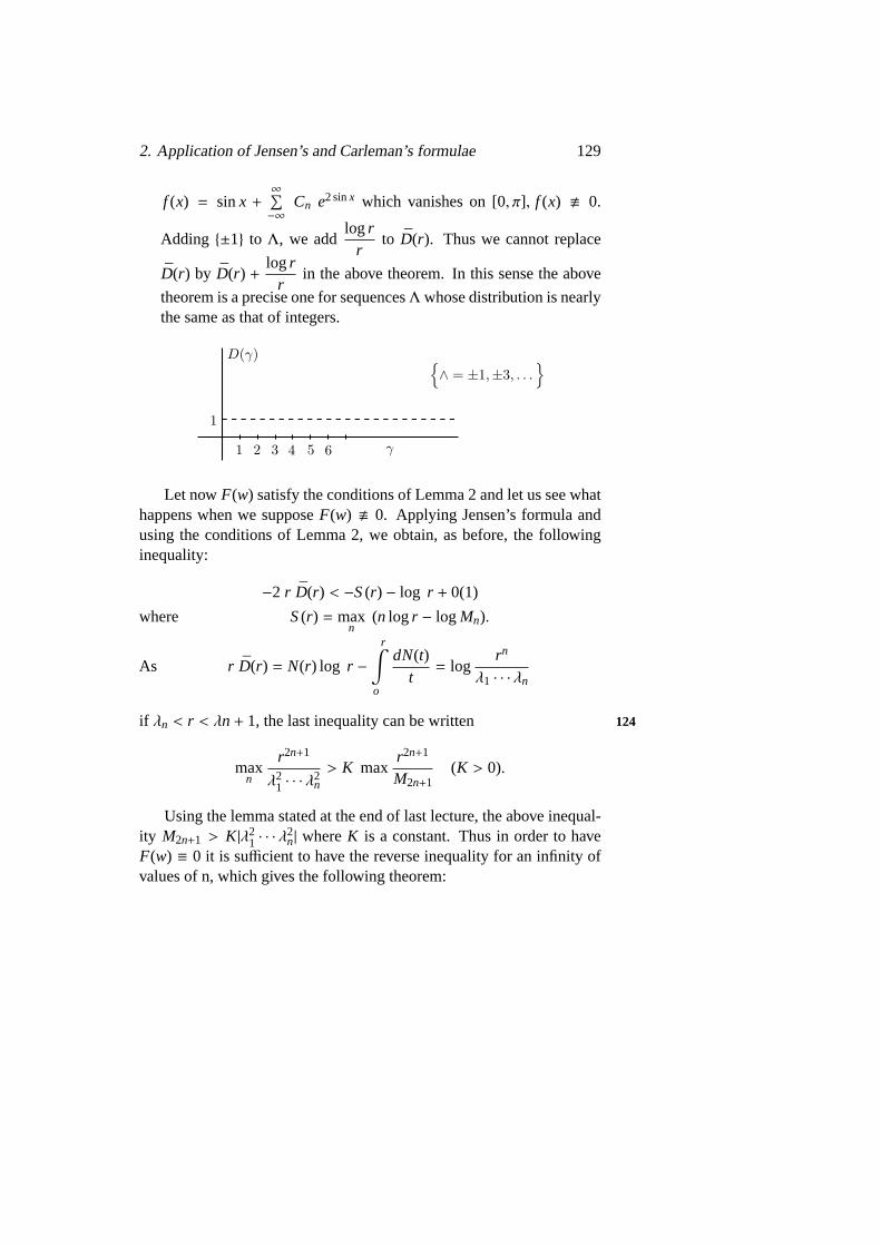
2. Application of Jensen’s and Carleman’s formulae 129
f (x) = sinx +∞∑
−∞Cn e2 sinx which vanishes on [0, π], f (x) . 0.
Adding ±1 to Λ, we addlog r
rto D(r). Thus we cannot replace
D(r) by D(r) +log r
rin the above theorem. In this sense the above
theorem is a precise one for sequencesΛwhose distribution is nearlythe same as that of integers.
1 2 3 4 5 6
1
Let nowF(w) satisfy the conditions of Lemma 2 and let us see whathappens when we supposeF(w) . 0. Applying Jensen’s formula andusing the conditions of Lemma 2, we obtain, as before, the followinginequality:
−2 r D(r) < −S(r) − log r + 0(1)
where S(r) = maxn
(n log r − log Mn).
As r D(r) = N(r) log r −r
∫
o
dN(t)t= log
rn
λ1 · · · λn
if λn < r < λn+ 1, the last inequality can be written 124
maxn
r2n+1
λ21 · · · λ
2n> K max
r2n+1
M2n+1(K > 0).
Using the lemma stated at the end of last lecture, the above inequal-ity M2n+1 > K|λ2
1 · · · λ2n| whereK is a constant. Thus in order to have
F(w) ≡ 0 it is sufficient to have the reverse inequality for an infinity ofvalues of n, which gives the following theorem:

130 21. Applications of the Formula of Jensen and...
Theorem 2. CΛ ∩ CMn is a D -quasi-analytic class as soon as thefollowing condition is satisfied:
lim infn→∞
M2n+1
λ21 · · · λ
2n= 0.
Remark. The above condition is simpler and more precise than the con-dition of D - quasi-analyticity obtained in the last lecture. However, thiscondition is applicable only whenΛ is real and it involvesCMn insteadof CI Mn. But the latter inconvenience can be suppressed whenever = 0, by the use of the theorem of continuation of Lecture 17.
Using a result proved in the next lecture, we can obtain that theabove condition is also necessary forD-quasi-analyticity, whenΛ issufficiently lacunary.Application of Carleman’s formula: We assume now nothing aboutthe negative part ofΛ; the functionsn+(r),D+(r) are related to the posi-tive part ofΛ.
SupposeF(w) satisfies the condition of Lemma 7 and letF(w) . 0.The application of Carleman’s formula in the right half-plane gives125
r∫
(1/t − t/r2) dn+(t) >12π
r∫
(1/v2 − 1/r2)vα(v) dv+ 0(1).
Now, if D+(r) is bounded, integrating by parts, this reduces∞:
r∫
2π D+(t) − α(t)t
dt > 0(1).
Thus we have the following theorem:
Theorem 3. The class of bounded functions ofCΛ , C is an I(α) quasi-analytic class, with I(α) = e−αr(α) when D+. < ∞ and
lim supr→∞
r∫
α(t) − 2πD+(t)t
dt = ∞.
2. Application of Jensen’s and Carleman’s formulae 131
Suppose now thatF(w) satisfies the conditions of Lemma 2 and
F(w) . 0. Setw′ = ie−iπawa, with12≤ a ≤ 1. We takeF1(w′) =
F(w).F1(w′) is meromorphic in the right half-plane having poles only
on the line argw′ =π
2− πa and the distribution of these poles is
N1(ρ) = N+(ρ
1a). Moreover we have
log |F1(w′)| < − log |ρ 1a sin
2θ′ − π2a
| − S(β1a ).
(w′ = ρ eiθ′). Carleman’s formula applied toF1(w′ + 1) in the righthalf-plane gives us the following inequality:
lim supρ→∞
ρ∫
(S(τ1a ) − π sinπaN+(τ
1a )
dτ
τ2< ∞
This relation gives us the following theorem:
Theorem 4. CΛ ∩CMn is a D - quasi - analytic class when
N+(r) = 0(ra) and lim supr→∞
r∫
S(t) − π sinπaN+(t)t1+a
dt = ∞
with S(r) = maxn(n log r − log Mn),12≤ a ≤ 1.
Remarks.1) Fora = 1, we get the condition of Denjoy-Carleman. 126
2) If∞∫ N+(t)
t3/2dt < ∞,CΛ ∩ CMn is D-quasi-analytic ifC
√Mn is
D-quasi - analytic.
WhenF(w) is not meromorphic in a right or left half-plane we can-not apply either Carleman’s or Jensel’s formula. Partial results in thisdirection can be got by applying a formula due to Mandelbrojt and Mac-Lane (Kahane 1).


Lecture 22
Reciprocal theorems aboutquasi-analyticity D and I (α)
In the Lectures 20 and 21, we gave sufficient conditions in order thatCΛ 127
should be anI (α) quasi-analytic class, orCΛ∩CI Mn respCΛ∩CMna D-quasi-analytic class. We stated that ifΛ is sufficiently lacunary,some of these conditions are necessary. In order to know whether oursufficiency conditions are good (i.e., whether it is not possible to relaxthem very much), and, if possible, to find necessary and sufficient con-ditions, we shall construct a functionf ∈ CΛ “as small as possible” nearthe origin. Actually, we want first to havef (n)(0) = 0(n = 0,1, . . .) andsupx| f (n)(x)| increasing as slowly as possible.
We saw in the Lecture 21 that the smallness at infinity ofF(w), theCarleman transform off , is related to the smallness off near the origin.Therefore, it is natural to takeF(w) “as small as possible” at infinity.SupposeΛ = ±λn to be symmetric and real. Then the Carleman trans-
form of every f ∈ CΛ is the product ofFo(w) =∏
(1 − w2
λ2n
)−1 by an
entire function. With convenient hypothesis onΛ we shall constructfo ∈ CΛ, whose Carleman transform isFo(w). It is natural to expect thatf0 is the function we want.
We supposeΛ = ±λn to be symmetric, real and lacunary in the
same thatλn+ 1λn
> K > 1. We denote by∑
(Ak
w− λk− Ak
+λk) the polar
133

134 22. Reciprocal theorems about quasi-analyticity D andI (α)
part ofR0(w) =∏
(1− w2
λ2j
)−1; thenAk = −λk2
∏
j,k(1− λk
λ2j
)−1. We define128
f0(x) = 2∑
Ak sinλk x; indeed, if∑ |Ak| < ∞ (and the following calcu-
lation proves that it is realised),Fo(w) is the Carleman transform offo.We now try to get a majorization for| f (n)
0 (x)|.
| f (n)o | < 2
∞∑
1
|Ak|λnk
|Ak| =λk
2
λ21 · · · λ
2k
λ2kk
k−1∏
j=1
|λ2
j
λ2k
− 1|−1|∞∏
j=k+1
1− |λ2
k
λ2j
−1
|Ak|λ2kk < Cλ2
1 · · · λ2k−1|λ
3k
| f (2n−1)o | < 2C
∞∑
k=1
λ21 · · · λ
2k λ
(2(n−k)k
= 2C λ21 · · · λ
2n
n−1∑
1
λ2(n−k)k
λ2k+1 · · · λ
2n
+ 1+∞∑
n+1
λ2n+1 · · · |λ
2k
λ2(k−n)k
< C1 λ21 · · · λ
2n
and| f (2n)0 | < C1 λ
2n · · · λ2
1 λn+1 by a similar calculation. We takeM2n−1 =
λ21 · · · λ
2n andM2n = λ
21 · · · λ
2n λn+1. Then we havefo ∈ CMn.
Moreover f (n)0 (0)(n = 0,1, . . .). For, if N were the first integer such
that f (N)0 (0) , 0, we would have, forv > 0.
F0(w) =f (N)o (0)(iw)N
=f (N+1)0 (0)
(iw)N+1+
0∫
−∞
f (N+2)0 (x) (ix)−N−1e−ixwdx
and limv→∞
(−v)NF(−iv) = f (N)(0) , 0; since∏
(1 +v2
λ2k
) increases more
rapidly than any polynomial, this is impossible.
In Lecture 21, we found that lim infn→∞
M2n
λ21 · · · λ
2nλn+1
= 0 is a sufficient
condition for theD-quasi-analyticity ofCΛ ∩CMn. The properties off gives us the following result:
22. Reciprocal theorems about quasi-analyticity D andI (α) 135
Theorem 1. If Λ = ±λn is real, symmetric and lacunary in the sense129
thatλn+1
λn> K > 1, necessary and sufficient condition in order that
CΛ ∩CMn should be D-quasi-analytic is that either
1) lim infn→∞
M2n
λ21 · · · λ
2nλn+1
= 0, or
2) CΛ∩CMn does contain the function fo whose Carleman transform
is Fo(w) =∏
(1− w2
λ2n
)−1.
Using Taylor’s formula as in Lecture 20, § 1, we have
α∫
o
| fo | < C1
α∫
o
x2n−1
(2n− 1)!λ2
1 · · · λ2n dx= C1
α2n
(2n)!λ2
1 · · · λ2n
Henceα
∫
o
| fo| < C1 minn
(α
(2n)!λ2
1 · · · λ2n) (1)
We saw (Lect. 20) thatCΛ is anI (α) quasi-analytic class if∑ lnλ<
∞ and
lim infα→∞
I (α)αmin(l1 · · · lnαn)2
< ∞ (2)
(1) shows that this condition cannot be very much relaxed; for ex-
ample, we cannot replace∑ lnλ< ∞ by ln =
λn+1
2n.
If λn+1/λn is bounded, the condition is invariant by a change oflninto ln+p, and also intoln+p; then, if it holds withI (α) it still holdswith α−2p I (α). That is no longer true if we assume
∑ λn
λn+1< ∞ (3)
For, we can take in (2)ln = ln−1; but, according to (1), we cannotln = λn+1. This remark will lead us tu show thatf0 is “the smallest”

136 22. Reciprocal theorems about quasi-analyticity D andI (α)
function∈ CΛ near the origin, in the sense that
f ∈ CΛ, lim infα→0
α∫
o
| f | /α
∫
o
| fo| < ∞ (4)
implies f = K fo,K constant.130
We suppose (3) and (4). SinceΛ is a sequence of Banach - Szidon,f is bounded. LetF(w) be the Carleman transform off ; we have|F((u+
iv)| < K|v| (Lect. 7); hence
|F(w) (w− λn) (w− λn+1)| < K(λn+1 − λn)
on the circle of diameter (λn, λn+1), andF(w) is uniformly bounded out-side the discs of radius 1 around the±λn. Suppose,f / fo is not a con-stant. ThenA(w) = F(w)/Fo(w) is an entire function which is not aconstant. SinceF−1
o is of exponential type zero, andF is bounded out-side our discs,A(w) is also of exponential type zero; therefore, it hasat least one zerow1. Let F(w) = (w − w1) F1(w). Without restriction,we can supposef (0) = 0; then the differential equationf = i f ′1 + w1 f1has one solution such thatf ′1(0) = f1(0) = 0 and, using the formulae ofLecture 6, § 2, we see thatF1(w) is the Carleman transform off1. Now,
using the trivial inequalityα∫
o| f1| < α
α∫
o| f ′1|, we get, forα small enough,
α∫
o
| f | >α
∫
o
| f ′1| − |w1|α
∫
o
| f1| >12
α∫
o
| f ′1| >1
2α
α∫
o
| f1|
This inequality, together with (4), shows thatf1/ fo is not a consis-tent. We can iterate our argument and getf2 ∈ CΛ, f3 ∈ CΛ, f3 . 0
α∫
o
| f | > 12α
α∫
o
| f1| >1
4α2
α∫
o
| f2| >1
8α3
α∫
o
| f3|
Taking into account (1) and (4), we get
lim infα→o
(
α∫
o
∣
∣
∣
∣
f3|/
minn
(α2n−3
(2n)!λ2
1 · · · λ2n
))
= 0,

22. Reciprocal theorems about quasi-analyticity D andI (α) 137
which is in contradiction with the fact thatCΛ is anI (α) quasi-analytic 131
class whenever lim infα→oI (α)
αmin(λ1 · · · λnαn+1)2= 0. We conclude that
f / fo must be a constant. We express the result in the following way.
Theorem 2. If Λ = ±λn is real, symmetric and very lacunary in the
sense that∑ λn
λn+1< ∞, a necessary and sufficient condition in order
thatCΛ should be an I(α) quasi-analytic class is
lim infα→∞
I (α)/
α∫
o
| fo|
= 0, fo
being defined in Theorem1. Every time f∈ CΛ and
lim infα→o
(
α∫
o
| f |/∞
∫
o
| fo|)
< ∞, f / fo
is a constant.
Remark. It is easy to extend this result. Indeed, iff ∈ CΛ and
lim inf α→o
(
αpα∫
o| f |
/
α∫
o| fo|
)
< ∞, f is a linear combination (with con-
stant coefficients) of fo, f 1o , . . . , f (p)
o . It means not only thatfo is “thesmallest” function∈ CΛ near the origin, but also the linear combina-tions of fo and its derivatives are “smaller” than any otherf ∈ CΛ.


Lecture 23
Mean Periodic Functions ofSeveral Variables
In the case of several variables instead of considering continuous func- 132
tion, we considerC∞-functions. It would also be possible to considerdistributions.
We consider the spaceE = E (Rn), f ∈ E , f (x) = f (x1, . . . , xn), x =(x1, . . . , xn) ∈ Rn. The monomial exponentials are of the formxi1
1 · · · xinn
ei(λ1x1+···+λnxn) and the polynomial exponentials are of the formP(x1, . . . ,
xn) ei(λ1x1+···+λnxn).A function f is mean periodic ifτ( f ) , E (Rn). An equivalent defi-
nition is that f is mean periodic if there exists aµ ∈ E ′, µ , 0, µ ∗ f = 0.
Problem 1. If f is mean periodic, can we assert thatf belongs to thespan of monomial exponentials belonging toτ( f )?
The answer is in the negative (Ehrenpreis 1). InR2, let f = x1 + x2.The monomial exponentials inτ( f ) are constants.
Problem 2.Let f ∈ τ ⊂ E , τ a closed subspace invariant under transla-tions. Is f ∈ span of polynomial exponentials∈ τ?
Solution is not known.
Problem 3.Supposef ∗ µ = 0, µ ∈ E ′(Rn). Is f ∈ span of polynomial
139

140 23. Mean Periodic Functions of Several Variables
exponentialsQ with Q ∗ µ = 0?
This is answered in the affirmative (Malgrange 1).Let V(µ) denote the set of linear combinations of polynomial expo-
nentials verifying the equationQ ∗ µ = 0.
Letvν be the distribution symmetric to the distributionν. If
vν ∗Q = 0133
for every polynomial exponentialQ verifying the equationQ ∗ µ = 0and f ∗ µ = 0, then is
vν ∗ f = 0? This problem is put in the following
form:(vν ∈ (V(µ)⊥), f ∗ µ = 0 ⇒ ν ∗ f = 0.
Theorem 1. f ∗ µ = 0⇒ f ∈ V(µ). This theorem follows from parts a)and e) of the following theorem (Malgrange1).
Theorem 2. The following conditions are equivalent:
a)vν ∈ [V(µ)]⊥
b) Every exponential polynomialQ satisfying the equationQ ∗ µ = 0also satisfies the equationQ ∗ ν = 0. In other words,V(µ) ⊂ V(ν).
c) C (µ)/C (ν) is an entire function.
d) C (µ)/C (ν) is an entire function of exponential type.
e) ν ∈ µ ∗ E ′ = closed ideal generated byµ.
We recall thatF(w) is of exponential type if|F(w)| < A eB|w|, |w| =|w1| + · · · + |wn|. We prove the theorem in four steps, inserting the lem-mas and propositions which we require in the four steps, inserting thelemmas and propositions which we require in the proof of each step.
1. a) ⇐⇒ b). Indeedνν ∈ [V(µ)]⊥ ⇒ v
ν.Q = 0 for every exponentialpolynomial Q satisfyingQ ∗ µ = 0, and so
νν ∈ [V(µ)]⊥ ⇐⇒
vν ∗ τaQ = 0 for every translateτaQ of Q.
In other words,vν ∈ [V(µ)]⊥ ⇐⇒ Q ∗ ν = 0 for every exponential
polynomialQ satisfyingQ ∗ µ = 0.

141
2. b ⇐⇒ c). Let C (µ) = M(w); w = (w1, . . . ,wn). According toSchwartz’s theory of the Fourier transforms of distributions,b) isequivalent to the relation:C (µ)C (Q) = 0⇒ C (ν)C (Q) = 0. Soc)→ b).
Now C (Q) is a distribution with support atλ and we denote it by 134
Dλ. b) gives us thatm.Dλ = 0⇒ N.Dλ = 0, whereM.Dλ is the productof the distributionsM andDλ and so alsoN.Dλ. To prove thatb) ⇒ c)we use the following lemma:
Lemma. Let M and N be analytic at the origin. In order that N/M beanalytic at the origin it is necessary and sufficient that for every distri-bution D with support at origin M.D = 0⇒ N.D = 0.
Necessity is obvious. To prove the sufficiency, consider the ringAof formal power-series
∑
ai1,···in xi11 · · · x
inn . It is a topological ring with
the simple convergence of the coefficients. It is locally convex and itsdual A ′
= E ′o is the space of distributions with support at the origin.The scalar product is given by
〈D,∑
· · · 〉 =∑
ai1···in〈D, xi1 · · · x
inn 〉.
We use the following result proved in (CartanX, p.7).
NM
is analytic at 0⇐⇒ NM∈ A .
Thus we have to prove thatN ∈ MA , the ideal generated byM. Weuse the fact that this ideal is closed (CartanXI, p.7). Then it is sufficientto prove thatD ∈ (MA )⊥ ⇒ 〈D,N〉 = 0. But 〈D,MK〉 = 〈M.D,K〉, sothat D ∈ (MA ) ⇐⇒ M.D = 0. As we assumeM.D = 0 ⇒ N.D = 0,and〈D,N〉 = 〈N.D,1〉, we have provedN ∈ MA , thenN/M is analyticat the origin.
Sinceb) gives thatM.Dλ = 0 ⇒ N.DΛ = 0 we have, by the abovelemma,N/M analytic at every pointλ.
3. c) ⇐⇒ d) is a consequence of the following theorem: (Mal-grange) (Ehrenpreis 1).
Theorem of Lindelof-Malgrange-Ehrenpreis: If F and G are func-135

142 23. Mean Periodic Functions of Several Variables
tions of exponential type and F/G is entire, then F/G is also a functionof exponential type.
In this proof, L. Ehrenpreis used a theorem on minimum modules.On the other hand, Malgrange’s proof is directly inspired from that ofLindelof.
We have to return to analytic functions of one variable.
SupposeF(w) = wPeaw∞∏
1(1− w/λ j)ew/λ j . This form ofF(w) need
not imply thatF(w) is of exponential type. For example, the inverseof the classicalΓ- function is not of exponential type. Lindelof gave acharacterization of entire functions of exponential type. Let the zeros ofF(w) be arranged in such a fashion that|λ j+1| ≥ |λ j |. ThenF(w) is of
exponential type if and only ifn|λn|= 0(1) and
∑
|λi |<|K1/λi = 0(1) for all
K. Using this characterization, one proves in the case of one variablethatF(w)/G(w) is of exponential type. Malgrange gave a refinement ofthis characterization.
Proposition 1. Let F(w) be an entire function with F(0) , 0 and|F(w)| < A eB|w| and letλn be the zeros of F(w). Then
a)nλn|
<C|F(0)| , b) |a+
n∑
1
1λ j| < D
|F(0)|2;
C = C(A, B),D = D(A, B).
Conversely, ifnλn
< eand|a+p∑
1
1λ j| < D for everyn andp, then
F(w) = eaw∞∏
1
(
1− wλ j
)
ew/λ j
is an entire function and
|F(w)| = |F(w)/F(0)| < A eB|w|,A = A(c,D) andB = B(C,D).
For the first part of the proposition,a) follows easily from Jensen’s136
formula: b) is more involved. The second part follows from some cal-culations (Malgrange).

143
Proposition 2. Let |F(w)| < A eB|w| with F(0) = 1 and let |G(w)| <A′ eB′ |w| with G(0) = 1. Suppose H(w) = F(w)/G(w) is an entire func-tion. Then|H(w)| < A′′eB′′ |w| with A′′ and B′′ depending only on A,A′, Band B′.
Proposition 2 is an immediate consequence of Proposition 1.Now the proof of Lindelof theorem for several variables follows eas-
ily from Proposition 2.Suppose|F(w1 · · ·wn)| < A eB(|w1|+···|wn|),
|G(w1, . . . ,wn)| < A′ eB′(|w1|+···+|wn|) andH(w) = F(w)/G(w)
is an entire function. We fixw1 · · ·wn such that|w| = |w1|+ · · ·+ |wn| = 1and takeFw(δ) = F(δw1, . . . , δwn),Gw(δ) = G(δw1, . . . , δwn). Then byProposition 2,|Hw(δ)| < A′′eB′′ |δ|.
Hence, for anyw = (w1, . . . ,wn), we have|H(w)| < A′′eB′′ |w| (be-causeH(w) = Hw/|w|(|w|)).

Lecture 24
Mean Periodic Functions ofSeveral Variables(Continuation)
We complete the proof of the main theorem of the last lecture. 4,d)⇐⇒ 137
e.d) C (ν)/C (µ) is an entire function of exponential type.e) ν ∈ µ ∗ E ′, the closed ideal generated byµ in E ′.Now e) ⇐⇒ c) is evident and sincec) ⇐⇒ d),e) ⇒ d). The proof
of d)⇒ e) is involved.Let QY ′ be the space of Fourier-transforms of distributions inE ′.
Let M,N ∈ QY ′ and supposeN/M is of exponential type. Moreover
suppose it is possible to show that∂ M∂ w1
N ∈ C (µ ∗ E ′). Then we can
prove thatd) ⇒ e), because we can iterate the same process with each
variable and get∂ M∂ w2
∂ M∂ w1
N ∈ C (µ ∗ E ′) etc., and finally (P(x)µ) ∗ ν ∈µ ∗ E ′, for every polynomialP(x). Using the result that ifµ , 0 it ispossible to find a sequenceP(x) andλ ∈ Rn such thatP(x)µ → δλ we
find thatδλ ∗ ν ∈ µ ∗ E ′, i.e. ν ∈ µ ∗ E ′. Now we can write∂ M∂ w1
N =
1M∂ M∂ w1
NM. To prove that∂ M∂ w1
N ∈ C (µ ∗ E ′) it is sufficient to prove
the following conjecture (true in the case of one variable).
145

146 24. Mean Periodic Functions of Several Variables (Contd.)
Conjecture.1M∂ M∂ w1
NM ∈ QY ′, whenM.N ∈ QY ′ andNM
is entire.
Unfortunately we are not able to prove this conjecture. But to prove thatd) ⇒ e) it is sufficient (as indicated by Malgrange) to prove only thefollowing proposition:
Proposition 1. P,R ∈ QY ′ and P/Q entire implies that1Q∂ Q∂ w1
P Q2138
(0,w2, . . . ,wn) ∈ QY ′.
The idea of the proof is to majorise1Q∂ Q∂ w1
in the same way as
M′(w)M(w)
in Lecture 5, §1, and to use Proposition 1 of the last lecture
(B.Malgrange).
Definition. H(µ) is the set of distributionτ such thatτ ∗ ν ∈ µ ∗ E ′, foreveryν with C (ν)/C (µ) entire.
Theorem.H(µ) is dense inE ′.
Suppose this theorem is proved. Allowingτ → δ we haveν =limτ∈H(µ)τ→δ
τ ∗ ν andν ∈ µ ∗ E ′. Thus we haved)⇒ e).
Definition. Let σ ∈ E ′. H(µ, σ) is the set of distributions such thatτ ∗ σ ∈ H(µ).
We say thatH(µ, σ) ∈ (δp)(i.e. has the propertyδp) if there existsa set of distributionsσ1, . . . , σr such thatσ1∗, . . . ∗ σr ∈ H(µ, σ) withC (σ j) depending only onp variables.
Proposition 2. Let 0 ≤ p ≤ n. If H(µ, σ) ∈ (δp), then H(µ, σ)is densein E ′.
This will prove our theorem, forH(µ) = H(µ, δ) ∈ (δn). We proveProposition 2 by induction. For this we need the following proposition:
Proposition 3. Let τ ∈ E ′ be such thatC (τ) depends only on p+ 1variables. SupposeC (τ) = T = T(w1, . . . ,wp+1). If
H(µ, σ ∗ τ) ∈ (δp), then H(µ, σ ∗ x1τ) ∈ (δp).

24. Mean Periodic Functions of Several Variables (Contd.) 147
Proof. (σ1 ∗ · · · ∗ σr ∗ τ ∗ σ ∗ ν) ∈ µ ∗ E ′ gives, by taking the Fouriertransform that (S1 · · ·Sr T S N/M) ∈ QY ′. We takeQ = T andP =T S1 · · ·SrS N/M in Proposition 1, and get 139
∂ T∂ w1
T2(0,w, · · · ,w)S1 · · ·Sr SNM∈ QY
′.
Now T2(0,w2, . . . ,wr ) is the Fourier transform of a distribution anddepends only onp variables. SoH(µ, σ ∗ x1τ) ∈ (δp).
Proof of Proposition 2.H(µ, σ) ∈ (δo) means thatδ ∈ H(µ, σ) andso, sinceH(µ, σ) is an ideal inE ′, it is dense inE ′. Suppose that theproposition is true forp. Let H(µ, σ) ∈ (δp+1). Then there existC (σ j)depending on (p+1) variables such thatσ1∗ · · · ∗σr ∗σr ∗ν ∈ µ∗E ′, foreveryν satisfying the conditionτ(ν)/C (µ) entire. ThereforeH(µ, σ1 ∗· · ·∗σr ∗σ) = E ′ and so∈ (δp). Applying successively Proposition 3, weget thatH(µ,P1σ1∗· · ·∗Prσr∗σ) ∈ (δp), whatever be the polynomialsPr
depending only on thosex j for which thew j occurs inC (σr ). Accordingto the hypothesis,H(µ,P1σ1 ∗ . . . ∗ Prσr ∗σ) is dense inE ′; this meansthatP1σ1 ∗ · · · ∗ Prσr ∈ H(µ, σ). It is possible to chooseP1, · · · ,Pr insuch a manner thatP jσr → δλ j , j = 1, . . . , r. Therefore
δλ1 ∗ · · · ∗ δλr ∈ H(µ, σ) and soH(µ, σ) = E′.
That achieves the proof of the theorem.
We give a few complements whenµ is a partial differential operatorwith constant coefficients. Solutions ofµ ∗ f = 0 are the solutions of thehomogeneous equationD ∗ f = 0. ConsiderE (Ω),Ω an set ofRn.
Theorem.LetΩ be an open convex set in Rn and let D∗ f = 0. Then f∈ 140
span inE (Ω) of the polynomial exponential Q satisfying the equationD ∗ Q = 0.
Indeed,C (D) is a polynomialP(w1, · · · ,wn) andC (ν) = N(w1, . . . ,
wn). We can suppose (perhaps after a change of variables)P(w1, . . . ,
wn) = wm1 +A1wm−1
+ · · ·+Am,A1,A2, . . . ,Am being functions ofw2, . . . ,
148 24. Mean Periodic Functions of Several Variables (Contd.)
wn. Then, by Cartan’s lemma (Lect. 14, Lemma 2)∣
∣
∣
∣
NP
(w1, . . . ,wn)∣
∣
∣
∣
< sup|ζ |≤2c
∣
∣
∣
∣
N(w1 + ζ,w2, . . . ,wn)∣
∣
∣
∣
so thatC (ν)/
C (D) ∈ QY ′ and henceν = D ∗ µ, µ ∈ E ′. Moreover, thesupport ofµ is in the convex closure of the support ofν, which is inΩ.Thenν ∗ f = µ ∗ D ∗ f = 0 and〈ν, f 〉 = 0.
Problem 1. Is it possible to replaceΩ convex byΩ connected or simplyconnected?
Theorem. Ω convex, open and D∗ f = 0 ⇒ f ∈span of polynomialsP satisfyingD ∗ P = 0 is valid if and only if the irreducible factors ofC (D) are all zero at 0.
For example, whenD = , the Laplacian, every harmonic func-tion is the limit of polynomials. We indicate the idea of the Proof(Malgrange). From the fact thatC (ν)
/
C (D) is holomorphic at 0, we
will have C (ν)/
C (D) entire. Indeed ifR = C (D) = R1 . . .Rr andV j = w|Rj(w) = 0, the polar manifold ofC (V)/C (D) is the unionof V j . If 0 < ∪V j and if C (ν)/C (D) is holomorphic at 0, the polarmanifold is void.
We conclude with the consideration of analytic mean periodic func-141
tions. Instead ofE (Rn) we takeH (Cn) with the topology of compactconvergence inR2n. The dualH ′ is a quotient space of the space ofmeasures.
Let C (µ) = 〈µ,ew1z1+···+wnzn〉, µ ∈H ′. C (µ) is of exponential type.
Theorem (Malgrange - Ehrenpreis).If M(w) = M(w1 · · ·wn) is anentire function of exponential type, then M(w) = C (µ), µ ∈H ′.
Proof. Let M(w) =∑
ai1,...,inwi11 · · ·w
inn . |M(w)| < A eB|w| with |w| =
|w1| + · · · + |wn| gives the following majorization:
|ai1···in| < Const.Bi1+···+in
i1! · · · in!.

24. Mean Periodic Functions of Several Variables (Contd.) 149
Consider the linear form〈D, f 〉, f ∈H defined by
〈D, f 〉 = ai1···in∂i1+···+in
∂Zi11 · · · ∂zin
n
f (0).
It is a continuous linear functional and so∈H ′. Moreover,
M(w) = 〈D,ew1z1+···+wnzn〉.
Now it is possible to extendD to a measure such thatM(w) = C (µ).Then it is easy to prove (Malgrange):
Theorem.Let f ∈H (Cn), µ ∈H ′(Cn). If f ∗ µ = 0, then f belongs tothe span of polynomial exponentials satisfying the same equation.
These considerations suggest the following problem. Considerf ∗µ = 0 as a class of partial differential equations of infinite order. Then
µ ∗ f =∑
ai1···in∂i1+···+in
∂zi11 · · · ∂zin
n
f (z) = 0
gives a homogeneous partial differential equation. This cannot be de-142
fined for everyz ∈ Ω when f ∈ H (Ω). The only case whenµ ∗ f isdefined in the same open set asf is that when the Fourier transform ofthe operator is of type of zero. In that case, we say thatµ is of minimaltype.
Problem 2.Whenµ is of minimal type,f ∈ H (Ω) andµ ∗ f = 0, willthis imply that f ∈ span of exponential polynomials satisfyingµ∗Q = 0in its domain of existence?
In the case of one variable we know, by the method of A.F.Leontiev,that the domain of existence is convex andf ∈HΛ(Ω).

150 24. Mean Periodic Functions of Several Variables (Contd.)
APPENDIX IOn the maximum density of Polya
LetΛ be a positive sequence and letn(r) =∑
λ<r1, λ ∈ Λ.143
Definition. DmaxΛ = infΛ′⊃ΛD′(Λ′),Λ′ being a sequence having den-sity D′.
We have the following relation:
D′ ≥ Dmax⇐⇒ n′(R) − n′(r) ≥ n(R) − n(r),R> r, limR→∞
n′(R)R= D′.
1. An inequality for Dmax.
For k > 1,n′(kr) − n′(r)
kr − r≥ n(kr) − n(r)
kr − r. As the first member→ D′
when r → ∞, we have for everyk > 1,Dmax ≥ lim supr→∞
n(kr) − n(r)kr − r
.
Therefore we have following inequality:
Dmax ≥ lim supkց1
lim supr→∞
n(kr) − n(r)kr − r
= lim supkց1
ϕ(k) (*)
whereϕ(k) = lim supr→∞
n(kr) − n(r)kr − r
.
2. Study ofϕ(k)Using the fact thatp+ p′/q+q′ lies betweenp/q andp′/q′ we have
n(kr) − n(r)kr − r
≤ sup
n(√
kr) − n(r)√
kr − r,n(kr) − n(
√kr)
kr −√
kr
and soϕ(k) ≤ ϕ(√
k).
Therefore we take ak > 1 and consider the quantity defined by
= limp→∞
ϕ(kp) wherekp = k2−p. (**)
exists becauseϕ(kp) is monotone whenp→ ∞.
3 Construction ofΛ∗ ⊃ Λ,Λ∗ having density.

24. Mean Periodic Functions of Several Variables (Contd.) 151
Suppose∈1, ∈2, . . . , ∈q, . . . is a sequence of positive numbers→ 0.In what follows we use the following notation:ki
q = ki2−qand kq =
k1q = k2−q
. Thenki+1q = kq.ki
q. Using the definition ofϕ(k) we are able144
to determine a sequence of even integersiq with iq+1 > 2iq in such amanner that the following conditions are satisfied:
for i ≥ i1,n(ki+1) − n(ki)
ki+1 − ki< ϕ(k)+ ∈1, (k
i+1 − ki)−1 <∈1 (a)
for i ≥ iq,n(ki+1
q ) − n(kiq)
ki+1q − ki
q< ϕ(kq)+ ∈q, (k
i+1q − ki
q)−1 <∈q (b)
The set of segments (kiq, k
i+1q ) for i = iq, . . . , (
12
iq+1 − 1),q = 1,2, . . .
are disjoint and cover the semi-axis [ki1,∞].In order to determineΛ∗ we definen∗ (r) taking only integral values
and satisfying the following conditions:
n ∗ (R) − n ∗ (r) ≥ n(R) − n(r),R≥ r (1)
n ∗ (ki+1q ) − n ∗ (ki
q) + 0(1)
ki+1q − ki
q= ϕ(kq)+ ∈q,0 ≤ 0(1)≤ 1 (2)
wheneveriq ≤ i <12
iq+1. Indeed (1) is equivalent toΛ∗ ⊃ Λ and (2) will
show us how many points we must add toΛ in order to getΛ∗. Now inview of the inequalities (a) and (b) above, the definition ofΛ∗ (or againthat ofn ∗ (r)) satisfying conditions (1) and (2) can always be achieved.
The density ofΛ∗ on an interval (a,b) beingn ∗ (b) − n ∗ (a)
b− 1, we
setD∗[kiq, k
i+1q ) −
n ∗ (ki+1q ) − n ∗ (ki
q)
ki+1 − kiq
and we have, by (2)
ϕ(kq) ≤ D ∗ [kiq, k
i+1q ) ≤ ϕ(kq)+ ∈q . (***)
Consider the density ofΛ∗ on an interval [kipp , k
iq) with iq ≤ i <
12
iq+1
andq > p. It lies between the lower and upper bound of densities onthe intervals [ki
s, ki+1s ) situated to the right ofkip
p . But by (∗ ∗ ∗) all 145
152 24. Mean Periodic Functions of Several Variables (Contd.)
these densities differ from∆ by a quantity which tends to zero with 1/p.Finally, consider the density ofΛ∗ on an interval [kip
p , r) with kiq ≤ r <
ki+1q andiq ≤ i <
12
iq+1. Let this density be denoted byXp(r). We have
Xp(kiq)
kiq − kip
p
ki+1q − kip
p
≤ Xp(r) ≤ Xp(ki+1q )
ki+1q − kip
p
kiq − kip
p
sincen∗(ki
q) − n∗(kipp )
ki+1q − kip
p
≤n∗(r) − n∗(kip
p )
r − kipp
≤n∗(ki+1
q ) − n∗(kipp )
kiq − kip
p
.
When r → ∞, we have lim supXp(r) < ∆+ ∈′p, lim inf Xp(r) >
∆− ∈′p, with limp→∞∈′p= 0. ThereforeΛ∗ has density∆.
From 1, 2, 3, we get the following result:
Dmax(Λ) = ∆ = limkց
sup1ϕ(k)
and there exists a sequenceΛ∗ ⊃ Λ, having a density equal toDmax(Λ).
4. A new expression forDmax.We use two simple inequalities onϕ(k1−α) − ϕ(k), α being small
enough:
1o) as (k− 1), ϕ(k) is an increasing function,
ϕ(k) ≥ ϕ(k1−α)k1−α − 1
k− 1≤ ϕ(k1−α)(1− kα)
2o) from the equality
n(kr) − n(r) = n(kr) − n(kαr) + n(kαr) − n(r)
we get ϕ(k) ≤ k− kα
k− 1ϕ(k1−α) +
kα − 1k− 1
ϕ(kα) ≤ ϕ(k1−α) + αϕ(kα)
and − α∆ ≤ ϕ(k1−α) − ϕ(k) ≤ k α ∆. (∗)
Suppose now lim infkց1
ϕ(k) = ∆′. There exists a sequencek′n ց 1146

24. Mean Periodic Functions of Several Variables (Contd.) 153
such thatϕ(k′n) → ∆′. From the sequence
log logk′nlog 2
one can extract
a sequence which is convergent modulo 1; we can suppose the sequence
itself convergent mod. 1, viz.log logk′n
log 2= −qn + h+ ∈n (∈n→ 0).
Definingk = exp(2h) and 1+ αn = 2∈n, we havek′n = k1+αnqn
. Using theinequality (⊗), we have lim
n→∞(ϕ(k′n) − ϕ(kqn)) = 0, then∆′ = ∆. That
proves the following equality:
Dmax(Λ) = limkց1
ϕ(k) = limkց1
lim supr→∞
n(kr) − n(r)kr − r
154 24. Mean Periodic Functions of Several Variables (Contd.)
APPENDIX IIConstruction of a sequence with density zero and
Mean-period infinity
We shall use the following fact, which is a simple consequence of147
Carleman’s theorem: IfF(w) is an entire function of exponential typebounded on the real axis, then
limR→∞
∫ R
1log |F(u)F(−u)|du
u2(*)
exists and is finite (see for example, (Levinson)p.26). We shall con-struct the sequenceΛ in such a manner that no entire function of expo-nential type, vanishing onΛ, can satisfy this condition; thus the mean-period ofΛ is infinity.
Let µk be a rapidly increasing sequence of positive numbers (weshall specify later), andνk a sequence of integers withνk =∈k µk =
o(µk)(k = 1,2, . . .). We take asΛ the sequenceµk, eachµk countedνk times. LetF be, if possible, an entire function of exponential type
bounded on the real axis; then, eitherF(w) + F(−w) orF(w)
wis even,
and, by means of a trivial change, we can suppose
F(w) =∞∏
1
1− w2
µ2j
ν j
j
∞∏
1
1− w2
w2j
.
Whatever bek, we have (withr = |w|)
|
1− w2
µ2k
−νk
F(w)| ≤∞∏
1
1+r2
µ2j
∞∏
1
(
1+r2
|w j |2
)
< eBr
The last inequality holds ifB is large enough, according to the cal-148
culation of Mandelbrojt (Lecture 10, §1);B does not depend onk. Thus
log |F(µk + t)| < B(µk + t) + νk log|2µk t + t2|
µ2k
.

24. Mean Periodic Functions of Several Variables (Contd.) 155
Settk =12µk exp
(
−2B∈k
)
(= o(µk)) and 0< t < tk; then
νk log2µkt + t2
µ2k
∼ νk log2tµk
< −2Bµkνk = −2Bµk.
Hence
log |F(µk + t)| < (12+ o(1))νk log
2tµk
(0 < t < tk)
if k > ko large enough
∫ tk
olog |F(µk + t)| dt
(µk + t)2<
14νk
k
∫ tk
olog
2tµk
dtµk
=14∈k
tkµk
log2tkeµk
< −B4
exp
(
−2B∈k
)
.
Now we shall choose∈k in such a manner that∫ ∞1
log− F(u)u2
du
= −∞; as log+ F(u) is bounded, we cannot have (∗) finite, and theexistence ofF leads to a contradiction. It is sufficient to take∈k=
(log (log)k)−1; then
∫ ∞
1
logF(u)u2
du
<
∞∑
ko
log− |F(µ + t)| dt
(µk + t)2< −B
4
∞∑
k
exp
(
−2B∈k
)
= −∞
(The first inequality holds ifµk+1 > µk + tk, what is true ifµk is rapidlyincreasing).
And now we can chooseµk as rapidly increasing as we want;149
in particular, we can choose it in order that the density ofΛ is zero,i.e.
∑k1 νk = o(µk) (for example,νk =∈k µk = 2k). ThusΛ has density
zero, and mean period infinity.

156 24. Mean Periodic Functions of Several Variables (Contd.)
We have constructedΛ as a sequence of multiple points. Now wecan replace the pointµk countedνk times, byνk points near enough toµk, and the result still holds.
It would be interesting to know if such an example can be con-structed with a “regular”Λ; for example, for a sequence of distinct inte-gers.

Bibliography
[1] Bernstein,V. Lecons sur les progres recents de la theorie des series 150
de Dirichlet, Paris, 1933.
[2] Besicovitch, A.S. Almost periodic functions, Dover, 1954.
[3] Boas, R.P. Entire functions, New York, 1954.
[4] Bohr,H. Almost periodic functions, Chelsea, 1951.
[5] Bourbaki, N. espaces vectoriels topologiques chap. I-V. Paris,1955.
[6] Cartan,H. Seminaire E.N.S.,1952-53 and M.I.T.1955.
[7] Carleman,T. L’ integrale de fourier et questions qui s’ y rattachent,Uppasala, 1944.
[8] Delsarte, J. Les fonctions moyenne- periodiques, Journal de Math,Pures et Appl., 17 (1935), 403-453.
[9] Ehrenpreis, L. Mean periodic functions I, Amer. Jour. Math.77(1955), 293-328.
[10] Kahane, J.P.
1. Sur quelques problemesd′ unicite et de pro-longement, relat-ifs aux functions approchables par des sommesd′ exponen-tials, Annales deL′ Institut Fourier, 5 (1953-54), pp.39-130.
157

158 BIBLIOGRAPHY
2. Sur les fonctions moyenne-periodiques bornees, Annales deL′ Institut Fouuier, 7 (1958).
[11] Koosis,P.
1. Note sur les fonctions moyenne periodiques, Annales deL′
Institut Fourier, 6 (1955-56), 357-360.
2. On functions which are mean periodic on a half line, Com-mun. pure and applied math., 10(1957), 133-149.
[12] Lefranc,M. Analyse harmonique dansZn Comptes Rendus Ac.Sc.,151
Paris, 246(1958).
[13] Leontieve, A.F. Series of Dirichlet’s polynomials, Trudy Matem.Inst. Stekloff, Moscow 39(1951) (Russian).
[14] Levin, B.
1. Doklady C. R. U.S.S.R. 65 (1949), 265, and 70(1949), 757-760.
2. Distributions of roots of entire functions, Moscow 1956(Russian).
[15] Levinson, N. Gap and density theorems, A.M.S. Colloquium, Vol.XXVI, 1940.
[16] Malgrange, B. Existence et approximations des solutions des equa-tions aux derivees partielles et des equations de convolution, An-nales deL′ Institut Fourier, 6 (1955-56), 271-355.
[17] Mandelbrojt,S.
1. Series de Fourier et classes quasi-analytiques de fonctions,Paris (1935).
2. Dirichlet’s Series, Rice Institute Pamphlet (1944).
3. Series adherents, regularisations des suites applications,Paris (1952).

BIBLIOGRAPHY 159
[18] Mergelyan, S.N. Uniform approximation to functions of a complexvariable,U spekhi matem, nauk 7 (1952), 31-122 (Russian), orA.M.S. Russian translations,No. 101.
[19] Paley, R.E.A.C. and Wiener, N. fourier transforms in the complexdomain, A.M.S. Colloquium, vol.XIX(1934).
[20] Plancherel,M. Integrale de Fourier et fonctions entieres Colloqueanalyse harmonique, C.N.R.S., Nancy (1947).
[21] Schwartz, L.
1. sommesd′ exponentielles reelles, Paris (1942).
2. Approximationd′ une fonction par des sommesd′ exponen-tielles imaginaires, Anna. Toulouse, 6 (1942), 111-174.
3. Fonctions moyenne periodiques, Annals of Mathematics, 48(1947), 857-929.
4. Theorie des distributions, tome 1 (1951), tome 2 (1951).
[22] Titchmarsh, E.C. The theory of functions, Oxford 1952.
[23] Zygmund, A.
1. Trigonometrical series, Warsaw (1935).
2. Quelques theoremes sur les series trigono-metriques, Studiamath. 3(1931), 77-91.