Lectures for MAT 394: Forensic DNA Analysisjtaylor/teaching/Fall2015/MAT394/lectures/... ·...
72
Lectures for MAT 394: Forensic DNA Analysis Jay Taylor March 18, 2013
-
Upload
truongthien -
Category
Documents
-
view
216 -
download
1
Transcript of Lectures for MAT 394: Forensic DNA Analysisjtaylor/teaching/Fall2015/MAT394/lectures/... ·...

Lectures for MAT 394: Forensic DNA Analysis
Jay Taylor
March 18, 2013

Contents
1 Overview and History 5
1.1 A Brief History of Forensic Genetics . . . . . . . . . . . . . . . . . . . . . . . . . 5
1.2 Evidence and Statistics: Some Preliminary Examples . . . . . . . . . . . . . . . . 6
2 Probability Theory 9
2.1 Definitions and Examples . . . . . . . . . . . . . . . . . . . . . . . . . . . . . . . 9
2.1.1 Independence . . . . . . . . . . . . . . . . . . . . . . . . . . . . . . . . . . 11
2.2 Conditional Probability . . . . . . . . . . . . . . . . . . . . . . . . . . . . . . . . 12
2.2.1 The Law of Total Probability . . . . . . . . . . . . . . . . . . . . . . . . . 14
2.3 Bayes’ Formula . . . . . . . . . . . . . . . . . . . . . . . . . . . . . . . . . . . . . 14
2.4 Random Variables and Distributions . . . . . . . . . . . . . . . . . . . . . . . . . 16
2.4.1 Discrete Random Variables . . . . . . . . . . . . . . . . . . . . . . . . . . 16
2.4.2 Continuous Random Variables . . . . . . . . . . . . . . . . . . . . . . . . 19
2.5 Random Vectors . . . . . . . . . . . . . . . . . . . . . . . . . . . . . . . . . . . . 21
3 Topics in Population Genetics 23
3.1 Hardy-Weinberg Equilibrium . . . . . . . . . . . . . . . . . . . . . . . . . . . . . 23
3.1.1 Pearson’s Goodness-of-Fit Test . . . . . . . . . . . . . . . . . . . . . . . . 24
3.1.2 Fisher’s Exact Test . . . . . . . . . . . . . . . . . . . . . . . . . . . . . . . 25
3.1.3 The Inbreeding Coefficient . . . . . . . . . . . . . . . . . . . . . . . . . . . 26
3.1.4 The Wahlund Effect . . . . . . . . . . . . . . . . . . . . . . . . . . . . . . 27
3.2 Genetic Drift . . . . . . . . . . . . . . . . . . . . . . . . . . . . . . . . . . . . . . 28
3.2.1 Mutation-Drift Balance . . . . . . . . . . . . . . . . . . . . . . . . . . . . 29
3.2.2 Population Structure . . . . . . . . . . . . . . . . . . . . . . . . . . . . . . 30
3.2.3 Sampling Distributions . . . . . . . . . . . . . . . . . . . . . . . . . . . . . 31
3.2.4 Linkage Equilibrium . . . . . . . . . . . . . . . . . . . . . . . . . . . . . . 34
4 DNA Profiling 35
2

CONTENTS 3
4.1 Match Probabilities . . . . . . . . . . . . . . . . . . . . . . . . . . . . . . . . . . . 35
4.1.1 Power of Discrimination . . . . . . . . . . . . . . . . . . . . . . . . . . . . 37
4.1.2 Multiple Loci . . . . . . . . . . . . . . . . . . . . . . . . . . . . . . . . . . 37
4.2 Relatives . . . . . . . . . . . . . . . . . . . . . . . . . . . . . . . . . . . . . . . . . 38
4.3 Additional Evidence . . . . . . . . . . . . . . . . . . . . . . . . . . . . . . . . . . 39
5 Parentage Testing 41
5.1 Paternity Testing . . . . . . . . . . . . . . . . . . . . . . . . . . . . . . . . . . . . 41
5.1.1 The true and alleged fathers are related . . . . . . . . . . . . . . . . . . . 42
5.1.2 Mother unavailable . . . . . . . . . . . . . . . . . . . . . . . . . . . . . . . 44
5.1.3 Alleged father unavailable . . . . . . . . . . . . . . . . . . . . . . . . . . . 44
5.1.4 Determination of both parents . . . . . . . . . . . . . . . . . . . . . . . . 45
5.2 Exclusion Probabilities . . . . . . . . . . . . . . . . . . . . . . . . . . . . . . . . . 45
5.2.1 Power of exclusion . . . . . . . . . . . . . . . . . . . . . . . . . . . . . . . 46
5.2.2 Power of exclusion of paternal relatives . . . . . . . . . . . . . . . . . . . . 47
5.3 Mutation . . . . . . . . . . . . . . . . . . . . . . . . . . . . . . . . . . . . . . . . 47
6 Kinship Testing 49
6.1 Kinship between two persons . . . . . . . . . . . . . . . . . . . . . . . . . . . . . 49
6.1.1 Pedigrees . . . . . . . . . . . . . . . . . . . . . . . . . . . . . . . . . . . . 50
6.1.2 Subdivided populations . . . . . . . . . . . . . . . . . . . . . . . . . . . . 51
6.2 Kinship involving three persons . . . . . . . . . . . . . . . . . . . . . . . . . . . . 52
7 DNA Mixtures 54
7.1 Two contributors . . . . . . . . . . . . . . . . . . . . . . . . . . . . . . . . . . . . 54
7.1.1 One victim and one suspect . . . . . . . . . . . . . . . . . . . . . . . . . . 54
7.1.2 One suspect and one unknown . . . . . . . . . . . . . . . . . . . . . . . . 55
7.1.3 Two suspects . . . . . . . . . . . . . . . . . . . . . . . . . . . . . . . . . . 56
7.2 Multiple contributors . . . . . . . . . . . . . . . . . . . . . . . . . . . . . . . . . . 56
7.2.1 Unknown contributors under Hardy-Weinberg equilibrium . . . . . . . . . 57
7.2.2 Unknown contributors from different ethnic groups . . . . . . . . . . . . . 58
7.2.3 Unknown contributors from a subdivided population . . . . . . . . . . . . 59
8 Statistical Phylogenetics 62
8.1 Introduction . . . . . . . . . . . . . . . . . . . . . . . . . . . . . . . . . . . . . . . 62
4 CONTENTS
8.2 Substitution Processes . . . . . . . . . . . . . . . . . . . . . . . . . . . . . . . . . 64
8.3 Branching Processes and Coalescents . . . . . . . . . . . . . . . . . . . . . . . . . 68
8.3.1 Branching Processes . . . . . . . . . . . . . . . . . . . . . . . . . . . . . . 69
8.3.2 Coalescent Processes . . . . . . . . . . . . . . . . . . . . . . . . . . . . . . 70

Chapter 1
Overview and History
1.1 A Brief History of Forensic Genetics
Forensic protein profiling was introduced well before DNA sequencing techniques were devel-oped and uses phenotypic variation as an imperfect proxy for underlying genetic polymorphism.Examples include the ABO blood group system and allozyme variation.
• The ABO blood group system was described by Karl Landsteiner in 1900 and first used asforensic evidence in Italian courts around 1915.
• Four detectable phenotypes: A, B, AB, and O with approximate global frequencies of 32%,22%, 5%, and 40%, respectively.
• Easy to assay using serology.
• Blood group can only be used to exclude possible suspects.
• Allozymes are charge/length variations in proteins that are detectable using gel elec-trophoresis. Limited variation again means that these can be used for exclusion, but notidentification.
DNA fingerprinting for forensic purposes was proposed by Alec Jeffreys (1985). This saw its firstapplication in 1986 to a double murder/rape case in the English Midlands.
• Two 15-year old girls, Lynda Mann and Dawn Ashworth, were raped and murdered nearNarborough, Leicestershire in 1983 and 1986, respectively.
• Police arrested a 17-year-old local suspect, Richard Buckland, who confessed to the secondmurder but denied involvement in the first.
• DNA profiling using semen samples from both crime scenes excluded Buckland as theculprit.
• Blood samples were volunteered by over 4000 local men, but none were found to match theDNA recovered at the crime scenes.
• In 1987, a man was heard boasting that he had been paid to provide a sample for a localbaker, Colin Pitchfork.
• Pitchfork was arrested and testing showed that his DNA was a match to that from bothcrimes. He subsequently confessed to and was convicted of both crimes.
5
6 CHAPTER 1. OVERVIEW AND HISTORY
Some other key developments and milestones include:
• 1988: The FBI begins using RFLP profiles in its casework.
• 1989: DNA evidence was excluded during pretrial arguments in NY v. Castro because ofconcerns about quality assurance in the lab processing the data.
• 1989 - 1995: ‘DNA Wars’ involve a series of court cases and publications questioningthe reliability of DNA evidence. Statistics and population genetics are central to thesedisputers.
• 1992, 1996: NRC I and II Reports are published laying out guidelines for the processingand interpretation of DNA evidence.
• 1995: UK DNA Database is established by the Forensic Science Services.
• 1998: US Combined DNA Index System (CODIS) is established by the FBI.
1.2 Evidence and Statistics: Some Preliminary Examples
The following examples come from Chapter 2 of Balding (1995) and illustrate some of the sta-tistical considerations that come into play when interpreting DNA evidence.
Example 1.1. Positive predictive value of a diagnostic test. Suppose that a diagnostictest is available for a rare disease with the following properties.
• The incidence of the disease is 0.1%, i.e., approximately 1 in 1000 people will get thedisease.
• The test is highly specific: the false-positive rate is 1%.
• The test is sensitive: the fale-negative rate is 5%.
Assuming that you have a positive diagnosis with this test, what is the probability that you havethe disease?
We can reason as follows. Consider a population containing 100,000 people. Of these, approxi-mately 100 will have the disease and of these 100, 95 will have a positive test result and 5 willhave a negative test result. Of the remaining 99,900 people without the disease, 999 will alsoreceive a positive test result. Thus, on average, the proportion of true positives among all thosewho test positive for the disease (the PPV) will be about 95/1094 ≈ 0.087. In this case, althoughthe test is very accurate, the disease is sufficiently rare that a positive test result is more likelyto be a false positive than to be a correct diagnosis.
Example 1.2. Crime on an island. Suppose that a crime is committed on an island with apopulation of 101 and that the culprit is known to have a rare trait T . Assume that:
• The culprit is known to be from the island and all islanders are initially under equal suspi-cion.
• A suspect is arrested who has trait T , but there is no other evidence against the suspect.
• The presence or absence of T in the remaining islanders is unknown.

1.2. EVIDENCE AND STATISTICS: SOME PRELIMINARY EXAMPLES 7
• Based on studies of T on the mainland, the trait is expected to occur in a fraction p = 0.01of the population and this fraction is not changed by the fact that the suspect has the trait.
How strong is the evidence that the suspect is the culprit?
As in the first example, the predictive value of the trait can be quantified by reasoning that, onaverage, 100× 0.01 = 1 other person on the island will have the trait and that the true culprit isequally likely to be either of the two individuals with T , i.e., conditional on the available evidence,the probability that the suspect is the true culprit is 1/(1 + 1) = 0.5. Thus, even though the traitis fairly rare, on its own it does not provide ‘overwhelming’ evidence against the suspect. Laterin the course, we will show that if the frequency of the trait is p, then the posterior probabilitythat the suspect is guilty is equal to
P(G|E) =1
1 +Np.
Here G stands for the proposition that the suspect is guilty and E denotes the available evidence,namely, that both the suspect and the culprit have trait T .
In practice, there are many complicating factors that were ignored in Example 2.1 that havethe potential to significantly alter the weight of the evidence against the suspect. Some of theseissues were the subject of the debates concerning the appropriate interpretation of DNA evidencethat took place in the early 1990’s and which were addressed by the two NRC reports.
Uncertainty about trait frequencies: If the frequency of T is only known imperfectly, e.g.,the island population may be genetically differentiated from the mainland population, then itcan be shown that
P(G|E) =1
1 +N(p+ σ2/p),
where σ2 is the variance of the estimate of p. When p is small (as is usually desirable of traits thatwill be used in identification), σ can be of the same order of magnitude as p itself. Furthermore,because this probability is a decreasing function of σ2, analyses that underestimate or ignore thissource of uncertainty will tend to be prejudiced against the suspect. For example, if p = 0.01and σ = 0.01, then P(G|E) = 1/(1+2) = 0.3333, which is significantly smaller than the estimateobtained when it is assumed that p is known exactly.
Relatedness: An important complication that arises when assessing DNA evidence is the non-independence of the genotypes of a suspect and their relatives. In particular, the observationthat a suspect has a given DNA profile increases the probability that other individuals in thepopulation, especially those that are closely related to the suspect, also have that profile. Inthe most extreme case that the suspect has a genetic twin, this probability is close to one. Thisinformation can be incorporated into the weight-of-evidence against the suspect by defining thematch probability for individual i, which is the conditional probability that i has trait T giventhat the suspect has this trait. Then it can be shown that
P(G|E) =1
1 +∑N
i=1 ri,
which is a decreasing function of each of the r′is, i.e., the presence of relatives in the pool ofpossible suspects decreases the weight of the DNA evidence against the suspect. On the otherhand, if the suspect has no close relatives in the population, then ri = p for all i and this formulareduces to that shown in Example 1.2.

8 CHAPTER 1. OVERVIEW AND HISTORY
Typing errors: Let ε1 denote the probability that the trait of an individual is wrongly recordedas T either through technical or clerical error, i.e., ε1 is the probability of a false-positive. Thenthe probability that the suspect is guilty can be shown to be equal to
P(G|E) =1
1 +N(p+ ε1)2/p,
which is a decreasing function of ε1. For example, if p = 0.01 and ε = 0.005, then, P(G|E) =1/3.25 ≈ 0.31. Here we have neglected the probability of a false-negative, but later we will showthat this usually has a much smaller effect on P(G|E) whenever p is small.
Database searches: Now suppose that the suspect was identified after k other islanders wereeliminated as suspects by being shown to not have the trait T . This could happen, for example,if the traits of the suspect and these k other islanders had been recorded in a database that wassearched in order to identify individuals with T Assuming that inclusion in the database is itselfnot culpatory, does the fact that the suspect was identified following a database search weaken orstrengthen the evidence against that individual? Many scholars have argued that the evidence isweaker because the investigators set out to find a suspect with the trait. However, we will showthat the contrary is true, i.e., the posterior probability is actually an increasing function of k:
P(G|E) =1
1 + (N − k)p.
The reason for this result is that, in addition to the knowledge that the suspect has trait T ,we also know that k individuals living on the island do not have the trait and can eliminatethese individuals as suspects. In particular, if k = N , then (ignoring typing error) all individualsexcept the suspect will have been eliminated from suspicion, which means that the suspect mustbe the guilty party.
Additional evidence: The previous calculations have assumed that in the absence of informa-tion on their T -status, all individuals are equally likely to be guilty. In practice, there is usuallyadditional evidence relevant to the question of guilt, e.g., criminal history, where the individu-als live in relation to the crime scene, whether they have verifiable alibis, etc., which needs tobe accounted for when calculating the probability that the suspect is guilty. This additionalevidence can be summarized by a number wi which denotes the weight of the non-T evidenceagainst person i relative to its weight against the suspect. When wi > 1, then i is more likely tobe the culprit than the suspect given all of the information other than the fact that the culpritand the suspect both have trait T . Then the probability that the suspect is guilty given all ofthe evidence is
P(G|E) =1
1 + p×∑N
i=1wi.
If no additional evidence is available, then wi = 1 for all i = 1, · · · , N and this formula reducesto that shown in Example 2.1.

Chapter 2
Probability Theory
2.1 Definitions and Examples
Our goal in this section is to develop a mathematical theory that can be used to analyze experi-ments with random outcomes. This structure will need to contain several components. We beginby defining the sample space to be the set of all possible outcomes. The sample space is oftenrepresented by the symbol Ω, although other symbols such as S may also be used. For example,if we roll a standard six-sided die, then the sample space could be taken to be Ω = 1, 2, 3, 4, 5, 6since the die will land on a side displaying one of these numbers. However, we could also takethe sample space to be the set of all natural numbers or even of all integers.
A subset E of Ω is said to be an event if the occurrence or non-occurrence of E can be deducedfrom our knowledge of the outcome of the experiment. Continuing with the previous example, ifwe are told which number is rolled, then every subset of Ω is an event since once we know whichnumber is rolled, we will know whether that number is or is not an element of E. Alternatively,if we are only told whether the number rolled is even or odd, then the only subsets that willbe events are the following: ∅, Ω, 1, 3, 5, and 2, 4, 6. In this case, E = 1 is not an eventbecause the evenness or oddness of the number rolled is not sufficient to tell us whether thatnumber is equal to 1 or not. In this course, we will generally assume that all subsets of thesample space are events and we will use F to denote the collection of events.
Our third and final object is a function P : F → [0, 1] called the probability distribution onthe sample space. Notice that P takes events (sets) as arguments and takes values between 0and 1. If E is an event, then P(E) is a number between 0 and 1 that is called the probabilityof the event E. We can interpret the probability of an event in several ways. Perhaps themost familiar interpretation is that P(E) is the fraction of an infinite sequence of independentreplicates of the experiment that result in an outcome that belongs to E, i.e., the fraction of trialsin which the event E occurs. This is said to be the frequentist interpretation of probability.Alternatively, according to the subjective interpretation of probability, the probability ofan event E is a measure of a person’s belief in the likelihood that E will occur. This quantitycan vary from person to person, but can be defined even when we cannot reasonably imaginerepeating the experiment of interest.
Whichever interpretation we adopt, there are several properties that we will require of P. First,because an experiment must result in some outcome that is contained in the sample space, wewill insist that
P(∅) = 0 and P(Ω) = 1.
This, combined with the stipulation that 0 ≤ P(E) ≤ 1, is sometimes called the first law ofprobability. Next, let us say that two events E and F are mutually exclusive if E and Fshare no outcomes in common, i.e., E ∩ F = ∅. Then the union E ∪ F is the event that either
9

10 CHAPTER 2. PROBABILITY THEORY
E occurs or F occurs and the second law of probability asserts that
P(E ∪ F ) = P(E) + P(F ).
More generally, we say that the events E1, · · · , En are disjoint if Ei∩Ej = ∅ for any 1 ≤ i 6= j ≤ nand then we require that
P
(n⋃i=1
Ei
)=
n∑i=1
P(Ei),
i.e., the probability of any finite union of disjoint events is equal to the sum of the probabilitiesof each of the events. This property is called additivity and also holds for countably infiniteunions of mutually exclusive events.
Example 2.1. We continue with the die example from above. Let Ω = 1, 2, 3, 4, 5, 6 and let Fbe the collection of all subsets of Ω, i.e., F is the power set of the sample space. If the die isfair, then each outcome is equally likely and the first and second laws of probability imply that
P(i) =16, 1 ≤ i ≤ 6,
since
1 = P(Ω) = P
(6⋃i=1
i
)=
6∑i=1
P(i) = 6 · P(i)
for any i ∈ Ω. Furthermore, if E is an event in Ω, then by the second law of probability, we have
P(E) = P
(⋃i∈Ei
)= |E| × 1
6,
where |E| denotes the cardinality of E, i.e., the number of elements contained in E.
Recall that the complement of a set A ⊂ Ω is the set of all points in Ω that are not in A:
Ac = x ∈ Ω : x /∈ A.
The next proposition outlines some simple identities and inequalities that are useful in manysettings.
Proposition 2.1. The following properties hold for any two events A,B in a probability space:
1. Complements: P(Ac) = 1− P(A).
2. Subsets: if A ⊂ B, then P(A) ≤ P(B);
3. Disjoint events: If A and B are mutually exclusive, then
P(A ∩B) = 0.
4. Unions: For any two events A and B (not necessarily mutually exclusive), we have:
P(A ∪B) = P(A) + P(B)− P(A ∩B)
Example 2.2. Suppose that the frequency of HIV infection in a community is 0.05, that thefrequency of tuberculosis infection is 0.1, and that the frequency of dual infection is 0.01. Whatproportion of individuals have neither HIV nor tuberculosis?
P(HIV or tuberculosis) = P(HIV) + P(tuberculosis)− P(both) = 0.05 + 0.1− 0.01 = 0.14P(neither) = 1− P(HIV or tuberculosis) = 0.86
2.1. DEFINITIONS AND EXAMPLES 11
2.1.1 Independence
One of the most important concepts in probability theory is that of independence.
Definition 2.1. Two events E and F contained in the same probability space are said to beindependent if
P(E ∩ F ) = P(E)× P(F ).
The product rule that appears within the definition of independence is sometimes referred to asthe third law of probability. In the next section we will see that two events are independentif the knowledge that one has occurred does not change the likelihood that the other has alsooccurred. However, we first consider some examples.
Example 2.3. Suppose that a fair die is rolled twice and that the two rolls are independent. Ifthe sample space is taken to be Ω = (i, j) : 1 ≤ i, j ≤ 6, then the probability distribution canbe defined by setting P((i, j)) = 1/36, i.e., each one of the 36 outcomes in Ω is equally likely. Tosee that the numbers obtained on the first and second rolls are independent, observe that if Ei isthe event that the first number rolled is i and Fj is the event that the second number rolled is j,then
P(Ei) = P
(6⋃
k=1
(i, k)
)=
6∑k=1
P((i, k)) =16
and similarly P(Fj) = 1/6. Since Ei ∩ Fj = (i, j), it follows that
P (Ei ∩ Fj) =136
=16· 1
6= P(Ei) · P(Fj),
which shows that Ei and Fj are independent.
Example 2.4. Continue with the probability space introduced in the preceding example, but nowlet A be the event that the sum of the two numbers rolled is 7 and let B be the event that thesecond number rolled is 4. Then
P(A) = P((1, 6)) + P((2, 5)) + · · ·+ P((6, 1)) = 6× 136
=16
and P(B) = 1/6. Since A ∩B = (3, 4),
P(A ∩B) =136
=16· 1
6= P(A) · P(B)
and it follows that A and B are independent.
Independence of collections containing more than two events is somewhat more complicated.
Definition 2.2. The events E1, · · · , En are said to be independent if the following identity holdsfor every set of indices 1 ≤ i1 < i2 < · · · < im ≤ n:
P
m⋂j=1
Eij
=m∏j=1
P(Eij).
In particular,
P
(n⋂i=1
Ei
)=
n∏i=1
P(Ei)
andP(Ei ∩ Ej) = P(Ei) · P(Ej)
for all 1 ≤ i < j ≤ n.

12 CHAPTER 2. PROBABILITY THEORY
Example 2.5. Suppose that A/a, B/b and C/c are alleles segregating at three unlinked loci.What is the probability that the child of two individuals that are heterozygous at all three loci isitself homozygous at at least one of these loci?
The answer can be found most easily calculating the probability that the offspring is a tripleheterozygote. Since the loci are unlinked, Mendel’s law of independent assortment tells us thatthe offspring genotypes at the three loci are independent of one another, so that
P(offspring is AaBbCc) = P(Aa)× P(Bb)× P(Cc).
To calculate the probability that the offspring is heterozygous at the first locus, recall that Mendel’slaw of segregation states that each parent contributes one of the two alleles and that each of the twoalleles present in a parent is equally likely to be transmitted. Thus the offspring will have the Aagenotype if it inherits A from its mother and a from its father or if it inherits a from its motherand A from its father. Assuming that the alleles transmitted by each parent are independent ofone another, this implies that
P(Aa) =12· 1
2+
12· 1
2=
12.
Since the other two loci behave similarly, we have P(Bb) = P(Cc) = 1/2 and so P(AaBbCc) =1/8. Finally, by using the first identity from Proposition (2.1), it follows that the probability thatthe offspring is homozygous at at least one locus is 1− 1/8 = 7/8.
Example 2.6. The recombination rate between two loci depends on several variables, includingthe physical distance between the two loci (if they occur on the same chromosome). One commonlyused proxy for the recombination rate is the recombination fraction, which is defined as theprobability that a randomly sampled gamete is recombinant at the two loci. For example, if therecombination fraction between two loci is c, then an individual that is heterozygous at both loci,say with parental genotypes AB/ab, will produce gametes with both parental and recombinantgenotypes with the following expected proportions:
12
(1− c)AB +12
(1− c)ab +12cAb +
12caB.
In particular, if the two loci reside on separate chromosomes, then according to Mendel’s law ofindependent assortment, the expected frequencies of the four genotypes will be
14AB +
14ab +
14Ab +
14aB
which shows that the recombination fraction between two unlinked loci is c = 1/2. In contrast,if c = 0, then all of the gametes will have parental genotypes (no recombination occurs) and thetwo loci are said to be completely linked. This is thought to be the case for loci on the humanmitochondrial genome and on the non-recombining portion of the Y chromosome. In general,recombination fractions always lie in the interval [0, 1/2].
2.2 Conditional Probability
Suppose that two fair dice are rolled and that the sum of the two rolls is even. What is theprobability that we have rolled a 1 with the first die?
Without the benefit of any theory, we could address this question empirically in the followingway. Suppose that we perform this experiment N times, with N large, and let (xi, yi) be the

2.2. CONDITIONAL PROBABILITY 13
outcome obtained on the i’th trial, where xi is the number rolled with the first die and yi is thenumber rolled with the second die. Then we can estimate the probability of interest (which wewill call P ) by dividing the number of trials for which xi = 1 and xi + yi is even by the totalnumber of trials that have xi + yi even:
P ≈ #i : xi = 1 and xi + yi even #i : xi + yi even
=#i : xi = 1 and xi + yi even /N
#i : xi + yi even /N,
where we have divided both the numerator and denominator by N in the second line. Now,notice that for N large, we expect the following approximations to hold:
Pthe first roll equals 1 and the sum is even ≈ #i : xi = 1 and xi + yi even /NPthe sum is even ≈ #i : xi + yi even /N,
with these becoming identities as N tends to infinity. This suggests that we can evaluate theprobability P exactly using the following equation:
P =Pthe first roll equals 1 and the sum is even
Pthe sum is even=
3/3618/36
=16.
Here P is said to be the conditional probability that the first roll is equal to 1 given that thesum of the two rolls is even. This identity motivates the following definition.
Definition 2.3. Let E and F be events and assume that P(F ) > 0. Then the conditionalprobability of E given F is defined by the ratio
P(E|F ) =P(E ∩ F )P(F )
.
F can be thought of as some additional piece of information that we have concerning the outcomeof an experiment. The conditional probability P(E|F ) then summarizes how this additionalinformation affects our belief that the event E occurs. Notice that if F and E are independentand P(F ) > 0 and P(E) > 0, then P(E ∩ F ) = P(E)P(F ) and so
P(E|F ) =P(E)P(F )P(F )
= P(E)
P(F |E) =P(E)P(F )P(E)
= P(F ).
In other words, if E and F are independent, then the fact that E occurs will not alter theprobability that F occurs, and vice versa.
As can be deduced from the definition, conditional probabilities are themselves probabilitiesand thus inherit all of the properties that probabilities possess. In particular, the results ofProposition 2.1 apply to conditional probabilities and we can even condition on multiple piecesof information by conditioning on each piece of information sequentially. For example, if E, F ,and G are events and we let Q(E) = P(E|F ) denote the conditional probability of E given F ,then the conditional probability of E given F and G is equal to
P(E|F,G) = Q(E|G),
i.e., we can first condition on F and then condition on G. Furthermore, we will get the sameresult if instead we first condition on G and then condition on F , i.e., the order in which we

14 CHAPTER 2. PROBABILITY THEORY
condition on additional pieces of information does not affect the final probability once all of theinformation has been accounted for.
The next result is a simple, but very useful consequence of the definition of conditional probability.
Proposition 2.2. (Multiplication Rule) Suppose that E and F are events and that P(F ) > 0.Then
P (E ∩ F ) = P (E|F ) · P (F ) . (2.1)
Similarly, if E1, · · · , Ek are events and P (E1 ∩ · · · ∩ Ek−1) > 0, then recursive application ofequation (3.1) shows that
P (E1 ∩ · · · ∩ Ek) = P (E1)P (E2|E1)P (E3|E1 ∩ E2) · · ·P (Ek|E1 ∩ · · · ∩ Ek−1) .
2.2.1 The Law of Total Probability
Let E and F be two events and notice that we can write E as the following disjoint union:
E = (E ∩ F ) ∪ (E ∩ F c).
Then, using the additivity of probabilities and the definition of conditional probabilities, weobtain:
P(E) = P(E ∩ F ) + P(E ∩ F c)= P(E|F )P(F ) + P(E|F c)P(F c)= P(E|F )P(F ) + P(E|F c)(1− P(F )). (2.2)
This formula can sometimes be used to calculate the probability of a complicated event byexploiting the additional information provided by knowing whether or not F has also occurred.The hard part is knowing how to choose F so that the conditional probabilities P(E|F ) andP(E|F c) are both easy to calculate. In fact, (2.1) can be generalized in the following manner.
Proposition 2.3. (Law of Total Probability) Suppose that F1, · · · , Fn are mutually exclusiveevents such that P (Fi) > 0 for each i = 1, · · · , n and E ⊂ F1 ∪ · · · ∪ Fn. Then
P(E) =n∑i=1
P (E ∩ Fi)
=n∑i=1
P (E|Fi) · P (Fi) .
2.3 Bayes’ Formula
Bayes’ formula describes the relationship between the two conditional probabilities P(E|F ) andP(F |E).
Theorem 2.1. (Bayes’ Formula) Suppose that E and F are events such that P(E) > 0. Then
P(F |E) =P(E|F ) · P(F )
P(E). (2.3)
Similarly, if F1, · · · , Fn are events such that P (Fi) > 0 for i = 1, · · · , n, then
P (Fj |E) =P (E ∩ Fj)P(E)
=P (E|Fj)P (Fj)∑ni=1 P (E|Fi)P (Fi)
. (2.4)

2.3. BAYES’ FORMULA 15
Example 2.7. Assume that eye color is determined by an individual’s genotype at a single locussegregating the alleles B and b, and that bb homozygotes have blue eyes, while both BB homozy-gotes and Bb heterozygotes have brown eyes. Here, brown eye color is said to be dominant overblue eye color. (In reality, the genetics of human eye color is more complicated, with multiple lociaffecting this trait.) Suppose that Paul and his parents have brown eyes, and that Paul’s sisterhas blue eyes.
a) What is the probability that Paul is a Bb heterozygote?b) Suppose that Paul’s partner has blue eyes. What is the probability that their first child willhave blue eyes?c) Suppose that their first child has brown eyes. What is the probability that their second childwill also have brown eyes?
Solutions:
a) Since Paul’s sister has blue eyes, we know that her genotype must be bb and consequentlyboth parents (who are brown-eyed) must be Bb heterozygotes. However, Paul’s genotype couldbe BB or Bb. Let E1 and E2 be the events that Paul has genotype BB or Bb, respectively, andlet F be the event that Paul has brown eyes. Then Mendel’s law of segregation implies that
P(F ) = P(E1) + P(E2) =14
+12
=34,
while Bayes’ formula can be used to calculate that
P(E2|F ) =P(F |E2)P(E2)
P(F )=
1 · 1/23/4
= 2/3.
b) If Paul’s partner has blue eyes, then her genotype is bb. Now if Paul has genotype BB,then his children can only have genotype Bb and therefore have zero probability of having blueeyes. On the other hand, if Paul has genotype Bb, then his first child will have blue eyes withprobability 1/2 (i.e., with the probability that the child inherits a b gene from Paul). Thus, thetotal probability that the first child has blue eyes is:
1/3 · 0 + 2/3 · 1/2 = 1/3.
c) Knowing that their first child has brown eyes provides us with additional information aboutthe genotypes of the parents. Let G be the event that the first child has brown eyes and let E1
and E2 be the events that Paul has genotype BB or Bb, respectively. From (a) we know thatP(E1) = 1/3 and P(E2) = 2/3, while (b) tells us that P(G) = 1− 1/3 = 2/3. Consequently,
P(E1|G) =P(G|E1)P(E1)
P(G)=
1 · 1/32/3
= 1/2,
P(E2|G) = 1− P(E1|G) = 1/2.
Let H be the event that the second child has brown eyes and notice that
P(H|E1, G) = 1P(H|E2, G) = 1/2.
Then,
P(H|G) = P(H ∩ E1|G) + P(H ∩ E2|G)= P(H|E1, G)P(E1|G) + P(H|E2, G)P(E2|G)= 1 · 1/2 + 1/2 · 1/2 = 3/4.

16 CHAPTER 2. PROBABILITY THEORY
2.4 Random Variables and Distributions
Our next definition is motivated by the following scenario. Suppose that an experiment is per-formed and that the random outcome is modeled by a probability space (Ω,F ,P). Although alarge amount of information may be available concerning the outcome ω, often we are primarilyinterested in a small number of numerical quantities that are fully determined by that outcome.For example, if an STR profile is generated from a blood sample, then we will usually be mostinterested in knowing the allelic composition of the sample which can be summarized by a listof numbers (the copy numbers at each locus). These numbers are examples of random variables.
Definition 2.4. Suppose that (Ω,F ,P) is a probability space. A real-valued random variableis a function X : Ω→ R with the property that
X−1(a, b) ≡ ω ∈ Ω : a < X(ω) < b ∈ F
for every pair of real numbers −∞ < a < b <∞. In other words, X is a random variable if wecan determine when the condition a < X < b holds using the information available to us fromthe outcome of the experiment.
Although a random variable is always defined on a probability space, often this dependenceis left implicit and we use the notation X to represent both the variable and the particularvalue that the variable assumes in a given experiment. In this case, we need to be able tospecify the distribution of the random variable, which can be done in several ways. One objectthat uniquely determines the distribution of any real-valued random variable is the cumulativedistribution function, which is defined as follows.
Definition 2.5. If X is a real-valued random variable, then the cumulative distributionfunction (c.d.f.) of X is the function FX : R→ [0, 1] defined by the formula
FX(x) ≡ P(X ≤ x).
It follows from the properties of probability distributions that any cumulative distribution func-tion is non-decreasing, is right-continuous (but not necessarily continuous), and has the followingtwo limits:
0 = limx→−∞
FX(x) < limx→∞
FX(x) = 1.
Furthermore, two random variables X and Y have the same distribution if and only if theyhave the same cumulative distribution functions, i.e., if and only if FX(x) = FY (x) for allx ∈ (−∞,∞). Notice, however, that two variables can have the same distribution without them-selves being equal.
There are two classes of random variables that will be of particular interest to us: discrete randomvariables and continuous random variables.
2.4.1 Discrete Random Variables
Definition 2.6. A real-valued random variable is said to be discrete if the variable can onlytake values in a finite or countably infinite set E = x1, x2, · · · . In this case, the distribution ofthe variable is uniquely determined by its probability mass function pX : E → [0, 1] definedby
pX(x) ≡ P(X = x).

2.4. RANDOM VARIABLES AND DISTRIBUTIONS 17
Indeed, once we know the probability mass function of a discrete variable X, we can calculatethe probabilities of other events involving the variable using the formula
P(X ∈ A) =∑x∈A
pX(x),
whenever A ⊂ E. We can also use the probability mass function to calculate the mean and thevariance of a discrete random variable.
Definition 2.7. Let X be a discrete random variable with probability mass function pX . Thenthe expected value (also called the mean) of X is the quantity E[X] defined by
E[X] ≡∑xi
pX(xi) · xi.
In other words, the expected value of a discrete random variable is just the weighted average ofthe values that the random variable can take where the weights are given by the probabilitiesof the individual values. An important property of expectations is that they are linear, i.e., ifX1, · · · , Xn are random variables and c1, · · · , cn are real numbers, then
E
[n∑i=1
ciXi
]=
n∑i=1
ciE[Xi],
and this identity holds even if the variables X1, · · · , Xn are not independent.
Given a random variable X with values in a set E and a function f : E → R, the compositionY = f(X) is itself a real-valued random variable. The next result can sometimes be used tocalculate the expected values of such random variables without having to explicitly determinethe distribution of Y .
Proposition 2.4. If X is a discrete random variable with values in the set E and f : E → R isa function defined on this set, then Y = f(X) is a discrete random variable and
E[f(X)] =∑x∈E
pX(x) · f(x).
For example, if X is a real-valued random variable, then the variance of X is the quantity
Var(X) ≡ E[(X − E[X]
)2]= E
[X2]− (E[X])2 ,
and Proposition 2.4 can be used to evaluate either expectation whenever X is discrete with prob-ability mass function pX . The variance of a random variable measures the extent to which thevariable tends to deviate from its mean, i.e., if the variance is small, then typically the variablewill take on values that are close to the mean.
There are several families of discrete distributions that are especially important in applications.
Definition 2.8. A random variable X is said to be a Bernoulli random variable with parameterp ∈ [0, 1] if X takes values in the set 0, 1 with probability mass function
pX(0) = 1− ppX(1) = p.

18 CHAPTER 2. PROBABILITY THEORY
Bernoulli random variables are often used to encode the results of an experiment that eitherresults in a success (in which case we take X = 1) or in a failure (in which case X = 0). In fact,the Bernoulli distribution is a special case of the following more general family of distributions.
Definition 2.9. A random variable X is said to have the binomial distribution with parame-ters n ≥ 1 and p ∈ [0, 1] if X takes values in the set 0, 1, · · · , n with probability mass function
pX(k) =(n
k
)pk(1− p)n−k, k ∈ 0, · · · , n.
The binomial coefficient(nk
)is the number of ways of choosing a subset of k elements from a set
containing n elements and is equal to (n
k
)=
n!k!(n− k)!
where the factorial function is defined by setting n! = n(n − 1)(n − 2) · · · 2 · 1 whenever n ≥ 1and 0! = 1.
The binomial distribution typically arises in the following way. Suppose that a sequence of nindependent but otherwise identical trials are performed and each trial results in a success withprobability p and a failure otherwise. Then the total number of successes is a binomial randomvariable with parameters n and p. Notice that when n = 1, a binomial random variable is justa Bernoulli random variable. Using Proposition 2.4, it can be shown that the mean and thevariance of a Bernoulli random variable with parameters n and p are
E[X] = np
Var(X) = np(1− p).
Definition 2.10. A random variable X is said to have the Poisson distribution with parameterλ > 0 if X takes values in the non-negative integers 0, 1, 2, · · · with probability mass function
pX(k) = e−λλk
k!, k ≥ 0.
The mean and the variance of a Poisson random variable with parameter λ are both equal toλ. The next theorem, which is sometimes called the Law of Rare Events, explains why thePoisson distribution is of interest.
Theorem 2.2. For each n ≥ 1, let Xn,i, 1 ≤ i ≤ n, be a collection of independent Bernoullirandom variables and let pn,i = P(Xn,i = 1). Suppose that the following two assumptions hold:
limn→∞
n∑i=1
pn,i = λ <∞
limn→∞
max1≤i≤n
pn,i = 0.
If Xn = Xn,1 + · · ·+Xn,n, then for any integer k ≥ 0,
limn→∞
P(Xn = k) = e−λλk
k!.
The Law of Rare Events has the following interpretation. Suppose that a large number ofindependent trials is performed and let pn,i be the probability of success on the i’th trial. Here we
2.4. RANDOM VARIABLES AND DISTRIBUTIONS 19
will not require all trials to be equally likely to be successful, but we will assume that each trial isindividually unlikely to result in a success (hence max1≤i≤n pn,i is small). IfXn = Xn,1+· · ·+Xn,n
is the total number of successes in all n trials, then the Law of Rare Events implies that Xn isapproximately Poisson distributed with parameter λ = pn,1+· · ·+pn,n, which is just the expectednumber of successes. For this reason, the Poisson distribution is often used to model the numberof events that occur when the likelihood of any one event is rare and different events occurindependently of one another. For example, the number of sites that differ between two allelicvariants at a given locus in the genome is usually approximately Poisson distributed, becausedifferent sites mutate (approximately) independently of one another and because the probabilityof mutation at any particular site is typically very small.
2.4.2 Continuous Random Variables
Definition 2.11. A real-valued random variable X is said to be continuous if there is a functionpX : R→ [0,∞], called the probability density function of X, such that
P(a ≤ X ≤ b) =∫ b
apX(x)dx
for every pair of numbers a < b.
An important difference between discrete and continuous random variables is that if X is con-tinuous, then P(X = x) = 0 for every x ∈ (−∞,∞). Indeed,
P(X = x) =∫ x
xpX(y)dy = 0,
for every x and so the probability mass function of a continuous random variable is equal tozero everywhere. It follows that this function provides us with no information concerning thedistribution of a continuous variable, which is why we must work with the probability densityfunction instead. Notice that the probability density pX(x) is not itself a probability, sincepX(x) can be greater than 1, but we can always calculate the probability of any event involvinga continuous random variable by integrating its density over an appropriate subset of the realline, i.e.,
P(X ∈ A) =∫ApX(x)dx
whenever A ⊂ (−∞,∞). In particular, every density function integrates to 1 since
1 = P(−∞ ≤ X ≤ ∞) =∫ ∞−∞
pX(x)dx.
All of the definitions and propositions concerning expected values of discrete random variableshave counterparts for continuous random variables, but now the probability mass function isreplaced by the probability density and the sum is replaced by an integral.
Definition 2.12. Suppose that X is continuous with probability density function pX . Then theexpected value of X is given by the formula
E[X] =∫ ∞−∞
pX(x) · xdx.
Similarly, Proposition 2.4 has the following counterpart.

20 CHAPTER 2. PROBABILITY THEORY
Proposition 2.5. Suppose that X is continuous with probability density function pX and letf : R→ R be a real-valued function. Then
E[f(X)] =∫ ∞−∞
pX(x)f(x)dx.
The three most important families of continuous distributions are described below.
Definition 2.13. Let −∞ < a < b < ∞ be real numbers. A continuous random variable X issaid to be uniformly distributed on the interval [a, b] if the density function of X is
pX(x) =
1b−a if x ∈ [a, b]0 otherwise.
If a = 0 and b = 1, then X is said to be a standard uniform random variable.
In other words, X is uniformly distributed on [a, b] if X only takes values in this interval andif all values in this interval are equally likely. In this case, Proposition 2.5 can be used to showthat the mean and the variance of X are equal to
E[X] =a+ b
2and Var(X) =
(b− a)2
12.
Definition 2.14. A continuous random variable X is said to be exponentially distributedwith parameter λ > 0 if X takes values in the non-negative real numbers with density function
pX(x) = λe−λx, x ≥ 0.
The exponential distribution is often used to model the waiting time between events that occur ata constant rate λ, e.g., the time between successive mutations at a particular site in the genome.Notice that as λ > 0 increases, the time until the next event tends to decrease and, indeed, boththe mean and the variance of X are inversely related to λ:
E[X] =1λ
and Var(X) =1λ2.
Definition 2.15. A continuous random variable X is said to be normally distributed withmean µ and variance σ2 > 0 if the density of X is
pX(x) =1√
2πσ2e−(x−µ)2/2σ2
.
If µ = 0 and σ2 = 1, then X is said to be a standard normal random variable.
The significance of the normal distribution is explained by the following result which is calledthe central limit theorem.
Theorem 2.3. Suppose that X1, X2, · · · are independent, identically-distributed random variableswith mean µ and finite variance σ2 < ∞ and let Sn = X1 + · · · + Xn. Then, for every pair ofreal numbers a < b,
limn→∞
P(a ≤ Sn − nµ
σ√n≤ b)
=∫ b
a
1√2πe−x
2/2dx.
In other words, when n is large, the distribution of an appropriately normalized sum of I.I.D.random variables is approximately normal.
2.5. RANDOM VECTORS 21
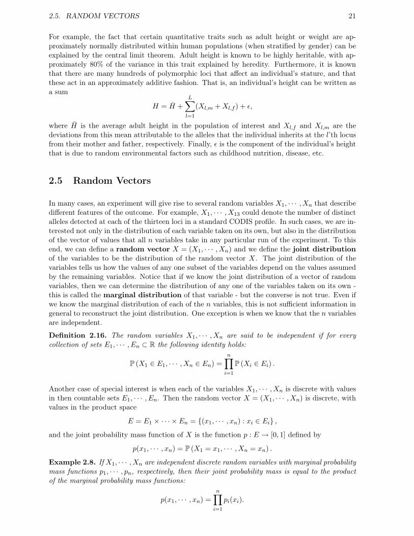
For example, the fact that certain quantitative traits such as adult height or weight are ap-proximately normally distributed within human populations (when stratified by gender) can beexplained by the central limit theorem. Adult height is known to be highly heritable, with ap-proximately 80% of the variance in this trait explained by heredity. Furthermore, it is knownthat there are many hundreds of polymorphic loci that affect an individual’s stature, and thatthese act in an approximately additive fashion. That is, an individual’s height can be written asa sum
H = H +L∑l=1
(Xl,m +Xl,f ) + ε,
where H is the average adult height in the population of interest and Xl,f and Xl,m are thedeviations from this mean attributable to the alleles that the individual inherits at the l’th locusfrom their mother and father, respectively. Finally, ε is the component of the individual’s heightthat is due to random environmental factors such as childhood nutrition, disease, etc.
2.5 Random Vectors
In many cases, an experiment will give rise to several random variables X1, · · · , Xn that describedifferent features of the outcome. For example, X1, · · · , X13 could denote the number of distinctalleles detected at each of the thirteen loci in a standard CODIS profile. In such cases, we are in-terested not only in the distribution of each variable taken on its own, but also in the distributionof the vector of values that all n variables take in any particular run of the experiment. To thisend, we can define a random vector X = (X1, · · · , Xn) and we define the joint distributionof the variables to be the distribution of the random vector X. The joint distribution of thevariables tells us how the values of any one subset of the variables depend on the values assumedby the remaining variables. Notice that if we know the joint distribution of a vector of randomvariables, then we can determine the distribution of any one of the variables taken on its own -this is called the marginal distribution of that variable - but the converse is not true. Even ifwe know the marginal distribution of each of the n variables, this is not sufficient information ingeneral to reconstruct the joint distribution. One exception is when we know that the n variablesare independent.
Definition 2.16. The random variables X1, · · · , Xn are said to be independent if for everycollection of sets E1, · · · , En ⊂ R the following identity holds:
P (X1 ∈ E1, · · · , Xn ∈ En) =n∏i=1
P (Xi ∈ Ei) .
Another case of special interest is when each of the variables X1, · · · , Xn is discrete with valuesin then countable sets E1, · · · , En. Then the random vector X = (X1, · · · , Xn) is discrete, withvalues in the product space
E = E1 × · · · × En = (x1, · · · , xn) : xi ∈ Ei ,
and the joint probability mass function of X is the function p : E → [0, 1] defined by
p(x1, · · · , xn) = P (X1 = x1, · · · , Xn = xn) .
Example 2.8. If X1, · · · , Xn are independent discrete random variables with marginal probabilitymass functions p1, · · · , pn, respectively, then their joint probability mass is equal to the productof the marginal probability mass functions:
p(x1, · · · , xn) =n∏i=1
pi(xi).

22 CHAPTER 2. PROBABILITY THEORY
The multinomial distribution is an example of a multivariate distribution for which the compo-nent variables are not independent.
Definition 2.17. A random vector (X1, · · · , Xm) is said to have the multinomial distributionwith parameters n ≥ 1 and (p1, · · · , pm) if X1, · · · , Xm take values in the set 0, · · · , n with jointprobability mass function
p(n1, · · · , nm) =(
n
n1, · · · , nm
) m∏i=1
pnii
provided that n1 + · · · + nm = n. Here p1, · · · , pm are non-negative numbers subject to thecondition p1 + · · ·+ pm = 1 and (
n
n1, · · · , nm
)=
n!n1! · · ·nm!
is the number of ways of choosing m subsets of sizes n1, · · · , nm from a set of n objects.
The multinomial distribution arises in the following setting. Suppose that n independent exper-iments are conducted and that each experiment can result in any one of m possible outcomes.If the probability that an experiment results in the i’th outcome is pi and Xi denotes the to-tal number of experiments with this outcome, then the random vector (X1, · · · , Xm) has themultinomial distribution with parameters n and (p1, · · · , pm).

Chapter 3
Topics in Population Genetics
3.1 Hardy-Weinberg Equilibrium
Suppose that k alleles A1, · · · , An are segregating at an autosomal locus. Then there are k(k +1)/2 distinct diploid genotypes: k homozygous genotypes AiAi and
(k2
)= k(k−1)
2 heterozygousgenotypes AiAj . (Recall that the order in which we write the two alleles in a heterozygousgenotype usually does not matter.) A basic question of interest in population genetics is howthe frequencies of the diploid genotypes relate to the frequencies of the alleles. The answer, ofcourse, depends on the biological details of the system, but a result known as Hardy-Weinbergequilibrium seems to hold, at least approximately, at many loci.
To derive the Hardy-Weinberg equilibrium, we will make the following assumptions:
• the population is infinite and has non-overlapping generations;
• the population is panmictic and random mating, so that mate choice is independent ofan individual’s genotype;
• the locus is selectively neutral, i.e., an individual’s genotype does not affect the proba-bility that they survive and reproduce or the number of offspring that they leave;
• segregation during meiosis adheres to Mendel’s first law, i.e., there is no meiotic drive;
• there is no mutation at the locus.
Let pij denote the frequency of AiAj heterozygotes in the current generation and let
pi = pii +12
∑j 6=i
pij
be the corresponding frequency of the allele Ai. Under the above assumptions, the frequency ofthe genotype AiAj in the next generation is equal to
p′ij =p2i if j = i
2pipj if j 6= i.(3.1)
Although this observation is the one that is most often associated with the phrase Hardy-Weinberg equilibrium, there is another equally important point, which is that the frequencyof allele Ai following one round of random mating is
p′i = p′ii +12
∑j 6=i
p′ij
23

24 CHAPTER 3. TOPICS IN POPULATION GENETICS
= p2i +
12
∑j 6=i
2pipj
= pi
k∑j=1
pj
= pi,
where the final identity follows from the fact that the sum of the frequencies of all k allelesis equal to 1. In other words, under the above assumptions, the frequencies of the alleles areconstant across generations and the frequencies of the diploid genotypes are constant after asingle round of random mating, no matter what the initial frequencies are.
There are many factors that can cause genotype frequencies to deviate from the values expectedunder Hardy-Weinberg equilibrium (HWE) and arguably the most important of these (at leastin the context of forensic genetics) is population structure. We will examine the consequencesof non-random mating being in a later section, but we first consider two statistical proceduresthat can be used to test whether the genotype counts in a random sample of individuals drawnfrom a population are consistent with the hypothesis that that locus is at HWE. A statisticaltest is necessary because even if HWE holds exactly in the population, it probably won’t holdin a random sample of individuals from the population.
3.1.1 Pearson’s Goodness-of-Fit Test
Suppose that n individuals are sampled from a population and let nij be the number of individualsin the sample with genotype Aij . Then we can estimate the genotype and allele frequencies as
pij =nijn
pi =1
2n
2nii +∑j 6=i
nij
,
where the hat over the variable indicates that it is an estimate rather than the true value.Furthermore, if HWE holds in the population and we define
Eij =np2
i if j = i2npipj if j 6= i,
(3.2)
then in a sufficiently large sample we would expect each of the differences
nii − Eij
between the observed and the expected numbers of Aij individuals in the sample to be small.Here I have put hats over the numbers Eij to indicate that these are only estimates of theexpected counts since these depend on our estimates of the allele frequencies. To test whetherthese differences are sufficiently small, we calculate the following goodness-of-fit test statistic
T =∑i≤j
(nij − Eij
)2Eij
and compare the observed value of T with the distribution of values that would be expectedunder HWE. Since the exact distribution is complicated, it is customary to instead use a largesample approximation based on the central limit theorem. For this particular problem, itcan be shown that in the limit of infinite sample size, the distribution of T is asymptotic to aχ2-distribution with k(k− 1)/2 degrees of freedom. A χ2-distribution with d degrees of freedom

3.1. HARDY-WEINBERG EQUILIBRIUM 25
is defined to be the distribution of the sum of the squares of d independent standard normalrandom variables. For our problem, the number of degrees of freedom is determined by notingthat there are k(k + 1)/2 different genotypes and that we lose one degree of freedom since thesum of these frequencies is 1 and we lose an additional k − 1 degrees of freedom by using thesample to estimate the allele frequencies, giving
d =k(k + 1)
2− 1− (k − 1) =
k(k − 1)2
as the total number of degrees of freedom for this test. To carry out this test in R, enter thefollowing command
> 1 - pchisq(T, df = d)
where T is the value of the test statistic and d is the number of degrees of freedom. Sincepchisq(q, df) gives the cumulative probability of values less than or equal to q, we need tosubtract this probability from 1 to calculate the probability of obtaining a test statistic as largeas or greater than the observed statistic.
A rule of thumb for the use of the χ2-distribution is that most of the counts nij should be at leastas large as 5 and none should be smaller than 2. When some of these counts are too small, thecentral limit theorem will not apply to the corresponding terms in T and then the χ2-distributionmay be too crude an approximation. In such cases, it is better to use the method described inthe next section.
3.1.2 Fisher’s Exact Test
If the number of alleles segregating at a locus is large (as will generally be the case with the STRloci used in forensics and relatedness testing), then it is likely that some of the possible diploidgenotypes will be represented by very few individuals in the sample or even be missing altogether.When this is true, the large-sample asymptotics used to justify the use of the χ2-distributionmay not be sufficiently accurate and it is preferable to work with the exact sampling distributionof the test statistic. One way to do this is by using Fisher’s exact test, which can be describedexplicitly for a locus segregating two alleles, say A and a.
Suppose that we sample n individuals and that the counts of the three diploid genotypes AA, Aaand aa in this sample are nAA, nAa and naa, respectively. Then the number of A and a allelespresent in the sample are given by
nA = 2nAA + nAa and na = 2naa + nAa. (3.3)
Let the true (but unknown) allele frequencies be pA and pa = 1 − pA and assume that thegenotype frequencies in the population are in HWE. To carry out Fisher’s exact test, we beginby calculating the probability that a sample of n individuals contains the observed genotypecounts conditional on it containing nA A alleles and na a alleles:
P(nAA, nAa, naa|nA, na
)=P(nAA, nAa, naa
)P(nA, na
) (3.4)
provided that the allele counts and the genotype counts are consistent, i.e., equation (3.3) holds.Since the number of A alleles in a sample containing n individuals from a population in whichthe frequency of A is pA is binomially distributed with parameters 2n and pA, it follows that theprobability in the denominator is given by
P(nA, na
)=(
2nnA
)pnAA pna
a =(2n)!nA!na!
pnAA pna
a

26 CHAPTER 3. TOPICS IN POPULATION GENETICS
whenever 2n = nA + na. Similarly, since the vector of genotype counts (nAA, nAa, naa) is multi-nomially distributed with parameters n and (pAA, pAa, paa), it follows that the probability in thenumerator is
P(nAA, nAa, naa
)=
(n
nAA, nAa, naa
)pnAaAA p
naaaa
=n!
nAA!nAa!naa!p2nAAA (2pApa)nAap2na
a
=n!
nAA!nAa!naa!2nAapnA
A pnaa ,
where the identity of the first and second lines is a consequence of HWE and the identity ofthe second and third lines is a consequence of equation (3.3). Upon substituting these resultsinto equation (3.4), the terms involving the allele frequencies cancel and we obtain the followingprobability
P(nAA, nAa, naa|nA, na
)=
2nAan!nA!na!(2n)!nAA!nAa!naa!
. (3.5)
The p-value for Fisher’s exact test is then calculated by summing the conditional probabilitiesof all possible outcomes that are either as or less probable than the observed outcome. Since theonly outcomes that are relevant are those which satisfy nA = 2xAA + xAa and na = 2xaa + xAa,this computation can be done by exhaustive enumeration.
Fisher’s exact test can also be extended to loci segregating more than two alleles. As in thebiallelic case, we first calculate the probability of the genotype counts conditional on the observednumbers of alleles
P(nAiAj , 1 ≤ i ≤ j ≤ k|nAi , 1 ≤ i ≤ k
)and then sum the conditional probabilities of all possible outcomes that are at least as unlikely asthe observed outcome. In practice, there may be too many possibilities to enumerate explicitlyand Monte Carlo techniques are used instead which sample from the set of possible outcomes.
3.1.3 The Inbreeding Coefficient
An alternative approach is to generalize the model underlying Hardy-Weinberg equilibrium byallowing inbreeding. Suppose that the assumptions listed at the beginning of this section aremodified so that with probability 1−f mating is random and with probability f a gamete uniteswith another gamete carrying the same allele. f is called the inbreeding coefficient and isa measure of the tendency of individuals to mate with other individuals who are more closelyrelated to themselves than to another random-chosen member of the population. If there aretwo alleles A and a segregating at the locus with frequencies pA and pa, then under inbreeding,the genotype frequencies after a single generation will be equal to
pAA = (1− f)p2A + fpA (3.6)
pAa = 2(1− f)pApa (3.7)paa = (1− f)p2
a + fpA. (3.8)
Notice that if f = 0, then there is no inbreeding and we are back to the conditions underlyingHWE, while if f = 1, then all individuals are completely inbred and only homozygotes willbe found in the population. Given a sample of n individuals in which the counts of the threegenotypes are nAA, nAa, and naa, the likelihood function L(pA; f) of the inbreeding coefficientf and the allele frequency pA is defined to be equal to the probability of the data under thoseparticular values of f and pA. (Notice that pA is determined by pA since the two frequencies
3.1. HARDY-WEINBERG EQUILIBRIUM 27
sum to 1.) Assuming that we have sampled from an infinite population, this probability is givenby the multinomial distribution with parameters n and (pAA, pAa, paa) and so
L(pA; f) ≡(
n
nAA, nAa, naa
)pnAAAA pnAa
Aa pnaaaa
=(
n
nAA, nAa, naa
)((1− f)p2
A + fpA)nAA (2(1− f)pApa)
nAa((1− f)p2
a + fpA)naa
.
If the allele frequency pA were known exactly, the inbreeding coefficient could be estimated fromthe data by finding the value of f that maximizes the likelihood of the data. This estimateis called the maximum likelihood estimate (MLE) of f . Although the MLE can be foundanalytically by solving a cubic equation, in practice the solution is found numerically usingNewton’s method or a similar algorithm. For the more realistic scenario in which the allelefrequencies are not known exactly, these can be jointly estimated along with the inbreedingcoefficient by maximizing the likelihood function with respect to both unknown parameters. Inthis case, the estimates can only be found numerically.
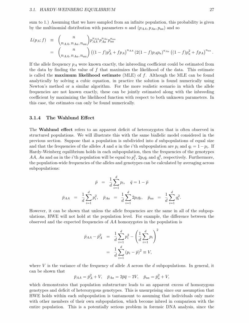
3.1.4 The Wahlund Effect
The Wahlund effect refers to an apparent deficit of heterozygotes that is often observed instructured populations. We will illustrate this with the same biallelic model considered in theprevious section. Suppose that a population is subdivided into d subpopulations of equal sizeand that the frequencies of the alleles A and a in the i’th subpopulation are pi and qi = 1−pi. IfHardy-Weinberg equilibrium holds in each subpopulation, then the frequencies of the genotypesAA, Aa and aa in the i’th population will be equal to p2
i , 2piqi and q2i , respectively. Furthermore,the population-wide frequencies of the alleles and genotypes can be calculated by averaging acrosssubpopulations:
p =1d
d∑i=1
pi, q = 1− p
pAA =1d
d∑i=1
p2i , pAa =
1d
d∑i=1
2piqi, paa =1d
d∑i=1
q2i .
However, it can be shown that unless the allele frequencies are the same in all of the subpop-ulations, HWE will not hold at the population level. For example, the difference between theobserved and the expected frequencies of AA homozygotes in the population is
pAA − p2A =
1d
d∑i=1
p2i −
(1d
d∑i=1
pi
)2
=1d
d∑i=1
(pi − p)2 ≡ V,
where V is the variance of the frequency of allele A across the d subpopulations. In general, itcan be shown that
pAA = p2A + V, pAa = 2pq − 2V, paa = p2
a + V,
which demonstrates that population substructure leads to an apparent excess of homozygousgenotypes and deficit of heterozygous genotypes. This is unsurprising since our assumption thatHWE holds within each subpopulation is tantamount to assuming that individuals only matewith other members of their own subpopulation, which become inbred in comparison with theentire population. This is a potentially serious problem in forensic DNA analysis, since the

28 CHAPTER 3. TOPICS IN POPULATION GENETICS
presence of population structure in human populations means that we cannot simply assumeHWE when calculating match probabilities at diploid loci. Furthermore, although geographicalseparation is an important source of population structure (mating is more more likely to occurbetween individuals that live in the same region), structure can also arise from less evident factorssuch as ethnicity, religion, race, etc. Of course, the model described in this section is somewhatunrealistic in that it assumes that the subpopulations are completely reproductively isolated,but heterozygote deficiency will also occur when there is gene flow between the subpopulations.
3.2 Genetic Drift
Although one of the predictions of Hardy-Weinberg equilibrium is that allele frequencies areconstant across generations, we would only expect this to hold approximately in a real populationand then only over relatively short time scales. In fact, there are multiple processes that can causeallele frequencies to change, sometimes rapidly, including genetic drift, mutation, migration, andselection.
Recall that one of our assumptions in the section on HWE was that the population is infinite.This allowed us to equate sampling probabilities with frequencies and meant that we couldpredict the exact frequencies of the genotypes in each generation. However, because individualsurvival, reproduction and mating all depend to some extent on sequences of chance events, thefrequency of an allele or genotype in a finite population will fluctuate between generations. Forexample, if the population contains only two haploid individuals with genotypes A and a andby chance the second individual dies before reproducing, then only A alleles will be present inthe next generation and so the frequency of this allele will have increased from 0.5 to 1. Thisprocess of random fluctuations in allele frequencies is known as genetic drift.
Stochastic models have played an important role in studies of genetic drift and its evolutionaryconsequences and here we consider one of the best known of these models. The Wright-Fishermodel is a discrete-time Markov chain that was introduced by Sewall Wright and R. A. Fisherin the 1930’s. It makes the following assumptions:
• The population is of constant size N and has non-overlapping generations.
• Each individual alive in generation t+ 1 ‘chooses’ its parent uniformly at random and withreplacement from among the N individuals alive in generation t.
• We consider a haploid locus segregating neutral alleles A and a.
• There is no mutation and each individual inherits their parent’s genotype.
If pt denotes the frequency of allele A in generation t, then the conditional distribution of Npt+1
given pt = p is binomial with parameters N and p, i.e., there are N individuals and the genotypeof each one is determined by randomly choosing one of the N individuals alive in the previousgeneration, which will have genotype A with probability p and genotype a with probability 1−p.It follows that the expected frequency of A in generation t+ 1 is the same as the frequency of Ain the preceding generation,
E[pt+1|pt = p] = p,
and so genetic drift leaves the expected values of the allele frequencies unchanged. On the otherhand, pt+1 is a random quantity which need not be equal to p and the conditional variance ofpt+1 given pt = p is
Var (pt+1|pt = p) =p(1− p)N
.
3.2. GENETIC DRIFT 29
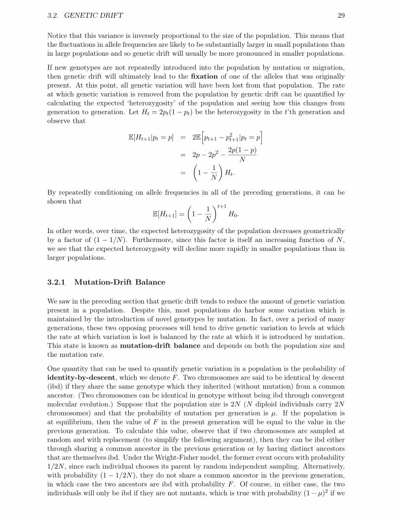
Notice that this variance is inversely proportional to the size of the population. This means thatthe fluctuations in allele frequencies are likely to be substantially larger in small populations thanin large populations and so genetic drift will usually be more pronounced in smaller populations.
If new genotypes are not repeatedly introduced into the population by mutation or migration,then genetic drift will ultimately lead to the fixation of one of the alleles that was originallypresent. At this point, all genetic variation will have been lost from that population. The rateat which genetic variation is removed from the population by genetic drift can be quantified bycalculating the expected ‘heterozygosity’ of the population and seeing how this changes fromgeneration to generation. Let Ht = 2pt(1− pt) be the heterozygosity in the t’th generation andobserve that
E[Ht+1|pt = p] = 2E[pt+1 − p2
t+1|pt = p]
= 2p− 2p2 − 2p(1− p)N
=(
1− 1N
)Ht.
By repeatedly conditioning on allele frequencies in all of the preceding generations, it can beshown that
E[Ht+1] =(
1− 1N
)t+1
H0.
In other words, over time, the expected heterozygosity of the population decreases geometricallyby a factor of (1 − 1/N). Furthermore, since this factor is itself an increasing function of N ,we see that the expected heterozygosity will decline more rapidly in smaller populations than inlarger populations.
3.2.1 Mutation-Drift Balance
We saw in the preceding section that genetic drift tends to reduce the amount of genetic variationpresent in a population. Despite this, most populations do harbor some variation which ismaintained by the introduction of novel genotypes by mutation. In fact, over a period of manygenerations, these two opposing processes will tend to drive genetic variation to levels at whichthe rate at which variation is lost is balanced by the rate at which it is introduced by mutation.This state is known as mutation-drift balance and depends on both the population size andthe mutation rate.
One quantity that can be used to quantify genetic variation in a population is the probability ofidentity-by-descent, which we denote F . Two chromosomes are said to be identical by descent(ibd) if they share the same genotype which they inherited (without mutation) from a commonancestor. (Two chromosomes can be identical in genotype without being ibd through convergentmolecular evolution.) Suppose that the population size is 2N (N diploid individuals carry 2Nchromosomes) and that the probability of mutation per generation is µ. If the population isat equilibrium, then the value of F in the present generation will be equal to the value in theprevious generation. To calculate this value, observe that if two chromosomes are sampled atrandom and with replacement (to simplify the following argument), then they can be ibd eitherthrough sharing a common ancestor in the previous generation or by having distinct ancestorsthat are themselves ibd. Under the Wright-Fisher model, the former event occurs with probability1/2N , since each individual chooses its parent by random independent sampling. Alternatively,with probability (1 − 1/2N), they do not share a common ancestor in the previous generation,in which case the two ancestors are ibd with probability F . Of course, in either case, the twoindividuals will only be ibd if they are not mutants, which is true with probability (1−µ)2 if we

30 CHAPTER 3. TOPICS IN POPULATION GENETICS
assume that different lineages mutate independent. This leads to the following identity
F =
12N
+(
1− 12N
)F
(1− µ)2,
which can then be solved for F, giving
F =1
2N1
2N − 1 + 1(1−µ)2
≈ 11 + 4Nµ
(3.9)
where the latter approximation is valid if µ 1 (as is usually the case). Equation (3.9) showsthat the probability of identity-by-descent in a population will be small if the product 4Nµ islarge, which in turn will be true whenever genetic drift is weak relative to mutation.
It is also possible to derive the stationary distribution of allele frequencies for some finite popu-lation models with mutation. If the Wright-Fisher model is modified so that allele A mutates toa with probability ν and a mutates to A with probability µ, then the stationary distribution ofthe frequency p of allele A can be approximated by the Beta distribution with density
π(p) =1
β(4Nµ, 4Nν)p4Nµ−1(1− p)4Nν−1.
The normalizing constant β(a, b) in this expression is the Beta function defined by
β(a, b) ≡∫ 1
0xa−1(1− x)b−1dx.
This density is bimodal when 4Nµ, 4Nν 1, in which case mutation is much weaker thangenetic drift and the frequency of A will usually be either very close to 1 or very close to 0,i.e., most of the time, one of the two alleles will be close to being fixed in the population. Byexploiting certain properties of the Beta function, it can be shown that the average frequency ofA and the average heterozygosity in a population at equilibrium are given by
E[p] =µ
µ+ ν
E[2p(1− p)] =2µν
(µ+ ν)(µ+ ν + 14N )
.
Whereas the mean frequency of A is independent of the population size, we see that the expectedheterozygosity is an increasing function of N . This result is unsurprising since genetic drift isweaker in larger populations, which in turn means that larger population swill tend to retainmore genetic variation (i.e., higher heterozygosity) than smaller populations.
3.2.2 Population Structure
Although stochastic models of structured populations are very complicated, a great deal hasbeen learned about the effects of population structure on genetic variation and differentiationfrom the study of several highly simplified models. One of these is known as Wright’s islandmodel, which makes the following assumptions:
• The population is subdivided into a large number D of subpopulations.
• Each subpopulation is of constant size and contains N diploid individuals.
• Mating is random within subpopulations, but each offspring migrates to a new subpopula-tion with probability m.

3.2. GENETIC DRIFT 31
• The newborn individual replaces one of the N individuals alive in the subpopulation whereit settles.
Here m can be interpreted as a migration or dispersal rate: when m = 0, the subpopulations arecompletely isolated, while if m = 1, then the population is effectively panmictic.
Because each subpopulation is much smaller than the population as a whole, genetic drift has amuch stronger impact on the allele frequencies within subpopulations than on the global allelefrequencies. In particular, the subpopulation allele frequencies fluctuate more rapidly than do theglobal allele frequencies which therefore we treat as constant. (This phenomenon of having bothrapidly and slowly varying quantities in the same model is known as separation-of-timescales.)Suppose that there are K alleles, A1, · · · , AK , with global allele frequencies p1, · · · , pK thatsum to 1. Then it can be shown that the equilibrium distribution of allele frequencies within asubpopulation can be approximated by the Dirichlet distribution with density
π(x1, · · · , xK |p1, · · · , pK) =Γ(λ)∏K
k=1 Γ(λpk)
K∏k=1
xλpk−1k (3.10)
where
Γ(c) =∫ ∞
0xc−1e−xdx (Gamma function)
λ =1θ− 1 = 4Nm.
When K = 2, this distribution is just the Beta distribution introduced in the previous section,albeit with different parameters.
The coefficient θ is usually denoted FST in the population genetics literature and measures thedegree of genetic differentiation between the subpopulations. When θ ≈ 0, the subpopulations areessentially undifferentiated and the local allele frequencies deviate from the global frequenciesvery little. In contrast, when θ ≈ 1, then the subpopulations are highly differentiated andtypically only one of the K alleles will be present in each subpopulation. For the island modeldescribed above, the equilibrium value of θ is equal to
θ =1
1 + 4Nm,
which will be small whenever the product 4Nm is large. This is reminiscent of the result forthe equilibrium probability of ibd in a model with genetic drift and mutation, except that in thepresent scenario it is migration rather than mutation that is responsible for introducing geneticvariation into a subpopulation. Most estimates of θ for human populations lie between 0 and0.05, indicating that these populations are only weakly genetically differentiated, either becausethey are of recent origin or because of ongoing gene flow.
3.2.3 Sampling Distributions
Suppose that n chromosomes are sampled at random from a population and typed at a diploidlocus at which K distinct alleles A1, · · · , AK have been identified. If the frequencies of thesealleles are known, say p1, · · · , pK , then the the probability that our sample contains n1 copiesof A1, n2 copies of A2, and so forth, is given by the multinomial distribution with parameters nand (p1, · · · , pK):
p(n1, · · · , nK |p1, · · · , pK) =(
n
n1, · · · , nK
) K∏k=1
pnkk . (3.11)

32 CHAPTER 3. TOPICS IN POPULATION GENETICS
This expression assumes that sampling is completely random with respect to any latent structurein the population, i.e., the probability that a particular group of chromosomes is sampled isindependent of their membership in any genetically-differentiated subpopulations. In particular,if the sample is obtained by sampling individuals at random and typing both of the chromosomesthat these individuals carry, then the multinomial distribution will only be appropriate when thepopulation is at Hardy-Weinberg equilibrium. However, as we saw in Section 3.1.4, HWE usuallywill not hold in the population as a whole when there are subpopulations with different allelefrequencies.
In some cases, this problem can be addressed with the help of the island model described inthe previous section. Suppose that the population is subdivided into a large number of demesand that the unknown allele frequencies in each deme are distributed according to the Dirichletdistribution shown in Equation (3.10). Recall that (3.10) depends on the global allele frequen-cies, p1, · · · , pK , which we assume are known. If these assumptions hold, then we can derivethe sampling distribution of a group of chromosomes sampled from the same subpopulation byaveraging the multinomial probability shown in (3.11) over the distribution of the unknown al-lele frequencies in that deme. To do so, we will need to integrate over the (K − 1)-dimensionalsimplex DK = (x1, · · · , xK) : x1, · · · , xK ≥ 0, x1 + · · ·+ xK = 1 and we obtain
ps(n1, · · · , nK) =∫DK
p(n1, · · · , nK |x1, · · · , xK)π(x1, · · · , xK |p1, · · · , pK)dx1 · · · dxK
=∫DK
(n
n1, · · · , nK
) K∏k=1
xnkk
Γ(λ)∏Ki=1 Γ(λpi)
K∏k=1
xλpk−1k dx1 · · · dxK
=(
n
n1, · · · , nK
)Γ(λ)∏K
k=1 Γ(λpk)
∫DK
K∏k=1
xnk+λpk−1k dx1 · · · dxK
=(
n
n1, · · · , nK
)Γ(λ)∏K
k=1 Γ(λpk)
∏Kk=1 Γ(λpk + nk)
Γ(λ+ n)
=(
n
n1, · · · , nK
)Γ(λ)
Γ(λ+ n)
K∏k=1
Γ(λpi + nk)Γ(λpk)
=(
n
n1, · · · , nK
)n−1∏j=0
1λ+ j
K∏k=1
nk−1∏j=0
(λpk + j)
,
where we have used the following two identities to pass from the third to the fourth and fromthe fifth to the sixth lines in the above:∫
DK
K∏k=1
xak−1k dx1 · · · dxK =
∏Kk=1 Γ(ak)
Γ(∑K
k=1 ak)
Γ(a+ n) = (a+ n− 1)Γ(a+ n− 1) for any a > 0.
The ‘s’ subscript is included in ps to remind us that this is the sampling distribution for asample from a structured population. We can also express this distribution in terms of thekinship coefficient θ by substituting 1
θ − 1 for λ in the last line:
ps(n1, · · · , nK) =(
n
n1, · · · , nK
)∏Kk=1
∏nk−1j=0 (jθ + (1− θ)pk)
(1− θ)∏n−2j=1 (1 + jθ)
. (3.12)
This is the probability of an unordered sample. In some instances, we will want to know theprobability of an ordered sample in which A1 appears n1 times, etc., and this is obtained by

3.2. GENETIC DRIFT 33
dividing (3.12) by the number of such ordered samples, which is given by the leading multinomialcoefficient in that expression:
ps;o(n1, · · · , nK) =
∏Kk=1
∏nk−1j=0 (jθ + (1− θ)pk)
(1− θ)∏n−2j=1 (1 + jθ)
. (3.13)
I have included an ‘o’ in the subscript of this probability to emphasize that it refers to an orderedsample. Caveat: Although Balding is careful to distinguish between ordered and unorderedsamples in his book, the two appear to be conflated in the discussion that appears on p. 39 ofFung & Hu (2008). In particular, equation (3.14) of the latter reference gives the probability ofan ordered sample and is not equal to the line that immediately precedes it (which applies to anunordered sample).
Example 3.1. If n = ni = 1, then the only non-empty product in the numerator will be thatcorresponding to k = i (empty products are set equal to 1 by convention) and we obtain
ps(Ai) =(1− θ)pi(1− θ)
= pi,
as expected since population structure does not change the sampling distribution of a single chro-mosome. If n = 2, then there are two possibilities. Suppose that both chromosomes carry Aialleles, i.e., n = ni = 2. Then
ps(Ai, Ai) =(1− θ)pi · (θ + (1− θ)pi)
(1− θ)= p2
i + θpi(1− pi).
Alternatively, if the sample contains one Ai allele and one Aj allele, where i 6= j, then
ps(Ai, Aj) = 2(1− θ)pi · (1− θ)pj
(1− θ)= 2(1− θ)pipj ,
where the factor of 2 accounts for the fact that the two alleles could be sampled in either order.Notice that when θ = 0, these sampling probabilities are identical to those derived under HWE.However, when θ > 0, there will be an excess of homozygous samples and a deficit of heterozygoussamples, in accordance with the Wahlund effect.
Conditional Sampling Probabilities
One reason for writing down the ordered sample probability in (3.13) is so that we can useit to calculate the conditional distribution of alleles in future samples of chromosomes from apopulation that has already been sampled. For example, suppose that we previously sampledn chromosomes from a population and that n1 of these were A1 alleles, n2 were A2 alleles, etc.Then the conditional probability that the next chromosome sampled from the population willcarry an Ai allele equal to
ps,o(n1, · · · , ni + 1, · · · , nK)ps,o(n1, · · · , ni, · · · , nK)
=niθ + (1− θ)pinθ + (1− θ)
. (3.14)
Notice that this expression depends only on the number of Ai alleles in the original sample andon the size of that sample. For example, if we have previously sampled an A1A1 homozygotefrom a population, then the conditional distribution of the allele carried by a third chromosomethat is sampled from the same population will be
P(A1|A1A1) =2θ + (1− θ)p1
2θ + (1− θ)≥ p1

34 CHAPTER 3. TOPICS IN POPULATION GENETICS
P(A2|A1A1) =(1− θ)p2
2θ + (1− θ)≤ p2,
and we will have strict inequalities on the right-hand side whenever θ > 0. In other words,each time that we sample a given allele from a structured population, the chances of observingadditional copies of that allele in future samples increase. The reason for this is that our initialsample is informative about the unknown frequencies of alleles in that particular subpopulationand our (posterior) estimates of these frequencies will either increase or decrease depending onwhether the alleles are present in or absent from our original sample.
3.2.4 Linkage Equilibrium
A set of polymorphic loci is said to be in linkage equilibrium if the allelic states of the locion a randomly sampled gamete are independent. For example, if there are n alleles A1, · · · , Ansegregating at the first locus with frequencies pA1 , · · · , pAn and m alleles B1, · · · , Bm segregat-ing at the second locus with frequencies pB1 , · · · , qBm , then the population will be at linkageequilibrium if the frequency of the two-locus gamete with alleles AiBj is
pAiBj = pAipBj
for each 1 ≤ i ≤ n and 1 ≤ j ≤ m. If n = m = 2, then it suffices to check just one of theseidentities, say
pA1B1 = pA1pB1 ,
as this will imply that the other three identities hold as well.
One prediction of Mendel’s second law is that linkage equilibrium will hold at any set of neutralunlinked loci (e.g., loci located on different chromosomes) in an infinite randomly-mating pop-ulation. In practice, these conditions never hold exactly and several factors, including physicallinkage, genetic drift, population structure and selection, can create associations between thealleles found at different loci on the same gamete, a state known as linkage disequilibrium. Fora two-locus, two-allele system, the strength of these associations can be quantified by a singlestatistic which is usually either the covariance between two of the allele frequencies
D = pA1B1 − pA1pB1
or the correlation coefficientr =
D√pA1pA2pB1pB2
.
Notice that D = r = 0 under linkage equilibrium and that positive values of D (or r) indicatethat the alleles A1 and B1 occur together on the same gamete disproportionately often. Severalmethods, including Pearson’s goodness-of-fit test and Fisher’s exact test, have been developedthat can be used to test for linkage equilibrium using samples of either haploid or (unphased)diploid genotypes. Although weak deviations can be found for some of the CODIS core STRloci, these are thought to mainly be due to population structure and are handled by using thesampling formula corrections described in the preceding section.

Chapter 4
DNA Profiling
4.1 Match Probabilities
The main statistical issue that must be addressed in genetic profiling is the following. Supposethat some DNA is recovered from a crime scene and is found to have the same genotype G as asample of DNA collected from a known individual S. How strong is the evidence that S is alsothe source of the first sample? To address this question, we can set up a hypothesis test withthe following hypotheses:
HS : S is the source of the DNA in the first sample;HI : a different individual I is the source of the first sample.
Notice that the evidence E includes two pieces of information: that the source of the sample hasgenotype G and that individual S also has genotype G. We can assess the relative support thatthe evidence provides for these two hypotheses by calculating the following likelihood ratio
L ≡ P(E|HS)P(E|HI)
.
In general, the larger the likelihood ratio L is, the stronger the evidence is in favor of HS ratherthan HI . If we assume that no errors have been made during the handling and genotyping ofthe data, then we can show that the reciprocal of the likelihood ratio is equal to the matchprobability of a random individual I to the profile G, conditional on the observation that Salso has this profile:
RI ≡ L−1 =P(I and S both have genotype G)
P(S has genotype G)= P
(I has genotype G|S has genotype G
).
To make further progress, we need to be more specific about the genetic profile G and thepopulation genetics of the relevant populations. Let us begin by considering a single diploidlocus segregating alleles A1, · · · , AK at frequencies p1, · · · , pK and assume that S, I and theunknown source of the sample all come from the same population, which is at Hardy-Weinbergequilibrium. If S and I are unrelated, then the genotypes of S and I are independent and thematch probability is just the unconditional probability that I has genotype G = AiAj :
RI =p2i if j = i
2pipj if j 6= i,
As expected, rarer genotypes G provide stronger evidence in favor of HS .
35

36 CHAPTER 4. DNA PROFILING
Next, suppose that HWE is violated because of the presence of population structure. If we haveno reason to believe that S and I belong to the same subpopulation, then we can continue toassume that the two are unrelated and therefore that their genotypes are independent. In theabsence of specific information concerning the allele frequencies in the subpopulations, we canuse the sampling distribution derived for the island model in Section 3.2.3 to calculate the matchprobability for I to genotype G:
RI =
(1− θ)p2i + θpi if j = i
2(1− θ)pipj if j 6= i,
where θ is the inbreeding coefficient. Since θ typically lies between 0 and 0.05 for large humanpopulations, this correction will have only a very small impact on the likelihood ratio L when thesample genotype G is heterozygous. On the other hand, if the sample genotype is homozygous,say G = AiAi, and the global frequency of the allele Ai is of the same order as θ, then inbreedingcould reduce the likelihood ratio by a factor of two or more relative to the value calculatedassuming HWE. In fact, since these expressions are based on a very crude model of humanpopulation structure and depend on a parameter θ that can only be estimated, the secondNational Research Council report (NRC II, 1996) recommended that match probabilities becalculated using the following formulas
RI =
(1− θ)p2i + θpi if j = i
2pipj if j 6= i.
These can be said to be conservative with respect to the hypothesis HS in the sense that theyprobably underestimate the evidence in favor of HS and thus would give a defendant the ‘benefitof the doubt’ in a criminal case.
If S and I belong to the same subpopulation, then the two will be more likely to share the samegenotype than two individuals sampled at random from the population as a whole. In this case,the match probability can be calculated with the help of the conditional sampling distributionshown in Equation (3.14). First consider the case where G = AiAi is homozygous. Then thematch probability is the same as the conditional probability that two additional Ai alleles aresampled given that two have already been sampled:
RI = P(AiAi|AiAi)= P(Ai|AiAi) · P(Ai|AiAiAi)
=(
2θ + (1− θ)pi1 + θ
)(3θ + (1− θ)pi
1 + 2θ
)=
(2θ + (1− θ)pi)(3θ + (1− θ)pi)(1 + θ)(1 + 2θ)
.
If instead the sample genotype G = AiAj is heterozygous, then we need to multiply the condi-tional sampling probability by a factor of two to account for the two different orders in whichthe two alleles of I could be sampled (this does not matter for S since the factor of 2 wouldappear in both the numerator and denominator of the match probability and thus will cancel).Repeated application of (3.14) here gives:
RI = 2 · P(AiAj |AiAj)= 2 · P(Ai|AiAj) · P(Aj |AiAiAj)
= 2 ·(θ + (1− θ)pi
1 + θ
)(θ + (1− θ)pj
1 + 2θ
)= 2 · (θ + (1− θ)pi)(θ + (1− θ)pj)
(1 + θ)(1 + 2θ).

4.1. MATCH PROBABILITIES 37
As a general rule, the match probabilities for homozygous genotypes are always increasing func-tions of θ, whereas the match probabilities for heterozygous genotypes can be either increasingor decreasing depending on the global allele frequencies. This is because inbreeding has two op-posing effects on the conditional probability that a second individual is also a heterozygote. Onthe one hand, inbreeding reduces heterozygosity since individuals are disproportionately likelyto inherit alleles that are identical-by-descent. On the other hand, if the global frequencies ofAi and Aj are small, then observing an individual with genotype AiAj in a subpopulation hasthe effect of shifting the conditional distribution of the local frequencies of the two alleles in thatsubpopulation to larger values, and this effect becomes stronger as θ increases. Since forensicmarkers are usually deliberately chosen so that the frequencies of the alleles are small (and there-fore more informative about identity), the match probabilities for both kinds of genotypes areexpected to be increasing functions of θ in practice.
4.1.1 Power of Discrimination
Although there are many polymorphic loci within the human genome, these are not all equallyuseful for the purposes of identification. One statistic that is sometimes used to evaluate thesuitability of different loci for DNA profiling is the power of discrimination (PD), which is justthe probability that two individuals, say X and Y , chosen at random have different genotypes atthat locus. For example, the power of discrimination at a locus segregating K alleles A1, · · · , AKwith frequencies p1, · · · , pK in a population that is panmictic and at Hardy-Weinberg equilibriumis equal to
PD = 1−∑i≤jP(X = AiAj , Y = AiAj)
= 1−∑i≤jP(X = AiAj)2
= 1−
K∑i=1
p4i + 4
∑i<j
p2i p
2j
.
In general, the power of discrimination will be greatest at loci segregating many alleles at ap-proximately equal frequencies.
4.1.2 Multiple Loci
Suppose that S is typed at several loci and found to have alleles A(l)i A
(l)j at the l’th locus, where
1 ≤ l ≤ L. If the loci are in linkage equilibrium (cf. section 3.2.4), then the match probability ofan individual I to the multilocus genotype G can be calculated using the product rule
RI(G) =L∏l=1
R(l)I ,
where R(l)I is the single locus match probability at locus l given by one of the formulas derived
above. This rule is expected to give a good approximation to the true match probability whenthe population is large and panmictic and when the different loci are unlinked, e.g., on differentchromosomes, and evolve neutrally. Unfortunately, although three out of four of these conditionsare more or less satisfied by the core STR loci used in forensic work, the fact that humanpopulations are not panmictic is thought to be responsible for the modest levels of linkagedisequilibrium (LD) that have been documented between some of these loci. This matters in

38 CHAPTER 4. DNA PROFILING
DNA profiling because one of the consequences of LD is to cause the match probabilities forcommon multi-locus genotypes to be underestimated when the product rule is applied to singlelocus match probabilities based on global allele frequencies. This can then lead to overestimatesof the strength of the evidence indicating that a suspect S is the true source of a sample ofDNA. Although one could correct for this bias by formulating a multi-locus extension of theisland model, a simpler solution is to apply the product rule to one-locus match probabilitiesthat have been calculated using overestimates of the inbreeding coefficient θ. For example, ifthe ‘true’ value of θ is estimated to be approximately 0.01, one takes θ = 0.02 when computingR
(l)I and then multiplies these match probabilities together. Balding (2005) suggests that this
approach probably overestimates the multi-locus match probabilities and therefore errs in favorof the suspect S.
When the product rule holds, the power of discrimination for a set of loci can be calculated usingthe formula
PD = 1−L∏l=1
(1− PDl)
where PDl is the probability of discrimination at the l’th locus in the set. For example, ifPDl = 0.9 for each l = 1, · · · , 13 (a typical value for the core CODIS STR loci), then the powerof discrimination for the complete 13-locus genotype is
PD = 1−(
1− 910
)13
= 1−×10−13.
Of course, the actual match probabilities for specific genotypes can be substantially larger orsmaller than the difference 1− PD, so the probability of discrimination only measures how wellthe set of markers performs on average.
4.2 Relatives
To calculate the match probability when I is a close relative of S, let Z be the number of allelesthat are identical by descent (ibd) in I and S at the typed locus and define the relatednesscoefficients (k0, 2k1, k2) as
k0 = P(Z = 0)2k1 = P(Z = 1)k2 = P(Z = 2).
For example, in the absence of inbreeding, a parent and child will share exactly one allele thatis ibd and so k0 = k2 = 0 and 2k1 = 1. Similarly, if I and S are full sibs and their parentsare unrelated, then repeated application of Mendel’s first law shows that k0 = k2 = 1/4 and2k1 = 1/2. In general, the more closely related two individuals are, the larger will be the valuesof k1 and k2. In fact, we can combine the relatedness coefficients into a single number F , knownas the kinship coefficient, that is a simple measure of the genetic relatedness of two individuals.F is defined to be the probability that two alleles, one sampled at random from each individualI and S, are identical by descent. Furthermore, it can be shown that F is the average of k1 andk2:
F =12
(k1 + k2) .
Caveat: Unfortunately, Balding (2005) and Fung & Hu (2008) use different conventions in theirdiscussions of relatedness. My discussion follows section 3.6 of the latter reference because I willneed it for material that we will cover later in the course, but I actually prefer Balding’s notation

4.3. ADDITIONAL EVIDENCE 39
(section 6.2.4) which defines probabilities κt = P(Z = t) for t = 0, 1, 2. For comparison, noticethat κ0 = k0, κ2 = k2 and κ1 = 2k1.
By conditioning on the number of alleles that are ibd between I and S and using the law of totalprobability, the match probability of I to G can be written as
RI =2∑t=0
P(I = G|S = G, Z = t
)· P(Z = t)
≡ m0 · k0 +m1 · (2k1) +m2 · k2,
where mt is the match probability for I to G when I and S share t alleles that are ibd at thatlocus. Notice that mt depends on G, whereas kt does not. If t = 2, then I and S necessarilyhave the same genotype at that locus and so the conditional match probability is just m2 = 1. Ift = 0, then I and S share no alleles at the locus that are ibd, which means that the probabilityof a match for I to G is the same as that for an individual that is randomly chosen from thepopulation (or subpopulation) and so m0 can be calculated using the most appropriate formulafrom the preceding section. The case t = 1 is somewhat more complicated. If the genotypeG = AiAi is homozygous, then I will necessarily have at least one Ai allele which is identical bydescent to one of those carried by S and so m1 is just the conditional probability that I has asecond Ai allele conditional on S having genotype G:
m1 = P(Ai|AiAi) =2θ + (1− θ)pi
1 + θG = AiAi
If, instead, S has the heterozygous genotype G = AiAj with j 6= i, then the allele that is identicalby descent in I and S is equally likely to be Ai or Aj . Taking these two possibilities into accountleads to the following expression for m1:
m1 =12· P(Ai|AiAj) +
12· P(Aj |AiAj)
=12
(θ + (1− θ)pi) + (θ + (1− θ)pj)1 + θ
=θ + (1− θ)(pi + pj)/2
1 + θG = AiAj .
Some explicit formulas for RI are given in Table 3.15 of Fung & Hu (2008) for different relation-ships between I and S.
4.3 Additional Evidence
Suppose that there is additional evidence E (favorable or unfavorable) relevant to the propositionthat an individual S is the source C of a sample of DNA and let wi be the following likelihoodratio
wi =P(C = i|E)P(C = S|E)
,
where C = i is the event that individual i is the source and C = S is the event that S is thesource. For instance, in a criminal investigation, additional evidence could come from witnesses,phone records, alibis, etc. To combine this evidence with the observation that S has the samegenotype G as C, we use Bayes’ formula
P(C = S|G, E) =P(G|C = S, E)P(C = S|E)
P(G|E)
=P(G|C = S)P(C = S|E)
P(G, C = S|E) +∑
i 6=S P(G, C = i|E)

40 CHAPTER 4. DNA PROFILING
=P(G|C = S)P(C = S|E)
P(G|C = S, E)P(C = S|E) +∑
i 6=S P(G|C = i, E)P(C = i|E)
=P(G|C = S)P(C = S|E)
P(G|C = S)P(C = S|E) +∑
i 6=S P(G|C = i)P(C = i|E)
=
1 +∑i 6=S
P(C = i|E)P(C = S|E)
P(G|C = i)P(G|C = S)
−1
=1
1 +∑
i 6=S wiRi,
where the summation is taken over all individuals that could be the source of the DNA and
Ri =P(G|C = i)P(G|C = S)
= L−1
is the match probability introduced in section 4.1. This is equation (3.3) in Balding (2005), whocalls this the weight-of-evidence formula. If no additional evidence is available, then wi = 1 forevery i 6= S since every individual is equally likely to be the source of the DNA and we deducethat
P(C = S|G) =1
1 +∑
i 6=S Ri.

Chapter 5
Parentage Testing
5.1 Paternity Testing
In addition to its use in identification, DNA profiling can also be used to determine when twoindividuals are close biological relatives. Perhaps the most common application of this sort is topaternity testing, where the aim is to establish whether one individual is the father of another.In the standard trio problem, the genotypes of the mother M , the child C, and the allegedfather AF are known and the problem is to decide between the following two hypotheses
Hp : AF is the father of C;Hd : the father is a random member of population P,
where P is the population containing AF and all other males that could have fathered C. Theevidence in this problem consists of the three genotypes M , C and AF , and the relative supportthat this evidence gives to Hp compared with Hd is usually expressed in terms of the paternityindex, which is just the likelihood ratio
PI ≡ P(C,M,AF |Hp)P(C,M,AF |Hd)
=P(C|M,AF,Hp)P(C|M,AF,Hd)
· P(M,AF |Hp)P(M,AF |Hd)
.
The product in the second line can be simplified if we assume that mating is random with respectto an individual’s genotype at the markers used in the test. In this case, the genotypes of Mand AF are independent of the two hypotheses Hp and Hd and so
P(M,AF |Hp) = P(M,AF ) = P(M,AF |Hd).
Likewise, because Hd posits that the true father I is a random member of P, it follows that thegenotypes of I and AF are conditionally independent given the genetic composition of P and so
P(C|M,AF,Hd) = P(C|M,Hd).
These identities show that the paternity index for the standard trio problem is equal to
PI =P(C|M,AF,Hp)P(C|M,Hd)
. (5.1)
The probabilities in the numerator and denominator of the paternity index can be evaluatedusing Mendel’s law of random segregation. Here we will assume that the population P is atHardy-Weinberg equilibrium, although the sampling formulas derived using the island model in
41

42 CHAPTER 5. PARENTAGE TESTING
section 3.2.3 could also be used if population structure is believed to be important. By way ofillustration, suppose that a single locus is typed and that all three individuals M , C, and AFhave genotype AiAi, where the frequency of Ai in P is pi. Then
P(C|M,AF,Hp) = 1,
since any offspring ofM and AF must have genotype AiAi at this locus if mutation is neglected.On the other hand,
P(C|M,Hd) = pi,
since under the hypothesis of random mating, the allele transmitted to C by I is just a randomdraw from the population, which will be Ai with probability pi. Thus the paternity index in thiscase is equal to PI = 1/pi, which will be large when the frequency of Ai is small. For a slightlymore complicated scenario, suppose that the three genotypes are C = AiAj , M = AiAk, andAF = AjAl, where i 6= j 6= k 6= l, i.e., C shares one allele in common with the mother and adifferent allele in common with the alleged father. In this case, Mendel’s first law implies that
P(C|M,AF,Hp) =14,
whileP(C|M,Hd) =
12pj ,
and so the paternity index is equal to 1/(2pj). Formulas for the other possible combinationsof single locus genotypes are given in Table 4.1 of Fung & Hu (2008). If the individuals aregenotyped at multiple loci that are at linkage equilibrium within P, then the product rule canbe used to express the multi-locus paternity index PIml in terms of the single locus indices PIl:
PIml =L∏l=1
PIl.
5.1.1 The true and alleged fathers are related
The likelihood ratio can also be used in paternity testing when it is suggested that the true fatheris a close relative of the alleged father. In this case the competing hypotheses are
Hp : AF is the father of C;H0d : the father is a relative of AF,
where H0d specifies the relationship between AF and the true father, and the likelihood ratio is
equal to
LR0 ≡ P(C,M,AF |Hp)P(C,M,AF |H0
d)
=P(C|M,AF,Hp)P(C|M,AF,H0
d)(5.2)
under the assumption of random mating. Notice that the only difference between equations(5.1) and (5.2) is that the probability in the denominator of the likelihood ratio depends on thegenotype of AF when the true father and the alleged father are close relatives. This is becausethe genotype of the true father is unknown under H0
d (we only have genetic profiles of M , Cand AF ) but is disproportionately likely to share alleles in common with AF when the two areclosely related.

5.1. PATERNITY TESTING 43
The denominator of (5.2) can be evaluated with the help of the law of total probability byconditioning on the number of alleles Z that are identical by descent between the alleged fatherand the child. To this end, let k0, 2k1, k2 be the relatedness coefficients (cf. section 4.2) of AFand C under the hypothesis H0
d . For example, if it is suggested that the true father and AFare full brothers, then AF is an uncle to C and so k0 = 1/2, 2k1 = 1/2 and k2 = 0 underthe assumption that AF and M are unrelated. We will make this assumption throughout thissection and so we will have k2 = 0 in general, which in turn implies that k0 = 1 − 2k1 sincek0 + 2k1 + k2 = 1. We first observe that if AF is the true father of C, then Z = 1 necessarilyand so
P(C|M,AF,Hp) = P(C|M,AF,Z = 1).
Next, by the law of total probability, we have
P(C|M,AF,H0d) = P(C|M,AF,Z = 0, H0
d) · P(Z = 0|H0d) +
P(C|M,AF,Z = 1, H0d) · P(Z = 1|H0
d)= P(C|M,AF,Z = 0, H0
d) · (1− 2k1) +P(C|M,AF,Z = 1, H0
d) · (2k1).
If H0d is true and Z = 0, then the allele transmitted by the true father is independent of the
genotype of AF and so
P(C|M,AF,Z = 0, H0d) = P(C|M,H0
d) = P(C|M,Hd),
where the second identity follows from the fact that H0d and Hd are equivalent hypotheses if the
genotype of the alleged father AF is unknown. (Here we are only considering genetic evidence;if non-genetic evidence is available, i.e., concerning relationships between M and the relatives ofAF , then these hypotheses may not be equivalent even when the genotype of AF is unknown.)Furthermore, if it is known that Z = 1, then the genotype of the child is conditionally independentof the genotype of the true father and so
P(C|M,AF,Z = 1, H0d) = P(C|M,AF,Z = 1) = P(C|M,AF,Hp).
Substituting these identities into (5.2) and recalling the definition of PI in (5.1) shows that
LR0 =P(C|M,AF,Hp)
P(C|M,Hd) · (1− 2k1) + P(C|M,AF,Hp) · 2k1
=1
2k1 + (1− 2k1)(PI)−1.
It is also possible to express the likelihood ratio in terms of the kinship coefficient F betweenthe alleged and true father implied by H0
d . Recall that F is defined as the probability that twoalleles, one sampled at random from each individual, are identical by descent. Since each of thetwo alleles of the true father are equally likely to be transmitted to the child, it follows thatthe probability 2k1 that AF and C share one allele that is ibd is equal to 2F or, equivalently,k1 = F . Thus, the likelihood ratio can also be written as
LR0 =1
2F + (1− 2F )(PI)−1. (5.3)
Since this is a weighted harmonic mean of 1 and PI, we see that LR0 will be closer to 1 thanPI except when LR0 = PI = 1. For example, if M , C and AF are all AiAi homozygotes, thenPI = 1/pi and so
LR0 =1
2F + (1− 2F )pi.
Similar expressions that cover other combinations of single-locus genotypes can be found in Table4.1 of Fung & Hu (2008).

44 CHAPTER 5. PARENTAGE TESTING
5.1.2 Mother unavailable
If the mother is unavailable for genotyping, then the evidence consists of the genotypes of thealleged father and the child. The likelihood ratio can still be used to decide between the followingtwo hypotheses
Hp : AF is the father of C;Hd : the father is a random member of population P,
but now the paternity index is given by the formula
PI =P(C,AF |Hp)P(C,AF |Hd)
=P(C|AF,Hp)P(C|AF,Hd)
· P(AF |Hp)P(AF |Hd)
=P(C|AF,Hp)P(C|Hd)
assuming that mating is random and that I and AF are unrelated. In the following examples, wewill assume that the population P is at Hardy-Weinberg equilibrium; when population structureis considered to be important, then the conditional sampling distribution for the island modelcan be used with a suitable choice of the inbreeding coefficient θ. If C = AF = AiAi, then thepaternity index is equal to
PI =1 · pip2i
=1pi,
which agrees with the index that we calculated for the standard trio problem when all threeindividuals are AiAi homozygotes. On the other hand, if C = AiAj and AF = AjAl, wherej 6= k 6= l then
PI =12 · pi2pipj
=1
4pj,
which is half the value of the paternity index when the mother is known to have genotype AiAk.
5.1.3 Alleged father unavailable
If the alleged father is unavailable for genotyping, paternity testing can still be conducted usingthe genotype of a close relative R of AF . In this case the competing hypotheses are
Hr : the father is a close relative of R;Hd : the father is a random member of population P,
where Hr specifies the relationship between R and AF , and the likelihood ratio is sometimescalled the avuncular index:
AI =P(C,M,R|Hr)P(C,M,R|Hd)
=P(C|M,R,Hr)P(C|M,Hd)
.
As in section 5.1.1, it suffices to specify the kinship coefficient F between R and AF . Althoughthis likelihood ratio can be evaluated directly, it can also be expressed as the ratio of the paternityindex for the standard trio problem and the likelihood ratio LR0 for the alternative hypothesisthat the true father is a close relative of AF with kinship coefficient F . This result depends onthe following identity
P(C|M,R,Hr) = P(C|M,AF,H0d)

5.2. EXCLUSION PROBABILITIES 45
which holds because H0d is equivalent to Hr when the roles (and genotypes) of R and AF are
interchanged. Recalling equation (5.3), this implies that
AI =P(C|M,AF,H0
d)P(C|M,Hd)
=P(C|M,AF,H0
d)P(C|M,AF,Hp)
· P(C|M,AF,Hp)P(C|M,Hd)
=1
LR0· PI
= (1− 2F ) + 2F · PI, (5.4)
and so the avuncular index is a weighted arithmetic mean of 1 and PI. Notice that the effectof using a relatives’ genotype to test for the paternity of AF is to shrink the likelihood ratiotowards 1 by a factor of 1− 2F , which makes this test less powerful than the paternity test forthe standard trio problem. A similar argument shows that equation (5.4) also holds when thematernal genotype is unavailable if the paternity index is calculated using the method describedin section 5.1.2.
5.1.4 Determination of both parents
In certain cases, it may be necessary to determine whether an individual C is the child of a pairof individuals AM and AF . The choice of hypotheses to be tested depends on the details of thecase, but the most common propositions are:
Hp : the alleged parents are the true parents of C;Hd : the true parents are a random unrelated couple in P.
The likelihood ratio can be evaluated as follows
LR =P(C,AM,AF |Hp)P(C,AM,AF |Hd)
=P(C|AM,AF,Hp)P(C|AM,AF,Hd)
· P(AM,AF |Hp)P(AM,AF |Hd)
=P(C|AM,AF,Hp)P(C|AM,AF,Hd)
=P(C|AM,AF,Hp)
P(C).
For example, if we assume that the population is at HWE, then if C = AiAj , AM = AiAk andAF = AjAl, where i 6= j 6= k, then the likelihood ratio is
LR =12 ·
12
2pipj=
18pipj
.
As with the paternity index, multi-locus likelihood ratios are often calculated using the productrule, which assumes that the population is in linkage equilibrium.
5.2 Exclusion Probabilities
In addition to the paternity index, some laboratories report the probability of excluding a randomman from paternity given the genotypes of the mother M and child C. If this probability is very

46 CHAPTER 5. PARENTAGE TESTING
close to 1 and if the alleged father cannot be excluded on the basis of their genotype AF , then thisprovides support for the proposition that the alleged father is the true father. We first considerthe exclusion probability based on a single autosomal locus segregating alleles A1, · · · , Ak, andassume that the population is at Hardy-Weinberg equilibrium. There are five separate cases,depending on the genotypes of the mother and child. If C = AiAi and M = AiAi or M = AiAj ,then the child must have inherited an Ai allele from the father and so any man that lacks an Aiallele at this locus will be excluded as the father. It follows that the exclusion probability for amale sampled at random from this population is
EP = (1− pi)2.
Similarly, if C = AiAj and M = AiAi or M = AiAk, then the child must have inherited an Ajallele from its father and so a random man will be excluded with probability
EP = (1− pj)2.
Finally, if C = M = AiAj with j 6= i, then the child must have inherited either an Ai or an Ajallele from its father and so the exclusion probability for a random many is no
EP = (1− pi − pj)2.
As expected, the rarer the alleles are that comprise the child’s genotype, the greater will be theexclusion probability.
If multiple unlinked loci are typed (as will usually be the case) and linkage equilibrium approxi-mately holds between these loci, then the overall probability of exclusion based on the multi-locusgenotype is given by the following expression
EPml = 1−L∏l=1
(1− EPl).
For example, if 10 unlinked loci are typed and the exclusion probability for each locus is EPl ≈ 0.5say, then the overall exclusion probability will be approximately 1 − 2−10 ≈ 0.999. Typingadditional loci will increase this probability even further.
5.2.1 Power of exclusion
The suitability of a set of genetic markers for paternity testing can be quantified by the powerof exclusion, which is the expected value of the exclusion probability for a random man whenthe mother and child are sampled at random from the population. If we consider a singleautosomal locus and assume that the population is at Hardy-Weinberg equilibrium, then thiscan be calculated with the help of the law of total probability:
PE =∑M,C
P(M,C) · EP (M,C)
=∑i
P(M = C = AiAi) · (1− pi)2 +∑i 6=jP(M = AiAj , C = AiAi) · (1− pi)2 +
∑i 6=jP(M = AjAj , C = AiAj) · (1− pi)2 +
∑i 6=j 6=k
P(M = AjAk, C = AiAj) · (1− pi)2 +
∑i<j
P(M = C = AiAj) · (1− pi − pj)2
=
∑i
p2i ·
12pi +
∑i<j
2pipj ·12pi +
∑i<j
p2j
12pi +
∑i<j<k
2pjpk12pi
· (1− pi)2 +

5.3. MUTATION 47
∑i<j
2pipj12
(pi + pj) · (1− pi − pj)2
=∑i
pi(1− pi + p2i )(1− pi)2 +
∑i<j
pipj(pi + pj) · (1− pi − pj)2.
Here we have used the product rule
P(M,C) = P(M) · P(C|M)
to evaluate the joint probability of the genotypes of the mother and her offspring. Of course,the exclusion probability for a specific pair of genotypes can be either substantially less than orsubstantially greater than PE depending on the rarity of the alleles involved. Furthermore, ifindividuals are genotyped at multiple unlinked loci, then the overall power of exclusion is givenby the formula
PEml = 1−L∏l=1
(1− PEl),
where PEl is the power of exclusion at the l’th locus.
5.2.2 Power of exclusion of paternal relatives
We can also ask how much power a set of markers has to rule out paternity for male relatives ofthe true father. Let R be a male relative of the true father F and let k0, 2k1, k2 be the relatednesscoefficients of R and F . If we let Z be the number of alleles that are identical by descent (ibd)in R and C, then under the assumption that the mother is unrelated to F and R we have
P(Z = 0) = k0 +12· (2k1) = k0 + k1
P(Z = 1) =12· (2k1) + k2 = k1 + k2
P(Z = 2) = 0.
If R and C do share an allele that is ibd, then paternity cannot be excluded for R. However,if R and C share no alleles that are ibd, then the genotypes of R and C and that locus areindependent of one another and so the probability of excluding R as the father is the same as theprobability of excluding a randomly sampled man from the population. (Here we are ignoringpopulation structure.) It follows that the power of exclusion for a relative R is equal to
PER = P(Z = 0) · PE = (k0 + k1) · PE.
This shows that the power of exclusion decreases as the relatedness between the alleged fatherand the true father increases. For example, if R and F are full brothers, then k0 = k1 = 1/4 andso PER = 1
2 · PE.
5.3 Mutation
Recall that STRs have enjoyed widespread use as forensic markers in part because these lociare highly mutable and therefore highly polymorphic. However, high mutation rates can beproblematic for paternity testing since transmission of a mutated allele from the father to thechild could lead to a false exclusion. For this reason, the American Association of Blood Banksrecommends that paternity only be excluded if there are mismatches between the alleged fatherand the child at at least two loci. When a single mismatch is detected, the paternity index is

48 CHAPTER 5. PARENTAGE TESTING
replaced by the average mutation paternity index, which is equal to the following likelihoodratio
AMPI =P(C,M,AF C|Hp)P(C,M,AF C|Hd)
=P(AF C|C,M,Hp)P(AF C|C,M,Hd)
· P(C,M |Hp)P(C,M |Hd)
=P(AF C|C,M,Hp)P(AF C|C,M,Hd)
,
where Hp is the hypothesis that AF is the father of C, Hd is the hypothesis that the father isa random male from population P, and the notation AF C means that the genotypes of AFand C share no alleles in common. As before, we continue to assume that mating is random, i.e.,the genotypes of the mother and father are independent, which justifies the cancellation of theterms in the second ratio on the second line. Also, under the hypothesis that AF is the fatherof C, AF C will be true only if the allele transmitted from AF to C has mutated (ignoringtyping errors) and so
P(AF C|C,M,Hp) = µ
where µ is the average mutation rate per generation at that locus. On the other hand, theprobability in the denominator is just the exclusion probability for that locus since AF will beexcluded as the father if and only if AF C. This shows that the AMPI is equal to
AMPI =µ
EP,
which will typically be of the same order as the mutation rate. The overall paternity index,taking into account the data at all loci, is calculated by multiplying the AMPI by the paternityindices at the other loci.
Notice that value of the AMPI depends on the fact that the genotypes of the alleged fatherand the child are incompatible, but does not depend on the specific genotype of AF . In somecases, one may be able to calculate a more powerful statistic by considering the specific mutationrequired to convert a paternal allele to the child’s allele. This usually requires a mathematicalmodel of the mutation process at the locus such as the stepwise mutation model for an STRwhich postulates that the copy number can either increase or decrease by at most one repeatunit per generation. Under this model, paternity would be excluded if all of the alleles of thealleged father and of the child differ by at least two repeats.

Chapter 6
Kinship Testing
6.1 Kinship between two persons
Paternity is just one of the forms of kinship that can be inferred using genetic data. Suppose thatthe genotypes of two individuals, Y and Z, are known and that we wish to determine whetherthese two individuals are related in some specific way, e.g., whether Y and Z are siblings. Aswith paternity testing, a common approach is to calculate the likelihood ratio for the followingpair of hypotheses,
Hp : Y and Z are related;Hd : Y and Z are random, unrelated members of P,
where P is the population to which the two individuals belong and Hp specifies the particularrelationship that is alleged to hold between Y and Z. In fact, if we ignore mutation and onlyconsider the genetic data, then these hypotheses can be reformulated as
Hp : (Y,Z) ∼ (k0, 2k1, k2);Hd : (Y, Z) ∼ (1, 0, 0),
where (k0, 2k1, k2) are the relatedness coefficients of the two individuals under the alleged rela-tionship. (These hypothesis pairs are, in general, not equivalent if mutation is taken into account,since different kinds of biological relationships may have the same relatedness coefficients, butproduce different genotype distributions under certain models of mutation. Likewise, non-geneticevidence may contain information that allows us to discriminate between relationships that havethe same relatedness coefficients, e.g., half siblings vs. uncle-nephew). The likelihood ratio canthen be written as
LR =P(Y,Z|Hp)P(Y, Z|Hd)
=P(Z|Y,Hp)P(Y |Hp)P(Z|Y,Hd)P(Y |Hd)
=P(Z|Y,Hp)P(Z|Y,Hd)
=P(Z|Y,Hp)P(Z)
, (6.1)
since the genotypes of Z and Y are conditionally independent under Hd. The numerator ofthe likelihood ratio can be calculated by conditioning on the number of alleles I that are ibdbetween Y and Z and using the law of total probability. If we assume that the population is at
49

50 CHAPTER 6. KINSHIP TESTING
Hardy-Weinberg equilibrium, then
P(Z|Y,Hp) =2∑t=0
P(Z|Y,Hp, I = t) · P(I = t|Hp)
= P(Z|Y,Hp, I = 0) · k0 + P(Z|Y,Hp, I = 1) · 2k1 + P(Z|Y,Hp, I = 2) · 2k2
= P(Z) · k0 + P(Z|Y,Hp, I = 1) · 2k1 + 1Y=Z · k2,
where
1Y=Z =
1 if Y = Z0 if Y 6= Z,
is the indicator function for the event that Y and Z have the same genotypes. Substituting thisexpression into equation (6.1) gives
LR = k0 +(2k1 · P(Z|Y,Hp, I = 1) + k2 · 1Y=Z
)/P(Z).
For example, if Z = Y = AiAi, then
LR = k0 + (2k1pi + k2 · 1) /p2i
= k0 + 2k1/pi + k2/p2i ,
while if Z = AiAj and Y = AiAk, where j 6= k, then
LR = k0 +(
2k1 ·12pj + k2 · 0
)/2pipj
= k0 + k1/(2pi).
Furthermore, if Y and Z share no alleles in common, then LR = k0. Table 5.2 of Fung & Hu(2008) provides similar expressions for the other possible combinations of genotypes. Likelihoodratios for multiple unlinked loci can then be calculated by multiplying the appropriate single locuslikelihood ratios; as in the past two chapters, this is valid as long as the loci are approximatelyat linkage equilibrium.
6.1.1 Pedigrees
Suppose that a family of eight individuals is described by the pedigree illustrated in the figurebelow (Figure 5.1 of Fung & Hu (2008)), where the sold lines indicate known relationships andthe dashed lines correspond to suspected relationships. The question in this case is whetherpersons 7 and 8 are half sibs or first cousins, which leads to the following pair of hypotheses:
Hp1 : (Y, Z) ∼ (0.5, 0.5, 0);Hp2 : (Y,Z) ∼ (0.75, 0.25, 0),
where Y is the genotype of person 7, Z is the genotype of person 8, Hp1 alleges that 7 and 8 arefull siblings, and Hp2 alleges that they are first cousins. Although the likelihood ratio LR forHp1 vs. Hp2 could be evaluated directly, it can also be obtained from the following identity
LR = LR1/LR2,
where LR1 is the likelihood ratio for the hypothesis pair
Hp1 : (Y,Z) ∼ (0.5, 0.5, 0);Hd : (Y, Z) ∼ (1, 0, 0),

6.1. KINSHIP BETWEEN TWO PERSONS 51
1 2
3 4 5 6
7 8
? ?
Figure 6.1: Pedigree with known and suspected relationships.
and LR2 is the likelihood ratio for the hypothesis pair
Hp2 : (Y, Z) ∼ (0.75, 0.25, 0);Hd : (Y,Z) ∼ (1, 0, 0).
The only merit (as far as I can tell) for solving the problem in this manner is that one can lookup the relevant formulas for LR1 and LR2 in Table 5.2 of Fung & Hu (2008). For example, ifY = Z = AiAi, then
LR1 =12
+1
2pi
LR2 =34
+1
4pi,
giving
LR =2 + 2pi1 + 3pi
,
which is a decreasing function of pi bounded between 1 and 2, i.e., shared homozygous genotypesprovide stronger support for the closer relationship.
6.1.2 Subdivided populations
If the population is subdivided and persons Y and Z belong to the same subpopulation, thenthe appropriate hypothesis pair is
Hp : Y and Z are related;Hd : Y and Z are random, unrelated members of the same subpopulation,
with likelihood ratioLR =
P(Z|Y,Hp)P(Z|Y,Hd)
.
In this case, the conditional probability appearing in the denominator does not simplify sincethe genotype of Z is not independent of that Y if only the global allele frequencies are known.Nonetheless, if we assume that the island model introduced in Section 3.2 applies, then the

52 CHAPTER 6. KINSHIP TESTING
conditional probabilities appearing in the numerator and denominator can be calculated byrepeatedly applying the conditional sampling distribution formula (3.14). For example, supposethat Y = Z = AiAi. Under Hd, the two individuals share no alleles that are identical by descentand so
P(Z = AiAi|Y = AiAi, Hd) = P(Ai|AiAi) · P(Ai|AiAiAi)
=2θ + (1− θ)pi
1 + θ
3θ + (1− θ)pi1 + 2θ
.
As above, the conditional probability in the numerator can be evaluated by conditioning on thenumber of alleles I that are identical by descent between Y and Z:
P(Z|Y,Hp) = P(Z|Y,Hp, I = 0) · k0 + P(Z|Y,Hp, I = 1) · 2k1 + P(Z|Y,Hp, I = 2) · 2k2,
but now we must take this number into account when applying the conditional sampling formula.Continuing with our example and considering each of the three cases separately, we have
P(Z = AiAi|Y = AiAi, Hp, I = 0) = P(Z = AiAi|Y = AiAi, Hd)P(Z = AiAi|Y = AiAi, Hp, I = 1) = P(Ai|AiAi)
=2θ + (1− θ)pi
1 + θP(Z = AiAi|Y = AiAi, Hp, I = 2) = 1.
It follows that the likelihood ratio for this example is equal to
LR = k0 +2k1(1 + 2θ)
3θ + (1− θ)pi+
k2(1 + θ)(2 + θ)(2θ + (1− θ)pi)(3θ + (1− θ)pi)
,
which in general is a decreasing function of θ, i.e., shared homozygous genotypes provide weakerevidence of consanguinity in a subdivided population than in a panmictic population. As before,we will have LR = k0 whenever the two genotypes have no alleles in common. Explicit formulasfor the other possible combinations of genotypes can be found in Table 5.5 of Fung & Hu (2008).
6.2 Kinship involving three persons
Suppose that the genotypes of three persons X, Y and Z are available and that we wish todetermine the relationships between these individuals. Although this problem could be dividedinto three two-person kinship problems, a more powerful approach is to analyze all of the geneticdata simultaneously. We will follow Fung & Hu (2008) in assuming that X and Z are unrelatedand that all three individuals belong to the same population, which is at Hardy-Weinberg equilib-rium. We will also write (kXY0 , 2kXY1 , kXY2 ) and (kY Z0 , 2kY Z1 , kY Z2 ) for the relatedness coefficientsfor X and Y and for Y and Z, respectively. Notice that if X and Z are unrelated, but eachindividual is related to Y , then we must have kXY2 = kY Z2 = 0, since otherwise the relatednesscoefficient,
2kXZ1 ≥ kXY2 · 2kY Z1 + 2kXY1 · kY Z2 > 0,
would necessarily be positive.
To calculate the likelihood ratios for different hypotheses about the values of the two sets ofrelatedness coefficients, we need to be able to calculate the joint probabilities of the three geno-types X, Y and Z. Formulas covering the possible combinations of genotypes are given in Figure5.10 in Fung & Hu (2008). Here we simply illustrate the derivations of these formulas for a few

6.2. KINSHIP INVOLVING THREE PERSONS 53
special cases. Suppose first that X = Y = Z = AiAi. Then, by conditioning on the numbers ofalleles that are bid between X and Y and between Y and Z, the law of total probability gives
P(X = Y = Z = AiAi) = P(X = Y = Z = AiAi|IXY = 0, IY Z = 0) · kXY0 kY Z0 +P(X = Y = Z = AiAi|IXY = 1, IY Z = 0) · 2kXY1 kY Z0 +P(X = Y = Z = AiAi|IXY = 0, IY Z = 1) · 2kXY0 kY Z1 +P(X = Y = Z = AiAi|IXY = 1, IY Z = 1) · 4kXY1 kY Z1
= P(Y = AiAi|X = Z = AiAi, IXY = 0, IY Z = 0) · P(X = Z = AiAi) · kXY0 kY Z0 +
P(Y = AiAi|X = Z = AiAi, IXY = 1, IY Z = 0) · P(X = Z = AiAi) · 2kXY1 kY Z0 +
P(Y = AiAi|X = Z = AiAi, IXY = 0, IY Z = 1) · P(X = Z = AiAi) · 2kXY0 kY Z1 +
P(Y = AiAi|X = Z = AiAi, IXY = 1, IY Z = 1) · P(X = Z = AiAi) · 4kXY1 kY Z1
= p2i ·(p2i
)2 · kXY0 kY Z0 + pi ·(p2i
)2 · 2kXY1 kY Z0 + pi ·(p2i
)2 · 2kXY0 kY Z1 + 1 ·(p2i
)2 · 4kXY1 kY Z1
=p2i · kXY0 kY Z0 + pi · 2(kXY1 kY Z0 + kXY0 kY Z1 ) + 4kXY1 kY Z1
· p4i .
Several comments are in order. First, in passing from the first to the second expression, we haveused the fact that the genotypes of X and Z are independent of the numbers of alleles that theseindividuals share ibd with Y , e.g.,
P(X = Z = AiAi|IXY = 0, IY Z = 0) = P(X = Z = AiAi)= P(X = AiAi)P(Z = AiAi) = p4
i ,
where the second line follows from the fact that X and Z are assumed to be unrelated membersof a population at HWE. Furthermore, because X and Z share no alleles that are ibd, it followsthat if X and Y share one allele that is ibd and Z and Y share one allele that is ibd, then thesemust be different alleles. This implies that
P(Y = AiAi|X = Z = AiAi, IXY = 1, IY Z = 1) = 1,
since each of the alleles present in Y is ibd with an allele in X or an allele in Z. Similarly, ifX = AiAj , Y = AiAi, and Z = AkAl, where i 6= j 6= k 6= l, then we must have IY Z = 0, sinceY and Z have no alleles that are identical by state. It follows that
P(X = AiAj , Y = AiAi, Z = AkAl) =P(X = AiAj , Y = AiAi, Z = AkAl|IXY = 0, IY Z = 0) · kXY0 kY Z0 +P(X = AiAj , Y = AiAi, Z = AkAl|IXY = 1, IY Z = 0) · 2kXY1 kY Z0
= P(Y = AiAi|X = AiAj , IXY = 0) · P(X = AiAj) · P(Z = AkAl) · kXY0 kY Z0 +
P(Y = AiAi|X = AiAj , IXY = 1) · P(X = AiAj) · P(Z = AkAl) · 2kXY1 kY Z0
= p2i · 2pipj · 2pkpl · kXY0 kY Z0 +
12pi · 2pipj · 2pkpl · 2kXY1 kY Z0
=p2i · kXY0 + pi · 2kXY1
· kY Z0 · 4pipjpkpl.
These formulas can be used to calculate likelihood ratios as follows. If no non-genetic evidence isavailable and mutation is neglected, then the pair of hypotheses to be compared can be writtenas
Hp1 : (X,Y ) ∼ (kXY0 , 2kXY1 , kXY2 ), (Y,Z) ∼ (kY Z0 , 2kY Z1 , kY Z2 );Hp2 : (X,Y ), (Y, Z) ∼ (1, 0, 0),
and the likelihood ratio is equal to
LR =P(X,Y, Z|Hp)P(X,Y, Z|Hd)
=P(X,Y, Z|Hp)P(X)P(Y )P(Z)
where we have used the assumption that the population is at HWE to simplify the denominator.

Chapter 7
DNA Mixtures
7.1 Two contributors
When a biological sample contains DNA from more than one contributor, it may not be possibleto assign diploid genotypes to individual contributors and then likelihood ratio calculationsmust take into account the various possible combinations of genotypes that are consistent withthe mixture. In this section we will examine three common scenarios that involve mixtures ofDNA from two contributors. Throughout we will consider a single autosomal locus segregatingalleles A1, · · · , An at frequencies p1, · · · , pn and we will assume that the population is at Hardy-Weinberg equilibrium.
7.1.1 One victim and one suspect
Suppose that the mixture M contains at most four distinct alleles and that the two competinghypotheses are
Hp : M is a mixture of DNA from the victim and the suspect;Hd : M is a mixture of DNA from the victim and a random member of the population.
We will assume that the genotypes of both the victim V and the suspect S are known and aredenoted by K. Then the likelihood ratio is equal to
LR =P(M,K|Hp)P(M,K|Hd)
=P(M |K,Hp)P(M |K,Hd)
· P(K|Hp)P(K|Hd)
=P(M |K,Hp)P(M |K,Hd)
,
since the genotypes specified in K are independent of the two hypotheses. To illustrate howthese probabilities are calculated, suppose that M = Ai, Aj , Ak is a mixture of three allelesand that the victim’s genotype is AiAj and that the suspect’s genotype is AiAk. Then
P(M |K,Hp) = 1
since K contains the same three alleles asM , i.e., the genotypes of the victim and suspect sufficeto explain the genetic composition of the mixture. To calculate the conditional probability inthe denominator, let X be the genotype of the unknown contributor posited by Hd and notice
54

7.1. TWO CONTRIBUTORS 55
that we must have X = AiAk, X = AjAk or X = AkAk for V and X to explain the mixture.Provided that X and V are unrelated and that the population is at HWE, we have
P(M |K,Hd) = P(X = AiAk|K,Hd) + P(X = AjAk|K,Hd) + P(X = AkAk|K,Hd)= P(X = AiAk) + P(X = AjAk) + P(X = AkAk)= 2pipk + 2pjpk + p2
k,
from which it follows thatLR =
1pk(2pi + 2pj + pk)
.
Notice that this quantity is smaller than any of the three likelihood ratios that would havebeen calculated if the sample contained DNA only from the suspect, e.g., if the sample is typedand found to contain the alleles AiAk, then the match probability for a random member ofthe population is 2pipk and so the likelihood ratio would be 1/2pipk, which is larger than thatcalculated for the mixture. There is a loss of power in this case because the mixture does notuniquely determine the genotype of the other contributor. On the other hand, if the victim’sgenotype were AjAj , then the genotype of the other contributor would have to be AiAk. Inthis case we still have P(M |K,Hp) = 1, while P(M |K,Hd) = P(X = AiAk) = 2pipk and so thelikelihood ratio is
LR =1
2pipk,
which is the same value that was obtained above for data from a single contributor. This occursbecause the victim’s profile explains the presence of the allele Aj in the sample and allows us tounambiguously assign a diploid genotype to the second contributor.
7.1.2 One suspect and one unknown
If a suspect has been identified but the second contributor to a mixed sample is unknown, thenthe prosecution and defense hypotheses may be
Hp : M is a mixture of DNA from the suspect and a random member of the population;Hd : M is a mixture of DNA from two random members of the population.
Let K denote the known genotype of the suspect and let X denote the genotypes of the unknowncontributors. Then X contains either one or two genotypes depending on whether we accept Hp
or Hd. As before, suppose that M = Ai, Aj , Ak and that the suspect’s genotype is AiAj .Under Hp, we must have X = AiAk, X = AjAk or X = AkAk for S and X to explain themixture and so
P(M |K,Hp) = 2pipk + 2pjpk + p2k.
In contrast, under Hd, X contains alleles from two contributors and these must account for thethree alleles observed in the mixture. Consultation of Table 6.1 in Fung & Hu (2008) shows thatthere are twelve possible combinations of genotypes that are consistent with the mixture andthat the sum of the probabilities of these cases is equal to
P(M |K,Hd) = P(M |Hd) = 12pipjpk (pi + pj + pk) .
Thus the likelihood ratio in this case is equal to
LR =2pi + 2pj + pk
12pipj (pi + pj + pk)=
12pipj
·(
2pi + 2pj + pk6pi + 6pj + 6pk
),
which is less than the likelihood ratio 1/2pipj for the case without a second contributor.

56 CHAPTER 7. DNA MIXTURES
7.1.3 Two suspects
If there are two unrelated suspects, S1 and S2, then the prosecution and defense hypothesescould be
Hp : M is a mixture of DNA from the two suspects;Hd : M is a mixture of DNA from two random members of the population.
In this case we will haveP(M |K,Hp) = 1
as long as the genotypes K of the two suspects are consistent with the mixture. Furthermore,if the population is at HWE and the suspects are unrelated to the true contributors, then M isindependent of K under Hd and so
P(M |K,Hd) = P(M |Hd).
For example, if M = Ai, Aj , Ak, then
P(M |K,Hd) = 12pipjpk (pi + pj + pk) ,
as calculated above, and so the likelihood ratio is just the reciprocal of this quantity
LR =1
12pipjpk (pi + pj + pk).
7.2 Multiple contributors
As the number of contributors to a sample increases, the enumeration of all possible combinationsof genotypes that are consistent with the available data will become too cumbersome to do byhand. For example, suppose that the sample contains five alleles M = A1, A2, A3, A4, A5 andthat the genotype of only one of the contributors is known, say S = A1A2. In this case, theremust be at least two more contributors to account for the remaining three alleles. If we posit thatthere are exactly two more contributors, then there are 24 possible combinations of genotypesthat will explain the mixture. Fortunately, there is a general recursive formula that will allow usto calculate the conditional probabilities for arbitrarily complicated mixtures without having tolist all of the possibilities.
We first establish some notation. As above, let M denote the alleles in the mixture and let Kdenote the alleles of all the contributors that have been typed. We will also let x and X denotethe number and alleles of the unknown contributors. Finally, let U be the set of alleles that arepresent in the M but not in K, i.e., U = M\K. In general, we will be interested in calculatingprobabilities of the form
P(M |K,H) = P(U ⊂ X ⊂M |K),
where H is a hypothesis that stipulates the known contributors to the mixture as well as thenumber of unknown contributors. Since
X ⊂M = (U ⊂ X ⊂M) ∪
⋃Ai∈U
(X ⊂M\Ai)
is a disjoint union, it follows that
P(X ⊂M |K) = P(U ⊂ X ⊂M |K) + P
⋃Ai∈U
(X ⊂M\Ai)|K
,

7.2. MULTIPLE CONTRIBUTORS 57
or equivalently
P(U ⊂ X ⊂M |K) = P(X ⊂M |K)− P
⋃Ai∈U
(X ⊂M\Ai)|K
. (7.1)
Next, letBi = (X ⊂M\Ai)
and observe that
Bi ∩Bj = (X ⊂M\Ai, Aj)Bi ∩Bj ∩Bk = (X ⊂M\Ai, Aj , Ak)
· · ·
We can then use the inclusion-exclusion identity for probabilities to write
P
⋃Ai∈U
(X ⊂M\Ai)|K
= P
⋃Ai∈U
Bi|K
=
∑Ai∈U
P(Bi|K)−∑
Ai,Aj∈UP(Bi ∩Bj |K) +
∑Ai,Aj ,Ak∈U
P(Bi ∩Bj ∩Bk|K)− · · ·
=∑Ai∈U
W (M\Ai)−∑
Ai,Aj∈UW (M\Ai, Aj) +
∑Ai,Aj ,Ak∈U
W (M\Ai, Aj , Ak)
− · · ·+ (−1)|U |+1W (M\U),
where |U | denotes the number of elements in U and
W (D) ≡ P(X ⊂ D|K)
is defined for any subset D of M satisfying M\U ⊂ D ⊂ M . Substituting this result intoequation (7.1) shows that
P(M |K,H) =∑
M\U⊂D⊂M
(−1)|M\D|W (D) (7.2)
= W (M)−∑Ai∈U
W (M\Ai) +∑
Ai,Aj∈UW (M\Ai, Aj)−∑
Ai,Aj ,Ak∈UW (M\Ai, Aj , Ak) + · · ·+ (−1)|U |W (M\U),
which is equation (6.7) in Fung & Hu (2008). Although this recursion may appear to be ascomplicated as the original problem, it can easily be implemented computationally and it isvalid even when we do not assume that the population is at HWE.
7.2.1 Unknown contributors under Hardy-Weinberg equilibrium
As above, let x denote the number of unknown contributors to M posited by the hypothesis Hand write X1, · · · , X2x for the 2x alleles carried by these individuals at an autosomal locus. Ifthe population is at HWE and the unknown contributors are unrelated to one another and tothe known contributors, then these alleles will be both mutually independent and independentof K and so
W (D) = P(X ⊂ D|K)

58 CHAPTER 7. DNA MIXTURES
= P(X1, · · · , X2x ∈ D)
=2x∏i=1
P(Xi ∈ D)
=
∑Ai∈D
pi
2x
.
For example, if the hypothesis H stipulates that M = A1, A2, A3, K = ∅, and x = 2, thenU = M and equation (7.2) gives
P(M |K,H) = W (M)−W (A1, A2)−W (A1, A3)−W (A2, A3) +W (A1) +W (A2) +W (A3)−W (∅)
= (p1 + p2 + p3)4 − (p1 + p2)4 − (p1 + p3)4 − (p2 + p3)4 +p41 + p4
2 + p43
= 12p1p2p3(p1 + p2 + p3).
7.2.2 Unknown contributors from different ethnic groups
Although most genetic variation is shared across different human populations, there are somedifferences in the genetic composition of different ethnic groups that are large enough to make itnecessary to take ethnicity into account when interpreting DNA mixtures. This is particularlyimportant when dealing with rare alleles, since demographic processes such as genetic drift andfounder effects can lead to large relative differences in the frequencies of these alleles in differentpopulations. In turn, large relative differences in allele frequencies can give rise to large absolutedifferences in likelihood ratios depending on the assumptions that are made concerning theethnicity of the contributors to the DNA mixture. These considerations are complicated by thefact that cultural and societal assumptions concerning ethnicity do not neatly align with thegenetic structure of human populations and also by the fact that individuals may have biologicalancestry that includes multiple ethnic groups.
We first consider a specific example and then derive a general identity that can be used in combi-nation with equation (7.1) to calculate the probabilities of mixtures under arbitrarily complicatedhypotheses that specify the ethnicities of the contributors. For our example, suppose that a mix-ture is found to contain four alleles M = A1, A2, A3, A4 and that two suspects with profilesS1 = A1A2 and S2 = A3A4 have been identified. In addition, suppose that the prosecution anddefense have put forward the following two competing explanations of the mixture
Hp : M is a mixture of DNA from S1 and S2;Hd : M is a mixture of DNA from two unknown persons: X1 from ethnic group a and
X2 from ethnic group b.
Under the prosecution’s hypothesis we have P(M |K,Hp) = 1, where K = S1, S2 consists of theknown profiles of the two suspects. To evaluate the probability under the defense’s hypothesis,we need to know the frequencies of the alleles in the two ethnic groups. Suppose that thefrequency of Ai is pai in ethnic group a and pbi in ethnic group b. Since there are four allelesand only two contributors, each contributor must be heterozygous for a different pair of alleles inM and so there are six possibilities: (A1A2, A3A4), (A1A3, A2A4), (A1A4, A2A3), · · · , where thefirst genotype in the ordered pair belongs to X1 and the second one belongs to X2. Summingover the probabilities of each of these outcomes gives
P(M |K,Hd) = 4pa1pa2pb3pb4 + 4pa1pa3pb2pb4 + 4pa1pa4pb2pb3

7.2. MULTIPLE CONTRIBUTORS 59
+4pa2pa3pb1pb4 + 4pa2pa4pb1pb3 + 4pa3pa4pb1pb2.
It is clear from the example that exhaustive enumeration is not feasible when either the mixtureor the hypothesis is more complicated. Fortunately, equation (7.1) still holds when there aregenetic differences between ethnic groups provided that we use a suitable expression for theprobabilities W (D) = P(X ∈ D|K). Here we will consider hypotheses H that stipulate theethnicities of the unknown contributors. Let G = a, b, · · · be a set of indices that correspondto different ethnic groups (e.g., ethnic group a, ethnic group b, etc.) and for each g ∈ G letpgi denote the frequency of allele Ai in group g. We will write xg for the number of unknowncontributors from ethnic group g that is posited by H. If we assume that Hardy-Weinbergequilibrium holds separately in each ethnic group and also that the contributors are unrelated toone another, then the alleles contributed by these individuals will be conditionally independentof one another given the ethnicities of the contributors and so
W (D) = P(X ∈ D|K) =∏g∈G
∑Ai∈D
pgi
2xg
.
For example, suppose that M = A1, A2, A3 and that we wish to test the hypothesis that thereare two unknown contributors that come from different ethnic groups, say group a and group b.Under this hypothesis, we have U = M and xa = xb = 1 and so
P(M |K,Hd) = W (M)−W (M\A1)−W (M\A2)−W (M\A3)+W (M\A1, A2) +W (M\A1, A3) +W (M\A2, A3)
= (pa1 + pa2 + pa3)2(pb1 + pb2 + pb3)2 − (pa2 + pa3)2(pb2 + pb3)2
−(pa1 + pa3)2(pb1 + pb3)2 − (pa1 + pa2)2(pb1 + pb2)2
+p2a3p
2b3 + p2
a2p2b2 + p2
a1p2b1.
7.2.3 Unknown contributors from a subdivided population
If the population is subdivided and there are multiple unknown contributors from the sameunknown subpopulation, the genotypes of these contributors will usually not be mutually inde-pendent. Once again, we will start with a concrete example and then derive a general expressionfor the probability W (D) that can be incorporated into equation (7.1).
Let us revisit the example from section 7.1.1 where we had a mixture M = A1, A2, A3 (say) aswell as a known victim V = A1A2 and known suspect S = A1A3. However, we will now modifythe defense hypothesis Hd so that the unknown contributor X is a random member of the samesubpopulation as the victim and suspect. As before, under Hd, X must have one of the followingthree genotypes: A1A3, A2A3 or A3A3. However, because X, V and S belong to the samesubpopulation, the known genotypes of V and S are not independent of the unknown genotypeof X. Fortunately, the sampling distribution derived for the island model in section 3.2.3 canbe used to account for this dependence provided that we have an estimate of the inbreedingcoefficient θ for the population. Using the same short-hand notation for samples of alleles, wehave
P(M |K,Hd) = P(X = A1A3|V = A1A2, S = A1A3) +P(X = A2A3|V = A1A2, S = A1A3) +P(X = A3A3|V = A1A2, S = A1A3)
= 2P(A1, A3|A1, A1, A2, A3) + 2P(A1, A3|A1, A1, A2, A3) +
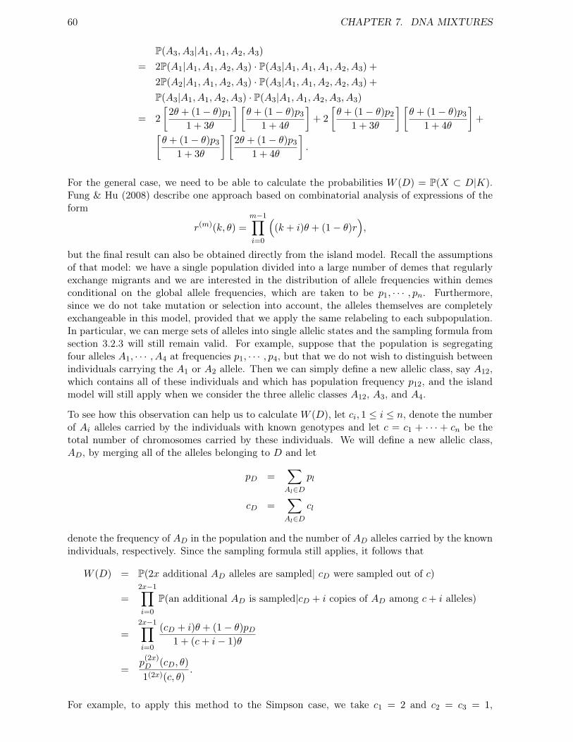
60 CHAPTER 7. DNA MIXTURES
P(A3, A3|A1, A1, A2, A3)= 2P(A1|A1, A1, A2, A3) · P(A3|A1, A1, A1, A2, A3) +
2P(A2|A1, A1, A2, A3) · P(A3|A1, A1, A2, A2, A3) +P(A3|A1, A1, A2, A3) · P(A3|A1, A1, A2, A3, A3)
= 2[
2θ + (1− θ)p1
1 + 3θ
] [θ + (1− θ)p3
1 + 4θ
]+ 2
[θ + (1− θ)p2
1 + 3θ
] [θ + (1− θ)p3
1 + 4θ
]+[
θ + (1− θ)p3
1 + 3θ
] [2θ + (1− θ)p3
1 + 4θ
].
For the general case, we need to be able to calculate the probabilities W (D) = P(X ⊂ D|K).Fung & Hu (2008) describe one approach based on combinatorial analysis of expressions of theform
r(m)(k, θ) =m−1∏i=0
((k + i)θ + (1− θ)r
),
but the final result can also be obtained directly from the island model. Recall the assumptionsof that model: we have a single population divided into a large number of demes that regularlyexchange migrants and we are interested in the distribution of allele frequencies within demesconditional on the global allele frequencies, which are taken to be p1, · · · , pn. Furthermore,since we do not take mutation or selection into account, the alleles themselves are completelyexchangeable in this model, provided that we apply the same relabeling to each subpopulation.In particular, we can merge sets of alleles into single allelic states and the sampling formula fromsection 3.2.3 will still remain valid. For example, suppose that the population is segregatingfour alleles A1, · · · , A4 at frequencies p1, · · · , p4, but that we do not wish to distinguish betweenindividuals carrying the A1 or A2 allele. Then we can simply define a new allelic class, say A12,which contains all of these individuals and which has population frequency p12, and the islandmodel will still apply when we consider the three allelic classes A12, A3, and A4.
To see how this observation can help us to calculate W (D), let ci, 1 ≤ i ≤ n, denote the numberof Ai alleles carried by the individuals with known genotypes and let c = c1 + · · · + cn be thetotal number of chromosomes carried by these individuals. We will define a new allelic class,AD, by merging all of the alleles belonging to D and let
pD =∑Al∈D
pl
cD =∑Al∈D
cl
denote the frequency of AD in the population and the number of AD alleles carried by the knownindividuals, respectively. Since the sampling formula still applies, it follows that
W (D) = P(2x additional AD alleles are sampled| cD were sampled out of c)
=2x−1∏i=0
P(an additional AD is sampled|cD + i copies of AD among c+ i alleles)
=2x−1∏i=0
(cD + i)θ + (1− θ)pD1 + (c+ i− 1)θ
=p(2x)D (cD, θ)1(2x)(c, θ)
.
For example, to apply this method to the Simpson case, we take c1 = 2 and c2 = c3 = 1,

7.2. MULTIPLE CONTRIBUTORS 61
obtaining
P(M |K,Hd) = W (M)−W (M\A3)= W (A1, A2, A3)−W (A1, A2)
=4θ + (1− θ)(p1 + p2 + p3
1 + 3θ· 5θ + (1− θ)(p1 + p2 + p3
1 + 4θ−
3θ + (1− θ)(p1 + p2)1 + 3θ
· 4θ + (1− θ)(p1 + p2)1 + 4θ
,
which can be further simplified with the help of a computer algebra package if desired.

Chapter 8
Statistical Phylogenetics
8.1 Introduction
Our focus in this section will be on the analysis of DNA sequence data and some of its forensicapplications, especially in the growing field of forensic microbiology. Much of the work inthis area has focused on the transmission of infectious diseases, either in a healthcare setting orthrough criminal activity including bioterrorism. One of the key challenges for investigators isto be able to identify the source of a new infection, which can sometimes be done by comparingthe genomes of pathogens isolated from victims with the genomes of pathogens sampled fromthe environment. Some of the more prominent cases have included:
• HIV-1 transmission by a Florida dentist (Ou et al., 1992);
• transmission of HIV-1 during a sexual assault (Sweden: Albert et al., 1994);
• deliberate transmission of HIV-1 (Louisiana: Metzker et al., 2002);
• anthrax attacks: 1993 (Kameido, Japan), 2001 Amerithrax cases (US).
There are a number of important differences between the aims, the methods, and the data usedin human forensic DNA profiling and forensic microbiology. In particular,
• Aims: Genetic profiling seeks to identify the individual contributors of a sample of DNA,whereas forensic microbiology is usually concerned with more distant relationships betweenindividuals and populations.
• Data: Genetic profiling still largely relies on STR markers, whereas forensic microbiologyoften (but not always) uses DNA sequence data.
• Data: Mutation can often be neglected in genetic profiling, but must be accounted for inforensic microbiology.
• Analysis: Mendelian analysis is the main tool used to interpret human genetic profiles,while statistical phylogenetics and population genetics are more important in forensic mi-crobiology.
Phylogenetic analysis is concerned with establishing the evolutionary relationships that holdwithin a group of individuals. This can be done by exploiting the fact that related individualstend to share similar characters which they have inherited from common ancestors. These char-acters can include both morphological and behavioral traits, but most phylogenetic analyses of
62
8.1. INTRODUCTION 63
extant species (and even of some extinct species) now rely almost exclusively on genetic sequencedata. The relationships between the individuals in a sample can be represented as a phyloge-netic tree (also called a genealogy), which is a connected graph without cycles. The nodesin a phylogenetic tree correspond either to the sampled individuals (the leaves of the tree) orto common ancestors of groups of these individuals, while the branches in a tree correspond tolineages. A tree can either be rooted, in which case there is a single internal node that is thecommon ancestor of all of the individuals in the sample (the most recent common ancestor),or the tree can be unrooted if such a node is not designated. Rooted trees have a naturalorientation, in which branches are regarded as directed edges that point away from the root andtowards the leaves. A phylogenetic tree can encode two kinds of information: the topology ofthe tree shows groups of individuals that are more closely related to one another than to anyother individual in the sample, while the branch lengths may indicate the absolute or relativetime that has elapsed since a group of individuals last shared a common ancestor. A tree is saidto be binary if every node has either one or three neighbors (two nodes are said to be neighborsif they are connected by a single branch): leaves have exactly one neighbor, while all other nodeshave three. Phylogenetic trees are often, but not always, binary: for example, it is not alwayspossible to resolve the order in which a rapid series of branching events has occurred, in whichcase these may be collapsed into a polytomy. One of the main challenges faced in phylogeneticsis that even if we restrict attention to binary trees, the number of such trees grows more thanexponentially rapidly as a function of the number of individuals in the sample. In particular, thenumber of unrooted binary trees with n labeled leaves is
(2n− 5)!! =(2n− 4)!
(n− 2)!2n−2= 1× 3× 5× · · · × (2n− 5)
while the number of rooted binary trees is (2n − 3)!!, which is even larger. For example, whenn = 20, these numbers are approximately 2.22×10²⁰ and 8.2×10²¹, respectively, i.e., they are toolarge to allow exhaustive enumeration of all possible binary trees in the course of a phylogeneticanalysis.
In part because of the combinatorial difficulty of the problem, many methods have been proposedfor phylogenetic analyses. These include:
• distance methods (e.g., neighbor-joining): these methods only consider the matrixof pairwise distances between taxa;
• parsimony methods: these methods try to find the tree that requires the least numberof weighted changes in character states;
• likelihood inference: these methods try to find the tree that has the highest likelihoodunder a model of character evolution;
• Bayesian phylogenetics: these methods try to generate a sample of trees from theposterior distribution.
Because parsimony and likelihood methods require the optimization of an objective functionover the space of all possible trees, it is usually not possible to implement these methods exactlywhen working with more than about 6 taxa. Instead, heuristic methods are used to examinea subsample of all possible trees that ideally will include, if not the optimal tree itself, thenat least some tree that is ‘close’ in some sense to the optimal tree. A similar problem arises inBayesian phylogenetics, where the posterior sample of trees may not be large enough to accuratelyapproximate the true posterior distribution.

64 CHAPTER 8. STATISTICAL PHYLOGENETICS
8.2 Substitution Processes
To do statistical phylogenetics, we need to be able to calculate the conditional probability of theobserved data (in terms of character traits or genetic sequences) as a function of the evolution-ary relationships between the sampled individuals. Usually this is done by adopting a stochasticmodel that describes how the characters in question evolve as they are transmitted along eachbranch of the tree. It is also usually assumed that evolutionary changes occur independentlyalong different branches of the tree. While this assumption may not apply to characters sub-ject to common selection pressures operating on different lineages, it is probably a reasonableapproximation when modeling neutral evolution.
In molecular phylogenetics, the models used to describe the evolution of DNA and RNA sequencesas they are transmitted from one generation to the next are called substitution processes.Although substitution and mutation are closely related, there is an important difference, whichis that a mutation in a DNA sequence only leads to a substitution if it is transmitted from onegeneration to the next. Furthermore, although the two processes coincide at neutrally evolvingsites, the rate of substitution at a non-neutral site may be less than or greater than the mutationrate at that site depending on whether natural selection impedes or favors the transmission ofnew mutations to the next generation. For example, there is a large body of evidence that thesubstitution rate in coding DNA is strictly less than the mutation rate and that this is becausesome mutations are deleterious and so are removed from populations by natural selection.
To describe the substitution processes that are commonly used in molecular phylogenetics, Ifirst need to introduce some background material on stochastic processes and continuous-timeMarkov chains. Suppose that E = e1, e2, · · · , en is a finite set. An E-valued continuous-timestochastic process is simply a sequence of random variables Xt, t ≥ 0 with the property thateach variable Xt is a random variable with a value in E. The process is said to be continuous intime because the random variables Xt are indexed by a parameter that can be any non-negativereal value. Here we interpret Xt as the state of a system of interest at time t.
A continuous-time stochastic process (Xt; t ≥ 0) is said to be a continuous-time Markovchain (CTMC) if it has the property that for any set of times s < t < u, the random variablesXs and Xu are conditionally independent given the value of Xt. This is called the Markovproperty and it means that if we know the current value of the process, say Xt = x, then wecan predict the future values of the process without having to know how the process came toarrive at state x at time t. Since there are potentially infinitely many ways in which the processcould have arrived at this particular state, Markov processes are much easier to work with thanare stochastic processes that lack the Markov property. In particular, one can use the Markovproperty to show that any CTMC X = (Xt; t ≥ 0) with values in the set E can be described bya matrix Q, called the rate matrix of X, and by the initial distribution µ of the variable X0.If E contains n different states, then the rate matrix Q = (qij) is an n × n-dimensional matrixwith entries qij ≥ 0 that specify the transition rate from state ei to state ej when j 6= i. Also,by convention, the diagonal elements qii of the rate matrix are chosen so that the sum of theelements in each row is equal to 0: for each i = 1, · · · , n, we set
qii = −∑j 6=i
qij .
Notice that the absolute value of the diagonal element |qii| is just the total rate at which theprocess transitions from state i to some other state.
Given the rate matrix Q and the initial distribution µ, the behavior of the chain X has thefollowing simple description. We first choose a point from E at random according to the initialdistribution µ and we set X0 equal to this value. If this state is ei, say, we then simulate an

8.2. SUBSTITUTION PROCESSES 65
exponentially-distributed random variable τ0 with mean 1/|qii|, which determines how long theprocess remains within its initial state. τ0 is said to be the holding time in the initial state.Recall that the density of an exponential random variable with this mean is
pτ0(t) = |qii|e−|qii|t, t ≥ 0
and notice that the duration of this holding time will usually be inversely proportional to thetotal transition rate out of state ei. At time τ0, the chain jumps to a new state in E that ischosen according to the following probability distribution: given that the initial state is ei, thenew state is chosen to be ej with probability
qij/|qii|.
In other words, the larger the transition rate from state ei to ej is, the more likely it is that thechain will move to ej rather than to some other state. In particular, if qij = 0 for some j, thenthe probability that the chain moves to state ej is 0. Furthermore, if we know the initial state ofthe chain, then the holding time in that state and the new state to which the chain jumps at theend of the holding time are independent of one another. This is a consequence of the Markovproperty.
The future behavior of the chain is determined similarly. Following the k’th jump, the chain willoccupy a new state, say el, and the holding time in that state will be an exponentially-distributedrandom variable τk with mean 1/|qll|. At the end of the holding time, the chain will jump to anew state em in E that is chosen according to the probability distribution with weights
qlm/|qll|.
This state depends only on the state occupied by the chain immediately before the jump, butit is independent of both the holding times τ0, · · · , τk and of the states occupied by the chainprior to the k’th jump. These assertions too are consequences of the Markov property. Theconstruction described in this paragraph can be used to simulate Markov chains on a computerand is known as the Gillespie algorithm.
One of the most fundamental questions that we can ask about a Markov chain concerns theprobability that the chain is in state ej at time t given that it was in state ei at time 0. Thisquantity is called the transition probability from state ei to ej at time t and the n×n matrix
P (t) = (pij(t))
is called the transition matrix. The transition probabilities can be found by solving thefollowing system of first-order linear differential equations,
P (t) = P (t)Q,
which are known variously as the master equations or the forward Kolmogorov equations.For fixed i, j, the corresponding equation has the form
pij(t) =∑k 6=j
qkj · pik(t)− |qjj | · pij(t).
An explicit solution can be found by exponentiating the rate matrix and is equal to
P (t) = eQt ≡∞∑n=0
1n!Qntn,
where Qn = Q · · ·Q is the usual matrix product.

66 CHAPTER 8. STATISTICAL PHYLOGENETICS
Example 8.1. Suppose that X = (Xt; t ≥ 0) is a CTMC with state space is E = 1, 2 and thatthe rate matrix is
Q =(−a ab −b.
),
i.e., a is the transition rate from 1 to 2, while b is the transition rate from 2 to 1. Since thereare only two states, we know that the transition probabilities out of each state must sum to 1:
p11(t) + p12(t) = 1p21(t) + p22(t) = 1.
These can be used to simplify the Kolmogorov forward equations
p11(t) = −ap11(t) + bp12(t)= b− (a+ b)p11(t)
p22(t) = −bp22(t) + ap21(t)= a− (a+ b)p22(t),
which can then be solved to give
P (t) = eQt =1
a+ b
(b+ ae−(a+b)t a− ae−(a+b)t
b− be−(a+b)t a+ be−(a+b)t.
)In particular, if a+ b > 0, then as t tends to infinity, this matrix tends to the limit
P (∞) =1
a+ b
(b ab a
),
which shows that after a large amount of time has elapsed, the chain ‘forgets’ its initial state andis found in state 1 with probability b/(a+ b) and state 2 with probability a/(a+ b).
The limiting probability distribution found in the preceding example is said to be a stationarydistribution or equilibrium distribution for the Markov chain. In general, a probabilitydistribution π on the state space E is said to be a stationary distribution for a Markov chainX with values in E if whenever the initial distribution is π, then the distribution of the chainat every time t ≥ 0 is π. Every Markov chain with values in a finite state space E has at leastone stationary distribution and some chains have more than one stationary distribution. (Takea = b = 0 in the previous example for an example of a chain with infinitely many stationarydistributions.) Some Markov chains have a much stronger property, called ergodicity, whichmeans that their distributions at large times t converge to a unique stationary distribution πas t → ∞ no matter what the initial distribution is. This is true of the chain in the previousexample whenever a, b > 0.
Substitution processes in molecular evolution are usually modeled using continuous-time Markovchains either on the set of four nucleotides E = T,C,A,G or E = U,C,A,G for DNA orRNA sequences, respectively, or on the set of 64 possible triplet codons. Codon-based modelsare important when modeling the evolution of coding sequences, but here we will concentrateon nucleotide-based models for DNA sequence evolution. We will also adopt an arbitrary orderfor the four bases, setting e1 = T, e2 = C, e3 = A, e4 = G and noting that different authors usedifferent conventions. Implicit in writing down such a model is the common assumption thatsubstitution processes at different sites are independent of one another.

8.2. SUBSTITUTION PROCESSES 67
Example 8.2. The Jukes-Cantor model is the simplest CTMC process used to model the neutralsubstitution process at a single site in a DNA molecule. It assumes that substitution rate fromany one base to any other is a constant µ, so that the rate matrix is just
Q =
−3µ µ µ µµ −3µ µ µµ µ −3µ µµ µ µ −3µ
,
while the transition matrices are given by
P (t) = eQt =14
1 + 3e−4µt 1− e−4µt 1− e−4µt 1− e−4µt
1− e−4µt 1 + 3e−4µt 1− e−4µt 1− e−4µt
1− e−4µt 1− e−4µt 1 + 3e−4µt 1− e−4µt
1− e−4µt 1− e−4µt 1− e−4µt 1 + 3e−4µt
.
In particular, if we let t → ∞, then we see that the Jukes-Cantor model is an ergodic Markovchain with stationary distribution (1/4, 1/4, 1/4, 1/4), i.e., this model implies that all four basesoccur at equal frequencies at equilibrium.
If we compare homologous sites in the genomes of two individuals that shared a common ancestort units of time ago, then under the Jukes-Cantor model, the probability that the two sites areidentical is (1 + 3e−8µt)/4, while the probability that they differ is 3(1− e−8µt)/4. Now, supposethat we compare L homologous sites between these two individuals and assume that each siteevolves at the same rate according to the Jukes-Cantor model and that the substitution processesat the different sites are independent. If we know the mutation rate µ (expressed in mutationsper site per unit time), then this model can be used to estimate the divergence time between thetwo individuals. In particular, if there are d sites at which the two genotypes differ, then thelikelihood function for t (treated as a parameter) is
L(t; d) =
(3(1− e−8µt
)4
)d(1 + 3e−8µt
4
)L−d,
while the log-likelihood function is
l(t; d) = C + d log(1− e−8µt
)+ (L− d) log
(1 + 3e−8µt
),
where C is a constant that does not depend on t. The maximum likelihood estimate of t can befound by differentiating the log-likelihood function with respect to t and setting this equal to 0.This gives the equation
0 = d8e−8µt
1− e−8µt+ (L− d)
−24e−8µt
1 + 3e−8µt,
which can be solved explicitly. (To do so, first let x = e−8µt and solve for x, and then solve fort.) After some algebra, we find that the maximum likelihood estimate of the divergence time isequal to
t =−18µ
log(
1− 43d
L
),
provided that d/L < 3/4. When d/L 1, then the estimated divergence time is approximatelylinear in the proportion of sites that differ,
t ≈ 16µ
d
L,
but this approximation breaks down as d/L increases due to the occurrence of multiple mutationsat sites. In particular, some fraction of substitutions will go unobserved due to reverse mutations

68 CHAPTER 8. STATISTICAL PHYLOGENETICS
that restore the ancestral nucleotide, e.g., T may mutate to A which can then mutate back toT . This phenomenon is known as saturation and makes it difficult to accurately estimate largedivergence times (although lower bounds can be given).
Although the Jukes-Cantor model is important for historical reasons, the assumption that allfour bases mutate at equal rates to all other bases is known to be too simplistic a model for theevolution of most DNA sequences. For this reason, more general models have been introducedand the one that has perhaps seen the widest application in molecular phylogenetics is called thegeneral time reversible (GTR) model, which has the following rate matrix
Q =
πCα πAβ πGγ
πTα πAδ πGεπTβ πCδ πGηπTγ πCε πAη
,
where (πT , πC , πA, πG) is the stationary distribution for this model, α, β, γ, δ, ε, η are six freeparameters (to be estimated from data), and the circles on the diagonal indicate that theseentries should be chosen so that the row sums are zero. Although an analytical expression forthe transition matrix P (t) = eQt can be written down for the GTR process, it is very complicatedand these probabilities are often calculated by numerical evaluation of the matrix exponential.The process is said to be time reversible because it satisfies the following condition,
π(ei) · P(Xt+s = ej |Xt = ei) = ·π(ej)P(Xt+s = ei|Xt = ej),
which says that, at equilibrium, the transition probabilities of the Markov chain do not changeif we reverse the direction of time. While this condition has no biological justification, it isa convenient assumption because it allows us to calculate the likelihoods of unrooted trees byassigning an arbitrary direction to the flow of time. In fact, the GTR model is the most generalclass of CTMC on the state space E = T,C,A,G with this property and several other substi-tution processes commonly encountered in molecular phylogenetics, including the Jukes-Cantormodel, are themselves special cases of the GTR. One model of particular importance is called theHKY85 model (after the three authors who proposed it in 1985, Hasegawa, Kishino and Yano).It accounts for the different rates at which transitions and transversions occur and has a ratematrix that can be expressed as
Q =
πCκ πA πGπTκ πA πGπT πC πGκπT πC πAκ
,
where the parameter κ is interpreted as the transition/transversion rate ratio. In humans, typicalvalues of κ are around 2 with some variation between coding and non-coding loci.
8.3 Branching Processes and Coalescents
In Bayesian phylogenetics, inference is based on the posterior distribution of phylogenetic treesgiven by the formula:
p(T ,Θ|D) = p(D|T ,Θ)p(T ,Θ)p(D)
(8.1)
where D is the sequence data, T is a phylogenetic tree, and Θ is a set of model parameterssuch as the substitution rate matrix. The conditional probability p(T ,Θ|D) is said to be the

8.3. BRANCHING PROCESSES AND COALESCENTS 69
posterior distribution of T and Θ and it depends on both the likelihood of the data givenby p(X|T ,Θ) and also on the prior distribution p(T ,Θ) of the tree and model parameters.The unconditional probability p(D) can be regarded as a normalizing constant and usually doesnot play a role in inference.
It is often the case that the set of model parameters can be decomposed into two disjoint sets,
Θ = ΘT ∪ΘS ,
where ΘT contains parameters that govern the prior distribution of the phylogenetic tree andΘS contains any parameters that are independent of the tree. We can then write the joint priordistribution on T and Θ as the product
p(T |ΘT )p(ΘT ,ΘS), (8.2)
while the likelihood function can often be expressed as
p(D|T ,ΘS), (8.3)
i.e., once we condition on the tree, the data only depends on the parameters in ΘS . If thephylogenetic tree is the only object of interest, then one can obtain the posterior distribution ofT alone by integrating over Θ in equation (8.1):
p(T |D) =1
p(D)
∫p(D|T ,ΘS)p(T |ΘT )p(ΘT ,ΘS)dΘTdΘS . (8.4)
It is almost always the case that this integral cannot be evaluated analytically or even numericallyand then Monte Carlo methods are used to estimate its value.
Our purpose in this section is to describe some of the prior distributions on phylogenetic trees thathave found to be useful in Bayesian phylogenetics. Recall that the role of the prior distribution inBayesian statistics is to summarize any existing knowledge or beliefs that we may have about theunknown elements of a statistical model before we examine the new data that is to be explained bythe model. In Bayesian phylogenetics, this prior information could take into account alternativedata sources such as fossil evidence, but often it comes from mathematical theories that describethe distribution of trees that are expected under a particular model of evolution or demography.Here we consider two classes of models known as branching processes and coalescent processes.
8.3.1 Branching Processes
A continuous-time branching process is a continuous-time Markov chain X = (Xt; t ≥ 0) thatdescribes the growth of a population in which each individual reproduces independently of therest of the population. The variable Xt specifies the number of individuals alive at time tand the population is said to be extinct at time t if Xt = 0. The behavior of a branchingprocess depends on two parameters: the branching rate λ > 0 and the offspring distribution νwhich is a probability distribution on the non-negative integers. Gillespie’s algorithm can beused to simulate a branching process in the following manner. If Xt = n, choose one of the nindividuals at random and generate both an exponentially distributed random variable τ withmean 1/(λn) and an integer-valued random variable ξ with distribution ν. τ and ξ are assumedto be independent of each other and of the past history of the population. Then, at time t+ τ ,replace the chosen individual by its ξ descendants and set Xt+τ = n− 1 + ξ. Although X itselfis an integer-valued process that only records the population size at different times, notice thatour description of this process also tells us how to construct the random tree that describes thegenealogical relationships between the individuals in the population.

70 CHAPTER 8. STATISTICAL PHYLOGENETICS
The Yule process (also called the Yule-Ferry or the pure birth process) is an important specialcase of the general continuous-time branching process in which every reproduction event resultsin the birth of exactly two new individuals. In this case the tree is binary and the populationincreases by one at each branching event. In fact, one can use the forward equations to solvefor the probability distribution of the number of individuals alive at time t. For example, if thepopulation is initially founded by a single individual, then X0 = 1 and it can be shown that Xt
is a geometrically-distributed random variable with mean eλt, i.e.
P(Xt = n) = e−λt(
1− e−λt)n−1
, n ≥ 1.
In Bayesian phylogenetics, the Yule process as well as other more complicated branching processesare sometimes used to specify the prior distribution on the phylogenetic tree that describes theevolutionary relationships amongst a group of species. In other words, the prior probability of aparticular tree T is set equal to the probability density of that tree under the chosen model. Whenthe Yule process is used, there is one tree-related parameter λ which determines the branchingrate. The value of λ can either be estimated from the data or be given a prior distribution itselfas in equation (8.2).
8.3.2 Coalescent Processes
The phylogenetic tree of a sample of individuals from a single randomly-mating populationof constant size has a well-studied description in terms of a class of continuous-time Markovchains known as coalescent processes. Recall that in the Wright-Fisher model (cf. Section3.2), the parents of the N individuals alive in generation t + 1 are determined by samplingN times at random and with replacement from amongst the individuals alive in generation t.Although we were previously interested in this model for what it could tell us about the effect ofrandom genetic drift on the amount of genetic variation maintained in a finite population, theconstruction described in the previous sentence can also be used to determine the genealogy ofa random sample of individuals taken from a given generation. For example, if we sample justtwo individuals from generation t, then the probability that they share a common ancestor ingeneration t−1 is 1/N . If they don’t share a common ancestor in the preceding generation, thenthe probability that they share a common ancestor two generations ago is (1− 1/N) · 1/N , whilethe probability that they first share a common ancestor k generations ago is(
1− 1N
)k−1
· 1N.
In other words, if we write τ2 for the number of generations in the past when the two individualsfirst shared a common ancestor, then τ2 is a geometrically-distributed random variable with meanN . The two lineages of ancestors to these individuals are said to coalesce (i.e., come together)at time τ2 and τ2 is called the coalescent time for the two lineages.
If three individuals are sampled at random from the same population, then the probability thatall three share a common ancestor in the preceding generation is N−2. When N is large, thisprobability is much smaller than the probability that exactly two of the individuals share acommon ancestor in that generation, which can be written as
3N
+O
(1N2
).
The factor of three in the first term accounts for the fact that there are three distinct pairs ofindividuals that could share a common ancestor in the preceding generation. Similar statementsapply to earlier generations and it can be shown that when N is large, the genealogy of a random

8.3. BRANCHING PROCESSES AND COALESCENTS 71
sample of three individuals is much more likely to be a binary tree than to contain a complexcoalescent event involving the simultaneous merger of more than two ancestral lineages. In fact,this remains true even when we consider samples containing a larger number of individuals, sayn, provided that n is much smaller than N .
A simple approximation for the genealogy of a random sample of n individuals can be derivedby measuring time in units of N generations and taking the limit as N tends to infinity with nfixed. It can be shown that only pairwise coalescent events occur and that the time to the nextcoalescent event when there are k lineages in the tree is exponentially distributed with meanequal to (
k
2
)−1
=2
k(k − 1).
In fact, the genealogy of a random sample of n individuals can be generated in the followingmanner. We first generate an exponentially-distributed random variable τn with mean
(n2
)−1.At that time, two of the lineages in the tree are chosen uniformly at random and merged into asingle lineage. We next generate an independent exponentially-distributed random variable τn−1
with mean(n−1
2
)−1 and then choose two of the remaining n − 1 lineages in the tree at randomand merge them into a single lineage. This process continues until only a single lineage is leftand the time, say TMRCA, when this first occurs is said to be the time to the most recentcommon ancestor (TMRCA) of the sample. A formal description of this process was first givenby J.F.C. Kingman in 1983 and consequently the process has come to be known as Kingman’scoalescent. Notice that the expected value of the TMRCA is equal to
E [TMRCA] = E [τn + τn−1 + · · ·+ τ2]
=n∑k=2
2k(k − 1)
= 2n∑k=2
(1
k − 1− 1k
)= 2
(1− 1
n
),
where we recall that time is measured in units of N generations. Because the rate of coalescenceis a quadratic function of the number of lineages in the tree, branches near the top of a coalescenttree tend to be much shorter than branches close to the root.
Although we obtained Kingman’s coalescent by way of the Wright-Fisher model, Kingman andothers have shown that this particular process provides a surprisingly accurate approximationfor the distribution of genealogies obtained from a much larger class of models of genetic driftprovided that the following conditions are satisfied:
• the population size N is large and constant;
• the sample size n is much smaller than N ;
• the population is randomly mating;
• the variance in reproductive success is not too large;
• the individuals are selectively equivalent (neutral evolution).
Various generalizations of the coalescent have been derived which allow some of these conditionsto be relaxed. Provided that the population never becomes too small (i.e., no bottlenecks),variable population sizes can be accommodated by a simple change in the rate of coalescence.

72 CHAPTER 8. STATISTICAL PHYLOGENETICS
In fact, by stipulating a parametric model of population size change such as exponential growth,e.g.,
Nt = N0eγt,
one can use Bayesian phylogenetic methods to infer the demographic history of a population froma sample of DNA or RNA sequences. Spatial structure is arguably the most important featureof real populations that has not yet been adequately addressed by coalescent-based phylogeneticanalyses, but some progress in this direction has been made in recent years (cf. Lemey et al.2009, PLoS Comput. Biol.).


![Lectures at the International Summer School on Fundamental ... · arXiv:cond-mat/0109419v2 [cond-mat.str-el] 23 Nov 2001 Quantumphasetransitionsofcorrelated electronsintwodimensions](https://static.fdocuments.us/doc/165x107/5ffe20a0f462ba2aac5bf76f/lectures-at-the-international-summer-school-on-fundamental-arxivcond-mat0109419v2.jpg)


![[XLS] for the month Apr... · Web viewMargin MarketType MarketType MarketType MarketType MarketType_Text MarketType_Text Mast Mast Mat Mat Mat Mat Mat Mat Mat Mat Mat Mat Mat Match1](https://static.fdocuments.us/doc/165x107/5ab4774c7f8b9a2f438b92c4/xls-for-the-month-aprweb-viewmargin-markettype-markettype-markettype-markettype.jpg)