Lecture4 - University of Edinburgh · The law of diminishing marginal returns is huge in economics....
62
Firms and Production Lecture 4 Reading: Perlo/ Chapter 6 August 2015 1 / 62
Transcript of Lecture4 - University of Edinburgh · The law of diminishing marginal returns is huge in economics....

Firms and Production
Lecture 4
Reading: Perlo¤ Chapter 6
August 2015
1 / 62

Introduction
In this lecture we look at �rms and production.
It is the �rst step in deriving the supply curve we say in the �rstlecture.
2 / 62

Outline
Ownership and Management of Firms - What exactly is a "�rm?"Production - How a �rm makes output from their set of inputs.
Short-Run Production - Look at production when the �rm has a�xed input.
Long-Run Production - Look at production when there are no �xedinputs.
Returns to Scale - How the size of a �rm a¤ects how much itproduces.
Productivity and Technical Change - The most output you can getfor your inputs varies across �rms and across time.
3 / 62

Ownership and Management of Firms
A �rm is simply some organization that takes inputs and turns it intooutputs.
We can roughly divide these �rms into
private sectorpublicnon-pro�t �rms
4 / 62

Ownership and Management of Firms
Sole proprietorship
owned by an individual who is responsible for all debts.Example: A freelance writer or a bookkeeper.
5 / 62

Ownership and Management of Firms
General partnership
Jointly owned by multiple people who are together responsible fordebts.Example: Law o¢ ce with multiple partners.
6 / 62

Ownership and Management of Firms
Corporations
Owned by shareholders in proportion to the amount of stock they own.limited liability.Example: Microsoft, recently Facebook.
7 / 62

Ownership and Management of Firms
Private �rms have the single goal of maximizing pro�ts.
Pro�t (π) is de�ned as total revenue (TR) minus total cost (TC ).
π = TR � TCTR = p � q
A �rm can only maximize pro�t if it achieves technical e¢ ciency.Technical e¢ ciency means they get the most output they possibly canfrom their set of inputs and technology.
8 / 62
Production
A �rm takes inputs (factors of production) and turns it into outputaccording to its technology.
We can broadly classify these inputs into capital (K), labour (L) andmaterials (M) (which we usually ignore for simplicity).
9 / 62

Production
The production function summarizes this process, and tells usexactly how much output the �rm can get from their inputs.
For example suppose our production function is
q = f (L,K ) = 2 � L �K
If the �rm employs two units labour and 4 units of capital it gets 16units of output (it could produce less, but that would not be e¢ cient).
10 / 62

Production
EXAMPLE
Suppose a �rm produces output using only labour according to theproduction function q = L2.
Sketch this production function and identify two production plans,one that is technically e¢ cient and one that is not.
11 / 62
Production
The short run is the period of time that at least one factor ofproduction cannot be changed.
For example, dominoes can decide how many delivery drivers it hiresin a month, but can�t decide how many stores to build in this timeframe.
12 / 62
Production
The long run is a period of time in which all inputs can be varied.The di¤erence between short and long run varies by industry.
We call inputs that can�t be changed �xed inputs, and ones that canbe changed variable inputs.
13 / 62

Short-Run Production
Lets say capital is �xed in the short run, our production function isthen
q = f (K , L)
Suppose our production function is q = 2KL, but capital is �xed atK = 4 in the short-run.
Our short-run production function becomes q = 8L.
We can summarize the relationship between output and the amountof labour used by the total product of labour, the averageproduct of labour and the marginal product of labour.
14 / 62

Short-Run Production
Total product of labour is the amount of output that a givenamount of labour can produce holding other inputs �xed
Marginal product of labour is the extra output you get fromincreasing labour by some in�nitesimally small amount
MPL =∂q∂L
Average product of labour is the amount of output produced perworker
APL =qL
15 / 62

Short-Run Production
EXAMPLE
Suppose our production function is
Q = K � L2
What is the total product of labour, marginal product of labour andaverage product of labour if capital is �xed at 50?
16 / 62

Short-Run Production
If our short run production function is q = L+ 30L2 � L3
17 / 62

Short-Run Production
We assume the �rm can hire fractions of workers (which is why this issmooth)
The MPL is the slope of the production function
The APL is the slope of the chord from the origin
18 / 62

Short-Run Production
The previous production function is typical
APL initially rises because of gains from specialization, but it declinesbecause capital is held constant.
19 / 62

Short-Run Production
The MPL always intersects the APL at the maximum of the APLcurve.
When MPL > APL, the average is pulled up.
When MPL < APL, the average is pulled down.
20 / 62

Short-Run Production
EXAMPLE
Let�s prove together that MPL = APL at the maximum of APL forthe production function q = L+ 30L2 � L3.
21 / 62

Short-Run Production
The law of diminishing marginal returns is huge in economics.As you increase one input, holding all other inputs and technologyconstant, the marginal returns to that input will decrease eventually.
The second derivative will become negative.
You can�t grow the world�s food supply in a �ower pot.
This is why Malthus predicted mass starvation (one input -land- is�xed).
22 / 62

Short-Run Production
For the production function
q = L+ 30L2 � L3
MPL =dqdL= 1+ 60L� 3L2
23 / 62
Short-Run Production
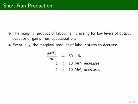
The marginal product of labour is increasing for low levels of outputbecause of gains from specialization.
Eventually, the marginal product of labour starts to decrease.
dMPLdL
= 60� 6LL < 10 MPL increases
L > 10 MPL decreases
24 / 62

Short-Run Production
EXAMPLE
Suppose the world�s supply of food is determined by the productionfunction
F = M12 L
12
M is land and is �xed at 3600.
L is labour.
At what point does this production function exhibit diminishingmarginal returns to labour?
25 / 62

Long-Run Production
In the long run, the �rm is free to select as much of any input...nothing is �xed.
Lets suppose our production function is Cobb-Douglas
q = 3L12K
12
Try to graph this.
26 / 62
Long-Run Production
Now that we have multiple variable inputs, our production functionhas multiple dimensions.
Can�t really deal with it graphically.
We can summarize this production function in 2 dimensions.
27 / 62

Long-Run Production
An isoquant is a curve that shows the e¢ cient combinations ofinputs that produce a single level of output
This has a very similar interpretation to indi¤erence curves.
Every combination of labour and capital on the same isoquant willproduce the same amount of output.
28 / 62

Long-Run Production
29 / 62

Long-Run Production
Say our production function is
Q = 10 �K � L
Draw the isoquant for Q = 10 and Q = 20.
30 / 62

Long-Run Production
Lets now discuss the properties of isoquants.
1. Further from the origin, the greater the output
The more inputs you use, the more output you get if you areproducing e¢ ciently
31 / 62

Long-Run Production
2. They cannot cross
Suppose the isoquant where Q = 20 and Q = 15 cross.
The �rm could produce 15 or 20 units of output for the same inputcombination.
The �rm would not be e¢ cient if it produced 15 for that inputcombination.
32 / 62

Long-Run Production
3. They slope downward
If they sloped upward, the �rm could produce the same level ofoutput with fewer inputs.
33 / 62

Long-Run Production
4. They are thin
If they were thick, the �rm could decrease its input use and get thesame level of output
34 / 62

Long-Run Production
5. UNLIKE indi¤erence curves, isoquants are a cardinal measure.
Output is objective, it is not some abstract thing like utility.
35 / 62

Long-Run Production
The curvature of the isoquant tells us howsubstitutable/complementary the inputs are in the production process.
The more "curvy" the isoquant, the greater degree ofcomplementarity there is between inputs
36 / 62
Long-Run Production
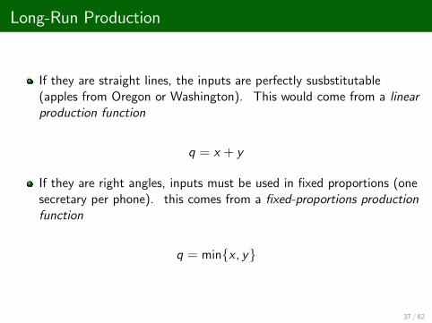
If they are straight lines, the inputs are perfectly susbstitutable(apples from Oregon or Washington). This would come from a linearproduction function
q = x + y
If they are right angles, inputs must be used in �xed proportions (onesecretary per phone). this comes from a �xed-proportions productionfunction
q = minfx , yg
37 / 62

Long-Run Production
38 / 62

Long-Run Production
The slope of the isoquant shows the �rm�s ability to replace one inputwith another holding output constant.
This is called the marginal rate of technical substitution (MRTS) .How much K can we give up for another unit of L holding outputconstant.
39 / 62
Long-Run Production
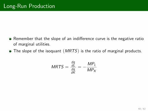
Remember that the slope of an indi¤erence curve is the negative ratioof marginal utilities.
The slope of the isoquant (MRTS) is the ratio of marginal products.
MRTS =dqdLdqdK
= �MPLMPK
40 / 62

Long-Run Production
EXAMPLE
Lets �nd the MRTS of
q = ALαK 1�α
Is the MRTS constant for this production function?
41 / 62

Long-Run Production
If we have normal convex isoquants, we have a diminishing marginalrate of substitution
That is, when a lot of capital and little labour is used, the MRTS isreally high. When a lot of labour and a little capital is used, it isreally low.
42 / 62

Long-Run Production
Suppose we have a factory with 1,000,000 workers and only onemachine.
To keep output constant, we could trade one machine for a ton ofworkers (because workers need machines)
As we get more machines, the number of workers we can trade forone more machine will decrease.
43 / 62

Long-Run Production
44 / 62

Long-Run Production
For most isoquants, the MRTS is not constant.
As we increase capital and decrease labour, at what rate does theMRTS change?
This is the elasticity of substitution... A measure of how "curvy"our isoquants are
45 / 62

Long-Run Production
Elasticity of substitution (σ) is the percentage change in the capitallabour ratio w.r.t a percentage change in the MRTS
σ =
d (K/L)K/L
dMRTSMRTS
=d(K/L)dMRTS
MRTSK/L
If σ is really high, that means a tiny change in the MRTS results in abig change in K/L, the isoquant is pretty �at.
46 / 62

Long-Run Production
EXAMPLE
What is the elasticity of substitution for the following Cobb-Douglasproduction function?
Q = ALαK β
What is the elasticity of substitution for a linear production function?
What does that mean?
47 / 62

Returns to Scale
If we increase our inputs proportionately, what happens to our output?
This is called returns to scaleWe can have increasing, decreasing or constant returns to scale.
48 / 62

Returns to Scale
If doubling our inputs leads to exactly double the output, we haveconstant returns to scale
2f (L,K ) = f (2L, 2K )
49 / 62

Returns to Scale
If doubling our inputs leads to more than double the output, we haveincreasing returns to scale
2f (L,K ) < f (2L, 2K )
Could be caused by greater specialization
50 / 62

Returns to Scale
If doubling our inputs leads to less than double the output, we havedecreasing returns to scale
2f (L,K ) > f (2L, 2K )
Could be caused by management or organizational problems
51 / 62

Returns to Scale
What industries do you think have constant, increasing or decreasingreturns to scale?
What are some factors that determine returns to scale?
52 / 62

Returns to Scale
Generally speaking, our production function is homogenous of degreeγ when
f (xL, xK ) = xγf (L, k)
53 / 62

Returns to Scale
EXAMPLE
The following production function is homogenous of degree what?
Q = K12 L
14
54 / 62

Returns to Scale
It is possible for production functions to have varying returns to scale.
Could have increasing returns to scale for low levels of production,and decreasing returns to scale for high levels of production.
For low levels of production, you have gains to specialization and forlarge levels of production, you run into management problems.
55 / 62

Returns to Scale
56 / 62
Productivity and Technical Change
Even if two �rms are producing e¢ ciency, it is possible that they arenot equally as productive.
We can express a �rm�s relative productivity by the ratio of the �rm�soutput q to the amount of output the most productive �rm in theindustry could have produced from the same inputs q�
ρ =qq�� 100
If you are the most productive �rm in the industry, what is ρ?Estimated that the average productivity of manufacturing �rms in theUS is 63% to 99%.
57 / 62

Productivity and Technical Change
It is possible that one �rm can produce more today from a givenamount of inputs than it could in the past.
An advance in knowledge that allows more output to be producedfrom the same level of inputs is called technical progress.Can be neutral or non-neutral.
58 / 62

Productivity and Technical Change
Neutral technical change means the �rm can produce more outputusing the same ratio of inputs.
q = A(t)f (L,K )
For example
q1 = 10 �K .5L.5
q2 = 100 �K .5L.5
59 / 62

Productivity and Technical Change
Or it can be non-neutral in which innovations alter the proportion ofinput used.
q1 = 10 �K .5L.5
q2 = 10 �K .5L.8
If a machine is invented that requires only one person to operate itrather than two, this is a non-neutral labour saving technical change.
60 / 62

Summary
What is technical e¢ ciency?
What does a production function show you?
What is the di¤erence between the short and long run?
61 / 62

Summary
What causes diminishing marginal returns?
What is an isoquant
What is the marginal rate of substitution and the elasticity ofsubstitution?
What are returns to scale?
What is the di¤erence between a neutral and non-neutral technicalchange?
62 / 62