Lecture 3Bone Mechanics and Remodelling

http://www.aeromech.usyd.edu.au/people/academic/qingli/MECH4961.htmCourse Web

• Bone microstructures

• Bone constitutive models

• Bone remodelling

ObjectivesObjectives

Imaging of Bone StructureImaging of Bone Structure

DEXA – Dual energy X-ray absorptiometry• Provide mineral content or density It is popular in examination of osteoporotic change but insensitive to structural changes. It is a means of measuring bone mineral density (BMD). Two X-ray beams with differing energy levels are aimed at the patient's bones. When soft tissue absorption is subtracted out, the BMD can be determined from the absorption of each beam by bone..

MRI – Magnetic Resonance Imaging• Soft tissues (bone marrow, fat, muscle) - give clear pictures of soft tissue structures near and around bones, it is usually the best choice for examination of the body's major joints, the spine for disk disease and soft tissues of the extremities. MRI is widely used to diagnose sports-related injuries, as well as work-related disorders caused by repeated strain, vibration or forceful impact.

CT – X-ray Computed Tomography - Nobel Prize device (1979).A medical imaging method employs tomography where digital geometry processing is used to generate a 3D image of the internals of an object from a large series of 2D X-ray images taken around a single axis of rotation. • Hard tissues and real 3D architecture on bone in a nondestructive way

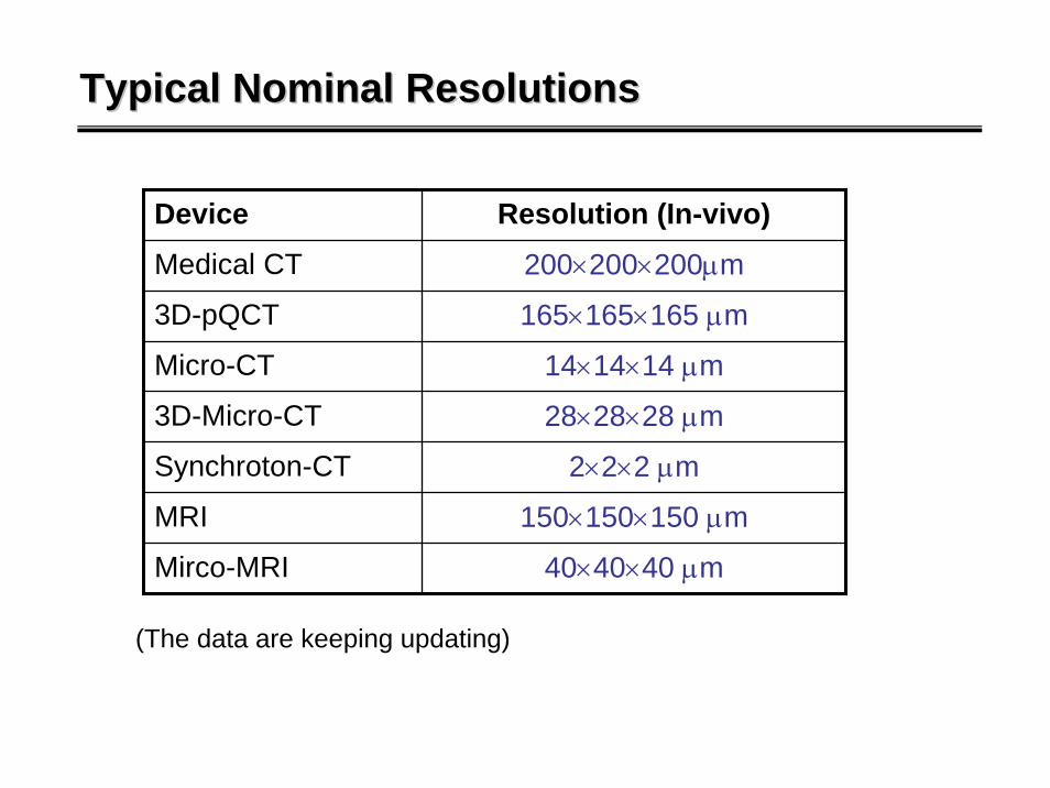
Typical Nominal ResolutionsTypical Nominal Resolutions

Device Resolution (In-vivo)Medical CT 200×200×200μm

3D-pQCT 165×165×165 μm

Micro-CT 14×14×14 μm

3D-Micro-CT 28×28×28 μm

Synchroton-CT 2×2×2 μm

MRI 150×150×150 μm

Mirco-MRI 40×40×40 μm

(The data are keeping updating)

DEXA DEXA –– Dual Energy XDual Energy X--ray ray AbsorptiometryAbsorptiometry

GE Lunar DEXA

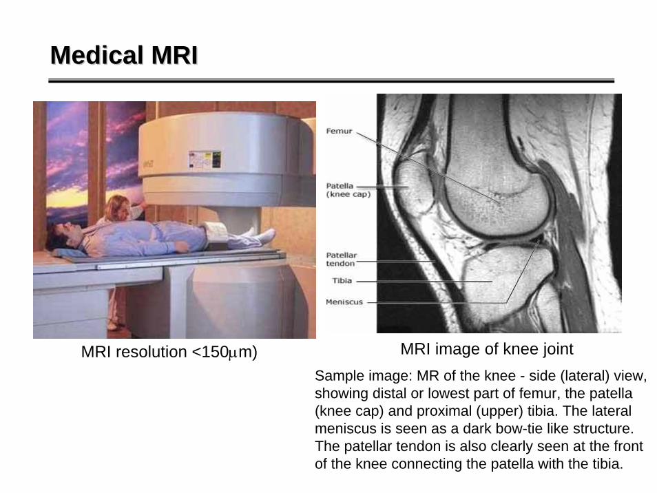
Medical MRIMedical MRI

MRI image of knee jointSample image: MR of the knee - side (lateral) view, showing distal or lowest part of femur, the patella (knee cap) and proximal (upper) tibia. The lateral meniscus is seen as a dark bow-tie like structure. The patellar tendon is also clearly seen at the front of the knee connecting the patella with the tibia.

MRI resolution <150μm)

MedicalMedical--CT ScanningCT Scanning

Medical CT Scanner (resolution <200μm)

MicroMicro--CT ScannerCT Scanner

MicroCT Scanner (SkyScan 1172, resolution <5μm)

Reconstruction: CT Scanning → sectional Image → Segmentation → 3D image (STL)

CT Reconstruction of Bone Microstructures CT Reconstruction of Bone Microstructures

32 years old man 59 years old man 89 years old man

37-year old man without bone disorder (lelf) and 73-year old osteoporotic woman (right)

Density and Density and EE--Modulus of Modulus of CancellousCancellous BoneBone

The best-established relationship is that between cancellous bone Young’s modulus and its structural apparent density (i.e. the weight per unit volume of a material including voids inherent ), as follows.

paE ρ=References Power Variance

Carter and Hayes (1977) J Bone Joint Surg, 59 :954 p=3.00 74%

Kabel et al (1999), Bone 24:115 p=1.93 94%

Rice et al (1988), J Biomech 21:155. p=2.00 78%

Hodgskinson and Currey (1992), J mater Sci Mater Med 3:377 p=1.96 94%

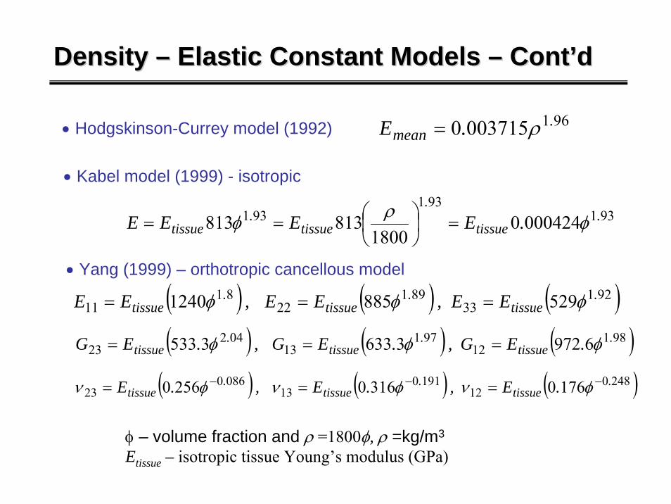
Density Density –– Elastic Constant Models Elastic Constant Models –– ContCont’’dd

931931

931 00042401800

813813 .tissue

.

tissue.

tissue .EEEE φρφ =⎟⎠⎞

⎜⎝⎛==

• Kabel model (1999) - isotropic

• Hodgskinson-Currey model (1992) 9610037150 .mean .E ρ=

( ) ( ) ( )92133

89122

8111 5298851240 .

tissue.

tissue.

tissue EE,EE,EE φφφ ===

( ) ( ) ( )98112

97113

04223 697236333533 .

tissue.

tissue.

tissue .EG,.EG,.EG φφφ ===

( ) ( ) ( )248012

191013

086023 176031602560 .

tissue.

tissue.

tissue .E,.E,.E −−− === φνφνφν

• Yang (1999) – orthotropic cancellous model

φ – volume fraction and ρ =1800φ, ρ =kg/m3

Etissue – isotropic tissue Young’s modulus (GPa)

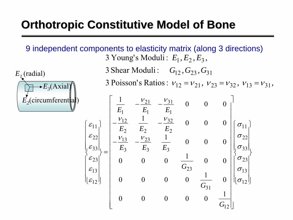
Orthotropic Constitutive Model of Bone Orthotropic Constitutive Model of Bone

9 independent components to elasticity matrix (along 3 directions)

⎪⎪⎪⎪

⎭

⎪⎪⎪⎪

⎬

⎫

⎪⎪⎪⎪

⎩

⎪⎪⎪⎪

⎨

⎧

⎥⎥⎥⎥⎥⎥⎥⎥⎥⎥⎥⎥⎥⎥⎥

⎦

⎤

⎢⎢⎢⎢⎢⎢⎢⎢⎢⎢⎢⎢⎢⎢⎢

⎣

⎡

−−

−−

−−

=

⎪⎪⎪⎪

⎭

⎪⎪⎪⎪

⎬

⎫

⎪⎪⎪⎪

⎩

⎪⎪⎪⎪

⎨

⎧

12

13

23

33

22

11

12

31

23

33

23

3

132

32

22

121

31

1

21

1

12

13

23

33

22

11

100000

010000

001000

0001

0001

0001

σσσσσσ

νν

νν

νν

εεεεεε

G

G

G

EEE

EEE

EEE

,,,G,G,G

,E,E,E

311332232112

312312

321

:RatiossPoisson'3:ModuliShear3

:ModulisYoung'3

νννννν ===E3(Axial)

E2(circumferential)

E1 (radial)

e3(Axial)

e2(circumferential)

e1 (radial)

Orthotropic Constitutive Model of Bone Orthotropic Constitutive Model of Bone –– ContCont’’d d

Young’s modulus Poisson’s ratio Shear modulus

E1=6.9GPa ν12=0.49, ν21=0.62 G12=2.41GPa

E2=8.5GPa ν13=0.12, ν31=0.32 G13=3.56GPa

E3=18.4GPa ν23=0.14, ν32=0.31 G23=4.91GPa

Young’s modulus Poisson’s ratio Shear modulus

E1=12.0GPa ν12=0.376, ν21=0.422 G12=4.53GPa

E2=13.4GPa ν13=0.222, ν31=0.371 G13=5.61GPa

E3=22.0GPa ν23=0.235, ν32=0.350 G23=6.23GPa

Tibia

Femur

(Humpherey and Delange, An introduction to Biomechanics, 2004)

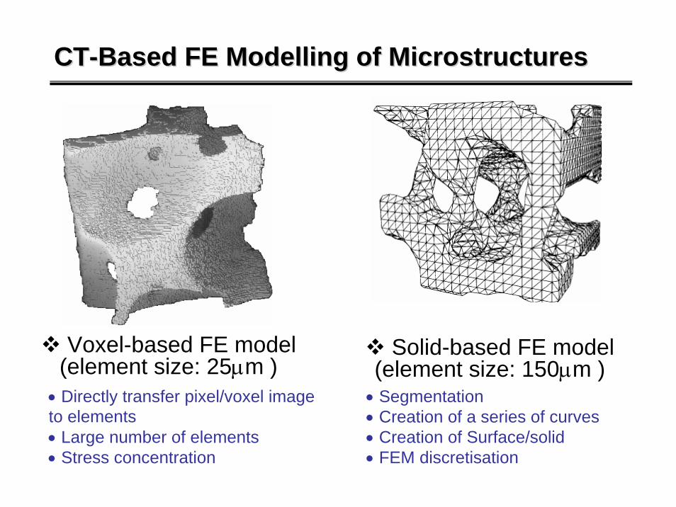
CTCT--Based FE Based FE ModellingModelling of Microstructuresof Microstructures

Voxel-based FE model(element size: 25μm )

Solid-based FE model(element size: 150μm )

• Directly transfer pixel/voxel image to elements• Large number of elements• Stress concentration

• Segmentation• Creation of a series of curves• Creation of Surface/solid• FEM discretisation

RemodelingRemodeling

Remodeling involves changes in biological material properties.

These changes, which often are adaptive, may be brought about by alterations in modulus, internal structure, strength, or density. For example, bones, and heart muscle may change their internal structures through reorientation of trabeculae and muscle fibers, respectively.

Wolff’s Law1892 Julius Wolff stated “every change in the function of bone is followed by certain definite changes in internal architecture and external conformation in accordance with mathematic laws.”

Cancellous Cortical

RemodellingRemodelling –– Biomechanical Causes Biomechanical Causes

Biological remodeling due to changes inBiological remodeling due to changes in•• Stress/strainStress/strain•• Strain energy densityStrain energy density•• Loading frequencyLoading frequency•• MicroMicro--crackscracks•• Temperature, environmentTemperature, environment

Remodeling (growth) of trees Remodeling (growth) of trees ((MattheckMattheck 1998)1998)

Bone remodeling in mice Bone remodeling in mice (Burr et al 2002)(Burr et al 2002)

RemodellingRemodelling –– Biomechanical Causes Biomechanical Causes

Step 1: stresses/strains cause a little crack, Step 2: cells turn into osteoclasts and dissolve (resorb) bone, Step 3: cells from the marrow space turn into osteoblasts and build new bone.

Remodeling mechanism due to microcracks

RemodellingRemodelling –– MicroMicro--cracks cracks

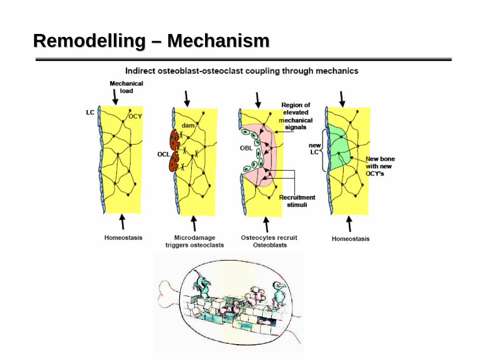
RemodellingRemodelling –– MechanismMechanism

Mechanical Stimuli Mechanical Stimuli -- ψψStrain energy density

Energy stress – linearise the quadratic nature of U

Mechanical intensity scalar (volumetric shrinking/swelling)

von Mises stress (σ1, σ2, σ3 – principal stresses)

{ } { } [ ]23231313121233332222111121

21 εσεσεσεσεσεσψ +++++=== εσ TU

UEavgenergy 2== σψ

( ) Usign 332211 εεεϑψ ++==

( ) ( ) ( )[ ]213

232

2212

1 σσσσσσσψ −+−+−== vm

Daily stress (ni = number of cycles of load case i, N=number of different load cases, m=exponent weighting impact of load cycles)

( ) mNi

miid n

1

1∑ === σσψ

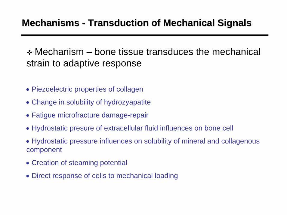
Mechanisms Mechanisms -- Transduction ofTransduction of Mechanical Mechanical SignalsSignals

Mechanism – bone tissue transduces the mechanical strain to adaptive response

• Piezoelectric properties of collagen

• Change in solubility of hydrozyapatite

• Fatigue microfracture damage-repair

• Hydrostatic presure of extracellular fluid influences on bone cell

• Hydrostatic pressure influences on solubility of mineral and collagenouscomponent

• Creation of steaming potential

• Direct response of cells to mechanical loading

Mechanical StimuliMechanical Stimuli -- ContCont’’dd

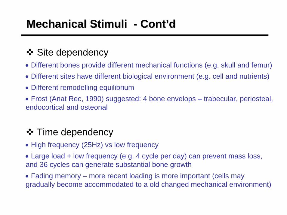
Site dependency• Different bones provide different mechanical functions (e.g. skull and femur)• Different sites have different biological environment (e.g. cell and nutrients)• Different remodelling equilibrium• Frost (Anat Rec, 1990) suggested: 4 bone envelops – trabecular, periosteal, endocortical and osteonal

Time dependency• High frequency (25Hz) vs low frequency• Large load + low frequency (e.g. 4 cycle per day) can prevent mass loss, and 36 cycles can generate substantial bone growth• Fading memory – more recent loading is more important (cells may gradually become accommodated to a old changed mechanical environment)

Model ClassificationModel Classification

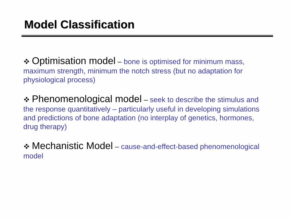
Optimisation model – bone is optimised for minimum mass, maximum strength, minimum the notch stress (but no adaptation for physiological process)

Phenomenological model – seek to describe the stimulus and the response quantitatively – particularly useful in developing simulations and predictions of bone adaptation (no interplay of genetics, hormones, drug therapy)

Mechanistic Model – cause-and-effect-based phenomenological model

RemodellingRemodelling

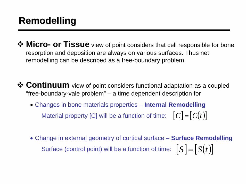
Micro- or Tissue view of point considers that cell responsible for bone resorption and deposition are always on various surfaces. Thus net remodelling can be described as a free-boundary problem

Continuum view of point considers functional adaptation as a coupled “free-boundary-vale problem” – a time dependent description for

• Changes in bone materials properties – Internal Remodelling

Material property [C] will be a function of time:

• Change in external geometry of cortical surface – Surface Remodelling

Surface (control point) will be a function of time:

[ ] ( )[ ]tCC =

[ ] ( )[ ]tSS =

Stimulus error:

Surface Surface RemodellingRemodelling RuleRule

( ) ( )t*te ψψ −=( ) stimulusmechanical=tψ

Surface Remodelling rate is proportional to stimulus error:(cs = constant)

Surface Remodelling Rule

ws = half-width of dead zone (lazy zone)

( ) ( )[ ]t*tcs s ψψ −=&

( ) ( )[ ] ( ) ( )( ) ( )

( ) ( )[ ] ( ) ( )⎪⎩

⎪⎨

⎧

−<−+−<−<−>−−−

=

sss

ss

sss

wt*twt*tcwt*tw

wt*twt*tcs

ψψψψψψψψψψ

forfor0

for&

Surface Surface RemodellingRemodelling RuleRule

*ψ ψ

Dead zoneLazy zone

0

s& ( ) ( )[ ]t*tcs s ψψ −=& ( ) ( )[ ]

( ) ( )[ ]⎪⎩

⎪⎨

⎧

+−

−−=

ss

ss

wt*tc

wt*tcs

ψψ

ψψ0&

sw* −ψ sw* +ψ

( ) ( )( ) ⎥

⎦

⎤⎢⎣

⎡ −=

t*t*tcs s ψ

ψψ&Alternative Remodel Rule

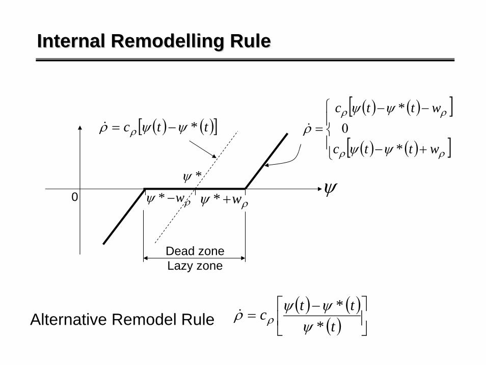
Internal Internal RemodellingRemodelling RuleRule

*ψ ψ

Dead zoneLazy zone

0

Alternative Remodel Rule

( ) ( )[ ]t*tc ψψρ ρ −=&( ) ( )[ ]

( ) ( )[ ]⎪⎩

⎪⎨

⎧

+−

−−=

ρρ

ρρ

ψψ

ψψρ

wt*tc

wt*tc0&

ρψ w* − ρψ w* +

( ) ( )( ) ⎥

⎦

⎤⎢⎣

⎡ −=

t*t*tc

ψψψρ ρ&

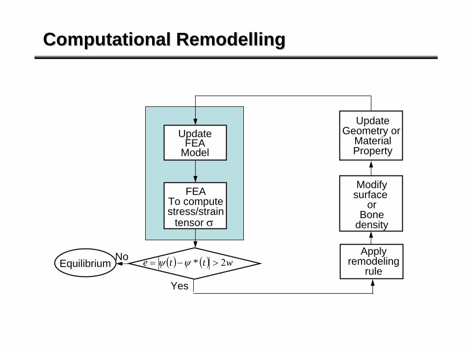
Computational Computational RemodellingRemodelling

Modifysurface

orBone

density

FEATo computestress/strain

tensor σ

UpdateFEA

Model

UpdateGeometry or

MaterialProperty

Applyremodeling

ruleYes

Equilibrium No ( ) ( ) wt*te 2>−= ψψ

Example 1 Example 1 –– Bone Loss in SpaceBone Loss in Space

Human spaceflight to mars could become a reality within the next 25 years, but not until some physiological problems are resolved, including an alarming loss of bone mass, fitness and muscle strength. Gravity at Mars' surface is about 38% of that on the earth. With lower gravitational forces, bones decrease in mass and density.

The rate at which we lose bone in space is 10-15 times greater than that of a postmenopausal woman and there is no evidence that bone loss ever slows in space. NASA has collected data that humans in space lose bone mass at a rate of c =1.5%/month so far.

Further, it is not clear that space travelers will regain that boneon returning to gravity. During a trip to mars, lasting between 13 and 30 months, unchecked bone loss could make an astronaut's skeleton the equivalent of a 100-year-old person.

Example Example –– Bone Loss in Space Bone Loss in Space –– ContCont’’dd

( ) ( )( ) ⎥

⎦

⎤⎢⎣

⎡ −=

−=≈=

+

t*t*tc

ttdtd nn

ψψψ

Δρρ

ΔρΔρρ ρ

1&

( ) ( )( ) tt*

t*tcnn Δψ

ψψρρ ρ ⎥⎦

⎤⎢⎣

⎡ −+=+1

Remodelling rule

380

MarstheonlevelStressearththeonlevelStress

.*

*

=

==

ψψψψ n%.c ρρ 51=

( ) ( )t.t%.. nnnn ΔρΔρρρ 009301516201 −=−=+Thus:

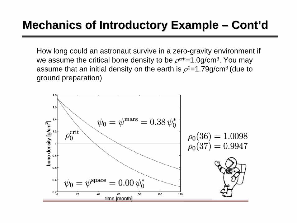
Mechanics of Introductory Example Mechanics of Introductory Example –– ContCont’’dd

How long could an astronaut survive in a zero-gravity environment if we assume the critical bone density to be ρcrit=1.0g/cm3. You may assume that an initial density on the earth is ρ0=1.79g/cm3 (due to ground preparation)

FS

S

x

y

l l

zF

Section S-S

x

y

Cortical

CancellousR

r

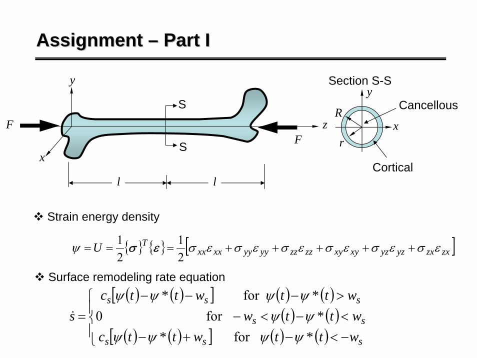
Assignment Assignment –– Part IPart I

{ } { } [ ]zxzxyzyzxyxyzzzzyyyyxxxxTU εσεσεσεσεσεσψ +++++===

21

21 εσ

Surface remodeling rate equation

Strain energy density

( ) ( )[ ] ( ) ( )( ) ( )

( ) ( )[ ] ( ) ( )⎪⎩

⎪⎨

⎧

−<−+−<−<−>−−−

=

sss

ss

sss

wt*twt*tcwt*tw

wt*twt*tcs

ψψψψψψψψψψ

forfor0

for&

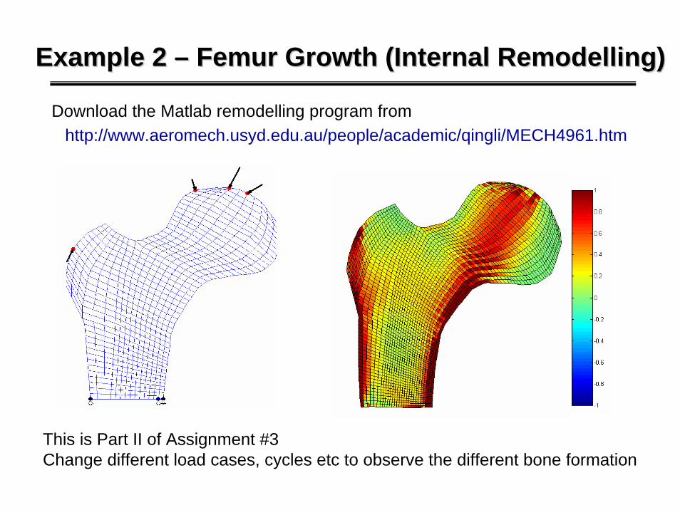
Example 2 Example 2 –– Femur Growth (Internal Femur Growth (Internal RemodellingRemodelling))

Download the Matlab remodelling program from http://www.aeromech.usyd.edu.au/people/academic/qingli/MECH4961.htm

This is Part II of Assignment #3Change different load cases, cycles etc to observe the different bone formation