
Lecture08(1)
21
BUS 105: Production and Operations Management © Mohsen ElHafsi 2014 BUS 105 Production/Operations Management Inventory Management Inventory Inventory can be visualized as stacks of money sitting on forklifts, on shelves, and in trucks and planes while in transit. For many businesses, inventory is the largest asset on the balance sheet at any given time. Inventory can be difficult to convert back into cash. It is a good idea to try to get your inventory down as far as possible. The average cost of inventory in the United States is 30 to 35 percent of its value. 2 Supply Chain Inventory Models 3
-
Upload
sriracha-luke -
Category
Documents
-
view
22 -
download
0
description
BUS 105 lecture
Transcript of Lecture08(1)

BUS 105: Production and Operations Management
© Mohsen ElHafsi 2014
BUS 105Production/Operations
Management
Inventory Management
Inventory Inventory can be visualized as stacks of money
sitting on forklifts, on shelves, and in trucks and planes while in transit.
For many businesses, inventory is the largest asset on the balance sheet at any given time.
Inventory can be difficult to convert back into cash.
It is a good idea to try to get your inventory down as far as possible. The average cost of inventory in the United States is
30 to 35 percent of its value.
2
Supply Chain Inventory Models
3

BUS 105: Production and Operations Management
© Mohsen ElHafsi 2014
Inventory Models
4
•Used when we are making a one-time purchase of an item
Single-period model
•Used when we want to maintain an item “in-stock,” and when we restock, a certain number of units must be ordered
Fixed-order quantity model
• Item is ordered at certain intervals of time
Fixed–time period model
Inventory: Definition & Types Inventory: the stock of any item or resource used
in an organization
Includes raw materials, finished products, component parts, supplies, and work-in-process
Manufacturing inventory: refers to items that contribute to or become part of a firm’s product
Replacement parts, tools, & supplies
Goods-in-transit to warehouses or customers
5
Inventory Systems The set of policies and controls that
monitor levels of inventory
Determines what levels should be maintained, when stock should be replenished, and how large orders should be
6

BUS 105: Production and Operations Management
© Mohsen ElHafsi 2014
Purposes of Inventory
7
To maintain independence of
operationsTo meet variation
in product demandTo allow flexibility
in production scheduling
To provide a safeguard for
variation in raw material delivery
time
To take advantage of economic
purchase order size
Inventory Costs
8
Holding (or carrying) costs•Costs for storage, handling,
insurance, and so on
Setup (or production change) costs•Costs for arranging specific
equipment setups, and so on
Ordering costs•Costs of placing an order
Shortage costs•Costs of running out
Costs
Demand Types
9
Independent demand – the demands for various items are unrelated to each other• For example, a workstation may
produce many parts that are unrelated but meet some external demand requirement
Dependent demand – the need for any one item is a direct result of the need for some other item• Usually a higher-level item of which
it is part
BUS 105: Production and Operations Management
© Mohsen ElHafsi 2014
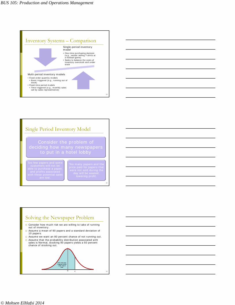
Inventory Systems – Comparison
10
Single-period inventory model• One-time purchasing decision
(e.g., vendor selling T-shirts at a football game)
• Seeks to balance the costs of inventory overstock and under stock
Multi-period inventory models• Fixed-order quantity models
• Event triggered (e.g., running out of stock)
• Fixed-time period models • Time triggered (e.g., monthly sales
call by sales representative)
Single Period Inventory Model
11
Consider the problem of deciding how many newspapers
to put in a hotel lobby
Too few papers and some customers will not be
able to purchase a paper, and profits associated
with these potential sales are lost.
Too many papers and the price paid for papers that were not sold during the
day will be wasted, lowering profit.
Solving the Newspaper Problem Consider how much risk we are willing to take of running
out of inventory. Assume a mean of 90 papers and a standard deviation of
10 papers. Assume we want an 80 percent chance of not running out. Assume that the probability distribution associated with
sales is Normal, stocking 90 papers yields a 50 percent chance of stocking out.
12

BUS 105: Production and Operations Management
© Mohsen ElHafsi 2014
Solving the Newspaper Problem From Appendix G, we see that we need
approximately 0.85 standard deviation of extra papers to be 80 percent sure of not stocking out. Using Excel, “=NORMSINV(0.8)” = 0.84162 Hence, the number of extra papers =
0.84162x10 = 9 papers (rounded)
13
Single-Period Inventory Models
14
cost per unit of demand over stocking level
cost per unit of demand under stocking level
probability that a given unit will be sold
u
o u
o
u
CP
C C
C
C
P
We should increase the size of the inventory so
long as the probability of selling the last unit
added is equal to or greater than the ratio ( )u o uC C C
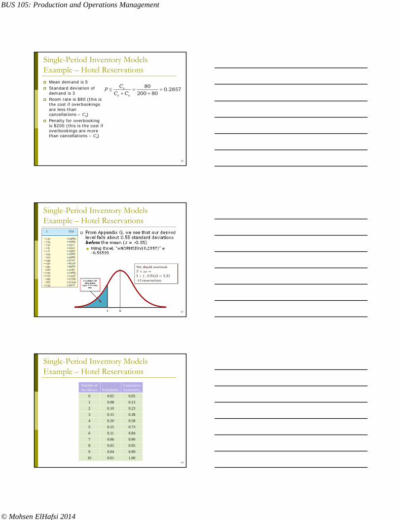
Single-Period Inventory ModelsExample – Hotel ReservationsA hotel near the university always fills up on the eveningbefore football games. History has shown that when the hotelis fully booked, the number of last-minute cancellations has amean of 5 and standard deviation of 3. The average room rateis $ 80. When the hotel is overbooked, the policy is to find aroom in a nearby hotel and to pay for the room for thecustomer. This usually costs the hotel approximately $200since rooms booked on such late notice are expensive. Howmany rooms should the hotel overbook?
15
BUS 105: Production and Operations Management
© Mohsen ElHafsi 2014
Single-Period Inventory ModelsExample – Hotel Reservations Mean demand is 5 Standard deviation of
demand is 3 Room rate is $80 (this is
the cost if overbookings are less than cancellations – Cu)
Penalty for overbooking is $200 (this is the cost if overbookings are more than cancellations – Co)
16
800.2857
200 80u
o u
CP
C C
Single-Period Inventory ModelsExample – Hotel Reservations
From Appendix G, we see that our desired level falls about 0.55 standard deviations below the mean (z = -0.55) Using Excel, “=NORMSINV(0.2857)” =
0.56599
17
Single-Period Inventory ModelsExample – Hotel Reservations
18
Number of No-Shows Probability
CumulativeProbability
0 0.05 0.05
1 0.08 0.13
2 0.10 0.23
3 0.15 0.38
4 0.20 0.58
5 0.15 0.73
6 0.11 0.84
7 0.06 0.90
8 0.05 0.95
9 0.04 0.99
10 0.01 1.00
BUS 105: Production and Operations Management
© Mohsen ElHafsi 2014
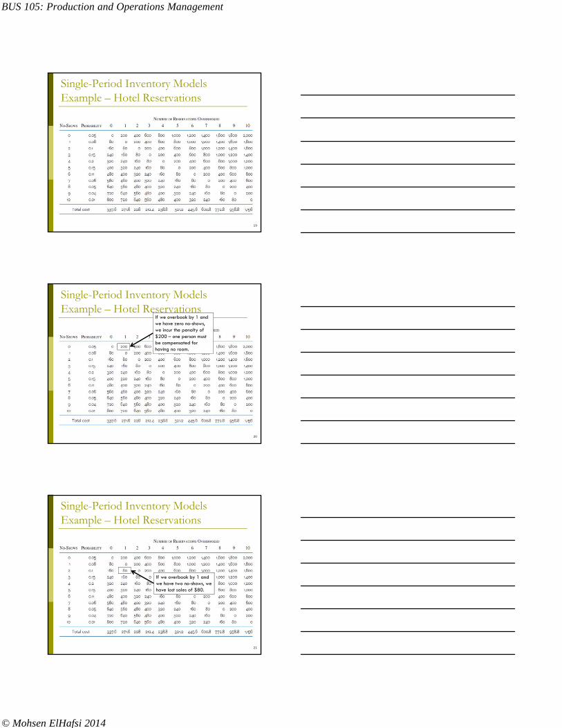
Single-Period Inventory ModelsExample – Hotel Reservations
19
Single-Period Inventory ModelsExample – Hotel Reservations
20
If we overbook by 1 and we have zero no-shows, we incur the penalty of $200 – one person must be compensated for having no room.
Single-Period Inventory ModelsExample – Hotel Reservations
21
If we overbook by 1 and we have two no-shows, we have lost sales of $80.

BUS 105: Production and Operations Management
© Mohsen ElHafsi 2014
Single-Period Inventory ModelsExample – Hotel Reservations
22
Total cost of a policy of overbooking by 9 rooms is the weighted average of the events (number of no-shows) and the outcome of those events.
Single Period Model Applications
23
Overbooking of airline flights
Ordering of clothing and other fashion items
One-time order for events – e.g., t-shirts for a concert
Multi-Period Models
24
Fixed-order quantity models- Also called the economic order quantity, EOQ, and Q-model
- Event triggered
Fixed–time period models- Also called the periodic system, periodic review system, fixed-order interval system, and P-
mode- Time triggered

BUS 105: Production and Operations Management
© Mohsen ElHafsi 2014
Multi-Period Models – Comparison
25
Inventory remaining must be continually monitored
Has a smaller average inventory
Favors more expensive items
Is more appropriate for important items
Requires more time to maintain – but is usually more automated
Is more expensive to implement
Counting takes place only at the end of the review period
Has a larger average inventory
Favors less expensive items
Is sufficient for less-important items
Requires less time to maintain
Is less expensive to implement
Fixed-Order Quantity Fixed-Time Period
Fixed-Order Quantity Models –Assumptions
Demand for the product is constant and uniform throughout the period.
Lead time (time from ordering to receipt) is constant.
Price per unit of product is constant. Inventory holding cost is based on
average inventory. Ordering or setup costs are constant. All demands for the product will be
satisfied.
26
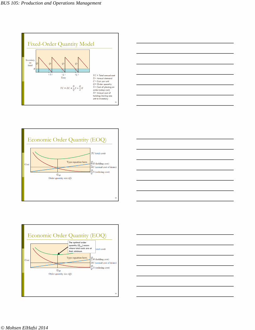
Fixed-Order Quantity Model
27

BUS 105: Production and Operations Management
© Mohsen ElHafsi 2014
Fixed-Order Quantity Model
28
Always order Q units when inventory reaches reorder point (R).
Fixed-Order Quantity Model
29
Inventory arrives after lead time (L). Inventory is raised to maximum level (Q).
Fixed-Order Quantity Model
30
Inventory is consumed at a constant rate, with a new order placed when the reorder point (R) is reached once again.
BUS 105: Production and Operations Management
© Mohsen ElHafsi 2014
Fixed-Order Quantity Model
31
Economic Order Quantity (EOQ)
32
Economic Order Quantity (EOQ)
33
The optimal order quantity (Qopt) occurs where total costs are at their minimum

BUS 105: Production and Operations Management
© Mohsen ElHafsi 2014
Economic Order Quantity (EOQ)
34
Economic Order Quantity (EOQ)Example: Problem Data
Annual Demand = 1,000 unitsDays per year considered in average daily demand
= 365Cost to place an order = $10Holding cost per unit per year = $2.50Lead time = 7 daysCost per unit = $15
Given the information below, what are the EOQ and reorder point?
35
Economic Order Quantity (EOQ)Example: Solution
2 2(1,000 )(10)* 89.443 90
2.50
DSQ units or units
H
1,000 /2.74 /
365 /
units yeard units day
days year
, 2.74 / (7 ) 19.18 20Reorder point R dL units day days or units
In summary, you place an optimal order of 90 units. In the course of using the units to meet demand, when you only have 20 units left, place the next order of 90 units.
36

BUS 105: Production and Operations Management
© Mohsen ElHafsi 2014
Economic Order Quantity (EOQ)Example: Problem Data
Annual Demand = 10,000 unitsDays per year considered in average daily demand = 365Cost to place an order = $10Holding cost per unit per year = 10% of cost per unitLead time = 10 daysCost per unit = $15
Determine the economic order quantity
and the reorder point given the following…
37
Economic Order Quantity (EOQ)Example: Problem Data
2 2(10,000 )(10)* 365.148 , 366
1.50
DSQ units or units
H
10,000 /27.397 /
365 /
units yeard units day
days year
27.397 / (10 ) 273.97 274R dL units day days or units
Place an order for 366 units. When in the course of using the inventory you are left with only 274 units, place the next order of 366 units.
38
Inventory Models with Price Break(Quantity Discount Models)
Under quantity discounts, a supplier offers a lower unit price if larger quantities are ordered at one time
This model differs from the basic EOQ Model because the purchasing cost (C) varies with the quantity ordered
39

BUS 105: Production and Operations Management
© Mohsen ElHafsi 2014
Inventory Models with Price Break Under this condition, purchasing cost
becomes an incremental cost and must be considered in the determination of the EOQ
If the holding cost is based on a percentage of the price (H=iC), then
TC = (Q/2)iC +(D/Q)S + (D)C
40
Inventory Models with Price BreakFinding The EOQ
For each discount price, compute the EOQ
For any discount price, if the EOQ falls out of range, adjust the EOQ upward to the lowest quantity that will qualify for the discount.
Compute the total cost associated with each EOQ (after adjustment)
Select the EOQ with the lowest cost. It will be the quantity that minimizes the total cost.
41
Inventory Models with Price-Break Example: Problem Data
A company has a chance to reduce their inventoryordering costs by placing larger quantity orders usingthe price-break order quantity schedule below. Whatshould their optimal order quantity be if thiscompany purchases this single inventory item withan e-mail ordering cost of $4, a carrying cost rate of2% of the inventory cost of the item, and an annualdemand of 10,000 units?Order Quantity (units) Price/unit($)
0 to 2,499 $1.202,500 to 3,999 $1.004,000 or more $0.98
42

BUS 105: Production and Operations Management
© Mohsen ElHafsi 2014
Price-Break Example: Solution
2(10,000)(4)* 1,826
0.02(1.20)Q units
Annual Demand (D)= 10,000 unitsCost to place an order (S)= $4
First, plug data into formula for each price-break value of “C”
2(10,000)(4)* 2,000
0.02(1.00)Q units
2(10,000)(4)* 2,020
0.02(0.98)Q s units
Carrying cost % of total cost (i)= 2%Cost per unit (C) = $1.20, $1.00, $0.98
Interval from 0 to 2499, the Q* value is feasible
Interval from 2500-3999, the Q* value is not feasible
Interval from 4000 & more, the Q* value is not feasible
Next, determine if the computed Q* values are feasible or not
43
Price-Break Example: Solution Since the feasible solution occurred in the first price-break, it means that all the other true Q* values occur at the beginnings of each price-break interval. Why?
0 1826 2500 4000 Order Quantity
Tota
l ann
ual c
ost
So the candidates for the price-breaks are 1826, 2500, and 4000 units
Because the total annual cost function is a “U” shaped function
44
Price-Break Example: Solution
2
D QTC DC S iC
Q
Next, we plug the true Q* values into the total annual cost function to determine the total cost under each price-break
TC(0-2499)=(10000*1.20)+(10000/1826)*4+(1826/2)(0.02*1.20)
= $12,043.82
TC(2500-3999)= $10,041
TC(4000&more)= $9,949.20
Finally, we select the least costly Qopt, which is this problem occurs in the 4000 & more interval. In summary, our optimal order quantity is 4000 units
45

BUS 105: Production and Operations Management
© Mohsen ElHafsi 2014
Establishing Safety Stock Levels
46
•Safety stock can be determined based on many different criteria.
Safety stock – refers to the amount of inventory carried in addition to expected demand.
A common approach is to simply keep a certain number of weeks of supply.
•Assume demand is normally distributed.•Assume we know mean and standard deviation.•To determine probability, we plot a normal distribution for expected demand and note where the amount we have lies on the curve.
A better approach is to use probability.
Fixed-Order Quantity Model with Safety Stock
In the fixed order quantity model, the ordering process is triggered when the inventory level drops to a critical point, the Reorder Point (ROP).
This starts the lead time for the item. Lead time is the time to complete all activities
associated with placing, filling and receiving the order.
During the lead time, customers continue to draw down the inventory
It is during this period that the inventory is vulnerable to stockout (run out of inventory)
47
Fixed-Order Quantity Model with Safety Stock Customer service level is defined as the
probability that a stockout will not occur during the lead time.
The reorder point is set based on the Demand During Lead Time and the desired customer service level
The amount of safety stock needed is based on the degree of uncertainty in the demand during the lead time and the customer service level desired
48

BUS 105: Production and Operations Management
© Mohsen ElHafsi 2014
Fixed-Order Quantity Model with Safety Stock
Assumptions Demand per day is normally distributed with mean
and standard deviation d
Lead time (L) is constant
The distribution of the demand during the lead time is normal with mean and standard deviation
49
d
dL d L
Fixed-Order Quantity Model with Safety Stock The customer service level is converted into a z
value using the normal distribution table Safety Stock:
Expected Demand During Lead Time:
Reorder Point:
2dR EDDLT SS dL z L( )
50
dLSS z z L
EDDLT dL
Fixed-Order Quantity Model with Safety Stock
51

BUS 105: Production and Operations Management
© Mohsen ElHafsi 2014
Fixed-Order Quantity Model with Safety Stock
52
Demand is variable, but follows a known distribution/
Fixed-Order Quantity Model with Safety Stock
53
After the reorder is placed, demand during the lead time may be higher than expected, consuming some (or all) of the safety stock/
Fixed-Order Quantity Model with Safety Stock
54
BUS 105: Production and Operations Management
© Mohsen ElHafsi 2014
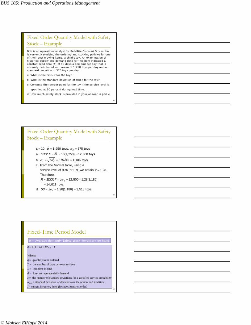
Fixed-Order Quantity Model with Safety Stock – ExampleBob is an operations analyst for Sell-Rite Discount Stores. He is currently studying the ordering and stocking policies for one of their best moving items, a child’s toy. An examination of historical supply and demand data for this item indicated a constant lead time (L) of 10 days a demand per day that is normally distributed with mean of 1,250 toys per day and a standard deviation of 375 toys per day.
a. What is the EDDLT for the toy?
b. What is the standard deviation of DDLT for the toy?
c. Compute the reorder point for the toy if the service level is
specified at 90 percent during lead time.
d. How much safety stock is provided in your answer in part c.
55
Fixed-Order Quantity Model with Safety Stock – Example
2
10, 1,250 toys, 375 toys
a. 10(1,250) 12,500 toys
b. 375 10 1,186 toys
c. From the Normal table, using a service level of 90% or 0.9, we obtain 1.28. Therefore,
12,50
d
L d
L
L d
EDDLT dL
L
z
R EDDLT z
0 1.28(1,186)
14,018 toys.d. 1.28(1,186) 1,518 toys.LSS z
56
Fixed-Time Period Model
( )
Where:
quantitiy to be ordered
the number of days between reviews
lead time in days
forecast average daily demand
the number of standard deviations for a specified service p
T Lq d T L z I
q
T
L
d
z
robability
= standard deviation of demand over the review and lead time
= current inventory level (includes items on order)T L
I
q = Average demand+Safety stock–Inventory on hand
57

BUS 105: Production and Operations Management
© Mohsen ElHafsi 2014
Fixed-Time Period Model
2
1
2
Since each day is independent and is constant,
( ) ( )
i
T L
T L di
d
T L d dT L T L
The standard deviation of a sequence of random events equals the square root of the sum of the variances
58
Fixed-Time Period Model – Example
Average daily demand for a product is 20 units.The review period is 30 days, and lead time is 10days. Management has set a policy of satisfying 96percent of demand from items in stock. At thebeginning of the review period there are 200 unitsin inventory. The daily demand standard deviationis 4 units.
Given the information below, how many units should be ordered?
59
Fixed-Time Period Model – Example
22( ) 30 10 4 25.298T L dT L
The value of z is found by using the Excel NORMSINV function, or using Appendix G and finding the value in the table that comes closest to the service probability.
So, from Appendix G, we have a probability of 0.9599, which is given by a z=1.75
60

BUS 105: Production and Operations Management
© Mohsen ElHafsi 2014
Fixed-Time Period Model – Example
( )
20(30 10) (1.75)(25.298) 200
800 44.272 200 644.272, 645
T Lq d T L z I
q
q or units
So, to satisfy 96 percent of the demand, you should place an order of 645 units at this review period
61
Assignment (7): February 26th, 2014
Read Chapter 20 Problems: 4, 5, 9,12, 14, 15, 21, 24, 26,
37 pp. 544-550
62