CS – 590.21 Analysis and Modeling of Brain Networks Department of Computer Science

University of Crete

Lecture on Temporal Correlation, Kolmogorov-Smirnov Test & K-means

Challenges in Quantifying Correlation

1. Correlated neurons fire at similar times but not precisely synchronously, so correlation must be defined with reference to a timescale within which spikes are considered correlated

2. Spiking is sparse with respect to the recording’s sampling frequency & spike duration

e.g., spiking rate 1 Hz, sampling rate typically 20 kHz (Demas et al., 2003)

This means that conventional approaches to correlation (such as Pearson’s correlation coefficient) are unsuitable

• as periods of quiescence should not count as correlated

• correlations should compare spike trains over short timescales, not just instantaneously.

Pearson Correlation

of two variables X & Y

(ρΧ,Υ)

Sample Pearson correlation coefficient

Datasets {x1,...,xn} & {y1,...,yn} containing n values

Pearson correlation: widely-used measure of the linear correlation between variables

No linear correlation

Positive linear correlation

Examples of Pearson Correlation

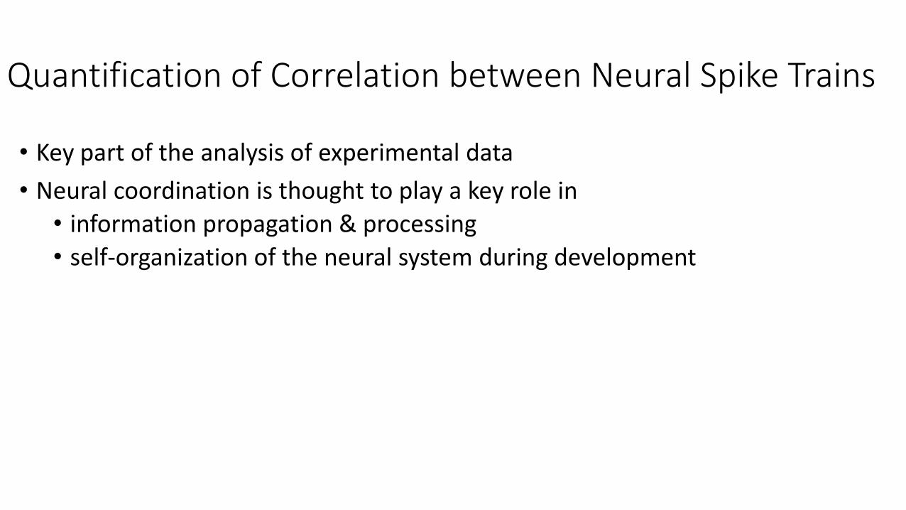
Quantification of Correlation between Neural Spike Trains

• Key part of the analysis of experimental data

• Neural coordination is thought to play a key role in

• information propagation & processing

• self-organization of the neural system during development

Designing the Appropriate Temporal Correlation Metric

• Symmetry

• Treatment of idle periods

• Robustness to variations in the firing rates

e.g., doubling the firing rate of two spike trains with a specific firing structure, does their correlation remain the same?

• Robust to the recording duration

• Bounded

• Distinction of the correlation vs. no correlation vs. anti-correlation

• Minimal assumptions on the underlying structure/distribution of the events

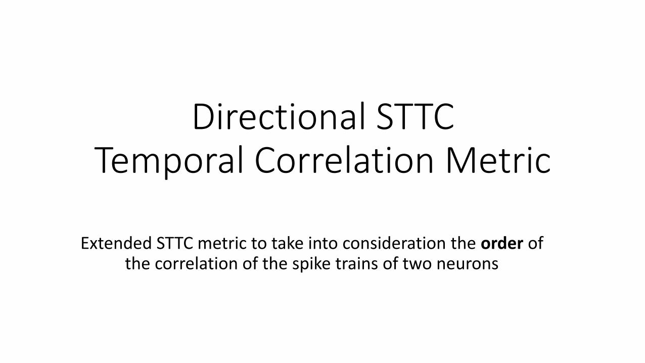
Directional STTC Temporal Correlation Metric

Extended STTC metric to take into consideration the order of the correlation of the spike trains of two neurons

Directional STTCAB represents a measure of the chance that firing events of A will precede firing events of B

Directional STTC Synchronous (lag = 0)

Spike trains of 100 time unit with uniform distr [ 10, 30 ] spikes 10,000 pairs

Advantages of Directional STTC

Relative spike-time shifts (lag parameter)

Order between neurons with respect to their firing events

Local fluctuations of neural activity or noise

• accounting the amount of correlation expected by chance

The presence of periods without firing events

• only the firing events contribute

CA

Conditional STTC (A->B |C) represents a measure of the chance that firing events of A will precede firing events of B, given the presence of firing of C

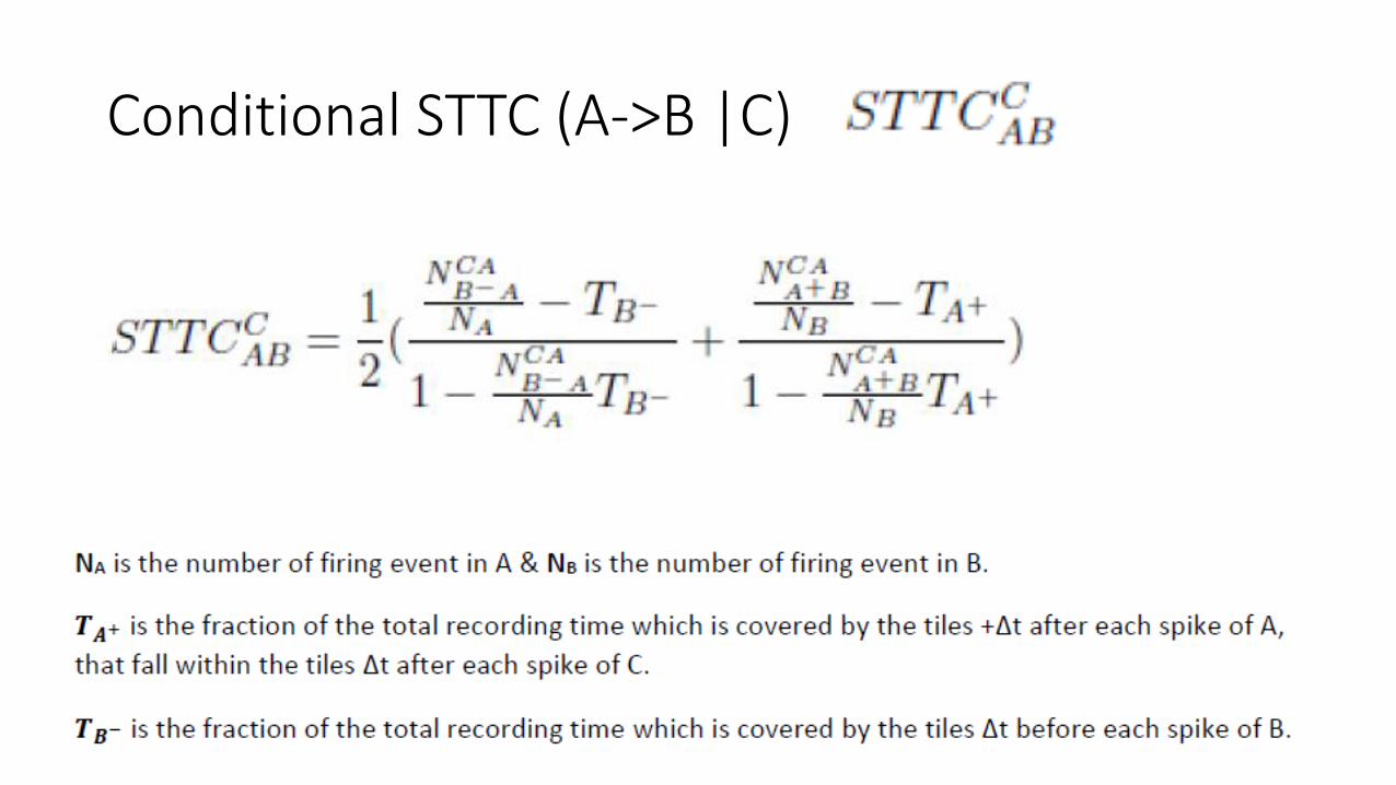
Conditional STTC (A->B |C)

“AB” indicates that firing events of A proceed firing events of B by a specific lag

Null distribution: STTC values for the circular shifted neurons (by random delays)

Significant Motifs Significant edge: real STTC value > 3 std. dev. of null distribution

Control (synthetic data) Each neuron trace is circular shifted by random delay For each pair of ‘shifted’ neurons, estimate the directional STTC & null distr. Identify the significant edges

Null distribution test for directional STTC

For a given pair (A,B) 1. Circular shift the spike train of the neuron A (generated spike train Ai ) 2. Estimate the directional STTC(Ai, B)

Repeat the above steps 100 times (i=1, … , 100) 3. Estimate the mean & standard deviation of the obtained STTC values 4. The statistical significant threshold (thr) = mean + 3 std dev

Criterion:

If the directional STTC (A, B) > thr , the directional STTC (A,B) is statistically significant.

The criterion can be strengthen with more repetitions (e.g., 1000), a larger number of std dev (e.g., 5).

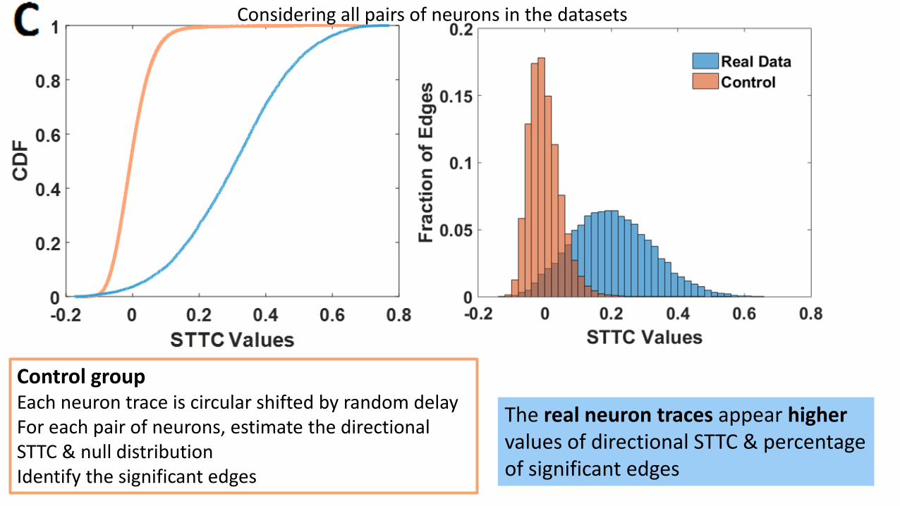
Control group Each neuron trace is circular shifted by random delay For each pair of neurons, estimate the directional STTC & null distribution Identify the significant edges

The real neuron traces appear higher values of directional STTC & percentage of significant edges

Considering all pairs of neurons in the datasets

Strengthen the Criterion of Significant Directional STTC (A,B)

Additional requirements

• The total number of spikes of A within a STTC lag of spikes of B is above 3.

• The total number of spikes of B within a STTC lag of spikes of A is above 3.

Kolmogorov-Smirnov (K-S) Test

• Non-parametric test of the equality of continuous 1D probability distributions • Quantifies a distance between two distribution functions • Can serve as a goodness of fit test

• Null hypothesis H0: Two samples drawn from populations with same distribution The maximum absolute difference between the two CDFs

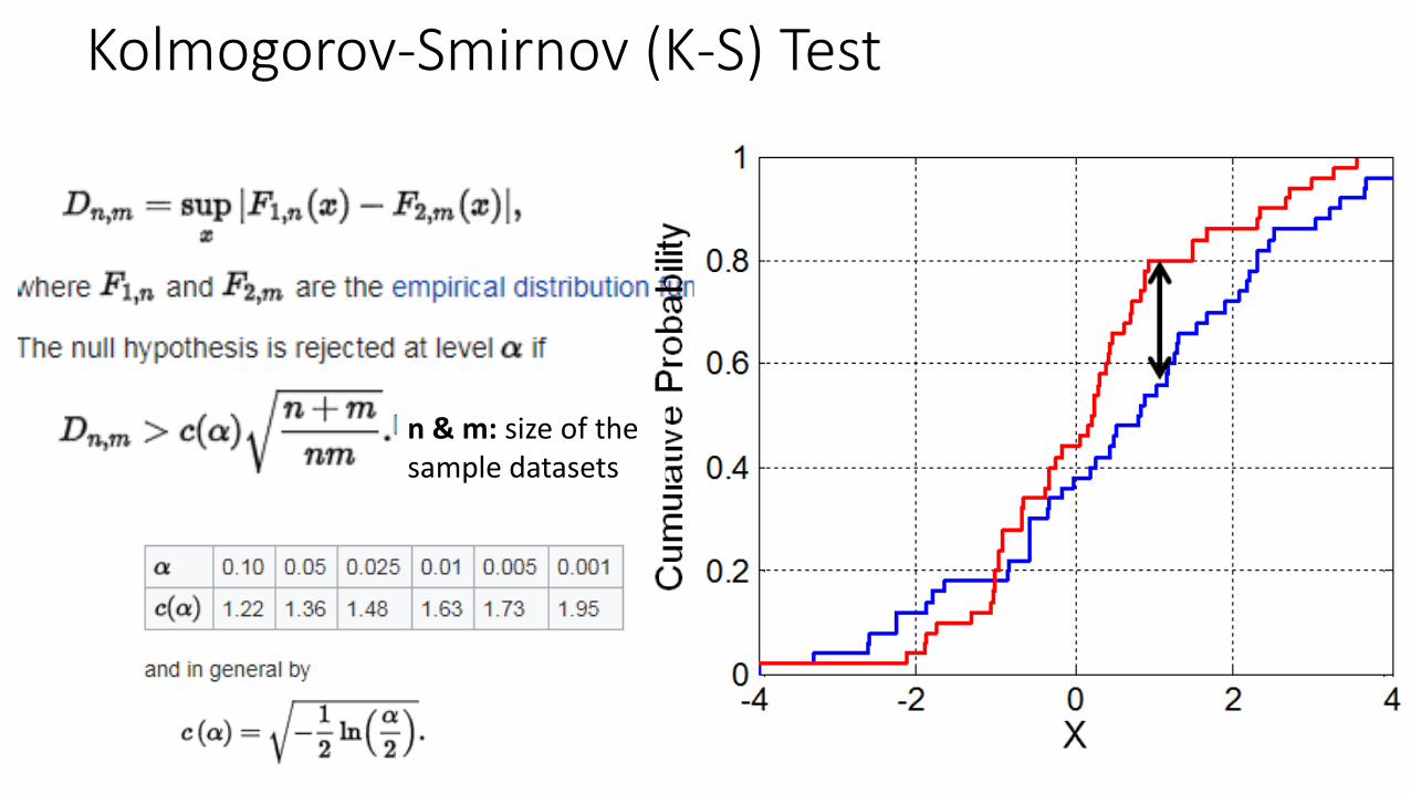
Kolmogorov-Smirnov (K-S) Test

n & m: size of the sample datasets

Kolmogorov-Smirnov (K-S) Test

Kolmogorov computed the expected distribution of the distance of the two CDFs when the null hypothesis is true.

Example: Kolmogorov-Smirnov Test

Decision p-value Distance Lag True Null Null Null True Null Null Null True Null Null Null 1 1 0 0 0.5427 0.79 0.0076 2 1 0 0 0.2126 0.78 0.0100 3 1 0 0 0.98485 0.75 0.0043 4 1 0 0 0.9937 0.72 0.0040 5 1 0 0 0.9769 0.68 0.00453

For all neuron pairs (A, B), populate the following distributions with Population 1: real STTC of the pair (A,B) Population 2: random circular shift in one of the two spike trains of (A,B) Population 3: random circular shift in one of the two spike trains of (A,B)

True Null: Population 1 vs. Population 2 Null Null: Population 2 vs. Polulation 3

Distance of two distributions in sup norm