lecture notes - Quantum Device Lab
219
Quantum Systems for Information Technology winter semester 06/07 Structure • introduction to quantum information processing – quantum mechanics reminder – qubits, qubit dynamics – entanglement, teleportation – Bell inequalities – measurement, decoherence – quantum algorithms (Deutsch-Jozsa, factoring, searching) • quantum systems for information technology – ions and neutral atoms in electromagnetic traps – nuclear magnetic resonance in molecules and solids – charges and spins in semiconductor quantum dots – charges and flux quanta in superconducting electronic circuits • selected topics of current research
Transcript of lecture notes - Quantum Device Lab

Quantum Systems for Information Technology
winter semester 06/07
Structure
• introduction to quantum information processing– quantum mechanics reminder
– qubits, qubit dynamics
– entanglement, teleportation
– Bell inequalities
– measurement, decoherence
– quantum algorithms (Deutsch-Jozsa, factoring, searching)
• quantum systems for information technology– ions and neutral atoms in electromagnetic traps
– nuclear magnetic resonance in molecules and solids
– charges and spins in semiconductor quantum dots
– charges and flux quanta in superconducting electronic circuits
• selected topics of current research

Guest Lectures
• ion trap quantum computing, Hartmut Haeffner, Innsbruck
• quantum dots
• nuclear spins
Time and Place
• lecture: Monday, 14:45 – 16:30, HCI D 2
• exercises: Tuesday, 13:45 – 14:30, HCI H 8
• are there timing conflicts with other lectures?

Credit Requirements
• attend lectures
• attend problem solving classes
• solve problem sets and present solutions to problems in class at least twice
• do a 25 minute presentation on a topic of current research in Quantum Information Science to the class.
• topics will be chosen from a selection of research papers to be made available later during the semester.
Exams
• Sessionspruefung (summer 2007)
• other dates possible for mobility students (contact your mobility program advisor)

Fire it up!

David Schuster, Andrew Houck, Blake Johnson, Joseph Schreier, Jay Gambetta, Jerry Chow, Hannes Majer, Luigi Frunzio,
Michel Devoret, Steven Girvin, and Rob Schoelkopf(Depts of Applied Physics and Physics, Yale University)
Alexandre Blais (Université de Sherbrooke, Canada) Johannes Fink, Martin Göppl, Romeo Bianchetti, Jonah Waissman, Peter Leek, Parisa Fallahi, Will Braff (ETH Zurich)
Quantum Optics andQuantum Information Processing
with Superconducting CircuitsAndreas Wallraff (ETH Zurich)

Quantum Electrical Circuits (Qubits)
Review: M. H. Devoret, A. Wallraff and J. M. Martinis,
condmat/0411172 (2004)
Non-Classical Features of Quantum Systems

Quantum Information Processing
M. Nielsen, I. Chuang, Quantum Computation and Quantum Information (Cambridge, 2000).
Realizations of Quantum Electrical Circuits
NEC, Japan
Nature 398(1999)
TU Delft, Netherlands
Science 285, 290, 299(1999, 2000, 2003)
CEA Saclay, France
Science 296 (2002)
NIST, UCSB
Phys. Rev. Lett. 89, 93(2002, 2004)
NEC, Japan
Nature 421, 425(2003, 2003)
recent review: G. Wendin and V.S. Shumeikocond-mat/0508729 (2005)
NIST, UCSB
Science 307(2005)

Cavity Quantum Electrodynamics (CQED)
D. Walls, G. Milburn, Quantum Optics (Spinger-Verlag, Berlin, 1994)
Motivation
A. Blais, R.-S. Huang, A. Wallraff, S. M. Girvin, and R. J. Schoelkopf,
PRA 69, 062320 (2004)

Circuit QED Architecture
A. Blais, R.-S. Huang, A. Wallraff, S. M. Girvin, and R. J. Schoelkopf,PRA 69, 062320 (2004)
elements
• the cavity: a superconducting 1D transmission line resonator (large E0)
• the artificial atom: a Cooper pair box (large d)
1D Transmission Line Cavity

The Cooper Pair Box
Realization
A. Wallraff, D. Schuster, ..., S. Girvin, and R. J. Schoelkopf,
Nature (London) 431, 162 (2004)

Qubit Measurement: Non-Resonant Interaction
A. Blais et al., PRA 69, 062320 (2004)
Time-Resolved Dispersive QND Readout
Wallraff, Schuster, Blais, ... Girvin, and Schoelkopf,
Phys. Rev. Lett. 95, 060501 (2005)

Varying the Control Pulse Length
Wallraff, Schuster, Blais, ... Girvin, and Schoelkopf, Phys. Rev. Lett. 95, 060501 (2005)
High Visibility Rabi Oscillations
A. Wallraff, D. I. Schuster, A. Blais, L. Frunzio, J. Majer,
S. M. Girvin, and R. J. Schoelkopf, Phys. Rev. Lett. 95, 060501 (2005)

Coupled Qubits
Coupled Qubit Device

Planned Operation of Two Qubit Gate (CNOT)
truth tableIN OUTqubit-qubit interaction (CNOT, XOR):
control qubit:
target qubit:
Circuit QED and Quantum Computation

New ETH Zurich Quantum Device Team
new lab started in April 2006

Quantum Systems for Information Technology
a brief introduction
A Brief Introduction
• classical information
• quantum information
• logic gates
• entanglement
• ‘no cloning theorem’
• teleportation
• quantum parallelism
• experimental realizations

basic unit of classical information: the bit
0 1
properties of a classical bit:
Classical Information
• easy to write
• easy to read out
• easy to copy
• extremely stable
single bit gate:
Classical Logic Gates
IN OUT
IN OUTNOT
NANDbit 1:
bit 2:
bit:
IN OUT
IN OUT
universal 2-bit gate:
irreversible

fundamental unit of quantum information
{ , }{0,1}qubit(quantum bit)
Quantum Information
superposition principle:
a + b a 0 + b 1
probability amplitudes
P(0) = |a|2, P(1) = |b|2
|a|2+|b|2 = 1
in basis state:
Measurement of a Qubit
a + b P( ) = |a|2
P( ) = |b|2
in superposition state:

preparation and measurement of the same property :
{ , } { , }e.g. polarization:
Measurement of different properties
preparation of one and measurement of a different property :
Probabilistic result: it is fundamentally impossible to predict outcome of all measurements with certainty
state of quantum object before measurement
superposition of states and
state of quantum object after measurement:
classical result or
Some strange properties of quantum objects

Generation of superposition states:
Rotate qubit by 90 degrees:
Quantum Logic Operation on a Single Qubit
qubit-qubit interaction (CNOT, XOR):
Quantum Logic Operation on Two Qubits: CNOT
CNOT truth table:
control qubit:
target qubit:
IN OUT

creation of superposition
on qubit 1
final state
Quantum Logic Circuit
qubit 1
qubit 2
CNOT
qubi
t1
qubi
t2
what is this final state
qubi
t1
qubi
t2BOBALICE
Alice’s measurement on her qubitdetermines the state of Bobs qubit ... instantaneously
Entanglement

a
b
Alice
teleportation of a quantum state
a
b
Bob
Features of Entanglement
what could entanglement be used for?
- a way for communicating an unknown quantum state- a resource for quantum information processing
the circuit:
A scheme for teleportation
a
b
a
b

Classical: 2n states for n classical bits
Quantum: simultaneous superposition of 2n states
acting on 1 qubit has effect on the n-1 other qubits
1) simulation of quantum systems; Feynman 1982
2) factoring; Shor 1994
3) searching; Grover 1996
Quantum Parallelism
Decoherence
superposition states are fragile: effect of the measurement
Required qubit properties:
Experimental Realization
• sensitive to external manipulation
• insensitive to rest of the world (environment)

Copying (Qu)bits
IN OUT
CNOTorig.
scratch
IN OUT
classical copying circuit CNOT
orig.
copy
a +ba +b
CNOT
CNOT
quantum version
=a +b
a +b a +b
?OK NO !
Copying qubits is impossible: No cloning theorem
• additional difficulty to deal with errors in quantum information
for basis states for superposition states

E
...
(non-linear)
Experimental Realizations: Ions in Traps
Josephson junction: non-linear inductance
~µm
Delft Delft IPHT
coherent collective properties of billions of electrons
Superconducting Qubits

• Quantum information has interesting additional features in comparison to classical information
• superposition of states
• entanglement
• Promises to speed-up some important information processing tasks
• Experimental realizations are under development• ion traps
• superconducting circuits
• semiconductor quantum dots
• nuclear spins
Summary
March, 1949 edition of Popular Mechanics
“I think there is a world market for about five computers”
"Where a calculator on the Eniac is equipped with 18,000 vacuum tubes and weighs 30 tons, computers in the future may have only 1,000 vacuum tubes and perhaps weigh 1-1/2 tons"
remark attributed to Thomas J. Watson (Chairman of the Board of IBM, 1943 )
Making predictions about the future can be difficult

We are optimistic …
Dilbert's take on Quantum Computers:
… but careful too.

Quantum Bits
a classical bit (Binary digIT) can take values either 0 or 1
realized as a voltage level in a digital circuit (CMOS, TTL)- 5 V = 1- 0 V = 0
a quantum bit can take values (quantum mechanical states)
in Dirac notation
Quantum bits (qubits) are quantum mechanical systems with two distinct quantum mechanical states. Qubits can be realized in a wide variety of physical systems displaying quantum mechanical properties. These include atoms, ions, electronic and nuclear magnetic moments, charges in quantum dots, charges and fluxes in superconducting circuits and many more. A suitable qubit should fulfill the DiVincenzo criteria (will be discussed in detail later).
or both of them at the same time, i.e. it can be in a superposition of states (discussed later).
Quantum Systems for Information Technology (QSIT) Page 1
inner product: is a function that takes two vectors from the Hilbert space and generates a complex number
QM postulate: The quantum state of an isolated physical system is completely described by its state vector in a complex vector space with a inner product (a Hilbert Space that is). The state vector is a unit vector in that space.
the qubit states are represented as vectors in a 2-dimensional Hilbert space (a complex vector space with inner product)
Quantum Systems for Information Technology (QSIT) Page 2

two state vectors are orthogonal when:
the norm of a state vector is:
definition of inner product on an n-dimensional Hilbert space
definition of the outer product:
Quantum Systems for Information Technology (QSIT) Page 3
Physical Realizations of Qubits
nuclear spins in molecules:
- solution of large number of molecules with nuclear spin
12 34
5
469.98 470.00 470.02 [MHz]
- distinct energies of different nuclei
- nuclear magnetic moment in external magnetic field
figures from MIT group (www.mit.edu/~ichuang/)
F
F13C12C
F
12CF
F13C
C5H5 (CO)2
FeFF
FF13C13C12C12C
FF
12C12CFF
FF13C13C
C5H5 (CO)2
FeFe
1
3
54
2
6
7
Quantum Systems for Information Technology (QSIT) Page 4

chain of ions in an ion trap:
qubit states are implemented as long lived electronic states of atoms
figures from Innsbruck group(http://heart-c704.uibk.ac.at/)
Quantum Systems for Information Technology (QSIT) Page 5
electrons in quantum dots:
200 nmML R
PL PR
IDOT
IQPCIQPC
GaAs/AlGaAs heterostructure2DEG 90 nm deepns = 2.9 x 1011 cm-2
GaAs/AlGaAs heterostructure2DEG 90 nm deepns = 2.9 x 1011 cm-2
GaAs/AlGaAs heterostructure2DEG 90 nm deepns = 2.9 x 1011 cm-2
- double quantum dot- control individual electrons
figures from Delft group(http://qt.tn.tudelft.nl/)
- spin states of electrons as qubit states- interaction with external magnetic field B
↑
↓B=0 B>0
gμBB↑
↓B=0 B>0
gμBB
Quantum Systems for Information Technology (QSIT) Page 6

superconducting circuits:
~µm~µm~µm
DelftDelft Delft IPHTDelftDelft IPHTIPHT
- circulating currents are qubit states
- made from sub-micron scale superconducting inductors and capacitors
- qubits made from circuit elements
Quantum Systems for Information Technology (QSIT) Page 7
polarization states of photons:
- qubit states corresponding to different polarizations of a single photon (in the visible frequency range)
- are used in quantum cryptography and for quantum communication
Quantum Systems for Information Technology (QSIT) Page 8

a qubit can be in a superposition of states
when the state of a qubit is measured one will find
where the normalization condition is
this just means that the sum over the probabilities of finding the qubit in any state must be unity
example:
Quantum Systems for Information Technology (QSIT) Page 9
Bloch Sphere Representation of Qubit State Space
alternative representation of qubit state vector
unit vector pointing at the surface of a sphere:
global phase factorazimuthal anglepolar angle
- any single qubit operation can be represented as a rotation on a Bloch sphere (see exercises)
- there is no generalization of Bloch sphere picture to many qubits
Quantum Systems for Information Technology (QSIT) Page 10

information content in a single qubit:
- infinite number of qubit states- but single measurement reveals only 0 or 1 with probabilities or - measurement will collapse state vector on basis state- to determine and an infinite number of measurements has to be made
But, if not measured qubit contains 'hidden' information about and
Quantum Systems for Information Technology (QSIT) Page 11
Single Qubit Gates
quantum circuit for a single qubit gate operation:
operations on single qubits:
bit flip
bit flip*
phase flip
identity
Quantum Systems for Information Technology (QSIT) Page 12

Pauli Matrices
The action of the single qubit gates discussed before can be represented by Pauli matrices acting on the computational basis states:
bit flip (NOT gate)
bit flip*(with extra phase)
phase flip
identity
all are unitary:
exercise: calculate eigenvalues and eigenvectors of all Pauli matrices and represent them on the Bloch sphere
Quantum Systems for Information Technology (QSIT) Page 13
Hadamard gate:
generates superpositions of single qubit states
matrix representation of Hadamard gate:
exercise: write down the action of the Hadamard gate on the computational basis states of a qubit.
Quantum Systems for Information Technology (QSIT) Page 14

Control of Qubit States
by resonant irradiation:
using a pulse of radiation with controlled frequency amplitude and length
preparation of a superposition state:assume the qubit to be in its ground state initially
assume a pulse of length will excite the qubit to state
then a pulse of length will bring the qubit to state
in fact such a pulse of chosen length and phase can prepare any single qubit state, i.e. any point on the Bloch sphere can be reached
Quantum Systems for Information Technology (QSIT) Page 15
QM postulate: The time evolution of a state ψ of a closed quantum system is described by a Schrödinger equation
where H is the hermitian operator known as the Hamiltonian describing the closed system.
the Hamiltonian:- H is hermitian and has a spectral decomposition- with eigenvalues E- and eigenvectors |E>- smallest value of E is the ground state energy with
the eigenstate |E>
general solution:
Dynamics of a Quantum System:
a closed quantum system does not interact with any other system
Quantum Systems for Information Technology (QSIT) Page 16

example:
on the Bloch sphere:
this is a rotation around the equator with Larmor precession frequency ω
e.g. electron spin in a field:
Quantum Systems for Information Technology (QSIT) Page 17
QM postulate: The evolution of a closed quantum system is described by a unitary transformation U. That is the state is related to the state by a unitary operator that only depends on
unitary operator (unitary matrix):
a unitary operator is a normal and hermitian operator
hermitian conjugate
generalized version:
connection with Schroedinger equation:- for any hermitian operator K the operator exp(iK) is unitary
Quantum Systems for Information Technology (QSIT) Page 18

normal operator:
hermitian operator:
properties of unitary operators:- preserve inner products- have a spectral decomposition
are eigenvalues of Uare eigenvectors of U
Quantum Systems for Information Technology (QSIT) Page 19
Rotation operators:
when exponentiated the Pauli matrices give rise to rotation matrices around the three orthogonal axis in 3-dimensional space.
If the Pauli matrices X, Y or Z are present in the Hamiltonian of a system they will give rise to rotations of the qubit state vector around the respective axis.
exercise: convince yourself that the operators Rx,y,z do perform rotations on the qubit state written in the Bloch sphere representation.
Quantum Systems for Information Technology (QSIT) Page 20

Quantum Measurement
One way to determine the state of a qubit is to measure the projection of its state vector along a given axis, say the z-axis.
On the Bloch spehere this corresponds to the following operation:
After a projective measurement is completed the qubit will be in either one of its computational basis states.
In a repeated measurement the projected state will be measured with certainty.
Quantum Systems for Information Technology (QSIT) Page 21
QM postulate: quantum measurement is described by a set of operators {Mm} acting on the state space of the system. The probability p of a measurement result m occurring when the state ψ is measured is
the state of the system after the measurement is
completeness: the sum over all measurement outcomes has to be unity
example: projective measurement of a qubit in state ψ in its computational basis
Quantum Systems for Information Technology (QSIT) Page 22

measurement operators:
measurement probabilities:
state after measurement:
measuring the state again after a first measurement yields the same state as the initial measurement with unit probability
Quantum Systems for Information Technology (QSIT) Page 23
Two Qubits:
2 classical bits with states: 2 qubits with quantum states:
- 2n different states (here n=2)- but only one is realized at
any given time
2n complex coefficients describe quantum state
normalization condition
- 2n basis states (n=2)- can be realized simultaneously - quantum parallelism
Quantum Systems for Information Technology (QSIT) Page 24

Composite quantum systems
QM postulate: The state space of a composite systems is the tensor product of the state spaces of the component physical systems. If the component systems have states ψi the composite system state is
example:
exercise: Write down the state vector (matrix representation) of two qubits, i.e. the tensor product, in the computational basis. Write down the basis vectors of the composite system.
This is a product state of the individual systems.
Quantum Systems for Information Technology (QSIT) Page 25
Information content in multiple qubits
- 2n complex coefficients describe state of a composite quantum system with n qubits!
- Imagine to have 500 qubits, then 2500 complex coefficients describe their state.
- How to store this state. 2500 is larger than the number of atoms in the universe. It is impossible in classical bits. This is also why it is hard to simulate quantum systems on classical computers.
- A quantum computer would be much more efficient than a classical computer at simulating quantum systems.
- Make use of the information that can be stored in qubits for quantum information processing!
Quantum Systems for Information Technology (QSIT) Page 26

Operators on composite systems:
Let A and B be operators on the component systems described by state vectors |a> and |b>. Then the operator acting on the composite system is written as
tensor product in matrix representation (example for 2D Hilbert spaces):
Quantum Systems for Information Technology (QSIT) Page 27
Entanglement:
Definition: An entangled state of a composite system is a state that cannot be written as a product state of the component systems.
example: an entangled 2-qubit state (one of the Bell states)
What is special about this state? Try to write it as a product state!
It is not possible! This state is special, it is entangled!
Quantum Systems for Information Technology (QSIT) Page 28

Measurement of single qubits in an entangled state:
measurement of first qubit:
post measurement state:
measurement of qubit two will then result with certainty in the same result:
The two measurement results are correlated! Correlations in quantum systems can be stronger than correlations in classical systems. This can be generally proven using the Bell inequalities which will be discussed later. Make use of such correlations as a resource for information processing, for example in super dense coding and teleportation.
Quantum Systems for Information Technology (QSIT) Page 29
Super Dense Coding
task: Try to transmit two bits of classical information between you (Bob) and your friend Alice (A) using only one qubit. (As you are living in a quantum world you areallowed to use on pair of entangled qubits that you have prepared ahead of time.)
protocol: A) Alice and Bob each have one qubit of an entangled pair in their possession
B) Bob does a quantum operation on his qubit depending on which 2 classical bits he wants to communicateC) Bob sends his qubit to AliceD) Alice does one measurement on the entangled pair
shared entanglement
local operations
send Bobs qubit to Alice
Alice measures
Quantum Systems for Information Technology (QSIT) Page 30

bits to be transferred:
Bobsoperation
resulting 2-qubit state Alice'soperation
measurein Bellbasis
- all these states are entangled (try!)- they are called the Bell states
comments:- two qubits are involved in protocol BUT Bob only interacts with one and sends only one
along his quantum communications channel- two bits cannot be communicated sending a single classical bit along a classical
communications channel
Quantum Systems for Information Technology (QSIT) Page 31
proposal of super dense coding and experimental demonstration using photons:
Communication via one- and two-particle operators on Einstein-Podolsky-Rosen statesPhys. Rev. Lett.69, 2881(1992)Charles H. Bennett and Stephen J. Wiesner
Dense coding in experimental quantum communicationPhys. Rev. Lett.76, 4656 (1996)Klaus Mattle, Harald Weinfurter, Paul G. Kwiat, and Anton Zeilinger
state manipulationBell state measurement
sym.
asym.
H = horizontal polarizationV = vertical polarization
Quantum Systems for Information Technology (QSIT) Page 32

Parametric Down Conversion:a source of polarization entangled photon pairs
Quantum Systems for Information Technology (QSIT) Page 33
Classical Logic Gates:
non trivial single bit logic gate: NOT
IN OUT
universal two bit logic gate: NANDAND followed by NOT
Other gates exist (AND, OR, XOR, NOR) but can all be implemented using NAND gates.
universality of NAND: Any function operating on bits can be computed using NAND gates. Therefore NAND is called a universal gate.
Quantum Systems for Information Technology (QSIT) Page 34

Two Qubit Quantum Logic Gates
The controlled NOT gate (CNOT):
function:
CNOT circuit:
addition mod 2 of basis states
comparison with classical gates:- XOR is not reversible- CNOT is reversible (unitary)
control qubit
target qubit
Universality of controlled NOT:Any multi qubit logic gate can be composed of CNOT gates and single qubit gates X,Y,Z.
Quantum Systems for Information Technology (QSIT) Page 35
application of CNOT: generation of entangled states (Bell states):
exercise: Write down the unitary matrix representations of the CNOT in the computational basis with qubit 1 being the control qubit. Write down the matrix in the same basis with qubit 2 being the control bit.
Quantum Systems for Information Technology (QSIT) Page 36

Quantum Teleportation:
Task: Alice wants to transfer an unknown quantum state ψ to Bob only using one entangled pair of qubits and classical information as a resource.
note: - Alice does not know the state to be transmitted- Even if she knew it the classical amount of information that she would need to send would be infinite.
The teleportation circuit:
Teleporting an unknown quantum state via dual classical and Einstein-Podolsky-Rosen channelsCharles H. Bennett, Gilles Brassard, Claude Crépeau, Richard Jozsa, Asher Peres, and William K. WoottersPhys. Rev. Lett. 70, 1895 (1993) [PROLA Link]
original article:
Quantum Systems for Information Technology (QSIT) Page 37
How does it work?
measurement of qubit 1 and 2, classical information transfer and single bit manipulation on target qubit 3:
Hadamard on qubit to be teleported:
CNOT between qubit to be teleported and one bit of the entangled pair:
Quantum Systems for Information Technology (QSIT) Page 38

(One) Experimental Realization of Teleportation using Photon Polarization:
- parametric down conversion (PDC) source of entangled photons- qubits are polarization encoded
Experimental quantum teleportation Dik Bouwmeester, Jian-Wei Pan, Klaus Mattle, Manfred Eibl, Harald Weinfurter, Anton ZeilingerNature 390, 575 - 579 (11 Dec 1997) Article Abstract | Full Text | PDF | Rights and permissions | Save this link
Quantum Systems for Information Technology (QSIT) Page 39
- polarizing beam splitters (PBS) as detectors of teleported states
Experimental Implementation
start with states
combine photon to be teleported (1) and one photon of entangled pair (2) on a 50/50 beam splitter (BS) and measure (at Alice) resulting state in Bell basis.
analyze resulting teleported state of photon (3) using polarizing beam splitters (PBS) single photon detectors
Quantum Systems for Information Technology (QSIT) Page 40

Experimental Realization of Teleporting an Unknown Pure Quantum State via Dual Classical and Einstein-Podolsky-Rosen ChannelsD. Boschi, S. Branca, F. De Martini, L. Hardy, and S. PopescuPhys. Rev. Lett. 80, 1121 (1998) [PROLA Link]
Unconditional Quantum TeleportationA. Furusawa, J. L. Sørensen, S. L. Braunstein, C. A. Fuchs, H. J. Kimble, and E. S. PolzikScience 23 October 1998 282: 706-709 [DOI: 10.1126/science.282.5389.706] (in Research Articles)Abstract » Full Text » PDF »
Complete quantum teleportation using nuclear magnetic resonance M. A. Nielsen, E. Knill, R. LaflammeNature 396, 52 - 55 (05 Nov 1998) Letters to Editor Abstract | Full Text | PDF | Rights and permissions | Save this link
Deterministic quantum teleportation of atomic qubits M. D. Barrett, J. Chiaverini, T. Schaetz, J. Britton, W. M. Itano, J. D. Jost, E. Knill, C. Langer, D. Leibfried, R. Ozeri, D. J. WinelandNature 429, 737 - 739 (17 Jun 2004) Letters to Editor Abstract | Full Text | PDF | Rights and permissions | Save this link
Deterministic quantum teleportation with atoms M. Riebe, H. Häffner, C. F. Roos, W. Hänsel, J. Benhelm, G. P. T. Lancaster, T. W. Körber, C. Becher, F. Schmidt-Kaler, D. F. V. James, R. BlattNature 429, 734 - 737 (17 Jun 2004) Letters to Editor Abstract | Full Text | PDF | Rights and permissions | Save this link
Quantum teleportation between light and matter Jacob F. Sherson, Hanna Krauter, Rasmus K. Olsson, Brian Julsgaard, Klemens Hammerer, Ignacio Cirac, Eugene S. PolzikNature 443, 557 - 560 (05 Oct 2006) Letters to Editor Full Text | PDF | Rights and permissions | Save this link
teleportation papers for you to present:
Quantum Systems for Information Technology (QSIT) Page 41

John Bell's thought experiment
- Charlie simultaneously prepares two particles having physical properties Q, R, S, T and gives one particle each to Alice and Bob.
- Alice measures the properties Q and R of her particle with the possible outcomes q = ±1 and r = ±1.
- Bob simultaneously measures the properties S and T of his particles with the possible outcomes s = ±1 and t = ±1.
consider the quantity:
the probability of the system being in state
is given by :
we also denote E(x) as the mean of the quantity x
Now, Alice and Bob perform measurements on the two particles and record their outcomes. Then they meet up and perform the multiplications (e.g. q s) and calculate the average values E(QS).
QSIT lecture II Page 1
What are the possible outcomes of measuring the quantity E(QS+RS+RT-QT)?
find an upper bound:
also:
Bell inequality
QSIT lecture II Page 2

measure this quantity for a Bell state:
Alice measures: Bob measures:
determine expectation values of joint measurements:
Bell states maximally violate the Bell inequality!
determine value of Bell inequality:
QSIT lecture II Page 3
Experimental violation of Bell Inequality (Alain Aspect):
Experimental Realization of Einstein-Podolsky-Rosen-BohmGedankenexperiment: A New Violation of Bell's InequalitiesA. Aspect, P. Grangier, and G. Roger Phys. Rev. Lett. 49, 91-94 (1982)[PDF (682 kB)]
Experimental Tests of Realistic Local Theories via Bell's TheoremA. Aspect, P. Grangier, and G. Roger Phys. Rev. Lett. 47, 460-463 (1981)
[PDF (665 kB)]
generation of polarization entangled photons:
setup:
measure coincidences and calculate correlation coefficient:
if (a,b)=0 (parallel polarizers) then E(a,b) = 1, i.e. perfect correlation of results
QSIT lecture II Page 4

quantum mechanical prediction:
for any γ
probability of individual photon measurements
probabilities of joint measurements on both photons:
easy to see for γ = 0
QSIT lecture II Page 5
experimental result:
repeat for different angles between polarizer (a,b) = θ:
measure Bell inequality:
with:
= 22.5 deg
QSIT lecture II Page 6

comments:
Consequences of violation of Bell inequalities:- The assumption that physical properties (e.g. Q, R, S, T) of systems have values which
exists independent of observation (the Realism Assumption) is wrong.- The assumption that experiments performed at one point in time and space (at Alices) cannot
be influenced by experiments at another point in time and space (at Bobs, in a different light cone) (the Locality Assumption) is wrong.
Both of the above assumptions are sometimes called Local Realism.
Quantum mechanics violates these assumptions, as shown in experiments!
Test of Locality: The Innsbruck Experiment
Violation of Bell's Inequality under Strict Einstein Locality ConditionsG. Weihs, T. Jennewein, C. Simon, H. Weinfurter, and A. Zeilinger Phys. Rev. Lett. 81, 5039-5043 (1998)[PDF (195 kB)]
QSIT lecture II Page 7
Reversible Classical Logic Gates
reversible computation: No information is ever erased. The input can always be reconstructed from the output
consequence: Reversible computation (e.g. quantum computation) can (in principle) be done without energy dissipation. (However, you may have to reset your memory at some point dissipating energy. Or you may perform a read-out (measurement) of the result of the computation that may dissipate energy. )
irreversible computation: Information is erased. E.g. in the standard AND gate the input bits are lost and cannot be reconstructed from the output.
Landauer's Principle: When a computer erases a single bit of information the amount of energy dissipated in the environment is at least kB T ln 2, where kB is the Boltzmann constant and T is the temperature of the environment. (Equivalent statement: When a computer erases a single bit of information the entropy of the environment increases by at least kB ln 2.)
note: Today's computers dissipate about 500 kB T ln 2 per elementary logic operation.
QSIT lecture II Page 8

The Toffoli gate
circuit representation:
truth table:flip target bit c if and only if control bits a and b are 1.
abc a'b'c'000 000001 001010 010011 011100 100101 101110 111111 110
control
target
properties:- this gate is reversible- it can be used to simulate classical NAND and FANOUT gates in a reversible way- an arbitrary circuit can be simulated efficiently using Toffoli gates
QSIT lecture II Page 9
Simulation of NAND
Simulation of FANOUT
Simulating classical gates using the Toffoli gate and ancilla bits (but possibly leaving some unused garbage bits behind)
QSIT lecture II Page 10

The Fredkin Gate
is a universal and reversible logic gate
truth table:swap target bits a and b if control bit c is 1.
abc a'b'c'000 000001 001010 010011 101100 100101 011110 110111 111
Simulating classical logic gates reversibly:
AND NOT CROSSOVER
this gate is conservative, i.e. the number of 1s at the input and output are conserved
QSIT lecture II Page 11
properties:- ancilla bits prepared in special states (0, 1) are allowed at input- extraneous (garbage) bits remain at output
Make use of classical NOT and CNOT gates to start out with all ancilla bits in state 0 and to reset extraneous states to some standard state that does not depend on the input after the function evaluation.
general function evaluation
garbage bitsevaluated function
remember: Classical version of CNOT can be used to copy classical bits from control to target state if target state is initialized to 0.
How to control the states of ancilla bits? How to avoid that the final state of some ancilla bits contain information that depends on the input state of the system? (The availability of such information will destroy quantum interference effects that we want to use for quantum information processing.)
QSIT lecture II Page 12

constructing a reversible version of the function f:
make a copy of input bit string x:
initial state:
inputoutput
ancillas
compute f:
bitwise addition of f(x) to y using CNOT:
run f backwards (it is reversible):
simplified expression (omit ancillas)
expression for general reversible function evaluation:
QSIT lecture II Page 13
Quantum Function Evaluation
example: function f acting on one bit
quantum version of function:
circuit for evaluating f:
simultaneous evaluation off(0) and f(1):
note:- A single circuit evaluating f once does so simultaneously for x = 0, 1 making use of
superposition states.- However, upon measurement one can only extract the result of one of the evaluations.
QSIT lecture II Page 14

generalization to many qubits:
preparation of superposition statefor all input data qubits using Hadamard gates
preparation of target qubit in |0>
result of functionevaluation
QSIT lecture II Page 15
Deutsch's Problem:
evaluate if a function f is constant or balanced
classically two queries of the function fare required to determine if it is constant or balanced.
Is there a more efficient way to solve Deutsch's problem on a quantum computer?Yes! Make use of superposition principle and quantum function evaluation!
Quantum Theory, the Church-Turing Principle and the Universal Quantum ComputerD. DeutschProceedings of the Royal Society of London. Series A, Mathematical and Physical Sciences > Vol. 400, No. 1818 (Jul., 1985), pp. 97-117 Article Information | Page of First Match | Print | Download
Rapid Solution of Problems by Quantum ComputationDavid Deutsch; Richard JozsaProceedings: Mathematical and Physical Sciences > Vol. 439, No. 1907 (Dec., 1992), pp. 553-558 Article Information | Page of First Match | Print | Download
original work:
QSIT lecture II Page 16

QSIT lecture II Page 17
Deutsch(-Josza) Algorithm(improved version)
quantum circuit implementation:
execution of algorithm:
Measurement of first qubit reveals whether f is balanced or constant. QSIT lecture II Page 18

Experimental Implementations in NMR and ion traps:
Notes:- Deutsch's problem is not the most important one. It has no known (useful) applications.- BUT it serves as a good example what a quantum computer can do.- The Deutsch algorithm can be extended to work on an arbitrary number n of bits and
determine, if a function is balanced or constant in one evaluation, whereas solving the problem deterministically takes 2n/2 + 1 evaluations.
- HOWEVER, on a probabilistic classical computer one could solve the problem with high probability with fewer evaluations.
Chuang, I. I., Vandersypen, I. M. K., Zhou, X., Leung, D. W. & Lloyd, S. Experimental realization of a quantum algorithm. Nature 393, 143-146 (1998)|Article|
Jones, T. F. & Mosca, M. Implementation of a quantum algorithm to solve Deutsch's problem on a nuclear magnetic resonance quantum computer. J. Chem. Phys. 109, 1648-1653 (1998)|Article|
Gulde S, Riebe M, Lancaster GPT, et al.Implementation of the Deutsch-Jozsa algorithm on an ion-trap quantum computerNATURE 421 (6918): 48-50 JAN 2 2003
QSIT lecture II Page 19
Public Key Cryptosystems:
task: Alice wants to receive a message from Bob (or anybody else, for that matter) and keep it secret. She supplies a public key (P) to everybody that wants to send her messages. The public key is used to encrypt the message to be sent using a scheme that is very difficult to reverse. After encryption of the message only Alice can efficiently decrypt it using her secret private key (S).
note: Public crypto systems such as RSA are only believed but not proven to be secure, even though a lot of effort has gone into examining the question of security of RSA.
QSIT lecture II Page 20

RSA (Rivest, Shamir, Adleman) Cryptosystem:
protocol for generating the public and secret keys:- select to prime numbers p and q- compute the product n = p q- select a small integer e that is relatively prime to ϕ(n) = (p-1)(q-1)- compute d, the multiplicative inverse of e mod ϕ(n)- the RSA public key is the pair P = (e,n) and the secret key is the pair S=(d,n)
notes:- prime numbers p and q can be found efficiently by guessing and testing if the number is prime- the probability of a number with L bits to be prime is roughly 1/L (that is large)- to test if it is prime using a primality test requires about O(L3) operations
Thus, key generation is efficient with O(L4) operations required.
A method for obtaining digital signatures and public-key cryptosystemsR. L. Rivest, A. Shamir, L. Adleman Communications of the ACM archive, Volume 21 , Issue 2 (February 1978) Pages: 120 - 126
Full text available: Pdf (749KB) full citation, abstract, references, citings, index terms
An equivalent cryptosystem was developed by the UK intelligence agency GCHQ in 1973. This fact was only revealed in 1997, as it was classified.
QSIT lecture II Page 21
protocol for encoding and decoding a message:- assume that the message M has log n bits- the encrypted message E is calculated as E(M) = Me mod n- to decode the message D(E(M)) = E(M)d mod n is calculated
note: modular exponentiation can be done efficiently with O(L3) operation as well
How to break RSA?- find the prime factors of n- use a quantum computer
for examples see: - http://en.wikipedia.org/wiki/RSA- Weisstein, Eric W. "RSA Encryption." From MathWorld--A Wolfram Web Resource. http://mathworld.wolfram.com/RSAEncryption.html
QSIT lecture II Page 22

An algorithm for factoring 15 classically (in a complicated way)
the algorithm:
step 0: choose a number to be factored, here N=15step 1: chose at random a number x that has no common factors with Nstep 2: compute the order r of x with respect to N
definition of order:
values:
This is a periodic function in k with period r = 4. Use Fourier transform to find period r.
fast Fourier transform (FFT):requires O(n2n) classical gates to calculate Fourier transform of 2n
complex numbersorder is r = 4
QSIT lecture II Page 23
the order r of x = 7 mod N with N = 15 is r = 4 (an even number):
step 4: compute
Algorithm has succeeded! Otherwise choose different xand start again!
step 5: calculate greatest common devisor (gcd) of x2 + 1 and x2 - 1 with N:
result:
This algorithm provides an exponential speed up in comparison to any other known classical algorithm to find the prime factors of a number N when the Fourier transform is implemented as a quantum Fourier transform on a quantum computer.
QSIT lecture II Page 24

Definition of the discrete Fourier transform (DFT):
input: vector of complex numbers with length N and elements
output: vector of complex numbers with length N and elementswith
Definition of the quantum Fourier transform (QFT):a linear operator acting on the basis states of an orthonormal basisas defined by
equivalently the action of the QFT on an arbitrary state is given by:
QSIT lecture II Page 25
Product representation of the QFT:
Consider a quantum computer with n bits with the computational basis |0>, …, |2n -1>and N = 2n.
Let's use a binary representation for the basis state |j>.
for example n = 3:
QSIT lecture II Page 26

then the QFT can be written down in the following product form:
and the binary fraction is defined as:
for example:
for proof see Nielsen & Chuang p. 218 QSIT lecture II Page 27
circuit representation of quantum Fourier transform:
with the Hadamard transform H and the unitary operation
How does this circuit work?
apply Hadamard to first qubit:
QSIT lecture II Page 28

apply controlled R2 to first qubit:
apply R3 to Rn the first qubit:
Done with first qubit move on to second one. Apply H and then R3 to Rn-1
Continue until done. Then apply SWAP gates to invert order of qubits to get the definition of the QFT on the previous page.
QSIT lecture II Page 29
How many gates does this circuit use for calculating the Fourier transform?
- 1 Hadamard gate for each of the n qubits- n - 1 conditional rotations for the first, n - 2 for the second …,
total:
In addition n/2 SWAP gates (composed of 3 CNOT gates) are used. But this does not change the scaling of the number of gates required for calculating the QFT.
Thus the quantum Fourier transform (QFT) requiring O(n2) gates provides and exponential speed up over the fast Fourier transform (FFT) requiring O(n2n) gates for calculating the Fourier transform of a n-bit complex number.
That is a great result, BUT the information stored in the complex probability amplitudes cannot be directly accessed by single measurements. More subtle approaches are needed.
QSIT lecture II Page 30

Example: 3 qubit quantum Fourier transform
exercise: Work out the matrix representation for this circuit in the computational basis.
QSIT lecture II Page 31
Quantum Phase Estimationa subroutine for making use of the QFT, e.g. in the factoring algorithm
goal: find phase ϕ of eigenvalue u of an operator U with
assumption: some black box routine exists which realizes the operator U2^j for some integer j > 0 and an eigenstate |u> of U can be prepared.
quantum circuit for first stage of phase estimation:
QSIT lecture II Page 32

operation of phase estimation:- apply Hadamard gate to all bits in first register- do controlled U2^n operations on all bits
final state of 1stregister:
2nd register remains unchanged:
assume ϕ to be represented as t bit binary number:
This expression has the form of a QFT. Apply inverse QFT and measure all bits in first register:
QSIT lecture II Page 33
circuit representation of phase estimation:
But still need to find U and |u> for the specific application, e.g. factoring!
QSIT lecture II Page 34

Quantum Order Finding:- for integers x, N with no common factors and (x<N) find smallest r such that:
- no classical algorithm is believed to exists that can find r in time polynomial in L=log(N)- application of the phase estimation algorithm to the unitary operator
(i.e. multiply y with x and take it mod N) can solve the problem efficiently on a quantum computer
choose eigen state of U as:
with:
eigenvalue can be determined accurately with phase estimation algorithm
QSIT lecture II Page 35
Efficiency of Modular Exponentiation
efficient implementation of controlled U2^j operations on t bit representation of z is required:
implementation of modular exponentiation of x (first step):
squaring operations for
second step:
at cost:
at cost:
i.e. equivalent to multiplying second register y with xz mod N
QSIT lecture II Page 36

- preparing the initial state |us> would require knowledge of r which we seek to determine in the order finding
- but we observer that
- this is a superposition of eigenstates of U and thus it is also an eigenstate which we can use for the phase estimate algorithm
- it is trivial to prepare the initial state |1>
- in the phase estimation algorithm for each s in the range [0, … ,r-1] we obtain an estimate of the phase ϕ ≈ s/r
- the estimate of ϕ is accurate to 2L + 1 bits
- find r using the continued fraction algorithm
initial state |us>
QSIT lecture II Page 37
The continued fractions algorithm
a real number expressed in terms of integer fractions
example:
How many operations to determine the continued fraction representation of a real number?
integers with L bits then O(L3) operations are requiredfor with
mth convergent (0 ≤ m ≤ M):
QSIT lecture II Page 38

Algorithm
inputs:
for x co-prime to the L bit number N
qubits initialize in |0>
- L qubits initialized in state |1>
black box
1. initial state
2. create superposition
3. apply Ux,N
4. apply inverse QFT
5. measure first register
6. apply continued fractions algorithm
QSIT lecture II Page 39
quantum circuit for order finding
register 1t qubits
register 2L qubits
QSIT lecture II Page 40

Quantum Factoring Algorithm
input: a composite number Noutput: a non-trivial factor of Nruntime: O((log N)3)
1. if N even, return factor 22. determine whether N = ab for a ≥ 1 and b ≥ 2, if yes return a3. choose random integer x in interval [1 ... N-1]. Return gcd(x,N), if gcd(x,N)> 14. find order r of x mod N using the quantum order finding algorithm5. if r is even (will be the case with probability 1/2) and xr/2 ≠ -1 mod N then compute
gcd(xr/2-1,N) and gcd (xr/2+1,N) and test if one of these Is non-trivial factor of N. Otherwise choose new x and repeat.
QSIT lecture II Page 41
Factoring 15 using Quantum Order Finding
choose x = 7 (as before) and calculate xk mod N and leave result in second register:
input state:
apply Hadamard transform to first register:
Measure second register. One of the states |1>, |7>, |4>, |13> will be found. Suppose we would have found |4> with probability 1/4. Thus the state at the input of the FFT would have been:
QSIT lecture II Page 42

Quantum Search Algorithms (Grover's Algorithm)
search problems:
Traveling salesman problem: Find the shortest route between that passes through all of a set of given cities. If there is N possible routes a classical computer will need O(N) steps to find the shortest route, by evaluating all lengths and keeping one record of the shortest one.
Using a quantum search algorithm this problem can be solved in O(N1/2) steps. Note that it is not capable of providing an exponential speed up. It can be shown that the N1/2 is the best efficiency that can be reached by any quantum algorithm.
Searching an unstructured data base: Finding an entry with certainty in an unstructured database with N elements classically takes N queries of the database. With quantum search algorithm it takes N1/2 queries.
structured data base: It is easy to find an entry in a structured (ordered) data base such as a telephone book that is sorted by names. If the phone book has N=2n entries it takes n = log N steps to find the desired number.
unstructured data base: To find the name corresponding to a certain number will take Nqueries to succeed with probability P = 1 or 2n-1 queries with P = 1/2.
QSIT lecture III Page 1
Oracles:
definition of search problem: Find a single entry in a data base having N = 2n entries. Assign a unique index x in the range 1, …, N that can be stored in n bits to each item of the database. Define a function f with f(x) = 1 if x is a solution to the search problem and f(x) = 0 otherwise.
definition of a quantum oracle:A (quantum) black box that can recognize solutions to the search problem using an oracle qubit |q>. The oracle is realized as a unitary operator O defined as
If x is a solution to the search problem the oracle will flip the value of the oracle qubit.
Prepare the oracle qubit in a superposition state
for f(x) = 0for f(x) = 1
QSIT lecture III Page 2

generally:
The state acquires a phase shift thus the oracle marks the state to be found. The oracle qubit stays in same state thus it can be omitted from the discussion.
note: The oracle can recognizes the state to be found but of course does not know it beforehand.
e.g. factoring: Search for number p that is a prime factor of m by starting at x = 1 and dividing m by x for x up to m1/2. A prime factor can be recognized easily but it is hard to find.
oracle construction: Use ideas of classical reversible computation to construct oracle function that results in f(x) = 1 when finding the result and f(x) = 0 otherwise and implement it quantum mechanically.
QSIT lecture III Page 3
The search algorithm:
measuren qubits
oracle workspace
- prepare input states in superposition
- initial state
- apply the Grover iteration repeatedly
QSIT lecture III Page 4

Grover iteration:
procedure:- apply the oracle switching the phase of the input register for f(x) = 1- apply the Hadamard transform on the input register- apply a conditional phase shift to every input basis state except 0
- apply the Hadamard transform on the input register
efficiency:- both Hadamard transforms on the input register require n = log N gates- the conditional phase shift can be implemented using O(n) gates, c.f. CNOT- implementation of the oracle is classical, its efficiency depends on the task of the oracle.(Frequently it is easy to test if a result is a solution to the problem, but it is hard to find the solution as in factoring for example.)
QSIT lecture III Page 5
Generalized form of the Grover Iteration
combined action of steps 2 - 3:
where
thus
remember:- H is self adjoint
QSIT lecture III Page 6

Geometric Interpretation
action of the oracle:
assume x = a is a solution to the search algorithm such that f(a) = 1.
looks like a reflection about a (hyper) plane orthogonal to |a>
action of the conditional phase shift:
looks like a reflection about a (hyper) plane orthogonal to |0>
QSIT lecture III Page 7
Hadamard gates:
i.e. this is a reflection to a hyper plane orthogonal to
The Grover iteration corresponds to two concatenated reflections, i.e. a rotation.
i.e. the state vector of the system gets rotated from its initial state towards the searched state |a> in every iteration of the search algorithm.
angle θ:
QSIT lecture III Page 8

number of iterations r required to find result:
- rotation angle after r iterations:
- individual rotation angle:
- iterate until
The Grover quantum search algorithm provides a quadratic speedup in comparison to classical search algorithms.
QSIT lecture III Page 9
example: To break data encryption with a 56 bit key in the DES (Data Encryption Standard) scheme by searching for the key classically would require to try 256 = 7 1016 keys. Checking keys at a rate of 1 million per second would require a classical computer more than a thousand years. On a quantum computer that can check the same number of keys per second it would only take 4 minutes.
(Of course we could chose to encrypt our data using a 112 bit key.)
note:- the scheme discussed above can be extended to cases when there is more than one solution to the search problem- the scheme can be generically applied to a large variety of search problems by constructing an oracle for the problem and executing the Grover algortihm.
QSIT lecture III Page 10

Quantum Search Example
search space N = 22 = 4.
quantum circuit:
preparation oracle conditional phase shift measurement
exercise: Show that x0 can be found with only one query of the oracle !
task: Distinguish between the four oracles with only one query, I.e. find the x = x0 for which the oracle is true.
Grover iteration
QSIT lecture III Page 11
Search in an unstructured database
task: Assume a database with N = 2n entries of length l bits each. Each entry is labeled with d1, … , dN. Find the label of the l bit string that matches the string s to be found.
approach: A central processing unit (CPU) performs the operations on a small amount of temporary memory. This memory is usually to small to store the whole data base. Therefore, the (large) database of size N l is stored in the memory part of the computer. As a result data needs to be loaded from the memory into the processor and data from the processor needs to be stored in the memory.
classical solution:- set up an index with n = log N bits for the N elements of the database in the CPU memory- load first entry from database- compare to string s- increment index by 1- halt when string is found
In the worst case 2n queries to the database need to be performed.
QSIT lecture III Page 12

ingredients for quantum approach:
processor:- n qubit register |x> initialized to |0> to store the index to the data base- l qubit register initialized to |s> and remaining in that state- l qubit data register |d> initialized to |0>- 1 qubit register initialized to (|0> - |1>)/21/2
quantum memory:- N cells with l qubits each storing the states |dx>
BUT quantum memory is not so stable. Decoherence can destroy the state of the memory. What about using classical memory instead?
classical memory:- N cells with l bits each storing the states |dx>- as an extra feature the classical memory needs to be addressed in superpositions of register indices x- this way superpositions of cell values can be loaded to the CPU
loading data base register |dx> with index x to data register |d>:
QSIT lecture III Page 13
- initial state:
- load
- comparison of second and third register:
- load again
implementation of oracle:
result: - last three registers remain unentangled with |x>- |x> changes sign when dx = s- i.e. a good oracle has been found
Use Grover's algorithm to find the index |x> for which dx = s
QSIT lecture III Page 14

quantum addressing scheme for classical memory:
classical memory
quantum address switches
operation:- if xi is in state |0> the left path is taken- if xi is in state |1> the right path is taken- if xi is in state (|0> + |1>)/21/2 then an equal superposition of both paths is taken- data qubits are routed according to the tree to the classical memory where the qubit state is flipped if the classical memory bit is 1 and does nothing otherwise- then the tree is inverted moving the qubits back to definite positions leaving them with the retrieved informationpossible implementation: Photons for the data register and non-linear controlled beam splitters for the tree. If memory is in state 0 photon state remains unchanged, otherwise polarization is changed by 90 degrees.
QSIT lecture III Page 15
notes:
- Many databases are not ordinarily unstructured (phone books).- When sorted the entries can be found in O(log N) steps.- For unstructured data bases Grover's algorithm might help.- For addressing a classical database quantum mechanically N log N quantum switches are required. This is about as many switches as bits required to implement the data base. Will only be useful, if making quantum switches is easy and cheap.
conclusion:Currently it seems that the main use of quantum searching might be to find solutions to hard problems that can be mapped to a search problem by designing an appropriate oracle (e.g. as the traveling salesman problem).
QSIT lecture III Page 16

closed quantum systems:- systems that do not interact in undesirable ways with the outside world (environment)
environment:- a description of the outside world
note:- any closed quantum system must be fully decouple from the environment - o.k. assumption for thinking about quantum computation in principle- BUT any realistic physical quantum system does interact with the outside world- such interactions are also needed for control and readout
open quantum systems:- systems that do interact with the environment- undesired interactions show up as noise in quantum information processing
Open and closed quantum systems
QSIT lecture III Page 17
Classical Noise
example: a bit stored in a memory (e.g. hard disk)
- p is probability for the bit to flip because of some noise process- 1-p is the probability for the bit to stay in the same state
In the example of a hard disk the bit flip may be triggered by a fluctuating magnetic field in the environment of the bit.
A model of the environment and its interaction with the bit needs to be found to understand the process. In the case of the hard disk this would consist of determining the properties of the fluctuating field in the environment and determining its interaction with the bit (using Maxwell equations).
- initial probabilities po and p1 of bit states- final probabilities qo and q1 of bits after noise has occurred- p is the transition probability
QSIT lecture III Page 18

Correlations of Noise Processes
uncorrelated noise:
input output
independent noise sources
Uncorrelated stochastic noise process (X Y Z). This is also called a Markov process.The noise acts independently with no spatial or temporal correlations.
more general:
input probabilitiesoutput probabilitiesmatrix of transition probabilities: evolution matrixproperties of E:
- linear- non-negative entries (positive probabilities)- completeness (column entries sum to one, total probability is conserved)
QSIT lecture III Page 19
Noise Processes Acting on Qubits
relaxation
noise (at the qubit transition frequency)
excitation
relaxation and excitation by noise processes change the qubit ground state |0> and excited state |1> occupation probabilities |α|2 and |β|2
noise (at the qubit transition frequency)
QSIT lecture III Page 20

Dephasing
noise (at low frequencies)
Changes relative phase ϕ between ground and excited state without changing occupation probabilities.
QSIT lecture III Page 21
DiVincenzo Criteria for Implementations of a Quantum Computer:
#1. A scalable physical system with well-characterized qubits.#2. The ability to initialize the state of the qubits to a simple fiducial state.#3. Long (relative) decoherence times, much longer than the gate-operation time.#4. A universal set of quantum gates.#5. A qubit-specific measurement capability.
#6. The ability to interconvert stationary and flying qubits.#7. The ability to faithfully transmit flying qubits between specified locations.
QSIT lecture III Page 22

UCSB/NIST
Chalmers, NEC
TU Delft
with material from
NIST, UCSB, Berkeley, NEC, NTT, CEA Saclay and Yale
CEA Saclay
Yale/ETHZ
Quantum Information Processing with Superconducting Circuits
Outline

Some Basics ...
… how to construct qubits.
Building Quantum Electrical Circuits
requirements for quantum circuits:
• low dissipation
• non-linear (non-dissipative elements)
• low (thermal) noise
a solution:
• use superconductors
• use Josephson tunnel junctions
• operate at low temperatures
U(t) voltage source
inductor
capacitor
resistor
voltmeters
nonlinear element

Building Quantum Electronic Circuits
review article: M. H. Devoret et al., condmat/0411172 (2004)
Why Superconductors?
• single non-degenerate macroscopic ground state• elimination of low-energy excitations
normal metal How to make qubit?superconductor
Superconducting materials (for electronics):
• Niobium (Nb): 2Δ/h = 725 GHz, Tc = 9.2 K
• Aluminum (Al): 2Δ/h = 100 GHz, Tc = 1.2 K
Cooper pairs:bound electron pairs
are Bosons (S=0, L=0)
1
2 chunks of superconductors
macroscopic wave function
Cooper pair density niand global phase δi
2
phase quantization: δ = n 2 πflux quantization: φ = n φ0
φδ

Superconducting Harmonic Oscillator
• typical inductor: L = 1 nH
• a wire in vacuum has inductance ~ 1 nH/mm
• typical capacitor: C = 1 pF
• a capacitor with plate size 10 μm x 10 μm and dielectric AlOx (ε = 10) of thickness 10 nm has a capacitance C ~ 1 pF
• resonance frequency
LC
:
parallel LC oscillator circuit: voltage across the oscillator:
total energy (Hamiltonian):
with the charge stored on the capacitora flux stored in the inductor
properties of Hamiltonian written in variables and
and are canonical variables
see e.g.: Goldstein, Classical Mechanics, Chapter 8, Hamilton Equations of Motion

Raising and lowering operators:
number operator
in terms of and
with being the characteristic impedance of the oscillator
charge and flux operators can be expressed in terms of raising and lowering operators:
: Making use of the commutation relations for the charge and flux operators, show that the harmonic oscillator Hamiltonian in terms of the raising and lowering operators is identical to the one in terms of charge and flux operators.

LC Oscillator as a Quantum Circuit
+Qφ
-Q
φ
E
[ ], iqφ = h
1 GHz ~ 50 mK
problem 1: equally spaced energy levels (linearity)
low temperature required:Hamiltonian
momentumposition
Example: Dissipation in an LC Oscillator
impedance
quality factor
internal losses:conductor, dielectric
external losses:radiation, coupling
total losses
excited state decay rate
problem 2: avoid internal and external dissipation

Coupling to the Electromagnetic Environment
solution to problem 2
Superconducting Qubits
solution to problem 1

A Low-Loss Nonlinear Element
M. Tinkham, Introduction to Superconductivity (Krieger, Malabar, 1985).
Josephson Tunnel Junction
-Q = -N(2e)
Q = +N(2e)1nm
derivation of Josephson effect, see e.g.: chap. 21 in R. A. Feynman: Quantum mechanics, The Feynman Lectures on Physics. Vol. 3 (Addison-Wesley, 1965)

review: M. H. Devoret et al.,Quantum tunneling in condensed media, North-Holland, (1992)
The Josephson Junction as a Non-Linear Inductor
a non-linear tunable inductor without dissipation
quantization condition for superconducting phase/flux:
a non-linear tunable inductor without dissipation

The bias current distributes into a Josephson current through an ideal Josephson junction with critical current , through a resistor and into a displacement current over the capacitor .
Kirchhoff's law:
use Josephson equations:
W.C. Stewart, Appl. Phys. Lett. 2, 277, (1968)D.E. McCumber, J. Appl. Phys. 39, 3 113 (1968)
looks like equation of motion for a particle with mass and coordinate in an external potential :
particle mass:external potential:

typical I-V curve of underdamped Josephson junctions:
band diagram
:bias current dependence
:
damping dependent prefactor
:
calculated using WKB method ( )
:
neglecting non-linearity
Quantum Mechanics of a Macroscopic Variable: The Phase Difference of a Josephson JunctionJOHN CLARKE, ANDREW N. CLELAND, MICHEL H. DEVORET, DANIEL ESTEVE, and JOHN M. MARTINISScience 26 February 1988 239: 992-997 [DOI: 10.1126/science.239.4843.992] (in Articles) Abstract » References » PDF »
Macroscopic quantum effects in the current-biased Josephson junction M. H. Devoret, D. Esteve, C. Urbina, J. Martinis, A. Cleland, J. Clarkein Quantum tunneling in condensed media, North-Holland (1992)

Early Results (1980’s)
J. Clarke, J. Martinis, M. Devoret et al., Science 239, 992 (1988).
A.J. Leggett et al., Prog. Theor. Phys. Suppl. 69, 80 (1980),
Phys. Scr. T102, 69 (2002).
The Current Biased Phase Qubitoperating a current biased Josephson junction as a superconducting qubit:
initialization:
wait for |1> to decay to |0>, e.g. by spontaneous emission at rate γ10

Read-Outmeasuring the state of a current biased phase qubit
pump and probe pulses:
- prepare state |1> (pump)
- drive ω21 transition (probe)
- observe tunneling out of |2>
|1>|2>
|o> |o>|1>
tipping pulse:
- prepare state |1> (pump)
- drive ω21 transition (probe)
- observe tunneling out of |1>
|1>|2>
|o>
tunneling:
- prepare state |1> (pump)
- wait (Γ1 ~ 103 Γ0)
- detect voltage
- |1> = voltage, |0> = no voltage

:
transformed Hamiltonian:
omit fast oscillating terms:
All single bit rotations can be realized using manipulations of the bias current .
courtesy UCSB/NIST
Phase Qubit Control (I): Spectroscopy
spectroscopy
• apply long (Δt > 1/Γ1 = T1) resonant (ω = ω01) microwave pulse to qubit
• qubit will be with equal probability ½ in states |0>and |1>
• measure qubit state and determine excited state probability P1

courtesy UCSB/NIST
Tuning Energy Levelsphase qubit spectroscopy
• vary level separation using bias current Idc
ω21 transition observable (indication for non-zero temperature)
courtesy UCSB/NIST
Energy Relaxation: T1 Measurement
relaxation measurement:
• apply long (Δt > 1/Γ1 = T1) resonant (ω = ω01) microwave pulse to qubit
• qubit will be with equal probability ½ in states |0>and |1>
• vary waiting time trelax
• measure qubit state and determine excited state probability P1
1/Γ1 = T1
ΔP = 0.5

Coherent Manipulation of a Phase Qubit
single qubit operations:
• apply short (Δt < 1/Γ1 = T1) resonant (ω = ω01) microwave pulse to qubit
• vary pulse length Δt or pulse amplitude (Iq)
• measure qubit state
courtesy UCSB/NIST
Rabi Oscillationscoherent single qubit manipulation:
• qubit rotation angle proportional to pulse length Δt
• qubit rotation frequency prop. to drive amplitude Iq[equiv. (power)1/2]
here:
• poor measurement
• or poor state prep.

Phase Qubit State Tomography
|0⟩ |1⟩
|0⟩+ |1⟩ |0⟩+ i|1⟩
y
x
X,Y
P1state tomography
DA
C-I
(Y
)
|0⟩
|1⟩
DAC-Q (X)
• preparation of initial state(computational basis state)
• X or Y rotation
• measure qubit state along Z
courtesy UCSB/NIST
Phase Qubit State Tomography
|0⟩ |1⟩
|0⟩+ |1⟩ |0⟩+ i|1⟩
y
x
P1
X
Y
|0⟩+|1⟩
|0⟩+i|1⟩
courtesy UCSB/NIST
• preparation of initial state(here a superposition state)
• X or Y rotation
• measure qubit state along Z
• sufficient information to fully reconstruct qubit state
• i.e. angles θ and φ of state vector on Bloch sphere, amplitude is coherence dependent
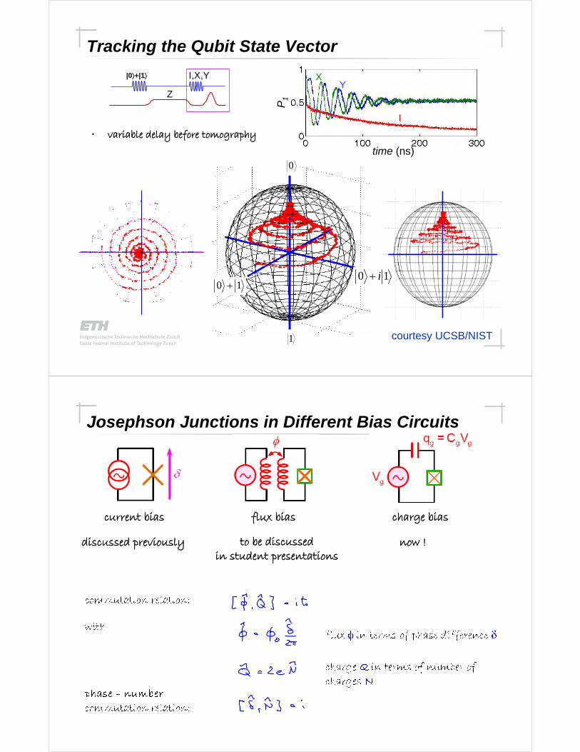
Tracking the Qubit State Vector
courtesy UCSB/NIST
time (ns)
P 1
I,X,Y
I
XY
0
1
10 +10 i+
|0⟩+|1⟩
Z
• variable delay before tomography
Josephson Junctions in Different Bias Circuits
current bias flux bias charge bias
discussed previously to be discussed in student presentations
now !

of Cooper pair box Hamiltonian:
with
Equivalent solution to the Hamiltonian can be found in both representations, e.g. by numerically solving the Schrödinger equation for the charge ( )representation or analytically solving the Schrödinger equation for the phase ( ) representation.
solutions for :
• crossing points arecharge degeneracy points

energy levels for finite EJ=0:
• energy bands are formed
• bands are periodic in Ng
energy bands for finite EJ
• EJ scales level separation at charge degeneracy
Energy Levels
Charge QubitsCooper pair box
electrostatic energy Josephson energy
V. Bouchiat, D. Vion, P. Joyez, D. Esteve, and M. H. Devoret,
Physica Scripta T76, 165 (1998).

Tuning the Josephson Energysplit Cooper pair box in perpendicular field
SQUID modulation of Josephson energy
J. Clarke, Proc. IEEE 77, 1208 (1989)
consider two state approximation
Two-State Approximation
Nakamura, Pashkin, Tsai et al. Nature 398, 421, 425 (1999,2003, 2003)

Control of Charge Qubit
experimental implementation
energy splitting
control parameter
gate charge
effective Hamiltonian
Implementation of Single Qubit Rotations
Z
1
0
X
Y
t
x,y rotations by microwave pulses
1 . 5 2 . 0 2 . 5 3 . 0 3 . 5 4 . 0
- 5 0
0
5 0
1 6 G H zπ p u ls e
Mic
row
ave
outp
ut v
olta
ge
(mV
)
t im e ( n s )
z rotations by adiabatic pulses
full control over quantum state of two level system !
E. Collin et al. Phys. Rev. Lett. 93, 157005 (2004)

Single Qubit Control
Larmor Precession

Coherent Control
coherentoscillations
initial state final state
The First Solid State Qubit - Ever
Y. Nakamura et al., Nature 398, 786 (1999)
φ
SQUID SQUID looploop
ProbeProbeBox Box GateGate
Tunnel Tunnel junctionjunction
SingleSingleCooperCooper--pair pair tunnelingtunneling ReservoirReservoir
• Cooper pair box with probe junction for measurement
• read out by measurement of average current
• first successful experiment

Rabi Oscillations
Y. Nakamura et al., Nature 398, 786 (1999)
P(1)
detuning
Δt
• picosecond fast pulses enable first time-resolved measurement despite short coherence time
• start of superconducting quantum information processing

Superconducting Qubits in Microwave Resonators
• strong qubit - light interactions
• coherent exchange of single quanta (photons) between a qubit and a cavity
Why to put a qubit into a resonator?
• communication between qubits via photons
• non-local qubit/qubit gate interactions
• protection of qubits from spontaneous emission
• quantum non-demolition qubit read-out
benefits for quantum computation:
• quantum optics experiments with circuits
• cavity quantum electrodynamics
• single photon generation and detection
other interesting aspects:
Outline
• What is cavity quantum electrodynamics?
• How to realize it with superconducting circuits
• demonstration of the concept (vacuum Rabi oscillations)
• applications for quantum information processing

Cavity Quantum Electrodynamics (CQED)
D. Walls, G. Milburn, Quantum Optics (Spinger-Verlag, Berlin, 1994)
Dressed States Energy Level Diagram
Atomic cavity quantum electrodynamics reviews:
H. Mabuchi, A. C. Doherty Science 298, 1372 (2002)
J. M. Raimond, M. Brune, & S. Haroche Rev. Mod. Phys. 73, 565 (2001)

Review: J. M. Raimond, M. Brune, and S. Haroche
Rev. Mod. Phys. 73, 565 (2001)
P. Hyafil, ..., J. M. Raimond, and S. Haroche,
Phys. Rev. Lett. 93, 103001 (2004)
Vacuum Rabi Oscillations with Rydberg Atoms
Vacuum Rabi Mode Splitting with Alkali Atoms
R. J. Thompson, G. Rempe, & H. J. Kimble,
Phys. Rev. Lett. 68 1132 (1992)
A. Boca, ... , J. McKeever, & H. J. Kimble
Phys. Rev. Lett. 93, 233603 (2004)

Circuit QED Architecture
A. Blais, R.-S. Huang, A. Wallraff, S. M. Girvin, and R. J. Schoelkopf,PRA 69, 062320 (2004)
elements
• the cavity: a superconducting 1D transmission line resonator (large E0)
• the artificial atom: a Cooper pair box (large d)
Realization
A. Wallraff, D. Schuster, ..., S. Girvin, and R. J. Schoelkopf,
Nature (London) 431, 162 (2004)

Vacuum Field in 1D Cavity
Cavity Properties
• photon lifetime (quality factor) controlled by coupling Cin/out

Resonator Quality Factor and Photon Lifetime
The Artificial Atom: A Cooper Pair Box

The Cooper Pair Box
Resonant Strong Coupling Cavity QED

Bare Resonator Transmission Spectrum
Vacuum Rabi Mode Splitting
A. Wallraff, D. Schuster, ..., S. Girvin, and R. J. Schoelkopf,
Nature (London) 431, 162 (2004)

Coherent Dynamics with Single Photons
Yale Universitycharge qubit & transmission line res.
Nature (London) 431, 162 (2004)
TU Delftflux qubit & SQUID osc.
Nature (London) 431, 159 (2004)
NTTflux qubit & LC res.PRL 96, 127006 (2006)
Strong Coupling Cavity QED
superconductor flux and charge qubitsNature (London) 431, 159 & 162 (Sept. 2004)
alkali atomsRempe, Kimble, ...
Rydberg atomsHaroche, Walther, ...
semiconductor quantum dotsNature (London) 432, 197 & 200 (Nov. 2004)
single trapped atomPRL 93, 233603 (Dec. 2004)

Dispersive (Non-Resonant) Qubit Readout
A. Blais et al., PRA 69, 062320 (2004)
Coherent Control and Read-out in a Cavity

Coherent Control of a Qubit in a Cavity
Time-Resolved Dispersive QND Readout
Wallraff, Schuster, Blais, ... Girvin, and Schoelkopf,
Phys. Rev. Lett. 95, 060501 (2005)

Varying the Control Pulse Length
Wallraff, Schuster, Blais, ... Girvin, and Schoelkopf, Phys. Rev. Lett. 95, 060501 (2005)
High Visibility Rabi Oscillations
A. Wallraff, D. I. Schuster, A. Blais, L. Frunzio, J. Majer,
S. M. Girvin, and R. J. Schoelkopf, Phys. Rev. Lett. 95, 060501 (2005)

High Fidelity Control & Read Out
Long Coherence Time
A. Wallraff et al., Phys. Rev. Lett. 95, 060501 (2005)

Circuit QED and Quantum Optics
Circuit QED and Quantum Computation

2 Qubits
Coupled Qubits

Coupled Qubit Device
Resonator Response
-0.3 -0.2 -0.1 0 0.1 0.2gate voltage, Vg @arb.D
4.6
4.8
5
5.2
xulfsaib,F
@bra.D

Coupling Scheme: Virtual Photon Exchange
A. Blais, R.-S. Huang, A. Wallraff, S. M. Girvin, and R. J. Schoelkopf, PRA 69, 062320 (2004)

row of qubits in a linear Paul trap formsa quantum register
Ion trap quantum processor Laser pulses manipulateindividual ions
A CCD camera reads out the ion`s quantum state
Effective ion-ioninteraction induced bylaser pulses that excitethe ion`s motion
slides courtesy ofHartmut Haeffner, Innsbruck Group

Trapping Individual Ions

Photo-multiplier
CCDcamera
Fluorescencedetection by
CCD cameraphotomultiplier
Vacuumpum
p
oven
atomic
beam
Laser beams for:
photoionizationcoolingquantum state manipulationfluorescence excitation
Experimental setup


Ions with optical transition to metastable level: 40Ca+,88Sr+,172Yb+
P1/2 D5/2
τ =1s
S1/2
40Ca+
P1/2
S1/2
D5/2
Dopplercooling Sideband
cooling
metastable
Ions as Quantum Bits
opticaltransition
stable|g>
|e>
detection
Quadrupole transition
Qubit levels:
P1/2
S1/2
D5/2
S1/2 , D5/2
τ ≈ 1 s
Qubit transition:
S1/2 – D5/2
absorption and emissioncause fluorescence steps(digital quantum jump signal)
D
S
P
S
D
monitorweak transition
metastablelevel
Quantum jumps: spectroscopy with quantized fluorescence
Observation of quantum jumps:
Nagourney et al., PRL 56,2797 (1986),Sauter et al., PRL 57,1696 (1986),
Bergquist et al., PRL 57,1699 (1986)
„ Quantum jump technique“„ Electron shelving technique“
long lifetimeshort lifetime
no photons
lots of photons
time in excited state (average is lifetime)
Detection of Ion Quantum State

Electron shelving for quantum state detection
1. Initialization in a pure quantum state
3. Quantum state measurementby fluorescence detection
2. Quantum state manipulation onS1/2 – D5/2 transition
One ion : Fluorescence histogram
counts per 2 ms0 20 40 60 80 100 120
0
1
2
3
4
5
6
7
8S1/2 stateD5/2 state
P1/2 D5/2
τ =1s
S1/2
40Ca+
P1/2
S1/2
D5/2P1/2
S1/2
D5/2
Quantum statemanipulation
P1/2
S1/2
D5/2
Fluorescencedetection
50 experiments / s
Repeat experiments100-200 times
1. Initialization in a pure quantum state
3. Quantum state measurementby fluorescence detection
2. Quantum state manipulation onS1/2 – D5/2 transition
5µm
50 experiments / s
Repeat experiments100-200 times
Spatially resolveddetection withCCD camera:
Two ions:
P1/2
S1/2
D5/2
Fluorescencedetection
Electron shelving for quantum state detection

Mechanical Quantum harmonical oscillator
Extension of the ground state:
Size of the wave packet << wavelength of visible light
Energy scale of interest:
harmonic trap
ions need to be very cold to be in their vibrationalground state
Mechanical Motion of Ions in their Trapping Potential:
Laser – ion interactions
g
e
⊗
2-level-atom harmonic trap
.. .
0,g
0,e
1,e2,e
2,g
1,g
joint energy levels
…
Approximations:
Electronic structure of the ion approximated by two-level system
(laser is (near-) resonant and couples only two levels)
Trap: Only a single harmonic oscillator taken into account
Ion:
An Ion Coupled to a Harmonic Oscillator
tensor product dressed states diagram

harmonic trap
…
2-level-atom joint energy levels
. . .
External degree of freedom: ion motion
ion transition frequency 400 THz
trap frequency 1 MHz
A closer look at the excitation spectrum (3 ions)
carrier transitionmotional sidebands
Laser detuning Δ at 729 nm (MHz)
motional sidebands
(red / lower) (blue / upper)
many different vibrational modes of ions in the trap

breathing mode cannot be excited on center ion
red and blue side bands can be observed because vibrational motion of ions is not cooled (in this example)
4.54 4.52 4.5 4.48 0
0.2
0.4
0.6
0.8
P D
Detuning δω (MHz) 4.48 4.5 4.52 4.54 0
0.2
0.4
0.6
0.8
P D
Detuning δω (MHz)
99.9 % ground state population
after sideband cooling
after Doppler cooling
7.1=zn
Sideband absorption spectra
red sideband blue sideband
-4.54 -4.52 -4.5 -4.48
Cooling of the vibrational modes
1, −ng
1, −ne
ne,
ng,
……
red side band transition

Coherent excitation on the sideband
...
1, −nS
1, −nD
nD,1, +nD
1, +nS
nS,
coupled system
...
„Blue sideband“ pulses:
D state population
Entanglement between internal and motional state !
But also controlled excitation of the vibrational modes
Single qubit operations
• Laser slightly detuned from carrier resonance
or:
• Concatenation of two pulses with rotation axis in equatorial plane
Arbitrary qubit rotations:
(z-rotations by off-resonant laser beamcreating ac-Stark shifts)
Gate time : 1-10 μs Coherence time : 2-3 ms
limited by
• laser frequency fluctuations
• magnetic field fluctuations
(laser linewidth δν<100 Hz)
D state population
z-rotations
x,y-rotations

CCD
Paul trap
Fluorescencedetection
electro-opticdeflector
coherentmanipulationof qubits
dichroicbeamsplitter
inter ion distance: ~ 4 µm
addressing waist: ~ 2 µm
< 0.1% intensity on neighbouring ions
-10 -8 -6 -4 -2 0 2 4 6 8 100
0.1
0.2
0.3
0.4
0.5
0.6
0.7
0.8
Exc
itatio
n
Deflector Voltage (V)
Addressing the qubits
Generation of Bell states
Pulse sequence:
…
… …
…
generation of entanglement between two ions

Generation of Bell states
Ion 1: π/2 , blue sideband
Pulse sequence:
…
… …
…creates entangled state between qubit 1 and oscillator
Generation of Bell states
Ion 1: π/2 , blue sideband
Ion 2: π , carrier
Pulse sequence:
…
… …
…
excites qubit 2

Generation of Bell states
Ion 1: π/2 , blue sideband
Ion 2: π , carrier
Ion 2: π , blue sideband
Pulse sequence:
…
… …
…
takes qubit 2 (with one oscillator excitation) back to ground state and removes excitation from oscillator
|SD0> is non-resonant and remains unaffected
Bell state analysis
Fluorescencedetection withCCD camera:
Coherent superposition or incoherent mixture ?
What is the relative phase of the superposition ?
SSSD
DSDD SSSDDSDD
Ψ+
Measurement of the density matrix:
tomography of qubit states (= full measurement of x,y,z components of both qubits and its correlations)

A measurement yields the z-component of the Bloch vector
=> Diagonal of the density matrix
Rotation around the x- or the y-axis prior tothe measurement yields the phase informationof the qubit.
(a naïve persons point of view)
=> coherences of the density matrix
Obtaining a single qubits density matrix
as discussed before!
Bell state reconstruction
SSSD
DSDD SSSDDSDD
SSSD
DSDD SSSDDSDD
F=0.91

Phase gate CNOT
Both, the phase gate as well the CNOT gate can be converted into each other with single qubit operations.
Together with the three single qubit gates,we can implement any unitary operation!
phase gate
Quantum gate proposals with trapped ions
Some other gate proposals by:• Cirac & Zoller • Mølmer & Sørensen, Milburn• Jonathan, Plenio & Knight• Geometric phases• Leibfried & Wineland
...allows the realization of a universal quantum computer !

1ε 2ε
Cirac - Zoller two-ion phase gate
ion 1
motion
ion 2
,S D
,S D
0 0SWAP
, 0S,1S
, 0D,1D
1ε 2ε
Cirac - Zoller two-ion phase gate
Phase gate usingthe motion andthe target bit.
ion 1
motion
ion 2
,S D
,S D
0 0SWAP
Z

1ε 2ε
Cirac - Zoller two-ion phase gate
, 0S,1S
, 0D,1D
ion 1
motion
ion 2
,S DSWAP
,S D
0 0SWAP
Z
1ε 2ε
Cirac - Zoller two-ion phase gate
Phase gate usingthe motion andthe target bit.
ion 1
motion
ion 2
,S D
,S D
0 0
Z

Cirac-Zoller phase gate: the key step
0,D1,D
1,S0,S
A 2π pulse is applied to only one of ion-(crystal)s states => only onestates acquires a phase factor of –1.
An additional Zeeman level can be used as the auxilary state.
=> gate is sensitive to magnetic field fluctuations!
How do you do with just a two-level system?
?

Phase gate
Composite 2π-rotation:
A phase gate with 4 pulses (2π rotation)
( ) ( ) ( ) ( )1 1 1 1( , ) , 2 2,0 , 2 2,0R R R R Rθ φ π π π π π π+ + + +=
1
2
3
4
,0 ,1S D↔on2π

A single ion composite phase gate: Experiment
0=ϕ 0=ϕ 2πϕ =2πφ =
0 20 40 60 80 100 120 140 160 1800
0.1
0.2
0.3
0.4
0.5
0.6
0.7
0.8
0.9
1
Time (μs)
D5/
2-
exci
tatio
n2π 2π ππ
2πφ =0=φ 0=φ
state preparation ,0S , then application of phase gate pulse sequence
Testing the phase of the phase gate |0,S>
Time (μs)
D5/
2-
exci
tatio
n
0 50 100 150 200 250 3000
0.1
0.2
0.3
0.4
0.5
0.6
0.7
0.8
0.9
1
Phase gate 2
π−
2
π
97.8 (5) %

ion 1
motion
ion 2
,S DSWAP
,S D
0 0
control qubit
target qubit
SWAP
ion 1
ion 2
pulse sequence:
Cirac - Zoller two-ion controlled-NOT operation
Cirac – Zoller CNOT gate operation
SS - SS DS - DD
SD - SD DD - DS

input
output
Measured truth table of Cirac-Zoller CNOT operation
Superposition as input to CNOT gate
outputprepare gate detect

Two qubit gate
Decoherence issues
Implementation of an algorithm
Scaling of ion trap quantum computers
Quantum computing with trapped ions (part 2)
Contents
row of qubits in a linear Paul trap formsa quantum register
Ion trap quantum processor Laser pulses manipulateindividual ions
A CCD camera reads out the ion`s quantum state
Effective ion-ioninteraction induced bylaser pulses that excitethe ion`s motion

Experimental setup
Ca+
S1/2
P1/2D5/2
qubit(qutrit,or more)
0,S
0,D1,D
1,S
carrier
sideband
D-s
tate
pop
ulat
ion
Coherent manipulation

0,S
0,D1,D
1,S
carrier and blue sidebandRabi oscillations
with Rabi frequencies
carrier
sideband
is the Lamb-Dicke parameter
and
Coherent manipulation
Quantum gate proposals with trapped ions
Some other gate proposals by:• Cirac & Zoller • Mølmer & Sørensen, Milburn• Jonathan, Plenio & Knight• Geometric phases• Leibfried & Wineland
...allows the realization of a universal quantum computer !

1ε 2ε
Cirac - Zoller two-ion phase gate
ion 1
motion
ion 2
,S D
,S D
0 0SWAP
, 0S,1S
, 0D,1D
1ε 2ε
Cirac - Zoller two-ion phase gate
Phase gate usingthe motion andthe target bit.
ion 1
motion
ion 2
,S D
,S D
0 0SWAP
Z

1ε 2ε
Cirac - Zoller two-ion phase gate
, 0S,1S
, 0D,1D
ion 1
motion
ion 2
,S DSWAP
,S D
0 0SWAP
Z
1ε 2ε
Cirac - Zoller two-ion phase gate
Phase gate usingthe motion andthe target bit.
ion 1
motion
ion 2
,S D
,S D
0 0
Z

The key step: phase gate
?
0 10 20 30 40 50 60 700
0.1
0.2
0.3
0.4
0.5
0.6
0.7
0.8
0.9
1
Time (μs)
D-s
tate
pop
ulat
ion
Phase switched by π/2
The other type of Rabi oscillations

+
What is this phase ?
+
-
The electric field of the laser drives a dipole transition …
+
What is this phase ?
-
+
The electric field of the laser drives a dipole transition …

Phase gate
Composite 2π-rotation:
A phase gate with 4 pulses
( ) ( ) ( ) ( )1 1 1 1( , ) , 2 2,0 , 2 2,0R R R R Rθ φ π π π π π π+ + + +=
1
2
3
4
,0 ,1S D↔on2π

A single ion composite phase gate: Experiment
0=ϕ 0=ϕ 2πϕ =2πφ =
0 20 40 60 80 100 120 140 160 1800
0.1
0.2
0.3
0.4
0.5
0.6
0.7
0.8
0.9
1
Time (μs)
D5/
2-e
xcita
tion
2π 2π ππ2πφ =0=φ 0=φ
state preparation ,0S , then application of phase gate pulse sequence
Population of |S,1> - |D,2> remains unaffected
( ) ( ) ( ) ( )1 1 1 1( , ) 2, 2 ,0 2, 2 ,0R R R R Rθ φ π π π π π π+ + + +=
4
3
2
1

Testing the phase of the phase gate |0,S>
Time (μs)
D5/
2-e
xcita
tion
0 50 100 150 200 250 3000
0.1
0.2
0.3
0.4
0.5
0.6
0.7
0.8
0.9
1Phase gate 2
π−
2
π
97.8 (5) %
Phase gate with starting in |D,1>
0 50 100 150 200 250 3000
0.1
0.2
0.3
0.4
0.5
0.6
0.7
0.8
0.9
1
D5/
2-e
xcita
tion
Time (μs)
Phase gate 2π
−2
πBlueπ

ion 1
motion
ion 2
,S DSWAP
,S D
0 0
control qubit
target qubit
SWAP
ion 1
ion 2
pulse sequence:
Cirac - Zoller two-ion controlled-NOT operation
Control bitControl bit Target bitTarget bit
Truth table of the CNOT
outputinput
Probability

Superposition as input to CNOT gate
outputprepare gate detect
Two qubit gate
Decoherence issues
Implementation of an algorithm
Scaling of ion trap quantum computers

Error budget for Cirac-Zoller CNOT
3 %5 % in Rabi frequency(at neighbouring ion)
Addressing error(can be corrected for partially)
~ 1 %~ 3 Hz (FWHM)Laser frequency noise
(Phase coherence)
Fidelity lossMagnitudeError source
9 %
~ 3 %
0.3 %
< 1 %0.4 %
November 2006Total
~ 500 Hz (FWHM)Laser detuning error
5 % peak to peakLaser intensity noise
<n>bus < 0.01<n>spec = 6
Residual thermal excitation
Testing the phase of the phase gate |0,S>
Time (μs)
D5/
2-e
xcita
tion
0 50 100 150 200 250 3000
0.1
0.2
0.3
0.4
0.5
0.6
0.7
0.8
0.9
1Phase gate 2
π−
2
π
97.8 (5) %

Time
Ramsey experiment
Quantum algorithms can be viewed as generalized Ramsey experiments!
Laser detuning (kHz)
Phase coherence
⇒ Gaussian modell yields a coherence time of 0.9 ms 2005: 2 ms are more typical.2007: 8 ms are more typical.

( )
( )
( )
( )DSSD
DDSS
DSSD
DDSS
−=Ψ
−=Φ
+=Ψ
+=Φ
−
−
+
+
2
12
12
12
1CNOT
DD
SD
DS
SS Ion 1
Ion 2
Creating entangled states with a CNOT
SSSD
DSDD SSSDDSDD
SSSD
DSDD SSSDDSDD
SSSD
DSDD SSSDDSDD
long lived (~ 1000 ms) short lived (1 ms)
Ene
rgy
see e.g. Kielpinski et al.,Science 291, 1013-1015 (2001)
SSSD
DSDD SSSDDSDD
Ene
rgy
Lifet
ime
limite
d on
ly by
spon
tant
eous
dec
ay o
f the
D le
vel
Lifet
ime
limite
d on
ly by
spon
tant
eous
dec
ay o
f the
D le
vel
Lifet
ime
limite
d by
lase
r fre
quen
cy st
abilit
y
Lifet
ime
limite
d by
lase
r fre
quen
cy st
abilit
y
Decoherence of entangled states

Two qubit gate
Decoherence issues
Implementation of an algorithm
Scaling of ion trap quantum computers
Alice
Bob
Bell state
unknowninput state
Teleportation
recoverinput state
rotation
classical communication
measurementin Bell basis
Bennett et al., Phys. Rev. Lett. 70, 1895 (1993)

Alice: Measurement in Bell state basis
unknown state EPR pair
Blue=AliceRed=Bob
Principle of Teleportation
Ion 3
Ion 2
Ion 1
Bell
state
initialize #1, #2, #3
classicalcommunication
conditionalrotations
CNOT --Bell basis
Alice
Bob
Selectiveread out
Implementation of the teleportation protocol
recoveredon ion #3

Teleportation: Rotate into the Bell basisTeleportation: Rotate into the Bell basis
Bell
state
( )
( )
( )
( )DSSD
DDSS
DSSD
DDSS
−=Ψ
−=Φ
+=Ψ
+=Φ
−
−
+
+
2
12
12
12
1CNOT
DD
SD
DS
SS Ion 1
Ion 2
Creating entangled states with a CNOT

( )
( )
( )
( )DSSD
DDSS
DSSD
DDSS
−=Ψ
−=Φ
+=Ψ
+=Φ
−
−
+
+
2
12
12
12
1 CNOT
DD
SD
DS
SSIon 1
Ion 2
And now backwards ...
Superposition as input to a CNOT gate
prepare CNOT detect

And now backwards ...
Teleportation: Selective read-out of a quantum registerTeleportation: Selective read-out of a quantum register
Bell
state

Selective read-out of the ion string
We want to read out some ions without disturbing thecoherence of the neighbouring ions.This is required for
- most error correction protocols.- teleportation.- having fun with the ions.
1. The ions are spaced by about 5 μm.2. One photon projects an ion onto the measurement basis.
Where is the problem?
Selective read out
D5/2
S1/2S1/2
ion #1
D5/2
S1/2S1/2
ion #2
D5/2
S1/2S1/2
ion #3
qutrits

D5/2
S1/2S1/2
ion #1
D5/2
S1/2S1/2
ion #2
D5/2
S1/2S1/2
ion #3
photonscattering
ion 1 ismeasured
protected !
detect quantum state of ion #1 only
Selective read out
Ion 3
Ion 2
Ion 1
−1Ψ
conditional rotationsusing electronic logic, triggered by PM signal
conditional rotationsusing electronic logic, triggered by PM signalP
U
U
P
C C C
Ψ
B
B B B B C
CU P
B
C
C P
spin echo sequencespin echo sequence
full sequence:26 pulses + 2 measurements
full sequence:26 pulses + 2 measurements
B
C
blue sidebandpulsesblue sidebandpulses
carrier pulsescarrier pulses
P
C
B
B
Teleportation protocol, details

Input test states Output statesInitial Final
TPU U-1
Ion #1 Ion #3
Teleportation procedure, analysis

Fidelity: 0.83
Classicalthreshold
Quantum teleportation on demand
Teleportation on demand, however, only 10 μm.
Process tomography of teleportation

What is teleportation good for?
Supose you can somehow entangle two qubits in different quantum computers with some dirty trick.
1. Teleport the first qubit to the second one.2. Do a gate operation involving the second one.
Effectively you have now performed a quantum gatebetween two distant places where at this time now quantum channel was available
See Gottesman and Chuang, Nature 402 390-393 (1999), for details.
qubit
qubit(quoctet)
Encoding of quantum information requires long-lived atomic states:
microwave transitions
9Be+, 25Mg+, 43Ca+, 87Sr+, 137Ba+, 111Cd+, 171Yb+
optical transitions
Ca+, Sr+, Ba+, Ra+, Yb+, Hg+ etc.
S1/2
P1/2D5/2
S1/2
P3/2
Qubits with trapped ions

Raman transitions: motional sidebands
effective Lamb Dicke parameter
copropagating Raman beams for excitation of carrier transitions
(no sideband transitions)
counterpropagating Raman beams for efficient excitation of sideband transitions
orbeams from different directions
P3/2
P1/2
S1/2
|n=0⟩
|n=3⟩ |n=0⟩
|n=3⟩
F↓= - F↑
Entangling interactions: controlled phase gate
Use Raman beams that couple the motional states (but not internal states)
F↓
Raman beams form (moving) standing wave: spatial light shifts
x
ΔE
F↑
State dependent optical dipole force

Stretch mode excitation
no differential force
no differential force
differential force
differential force
Boulder group :Gate fidelity: 97%Gate time: 7 μs (ca. 25/νCOM)
D. Leibfried et al., Nature 422, 414 (2003)Theory: Milburn, Fortschr. Phys. 48, 9(2000)
Sørensen&Mølmer
Phase space picture

Realized time scales in ion trap systems
10-6 s
10-1 s
103 s
10-4 s
10-3 s
101 s
Single qubit gates
Two qubit gates (Geometric phase gate, Boulder)
Single qubit coherence (magnetic field sensitive)
Coherence of the motion (Innsbruck)
Decoherence free subspaces
Well chosen single qubit coherence (Boulder)
10-5 s
10-2 s
100 s
102 s
Two qubit gates (Cirac-Zoller approach)
Single qubit coherence (magnetic field insensitive, Boulder)
Two qubit gate
Decoherence issues
Implementation of an algorithm
Scaling of ion trap quantum computers

Easy to have thousands of ions in a trap and to manipulate them individually…
but it is hard to control their interaction!
Scaling ion trap quantum computers
Scaling of the Cirac-Zoller approach?
• Coupling strength between internal and motional states of a N-ion stringdecreases as
(momentum transfer from photon to ion stringbecomes more difficult)
-> Gate operation speed slows down
• More vibrational modes increase risk of spurious excitation of unwanted modes
-> Use flexible trap potentials to split long ion string into smaller segmentsand perform operations on these smaller strings
Problems :
• Distance between neighbouring ions decreases -> addressing more difficult

Easy to have thousands of ions in a trap and to manipulate them individually…
but it is hard to control their interaction!
Scaling ion trap quantum computers
Kielpinski, Monroe, Wineland
The solution:The solutions:
Cirac, Zoller, Kimble, Mabuchi Tian, Blatt, Zoller
“accumulator”
controlqubit
targetqubit
D. Wineland, Boulder, USAKieplinski et al, Nature 417, 709 (2002)
Idea #1: move the ions around

Segmented ion traps as scalable trap architecture
(ideas pioneered by D. Wineland, NIST, and C. Monroe, Univ. Michigan)
Segmented trap electrode allow totransport ions and to split ion strings
Transport of ions
1 mm within 50 μs
no motional heating
Splitting of two-ion crystal
tseparation ≈ 200 μssmall heating Δn ≈1
State of the art:
„Architecture for a large-scale ion-trap quantum computer“, D. Kielpinski et al, Nature 417, 709 (2002)
„Transport of quantum states“, M. Rowe et al, quant-ph/0205084
D. Wineland (NIST) : Alumina / gold trap

Coherent transport of quantum information
C. Monroe (Michigan) : GaAs-GaAlAs trap

1
NMR Quantum Computing
Slides courtesy of Lieven Vandersypen (now at TU Delft)with some annotations by Andreas Wallraff.
2
How to factor 15 with NMR?
Lieven Vandersypen
Then: IBM Almaden, Stanford University
Now: Kavli Institute of NanoScience, TU Delft
F
F13C12C
F
12CF
F
13C
C5H5 CO
Fe
1
3
54
26
7
CO red nuclei are qubits: F, 13C
perfluorobutadienyliron complex

3
Goals of this tutorial
Survey of NMR quantum computing
Perspective on building a quantum computer
How would you factor 15?
Principles of NMR QCTechniques for qubit controlExample: factoring 15State of the artOutlook
4
NMR largely satisfies the DiVincenzo criteria
Qubits: nuclear spins ½ in B0 field ( ↑ and ↓ as 0 and 1)
Quantum gates: RF pulses and delay times
( ) Input: Boltzman distribution (room temperature)
Readout: detect spin states with RF coil
Coherence times: easily several seconds
(Gershenfeld & Chuang 1997, Cory, Havel & Fahmi 1997)
13CCl
ClCl
1H

5
Nuclear spin HamiltonianSingle spin
6
Nuclear spin HamiltonianMultiple spins
(at 11.7 Tesla)
1H13C15N19F31P
500
126
-51
470
202
MHz
without qubit/qubitcoupling
qubit level separation
chemical shiftsof the five F qubits
~ 25 mK

7
Hamiltonian with RF fieldsingle-qubit rotations
Rotating frame Lab frame
typical strength Ix, Iy : up to 100 kHz
σz σx σy
rotating wave approximation
8
Nuclear spin HamiltonianCoupled spins
Typical values: J up to few 100 Hz
coupling term
solid (dashed) lines are (un)coupled levels
J>0: antiferro mag.
J<0: ferro-mag.
16 configurations

9
Controlled-NOT in NMR
if spin B is ↑
YA90 XA
90Delay1/2JAB
if spin B is ↓
Before After
A B A B
↑ ↑ ↑ ↑↑ ↓ ↓ ↓↓ ↑ ↓ ↑↓ ↓ ↑ ↓
” flip A if B ↓”
xy
z
xy
z
xy
z
xy
z
xy
z
xy
z
xy
z
xy
z
| 0 ⟩
| 1 ⟩
| 0 ⟩ + i | 1 ⟩√2
| 0 ⟩ + | 1 ⟩√2
time
A target bitB control bit
wait
different rotation direction depending on control bit
10
Making room temperature spins look cold↑↑ ↑↓ ↓↑ ↓↓
(Cool to mK)
Optical pumping
DNP, …
↑↑
↑↓ ↓↑ ↓↓
Effective pure state(Gershenfeld&Chuang, Science ‘97, Cory, Havel & Fahmi, PNAS ‘97)
↑↑↑↓ ↓↑ ↓↓
Look exactly like cold spins !
[Hz] [Hz]
low
ener
gy
high
ener
gy
cold
warm
quasi cold
warmquasi cold
equalize population

11
Effective pure state preparation
(1) Add up 2N-1 experiments (Knill,Chuang,Laflamme, PRA 1998)
Later ≈ (2N - 1) / N experiments (Vandersypen et al., PRL 2000)
(2) Work in subspace (Gershenfeld&Chuang, Science 1997)
↑↑ ↑↓ ↓↑ ↓↓ ↑↑ ↑↓ ↓↑ ↓↓ ↑↑ ↑↓ ↓↑ ↓↓ ↑↑ ↑↓ ↓↑ ↓↓
+ + =
↑↑↑ ↑↑↓ ↑↓↑ ↑↓↓ ↓↑↑ ↓↑↓ ↓↓↑ ↓↓↓ ↑↑↑ ↑↑↓ ↑↓↑ ↑↓↓ ↓↑↑ ↓↑↓ ↓↓↑ ↓↓↓
compute with qubit states that have the same energy and thus the same population.
prepare equal population (on average) and look at deviations fromequilibrium.
12
Read-out in NMR |0⟩ |0⟩
|0⟩ |1⟩
|1⟩ |0⟩
|1⟩ |1⟩
Phase sensitive detection
Y90
xy
z
x
y
z
Y90
xy
z
xy
z
|1⟩
|0⟩
negative signal for |1> (out of phase)
positive signal for |0> (in phase)

13
Measurements of single systems versus ensemble measurements
|00⟩
|0⟩ and |0⟩bitwise average
“word”wise average
single-shot bitwise
single-shot “word”wise
|0⟩ and |0⟩
|00⟩
|00⟩
quantum state |00⟩ + |11⟩
|00⟩ or |11⟩
each bit average of |0⟩ and |1⟩
each bit |0⟩ or |1⟩
average of |00⟩ and |11⟩
QC
NMR
adapt algorithms if use ensemble
14
Quantum state tomography
xy
z
xy
z
xy
z
xy
z
after X90
xy
z
xy
z
Look at qubits from different angles
after Y90
xy
z
xy
z
xy
z
no pulse

16
Outline
Survey of NMR quantum computing
Principles of NMR QCTechniques for qubit controlExample: factoring 15State of the artOutlook
17
Off-resonance pulses and spin-selectivity
spectral content of a square pulse
may induce transitions in other qubits
off-resonant pulses induce eff. σz rotation in addition to σx,y

18
Pulse shaping for improved spin-selectivity
gaussian pulse profile gaussian spectrum
less cross-talk
19
Missing coupling terms: Swap
Missing couplings: swap states along qubit network
SWAP12 = CNOT12 CNOT21 CNOT12
“only” a linear overhead ...
1 2 3 4
How to couple distant qubits with only nearest neighbor physical couplings?
as discussed in exercise class

20
Undesired couplings: refocus
• There exist efficient extensions for arbitrary coupling networks• Refocusing can also be used to remove unwanted Zeeman terms
XB180 XB
180
XA180XA
180
remove effect of coupling during delay timesopt. 1: act on qubit B
opt. 2: act on qubit A
22
Composite pulses
Example: Y90X180Y90
corrects for under/over-rotation
corrects for off-resonance
However: doesn’t work for arbitrary input stateBut: there exist composite pulses that work for all input states
x y
z
x y
z

24
Molecule selection
spins 1/2 (1H, 13C, 19F, 15N, ...)
long T1’s and T2’s
heteronuclear, or large chemical shifts
good J-coupling network (clock-speed)
stable, available, soluble, ...
A quantum computer is a known molecule.
Its desired properties are:
required to make spins of same type addressable
25
Quantum computer molecules (1)
Grover / Deutsch-Jozsa
CCl
Cl
Cl
H
C CF
BrF
F
C CH
Cl
Cl
Cl
H
N
OC
O
C
H H3
CH3
TeleportationLogical labeling / Grover
Q. Error correction
CHO
O-Na+
Q. Error Detection
red nuclei are used as qubits:

26
Quantum computer molecules (2)
Deutsch-Jozsa 7-spin coherence
Order-finding
O
N
O
CD
CH F
D
O
CC
CC
H
H
H3O
OH
C CC
F
CFF
F
F
Fe(CH)5 (CO)2
27
Outline
Survey of NMR quantum computing
Principles of NMR QCTechniques for qubit controlExample: factoring 15State of the artOutlook

28
Quantum Factoring
f (x) = a x mod N
composite number
coprime with N
Results from number theory:
f is periodic in x (period r)
gcd(a r/2 ± 1, N ) is a factor of N
Quantum: ~ L 3 P. Shor (1994)Complexity of factoring numbers of length L: Classically: ~ e L/3
Widely used crypto systems (RSA) would become insecure.
Quantum factoring: find r
Find the prime factors of N: chose a and find order r.
29
Factoring 15 - schematic
H
x a x mod N
QFT
|x⟩ = |0⟩ + |1⟩ + ... + |22L-1⟩
|x⟩
L=log2(15)
2 L bits
4 qubitsΣ |x⟩ | a x mod 15 ⟩x
|0⟩
|1⟩
Σ |k2L/r⟩k
Interference
a = 2, 7, 8, 13 ⇒ a4 mod 15 = 1 ⇒ “hard” casea = 4, 11 ⇒ a2 mod 15 = 1 ⇒ “easy” case
a = 14 ⇒ fails
3 qubitsQuantum parallelism
x = ... + x2 22 + x1 21 + x0 20
ax = ... a4 a2 ax2 x1 x0 ...
...
x a 2x a 1 x a 4
x0x1x2

30
Quantum Fourier transform and the FFT
[ 1 1 1 1 1 1 1 1 ]
[ 1 . 1 . 1 . 1 . ]
[ 1 . . . 1 . . . ]
[ 1 . . . . . . . ]
[ 1 . . . 1 . . . ]
[ . 1 . . . 1 . . ]
[ . . 1 . . . 1 . ]
[ . . . 1 . . . 1 ]
[ 1 . . . . . . . ]
[ 1 . . . 1 . . . ]
[ 1 . 1 . 1 . 1 . ]
[ 1 1 1 1 1 1 1 1 ]
[ 1 . 1 . 1 . 1 . ]
[ 1 . -i . -1 . i . ]
[ 1 . -1 . 1 . -1 . ]
[ 1 . i . -1 . -i . ]
FFT
The FFT (and QFT)
Inverts the period
Removes the off-set
|ψ3⟩ = |0⟩ |0⟩ + |1⟩ |2⟩ + |2⟩ |0⟩ + |3⟩ |2⟩ + |4⟩ |0⟩ + |5⟩ |2⟩ + |6⟩ |0⟩ + |7⟩ |2⟩= ( |0⟩ + |2⟩ + |4⟩ + |6⟩ ) |0⟩ + ( |1⟩ + |3⟩ + |5⟩ + |7⟩ ) |2⟩
|ψ4⟩ = ( |0⟩ + |4⟩ ) |0⟩ + ( |0⟩ - |4⟩ ) |2⟩
hard
easy
31
12 34
5
Experimental approach11.7 Tesla Oxford superconducting magnet; room temperature bore
4-channel Varian spectrometer; need to address and keep track of 7 spins
phase ramped pulses
software reference frame
Shaped pulses
Compensate for cross-talk
Unwind coupling during pulses
F
F13C12C
F
12CF
F13C
C5H5 (CO)2
Fe
Larmor frequencies
470 MHz for 19F
125 MHz for 13C
J - couplings: 2 - 220 Hz
coherence times: 1.3 - 2 s
469.98 470.00 470.02 [MHz]1
3
54
2
6
7~25 mK

32
Picture of the lab
33
Thermal Equilibrium Spectra
• line splitting due to J-coupling• all lines present
1 2 34 5
Rea
l par
t [ar
b. u
nits
]R
eal p
art [
arb.
uni
ts]
Rea
l par
t [ar
b. u
nits
]
[Hz]
[Hz]
Qubit 1
Qubit 2
[Hz]
Qubit 3uncoupled qubit states indicated by arrows

34
Spectra after state initialization
RT spins appear cold!
Rea
l par
t [ar
b. u
nits
]
[Hz]
[Hz] [Hz]
Rea
l par
t [ar
b. u
nits
]
Rea
l par
t [ar
b. u
nits
]
• only the |00 … 0 ⟩ line remains• the other lines are averaged away
by adding up multiple experiments
Qubit 1
Qubit 2 Qubit 3
35
Pulse sequence (a=7)
> 300 pulses, ≈ 720 ms
π/2 X- or Y-rotations (H and gates)π X-rotations (refocusing)Z - rotations

36
|000⟩ 0Qubit 1:up |0⟩
Qubit 2:up |0⟩
Qubit 3:up/down |0⟩,|1⟩
“Easy” case (a=11)
8 / r = 4r = 2
15 = 3 x 5
gcd(112/2 - 1, 15) = 5
gcd(112/2 + 1, 15) = 3Rea
l par
t [ar
b. u
nits
]R
eal p
art [
arb.
uni
ts]
Imag
par
t [ar
b. u
nits
]
321
|100⟩ 4
Ideal prediction
Experiment
[Hz]
[Hz] [Hz]
recall read-out scheme
period
37
“Hard” case (a=7)
8 / r = 2r = 4
15 ≅ 3 x 5
gcd(74/2 - 1, 15) = 3
gcd(74/2 + 1, 15) = 5Rea
l par
t [ar
b. u
nits
]Im
ag p
art [
arb.
uni
ts]
Imag
par
t [ar
b. u
nits
]
|000⟩ 0|010⟩ 2|100⟩ 4|110⟩ 6Qubit 1:
up |0⟩
Qubit 3:up/down |0⟩,|1⟩
Qubit 2:up/down |0⟩,|1⟩
[Hz]
[Hz] [Hz]
period
decoherence

38
Model quantum noise (decoherence)
phaserandomization
energyexchange
Spins interact with the environment
Decoherence
We created a workable decoherence model for 7 coupled spins.The model is parameter free.
The decoherence model for 1 nuclear spin is well-described.
39
fundamental limit
Simulation of decoherence (1)
Rea
l par
t [ar
b. u
nits
]Im
ag p
art [
arb.
uni
ts]
Imag
par
t [ar
b. u
nits
]
hard case
[Hz]
[Hz] [Hz]
decoherence can be understood and modeled

40
Simulation of decoherence (2)
fundamental limit
Rea
l par
t [ar
b. u
nits
]R
eal p
art [
arb.
uni
ts]
Imag
par
t [ar
b. u
nits
]
easy case
[Hz]
[Hz] [Hz]
decoherence can be understood and modeled
41
Outline
Survey of NMR quantum computing
Principles of NMR QCTechniques for qubit controlExample: factoring 15State of the artOutlook

42# qubits
1 2 3 4 5 6 7
# ga
tes
and
gate
net
wor
k
State of the art in various qubit systems
NMR
F
F13C12C
F
12CF
F
13C
C5H5 CO
Fe
1
3
54
26
7
CO
0.2 mmtrapped
ions
Courtesy D. Wineland, NIST
Trapped ionsSuperconducting
Courtesy Y. Nakamura, NEC
Excitons, atoms
e -
43
The good news
Quantum computations have been demonstrated in the lab
A high degree of control was reached, permitting hundreds of
operations in sequence
A variety of tools were developed for accurate unitary control
over multiple coupled qubits
useful in other quantum computer realizations
Spins are natural, attractive qubits

44
Scaling
We do not know how to scale liquid NMR QC
Main obstacles:
• Signal after initialization ~ 1 / 2n [at least in practice]
• Coherence time typically goes down with molecule size
• We have not yet reached the accuracy threshold ...
45
Main sources of errors in NMR QC
Early on (heteronuclear molecules)
inhomogeneity RF field
Later (homonuclear molecules)
J coupling during RF pulses
Finally
decoherence

46
Solid-state NMR ?
Yamaguchi & Yamamoto, 2000
molecules insolid matrix
Cory et al
47
Electron spin qubits
SL SR
Loss & DiVincenzo, PRA 1998Kane, Nature 1998

48
Factoring 15 Vandersypen et al., Nature 414, 883 (2001)
Qubit control Vandersypen & Chuang, RMP, to appear Oct 2004
Intro Gershenfeld and Chuang, Scientific American, June 1998Survey Cory, et al., Fortschr. Phys. 48, 875, 2000.Survey Jones, Fortschr. Phys., 48, 909, 2000.Survey Cory, Chuang et al., recent preprint (arXiv.org/???)
References

Quantum Information Processing with Semiconductor Quantum Dots
slides courtesy of Lieven Vandersypen, TU Delft

A seven-spin NMR quantum computer
F
F13C12C
F
12CF
F
13C
C5H5 CO
Fe
13
54
26
7
CO
Vandersypen et al., Nature 414, 883 (2001)Vandersypen & Chuang, RMP, Oct 2004.
15 = 3 x 5

Kane, Nature 1998
SL SR
Loss & DiVincenzoPRA 1998
Imamoglu et al, PRL 1999
at the level of single-particles?
in a solid state environment?
Can we access the quantum world

Electrically controlled and measured quantum dots
A small semiconducting (or metallic) island where electrons are confined, giving a discrete level spectrum
Vsd Vg
GATE
ISLANDDRAINSOURCE
I
e
Vsd Vg
GATE
ISLANDDRAINSOURCE
IVsd Vg
GATE
ISLANDDRAINSOURCE
Vsd Vg
GATE
ISLANDDRAINSOURCE
I
e
• Coupled via tunnel barriers to source and drain reservoirs• Coupled capacitively to gate electrode, to control # of electrons

Examples of quantum dots
single molecule self-assembled QD
nanotube
1 nm 10 nm 1µm
lateral QD
100 nm
metallic nanoparticle vertical QD nanowire

Electrostatically defined quantum dots
• Electrically measured (contact to 2DEG)• Electrically controlled number of electrons• Electrically controlled tunnel barriers

Dilution refrigerator
300 K
1 K
4 K
10 mK
~ 10 cm~ 1m

Spin qubits in quantum dots SL SRLoss & DiVincenzo, PRA 1998Vandersypen et al., Proc. MQC02 (quant-ph/0207059)
Initialization 1-electron, low T, high B0
H0 ~ Σ ωi σzi
Read-out convert spin to charge
then measure charge↑ ↓
Coherence long relaxation time T1long coherence time T2
ESR pulsed microwave magnetic fieldHRF ~ Σ Ai(t) cos(ωi t) σxi
↑
↓EZ = gµBB
↑
↓EZ = gµBB
SWAP exchange interaction HJ ~ Σ Jij (t) σi · σj
↑ ↓J(t)↑ ↓J(t)

Transport through quantum dot -Coulomb blockade
-1350 -1400 -1450 -1500 -1550 -1600 -1650
Gate Voltage [mV]
0
10
20
30
40
50
Cur
rent
dot
[pA
]
µL µR
Is this the last electron ??
µN=1
µN=2
µN=3

A quantum point contact (QPC)as a charge detector Field et al, PRL 1993
-0.80 -0.85 -0.90 -0.95 -1.000
2
Con
duct
ance
(e2 /h
)
QPC gate voltage (V)-1.17 -1.20 -1.23 -1.26 -1.29
1.0
1.5
2.0
QP
C C
urre
nt (n
A)
Dot plunger voltage (V)

The last electron!
N=2 N=1 N=0
-1350 -1400 -1450 -1500 -1550 -1600 -16500
500
1000
1500
2000
Cur
rent
QPC
[pA
]
Gate Voltage [mV]
0
10
20
30
40
50
Dot
cur
rent
[pA
]
Sprinzak et al ’01

Few-electron double dot designCiorga et al ’99
Open design
Field et al’93Sprinzak et al ’01
QPC for charge detection
200 nm
T
ML RPL PR
QPC-R
IDOT
IQPCIQPC
QPC-L
NTT (T. Saku, Y. Hirayama)Sumitomo ElectricUniversität Regensburg (W. Wegscheider)
GaAs/AlGaAs wafers:
Elzerman et al., PRB 2003

Few-electron double dotMeasured via QPC
-0.96
-1.02
-0.15 -0.30
00
10
01
11
2221
12
V L(V
)
VPR(V)
-0.9
-1.1
0 -0.6
00
V L(V
)
VPR(V)
• Double dot can be emptied• QPC can detect all charge transitions
dIQPC/dVL
J.M. Elzerman et al., PRB 67, R161308 (2003)
0 Tesla

Single electron tunneling throughtwo dots in series
ΓL ΓR
ΓL ΓR
µS
Vg
µDµS
Vg1
ΓR
Vg
µD
Vg2
µDµ(N,N+1)
µ(N+1,N)
ΓL

Few-electron double dotTransport through dots
J. Elzerman et al., cond-mat/0212489
-0.96
-1.02
-0.15 -0.30
00
10
01
11
2221
12
V L(V
)
VPR(V)
Peak height
< 1 pA
2 pA
70 pA

Energy level spectroscopy at B = 0
B = 0 T
10
-10
0
-653 -695
V SD
N=1
VT (mV)
dIDOT/dVSD
• ∆E ~ 1.1meV
• EC ~ 2.5meV
N=0
(mV
)
Ground and excited state
transport
Ground state
transport
DRAINSOURCE
Γ
200 nm M P R
Q
T
Notransport

Single electron Zeeman splitting in B//
Hanson et al, PRL 91, 196802 (2003)Also: Potok et al, PRL 91, 016802 (2003)
0 T
2
-2
0 N=0
V SD
(mV
)
GSES
↑
↓B=0 B> 0
gµBB
-995 -1010VR (mV)10 T
N=0
-675VT (mV)
N=1
2
-2
0
-657
6 T
V SD
(mV
)
N=0N=1
0 5 10 150
0.1
0.2
B// (T)
∆E Z
(meV
)
|g|=0.44

Initialization of a single electron spin
Method 1:spin-selectivetunneling
Method 2:relaxation toground state

Spin qubits in quantum dots SL SRLoss & DiVincenzo, PRA 1998Vandersypen et al., Proc. MQC02 (quant-ph/0207059)
Initialization 1-electron, low T, high B0
H0 ~ Σ ωi σzi
Read-out convert spin to charge
then measure charge↑ ↓
Coherence long relaxation time T1long coherence time T2
ESR pulsed microwave magnetic fieldHRF ~ Σ Ai(t) cos(ωi t) σxi
↑
↓EZ = gµBB
↑
↓EZ = gµBB
SWAP exchange interaction HJ ~ Σ Jij (t) σi · σj
↑ ↓J(t)↑ ↓J(t)