LECTURE NOTES ON THE PRINCIPAL AGENT MODEL · PRINCIPAL AGENT MODEL 1. SIMPLIFIED MODEL 2....

LECTURE NOTES ON THE

PRINCIPAL AGENT MODEL

1

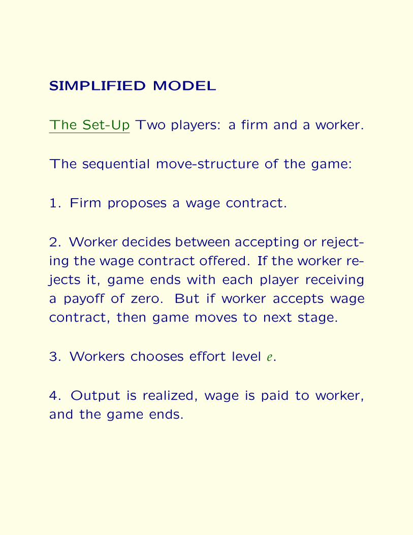
SIMPLIFIED MODEL

2

SIMPLIFIED MODEL

The Set-Up Two players: a firm and a worker.

SIMPLIFIED MODEL


The sequential move-structure of the game:

1. Firm proposes a wage contract.

SIMPLIFIED MODEL




2. Worker decides between accepting or reject-

ing the wage contract offered. If the worker re-

jects it, game ends with each player receiving

a payoff of zero. But if worker accepts wage

contract, then game moves to next stage.

SIMPLIFIED MODEL









3. Workers chooses effort level e.

SIMPLIFIED MODEL









3. Workers chooses effort level e.

4. Output is realized, wage is paid to worker,

and the game ends.

Given effort, e: with probability ηe, output is

high and revenue associated with that is v. But

with probability 1 − ηe, no output is produced

and zero revenue obtained. The former is a

case of the ”project” on which worker works

being a success, while the latter a failure.

So note that worker’s effort generates ”ran-

dom” output.

3








dom” output.

All players are risk neutral.








dom” output.


Expected profit to firm is: Eπ = (ηe)v − w,

where w is wage.








dom” output.


Expected profit to firm is: Eπ = (ηe)v − w,

where w is wage.

Expect Utility to worker is: EU = w− ce2

3 , where

c > 0.

FIRST-BEST EFFORT LEVEL

4


Maximize Eπ such that EU ≥ u.



That is, choose e to maximize social surplus:




maxe

ηev − ce2

3.




maxe

ηev − ce2

3.

First-Order condition:

ηv =2ce3

.




maxe

ηev − ce2

3.

First-Order condition:

ηv =2ce3

.

Hence, first-best effort level is:

e∗ =3ηv2c

.

FIRM CANNOT OBSERVE EFFORT, BUT

ONLY OUTPUT LEVEL.

5


ONLY OUTPUT LEVEL.

Hence, firm’s wage contract cannot be condi-

tioned on e.


ONLY OUTPUT LEVEL.


tioned on e.

But instead, firm’s wage contract is condi-

tioned on observable and verifiable output.


ONLY OUTPUT LEVEL.


tioned on e.

But instead, firm’s wage contract is condi-

tioned on observable and verifiable output.

So, wage contract is a pair: (wS, wF), where

wS is wage when output is high (ie., project is

a success) and wF is wage when output is low

(zero – project is a failure).

Worker’s problem:

maxe

EU = (ηe)wS + (1 − ηe)wF − ce2

3.

6

Worker’s problem:

maxe


3.

FOC:

η(wS − wF) =2ce3

.

Worker’s problem:

maxe


3.

FOC:

η(wS − wF) =2ce3

.

This implies that the subgame perfect equilib-

rium (SPE) effort level is:

e =3η(wS − wF)

2c. (1)

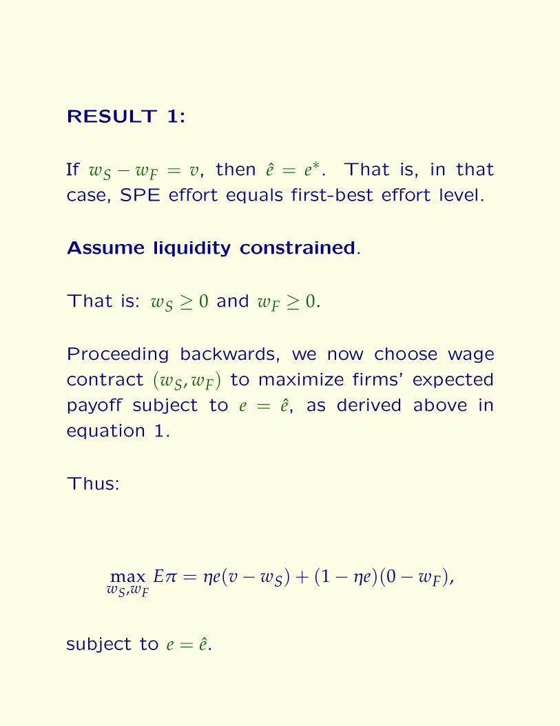
RESULT 1:

If wS − wF = v, then e = e∗. That is, in that

case, SPE effort equals first-best effort level.

7

RESULT 1:



Assume liquidity constrained.

That is: wS ≥ 0 and wF ≥ 0.

RESULT 1:





Proceeding backwards, we now choose wage

contract (wS, wF) to maximize firms’ expected

payoff subject to e = e, as derived above in

equation 1.

RESULT 1:





Proceeding backwards, we now choose wage

contract (wS, wF) to maximize firms’ expected

payoff subject to e = e, as derived above in

equation 1.

Thus:

maxwS,wF

Eπ = ηe(v − wS) + (1 − ηe)(0 − wF),

subject to e = e.

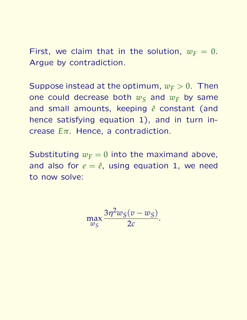
First, we claim that in the solution, wF = 0.

Argue by contradiction.

8



Suppose instead at the optimum, wF > 0. Then

one could decrease both wS and wF by same

and small amounts, keeping e constant (and

hence satisfying equation 1), and in turn in-

crease Eπ. Hence, a contradiction.



Suppose instead at the optimum, wF > 0. Then

one could decrease both wS and wF by same

and small amounts, keeping e constant (and

hence satisfying equation 1), and in turn in-

crease Eπ. Hence, a contradiction.

Substituting wF = 0 into the maximand above,

and also for e = e, using equation 1, we need

to now solve:

maxwS

3η2wS(v − wS)

2c.

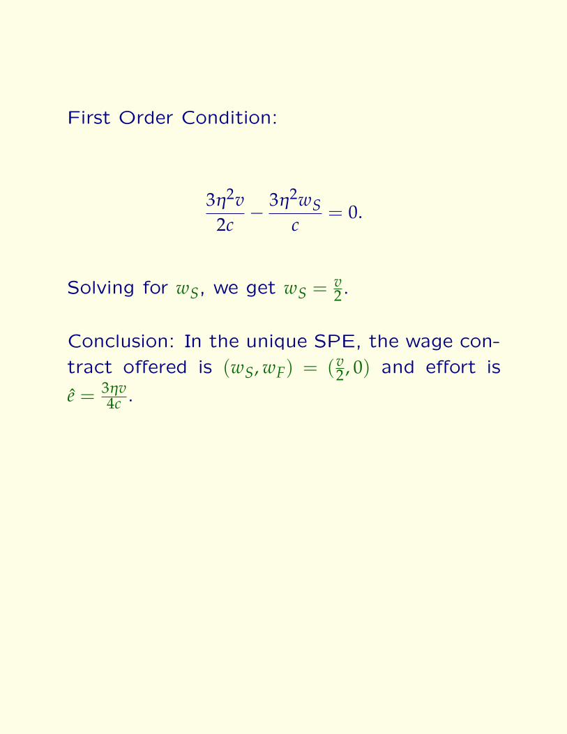
First Order Condition:

3η2v2c

− 3η2wSc

= 0.

9


3η2v2c

− 3η2wSc

= 0.

Solving for wS, we get wS = v2.

Conclusion: In the unique SPE, the wage con-

tract offered is (wS, wF) = (v2 , 0) and effort is

e = 3ηv4c .


3η2v2c

− 3η2wSc

= 0.

Solving for wS, we get wS = v2.

Conclusion: In the unique SPE, the wage con-

tract offered is (wS, wF) = (v2 , 0) and effort is

e = 3ηv4c .

NOTE, the SPE effort is less than first-best

effort.

LECTURE NOTES ON THE PRINCIPAL AGENT MODEL · PRINCIPAL AGENT MODEL 1. SIMPLIFIED MODEL 2....

Documents

Transcript of LECTURE NOTES ON THE PRINCIPAL AGENT MODEL · PRINCIPAL AGENT MODEL 1. SIMPLIFIED MODEL 2....