LECTURE NOTES ON PROBABILITY, STATISTICS AND LINEAR...

LECTURE NOTES ON PROBABILITY,STATISTICS AND LINEAR ALGEBRA

C. H. TaubesDepartment of Mathematics

Harvard UniversityCambridge, MA 02138

Spring, 2010

CONTENTS

1 Data Exploration 21.1 Snowfall data . . . . . . . . . . . . . . . . . . . . . . . . . . . . . . . . . . . . . . . . . . . . . . . 31.2 Data mining . . . . . . . . . . . . . . . . . . . . . . . . . . . . . . . . . . . . . . . . . . . . . . . 31.3 Exercises . . . . . . . . . . . . . . . . . . . . . . . . . . . . . . . . . . . . . . . . . . . . . . . . . 6

2 Basic notions from probability theory 72.1 Talking the talk . . . . . . . . . . . . . . . . . . . . . . . . . . . . . . . . . . . . . . . . . . . . . . 72.2 Axiomatic definition of probability . . . . . . . . . . . . . . . . . . . . . . . . . . . . . . . . . . . 92.3 Computing probabilities for subsets . . . . . . . . . . . . . . . . . . . . . . . . . . . . . . . . . . . 112.4 Some consequences of the definition . . . . . . . . . . . . . . . . . . . . . . . . . . . . . . . . . . 122.5 That’s all there is to probability . . . . . . . . . . . . . . . . . . . . . . . . . . . . . . . . . . . . . 132.6 Exercises . . . . . . . . . . . . . . . . . . . . . . . . . . . . . . . . . . . . . . . . . . . . . . . . . 13

3 Conditional probability 163.1 The definition of conditional probability . . . . . . . . . . . . . . . . . . . . . . . . . . . . . . . . . 163.2 Independent events . . . . . . . . . . . . . . . . . . . . . . . . . . . . . . . . . . . . . . . . . . . . 173.3 Bayes theorem . . . . . . . . . . . . . . . . . . . . . . . . . . . . . . . . . . . . . . . . . . . . . . 183.4 Decomposing a subset to compute probabilities . . . . . . . . . . . . . . . . . . . . . . . . . . . . . 193.5 More linear algebra . . . . . . . . . . . . . . . . . . . . . . . . . . . . . . . . . . . . . . . . . . . . 223.6 An iterated form of Bayes’ theorem . . . . . . . . . . . . . . . . . . . . . . . . . . . . . . . . . . . 223.7 Exercises . . . . . . . . . . . . . . . . . . . . . . . . . . . . . . . . . . . . . . . . . . . . . . . . . 23

4 Linear transformations 254.1 Protein molecules . . . . . . . . . . . . . . . . . . . . . . . . . . . . . . . . . . . . . . . . . . . . 254.2 Protein folding . . . . . . . . . . . . . . . . . . . . . . . . . . . . . . . . . . . . . . . . . . . . . . 26

5 How matrix products arise 275.1 Genomics . . . . . . . . . . . . . . . . . . . . . . . . . . . . . . . . . . . . . . . . . . . . . . . . . 275.2 How bacteria find food . . . . . . . . . . . . . . . . . . . . . . . . . . . . . . . . . . . . . . . . . . 285.3 Growth of nerves in a developing embryo . . . . . . . . . . . . . . . . . . . . . . . . . . . . . . . . 295.4 Enzyme dynamics . . . . . . . . . . . . . . . . . . . . . . . . . . . . . . . . . . . . . . . . . . . . 295.5 Exercises . . . . . . . . . . . . . . . . . . . . . . . . . . . . . . . . . . . . . . . . . . . . . . . . . 29

6 Random variables 316.1 The definition of a random variable . . . . . . . . . . . . . . . . . . . . . . . . . . . . . . . . . . . 316.2 Probability for a random variable . . . . . . . . . . . . . . . . . . . . . . . . . . . . . . . . . . . . 326.3 A probability function on the possible values of f . . . . . . . . . . . . . . . . . . . . . . . . . . . 336.4 Mean and standard distribution for a random variable . . . . . . . . . . . . . . . . . . . . . . . . . . 336.5 Random variables as proxies . . . . . . . . . . . . . . . . . . . . . . . . . . . . . . . . . . . . . . . 346.6 A biology example . . . . . . . . . . . . . . . . . . . . . . . . . . . . . . . . . . . . . . . . . . . . 36

i

6.7 Independent random variables and correlation matrices . . . . . . . . . . . . . . . . . . . . . . . . . 376.8 Correlations and proteomics . . . . . . . . . . . . . . . . . . . . . . . . . . . . . . . . . . . . . . . 396.9 Exercises . . . . . . . . . . . . . . . . . . . . . . . . . . . . . . . . . . . . . . . . . . . . . . . . . 39

7 The statistical inverse problem 417.1 A general setting . . . . . . . . . . . . . . . . . . . . . . . . . . . . . . . . . . . . . . . . . . . . . 447.2 The Bayesian guess . . . . . . . . . . . . . . . . . . . . . . . . . . . . . . . . . . . . . . . . . . . 447.3 An example . . . . . . . . . . . . . . . . . . . . . . . . . . . . . . . . . . . . . . . . . . . . . . . . 457.4 Gregor Mendel’s peas . . . . . . . . . . . . . . . . . . . . . . . . . . . . . . . . . . . . . . . . . . 457.5 Another candidate for P(θ): A maximum likelihood candidate. . . . . . . . . . . . . . . . . . . . . 467.6 What to remember from this chapter . . . . . . . . . . . . . . . . . . . . . . . . . . . . . . . . . . . 487.7 Exercises . . . . . . . . . . . . . . . . . . . . . . . . . . . . . . . . . . . . . . . . . . . . . . . . . 49

8 Kernel and image in biology 50

9 Dimensions and coordinates in a scientific context 529.1 Coordinates . . . . . . . . . . . . . . . . . . . . . . . . . . . . . . . . . . . . . . . . . . . . . . . . 529.2 A systematic approach . . . . . . . . . . . . . . . . . . . . . . . . . . . . . . . . . . . . . . . . . . 539.3 Dimensions . . . . . . . . . . . . . . . . . . . . . . . . . . . . . . . . . . . . . . . . . . . . . . . . 539.4 Exercises . . . . . . . . . . . . . . . . . . . . . . . . . . . . . . . . . . . . . . . . . . . . . . . . . 54

10 More about Bayesian statistics 5510.1 A problem for Bayesians . . . . . . . . . . . . . . . . . . . . . . . . . . . . . . . . . . . . . . . . . 5510.2 A second problem . . . . . . . . . . . . . . . . . . . . . . . . . . . . . . . . . . . . . . . . . . . . 5510.3 Meet the typical Bayesian . . . . . . . . . . . . . . . . . . . . . . . . . . . . . . . . . . . . . . . . 5510.4 A first example . . . . . . . . . . . . . . . . . . . . . . . . . . . . . . . . . . . . . . . . . . . . . . 5610.5 A second example . . . . . . . . . . . . . . . . . . . . . . . . . . . . . . . . . . . . . . . . . . . . 5710.6 Something traumatic . . . . . . . . . . . . . . . . . . . . . . . . . . . . . . . . . . . . . . . . . . . 5710.7 Rolling dice . . . . . . . . . . . . . . . . . . . . . . . . . . . . . . . . . . . . . . . . . . . . . . . 5810.8 Exercises . . . . . . . . . . . . . . . . . . . . . . . . . . . . . . . . . . . . . . . . . . . . . . . . . 58

11 Common probability functions 5911.1 What does ‘random’ really mean? . . . . . . . . . . . . . . . . . . . . . . . . . . . . . . . . . . . . 5911.2 A mathematical translation of the term ‘random’ . . . . . . . . . . . . . . . . . . . . . . . . . . . . 5911.3 Some standard counting solutions . . . . . . . . . . . . . . . . . . . . . . . . . . . . . . . . . . . . 6011.4 Some standard probability functions . . . . . . . . . . . . . . . . . . . . . . . . . . . . . . . . . . . 6111.5 Means and standard deviations . . . . . . . . . . . . . . . . . . . . . . . . . . . . . . . . . . . . . . 6411.6 The Chebychev theorem . . . . . . . . . . . . . . . . . . . . . . . . . . . . . . . . . . . . . . . . . 6511.7 Characteristic functions . . . . . . . . . . . . . . . . . . . . . . . . . . . . . . . . . . . . . . . . . 6611.8 Loose ends about counting elements in various sets . . . . . . . . . . . . . . . . . . . . . . . . . . . 6711.9 A Nobel Prize for the clever use of statistics . . . . . . . . . . . . . . . . . . . . . . . . . . . . . . . 6811.10 Exercises . . . . . . . . . . . . . . . . . . . . . . . . . . . . . . . . . . . . . . . . . . . . . . . . . 70

12 P-values 7212.1 Point statistics . . . . . . . . . . . . . . . . . . . . . . . . . . . . . . . . . . . . . . . . . . . . . . 7212.2 P -value and bad choices . . . . . . . . . . . . . . . . . . . . . . . . . . . . . . . . . . . . . . . . . 7312.3 A binomial example using DNA . . . . . . . . . . . . . . . . . . . . . . . . . . . . . . . . . . . . . 7412.4 An example using the Poisson function . . . . . . . . . . . . . . . . . . . . . . . . . . . . . . . . . 7512.5 Another Poisson example . . . . . . . . . . . . . . . . . . . . . . . . . . . . . . . . . . . . . . . . 7612.6 A silly example . . . . . . . . . . . . . . . . . . . . . . . . . . . . . . . . . . . . . . . . . . . . . . 7712.7 Exercises . . . . . . . . . . . . . . . . . . . . . . . . . . . . . . . . . . . . . . . . . . . . . . . . . 78

13 Continuous probability functions 8013.1 An example . . . . . . . . . . . . . . . . . . . . . . . . . . . . . . . . . . . . . . . . . . . . . . . . 8013.2 Continuous probability functions . . . . . . . . . . . . . . . . . . . . . . . . . . . . . . . . . . . . 80

ii

13.3 The mean and standard deviation . . . . . . . . . . . . . . . . . . . . . . . . . . . . . . . . . . . . 8113.4 The Chebychev theorem . . . . . . . . . . . . . . . . . . . . . . . . . . . . . . . . . . . . . . . . . 8113.5 Examples of probability functions . . . . . . . . . . . . . . . . . . . . . . . . . . . . . . . . . . . . 8213.6 The Central Limit Theorem: Version 1 . . . . . . . . . . . . . . . . . . . . . . . . . . . . . . . . . 8313.7 The Central Limit Theorem: Version 2 . . . . . . . . . . . . . . . . . . . . . . . . . . . . . . . . . 8413.8 The three most important things to remember . . . . . . . . . . . . . . . . . . . . . . . . . . . . . . 8513.9 A digression with some comments on Equation (13.1) . . . . . . . . . . . . . . . . . . . . . . . . . 8513.10 Exercises . . . . . . . . . . . . . . . . . . . . . . . . . . . . . . . . . . . . . . . . . . . . . . . . . 86

14 Hypothesis testing 8814.1 An example . . . . . . . . . . . . . . . . . . . . . . . . . . . . . . . . . . . . . . . . . . . . . . . . 8814.2 Testing the mean . . . . . . . . . . . . . . . . . . . . . . . . . . . . . . . . . . . . . . . . . . . . . 8914.3 Random variables . . . . . . . . . . . . . . . . . . . . . . . . . . . . . . . . . . . . . . . . . . . . 9014.4 The Chebychev and Central Limit Theorems for random variables . . . . . . . . . . . . . . . . . . . 9014.5 Testing the variance . . . . . . . . . . . . . . . . . . . . . . . . . . . . . . . . . . . . . . . . . . . 9114.6 Did Gregor Mendel massage his data? . . . . . . . . . . . . . . . . . . . . . . . . . . . . . . . . . . 9214.7 Boston weather 2008 . . . . . . . . . . . . . . . . . . . . . . . . . . . . . . . . . . . . . . . . . . . 9414.8 Exercises . . . . . . . . . . . . . . . . . . . . . . . . . . . . . . . . . . . . . . . . . . . . . . . . . 95

15 Determinants 97

16 Eigenvalues in biology 9916.1 An example from genetics . . . . . . . . . . . . . . . . . . . . . . . . . . . . . . . . . . . . . . . . 9916.2 Transition/Markov matrices . . . . . . . . . . . . . . . . . . . . . . . . . . . . . . . . . . . . . . . 10016.3 Another protein folding example . . . . . . . . . . . . . . . . . . . . . . . . . . . . . . . . . . . . . 10016.4 Exercises . . . . . . . . . . . . . . . . . . . . . . . . . . . . . . . . . . . . . . . . . . . . . . . . . 102

17 More about Markov matrices 10417.1 Solving the equation . . . . . . . . . . . . . . . . . . . . . . . . . . . . . . . . . . . . . . . . . . . 10517.2 Proving things about Markov matrices . . . . . . . . . . . . . . . . . . . . . . . . . . . . . . . . . . 10617.3 Exercises . . . . . . . . . . . . . . . . . . . . . . . . . . . . . . . . . . . . . . . . . . . . . . . . . 109

18 Markov matrices and complex eigenvalues 11118.1 Complex eigenvalues . . . . . . . . . . . . . . . . . . . . . . . . . . . . . . . . . . . . . . . . . . . 11118.2 The size of the complex eigenvalues . . . . . . . . . . . . . . . . . . . . . . . . . . . . . . . . . . . 11218.3 Another Markov chain example . . . . . . . . . . . . . . . . . . . . . . . . . . . . . . . . . . . . . 11318.4 The behavior of a Markov chain as t→∞ . . . . . . . . . . . . . . . . . . . . . . . . . . . . . . . 11418.5 Exercises . . . . . . . . . . . . . . . . . . . . . . . . . . . . . . . . . . . . . . . . . . . . . . . . . 114

19 Symmetric matrices and data sets 11619.1 An example from biology . . . . . . . . . . . . . . . . . . . . . . . . . . . . . . . . . . . . . . . . 11619.2 A fundamental concern . . . . . . . . . . . . . . . . . . . . . . . . . . . . . . . . . . . . . . . . . . 11619.3 A method . . . . . . . . . . . . . . . . . . . . . . . . . . . . . . . . . . . . . . . . . . . . . . . . . 11719.4 Some loose ends . . . . . . . . . . . . . . . . . . . . . . . . . . . . . . . . . . . . . . . . . . . . . 11819.5 Some examples . . . . . . . . . . . . . . . . . . . . . . . . . . . . . . . . . . . . . . . . . . . . . . 11819.6 Small versus reasonably sized eigenvalues . . . . . . . . . . . . . . . . . . . . . . . . . . . . . . . 11919.7 Exercises . . . . . . . . . . . . . . . . . . . . . . . . . . . . . . . . . . . . . . . . . . . . . . . . . 120

iii

Preface

This is a very slight revision of the notes used for Math 19b in the Spring 2009 semester. These are written by CliffTaubes (who developed the course), but re-formatted and slightly revised for Spring 2010. Any errors you might findwere almost certainly introduced by these revisions and thus are not the fault of the original author.

I would be interested in hearing of any errors you do find, as well as suggestions for improvement of either the text orthe presentation.

Peter M. [email protected]

1

[email protected]

CHAPTER

ONE

Data Exploration

The subjects of Statistics and Probability concern the mathematical tools that are designed to deal with uncertainty. Tobe more precise, these subjects are used in the following contexts:

• To understand the limitations that arise from measurement inaccuracies.

• To find trends and patterns in noisy data.

• To test hypothesis and models with data.

• To estimate confidence levels for future predictions from data.

What follows are some examples of scientific questions where the preceding issues are central and so statistics andprobability play a starring role.

• An extremely large meteor crashed into the earth at the time of the disappearance of the dinosaurs. The mostpopular theory posits that the dinosaurs were killed by the ensuing environmental catastrophe. Does the fossilrecord confirm that the disappearance of the dinosaurs was suitably instantaneous?

• We read in the papers that fat in the diet is “bad” for you. Do dietary studies of large populations support thisassertion?

• Do studies of gene frequencies support the assertion that all extent people are 100% African descent?

• The human genome project claims to have determined the DNA sequences along the human chromosomes. Howaccurate are the published sequences? How much variation should be expected between any two individuals?

Statistics and probability also play explicit roles in our understanding and modelling of diverse processes in the lifesciences. These are typically processes where the outcome is influenced by many factors, each with small effect, butwith significant total impact. Here are some examples:

Examples from Chemistry: What is thermal equilibrium? Does it mean stasis?

Why are chemical reaction rates influenced by temperature? How do proteins fold correctly? How stable are the foldedconfigurations?

Examples from medicine: How many cases of flu should the health service expect to see this winter? How to determinecancer probabilities? Is hormone replacement therapy safe? Are anti-depressants safe?

An example from genomics: How are genes found in long stretches of DNA? How much DNA is dispensable?

An example from developmental biology: How does programmed cell death work; what cells die and what live?

Examples from genetics: What are the fundemental inheritance rules? How can genetics determine ancestral relation-ships?

2

An examples from ecology: How are species abundance estimates determined from small samples?

To summarize: There are at least two uses for statistics and probability in the life sciences. One is to tease informationfrom noisy data, and the other is to develop predictive models in situations where chance plays a pivotal role. Note thatthese two uses of statistics are not unrelated since a theoretical understanding of the causes for the noise can facilitateits removal.

The rest of this first chapter focuses on the first of these two uses of statistics.

1.1 Snowfall data

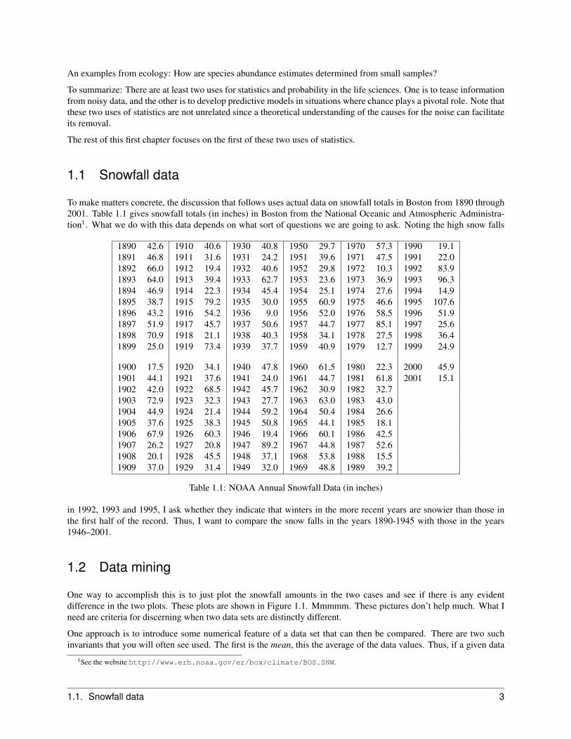
To make matters concrete, the discussion that follows uses actual data on snowfall totals in Boston from 1890 through2001. Table 1.1 gives snowfall totals (in inches) in Boston from the National Oceanic and Atmospheric Administra-tion1. What we do with this data depends on what sort of questions we are going to ask. Noting the high snow falls

1890 42.6 1910 40.6 1930 40.8 1950 29.7 1970 57.3 1990 19.11891 46.8 1911 31.6 1931 24.2 1951 39.6 1971 47.5 1991 22.01892 66.0 1912 19.4 1932 40.6 1952 29.8 1972 10.3 1992 83.91893 64.0 1913 39.4 1933 62.7 1953 23.6 1973 36.9 1993 96.31894 46.9 1914 22.3 1934 45.4 1954 25.1 1974 27.6 1994 14.91895 38.7 1915 79.2 1935 30.0 1955 60.9 1975 46.6 1995 107.61896 43.2 1916 54.2 1936 9.0 1956 52.0 1976 58.5 1996 51.91897 51.9 1917 45.7 1937 50.6 1957 44.7 1977 85.1 1997 25.61898 70.9 1918 21.1 1938 40.3 1958 34.1 1978 27.5 1998 36.41899 25.0 1919 73.4 1939 37.7 1959 40.9 1979 12.7 1999 24.9

1900 17.5 1920 34.1 1940 47.8 1960 61.5 1980 22.3 2000 45.91901 44.1 1921 37.6 1941 24.0 1961 44.7 1981 61.8 2001 15.11902 42.0 1922 68.5 1942 45.7 1962 30.9 1982 32.71903 72.9 1923 32.3 1943 27.7 1963 63.0 1983 43.01904 44.9 1924 21.4 1944 59.2 1964 50.4 1984 26.61905 37.6 1925 38.3 1945 50.8 1965 44.1 1985 18.11906 67.9 1926 60.3 1946 19.4 1966 60.1 1986 42.51907 26.2 1927 20.8 1947 89.2 1967 44.8 1987 52.61908 20.1 1928 45.5 1948 37.1 1968 53.8 1988 15.51909 37.0 1929 31.4 1949 32.0 1969 48.8 1989 39.2

Table 1.1: NOAA Annual Snowfall Data (in inches)

in 1992, 1993 and 1995, I ask whether they indicate that winters in the more recent years are snowier than those inthe first half of the record. Thus, I want to compare the snow falls in the years 1890-1945 with those in the years1946–2001.

1.2 Data mining

One way to accomplish this is to just plot the snowfall amounts in the two cases and see if there is any evidentdifference in the two plots. These plots are shown in Figure 1.1. Mmmmm. These pictures don’t help much. What Ineed are criteria for discerning when two data sets are distinctly different.

One approach is to introduce some numerical feature of a data set that can then be compared. There are two suchinvariants that you will often see used. The first is the mean, this the average of the data values. Thus, if a given data

1See the website http://www.erh.noaa.gov/er/box/climate/BOS.SNW.

1.1. Snowfall data 3

http://www.erh.noaa.gov/er/box/climate/BOS.SNW

1895 1905 1915 1925 1935 19450

20

40

60

80

100

120

Year

Snow

fall

(inc

hes)

................................................................................................................................................................................................................................................................................................................................................................................................................................................................

................................................................................................................................................................................................................................................................................................................................................................................................................................................................

................................................................................................................................................................................................................................................................................................................................................................................................................................................................

................................................................................................................................................................................................................................................................................................................................................................................................................................................................

................................................................................................................................................................................................................................................................................................................................................................................................................................................................

................................................................................................................................................................................................................................................................................................................................................................................................................................................................

••

••

••••

•

••

••

•

••

•

••

•••

•

•

•

•

••

•

•

••

•

••

•

•

•

•

••

•

•

•

•

•

•

••••

•

•

•

••

1950 1960 1970 1980 1990 20000

20

40

60

80

100

120

Year

Snow

fall

(inc

hes)

........................................................................................................................................................................................................................................................................................................................................................................................................................................................................

........................................................................................................................................................................................................................................................................................................................................................................................................................................................................

........................................................................................................................................................................................................................................................................................................................................................................................................................................................................

........................................................................................................................................................................................................................................................................................................................................................................................................................................................................

........................................................................................................................................................................................................................................................................................................................................................................................................................................................................

........................................................................................................................................................................................................................................................................................................................................................................................................................................................................

•

•

•••••••

•••••

•

•

•

•

••

•

•••••

•

••

•

•

•

•

••

•

••

••

••

•

•

••

•

•

•

•

•

•••

•

•

Figure 1.1: Snowfall Data for Years 1890–1945 (left) and 1946–2001 (right)

set consists of an ordered list of of some N numbers, {x1, . . . , xN}, the mean is

µ =1N

(x1 + x2 + · · ·+ xN ) (1.1)

In the cases at hand,µ1890-1945 = 42.4 and µ1946-2001 = 42.3. (1.2)

These are pretty close! But, of course, I don’t know how close two means must be for me to say that there is nostatistical difference between the data sets. Indeed, two data sets can well have the same mean and look very different.For example, consider that the three element sets {−1, 0, 1} and {−10, 0, 10}. Both have mean zero, but the spread ofthe values in one is very much greater than the spread of the values in the other.

The preceding example illustrates the fact that means are not necessarily good criteria to distinguish data sets. Lookingat this last toy example, I see that these two data sets are distinguished in some sense by the spread in the data; byhow far the points differ from the mean value. The standard deviation is a convenient measure of this difference. It isdefined to be

σ =

√1

N − 1((x1 − µ)2 + (x2 − µ)2 + · · ·+ (xN − µ)2

). (1.3)

The standard deviations for the two snowfall data sets are

σ1890-1945 = 16.1 and σ1946-2001 = 21.4. (1.4)

Well, these differ by roughly 5 inches, but is this difference large enough to be significant? How much differenceshould I tolerate so as to maintain that the snowfall amounts are “statistically” identical? How much difference instandard deviations signals a significant difference in yearly snowfall?

I can also “bin” the data. For example, I can count how many years have total snow fall less than 10 inches, then howmany 10–20 inches, how many 20-30 inches, etc. I can do this with the two halves of the data set and then comparebin heights. Here is the result:

1890–1945: 1 2 11 11 16 5 6 4 0 0 01946–2001: 0 8 11 9 11 7 5 0 3 1 1

(1.5)

Having binned the data, I am yet at a loss to decide if the difference in bin heights really signifies a distinct differencein snow fall between the two halves of the data set.

4 Chapter 1. Data Exploration

What follows is one more try at a comparison of the two halves; it is called the rank-sum test and it works as follows: Igive each year a number, between 1 and 112, by ranking the years in order of increasing total snow-fall. For example,the year with rank 1 is 1936 and the years with rank 109 and 110 are 1993 and 1995. I now sum all of the ranks forthe years 1890-1945 to get the rank-sum for the first half of the data set. I then do the same for the years 1946-2001to get the rank-sum for the latter half. I can now compare these two numbers. If one is significantly larger than theother, the data set half with the larger rank-sum has comparatively more high snowfall years than that with the smallerrank-sum. This understood, here are the two rank-sums:

rank-sum1890-1945 = 3137 and rank-sum1946-2001 = 3121. (1.6)

Thus, the two rank-sums differ by 16. But, I am again faced with the following question: Is this difference significant?How big must the difference be to conclude that the first half of the 20’th century had, inspite of 1995, more snow onaverage, than the second half?

To elaborate now on this last question, consider that there is a hypothesis on the table:

The rank-sums for the two halves of the data set indicate that there is a significant difference between thesnowfall totals from the first half of the data set as compared with those from the second.

To use the numbers in (1.6) to analyze the validity of this hypothesis, I need an alternate hypothesis for comparison.The comparison hypothesis plays the role here of the control group in an experiment. This “control” is called the nullhypothesis in statistics. In this case, the null-hypothesis asserts that the rankings are random. Thus, the null-hypothesisis:

The 112 ranks are distributed amongst the years as if they were handed out by a blindfolded monkeychoosing numbers from a mixed bin.

Said differently, the null-hypothesis asserts that the rank-sums in (1.6) are statistically indistinguishable from thosethat I would obtain I were to randomly select 56 numbers from the set {1, 2, 3, . . . , 112} to use for the rankings of theyears in the first half of the data set, while using the remaining numbers for the second half.

An awful lot is hidden here in the phrase statistically indistinguishable. Here is what this phrase means in the caseat hand: I should compute the probability that the sum of 56 randomly selected numbers from the set {1, 2, . . . , 112}differs from the sum of the 56 numbers that are left by at least 16. If this probability is very small, then I have someindication that the snow fall totals for the years in the two halves of the data set differ in a significant way. If theprobability is high that the rank-sums for the randomly selected rankings differ by 16 or more, then the differenceindicated in (1.6) should not be viewed as indicative of some statistical difference between the snowfall totals for theyears in the two halves of the data set.

Thus, the basic questions are:

• What is the probability in the case of the null-hypothesis that I should get a difference that is bigger than theone that I actually got?

• What probability should be considered “significant”?

Of course, I can ask these same two questions for the bin data in (1.5). I can also ask analogs of these question for thetwo means in (1.2) and for the two standard deviations in (1.4). However, because the bin data, as well as the meansand standard deviations deal with the snowfall amounts rather than with integer rankings, I would need a different sortof definition to use for the null-hypothesis in the latter cases.

In any event, take note that the first question is a mathematical one and the second is more of a value choice. The firstquestion leads us to study the theory of probability which is the topic in the next chapter. As for the second question, Ican tell you that it is the custom these days to take 1

20 = 0.05 as the cut-off between what is significant and what isn’t.Thus,

1.2. Data mining 5

If the probability of seeing a larger difference in values than the one seen is less than 0.05, then theobserved difference is deemed to be “significant”.

This choice of 5 percent is rather arbitrary, but such is the custom.

1.3 Exercises:

1. This exercise requires ten minutes of your time on two successive mornings. It also requires a clock that tellstime to the nearest second.

(a) On the first morning, before eating or drinking, record the following data: Try to estimate the passage ofprecisely 60 seconds of time with your eyes closed. Thus, obtain the time from the clock, immediatelyclose your eyes and when you feel that 1 minute has expired, open them and immediately read the amountof time that has passed on the clock. Record this as your first estimate for 1 minute of time. Repeat thisprocedure ten time to obtain ten successive estimates for 1 minute.

(b) On the second morning, repeat this part (a), but first drink a caffeinated beverage such as coffee, tea, or acola drink.

(c) With parts (a) and (b) completed, you have two lists of ten numbers. Compute the means and standarddeviations for each of these data sets. Then, combine the data sets as two halves of a single list of 20numbers and compute the rank-sums for the two lists. Thus, your rankings will run from 1 to 20. In theevent of a tie between two estimates, give both the same ranking and don’t use the subsequent ranking.For example, if there is a tie for fifth, use 5 for both but give the next highest estimate 7 instead of 6.

2. Flip a coin 200 times. Use n1 to denote the number of heads that appeared in flips 1-10, use n2 to denotethe number that appeared in flips 11-20, and so on. In this way, you generate twenty numbers, {n1, . . . n20}.Compute the mean and standard deviation for the sets {n1, . . . n10}, {n11, . . . n20}, and {n1, . . . n20}.

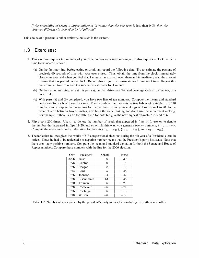
3. The table that follows gives the results of US congressional elections during the 6th year of a President’s term inoffice. (Note: he had to be reelected.) A negative number means that the President’s party lost seats. Note thatthere aren’t any positive numbers. Compute the mean and standard deviation for both the Senate and House ofRepresentatives. Compare these numbers with the line for the 2006 election.

Year President Senate House2006 Bush −6 −301998 Clinton 0 −51986 Reagan −8 −51974 Ford −5 −481966 Johnson −4 −471958 Eisenhower −13 −481950 Truman −6 −291938 Roosevelt −6 −711926 Coolidge −6 −101918 Wilson −6 −19

Table 1.2: Number of seats gained by the president’s party in the election during his sixth year in office

6 Chapter 1. Data Exploration

CHAPTER

TWO

Basic notions from probability theory

Probability theory is the mathematics of chance and luck. To elaborate, its goal is to make sense of the followingquestion:

What is the probability of a given outcome from some set of possible outcomes?

For example, in the snow fall analysis of the previous chapter, I computed the rank-sums for the two halves of thedata set and found that they differed by 16. I then wondered what the probability was for such rank sums to differ bymore than 16 if the rankings were randomly selected instead of given by the data. We shall eventually learn what itmeans to be “randomly selected” and how to compute such probabilities. However, this comes somewhat farther intothe course.

2.1 Talking the talk

Unfortunately for the rest of us, probability theory has its own somewhat arcane language. What follows is a list ofthe most significant terms. Treat this aspect of the course as you would any other language course. In any event, thereare not so many terms, and you will soon find that you don’t have to look back at your notes to remember what theymean.

Sample space: A sample space is the set of all possible outcomes of the particular “experiment” of interest. Forexample, in the rank-sum analysis of the snowfall data from the previous chapter, I should consider the sample spaceto be the set of all collections of 56 distinct integers from the collection {1, . . . , 112}.

For a second example, imagine flipping a coin three times and recording the possible outcomes of the three flips. Inthis case, the sample space is

S = {TTT, TTH, THT,HTT, THH,HTH,HHT,HHH}. (2.1)

Here is a third example: If you are considering the possible birthdates of a person drawn at random, the sample spaceconsists of the days of the year, thus the integers from 1 to 366. If you are considering the possible birthdates of twopeople selected at random, the sample space consists of all pairs of the form (j, k) where j and k are integers from 1to 366. If you are considering the possible birthdates of three people selected at random, the sample space consists ofall triples of the form (j, k,m) where j, k and m are integers from 1 to 366.

My fourth example comes from medicine: Suppose that you are a pediatrician and you take the pulse rate of a 1-yearold child? What is the sample space? I imagine that the number of beats per minute can be any number between 0 andand some maximum, say 300.

To reiterate: The sample space is no more nor less than the collection of all possible outcomes for your experiment.

7

Events: An event is a subset of the sample space, thus a subset of possible outcomes for your experiment. In therank-sum example, where the sample space is the set of all collections of 56 distinct integers from 1 through 112,here is one event: The subset of collections of 56 integers whose sum is 16 or more greater than the sum of those thatremain. Here is another event: The subset that consists of the 56 consecutive integers that start at 1. Notice that thefirst event contains lots of collections of 56 integers, but the second event contains just {1, 2, . . . , 56}. So, the firstevent has more elements than the second.

Consider the case where the sample space is the set of outcomes of two flips of a coin, thus S = {HH,HT, TH, TT}.For a small sample space such as this, one can readily list all of the possible events. In this case, there are 16 possibleevents. Here is the list: First comes the no element set, this denoted by tradition as ∅. Then comes the 4 sets withjust one element, these consist of {HH}, {HT}, {TH}, {TT}. Next come the 6 two element sets, {HH,HT},{HH,TH}, {HH,TT}, {HT, TH}, {HT, TT}, {TH, TT}. Note that the order of the elements is of no conse-quence; the set {HH,HT} is the same as the set {HT,HH}. The point here is that we only care about the elements,not how they are listed. To continue, there are 4 distinct sets with three elements, {HH,HT, TH}, {HH,HT, TT},{HH,TH, TT} and {HT, TH, TT}. Finally, there is the set with all of the elements, {HH,HT, TH, TT}.

Note that a subset of the sample space can have no elements, or one element, or two, . . . , up to and including all of theelements in the sample space. For example, if the sample space is that given in (1.1) for flipping a coin three times,then HTH is an event. Meanwhile, the event that a head appears on the first flip is {HTT,HHT,HTH,HHH}, aset with four elements. The event that four heads appears has zero elements, and the set where there are less than fourheads is the whole sample space. No matter what the original sample space, the event with no elements is called theempty set, and is denoted by ∅.

In the case where the sample space consists of the possible pulse rate measurements of a 1-year old, some events are:The event that the pulse rate is greater than 100. The event that the pulse rate is between 80 and 85. The event that thepulse rate is either between 100 and 110 or between 115 and 120. The event that the pulse rate is either 85 or 95 or105. The event that the pulse rate is divisible by 3. And so on.

By the way, this last example illustrates the fact that there are many ways to specify the elements in the same event.Consider, for example, the event that the pulse rate is divisible by 3. Let’s call this event E. Another way to E is toprovide a list of all of its elements, thus E = {0, 3, 6, . . . , 300}. Or, I can use a more algebraic tone: E is the set ofintegers x such that 0 ≤ x ≤ 300 and x/3 ∈ {0, 1, 2, . . . , 100}. (See below for the definition of the symbol “∈”.) Forthat matter, I can describe E accurately using French, Japanese, Urdu, or most other languages.

To repeat: Any given subset of a given sample space is called an event.

Set Notation: Having introduced the notion of a subset of some set of outcomes, you need to become familiar withsome standard notation that is used in the literature when discussing subsets of sets.

(a) As mentioned above, ∅ is used to denote the “set” with no elements.

(b) If A and B are subsets, then A ∪B denotes the subset whose elements are those that appear either in A or in Bor in both. This subset is called the union of A and B.

(c) Meanwhile, A ∩ B denotes the subset whose elements appear in both A and B. It is called the intersectionbetween A and B.

(d) If no elements are shared by A and B, then these two sets are said to be disjoint. Thus, A and B are disjoint ifand only if A ∩B = ∅.

(e) If A is given as a subset of a set S, then Ac denotes the subset of S whose elements are not in A. Thus, Ac andA are necessarily disjoint and Ac ∪A = S. The set Ac is called the complement of A.

(f) If a subset A is entirely contained in another subset, B, one writes A ⊂ B. For example, if A is an event in asample space S, then A ⊂ S.

(g) If an element, e, is contained in a set A, one writes e ∈ A. If e is not in A, one writes e 6∈ A.

8 Chapter 2. Basic notions from probability theory

What follows are some examples that are meant to illustrate what is going on. suppose that the sample space is theset of possible pulse rates of a 1-year old child. Lets us take this set to be {0, 1, . . . , 300}. Consider the case whereA is the set of elements that are at least 100, and B is the set of elements that are greater than 90 but less than 110.Thus, A = {100, 101, . . . , 300}, and B = {91, . . . , 109}. The union of A and B is the set {91, 92, . . . , 300}. Theintersection ofA and B is the set {100, 101, . . . , 109}. The complement ofA is the set {0, 1, . . . , 99}. The complementofB is the set {0, 1, . . . , 90, 110, 111, . . . , 300}. (Note that any given set is disjoint from its complement.) Meanwhile,110 ∈ A but 110 6∈ B.

2.2 Axiomatic definition of probability

A probability function for a given sample space assigns the probabilities to various subsets. For example, if I amflipping a coin once, I would take my sample space to be the set {H,T}. If the coin were fair, I would use theprobability function that assigns 0 to the empty set, 1

2 to each of the subsets {H} and {T}, and then 1 to the whole ofS. If the coin were biased a bit towards landing heads up, I might give {H} more than 1

2 and {T} less than 12 .

The choice of a probability function is meant to quantify what is meant by the term “at random”. For example, considerthe case for choosing just one number “at random” from the set {1, . . . , 112}. If “at random” is to mean that that thereis no bias towards any particular number, then my probability function should assign to each subset that consists ofjust a single integer. Thus, it gives to the subsets {1}, {2}, . . . , etc. If I mean something else by my use of the term “atrandom”, then I would want to use a different assignment of probabilities.

To explore another example, consider the case where the sample space represents the set of possible pulse rate mea-surements for a 1-year old child. Thus, S is the set whose elements are {0, 1, . . . , 300}. As a pediatrician, you wouldbe interested in the probability for measuring a given pulse rate. I expect that this probability is not the same for allof the elements. For example, the number 20 is certainly less probable than the number 90. Likewise, 190 is certainlyless probable than 100. I expect that the probabilities are greatest for numbers between 80 and 120, and then decreaserather drastically away from this interval.

Here is the story in the generic, abstract setting: Imagine that we have a particular sample space, S, in mind. Aprobability function, P , is an assignment of a number no less than 0 and no greater than 1 to various subsets of Ssubject to two rules:

• P(S) = 1.

• P(A ∪B) = P(A) + P(B) when A ∩B = ∅.(2.2)

Note that condition P(S) = 1 says that there is probability 1 of at least something happening. Meanwhile, thecondition P(A ∪B) = P(A) + P(B) when A and B have no points in common asserts the following: The probabilityof something happening that is in either A or B is the sum of the probabilities of something happening from A orsomething happening from B.

To give an example, consider rolling a standard, six-sided die. If the die is rolled once, the sample space consists ofthe numbers {1, 2, 3, 4, 5, 6}. If the die is fair, then I would want to use the probability function that assigns the value16 to each element. But, what if the die is not fair? What if it favors some numbers over others? Consider, for example,a probability function with P({1}) = 0, P({2}) = 1

3 , P({3}) = 12 , P({4}) = 1

6 , P({5}) = 0 and P({6}) = 0. If thisprobability function is correct for my die, what is the most probable number to appear with one roll? Should I expectto see the number 5 show up at all? What follows is a more drastic example: Consider the probability function whereP({1}) = 1 and P({2}) = P({3}) = P({4}) = P({5}) = P({6}) = 0. If this probability function is correct, I shouldexpect only the number 1 to show up.

Let us explore a bit the reasoning behind the conditions for P that appear in equation (2.2). To start, you shouldunderstand why the probability of an event is not allowed to be negative, nor is it allowed to be greater than 1. This isto conform with our intuitive notion of what probability means. To elaborate, think of the sample space as the suite ofpossible outcomes of an experiment. This can be any experiment, for example flipping a coin three times, or rolling adie once, or measuring the pulse rate of a 1-year old child. An event is a subset of possible outcomes. Let us suppose

2.2. Axiomatic definition of probability 9

that we are interested in a certain event, this a subset denoted by A. The probability function assigns to A a number,P(A). This number has the following interpretation:

If the experiment is carried out a large number of times, with the conditions and set up the same eachtime, then P(A) is a prediction for the fraction of those experiments where the outcome is in the set A.

As this fraction can be at worse 0 (no outcomes in the set A), or at best 1 (all outcomes in the set A), so P(A) shouldbe a number that is not less than 0 nor more than 1.

Why should P(S) be equal to 1 in all cases? Well, by virtue of its very definition, the set S is supposed to be the set ofall possible outcomes of the experiment. The requirement for P(S) to equal 1 makes the probability function predictthat each outcome must come from our list of all possible outcomes.

The second condition that appears in equation (2.2) is less of a tautology. It is meant to model a certain intuition thatwe all have about probabilities. Here is the intuition: The probability of a given event is the sum of the probabilitiesof its constituent elements. For example, consider the case where the sample set is the set of possible outcomes whenI roll a fair die. Thus, the probability is 1

6 for any given integer from {1, 2, 3, 4, 5, 6} appearing. Let A denote theprobability of {1} appearing and B the probability of {2} appearing. I expect that the probability of either 1 or 2appearing, thus A ∪ B = {1, 2}, is 1

6 + 16 = 1

3 . I would want my probability function to reflect this addititivity. Thesecond condition in equation (2.2) asserts no more nor less than this requirement.

By the way, the condition forA∩B = ∅ is meant to prevent over-counting. For an extreme example, supposeA = {1}and B is also {1}. Thus both have probability 1

6 . Meanwhile, A∪B = {1} also, so P(A∪B) should be 16 , not 1

6 + 16 .

Here is a somewhat less extreme example: Suppose that A = {1, 2} and B = {2, 3}. Both of these sets should haveprobability . Their union is {1, 2, 3}. I expect that this set has probability 1

2 , not 13 + 1

3 = 23 . The reason I shouldn’t

use the formula P(A ∪ B) = P(A) + P(B) for the case where A = {1, 2} and B = {2, 3} is because the latterformula counts twice the probability of the shared integer 2; it counts it once from its appearance in A and again fromits appearance in B.

For a second illustration, consider the case where S is the set of possible pulse rates for a 1-year old child. Take Ato be the event {100, . . . , 109} and B to be the event {120, . . . , 129}. Suppose that many years of pediatric medicinehave given us a probability function, P, for this set. Suppose, in addition that P(A) = 1

4 and P(B) = 116 . What should

we expect for the probability that a measured pulse rate is either in A or in B? That is, what is the probability that thepulse rate is in A ∪ B? Since A and B do not share elements (A ∩ B = ∅), you might expect that the probability ofbeing in either set is the sum of the probability of being in A with that of being in B, thus 5

16 .

Keeping this last example in mind, consider the set {109, 110, 111}. I’ll call this set C. Suppose that our probabilityfunction says that P(C) = 1

64 . I would not predict that P(A ∪ C) = P(A) + P(C) since A and C both contain theelement 109. Thus, I can imagine that P(A)+P(C) over-counts the probability forA∪C since it counts the probabilityof 109 two times, once from its membership in A and again from its membership in C.

I started the discussion prior to equation (2.2) by asking that you imagine a particular sample space and then said thata probability function on this space is a rule that assigns to each event a number no less than zero and no greater than1 to each subspace (event) of the sample space, but subject to the rules that are depicted in (2.2). I expect that many ofyou are silently asking the following question:

Who or what determines the probability function P?

To make this less abstract, consider again the case of rolling a six-sided die. The corresponding sample space isS = {1, 2, 3, 4, 5, 6}. I noted above three different probability functions for S. The first assigned equal probabilityto each element. The second and third assigned different probabilities to different elements. The fact is that there areinfinitely many probability functions to choose from. Which should be used?

To put the matter in even starker terms, consider the case where the sample space consists of the possible outcomesof a single coin flip. Thus, S = {H,T}. A probability function on S is no more nor less than an assignment of onenumber, P(H), that is not less than 0 nor greater than 1. Only one number is needed because the first line of (2.2)makes P assign 1 to S, and the second line of (2.2) makes P assign 1 − P(H) to T . Thus, P(T ) = 1 − P(H). If youunderstand this last point, then it follows that there are as many probability functions for the set S = {H,T} as there


are real numbers in the interval between 0 and 1 (including the end-points). By any count, there are infinitely manysuch numbers!

So, I have infinitely many choices for P. Which should I choose? So as to keep the abstraction to a minimum, let’saddress this question to the coin flipping case where S = {H,T}. It is important to keep in mind what the purpose ofa probability function is: The probability function should accurately predict the relative frequencies of heads and tailsthat appear when a given coin is flipped a large number of times.

Granted this goal, I might proceed by first flipping the particular coin some large number of times to generate an“experimentally” determined probability. This I’ll call PE . I then use PE to predict probabilities for all future flipsof this coin. For example, if I flip the coin 100 times and find that 44 heads appear, then I might set PE(H) = 0.44to predict the probabilities for all future flips. By the way, we instinctively use experimentally determined probabilityfunctions constantly in daily life. However, we use a different, but not unrelated name for this: We call it experience.

There is a more theoretical way to proceed. I might study how coins are made and based on my understanding oftheir construction, deduce a “theoretically” determined probability. I’ll call this PT . For example, I might deduce thatPT (H) = 0.5. I might then use PT to compute all future probabilities.

As I flip this coin in the days ahead, I may find that one or the other of these probability functions is more accurate.Or, I may suspect that neither is very accurate. How I judge accuracy will lead us to the subject of Statistics.

2.3 Computing probabilities for subsets

If your sample space is a finite set, and if you have assigned probabilities to all of the one element subsets fromyour sample space, then you can compute the probabilities for all events from the sample space by invoking the rulesin (2.2). Thus,

If you know what P assigns to each element in S, then you know P on every subset: Just add up theprobabilities that are assigned to its elements.

We’ll talk about the story when S isn’t finite later. Anyway, the preceding illustrates the more intuitive notion ofprobability that we all have: It says simply that if you know the probability of every outcome, then you can computethe probability of any subset of outcomes by summing up the probabilities of the outcomes that are in the given subset.

For example, in the case where my sample space S = {1, . . . , 112} and each integer in S has probability 1112 , then I

can compute that the probability of a blindfolded monkey picking either 1 or 2 is 1112 + 1

112 = 1112 . Here I invoke the

second of the rules in (2.2) where A is the event that 1 is chosen and B is the event that 2 is chosen. A sequential useof this same line of reasoning finds that the probability of picking an integer that is less than or equal to 10 is 10

112 .

Here is a second example: Take S to be the set of outcomes for flipping a fair coin three times (as depicted in (2.1)). Ifthe coin is fair and if the three flips are each fair, then it seems reasonable to me that the situation is modeled using theprobability function, P, that assigns to each element in the set S. If we take this version of P, then we can use the rulein (2.2) to assign probabilities 1

8 to any given subset of S. For example, the subset given by {HHT,HTH, THH}has probability 3

8 since

P({HHT,HTH, THH}) = P({HHT,HTH}) + P(THH)

by invoking (2.2). Invoking it a second time finds

P({HHT,HTH}) = P(HHT ) + P(HTH),

and soP({HHT,HTH, THH}) = P(HHT ) + P(HTH) + P(THH) = 3

8 .

To summarize: If the sample space is a set with finite elements, or is a discrete set (such as the positive integers), thenyou can find the probability of any subset of the sample space if you know the probability for each element.

2.3. Computing probabilities for subsets 11

2.4 Some consequences of the definition

Here are some consequences of the definition of probability.

(a) P(∅) = 0.

(b) P(A ∪B) = P(A) + P(B)− P(A ∩B).

(c) P(A) ≤ P(B) if A is contained entirely in B.

(d) P(B) = P(B ∩A) + P(B ∩Ac).

(e) P(Ac) = 1− P(A).

(2.3)

In the preceding, Ac is the set of elements that are not in A. The set Ac is called the complement of A.

I want to stress that all of these conditions are simply translations into symbols of intuition that we all have aboutprobabilities. What follows are the respective English versions of (2.3).

Equation (2.3a):

The probability that no outcomes appear is zero.

This is to say that if S is, as required, the list of all possible outcomes, then at least one outcome must occur.

Equation (2.3b):

The probability that an outcome is in either A or B is the probability that it is in A plus the probabilitythat it is in B minus the probability that it is in both.

The point here is that if A and B have elements in common, then one is overcounting to obtain P(A ∪ B) by justsumming the two probabilities. The sum of P(A) and P(B) counts twice the elements that are both in A and in Bcount twice. To see how this works, consider the rolling a standard, six-sided die where the probabilities of any givenside appearing are all the same, thus . Now consider the case where A is the event that either 1 or 2 appears, while Bis the event that either 2 or 3 appears. The probability assigned to A is 1

3 , that assigned to B is also 13 . Meanwhile,

A ∪ B = {1, 2, 3} has probability 12 and A ∩ B = {2} has probability 1

6 . Since 12 = 1

3 + 13 −

16 , the claim in (2.3b)

holds in this case. You might also consider (2.3b) in a case where A = B.

Equation (2.3c):

The probability of an outcome from Ais no greater than that of an outcome from B in the case that alloutcomes from A are contained in the set B.

The point of (2.3c) is simply that if every outcome from A appears in the set B, then the probability that B occurs cannot be less than that of A. Consider for example the case of rolling one die that was just considered. Take A again tobe {1, 2}, but now take B to be the set {1, 2, 3}. Then P(A) is less than P(B) because B contains all of A’s elementsplus another. Thus, the probability of B occurring is the sum of the probability of A occurring and the probability ofthe extra element occurring.


Equation (2.3d):

The probability of an outcome from the set B is the sum of the probability that the outcome is in theportion of B that is contained in A and the probability that the outcome is in the portion of B that is notcontained in A.

This translation of (2.3d) says that if I break B into two parts, the part that is contained in A and the part that isn’t,then the probability that some element from B appears is obtained by adding, first the probability that an element thatis both in A and B appears, and then the probability that an element appears that is in B but not in A. Here is anexample from rolling one die: Take A = {1, 2, 4, 5} and B = {1, 2, 3, 6}. Since B has four elements and each hasprobability 1

6 , so B has probability 23 . Now, the elements that are both in B and in A comprise the set {1, 2}, and

this set has probability 13 . Meanwhile, the elements in B that are not in A comprise the set {3, 6}. This set also has

probability 13 . Thus (2.3d) holds in this case because 1

3 + 13 = 2

3 .

Equation (2.3e):

The probability of an outcome that is not in A is equal to 1 minus the probability that an outcome is in A.

To see why this is true, break the sample space up into two parts, the elements in A and the elements that are not in A.The sum of the corresponding two probabilities must equal 1 since any given element is either in A or not. Considerour die example where A = {1, 2}. Then Ac = {3, 4, 5, 6} and their probabilities do indeed add up to 1.

2.5 That’s all there is to probability

You have just seen most of probability theory for sample spaces with a finite number of elements. There are a few newnotions that are introduced later, but a good deal of what follows concerns either various consequences of the notionsthat were just introduced, or else various convenient ways to calculate probabilities that arise in common situations.

Before moving on, it is important to explicitly state something that has been behind the scenes in all of this: When youcome to apply probability theory, the sample space and its probability function are chosen by you, the scientist, basedon your understanding of the phenomena under consideration. Although there are often standard and obvious choicesavailable, neither the sample space nor the probability function need be god given. The particular choice constitutes atheoretical assumption that you are making in your mental model of what ever phenomena is under investigation.

To return to an example I mentioned previously, if I flip a coin once and am concerned about how it lands, I mighttake for S the two element set {H,T}. If I think that the coin is fair, I would take my probability function P so thatP(H) = 1

2 and P(T ) = 12 . However, if I have reason to believe that the coin is not fair, then I should choose P

differently. Moreover, if I have reason to believe that the coin can sometimes land on its edge, then I would have totake a different sample space: {H,T,E}.

Here is an example that puts this choice question into a rather stark light: Given that the human heart can beatanywhere from 0 to 300 beats per minute, the sample space for the possible measurements of pulse rate is the setS = {0, 1, . . . , 300}. Do you think that the probability function that assigns equal values to these integers will givereasonable predictions for the distribution of the measured pulse rates of you and your classmates?

2.6 Exercises:

1. Suppose an experiment has three possible outcomes, labeled 1, 2, and 3. Suppose in addition, that you do theexperiment three successive times.

(a) Give the sample space for the possible outcomes of the three experiments.

2.5. That’s all there is to probability 13

(b) Write down the subset of your sample space that correspond to the event that outcome 1 occurs in thesecond experiment.

(c) Write down the subset of your sample space that corresponds to the event that outcome 1 appears in atleast one experiment.

(d) Write down the subset of your sample space that corresponds to the event that outcome 1 appears at leasttwice.

(e) Under the assumption that each element in your sample space has equal probability, give the probabilitiesfor the events that are described in parts (b), (c) and (d) above.

2. Measure your pulse rate. Write down the symbol + if the rate is greater than 70 beats per minute, but writedown− if the rate is less than or equal to 70 beats per minute. Repeat this four times and so generate an orderedset of 4 elements, each a plus or a minus symbol.

(a) Write down the sample space for the set of possible 4 element sets that can arise in this manner.

(b) Under the assumption that all elements of this set are equally likely, write down the probability for theevent that precisely three of the symbols that appear in a given element are identical.

3. Let S denote the set {1, 2, . . . , 10}.

(a) Write down three different probability functions on S by giving the probabilities that they assign to theelements of S.

(b) Write down a function on S whose values can not be those of a probability function, and explain why suchis the case.

4. Four apples are set in a row. Each apple either has a worm or not.

(a) Write down the sample space for the various possibilities for the apples to have or not have worms.

(b) Let A denote the event that the apples are worm free and let B denote the event that there is at least twoworms amongst the four. What is A ∪B and Ac ∩B?

5. A number is chosen at random from 1 to 1000. Let A denote the event that the number is divisible by 3 and Bthe event that it is divisible by 5. What is A ∩B?

6. Some have conjectured that changing to a vegetarian diet can help lower cholesterol levels, and in turn lead tolower levels of heart disease. Twenty-four mostly hypertensive patients were put on vegetarian diets to see ifsuch a diet has an effect on cholesterol levels. Blood serum cholesterol levels were measured just before theystarted their diets, and 3 months into the diet1.

(a) Before doing any calculations, do you think Table 2.1 shows any evidence of an effect of a vegetarian dieton cholesterol levels? Why or why not?

The sign test is a simple test of whether or not there is a real difference between two sets of numbers. Inthis case, the first set consists of the 24 pre-diet measurements, and the second set consists of the 24 after dietmeasurements. Here is how this test works in the case at hand: Associate + to a given measurement if thecholesterol level increased, and associate − if the cholesterol decreases. The result is a set of 24 symbols, eacheither + or −. For example, in this case, there are the number of + is 3 and the number of − is 21. One thenask whether such an outcome is likely given that the diet has no effect. If the outcome is unlikely, then there isreason to suspect that the diet makes a difference. Of course, this sort of thinking is predicated on our agreeingon the meaning of the term “likely”, and on our belief that there are no as yet unknown reasons why the outcomeappeared as it did. To elaborate on the second point, one can imagine that the cholesterol change is due not somuch to the vegetarian nature of the diet, but to some factor in the diet that changed simultaneously with thechange to a vegetarian diet. Indeed, vegetarian diets can be quite bland, and so it may be the case that people usemore salt or pepper when eating vegetarian food. Could the cause be due to the change in condiment level? Orperhaps people are hungrier sooner after such a diet, so they treat themselves to an ice cream cone a few hoursafter dinner. Perhaps the change in cholesterol is due not to the diet, but to the daily ice cream intake.

1Rosner, Bernard. Fundamentals of Biostatistics. 4th Ed. Duxbury Press, 1995.


Subject Before Diet After Diet Difference1 195 146 −492 145 155 103 205 178 −274 159 146 −135 244 208 −366 166 147 −197 250 202 −488 236 215 −219 192 184 −8

10 224 208 −1611 238 206 −3212 197 169 −2813 169 182 1314 158 127 −3115 151 149 −216 197 178 −1917 180 161 −1918 222 187 −3519 168 176 820 168 145 −2321 167 154 −1322 161 153 −823 178 137 −4124 137 125 −12

Table 2.1: Cholesterol levels before and three months after starting a vegetarian diet

(b) To make some sense of the notion of “likely”, we need to consider a probability function on the set ofpossible lists where each list has 24 symbols with each symbol either + or −. What is the sample spacefor this set?

(c) Assuming that each subject had a 0.50 probability of an increase in cholesterol, what probability does theresulting probability function assign to any given element in your sample space?

(d) Given the probability function you found in part (c), what is the probability of having no + appear in the24?

(e) With this same probability function, what is the probability of only one + appear?

An upcoming chapter explains how to compute the probability of any number of + appearing. Another chapterintroduces a commonly agreed upon definition for “likely”.

2.6. Exercises 15

CHAPTER

THREE

Conditional probability

The notion of conditional probability provides a very practical tool for computing probabilities of events. Here iscontext where this notion first appears: You have a sample space, S, with a probability function, P. Suppose thatA and B are subsets of S and that you have knowledge that the event represented by B has already occurred. Yourinterest is in the probability of the event A given this knowledge about the event B. This conditional probability isdenoted by P (A |B); and it is often different from P(A).

Here is an example: Write down + if you measure your pulse rate to be greater than 70 beats per minute; but writedown − if you measure it to be less than or equal to 70 beats per minute. Make three measurements of your pulserate and so write down three symbols. The set of possible outcomes for the three measurements consists of the eightelement set

S = {+ + +,+ +−,+−+,+−−,−+ +,−+−,−−+,−−−}. (3.1)

Let A denote the event that all three symbols are +, and let B denote the event that the first symbol is +. ThenP (A |B) is the probability that all symbols are + given that the first one is also +. If each of the eight elements hasthe same probability, 1

8 , then it should be the case that P (A |B) = 14 since there are four elements in B but only one

of these, (+ + +), is also in A. This is, in fact, the case given the formal definition that follows. Note that in thisexample, P (A |B) 6= P(A) since P(A) = 1

8 .

Here is another hypothetical example: Suppose that you are a pediatrician and you get a phone call from a distraughtparent about a child that is having trouble breathing. One question that you ask yourself is: What is the probabilitythat the child is having an allergic reaction? Let’s denote by A the event that this is, indeed, the correct diagnosis. Ofcourse, it may be that the child has the flu, or a cold, or any number of diseases that make breathing difficult. Anyway,in the course of the conversation, the parent remarks that the child has also developed a rash on its torso. Let us use Bto denote the probability that the child has a rash. I expect that the probability the child is suffering from an allergicreaction is much greater given that there is a rash. This is to say that P (A |B) > P(A) in this case. Or, consider analternative scenario, one where the parent does not remark on a rash, but remarks on a fever instead. In this case, Iwould expect that the probability of the child suffering an allergic reaction is rather small since the symptoms pointmore towards a cold or flu. This is to say that I now expect P (A |B) to be less than P(A).

3.1 The definition of conditional probability

As noted above, this is the probability that an event in A occurs given that you already know that an event in B occurs.The rule for computing this new probability is

P (A |B) ≡ P(A ∩B)/P(B). (3.2)

You can check that this obeys all of the rules for being a probability. In English, this says:

The probability of an outcome occurring from A given that the outcome is known to be in B is theprobability of the outcome being in both A and B divided by the probability of the outcome being in B inthe first place.

16

Another way to view this notion is as follows: Since we are told that B has happened, one might expect that theprobability that A occurs is the fraction of B’s probability that is accounted for by the elements that are in both A andB. This is just what (3.2) asserts. Indeed, P(A ∩ B) is the probability of the occurrence of an element that is in bothA and B, so the ratio P(A ∩B)/P(B) is the fraction of B’s probability that comes from the elements that are both inA and B.

For a simple example, consider the case where we roll a die with each face having the same probability of appearing.Take B to be the event that an even number appears. Thus, B = {2, 4, 6}. I now ask: What is the probability that 2appears given that an even number has appeared? Without the extra information, the probability that 2 appears is 1

6 . IfI am told in advance that an even number has appeared, then I would say that the probability that 2 appears is 1

3 . Notethat 1

3 = 16/

12 ; and this is just what is said in (3.2) in the case that A = {2} and B = {2, 4, 6}.

To continue with this example, I can also ask for the probability that 1 or 3 appears given that an even number hasappeared. Set A = {1, 3} in this case. Without the extra information, we have P(A) = 1

3 . However, as neither 1 nor 3is an even number, A ∩ B = ∅. This is to say that A and B do not share elements. Granted this obvious fact, I wouldsay that P (A |B) = 0. This result is consistent with (3.2) because the numerator that appears on the right hand sideof (3.2) is zero in this case.

I might also consider the case where A = {1, 2, 4}. Here I have P(A) = 12 . What should P (A |B) be? Well, A has

two elements from B, and since B has three elements, each element in B has an equal probability of appearing, Iwould expect P (A |B) = 2

3 . To see what (3.2) predicts, note that A ∩ B = {2, 4} and this has probability 13 . Thus,

(3.2)’s prediction for P (A |B) is 13/

12 = 2

3 also.

What follows is another example with one die, but this die is rather pathological. In particular, imagine a six-sideddie, so the sample space is again the set {1, 2, 3, 4, 5, 6}. Now consider the case where P(1) = 1

21 , P(2) = 221 ,

P(3) = 321 , etc. In short, P(n) = n

21 when n ∈ {1, 2, 3, 4, 5, 6}. Let B again denote the set {2, 4, 6} and supposethat A = {1, 2, 4}. What is P (A |B) in this case? Well, A has two of the elements in B. Now B’s probability is221 + 4

21 + 621 = 12

21 and the elements from A account for 621 , so I would expect that the probability of A given B is the

fraction of B’s probability that is accounted for by the elements of A, thus 621/

1221 = 1

2 . This is just what is assertedby (3.2).

What follows describe various common applications of conditional probabilities.

3.2 Independent events

An event A is said to be independent of an event B in the case that

P (A |B) = P(A). (3.3)

In English: Events A and B are independent when the probability of A given B is the same as that of A with noknowledge about B. Thus, whether the outcome is in B or not has no bearing on whether it is in A.

Here is an equivalent definition: Events A and B are deemed to be independent whenever P(A ∩ B) = P(A)P(B).This is equivalent because P (A |B) = P(A ∩ B)/P(B). Note that the equality between P(A ∩ B) and P(A)P(B)implies that P (B |A) = P(B). Thus, independence is symmetric. Here is the English version of this equivalentdefinition: Events A and B are independent in the case that the probability of an event being both in A and in B is theproduct of the respective probabilities that it is in A and that it is in B.

For an example, take the sample space S as in (3.1), take A to be the event that + appears in the third position, andtake B to be the event that + appears in the first position. Suppose that the chosen probability function assigns equalweight, 1

8 , to each element in S. Are A and B mutually independent? Well, P(A) = 12 is as is P(B). Meanwhile,

P(A ∩ B) = 14 which is P(A)P(B). Thus, they are indeed independent. By the same token, if A is the event that −

appears in the third position, with B as before, then A and B are again mutually independent.

For a second example, consider A to be the event that a plus appears in the first position, and take B to be the eventthat a minus appears in the first position. In this case, no elements are in both A and B; thus A ∩ B = ∅ and soP(A∩B) = 0. On the other hand, P(A)P(B) = 1

4 . As a consequence, these two events are not independent. (Are yousurprised?)

3.2. Independent events 17

Here is food for thought: Suppose that the sample space in (3.1) represents the set of outcomes that are obtained bymeasuring your pulse three times and recording + or − for the respective cases when your pulse rate is over 70 or nogreater than 70. Do you expect that the event with the first measurement giving + is independent from that where thethird measurement gives +? I would expect that the third measurement is more likely to exceed 70 then not if the firstmeasurement exceeds 70. If such is the case, then the assignment of equal probabilities to all elements of S does notprovide an accurate model for real pulse measurements.

What follows is another example. Take the case of rolling the pathological die. Thus, S = {1, 2, 3, 4, 5, 6} and ifn is one of these numbers, then P(n) = n

21 . Consider the case where B = {2, 4, 6} and A is {1, 2, 4}. Are theseindependent events? Now, P(A) = 7

21 , P(B) = 1221 and, as we saw P (A |B) = 1

2 . Since 12 6=

421 = P(A)P(B), these

events are not independent.

So far, you have seen pairs of events that are not independent. To see an example of a pair of independent events,consider flipping a fair coin twice. The sample space in this case consists of four elements, S = {HH,HT, TH, TT}.I give S the probability function that assigns 1

4 to each event in S. Let A denote the event that the first flip gives headsand let B denote the event that the second flip gives heads. Thus, A = {HH,HT} and B = {HH,TH}. Doyou expect these events to be independent? In this case, P(A) = 1

2 since it has two elements, both with one-fourthprobability. For the same reason, P(B) = 1

2 . Since A ∩ B = {HH}, so P(A ∩ B) = 14 . Therefore P(A ∩ B) =

P(A) · P(B) as required for A and B to be independent.

To reiterate, events A and B are independent when knowledge that B has occurred offers no hints towards whether Ahas also occurred. Here is another example: Roll two standard die. The sample space in this case, S, has 36 elements,these of the form (a, b) where a = 1, 2, . . . , or 6 and b = 1, 2, . . . , or 6. I give S the probability function that assignsprobability to each element. Let B denote the set of pairs that sum to 7. Thus, (a, b) ∈ B when a + b = 7. LetA denote the event that a is 1. Is A independent from B? To determine this, note that there are 6 pairs in B, these(1, 6), (2, 5), (3, 4), (4, 3), (5, 2) and (6, 1). Thus, P(B) = 1

6 . Meanwhile, there are six pairs in A; these are (1, 1),(1, 2), (1, 3), (1, 4), (1, 5) and (1, 6). Thus P(A) = 1

6 . Finally, A ∩ B = (1, 6) so P(A ∩ B) = 136 . Since this last is

P(A) · P(B), it is indeed the case that A and B are independent.

Here is a question to ponder: IfC denotes the set of pairs (a, b) with a = 1 or 2, areC andB independent? The answeris again yes since C has twelve elements so probability 1

3 . Meanwhile, C ∩ B = {(1, 6), (2, 5)} so P(C ∩ B) = 236 .

Since this last ratio is equal to P(C) · P(B), it is indeed the case that C and B are independent.

3.3 Bayes theorem

Bayes theorem concerns the situation where you have knowledge of the outcome and want to use it to infer somethingabout the cause. This is a typical situation in the sciences. For example, you observe a distribution of traits in thehuman population today and want to use this information to say something about the distribution of these traits in anancestral population. In this case, the ‘outcome’ is the observed distribution of traits in today’s population, and the‘cause’ is the distribution of traits in the ancestral population.

To pose things in a mathematical framework, suppose that B is a given subset of S; and suppose that we know how tocompute the conditional probabilities given B. Thus, P (A |B) for various events A. Suppose that we don’t know thatB actually occurred, but we do see a particular version of A. The question on the table is that of using this A’s versionof P (A |B) to compute P (B |A). Said prosaically: What does knowledge of the outcomes say about the probable‘cause’?

To infer causes from outcomes, use the equalities

P (A |B) = P(A ∩B)/P(B) and P (B |A) = P(A ∩B)/P(A)

to write

P (B |A) =P (A |B) P(B)

P(A). (3.4)

This is the simplest form of ‘Bayes theorem’. It tells us the probability of cause B given that outcome A has beenobserved. What follows is a sample application.

18 Chapter 3. Conditional probability

Suppose that 1% of the population have a particular mutation in a certain protein, that 20% of people with this mutationhave trouble digesting lactose, and that 5% of the population have trouble digesting lactose. If a classmate has troubledigesting lactose, what is the probability that the classmate has the particular mutation? Here, the outcome is a studentwith trouble digesting lactose, and we want to infer the probability that the cause is the mutant protein. To this end, letA denote the event that a person has trouble digesting lactose and let B denote the event that a person has the mutatedprotein. We are told that P(A) = 0.05, that P(B) = 0.01 and that P (A |B) = 0.2. According to (3.4), the probabilityof B given that A occurs, P (B |A), is equal to 0.04. This is the probability that the classmate with lactose intolerancehas the given mutation.

A similar application of Bayes’ theorem is used when DNA evidence is invoked in a criminal investigation. Suppose,for example that 10% of the population has a certain sequence of paired DNA bases on a particular stretch of DNA,that 5% of the population have committed a felony, and that 20% of the felonies are committed by people with thegiven sequence of bases. An individual is charged with the crime. As it turns out, this individual does exhibit thisspecial sequence of base pairs. What is the probability that the individual is guilty? To analyze this, let A denotethe event that an individual has the given sequence of base pairs and let B denote the event that an individual hascommitted a felony. We are told that P(A) = 0.1, that P(B) = 0.05 and that P (A |B) = 0.2. An application of (3.4)finds that the probability of interest, P (B |A), is equal to 0.1.

Applications of Bayes’ theorem in medicine are very common. Suppose you, a pediatrician, see a child that is runninga mild temperature but no other symptoms. You know that 95% of children with either a viral or bacterial infectionrun a temperature, that 5% of children run similar temperatures whether sick or not, and that 1% of children at anygiven time have some sort of infection. What is the probability that the child has an infection given that the child has amild temperature? To answer this, we set A to denote the event that the child has a temperature, B to denote the eventthat the child has an infection. We are told that P(A) = 0.05, P(B) = 0.001 and P (A |B) = 0.95. We are asking forP (B |A). Bayes’ theorem finds this to equal 0.19.

What follows is an example with my pathological die. Thus S = {1, 2, 3, 4, 5, 6} and P(n) = n21 when n is one

of the integers from S. Let B denote the set {2, 4, 6} and let A denote the set {2, 4}. We saw previously thatP (A |B) = 5

6 . What is P (B |A)? This is the fraction of A’s probability that is accounted for by the elements thatare both in A and in B. Since every element in A is also in B (this is to say that A ⊂ B), all A’s probability isaccounted for by elements of B. Thus, I should conclude that P (B |A) = 1. Meanwhile, Bayes’ theorem finds thatP (B |A) = P (A |B) · P(B)/P(A) = 5

6 ·1221

/1021 = 1 as required.

3.4 Decomposing a subset to compute probabilities

It is often the case (as we will see in subsequent chapters) that it is easier to compute conditional probabilities first;then use them to compute unconditional probabilities of interest. In fact, this is a very common application of thenotion of conditional probabilities.

What follows is a simple example. I have two coins in my pocket, one is fair so that the probability of heads is 12 . The

other is not fair as the probability of heads is only 14 . I choose one of these coins while blind folded and then flip it.

What is the probability of heads appearing? My logic here is based on the following reasoning: The probability ofheads is equal to the sum of

(the probability of heads given that the fair coin)× (the probability that the coin is fair)

plus(the probability of heads given the unfair coin)× (the probability that the coin is unfair) .

Thus, I would say that the probability of heads in this case is ( 12 ×

12 ) + ( 1

4 ×12 ) = 3

8 . I trust that you notice here theappearance of conditional probabilities.

In general, the use of conditional probabilities to compute unconditional probabilities arises in the following situa-tion: Suppose that a sample space, S, is given. In the coin example above, I took S to be set with four elements{(F,H), (F, T ), (U,H), (U, T )}, where the symbols have the following meaning: First, (F,H) denotes the casewhere the coin is fair and heads appears and (F, T ) that where the coin is fair and tails appears. Meanwhile, (U,H)

3.4. Decomposing a subset to compute probabilities 19

denotes the case where the coin is unfair and heads appears, and (U, T ) that where the coin is unfair and tails appears.Keep this example in mind as we consider the abstract situation where S is just some given sample space of interest.

Now look for a convenient decomposition of S into subsets that do not share elements. Let me use N to denote thenumber of such sets. Thus, I write

S = B1 ∪B2 ∪ · · · ∪BN ,

where B1, B2, . . ., BN are subsets of S with Bk ∩Bk′ = ∅ when k 6= k′. What I mean by ‘convenient’ is clarified inwhat follows. However, one criteria is that the probabilities of the various Bk should be easy to find.

In the case of my two coins, I used two sets for such a decomposition; I took B1 to be the event that the coin is fairand B2 to be the event that the coin is unfair. In this case, I told you that both P(B1) and P(B2) are equal to 1

2 .

To return now to the abstract situation, suppose that A is an event in S and I want the probability of A. If, for each1 ≤ k ≤ N , I know the conditional probability of A given Bk, then I can write

P(A) = P (A |B1) · P(B1) + P (A |B2) · P(B2) + · · ·+ P (A |BN ) · P(BN ). (3.5)

In words, this says the following:

The probability of an outcome from A is the probability that an outcome from A occurs given that B1

occurs times the probability of B1, plus the probability that an outcome from A occurs given that B2

occurs times the probability of B2, plus . . . etc.

The formula in (3.5) is useful only to the extent that the conditional probabilities P (A |B1), P (A |B2), . . . , P (A |BN )and the probabilities of each Bk are easy to compute. This is what I mean by the use of the descriptive ‘convenient’when I say that one should look for a ‘convenient’ decomposition of S as B1 ∪B2 ∪ · · · ∪BN .

By the way, do you recognize (3.5) as a linear equation? You might if you denote P(A) by y, each P(Bj) by xj andP (A |Bj) by aj so that this reads

y = a1x1 + a2x2 + · · ·+ aNxN .

Thus, linear systems arise!

Here is why (3.5) holds: Remember that P (A |B) = P(A∩B)/P(B). Thus, P (A |B) ·P(B) = P(A∩B). Therefore,the right hand side of (3.5) states that

P(A) = P(A ∩B1) + P(A ∩B2) + · · ·+ P(A ∩BN ).

This now says that the probability of A is obtained by summing the probabilities of the parts of A that appear in eachBn. That such is the case follows when the Bn’s don’t share elements but account for all of the elements of S. Indeed,if, say B1 shared an element with B2, then that element would be overcounted on the right-hand side of the precedingequation. On the other hand, if the Bn’s don’t account for all elements in S, then there might be some element in Athat is not accounted for by the sum on the right-hand side.

What follows is a sample application of (3.5): Suppose that I have six coins where the probability of heads on the firstis 1

2 , that on the second is 14 , that on the third is 1

8 , that on the fourth is 116 , that on the fifth is 1

32 , and that on the lastis 1

64 . Suppose that I label these coins by 1, 2, . . . , 6 so that the probability of heads on the m’th coin is 2−m. Now Ialso have my pathological die, the one where the probability of the face with number n ∈ {1, 2, . . . , 6} is n

21 . I rollmy pathological die and the number that shows face up tells me what coin to flip. All of this understood, what is theprobability of the flipped coin showing heads?

To answer this question, I first note that the relevant sample space has 12 elements, these of the form (n,H) or (n, T ),where n can be 1, 2, 3, 4, 5, or 6. This is to say that (n,H) is the event that the n’th coin is chosen and heads appears,while (n, T ) is the event that the n’th coin is chosen and tails appears. The set A in this case is the event that Happears. To use (3.5), I first decompose my sample space into 6 subsets, {Bn}1≤n≤6, where Bn is the event that then’th coin is chosen. This is a ‘convenient’ decomposition because I know P(Bn), this n

21 . I also know P (A |Bn), this2−n. Granted this, then (3.5) finds that the probability of heads is equal to

12· 1

21+

14· 2

21+

18· 3

21+

116· 4

21+

132· 5

21+

164· 6

21=

556.


The next example comes from genetics. To start, suppose that I am breeding peas a la Gregor Mendel, and I have avariety that gives wrinkled peas and another that gives smooth peas. I know further that the gene for wrinkled peas isrecessive. This is to say that a parent plant can have one of three ‘genotypes’, these denoted by ww, ws or ss. A plantwith wrinkled peas must be of type ww. A plant with ws or ss has smooth peas. Now, I breed a two pea plants, notknowing whether they give wrinkled peas or smooth peas, and ask for the probability that the offspring is wrinkled.The assumption here is that the offspring inherits one gene from each parent. Thus, if a parent has genotype ws, thenthe offspring can inherit either w or s from that parent. If the parent has genotype ss, then the offspring inherits s fromthe parent.

My sample space for this problem consists of the possible triples that label the genotypes of Parent #1, Parent #2 andthe offspring. For example, (ws,ws, ss) is an example of a triple that appears in the sample space. This labels thecase where both parents have genotype ws and the offspring has genotype ss. Another triple from the sample spaceis (ws,ws,ws). Here is a third: (ss, ws, ss). A fourth is (ss, ws, sw). And so on. Note that only triples of the form(−−,−−, ww) give rise to a plant with wrinkled peas.

Let A denote the event that the offspring has wrinkled peas. Let B1 denote the event that both parents are of type ww,let B2 denote the event that the first parent is ww and the second is ws, let B3 denote the event that the first parent isws and the second ww, let B4 denote the event that the both parents are ws, and let B5 denote the event that at leastone parent is ss. Note that the collection {Bn}1≤n≤5 are such that their union is all of S, and no two share the sameelement. Also, I know what P (A |Bn) is for each n if I assume that a parent gives one of its two genes to the offspring,and that there is equal probability of giving one or the other. Thus, P (A |B1) = 1, P (A |B2) = P (A |B3) = 1

2 ,P (A |B4) = 1

4 and P (A |B5) = 0. As a consequence, (3.5) reads

P(wrinkled offspring) = P(B1) + 12

(P(B2) + P(B3)

)+ 1

4 P(B4).

Thus, it is enough for me to know the probabilities for the possible genotypes of the parents.

The point here is that the conditional probabilities {P (A |Bn)}1≤n≤5 are easy to compute. Note also that theircomputation is based on theoretical considerations. This is to say that we made the hypothesis that ‘a parent givesone of its two genes to the offspring, and that there is equal probability of giving one or the other.’ The formula givenabove for P(wrinkled offspring) should be viewed as a prediction to be confirmed or not by experiments.

What follows is another example from biology. Suppose that I am concerned with a stretch of DNA of length N ,and want to know what the probability of not seeing the base guanine in this stretch. Let A denote the event of thatthere is no guanine in a particular length N stretch of DNA. Let B1 denote the event that there is no guanine in thestretch of length N − 1, and let B2 denote the event that guanine does appear in this length N − 1 stretch. In thiscase, P (A |B2) = 0 since A and B2 are disjoint. What about P (A |B1)? This is the probability that guanine is notin the N th site if none has appeared in the previous N − 1 sites. Of course, the probability of guanine appearing inthe N th site may or may not be affected by what is happening in the other sites. Let us make the hypothesis that eachof the four bases has equal probability to appear in any given site. Under this hypothesis, the probability of seeing noguanine in the N th site is 3

4 since there are four bases in all and only one of them, guanine, is excluded. Thus, underour hypothesis that each base has equal probability of appearing in any given site, we find that P (A |B1) = 3

4 . Thisunderstood, it then follows from (3.5) that P(A) = 3

4 P(B1).

Now we can compute P(B1) in an analogous fashion by considering the relative probability of no guanine in the(N − 1)st site given that none appears in the previous N − 2 sites. Under our hypothesis of equal probabilities for thebases, this gives P(B1) = 3

4 times the probability of no guanine in the first N − 2 sites. We can use this trick again tocompute the latter probability; it equals 3

4 times the probability of no guanine in the first N − 3 sites. Continuing inthis vein finds P(A) to be equal to the product of N copies of 3

4 , thus ( 34 )N .

This computation of P(A) = ( 34 )N is now a theoretical prediction based on the hypothesis that the occurrence of any

given base in any given DNA site has the same probability as that of any other base. You are challenged to think of anexperiment that will test this prediction.

3.4. Decomposing a subset to compute probabilities 21

3.5 More linear algebra

What follows is meant as a second illustration of how linear algebra appears when considering probabilities. Let A1,A2, A3 and A4 denote the events that a given site in DNA has base A, G, C, and T . Let B1, B2, B3 and B4 denote theanalogous event for the adjacent site to the 5′ end of the DNA. (The ends of a DNA molecule are denoted 3′ and 5′ forreasons that have to do with a tradition of labeling carbon atoms on sugar molecules.) According to the rule in (3.5),we must have

P(A1) = P (A1 |B1) · P(B1) + P (A1 |B2) · P(B2) + P (A1 |B3) · P(B3) + P (A1 |B4) · P(B4),P(A2) = P (A2 |B1) · P(B1) + P (A2 |B2) · P(B2) + P (A2 |B3) · P(B3) + P (A2 |B4) · P(B4),P(A3) = P (A3 |B1) · P(B1) + P (A3 |B2) · P(B2) + P (A3 |B3) · P(B3) + P (A3 |B4) · P(B4),P(A4) = P (A4 |B1) · P(B1) + P (A4 |B2) · P(B2) + P (A4 |B3) · P(B3) + P (A4 |B4) · P(B4).

So, we have a 4× 4 matrix M whose entry in row i and column j is P (Ai |Bj). Now write each P(Ai) as yi and eachP(Bj) as xj , and these last four equations can be summarized by the assertion that

yi =∑

1≤j≤4

Mijxj for each i = 1, 2, 3, and 4.

This can be viewed as a system of four linear equations!

3.6 An iterated form of Bayes’ theorem

Suppose that S = B1 ∪ B2 ∪ · · · ∪ BN is the union of N pairwise disjoint subsets. Suppose also that A is a givensubset of S and we know that an outcome from A appears. Given this knowledge, what is the probability that theoutcome was from some given Bk? Here is an example: Take S to be the set of all diseases and A diseases wherethe lungs fill with fluid. Take B1 to be pneumonia, B2 to be ebola viral infection, B3 to be West Nile viral infection,etc. An old man’s lungs fill with fluid. What is the probability that he has West Nile viral infection? We are thereforesearching for P (B3 |A).

Suppose that we know the probability of the lung filling with fluid with the disease that corresponds to Bk. Thisis to say that we know each P (A |Bk). Suppose we also know P(Bk); the probability of catching the disease thatcorresponds to Bk. How can we use this information to compute P (B3 |A)?

This is done using the following chain of equalities: I first write

P (B3 |A) = P(B3 ∩A)/P(A) = P (A |B3) · P(B3)/P(A)

using the original form of Bayes’ theorem. To compute P(A), I use (3.5). Together, these two equalities imply thedesired one:

P (B3 |A) =P (A |B3) P(B3)

P (A |B1) · P(B1) + · · ·+ P (A |BN ) · P(BN ).

Of course, I make such an equation for any given P (Bk |A), and this gives the most general form of Bayes theorem:

P (Bk |A) =P (A |Bk) P(Bk)

P (A |B1) · P(B1) + · · ·+ P (A |BN ) · P(BN ). (3.6)

This equation provides the conditional probability of Bk given that A occurs from the probabilities of the various Bkand the conditional probabilities that A occurs given that any one of these Bk occur.

To see how this works in practice, return to the example I gave above where I have six coins, these labeled{1, 2, 3, 4, 5, 6}; and where the mth coin has probability 2−m of landing with the head up when flipped. I alsohave my pathological six-sided die, where the probability of the nth face appearing when rolled is n

21 . As before, Ifirst roll the die and if the nth face appears, I flip the coin with the label n. I don’t tell you which coin was flipped, butI do tell you that heads appeared. What is the probability that the coin #3 was flipped?


I can use (3.6) to compute this probability. For this purpose, let A denote the event that heads appears. For eachn ∈ {1, 2, . . . , 6}, let Bn denote the event that I flipped the coin labeled by n. Thus, my question asks for P (B3 |A).

You have all of the ingredients to compute P (B3 |A) via (3.6) since you are told that P(A|Bn) = 2−n andP(Bn) = n

21 . In fact, we have already computed the sum that makes up the denominator in (3.6), this being 556 .

As a consequence, the equality in (3.6) finds P (B3 |A) equal to 18 ·

321/

556 = 1

5 .

3.7 Exercises:

1. This exercise concerns the sample space S that is depicted in (3.1). If S represents the outcomes for three pulserate measurements of a given individual, it is perhaps more realistic to take the following probability function:The function P assigns probability 1

3 to + + + and to − − − while assigning 118 to each of the remaining

elements.

(a) Is the event that + appears first independent of the event that + appears last?

(b) Is the event that + appears second independent for the event that + appears last?

(c) What is the conditional probability that + appears first given that − appears second?

2. Suppose that that the probability of a student lying in the infirmary is 1%, and that the probability that a studenthas an exam on any given day is 5%. Suppose as well that 6% of students with exams go to the infirmary. Whatis the probability that a student in the infirmary has an exam on a given day?

3. Label the four bases that are used by DNA as {1, 2, 3, 4}.

(a) Granted this labeling, write down the sample space for the possible bases at two given sites on the molecule.

(b) Invent a probability function for this sample space.

(c) Let Aj for j = 1, 2, 3, 4 denote the event in this two-site sample space that the first site has the base j,and let Bj for j = 1, . . . , 4 denote the analogous event for the second site. Use the definition of condi-tional probability to explain why, for any probability function and for any k, P (A1 |Bk) + P (A2 |Bk) +P (A3 |Bk) + P (A4 |Bk) must equal 1.

(d) Is there a choice for a probability function on the sample space that makes P (A1 |B1) = P (B1 |A1) inthe case that A1 and B1 are not independent? If so, give an example. If not, explain why.

4. This problem refers to the scenario that I described above where I have six coins, these labeled {1, 2, 3, 4, 5, 6};and where the mth coin has probability 2−m of landing with the head up when flipped. I also have my patho-logical six-sided die, where the probability of the nth face appearing when rolled is n

21 . As before, I first roll thedie and if the nth face appears, I flip the coin with the label n. I don’t tell you which coin was flipped, but I dotell you that heads appeared.

(a) For n = 1, 2, 4, 5, and 6, give the probability that the coin with the label n was flipped.

(b) For what n, if any, is the event that the nth face appears independent from the event that heads appears.

5. Suppose that A and B are subsets of a sample space with a probability function, P. Suppose in addition thatP(A) = 4

5 and P(B) = 35 . Explain why P (B |A) is at least 1

2 .

6. For many types of cancer, early detection is the key to successful treatment. Prostate cancer is one of these. Forearly detection, the National Cancer Institute suggests screening of patients using the Serum Prostate-SpecificAntigen (PSA) Test. There is controversy due to the lack of evidence showing that early detection of prostatecancer and aggressive treatment of early cancers actually reduces mortality. Also, this treatment can often leadto complications of impotence and incontinence.

Here is some terminology that you will meet if you go on to a career in medicine: The sensitivity of a test is theprobability of a positive test when the patient has the disease, and the specificity of a test is the probability of anegative test when the patient does not have the disease. In the language of conditional probability,

3.7. Exercises 23

• Sensitivity is the conditional probability of a positive test given that the disease is present.

• Specificity is the conditional probability of a negative test given that the disease is not present.

The standard PSA test to detect early stage prostate cancer has Sensitivity = 0.71 and Specificity = 0.91. Thus,0.71 is the conditional probability of a positive test given that a person does have prostate cancer. And, 0.91 isthe conditional probability of a negative test given that a person does not have prostate cancer. Note for whatfollows that roughly 0.7% of the male population is diagnosed with prostate cancer each year.

Granted this data, here is the question that this problem will answer:

If a patient receives a positive test for prostate cancer, what is the probability he truly has cancer?

To answer this question, let A denote the event that a person has a positive test, and let B denote the event that aperson has prostate cancer. This question is asking for the conditional probability of B given A; thus P (B |A).The data above gives P (A |B) = 0.71 and P(B) = 0.007 and also P (Ac |Bc) = 0.91 where Ac is the eventthat a person has a negative test, and Bc is the event that a person does not have cancer. As the set of questionsthat follow demonstrate, the information given is sufficient to answer the question posed above.

(a) Why is P (B |A) = (0.71)× (0.007)/P(A) ≈ 0.005/P(A)?

If you answered this, then the task is to find P(A).

(b) Why is P(A) = P(A ∩B) + P(A ∩Bc)?

(c) Why is P(A ∩Bc) = P(Bc)− P(Ac ∩Bc)?

(d) Why is P(Bc) = 1− P(B)?

If you answered these last three questions, you have discovered that P(A) = P(A∩B)+1−P(B)−P(Ac∩Bc),and thus, using what you just derived, P(A) = 0.993 + P(A ∩B)− P(Ac ∩Bc).

(e) Why is P(A ∩B) = (0.71)× (0.007) ≈ 0.005?

(f) Why is P(Bc ∩Ac) = (0.91)× (0.993) ≈ 0.904?

If you answered (a)–(f), then you have found that P(A) ≈ 0.094 and so the question in italics asked above is≈ 0.054.

For more info, see: http://imsdd.meb.uni-bonn.de/cancernet/304727.html

7. Many genetic traits are controlled by a single gene with two alleles, one dominant (A) and one recessive (a), thatare passed on generation by generation. Albinism is one phenotype that can be described this way. A person isalbino if he/she has gotten two copies of the recessive alleles (aa); one from each of his/her parents.

Erin knows for certain that both her parents are carriers for the albino phenotype. That is, they both have the Aagenotype, one dominant allele and one recessive allele.

(a) What is the sample space for the possible pairs of alleles that Erin could have inherited from her parents?

Now assume each allele is equally likely to be passed from Erin’s parents to Erin.

(b) Explain how this information gives a probability function on the sample space that you found in (a).

(c) Use the probability function from (b) to give the probability that Erin is albino.

(d) Given that Erin is not albino, what is the probability that she has the albino allele?

Mendel’s paper: http://www.mendelweb.org/Mendel.html


http://imsdd.meb.uni-bonn.de/cancernet/304727.html

http://imsdd.meb.uni-bonn.de/cancernet/304727.html

http://www.mendelweb.org/Mendel.html


CHAPTER

FOUR

Linear transformations

My purpose here is to give some examples of linear transformations that arise when thinking about probability asapplied to problems in biology. As you should recall, a linear transformation on Rn can be viewed as the effect ofmultiplying vectors by a given matrix. If A is the matrix and ~v is any given vector, the transformation has the form~v → A~v, where A~v is the vector with components

(A~v)j =∑k

Ajkvk. (4.1)

Thus,

(A~v)1 = A11v1 +A12v2 + · · ·+A1nvn

(A~v)2 = A21v1 +A22v2 + · · ·+A2nvn

... (4.2)(A~v)n = An1v1 +An2v2 + · · ·+Annvn

4.1 Protein molecules

A protein molecule is made by attaching certain small molecules end to end. The small molecules are amino acids,and there are 20 that commonly appear. The amino acids that comprise a given protein can number in the thousands,but each is just one of these 20 varieties. The amino acids are numbered from one end. (The ends of the amino acidsand thus the two ends of a protein are distinguished by their chemical composition.)

It is often the case that the protein found in one individual differs from that in another because the 10th or 127th or535th amino acid from the start of the chain differ in the two versions. Some such substitutions drastically affect theprotein function, others are benign.

Suppose that the 127th amino acid along a protein molecule can vary amongst a certain subset of 5 amino acids withouteffecting the protein’s function. Now, imagine a population of individuals (mice, worms, fish, bacteria, whatever) thatis watched over successive generations. Let pi(t) denote the probability that amino acid i ∈ {1, ..., 5} occurs asthe 127th amino acid in the tth generation of the given population. Even if a parent in generation t has amino acidnumbered i in the 127th position, a mutation in the coding gene going from generation t to t+1 can change the codingso that the offspring has amino acid j 6= i in the 127th position. There is some probability Aji for this to happen. Thisnumber may depend on i and j. The reason is that the genetic code for an amino acid is 3 letters long, and so changingfrom amino acid i to j has the highest probability if only one letter separates their corresponding codes.

In any event, I can writepi(t+ 1) =

∑j

Aijpj(t). (4.3)

This equation says that the probability of seeing amino acid i in the 127th position is obtained by using the formulain (3.5). In words:

25

The probability of seeing amino acid i in generation t + 1 is the conditional probability that the aminoacid at position 127 is i in the offspring given that it is 1 in the parent times the probability that aminoacid 1 appears in generation t, plus the conditional probability that the amino acid at position 127 is i inthe offspring given that it is 2 in the parent times the probability that amino acid 2 appears in generationt, plus . . . etc.

The point here is that the vector ~p(t) with entries pi(t) is changed via ~p(t)→ ~p(t+ 1) = A~p(t) after each generation.Here, A is the matrix whose ij entry is Aij .

4.2 Protein folding

The long string of amino acids that comprise a protein does not appear in a cell as a straight string. Rather, the stringis folded back on itself in a very complicated manner. The geometry of the folding helps determine the activity of theprotein. A simple model has the folding occurring due to the fact that the angles of attachment of one amino acid tothe next can vary. If the protein has n amino acids, and each can bond to its neighbor at some D possible angles, thenthere areN = nD possible configurations for the protein to fold into. Label the possible configurations by the integersstarting at 1 and ending at N .

As it turns out, a protein configuration is rarely static. Rather, the protein fluctuates from one configuration to an-other over time. This fluctuation is due to a combination of effects, some classical (such as collisions between othermolecules) and some quantum mechanical.

In any event, if i and j both label configurations, there is some probability, Pij , of the protein being in configuration j attime t and configuration i at time t+1. Those of you with some chemical background may recall that thermodynamicalconsiderations put

Pij = e−(E(i)−E(j))/kT

where E( · ) is the free energy of the configuration, k is Boltzman’s constant and T is the temperature in degreesKelvin.

In any event, let vj(t) denote the probability that protein is in configuration i at time t. Then, vi(t+1) =∑j Pijvj(t).

Thus, the vector ~v(t + 1) in RN is obtained from ~v(t) by the action of the linear transformation whose matrix hascomponents Pij .

26 Chapter 4. Linear transformations

CHAPTER

FIVE

How matrix products arise

What follows are some areas in biology and statistics where matrix products appear.

5.1 Genomics

Suppose that a given stretch of DNA coding for cellular product is very mutable, so that there are some number, N ,of possible sequences that can appear in any given individual (this is called ‘polymorphism’) in the population. Toelaborate, a strand of DNA is a molecule that appears as a string of small, standard molecules that are bound end toend. Each of these standard building blocks can be one of four, labeled C, G, A and T. The order in which they appearalong the strand determines any resulting cellular product that the given part of the DNA molecule might produce. Forexample, AAGCTA may code for a different product than GCTTAA.

As it turns out, there are stretches of DNA where the code can be changed without damage to the individual. Whatwith inheriting genes from both parents, random mutations over the generations can then result in a population wherethe codes on the given stretch of DNA vary from individual to individual. In this situation, the gene is called ‘poly-morphic’. Suppose that there are N different possible codes for a given stretch. For example, if one is looking at justone particular site along a particular DNA strand, there could be at most N = 4 possibilities at that site, namely C, G,A or T. Looking at two sites gives N = 4× 4 = 16 possibilities.

I am going to assume in what follows that sites of interest along the DNA is inherited from parent to child only fromthe mother or only from the father. Alternately, I will assume that I am dealing with a creature such as a bacteria thatreproduces asexually. This assumption simplifies the story that follows.

Let us now label the possible sequences for the DNA site under discussion by integers starting from 1 and going to N.At any given generation t, let pj(t) denote the frequency of the appearance of the jth sequence in the population atgeneration t. These frequencies then change from one generation to the next in the following manner: The probabilityof any given sequence, say i, appearing in generation t+ 1 can be written as a sum:

pi(t+ 1) = P (i | 1) p1(t) + P (i | 2) p2(t) + · · ·+ P (i |N) pN (t), (5.1)

where each P (i | j) can be viewed as the conditional probability that a parent with sequence j produces an offspringwith sequence i. This is to say that the probability of sequence i appearing in an individual in generation t+ 1 is equalto the probability that sequence 1 appears in the parent times the probability of a mutation that changes sequence 1 tosequence i, plus the probability that sequence 2 appears in the parent times the probability of a mutation that changessequence 2 to sequence i, and so on.

We can write the suite of N versions of (5.1) using our matrix notation by thinking of the numbers {pj(t)}1≤j≤Nas defining a column vector, ~p(t), in RN , and likewise the numbers {pi(t + 1)}1≤i≤N as defining a second columnvector, ~p(t + 1) in RN . If I introduce the N × N matrix A whose entry in the jth column and ith row is P (i | j),then (5.1) says in very cryptic shorthand:

~p(t+ 1) = A~p(t). (5.2)

I can sample the population at time t = T = now, and thus determine ~p(T ), or at least the proxy that takes pi(T ) to

27

be the percent of people in the population today that have sequence i. One very interesting question is to determine~p(T ′) at some point far in the past, thus T ′ � T . For example, if we find ~p(T ′) such that all pi(T ′) are zero but a veryfew, this then indicates that the population at time T ′ was extremely homogeneous, and thus presumably very small.

To determine ~p(T ′), we use (5.2) in an iterated form:

~p(T ) = A~p(T − 1) = AA~p(T − 2)) = AAA~p(T − 3) = · · · = A · · ·A~p(T ′), (5.3)

where the final term has T − T ′ copies of A multiplying one after the other.

On a similar vein, we can use (5.2) to predict the distribution of the sequences in the population at any time T ′ > Tby iterating it to read

~p(T ′) = A · · ·A~p(T ). (5.4)

Here, the multiplication is by T ′ − T successive copies of the matrix A.

By the way, here is a bit of notation: This sort of sequence ~p{(t)}t=0,1,... of vectors of probabilities is an example ofa Markov chain. In general, a Markov chain is a sequence of probabilities, {P(0),P(1),P(2), . . . , } where the N thprobability P(N) depends only on the probabilities with numbers that are less than N .

5.2 How bacteria find food

If you put certain sorts of bacteria on one side of a petri dish and put some sugar some distance away on the other,the bacteria will migrate towards the sugar. Apparently, the sugar diffuses in the petri dish, so that there is slightconcentration everywhere, with most of the concentration in the original spot. The bacteria are sensitive to the differentlevels at their front and rear ends and tend to move in the direction of the greater level. At the expense of borrowingfrom a multivariable calculus course, the bacteria sense the direction of the gradient of the sugar concentration. Evenso, their movement from low to high concentration has a certain randomness to it; at any given step there is someprobability that they will move in the wrong direction.

What follows is a simplistic model for this: Imagine bacteria moving in steps along the x-axis along the segment thatstretches from x = 1 to x = N . Here, N is some large integer. Suppose the sugar is placed initially where x = N, andthe bacteria is placed initially at x = 1. Our model also supposes that the bacteria moves one unit per second, withprobability q ∈ (0, 1) of moving to the right at any given step, and probability 1− q of moving to the left unless it is atthe end of the interval. If it is at the x = 1 end, it moves to the right with probability q and stays put with probability1 − q. If it is at the x = N end, it stays put with probability q and moves to the left with probability 1 − q. In ourmodel, q is independent of position, and x∈ {1, ..., N}. Such would be roughly the case in the real petri dish wherethe sugar concentration gradient is relatively constant. We should take q > 1

2 in the case that the bacteria is attractedto the sugar.

For each time step t, and j ∈ {1, ..., N}, let pj(t) denote the probability that the bacteria is at position j at time t.For example, p1(0) = 1 and pj(0) = 0 for j > 1. Our model then says that the probability of finding the bacteria atposition j 6= 1 of N at time step t > 0 is equal to the probability that it is at position j − 1 at time t − 1 times theprobability that it moves one step to the right, plus the probability that it is at position j + 1 at time t − 1 and movesone step to the left. Thus,

pj(t+ 1) = qpj−1(t) + (1− q)pj+1(t) when 2 ≤ j ≤ N − 1. (5.5)

By the same token,

p1(t+ 1) = (1− q)p1(t) + (1− q)p2(t) and pN (t+ 1) = qpN−1(t) + qpN (t). (5.6)

Let us introduce the vector ~p(t) in RN whose jth component is pj(t). Then (5.5) and (5.6) assert that ~p(t + 1) isobtained from ~p(t) by the action of a linear transformation: ~p(t + 1) = A~p(t), where A is the N ×N matrix whoseonly non-zero entries are:

A11 = 1− q, Aj j−1 = q for 2 ≤ j ≤ N, Aj j+1 = 1− q for 1 ≤ j ≤ N − 1, and ANN = q. (5.7)

28 Chapter 5. How matrix products arise

For example, in the case that N = 4, the matrix A is

A =

1− q 1− q 0 0q 0 1− q 00 q 0 1− q0 0 q q

. (5.8)

In any case, we can iterate the equation ~p(t+ 1) = A~p(t) to find that

~p(t) = A · · ·A~p(0) (5.9)

where A · · ·A signifies t copies of A multiplied one after the other. By the way, a common shorthand for some ncopies of any given matrix, A, successively multiplying one after the other is An.

5.3 Growth of nerves in a developing embryo

Here is a very topical question in the study of development: Nerve cells connect muscles and organs to the brain.When an organism develops, how do its nerves know where to connect? A given nerve cell stretches out extremelylong and thin ‘appendages’ called axons. Any given axon may end abutting a muscle cell, or another nerve cell in achain of nerves that ends in the brain. How do the axons ‘know’ where they are supposed to attach? A simple modelproposes that the tip of the growing axon in an embryo is guided by chemical gradients in much the same fashion asthe bacteria in the previous discussion is guided to the sugar.

5.4 Enzyme dynamics

An enzyme is a protein molecule that facilitates a chemical reaction that would take a long time to occur otherwise.Most biological reactions are facilitated by enzymes. One typical mode of operation is for the enzyme to facilitate areaction between molecules of type α and molecules of type β to produce a new molecule of type γ. It can do thisif it simultaneously attracts the α and β molecules. In doing so, the enzyme holds the two sorts near each other forenough time that they can bind together to form the γ molecule. If this γ molecule does not have a strong attraction tothe enzyme, it breaks away and so frees the enzyme to attract another α and another β to make more γ.

Now, it is often the case that the enzyme only works efficiently if it is folded in the right conformation. Folded in thewrong way, the parts of the molecule that attract either α or β molecules might find themselves covered by parts thatare indifferent to α or β. Due to random collisions and other effects, any given molecule, and thus our enzyme, willchange its fold configuration. Suppose that there is some probability, q, that the enzyme is folded correctly to attractα and β in any given unit of time, and thus probability (1 − q) that it is not. Suppose in addition, that when foldedcorrectly, the enzyme makes 2 units of γ per unit of time. Meanwhile, suppose that the freely diffusing γ falls apart oris degraded by other enzymes at a rate of 1 unit per unit time.

For any integer j, let pj(t) denote the probability of finding level j of γ after some t units of time. Then the scenariojust outlined finds

pj(t+ 1) = qpj−1(t) + (1− q)pj+1(t) when j ≥ 1 and p0(t+ 1) = (1− q)(p1(t) + p0(t)) (5.10)

as long as α and β are well supplied. This last equation is another version of the one that is depicted in (5.2).

5.5 Exercises:

Exercises 1–3 concern the example above where the position of the bacteria at any given time t is labeled by an integer,x(t), in the set {1, . . . , N}. Don’t assume that we know where the bacteria is at t = 0.

5.3. Growth of nerves in a developing embryo 29

1. Suppose T is a positive integer.

(a) What is the sample space for the collection of positions, {x(0), x(1), . . . , x(T )}, of the bacteria at thetimes t = 0, 1, . . . , T .

(b) Fix some j ∈ {1, . . . , N} and t ∈ {0, 1, . . . , T − 1}. Let C denote the event that x(t + 1) = j. For eachi ∈ {1, . . . , N}, let Bk denote the event that x(t) = k. Explain why the equation in (5.5) has the formP(C) = P (C |B1) P(B1) + · · ·+ P (C |BN ) P(BN ).

2. Recall that events B and C are said to be independent when P(B ∩ C) = P(B)P(C).

(a) Explain why this definition is equivalent to the assertion that the conditional probability of B happeninggiven C is equal to the probability of B happening.

(b) Suppose that k ∈ {2, ..., N − 1} and that t ≥ 2. Derive a relation between the respective probabilities thatx(t) = k − 1 and x(t) = k + 1 so as to insure that the event that x(t+ 1) = k is independent of the eventthat x(t) = k − 1.

3. Suppose now that q+ and q− are non-negative numbers whose sum is less than 1. Change the bacteria model sothat if the bacteria is at position k ∈ {2, ..., N −1} at time t, then it moves to position k+1 with probability q+,to position k − 1 with probability q− and stays put with probability 1− q+ − q−. If the bacteria is at position 1at time t, then it stays put with probability 1− q+ and moves to position 2 with probability q+. If the bacteria isat position N at time t, then in stays put with probability 1− q− and moves to position N − 1 with probabilityq−.

(a) Write down the analog of (5.5) for this model.

(b) Write down the analog of the matrix in (5.8) for the N = 4 case.

(c) Write down the probability that the bacteria is at position N at t = N − 1 given that the bacteria starts atposition 1 at time 0.

4. Write down a version of (5.10) that would hold in the case that the enzyme when folded correctly producessome L = 1, or L > 2 units of γ per unit time. To be more explicit, assume first that when the enzyme isfolded correctly, it only makes 1 unit of γ per unit time to see how (5.10) will change. Then see how (5.10)must change if the enzyme makes 3 units per unit time. Finally, consider the case where it makes L units perunit time and write (5.10) in terms of this number L.

30 Chapter 5. How matrix products arise

CHAPTER

SIX

Random variables

In favorable circumstances, the different outcomes of any given experiment have measurable properties that distinguishthem. Of course, if a given outcome has a certain probability, then this is also the case for any associated measurement.The notion of a ‘random variable’ provides a mathematical framework for studying these induced probabilities on themeasurements.

Here is a simple example: Suppose that I have some large number, say 100, coins, all identical and all with probability12 of landing heads when flipped. I am going to flip them all, and put a dollar in your bank account for each head thatappears. You can’t see me flipping the coin, but you can go to your bank tomorrow and measure the size of your bankaccount. You might be interested in knowing the probability of your account increasing by any given amount. Theamount in your account is a random variable.

To explore this example a bit, note that the configuration space of possible outcomes from flipping 100 coins consistsof sequences that are 100 letters long, each letter being either H or T . There are 2100 ≈ 1.2 × 1030 elements inthe configuration space! If s is such a 100 letter sequence, let f(s) denote the number of heads that appear in thesequence s. Thus, f(s) can be any integer from 0 through 100. The assignment s→ f(s) is an example of a randomvariable. It is a function of sorts on the configuration space. Of interest to you are the probabilities for the appearancesof the various possible values of this function f . This is to say that your concern is the probability function on the 101element set {0, . . . , 100} that gives the probability of your bank account increasing by any given amount.

Here is another example that is slightly less contrived: You are in charge of stocking a lake with trout. You put somelarge number, say N , of trout in a lake. Due to predation, the odds are 50–50 that any given trout will be eaten afterone year. Meanwhile, the trout do not breed for their first year, so you are interested in the number of trout that surviveto the second year. This number can be anywhere from 0 to N . What is the probability of finding a given number inthis range? Note that in the case that N = 100, this question is essentially identical to the question just posed aboutyour bank account.

The model for this is as follows: There is a sample space, S, whose elements consist of sequences of N letters, whereeach letter is either a D (for dead) or L (for live). Thus, S has 2N elements. I assign to each element in S a number,this the number of L’s in the sequence. This assignment of a number to each element in S is a function on S, and ofinterest to me are the probabilities for the possible values of this function. Note that these probabilities are not for theelements of S; rather they are for the elements in a different sample space, the set of integers from 0 through N .

6.1 The definition of a random variable

A random variable is no more nor less than a function on the sample space. In this regard, such a function assigns anumber to each element in the sample space. One can view the function as giving the results of measurements of someproperty of the elements of the sample space.

Sometimes, the notion is extended to consider a function from the sample space to another set. For example, supposethat S is the set of possible 3 letter long sequences that are made from the 4 bases, guanine, cytosine, adenine andtyrosine, that appear in DNA molecules. Each such 3 letter sequence either codes for one of the 20 amino acids or

31

is the ‘stop’ signal. This is the genetic code. The code is thus a function from a set with 64 elements to one with 21elements

Most often, random variables take real number values. For example, let S denote the 20 possible amino acids that canoccupy the 127th position from the end of a certain enzyme (a type of protein molecule) that helps the cell metabolizethe sugar glucose. Now, let f denote the function on S that measures the rate of glucose metabolism in growingbacteria with the given enzyme at the given site. In this case, f associates to each element in a 20 element set a realnumber.

6.2 Probability for a random variable

Suppose that S is our sample space and P is a probability function on S. If f is a random variable and r a possiblevalue for f , then the probability that f takes value r is by definition, the probability of the subset of S where f is equalto r; thus P(Event that f = r). This is number is given by

P(f = r) =∑

s∈S:f(s)=r

P(s). (6.1)

In words:

The probability that f = r is the sum of the probabilities of those elements in S where f is equal to r.

For an example of what happens in (6.1), consider the situation that I described at the outset where I flip 100 coinsand pay you one dollar for each head that appears. As noted, the sample space S is the 2100 element set whose typicalelement is a sequence, s, of 100 letters, each either H or T . The random variable, f , assigns to any given s ∈ S thenumber of heads that appear in the sequence s.

To explore (6.1) in this case, let us agree that the probability of any given element in s is 2−100. This is based on mytelling you that each of the 100 coins is fair. It also assumes that the appearance of H or T on any one coin has nobearing on whether H or T appear on any other. (I can say this formally as follows: The event that H appears on anygiven coin is independent from the event that H appears on any other coin.) Thus, no matter what s is, the value P(s)that appears in (6.1) is equal to 2−100. This understood, (6.1) asserts that the probability that f is equal to any giveninteger r ∈ {0, . . . , 100} is obtained by multiplying 2−100 times the number of elements in s that are sequences withprecisely r heads.

For example, P(f = 0) = 2−100 because there is just one element in s with no heads at all, this the element TT · · ·T .Thus, it is a good bet that you will get at least one dollar. On the other hand, P(f = 100) is also 2−100 since onlyHH · · ·H has 100 heads. So, it is a good bet that I will lose less than 100 dollars. Consider next the probability forf to equal 1. There are 100 sequences from S with 1 head. These being HTT · · ·T , THT · · ·T , . . . , T · · ·THT ,T · · ·TTH . Thus, P(f = 1) is 1002−100. This is still pretty small, on the order of 10−28. How about the probabilityfor 2 dollars? In this case, there are 1

2100 · 99 elements in S with two heads. If you buy this count, then P(f = 2) is50 · 99 · 2−100. We shall learn in a subsequent chapter that P(f = r) is (100× 99× · · · × (100− r))/(1× 2× · · · ×r)× 2−100.

For a second example, take S to be the set of 20 possible amino acids at the 127th position from the end of the glucosemetabolizing enzyme. Let f now denote the function from S to the 10 element set that is obtained by measuring to thenearest 10% the fraction of glucose used in one hour by the growing bacteria. Number the elements of S from 1 to 20,and suppose that P assigns the kth amino acid probability 1

10 if k ≤ 5, probability 120 if 6 ≤ k ≤ 10 and probability

140 if k > 10. Meanwhile, suppose that f(k) = 1 − k

10 if k ≤ 10 and f(k) = 0 if k ≥ 10. This understood, it thenfollows using (6.1) that P(f = n

10 ) is equal to

0 for n = 10, 110 for 5 ≤ n ≤ 9, 1

20 for 1 ≤ n ≤ 4, and 310 for n = 0. (6.2)

By the way, equation (6.1) can be viewed (at least in a formal sense) as a matrix equation in the following way:Introduce a matrix by writing Ars = 1 if f(s) = r and Ars = 0 otherwise. Then, P(f = r) =

∑s∈S ArsP(s) is a

32 Chapter 6. Random variables

matrix equation. Of course, this is rather silly unless the set S and the possible values for f are both finite. Indeed, ifS is finite, say with n elements, number them from 1 to n. Even if f has real number values, one typically makes itsrange finite by rounding off at some decimal place anyway. This understood, there exists some number, N , of possiblevalues for f. Label the latter by the integers between 1 and N . Using these numberings of S and the values of f , thematrix A can be thought of as a matrix with n columns and N rows.

6.3 A probability function on the possible values of f

Return now to the abstract situation where S is a sample space and f is a function on S. As it turns out, the assignmentr → P(f = r) of a non-negative number to each of the possible values for f defines a probability function on the setof all possible values for f . Let us call this new sample space Sf , and the new probability function Pf (r). Thus, ifr ∈ Sf , then Pf (r) is given by the sum on the right hand side of (6.1).

To verify that it is a probability function, observe that it is never negative by the nature of its definition. Also, summingthe values of Pf over all elements in Sf gives 1. Indeed, using (6.1), the latter sum can be seen as the sum of the valuesof P over all elements of S.

The example in (6.2) illustrates this idea of associating a new sample space and probability function to a randomvariable. In the example from (6.2), the new sample space is the 11 element set of fractions of the form n

10 wheren ∈ {0, . . . , 10}. The function Pf is that given in (6.2). You can verify on your own that

∑0≤n≤10 P(f = n) = 1.

What follows is a less abstract example. There is a gambling game known as ‘craps’, that is played with two standard,six-sided dice. The dice are rolled, and the two numbers that appear are summed. When played in a casino, the onewho roles the dice must pay a certain amount to play. The casino pays the player an amount that depends on the sumof the two numbers that appear. Thus, of interest are the probabilities for the various possible sums of two numbers,each chosen at random from the set {1, 2, . . . , 6}.

To analyze the probabilities for the various sums in the language of random variables, note first that the possibleoutcomes for rolling two fair dice is a set with 36 elements, these pairs of the form (a, b) with a and b from the set{1, 2, . . . , 6}. Let S denote this set of pairs of integers. If the diced are fair and if the roll of one is independent ofthat of the other, then I model this situation with the probability function on S that assigns probability 1

36 to each pairfrom S. The sum of the two elements in a pair defines a function on S, this denoted in what follows by f . Thus,f(a, b) = a+ b. By definition, this sum function is a random variable.

Of interest to casinos and to those who play craps are the probabilities for the various values of f . In this regard, notethat f can be any integer from 2 through 12. To use (6.1) for computing the probability that f = r, note that this caseis such that each P(s) that appears on the right hand side of (6.1) is equal to 1

36 . This understood, it then follows thatP(f = r) is obtained by multiplying 1

36 times the number of pairs in S whose components sum to r. Here is whatresults:

P(f = 2) = P(f = 12) = 136

P(f = 3) = P(f = 11) = 236

P(f = 4) = P(f = 10) = 336

P(f = 5) = P(f = 9) = 436

P(f = 6) = P(f = 8) = 536

P(f = 7) = 636 .

These values define the probability function, Pf , on the set Sf = {2, . . . , 12}.

6.4 Mean and standard distribution for a random variable

Statisticians are partial to using a one or two numbers to summarize what might be a complicated story. The meanand standard deviation of a random variable are very commonly employed for this purpose. To some extent, the mean

6.3. A probability function on the possible values of f 33

of a random variable is the best guess for its value. However, the mean speaks nothing of the expected variation. Themean and standard deviation together give both an idea as to the expected value of the variable, and also some idea ofthe spread of the values of the variable about the expected value.

What follows are the formal definitions. To this end, suppose that f is a random variable on a sample space S, inthis case just a function that assigns a number to each element in S. The mean of f is the ‘average’ of these assignednumbers, but with the notion of average defined here using the probability function. The mean is typically denoted asµ; here is its formula:

µ =∑s∈S

f(s)P(s) (6.3)

A related notion is that of the standard deviation of the random variable f . This is a measure of the extent to which fdiffers from its mean. The standard deviation is often denoted by the Greek letter σ and it is defined so that its squareis the mean of (f − µ). To be explicit,

σ2 =∑s∈S

(f(s)− µ)2P(s). (6.4)

Thus, the standard deviation is larger when f differs from its mean to a greater extent. The standard deviation is zeroonly in the case that f is the constant function. By the way, the right hand side of (6.4) can be written using (6.3) as

σ2 =∑s∈S

f(s)2P(s)− µ2. (6.5)

See if you can derive one version from the other.

It is a common mistake to write the mean as 1N

∑s∈S f(s) where N here denotes the number of elements in S. This

last expression is correct if each element element in S has the same probability. Thus, when P(s) = 1N for all s. In

general, the formula in (6.1) must be used. To see why, consider the following situation: I have a six-sided die, but onewhere the probability of the number 1 appearing is 1 and the probability of any other number appearing is zero. Thus,my sample space is the set {1, 2, . . . , 6}, P(1) = 1, and P(s) = 0 for s > 1. Let’s take the random variable, f , to bethe function f(s) = s. In this case, (6.2) gives µ = 1 as one might expect. Meanwhile, 1

N

∑s∈S f(s) is equal to 3.5.

To see the utility of the standard deviation, consider the case where I have slightly less pathological six sided die, thiswhere P(1) = 1

2 , P(6) = 12 and P(s) = 0 if s is neither 1 nor 6. As before, I take f so that f(s) = s. In this case

the expression on the right side of (6.3) is equal to 3.5, this identical to what I would get for a fair die, one where theprobability is for any given number appearing. On the other hand, the standard deviation for the case of a fair die is√

3512 ≈ 1.7, while the standard deviation for the case of this pathological die is 2.5.

To see how these definitions play out in another example, consider the case of the game of craps. Recall that thesample space in this example is the set, S, of pairs of the form (a, b) where a and b can be any integer from 1 through6. In this case, each element in S has the same probability, this being 1

36 . The random variable here is the function, f ,

that assigns a+ b to the pair (a, b). The mean of f in this case is 7. The standard deviation is√

356 .

For a third example, consider again the case that is relevant to (6.2). The sum for the mean in this case is

1 · 0 +910· 1

10+

810· 1

10+

710· 1

10+

610· 1

10+

510· 1

10+

410· 1

20+

310· 1

20+

210· 1

20+

110· 1

20+ 0 · 3

10

which equals 25 . Thus, µ = 2

5 . The standard deviation in this example is the number whose square is the sum

925· 0 +

25100· 110

+16100· 110

+9

100· 110

+4

100· 110

+1

100· 110

+ 0 · 120

+1

100· 120

+4

100· 120

+9

100· 120

+425· 310

which equals 11100 . Thus, σ =

√11

10 ≈ 0.33.

6.5 Random variables as proxies

Of ultimate interest are the probabilities for the points in S, but it is often only possible to directly measure theprobabilities for some random variable, a given function on S. In this case, a good theoretical understanding of the


measurements and the frequencies of occurrences of the various measured values can be combined so as to make aneducated guess for the probabilities of the elements of S.

To give an example, consider again the casino game called ‘craps’. Recall that the game is played as follows: Theplayer pays the casino a certain amount of money and then rolls two six sided dice. The two numbers showing aresummed and the player’s winnings are determined by this sum. This sum is a random variable on the sample spacewhich in this case is the 36 element set of pairs of the form (a, b) where a and b can be any two numbers from 1 through6. Suppose now that you are watching people play this game from a far off seat in the casino. You are too far away tosee the pair (a, b) that arise on any given play, but you hear the casino croupier call out the sum. You make note in aledger book of these values as you watch. So, in effect, each play of the game is an experiment and your noting thedeclared sum after each play is a measurement. Your interest here is in the probabilities for the various elements inthe sample space, but you aren’t privy to the frequency with which they occur. You are only privy to the frequency ofoccurrence of the values of the random variable. This is to say that after a day’s worth of watching the game, the datain your ledger book provides the relative frequencies of the various possible values of the sum a+b. To elaborate, yourdata consists of a sequence of 11 numbers, {Y2, Y3, . . . , Y11, Y12}, where Yk is the fraction of the time that the sumof the two numbers on the dice is k. Thus, each Yk is some number from 0 through 1, and Y1 + Y2 + · · ·+ Y12 = 1.For example, if the dice are fair and the face showing on one has no bearing on the face that shows on the other, thenI would expect that (Y1, . . . , Y12) should be nearly ( 1

36 ,236 ,

336 ,

436 ,

536 ,

636 ,

536 ,

436 ,

336 ,

236 ,

136 ). If the casino is using

loaded dice, then the values of the various Yk may differ from those just listed.

The question is now: Can these relative frequencies be used to make an educated guess for the probabilities of thevarious pairs (a, b) that appear? Put starkly, can you use the data {Y1, . . . , Y12} to decide if the dice being used arefair?

Here is how this is typically accomplished in the generic setting where you are doing some experiment to measure arandom variable, f , on some sample space S. The experiment is done many times and the frequencies of occurrenceof the possible values for f are then taken as a reasonable approximation for the probability function Pf . This is to saythat we declare P(f = r) to equal the measured frequency that the value r was obtained for f . These experimentallydetermined values are substituted for P(f = r) in (6.1) to turn the latter equation where the right-hand side is knownand the various s ∈ S versions of P(s) on the left-hand side are desired. In short, the goal is to view (6.1) as a linearequation where the left-hand side is given by our experimental approximation for Pf and the various s ∈ S versionsof P(s) are the unknowns to be found. Granted that we can solve this equation, then the resulting solutions will giveus a reasonable guess as to the true probability function on S.

Return to our hypothetical data from watching the game of craps. The version of (6.1) where {Y2, . . . , Y12} are usedon the left-hand side for the values of Pf yields 11 equations for 36 unknowns:

Y2 = X(1, 1)Y3 = X(1, 2) +X(2, 1)Y4 = X(1, 3) +X(2, 2) +X(3, 1)Y5 = X(1, 4) +X(2, 3) +X(3, 2) +X(4, 1)Y6 = X(1, 5) +X(2, 4) +X(3, 3) +X(4, 2) +X(5, 1)Y7 = X(1, 6) +X(2, 5) +X(3, 4) +X(4, 3) +X(5, 2) +X(6, 1)Y8 = X(2, 6) +X(3, 5) +X(4, 4) +X(5, 3) +X(6, 2)Y9 = X(3, 6) +X(4, 5) +X(5, 4) +X(6, 3)Y10 = X(4, 6) +X(5, 5) +X(6, 4)Y11 = X(5, 6) +X(6, 5)Y12 = X(6, 6)

Here X(a, b) is our unknown proxy for the probability function, P, on the sample space of pairs of the form (a, b)where a and b are integers from 1 through 6.

To see how this works in the general case, suppose that S is a sample space and f a random variable on S. Supposethat there is some finite set of possible values for f , these labeled as {r1, . . . , rN}. When k ∈ {1, . . . , N}, let ykdenote the frequency that rk appears as the value for f in our experiments. Label the elements in S as {s1, . . . , sn}.

6.5. Random variables as proxies 35

Now introduce the symbol xj to denote the unknown but desired P(sj). Thus, the subscript j on x can be any integerin the set {1, . . . , n}. The goal is then to solve for the collection {xj}1≤j≤n by writing (6.1) as the linear equation

y1 = a11x1 + · · ·+ a1nxn

... (6.6)yN = aN1x1 + · · ·+ aNnxn,

where akj = 1 if f(sj) = rk and akj = 0 otherwise. Note that this whole strategy is predicated on two things: First,that the sample space is known. Second, that there is enough of a theoretical understanding to predict apriori the valuesfor the measurement f on each element in S.

To see something of this in action, consider first the example from the game of craps. In this case there are 11equations for 36 unknowns, so there are infinitely many possible choices for the collection {X(a, b)} for any givenset {Y2, . . . , Y12}. Even so, the equations determine X(1, 1) and X(6, 6). If we expect that X(a, b) = X(b, a), thenthere are 21 unknowns and the equations now determine X(1, 2) and X(5, 6) also.

Consider next the example from (6.2). For the sake of argument, suppose that the measured frequency of P(f = n10 )

are exactly those given in (6.2). Label the possible values of f using r1 = 0, r2 = 110 , · · · , r11 = 1. This done, the

relevant version of (6.6)) is the following linear equation:

310 = x10 + · · ·+ x20

120 = x9

120 = x8

120 = x7

120 = x6

110 = x5

110 = x4

110 = x3

110 = x2

110 = x1

0 = 0

As you can see, this determines xj = P(sj) for j ≤ 9, but there are infinitely many ways to assign the remainingprobabilities.

We shall see in subsequent lessons how to choose a ‘best possible’ solution of a linear equation that has more unknownsthan knowns.

6.6 A biology example

Here is some background: It is typical that a given gene along a DNA molecule is read by a cell for its informationonly if certain nearby sites along the DNA are bound to certain specific protein molecules. These nearby sites arecalled ‘promoter’ regions (there are also ‘repressor’ regions) and the proteins that are involved are called ‘promoters’.The promoter regions are not genes per se, rather they are regions of the DNA molecule that attract proteins. Theeffect of these promoter regions is to allow for switching behavior: The gene is ‘turned on’ when the correspondingpromoter is present and the gene is ‘turned off’ when the promoter is absent. For example, when you go for a walk,your leg muscle cells do work and need to metabolize glucose to supply the energy. Thus, some genes need to beturned on to make the required proteins that facilitate this metabolism. When you are resting, these proteins are notneeded—furthermore, they clutter up the cells. Thus, these genes are turned off when you rest. This on/off dichotomyis controlled by the relative concentrations of promoter (and repressor) proteins. A simplified version of the how thiscomes about is as follows: The nerve impulses to the muscle cell cause a change in the folding of a few particular


proteins on the cell surface. This change starts a chain reaction that ultimately frees up promoter proteins which thenbind to the promoter regions of the DNA, thus activating the genes for the glucose metabolizing machinery. The latterthen make lots of metabolic products for use while walking.

With this as the background, here is my example: Let S denote the set of positive integers up to some large numberN , and let P(s) denote the probability that a given protein is attached to a given promoting stretch of DNA for thefraction of time s

N . We measure the values of a function, f , which is the amount of protein that would be produced bythe cell were the promoter operative. Thus, we measure P(f = r), the frequencies of finding level r of the protein. Amodel from biochemistry might tell us how the value of f depends on the fraction of time that the promoter protein isattached to the promoter region of the DNA. With the model in hand, we could then write

Pf (r) =∑s

arsP(s), (6.7)

where ars is obtained from the theoretical model. Note that our task then is to solve for the collection {P(s)},effectively solving a version of the linear equation in (6.7).

6.7 Independent random variables and correlation matrices

Before discussing these notions in the general context, I briefly describe an example from epidemiology. Let S denotethe sample space that is the set of adults in the United States. Let f denote the function on S that assigns to each personthat person’s blood pressure. Let g denote the function on S that assigns to each person the level of salt taken on anaverage day. Question: Does knowledge of g say anything about the frequency of occurrence of the various values off? Said differently, can the values of f and g vary independently, or are there correlations between the values of thesetwo functions?

To explore these questions in a simple example, suppose that S is the sample space that consists of triples (a, b, c)where each entry is an integer from 1 through 3. Thus, S has 27 elements. Suppose, in addition, that S has theprobability function, P, where all elements have the same probability. Thus, P assigns 1

27 to each element in S.

Introduce two random variables on S. The first, f , is given by f(a, b, c) = a + b. The second, g, is given byg(a, b, c) = b + c. The values of both f and g can be any number from the 5 element set {2, 3, 4, 5, 6}. Here is aquestion: Does knowledge of the values of g give any information about those of f? This question can be reposed asfollows: If r and ρ are integers from {2, 3, 4, 5, 6}, is the event that f = r independent from the event that g = ρ? Therandom variables f and g are called independent random variables when such is the case for all r and all ρ.

Remember that sets A and B from a sample space S are called independent when P(A ∩ B) = P(A)P(B). Thus, toanswer the question posed above, we should look at

P(Event that f = r and g = ρ)− P(Event that f = r) · P(Event that g = ρ).

If this is zero for all values of r and ρ, then f and g are independent. Consider first the case where r = 2 and ρ = 2.Then the set where f = 2 and g = 2 consists of just the triple (1, 1, 1) and so it has probability 1

27 . Meanwhile, theset where f = 2 consists of 3 triples, (1, 1, 1), (1, 1, 2) and (1, 1, 3). Thus, it has probability 3

27 . Likewise, the setwhere g = 2 has probability 3

27 since it consists of the three elements (1, 1, 1), (2, 1, 1) and (3, 1, 1). The quantityP(f = 2 and g = 2)− P(f = 2)P(g = 2) is equal to 2

81 . Since this is not zero, the random variables f and g are notindependent.

For a second example, take S, P and f as just described, but now consider the case where g is the random variable thatassigns c− b to the triple (a, b, c). In this case, g can take any integer in the range from −2 to 2. Consider f = 2 andg = 0. In this case, the set where both f = 2 and g = 0 consists of (1, 1, 1) and so has probability 1

27 . The set whereg = 0 consists of 9 elements, these of the form (a, b, b) where a and b can be any integers from 1 through 3. Thus,P(g = 0) = 9

27 = 13 . Since 1

27 = 19 ·

13 , the event that a + b = 2 is independent from the event that c − b = 0. Of

course, to see if f and g are independent random variables, we need to consider other values for f and for g.

To proceed with this task, consider the case where f = 2 and g = −2. The event that g = −2 consists of threeelements, these of the form (a, 3, 1) where a can be any integer from 1 to 3. As a consequence, the event that g = −2

6.7. Independent random variables and correlation matrices 37

has probability 327 = 1

9 . Thus, the product of the probability of the event that f = 2 with that of the event that g = −2is 1

81 . On the other hand, the event that both f = 2 and g = −2 is the empty set. As the empty set has probability 0,so f and g are not independent.

An example where f and a function g are independent is that where g(a, b, c) = c.

Turn now to the general case where S is any given sample space, P is a probability measure on S, and both f andg are random variables on S. We are again interested in whether knowledge of g tells us something about f . I canformalize the discussion just held by introducing the correlation matrix of the two random variables. The correlationmatrix measures the extent to which the event that f has a given value is independent of the event that g has a givenvalue.

To see how this matrix is defined, label the possible values for f as {r1, . . . , rN} and label those of g as {ρ1, . . . , ρM}.Here, N need not equal M , and there is no reason for the r’s to be the same as the ρ’s. Indeed, f can concern applesand g oranges: The r’s might be the weights of apples, rounded to the nearest gram; and the ρ’s might be the acidityof oranges, measured in pH to two decimal places. Or, the values of f might be blood pressure readings rounded tothe first decimal place, and those of g the intake (in milligrams) of salt per day.

In any event, for a given f and g, the correlation matrix is the N ×M matrix C with coefficients (Ck,j)1≤k≤N,1≤j≤Mwhere

Ckj = P(f = rk and g = ρj)− P(f = rk)P(g = ρj). (6.8)

In this last equation, P(f = rk and g = ρj) is the probability of the event that f has value rk and g has value ρj ; itis the sum of the values of P on the elements s ∈ S where f(s) = rk and g(s) = ρj . Thus, Ckj = 0 if and only ifthe event that f = rk is independent from the event that g = ρj . If all entries are zero, the random variables f and gare said to be independent random variables. This means that the probabilities for the values of f have no bearing onthose for g and vice-versa.

Consider this in our toy model from (6.2): Suppose that g measures the number of cell division cycles in six hours fromour well-fed bacteria. Suppose, in particular, that the values of g range from 0 to 2, and that g(k) = 2 if k ∈ {1, 2},that g(k) = 1 if 3 ≤ k ≤ 7, and that g(k) = 0 if k ≥ 7. In this case, the probability that g has value ρ ∈ {0, 1, 2} is

25 for ρ = 0, 2

5 for ρ = 1, and 15 for ρ = 2. (6.9)

Label the values of f so that r1 = 0, r2 = 110 , . . ., r10 = 9

10 , r10 = 1. Meanwhile, label those of g as in the order theyappear above, ρ1 = 0, ρ2 = 1 and ρ3 = 2. The correlation matrix in this case is an 11× 3 matrix. For example, hereare the coefficients in the first row:

C11 = 1150 , C12 = − 3

25 , C13 = − 325 .

To explain, note that the event that f = 0 consists of the subset {10, . . . , 20} in the set of integers from 1 to 20. This setis a subset of the event that g is zero since the latter set is {7, . . . , 20}. Thus, P(f = 0 and g = 0) = P(f = 0) = 3

10 ,while there are no events where f is 0 and g is either 1 or 2.

By the way, this example illustrates something of the contents of the correlation matrix: If Ckj > 0, then the outcomef = rk is relatively likely to occur when g = ρj . On the other hand, if Ckj < 0, then the outcome f = rk is unlikelyto occur when g = ρj . Indeed, in the most extreme case, the function f is never rk when g is ρj and so

Ckj = −P(f = rk)P(g = ρj).

As an addendum to this discussion about correlation matrices, I say again that statisticians are want to use a singlenumber to summarize behavior. In the case of correlations, they favor what is known as the correlation coefficient.The latter, c(f, g), is obtained from the correlation matrix and is defined as follows:

c(f, g) =1

σ(f)σ(g)

∑k,j

(rk − µ(f))(ρj − µ(g))Ckj . (6.10)

Here, µ(f) and σ(f) are the respective mean and standard deviation of f , while µ(g) and σ(g) are their counterpartsfor g.


6.8 Correlations and proteomics

Let’s return to the story about promoters for genes. In principle, a given protein might serve as a promoting proteinfor one or more genes, or it might serve as a promoter for some genes and a repressor for others. Indeed, one way aprotein can switch off a gene is to bind to the DNA in such a way as to cause all or some key part of the gene codingstretch to be covered.

Anyway, suppose that f measures the level of protein #1 and g measures that of protein #2. The correlation matrix forthe pair f and g is a measure of the extent to which the levels of f and g tend to track each other. If the coefficientsof the matrix are positive, then f and g are typically both high and both low simultaneously. If the coefficients arenegative, then the level of one tends to be high when the level of the other is low. This said, note that a reasonableapproximation to the correlation matrix can be inferred from experimental data: One need only measure simultaneouslevels of f and g for a cell, along with the frequencies that the various pairs of levels are observed.

By the way, the search for correlations in protein levels is a major preoccupation of cellular biologists these days.They use rectangular ‘chips’ that are covered with literally thousands of beads in a regular array, each coated with adifferent sort of molecule, each sort of molecule designed to bind to a particular protein, and each fluorescing underultraviolet light when the protein is bound. Crudely said, the contents of a given kind of cell at some known stage inits life cycle are then washed over the chip and the ultraviolet light is turned on. The pattern and intensity of the spotsthat light up signal the presence and levels in the cell of the various proteins. Pairs of spots that tend to light up underthe same conditions signal pairs of proteins whose levels in the cell are positively correlated.

6.9 Exercises:

1. A number from the three element set {−1, 0, 1} is selected at random; thus each of −1, 0 or 1 has probability 13

of appearing. This operation is repeated twice and so generates an ordered set (i1, i2) where i1 can be any oneof −1, 0 or 1, and likewise i2. Assume that these two selections are done independently so that the event that i2has any given value is independent from the value of i1.

(a) Write down the sample space that corresponds to the possible pairs {i1, i2}.(b) Let f denote the random variable that assigns i1 + i2 to any given (i1, i2) in the sample space. Write down

the probabilities P(f = r) for the various possible values of r.

(c) Compute the mean and standard deviation of f .

(d) Let g denote the random variable that assigns |i1|+ |i2| to any given (i1, i2). Write down the probabilitiesP(g = ρ) for the various possible values of ρ.

(e) Compute the mean and standard deviation of g.

(f) Compute the correlation matrix for the pair (f, g).

(g) Which pairs of (r, ρ) with r a possible value for f and ρ one for g are such that the event f = r isindependent from the event g = ρ?

2. Let S denote the same sample space that you used in Problem 1, and let P denote some hypothetical probabilityfunction on S. Label the elements in S by consecutive integers starting from 1, and also label the possible valuesfor f by consecutive integers starting from 1. Let xj denote P(sj) where sj is the jth element of the samplespace. Meanwhile, let yk denote the P(f = rk) where rk is the kth possible value for f . Write down the linearequation that relates {yk} to {xj}.

3. Repeat Problem 1b through 1e in the case that the probability of selecting either −1 or 1 in any given selectionis 1

4 and that of selecting 0 is 12 .

4. Suppose that N is a positive integer, and N selections are made from the set {−1, 0, 1}. Assume that theseare done independently so that the probability of any one number arising on the kth selection is independent ofany given number arising on any other selection. Suppose, in addition, that the probability of any given numberarising on any given selection is 1

3 .

6.8. Correlations and proteomics 39

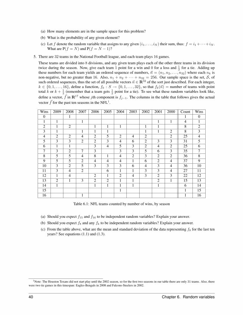
(a) How many elements are in the sample space for this problem?

(b) What is the probability of any given element?

(c) Let f denote the random variable that assigns to any given (i1, . . . , iN ) their sum, thus: f = i1 + · · ·+ iN .What are P(f = N) and P(f = N − 1)?

5. There are 32 teams in the National Football league, and each team plays 16 games.

These teams are divided into 8 divisions, and any given team plays each of the other three teams in its divisiontwice during the season. Now, give each team 1 point for a win and 0 for a loss and 1

2 for a tie. Adding upthese numbers for each team yields an ordered sequence of numbers, ~n = (n1, n2, . . . , n32) where each nk isnon-negative, but no greater than 16. Also, n1 + n2 + · · · + n32 = 256. Our sample space is the set, S, ofsuch ordered sequences, thus the set of all possible vectors ~n ∈ R32 of the sort just described. For each integer,k ∈ {0, 1, . . . , 16}, define a function, fk : S → {0, 1, . . . , 32}, so that fk(~n) = number of teams with pointtotal k or k + 1

2 (remember that a team gets 12 point for a tie). To see what these random variables look like,

define a vector, ~f in R17 whose jth component is fj−1. The columns in the table that follows gives the actualvector ~f for the past ten seasons in the NFL1.

Wins 2009 2008 2007 2006 2005 2004 2003 2002 2001 2000 Count Wins0 1 1 01 1 1 1 1 4 12 1 2 1 1 1 1 1 8 23 1 1 1 1 1 1 2 8 34 2 2 4 2 5 2 4 2 2 25 45 3 3 2 2 3 4 6 2 3 3 31 56 1 1 3 4 5 3 2 4 2 25 67 3 2 7 3 3 3 5 6 3 35 78 5 5 4 8 1 4 2 3 2 2 36 89 5 5 2 4 4 4 1 6 2 4 37 910 3 2 5 3 3 3 6 4 3 4 36 1011 3 4 2 6 1 1 3 3 4 27 1112 1 4 2 1 2 4 3 2 3 22 1213 2 1 3 2 2 1 1 2 1 15 1314 1 1 1 1 1 1 6 1415 1 1 1516 1 1 16

Table 6.1: NFL teams counted by number of wins, by season

(a) Should you expect f15 and f16 to be independent random variables? Explain your answer.

(b) Should you expect f8 and any fk to be independent random variables? Explain your answer.

(c) From the table above, what are the mean and standard deviation of the data representing f8 for the last tenyears? See equations (1.1) and (1.3).

1Note: The Houston Texans did not start play until the 2002 season, so for the first two seasons in our table there are only 31 teams. Also, therewere two tie games in this timespan: Eagles-Bengals in 2008 and Falcons-Steelers in 2002.


CHAPTER

SEVEN

The statistical inverse problem

Here is a basic issue in statistic: Experiments are often done to distinguish various hypothesis about the workings of agiven system. This is to say that you have various models that are meant to predict the behavior of the system, and youdo experiments to see which model best predicts the experimental outcomes. The ultimate goal is to use the observeddata to find the correct model.

A more realistic approach is to use the observed data to generate a probability function on the set of models thatare under consideration. The assigned probability should give the odds for the correctness of a given model. Thereare many ways to do this. Usually, any two of the resulting probability functions assign different probabilities to themodels. For this reason, if for no other, some serious thought must be given as to which (if any) to use. In any event, Idescribe some of these methods in what follows.

To indicate the flavor of what is to follow, consider first an example. Here is some background: Suppose that a givenstretch of DNA on some chromosome has N sites. If I look at this stretch in different people, I will, in general,not get the same sequence of DNA. There are typically some number of sites where the bases differ. Granted thisbasic biology, I then sample this site in a large number of people. If I find that one particular DNA sequence occursmore often then any other, I deem it to be the consensus sequence. Suppose for simplicity that there is, in fact, such aconsensus sequence. My data gives me more than just a consensus sequence; I also have numbers {p0, p1, p2, . . . , pN}where any given pk is the fraction of people whose DNA differs at k sites from the consensus sequence. For example,p0 is the fraction of people whose DNA for this N site stretch is identical to the consensus sequence. For a secondexample, p52 is the fraction of people whose DNA for this stretch differs at 52 sites from the consensus sequence.

I wish to understand how these number {p0, p1, . . . , pN} arise. If I believe that this particular stretch of DNA is ‘junkDNA’, and so has no evolutionary function, I might propose the following: There is some probability for a substitutedDNA base to appear at any given site of this N site long stretch of DNA. The simplest postulate I can make alongthese lines is that the probability of a substitution is independent of the particular site. I am interested in finding outsomething about this probability of a substitution. To simplify matters, I look for probabilities of the form m

100 wherem ∈ {0, 1, 2, . . . , 100}. So, my basic question is this:

Given the data {p0, . . . , pN}, what is the probability that a given θ = m100 is the true probability for a

single site substitution in the given stretch of DNA?

The interesting thing here is that if I know this probability, thus the number θ from the set {0, 1100 ,

2100 , . . . ,

99100 , 1},

then I can predict the sequence {p0, p1, . . . , pN}. We will give a general formula for this in a later chapter. However,for small values of N , you needn’t know the general formula as we can work things out directly.

Consider first N = 1. Then there is just p0 and p1. The probability, given θ for one site change is θ (by definition),thus the probability for no site changes is 1− θ. Hence, given θ, I would predict

Probability of 0 site changes (given θ) is 1− θ.Probability of 1 site change (given θ) is θ.

I can then compare these numbers with what I observed, p0 and p1. Doing so, I see that there is an obvious choice forθ, that with p0 = 1 − θ and p1 = θ. Of course, if I restrict θ to fractions of 100, then the I should choose the closest

41

such fraction to p1. Note, by the way, that p0 + p1 = 1 by virtue of their definition as fractions, so the two conditionson θ amount to one and the same thing.

Consider next the case N = 2. Given θ, I would then predict

Probability of 0 site changes (given θ) is (1− θ)2.Probability of 1 site change (given θ) is 2θ(1− θ). (7.1)

Probability of 2 site changes (given θ) is θ2.

To see why this is, think of flipping two coins, with heads = site change and tails = no site change; and with probabilityequal to θ for any given coin to have heads. The probability of the first coin/site having heads is θ and of it having tailsis (1− θ). Likewise for the second coin/site. So, they both end up tails with probability (1− θ)2. Likewise, they bothend up heads with probability θ2. Meanwhile, there are two ways for one head to appear, either on the first coin/site,or on the second. Each such event has probability θ(1 − θ), so the probability of one coin/site to have heads is twicethis.

This same sort of comparison with coin flipping leads to the following for the N = 3 case:

Probability of 0 site changes (given θ) is (1− θ)3.

Probability of 1 site change (given θ) is 3θ(1− θ)2.

Probability of 2 site changes (given θ) is 3θ2(1− θ). (7.2)

Probability of 3 site changes (given θ) is θ3.

However, note that in the case N = 2 the data {p0, p1, p2} need not lead to any obvious candidate for θ. This isbecause the equations

p0 = (1− θ)2 and p1 = 2θ(1− θ) and p2 = θ2

need not have a solution. Even using the fact that p0 +p1 +p2 = 1, there are still two conditions for the one unknown,θ. Consider, for example, p0 = 9

16 , p1 = 316 , p2 = 1

4 . The equations p2 = θ2 and p0 = (1− θ)2 lead to very differentchoices for θ. Indeed, the equation p2 = θ2 gives θ = 1

2 and the equation p0 = (1 − θ)2 gives θ = 14 ! This same

problem gets worse as N gets ever larger.

What’s to be done? Here is one approach: Use the data {p0, . . . , pN} to find a probability function on the possiblevalues of θ. This would be a probability function on the sample space Θ = {0, 1

100 ,2

100 , . . . ,99100 , 1} that would give

the probability for a given to be the true probability of a site substitution given the observed data {p0, . . . , pN} andgiven that my model of equal chance of a site substitution at each of the N sites along the DNA strand is correct.

I will use P to denote a probability function on Θ. This is to say that P( m100 ) is the probability that P assigns to any

given θ. For example, P( 3100 ) is the probability that 3

100 is the true probability of a mutation occurring in any givencell. Likewise, P( 49

100 ) is the probability that 49100 is the true probability of a mutation occurring in any given cell.

Imagine for the moment that I have a probability function, P , on the sample space Θ. I can then use P to make atheoretical prediction of what the observed data should be. This uses the notion of conditional probability. Here ishow it works in the case N = 2:

Prob(k site changes) = P (k | 0)P(0) + P(k | 1

100

)P( 1

100 ) + · · ·+ P (k | 1)P(1), (7.3)

where the notation uses P (k | θ) to denote the probability of there being k site changes given that θ is the correctprobability. Note that I use the conditional probability notation from Chapter 3, although the context here is slightlydifferent. Anyway, grant me this small abuse of my notation and agree to view P (k | θ) as an honest conditionalprobability. Note in this regard that it obeys all of the required rules: Each P (k | θ) is non-negative, and the sumP (0 | θ) + P (1 | θ) + · · ·+ P (N | θ) = 1 for each θ.

The key point here is that I know what these conditional probabilities P (k | θ) are. For example, they in the caseN = 2, they are given in (7.1) and in the case N = 3 they are given in (7.3). Thus, the various versions of (7.3) for

42 Chapter 7. The statistical inverse problem

N = 2 are

Prob(0 site changes) =∑

m=0,1,...100

(1− m100 )2P( m

100 )

Prob(1 site change) =∑

m=0,1,...100

2 m100 (1− m

100 )P( m100 ) (7.4)

Prob(2 site changes) =∑

m=0,1,...100

( m100 )2P( m

100 ).

Of course, I don’t yet have a probability function P . Indeed, I am looking for one; and I hope to use the experimentaldata {p0, . . . , pN} to find it. This understood, it makes some sense to consider only those versions of P that give thecorrect experimental results. This is to say that I consider as reasonable only those probability functions on the samplespace that give Prob(k site changes) = pk for all choices of k ∈ {0, . . . , N}. For example, in the case N = 2, thesegive the conditions

p0 =∑

m=0,1,...100

(1− m100 )2P( m

100 )

p1 =∑

m=0,1,...100

2 m100 (1− m

100 )P( m100 ) (7.5)

p2 =∑

m=0,1,...100

( m100 )2P( m

100 ).

To make it even more explicit, suppose again that I measured p0 = 34 , p1 = 3

16 and p2 = 116 . Then what is written

in (7.5) would read:

34 = P(0) + ( 99

100 )2P( 1100 ) + · · ·+ ( 1

100 )2P( 99100 )

316 = 2( 1

100 ) 99100 )P( 1

100 ) + 2( 2100 )( 98

100 )P( 2100 ) · · ·+ 2( 99

100 )( 1100 )P( 1

100 ) (7.6)116 = ( 1

100 )2P( 1100 ) + · · ·+ ( 99

100 )2P( 99100 ) + P(1).

Notice, by the way, that what is written here constitutes a system of 3 equations for the 101 unknown numbers,{P(0),P( 1

100 ), . . . ,P(1)}. As we know from our linear algebra, there will be infinitely many solutions. In the generalcase of a site with length N , the analog of (7.5) has N + 1 equations, with these reading

p0 =∑

m=0,1,...100

P(0 | m100

)P( m

100 )

p1 =∑

m=0,1,...100

P(1 | m100

)P( m

100 )

... (7.7)

pN =∑

m=0,1,...100

P(N | m100

)P( m

100 )

Given that I know what P (k | θ) is for any given k, this constitutes a system of N + 1 equations for the 101 unknowns{P(0),P( 1

100 ), . . . ,P(1)}. In particular, if N > 100, then there will be more equations than unknowns and so theremay be no solutions! To make this look exactly like a system of linear equation, change the notation so as to denotethe conditional probability P

(0 | m100

)as a0m, P

(1 | m100

)as a01m, etc. Use xm for P( m

100 ). And, use y0 for p0, y1 forp1, etc. This done, then (7.7) reads

y0 = a00x0 + a01x1 + · · ·y1 = a10x1 + a11x1 + · · · (7.8)

...

In any event, here is a lesson from this:

43

In general, the equations in (7.5) for the caseN = 2, or their analogs in (7.7) forN > 2 do not determinea God-given probability function on the sample space.

The task of finding a probability function on the sample space from the experimental data, one that comes reasonablyclose to solving (7.7) and makes good biological sense, is an example of what I call the statistical inverse problem.

7.1 A general setting

This sort of problem arises in the following general setting: Suppose that I am interested in some system or phenomena,and have a set, Θ, of models of how it works. I shall assume in what follows that Θ is a finite set. In the exampleoutlined above, the set Θ consists of the fractions of the form m

100 with m ∈ {0, 1, . . . , 100}. I plan to take data toexplore the phenomena. Suppose that there is a set, K, of possible experimental outcomes. In the example of theintroduction, K, consists of the numbers 0, 1, . . . , N + 1, where the integer k here denotes the number of sites on thegiven N -site DNA strand that differ from the consensus strand. Even in the general case, if there are but a finite set ofpossible outcomes, I can label them by consecutive integers starting from zero and this I now do.

As I know a competent model builder, I make sure that each model from Θ determines a probability function on K.This is to say any given model θ ∈ Θ gives a predicted probability for any given outcome in K. I write θ’s versionof the probability of the kth outcome as P (k | θ). Thus, P (k | θ) is the probability of having the kth outcome wereθ the correct model. In the N = 2 example from the introduction, P (0 | θ) = (1 − θ)2, P (1 | θ) = 2θ(1 − θ) andP (2 | θ) = θ2.

I take lots of data and so generate an experimentally determined probability function, Pexp, on K. Here, Pexp(k) is thefraction of the experiments where kth outcome appeared. In the example from the introduction, the number Pexp(k)is what I called pk.

The statistical inverse problem in this context is as follows: Use the experimentally determined probability functionPexp to determine a probability function, P , on the set Θ. You are asked to use what you know, the data derivedfrequencies Pexp and the set of conditional probabilities, the various P (k | θ), to find those model parameters from Θthat are more likely to be correct, and which are less likely to be correct.

Keep in mind that there is, in general, no God-given way to generate a probability function on the set Θ. Even so,there are various popular methods and one or more may well be useful in any given context.

7.2 The Bayesian guess

The Bayesian turns things upside down and reasons is as follows: Suppose that I have a conditional probability thattells me the probability that the model labeled by θ is correct given that the kth outcome in K appears. Suppose Ihave such a conditional probability for each outcome k and each parameter θ. I use P (θ | k) to denote this conditionalprobability. If I had such a collection of conditional probabilities, then I could use the general form of Bayes’ theoremin (3.5) to write a probability function on the set Θ. This would be the function whose value on any given θ is

P(θ) = P (θ | 0) Pexp(0) + P (θ | 1) Pexp(1) + · · ·+ P (θ |N) Pexp(N) (7.9)

In our N = 2 case from the introduction, there are 101 versions of (7.9), one for each fraction { m100}m=0,1,...100, andthe mth version reads

P( m100 ) = P

(m

100 | 0)

Pexp(0) + P(m

100 | 1)

Pexp(1) + P(m

100 | 2)

Pexp(2) (7.10)

Of course, this is wishful thinking without some scheme to obtain the various conditional probabilities P (θ | k).

The Bayesian makes the following rather ad-hoc proposal: Let’s use for P the formula

PBayes (θ | k) = P(k | θ)Z(k) (7.11)


where Z(k) =∑θ∈Θ P (k | θ) is needed so that the PBayes (θ | k) can be interpreted as a conditional probability.

The point here is that the probability of some θ happening given k is 1, so with any k fixed, the sum of the variousPBayes (θ | k) for all of the θ in Θ has to be 1. This is guaranteed with the factor 1

Z(k) present, but may not be the casewithout this factor. Using PBayes in (7.9) gives what is called the Bayesian version of a probability function on Θ:

PBayes(θ) = P (0 | θ) 1Z(0) Pexp(0) + P (1 | θ) 1

Z(1) Pexp(1) + · · · . (7.12)

Note that the presence of Z guarantees that the probabilities defined by the left-hand side of (7.12) sum to 1.

In effect, the Bayesian probability function on Θ is obtained by approximating the unknown conditional probabilityfor θ given outcome k by the known conditional probability of outcome k given θ (times the factor 1

Z(k) ). This mayor may not be a good approximation. In certain circumstances it is, and in others, it isn’t.

7.3 An example

To see how this works in an example, consider theN = 2 case of the introduction. In this case, θ is one of the fractionsfrom the set Θ = { m100}m=0,1,...100 and (7.1) finds that P (0 | θ) = (1− θ)2, P (1 | θ) = 2θ(1− θ) and P (2 | θ) = θ2.This understood, then

Z(0) = 1 + ( 99100 )2 + ( 98

100 )2 + · · ·+ ( 1100 )2 ≈ 33.835

Z(1) = 2( 1100 )( 99

100 ) + 2( 98100 )( 2

100 ) + · · ·+ 2( 99100 )( 1

100 ) ≈ 33.33 (7.13)

Z(2) = ( 1100 )2 + ( 2

100 )2 + · · ·+ 1 ≈ 33.835.

Using this in (7.12) gives the Bayesian probability function whose value on m100 is

PBayes( m100 ) = (1− m

100 )2 133.835p0 + 2( m

100 )(1− m100 ) 1

33.33p1 + ( m100 )2 1

33.835p2. (7.14)

For example, if it turned out that p0 = 34 , p1 = 3

16 and p2 = 116 , then the Bayesian guess for a probability function

would bePBayes( m

100 ) = (1− m100 )2 1

33.83534 + 2( m

100 )(1− m100 ) 1

33.33316 + ( m

100 )2 133.835

116 .

Assume that you calculate PBayes in a given situation. You must then ask: What in the world does it tell me about myset of possible models? It gives a probability function on this set, but so what. There are lots of probability functionson any given set. The fact is that before you use PBayes (or any of other version of P), you need to think long and hardabout whether it is really telling you anything useful.

By the way, the formula in (7.14) for PBayes is another disguised version of what we are doing in linear algebra (as isthe formula in (7.12)). To unmask this underlying linear algebra, agree to change to the linear algebra book’s notationand so use x0 to denote p0, use x1 to denote p1 and x2 to denote p2. Then use ym to denote P( m

100 ) and use am1 todenote the number (1− m

100 )2, use am2 to denote 2( m100 )(1− m

100 ) and am3 to denote ( m100 )2. This done, then the 101

versions of (7.14) read

y0 = a00x0 + a01x1 + a02x2

y1 = a10 x0 + a11 x1 + a12x2

· · · etc.

7.4 Gregor Mendel’s peas

What follows gives another example of how the statistical inverse problem can arise. This involves a classic experimentdone by Gregor Mendel. For those unfamiliar with the name, here is part of what Wikipedia has to say about Mendel(http://en.wikipedia.org/wiki/Mendel):

7.3. An example 45

http://en.wikipedia.org/wiki/Mendel

Gregor Johann Mendel (July 20[1], 1822 – January 6, 1884) was an Augustinian abbot who is often calledthe “father of modern genetics” for his study of the inheritance of traits in pea plants. Mendel showedthat the inheritance of traits follows particular laws, which were later named after him. The significanceof Mendel’s work was not recognized until the turn of the 20th century. Its rediscovery prompted thefoundation of genetics.

What follows describes the experiment: A given pea plant, when self-pollinated, can have either round or angularseeds. It can also have either yellow or green seeds. Mendel took 10 plants, where each plant can have either round orangular seeds, and either yellow or green seeds. Each plant was self-pollinated, and Mendel kept track of the numberof seeds that were round and the number that were angular. He also kept track of the number that were yellow and thenumber that were green. Here are the published results (from http://www.mendelweb.org/Mendel.html):

Experiment 1 Experiment 2(Shape) (Color)

Plant # Round Angular Yellow Green1 45 12 25 112 27 8 32 73 24 7 14 54 19 10 70 275 32 11 24 136 26 6 20 67 88 24 32 138 22 10 44 99 28 6 50 14

10 25 7 44 18Totals 336 101 355 123

Using the totals at the bottom finds that round seeds appear 77% of the time. Meanwhile, yellow seeds appear 74%of the time. Let us agree to use pr = 0.77 for the experimentally determined probability for a seed to be round, andpy = 0.74 for the experimentally determined probability for a seed to be yellow.

The conventional wisdom explains the numbers of round and angular seeds by postulating that each plant has twodifferent genes that convey instructions for seed shape. These are denoted here by ‘R’ (for round) and ‘a’ (for angular).The parent in each case is hypothesized to be type Ra. The offspring inherits either type RR, Ra or aa, where one ofthe genes, either R or a, comes from the pollen and the other from the ovule. The hypothesis is that R is dominant sotypes RR and Ra come from round seeds. Meanwhile, offspring of type aa come from angular seeds.

There is a similar story for the color of the seed. Each plant also has two genes to control seed color. These are denotedhere by ‘Y’ and ‘g’. The parent is type Yg, and the offspring can be of type YY, Yg or gg. The Y is postulated to bethe dominant of the two genes, so offspring of type YY or Yg have yellow seeds, while those of type gg have roundseeds.

The conventional wisdom assigns probability 12 for any given pollen grain or ovule to receive the dominant gene for

shape, and likewise probability 12 to receive the dominant gene for color. One should make it a habit to question

conventional wisdom! In particular, suppose that we wish to compare the conventional probability model with anothermodel, this giving some probability, θ, for any given pollen grain or ovule to have the dominant allele. To keep thingssimple, I will again assume that θ can be any number { m100}m∈{0,1,...,100}. In this case, our set of models is again the101 element set Θ = { m100}m∈{0,1,...100}.

7.5 Another candidate for P(θ): A maximum likelihood candidate.

What follows describes a simplistic thing that can be done with the data so as to determine a probability function onΘ. Look again at Mendel’s data. In a sense, 915 different experiments are represented in this table, one for each



seedling with regards to round versus angular seed, and one from each seed with regards to yellow versus green color.To see how to make sense of this, consider a sample space S with 2915 elements, where each element is a vector inR915 whose entries are either 0 or 1. Each entry represents one of the 915 possible outcomes for the round/angularand yellow/green traits. The value 0 occurs in any given entry if the recessive trait is present, and the value 1 occursif the dominant trait is present. Each θ ∈ { m100}m∈{0,...100} gives us a probability function on this sample space S.For example, the probability that there all 915 cases have the recessive trait is ((1 − θ)2)915, and the probability thatall have the dominant trait is (2θ − θ2)915. Thus, when θ = 1

2 , the vector in S with all 915 entries equal to 0 hasprobability ( 1

4 )915, and the vector in S with all 915 entries equal to 1 has probability ( 34 )915. Here is how to think

of this probability function: Imagine flipping a coin 915 times keeping track of the number of heads and the numberof tails; here the coin is biased so that a head appears with probability (2θ − θ2) and a tail appears with probability(1− θ)2. You are asked in a homework problem how to compute the probability of any given element in S.

Consider next the following random variable on S: Suppose that a = (a1, . . . , a915) ∈ S. Set f(a) to be the sum ofthe entries. Thus, f(a) = a1 + a2 + · · ·+ a915. This is the total number of dominant traits that appear if the vector arepresents the outcome of the 915 experiments. For example, a vector in S that gives Mendel’s data, the value of f is691.

Now, as remarked above, each θ from Θ determines a probability function on S. As described in the previous chapter,such a probability function on S can be used to obtain a probability function on the set of possible values for therandom variable f . This set is the set of integers starting at 0 and ending at 915. Let me use Pf (k | θ) to denote theprobability function on the set {0, 1, . . . , 915} that is determined by θ. Said differently, if k ∈ {0, 1, . . . , 915}, thenPf (k | θ) is the probability as determined by θ of the set of elements in S whose entries sum to k. This can be viewedas a sort of conditional probability for f to equal k given that θ is the parameter used to determine the probabilities onS. This is why I use the notation Pf (k | θ). Upcoming chapters will give us the tools to compute Pf (k | θ). For now,just imagine this to be some function on the set {0, 1, . . . , 915} whose values are non-negative and sum up to 1.

If, for a given θ, the probability Pf (691 | θ) is small relative to other values of θ, then this particular value of θ shouldhave small probability of being correct. If, for a given θ, the probability Pf (691 | θ) is large relative to others, thenI might expect that this particular θ should have greater probability of being true. These observations motivate theintroduction of the following probability function on the set Θ:

PML(θ) = Pf (691 | θ) /Z where Z =∑

m=0,1,2,...100

Pf(691 | m100

). (7.15)

Note that the factor of Z = Pf (691 | 0) + Pf(691 | 1

100

)+ · · · + Pf (691 | 1) is necessary so as to guarantee that

the sum of the values of PML over all 101 elements in Θ is equal to 1. What is written in (7.15) is called by some amaximum likelihood probability function on the set Θ.

Of course, this is all pretty abstract if Pf (691 | θ) can’t be computed. As we shall see in an upcoming chapter, it is, infact, computable:

Pf (691 | θ) =915× 914× · · · × 1

(224× 223× · · · × 1) (691× 690× · · · × 1)(2θ − θ2)691((1− θ)2)224. (7.16)

In any event, this probability function assigns the greatest probability to the model whose version of Pf (691 | θ) islargest amongst all models under consideration. This is to say that the model that PML makes most probable is the onethat gives the largest probability to the number 691.

To see this approach in a simpler case, suppose that instead of 915 seedlings, I only had 4, and suppose that three ofthe four exhibited the dominant trait, and one of the four exhibited the recessive trait.

My sample space S for this simple example consists of 24 = 16 elements, these

• (0, 0, 0, 0)• (1, 0, 0, 0), (0, 1, 0, 0), (0, 0, 1, 0), (0, 0, 0, 1)• (1, 1, 0, 0), (1, 0, 1, 0), (1, 0, 0, 1), (0, 1, 1, 0), (0, 1, 0, 1), (0, 0, 1, 1) (7.17)• (1, 1, 1, 0), (1, 1, 0, 1), (1, 0, 1, 1), (0, 1, 1, 1)• (1, 1, 1, 1).

7.5. Another candidate for P(θ): A maximum likelihood candidate. 47

To simplify the notation, set α = (1 − θ)2. This is the probability of seeing the recessive trait for the model whereθ ∈ { m100}m∈{0,1,...,100} gives the probability that any given pollen grain or ovule has the dominant allele. Thus,(1 − α) is the probability of seeing the dominant trait given the value of θ. For example, α = 1

4 when θ = 12 . In any

event with θ given, then the probability function on S that is determined by θ gives the following probabilities:

P = α4 to (0, 0, 0, 0)

P = α3(1− α) to everything in the second row of (7.17)

P = α2(1− α)2 to everything in the third row of (7.17) (7.18)

P = α(1− α)3 to everything in the fourth row of (7.17)

P = (1− α)4 to (1, 1, 1, 1).

(You are asked to justify (7.18) in a homework problem.)

In this baby example, the possible values of f are {0, 1, 2, 3, 4}, and the set of elements in S that give the value f = kconsists of the kth row in (7.17). This being the case, then

Pf (0 | θ) = α4, Pf (1 | θ) = 4α3(1− α), Pf (2 | θ) = 6α2(1− α)2,

Pf (3 | θ) = 4α(1− α)3, Pf (2 | θ) = (1− α)4.

In particular, Pf (3 | θ) = 4α(1− α)3. In terms of θ, this says that Pf (3 | θ) = 4(1− θ)2(2θ − θ2)3.

The analog of (7.10) for this example sets

PML(θ) = 120.31754(1− θ)2(2θ − θ2)3. (7.19)

In this case Z = 20.3175. I’ll leave it as an exercise for those who remember their one variable calculus to verify thatthe function θ → P(θ) has its maximum at θ = 1

2 .

As with the Bayesian probability function, you must still ask yourself whether the assigned probabilities to the modelsare useful or not. For example, the probability function in (7.19) finds PML( 1

2 ) ≈ 0.02. Meanwhile, PML( 23 ) ≈ 0.015.

Is it really the case that the probabilities for θ = 12 and θ = 2

3 should be so nearly equal? The fact is that theseprobabilities are close is due to the fact that the data from 4 seedlings is not nearly enough to distinguish these twomodels. This is what I meant when I said at the outset that you must think hard about whether any probability functionon your set of possible models is worth looking at. The fact that these two probabilities are so close really says nothingabout peas and genetics, and everything about the fact that you don’t have enough data to discriminate.

This gets to the heart of the matter with regards to using statistics: A good deal of common sense must be used tointerpret the mathematics.

7.6 What to remember from this chapter

This has been somewhat of a rambling chapter, so I thought to tell you what are the important things to keep in mind:

• A fundamental purpose of statistics is to provide tools that allow exper-imental data to assign probabilities to various proposed models for pre-dicting the outcomes of the experiment.

• There are many such tools. (7.20)

• Depending on the circumstances, some of these tools will be more use-ful than others. In particular, some techniques can give misleading ornonsensical conclusions.

Later chapters introduce other methods of assessing whether a given experimental model is likely to be valid. However,in using any such technique, it is important to keep your wits about you – use common sense and your understandingof the experimental protocol to decide whether a given statistical technique will be useful or not. Always remember:


Mathematics can’t turn processed pig feed into gold.

The point is that the your data may not be sufficiently powerful to distinguish various models; and if this is the case,then no amount of fancy mathematics or statistics is going to provide anything useful.

7.7 Exercises:

1. Suppose that the probability that any given pollen grain or ovule has the recessive allele is some number α ∈[0, 1], and so the probability that either has the dominant gene is (1− α).

(a) Consider an experiment where 4 seedlings are examined for the dominant or recessive trait. Thus, theoutcome of such an experiment is a vector in R4 whose kth entry is 0 if the kth seedling has the recessivetrait and it is 1 if the kth seedling has the dominant trait. Let S denote the 24 = 16 element set of possibleexperimental outcomes. Let s ∈ S denote an element with some m ∈ {0, . . . , 4} entries equal to 1 and theremaining entries equal to zero. Explain why s has probability (1− α)mα4−m.

(b) Consider now the analogous experiment where 915 seedlings are examined for the dominant or recessivetrait. Thus, the outcome of such an experiment is a vector in R915 whose kth entry is 0 if the kth seedlinghas the recessive trait and it is 1 if the kth seedling has the dominant trait. Let S denote the 2915 elementset of possible experimental outcomes. Let s ∈ S denote an element with some m ∈ {0, . . . , 915} entriesequal to 1 and the remaining entries equal to zero. Explain why the m has probability (1− α)mα915−m.

(c) In the case of part (a) above, define the random variable f : S → {0, 1, 2, 3, 4} where f(s) is the sum ofthe entries of s. Compute the induced probability function Pf on the set {0, 1, 2, 3, 4}.

7.7. Exercises 49

CHAPTER

EIGHT

Kernel and image in biology

Imagine a complicated cellular process that involves some n genes that are presumably ‘turned on’ by some N othergenes that act at an earlier time. We want to test whether the effect of the early genes on the late genes involves acomplicated synergy, or whether their affects simply add. To do this, I could try to derive the consequences of oneor the other of these possibilities and then devise an experiment to see if the predicted consequences arise. Such anexperiment could vary the expression level of the early genes from their normal levels (either + or −) and see how thevariation in the level of expression of the late genes from their normal levels changes accordingly.

To elaborate on this strategy, note that when a gene is expressed, its genetic code (a stretch of the DNA molecule) isused to code for a molecule much like DNA called mRNA. Here, the ‘m’ stands for ‘messenger’ and the RNA part isa sequence of small molecules strung end to end. Any of these can be one of four and the resulting sequence along theRNA string is determined by the original sequence on the coding stretch of DNA. This messenger RNA subsequentlyattaches to the protein making part of a cell (a ‘ribosome’) where its sequence is used to construct a particular proteinmolecule. In any event, the level of any given mRNA can be measured at any given time, and this level serves as aproxy for the level of expression of the gene that coded it in the first place.

One more thing to note: The level of expression of a gene can often be varied with some accuracy in an experiment byinserting into the cell nucleus certain tailored molecules to either promote or repress the gene expression. Such is themagic of modern biotechnology.

To make a prediction that is testable by measuring early and late gene expression, let us suppose that the affects ofthe early genes are simply additive and see where this assumption leads. For this purpose, label these early genesby integers from 1 to N , and let uk to denote the deviation, either positive or negative, of the level of expression ofthe kth early gene from its normal level. For example, we can take uk to denote the deviation from normal of theconcentration of the mRNA that comes from the kth early gene.

Meanwhile, label the late genes by integers from 1 to n, and use pj to denote the deviation of the latter’s mRNA fromits normal level. If the affects of the early genes on the late genes are simply additive, we might expect that any givenpj has the form

pj = Aj1u1 +Aj2u2 + · · ·+AjNuN , (8.1)

where each Ajk is a constant. This is to say that the level pj is a sum of factors, the first proportional to the amountof the first early gene, the second proportional to the amount of the second early gene, and so on. Note that whenAjk is positive, then the kth early gene tends to promote the expression of the jth late gene. Conversely, when Ajk isnegative, the kth early gene acts to repress the expression of the jth late gene.

If we use ~u to denote the N -component column vector whose kth entry is uk, and if we use ~p to denote the n-component column vector whose jth component is pj , then the equation in (8.1) is the matrix equation ~p = A~u. Thus,we see a linear transformation from an N -dimensional space to an n-dimensional one.

By the way, note that the relation predicted by (8.1) can, in principle, be tested by experiments that vary the levels ofthe early genes and see if the levels of the late genes change in a manner that is consistent with (8.1). Such experimentswill also determine the values for the matrix entries {Ajk}. For example, to find A11, vary u1 while keeping all k > 1versions of uk equal to zero. Measure p1 as these variations are made and see if the ratio p1/u1 is constant as u1

changes with each k > 1 version of uk equal zero. If so, the constant is the value to take for A11. If this ratio is not

50

constant as these variations are made, then the linear model is wrong. One can do similar things with the other pj anduk to determine all Ajk. One can then see about changing more than one uk from zero and see if the result conformsto (8.1).

The question now arises as to the meaning of the kernel and the image of the linear transformation A from RN to Rn.To make things explicit here, suppose that n and N are both equal to 3 and that A is the matrix

A =

1 1 22 1 11 0 −1

(8.2)

As you can check, this matrix has kernel equal to the scalar multiples of the vector 1−31

(8.3)

Meanwhile, its image is the span of the vectors011

and

110

. (8.4)

Thus, it consists of all vectors in R3 that can be written as a constant times the first vector in (8.4) plus another constanttimes the second.

Here is the meaning of the kernel: Vary the early genes 1, 2 and 3 from their normal levels in the ratio u1/u3 = 1and u2/u3 = −3 and there is no affect on the late genes. This is to say that if the expression levels of early genes 1and 3 are increased by any given amount r while that of early gene 2 is decreased by 3r, then there is no change tothe levels of expression of the three late genes. In a sense, the decrease in the level by a factor of 3 of the second earlygene exactly offsets the affect of increasing the equal increases in the levels of the first and third early genes.

As to the meaning of the image, what we find is that only certain deviations of the levels of expression of the three lategenes from their background values can be obtained by modifying the expression levels of the three early genes. Forexample, both vectors in (8.4) are orthogonal to the vector 1

−11

. (8.5)

Thus, values of p1, p2 and p3 with the property that p1 +p3 6= p2 can not be obtained by any variation in the expressionlevels of the three early genes. Indeed, the dot product of the vector ~p with the vector in (8.5) is p1 − p2 + p3 and thismust be zero in the case that is a linear combination of the vectors in (8.4).

Granted that the matrix A is that in (8.2), then the preceding observation has the following consequence for thebiologist: If values of p1, p2 and p3 are observed in a cell with p1 + p3 6= p2, then the three early genes can not be thesole causative agent for the expression levels of the three late genes.

51

CHAPTER

NINE

Dimensions and coordinates in a scientificcontext

My purpose here is to give some toy examples where the notion of dimension and coordinates appear in a biologicalcontext.

9.1 Coordinates

Here is a hypothetical situation: Suppose that a cell has genes labeled {1, 2, 3}. The level of the corresponding productthen defines vector in R3 where the obvious coordinates, x1, x2 and x3, measure the respective levels of the productsof gene 1, gene 2 and gene 3. However, this might not be the most useful coordinate system. In particular, if somesubsets of genes are often turned on at the same time and in the same amounts, it might be better to change to a basiswhere that subset gives one of the basis vectors. Suppose for the sake of argument, that it is usually the case that thelevel of the product from gene 2 is three times that of gene 1, while the level of the product of gene 3 is half that ofgene 1. This is to say that one usually finds x2 = 3x1 and x3 = x1. Then it might make sense to switch from thestandard coordinate bases,

~e1 =

100

, ~e2 =

010

, ~e3 =

001

, (9.1)

to the coordinate system that uses a basis ~v1, ~v2 and ~v3 where

~v1 =

1312

, ~v2 = ~e2, ~v3 = ~e3. (9.2)

To explain, suppose I measure some values for x1, x2 and x3. This then gives a vector,

~x =

x1

x2

x3

= x1~e1 + x2~e2 + x3~e3. (9.3)

Now, I can also write this vector in terms of the basis in (9.2) as

~x = c1~v1 + c2~v2 + c3~v3. (9.4)

With ~v1, ~v2 and ~v3 as in (9.2), the coordinates c1, c2 and c3 that appear in (9.5) are

c1 = x1, c2 = x2 − 3x1, and c3 = x3 − x1. (9.5)

As a consequence, the coordinates c2 describes the deviation of x2 from its usual value of 3x1. Meanwhile, thecoordinate c3 describes the deviation of x3 from its usual value of x1.

52

Here is another example: Suppose now that there are again three genes with the levels of their corresponding productsdenoted as x1, x2, and x3. Now suppose that it is usually the case that these levels are correlated in that x3 is generallyvery close to 2x2 + x1. Any given set of measured values for these products determines now a column vector asin (9.3). A useful basis in this case would by one where the coordinates c1, c2 and c3 has

c1 = x1, c2 = x2, and c3 = x3 − 2x2 − x1. (9.6)

Thus, c3 again measures the deviation from the expected values. The basis with this property is that where

~v1 =

101

, ~v2 =

012

, and ~v3 =

001

. (9.7)

This is to say that if ~v1, ~v2, and ~v3 are as depicted in (9.7), and if ~x is then expanded in this basis as c1~v1 +c2~v2 +c3~v3,then c1, c2 and c3 are given by (9.6).

9.2 A systematic approach

If you are asking how I know to take the basis in (9.7) to get the coordinate relations in (9.6), here is the answer:Suppose that you have coordinates x1, x2 and x3 and you desire new coordinates, c1, c2 and c3 that are related to thex’s by a linear transformation: c1c2

c3

= A

x1

x2

x3

, (9.8)

where A is an invertible, 3 × 3 matrix. In this regard, I am supposing that you have determined already the matrix Aand are simply looking now to find the vectors ~v1, ~v2 and ~v3 that allow you to write ~x = c1~v1 + c2~v2 + c3~v3 with c1,c2 and c3 given by (10.8). As explained in the linear algebra text, the vectors to take are:

~v1 = A−1~e1, ~v2 = A−1~e2, ~v3 = A−1~e3. (9.9)

To explain why (9.9) holds, take the equation ~x = c1~v1 +c2~v2 +c3~v3 and act on both sides by the linear transformationA. According to (9.8), the left-hand side, A~x, is the vector ~c whose top component is c1, middle component is c2 andbottom component is c3. This is to say that A~x = c1~e1 + c2~e2 + c3~e3. Meanwhile, the left-hand side of the resultingequation is c1A~v1 + c2A~v2 + c3A~v3. Thus,

c1~e1 + c2~e2 + c3~e3 = c1A~v1 + c2A~v2 + c3A~v3. (9.10)

Now, the two sides of (9.10) are supposed to be equal for all possible values of c1, c2 and c3. In particular, they areequal when c1 = 1 and c2 = c3 = 0. For these choices, the equality in (9.10) asserts that ~e1 = A~v1; this the left-mostequality in (9.9). Likewise, setting c1 = c3 = 0 and c2 = 1 in (9.10) gives the equivalent of the middle equalityin (9.9); and setting c1 = c2 = 0 and c3 = 1 in (9.10) gives the equivalent of the right-most equality in (9.9).

9.3 Dimensions

What follows is an example of how the notion of dimension arises in a scientific context. Consider the situation inSection 9.1, above, where the system is such that the levels of x2 and x3 are very nearly x2 ≈ 3x1 and x3 ≈ x1. Thisis to say that when we use the coordinate c1, c2 and c3 in (9.5), then |c2| and |c3| are typically very small. In this case,a reasonably accurate model for the behavior of the three gene system can be had by simply assuming that c2 andc3 are always measured to be identically zero. As such, the value of the coordinate c1 describes the system to greataccuracy. Since only one coordinate is needed to describe the system, it is said to be ‘1-dimensional’.

A second example is the system that is described by c1, c2 and c3 as depicted in (9.6). If it is always the case that x3

is very close to 2x2 + x1, then the system can be described with good accuracy with c3 set equal to zero. This done,

9.2. A systematic approach 53

then one need only specify the values of c1 and c2 to describe the system. As there are two coordinates needed, thissystem would be deemed ‘2-dimensional’.

In general, some sort of time dependent phenomena is deemed ‘n-dimensional’ when n coordinates are required todescribe the behavior to some acceptable level of accuracy. Of course, it is typically the case that the value of ndepends on the desired level of accuracy.

9.4 Exercises:

1. Suppose that four genes have corresponding products with levels x1, x2, x3 and x4 where x4 is always veryclose to x1 + 4x2 while x3 is always very close to 2x1 + x2. Find a new set of basis vectors for R4 andcorresponding coordinates c1, c2, c3 and c4 with the following property: The values of x1, x2, x3 and x4 forthis four gene system are the points in the (c1, c2, c3, c4) coordinate system where c3 and c4 are nearly zero.

2. Suppose that two genes are either ‘on’ of ‘off’, so that there are affectively, just four states for the two genesystem, {++,+−,−+,−−}, where ++ means that both genes are on; +− means that the first is on and thesecond is off; etc. Assume that these four states have respective probabilities 1

2 , 16 , 1

6 , 16 .

(a) Is the event that the first gene is on independent from the event that the second gene is on?

Now suppose that these two genes jointly influence the levels of two different products. The levels of the firstproduct are given by {3, 2, 1, 0} in the respective states ++, +−, −+, −−. The levels of the second are{4, 2, 3, 1} in these same states.

(b) View the levels of the two products as random variables on the sample space S that consists of{++,+−,−+,−−} with the probabilities as stated. Write down the mean and standard deviations forthese two random variables.

(c) Compute the correlation matrix in equation (6.8) of Chapter 6 for these two random variables to prove thatthey are not independent.

54 Chapter 9. Dimensions and coordinates in a scientific context

CHAPTER

TEN

More about Bayesian statistics

The term ‘Bayesian statistics’ has different meanings for different people. Roughly, Bayesian statistics reverses‘causes’ and ‘effects’ so as to make an educated guess about the causes given the known effects. The goal is de-duce a probability function on the set of possible causes granted that we have the probabilities of the various effects.

Take note that I have underlined the words ‘educated guess’. There are situations when the Bayesian strategy seemsreasonable, and others where it doesn’t.

10.1 A problem for Bayesians

There is a sample space of interest, S, with a known function (i.e. random variables) f to another finite set, W . Aprobability function for the set W is in hand, but what is needed is one for the set S.

Here is a simple situation that exemplifies this: Flip two distinct coins, coin #1 and coin #2. Move to the right one step(x → x + 1) for each heads that appears and to the left one step (x → x − 1) for each tails. Let W denote the set ofpossible positions after two flips, thus W = {−2, 0, 2}. Meanwhile, the sample space is S = {HH,HT, TH, TT}.We can do this experiment many times and so generate numbers Pexp(−2), Pexp(0) and Pexp(2) that give the respectivefrequencies that−2, 0 and 2 are the resulting positions. How can we use these frequencies to determine the probabilityof getting heads on coin #1, and also the probability of getting heads on coin #2? In this regard, we don’t want toassume that these coins are fair, nor do we want to assume that the probability of heads for coin #1 is the same as thatfor coin #2.

10.2 A second problem

A six-sided die, hidden from view, is rolled twice and the resulting pair of numbers (each either 1, 2, . . ., 6) are addedto obtain a single number, thus an integer that can be as small as 2 or as large as 12. We are told what this sum is, butnot the two integers that appeared. If this is done many times, how can the relative frequencies for the various valuesof the sum be used to determine a probability function for the sample space?

10.3 Meet the typical Bayesian

To set the stage, remember that if P is any given probability function on S, then P induces one on W by the rule wesaw in Chapter 5. Indeed, if the latter is denoted by Pf , the rule is that Pf (r) is the probability as measured by P of thesubset of points in S where f has value r. Thus,

Pf (r) =∑

s∈S with f(s)=r

P(s). (10.1)

55

This last equation can be written in terms of conditional probabilities as follows:

Pf (r) =∑s∈S

P (r | s) P(s) (10.2)

where P (r | s) is the conditional probability that f = r given that you are at the point s ∈ S. Of course, this just saysthat P (r | s) is 1 if f(s) = r and 0 otherwise.

The problem faced by statisticians is to deduce P, or a reasonable approximation, given only knowledge of somepreviously determined probability function, PW , on the set W . In effect, we want to find a probability function P onS whose corresponding Pf is the known function PW .

Your typical Bayesian will derive a guess for P using the following strategy:

Step 1: Assume that there is some conditional probability, K(s; r), that gives the probability of obtaining any givens from S granted that the value of f is r. If such a suite of conditional probabilities were available, then one couldtake

Pguess(s) =∑r∈W

K(s; r)PW (r). (10.3)

The problem is that the points in W are the values of a function of the points in S, not vice-versa. Thus, there is oftenno readily available K(s; r).

Step 2: A Bayesian is not deterred by this state of affairs. Rather, the Bayesian plows ahead by using what we have,which is P (r | s). We know its values in all cases; it is 1 when f(s) = r and zero otherwise. Why not, asks theBayesian, take

K(s; r) =1

Z(r)P (r | s) , (10.4)

where Z(r) is the number of points in S on which f has value r. This, is to say that

Z(r) =∑s∈S

P (r | s) . (10.5)

To explain the appearance of Z(r), remember that a conditional probability of the form P (A |B) is a probabilityfunction in its own right on the sample space S. Thus, P (S |B) must be 1 if S is the whole sample space. This neednot be the case for K(S; r) were the factor of 1/Z(r) absent.

Step 3: To summarize: Our typical Bayesian takes the following as a good guess for the probability function on S:

PBayes(s) =∑r∈W

1Z(r)

P (r | s) PW (r). (10.6)

Note that disentangling the definitions, there is really no summation involved in (10.6) because there is just one valueof r that makes P (r | s) non-zero for any given s, this the value r = f(s). Thus, (10.6) is a very roundabout way ofsaying that

PBayes(s) =1

Z(f(s))PW (f(s)). (10.7)

This is our Bayesian’s guess for the probability function on S.

10.4 A first example

Consider the problem in Part a with flipping coin #1 and coin #2. As noted there, W denotes the set of possiblepositions after the two coin flips, thus W = {−2, 0, 2}. The set S = {HH,HT, TH, TT}. Suppose first that our

56 Chapter 10. More about Bayesian statistics

two coins have the same probability for heads, some number q ∈ (0, 1). Thus T has probability 1 − q, then the trueprobabilities for the elements in S are q2, q(1 − q), q(1 − q) and (1 − q)2 in the order they appear above. Theseprobability assignments give Ptrue on S. With these true probabilities, the frequencies of appearances of the threeelements in W are (1− q)2, 2q(1− q) and q2. I’ll take these for my definition of the probability function PW on W .

Let’s now see what the Bayesian would find for PBayes. For this purpose, note that the only non-zero values of P (r | s)that appear in the relevant version of (9.6) are

• P(−2, TT ) = 1

• P(0, HT ) = P(0, TH) = 1

• P(2, HH) = 1

(10.8)

Thus, Z(±2) = 1 and Z(0) = 2. Plugging this into (10.7) finds

PBayes(HH) = q2, PBayes(TT ) = (1− q)2 and PBayes(HT ) = PBayes(TH) = q(1− q). (10.9)

Thus, the Bayesian guess for probabilities is the true probability.

10.5 A second example

Let us now change the rules in the coin flip game and consider the case where the first flip uses a fair coin (probability12 ) for either H or T , and the second uses a biased coin, with probability q for H and thus (1− q) for T . In this case,the true probability on S is given by

Ptrue(HH) = 12q, Ptrue(HT ) = 1

2 (1− q), Ptrue(TH) = 12q, and Ptrue(TT ) = 1

2 (1− q). (10.10)

The frequencies of appearance of the three positions in W are now 12 (1− q), 1

2 , 12q. I use these three numbers for the

probabilities given by PW . As the conditional probabilities in (10.8) do not change, we can employ then in (10.6) tofind the Bayesian guess:

PBayes(HH) = 12q, PBayes(HT ) = 1

4 , PBayes(TH) = 14 , and PBayes(TT ) = 1

2 (1− q). (10.11)

Thus, the Bayesian guess goes bad when q deviates from 12 .

Roughly speaking, the Bayesian guess cannot distinguish between those points in the sample space that give the samevalue for random variable f .

10.6 Something traumatic

Let me show you something that is strange about the Bayesian’s guess in (10.11). Suppose we ask for the probabilityas computed by PBayes that H appears on the first coin. According to our rules of probability,

PBayes(coin #1 = H) = PBayes(HH) + PBayes(HT ) = 12q + 1

4 . (10.12)

This is also the probability PBayes(coin #2 = H) since PBayes(HT ) = PBayes(TH). Now, note that

PBayes(HH) 6= PBayes(coin #1 = H)PBayes(coin #2 = H) (10.13)

unless q = 12 since the left-hand side is 1

2q and the right is ( 12q + 1

4 )2. Thus, the Bayesian finds that the event ofcoin #1 = H is not independent of the event that coin #2 = H!! (Remember that events A and B are deemedindependent when P(A ∩B) = P(A)P(B).)

10.5. A second example 57

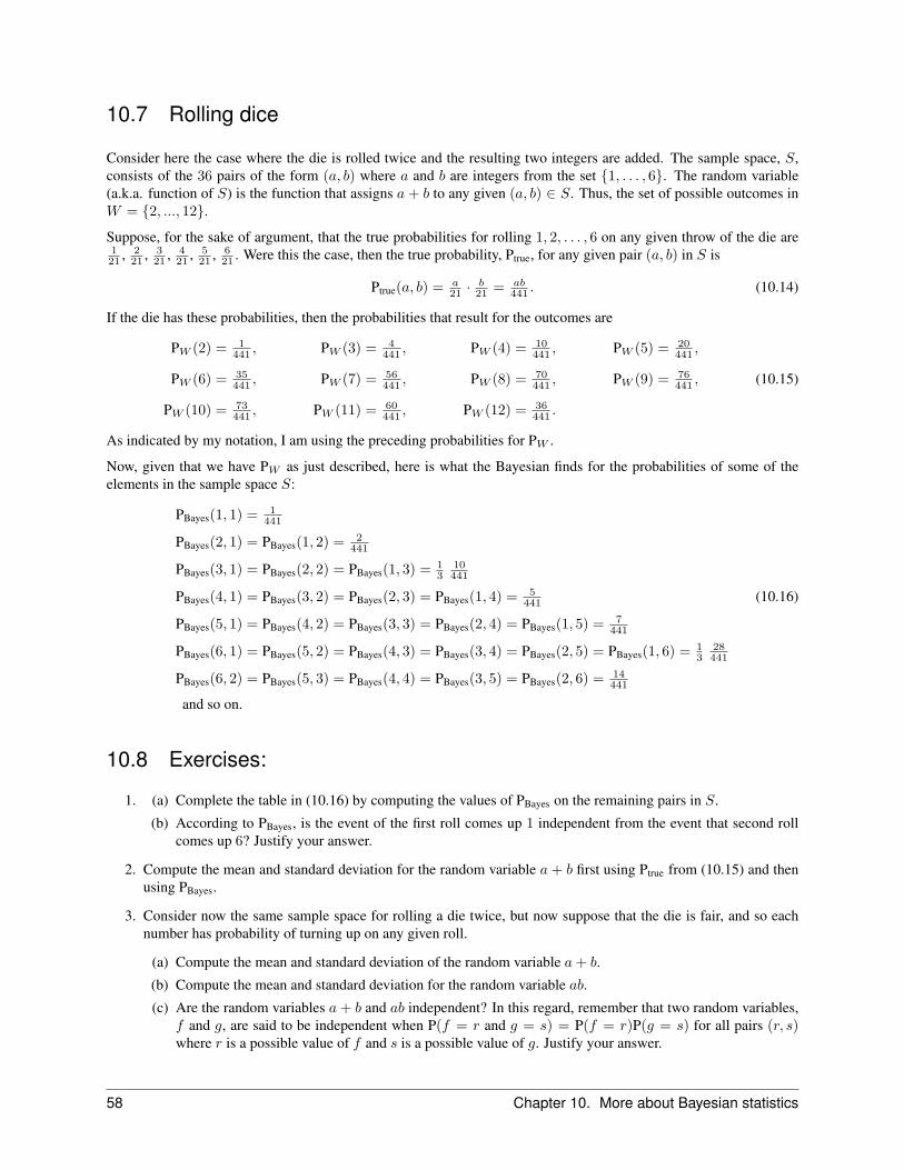
10.7 Rolling dice

Consider here the case where the die is rolled twice and the resulting two integers are added. The sample space, S,consists of the 36 pairs of the form (a, b) where a and b are integers from the set {1, . . . , 6}. The random variable(a.k.a. function of S) is the function that assigns a + b to any given (a, b) ∈ S. Thus, the set of possible outcomes inW = {2, ..., 12}.

Suppose, for the sake of argument, that the true probabilities for rolling 1, 2, . . . , 6 on any given throw of the die are121 , 2

21 , 321 , 4

21 , 521 , 6

21 . Were this the case, then the true probability, Ptrue, for any given pair (a, b) in S is

Ptrue(a, b) = a21 ·

b21 = ab

441 . (10.14)

If the die has these probabilities, then the probabilities that result for the outcomes are

PW (2) = 1441 , PW (3) = 4

441 , PW (4) = 10441 , PW (5) = 20

441 ,

PW (6) = 35441 , PW (7) = 56

441 , PW (8) = 70441 , PW (9) = 76

441 , (10.15)

PW (10) = 73441 , PW (11) = 60

441 , PW (12) = 36441 .

As indicated by my notation, I am using the preceding probabilities for PW .

Now, given that we have PW as just described, here is what the Bayesian finds for the probabilities of some of theelements in the sample space S:

PBayes(1, 1) = 1441

PBayes(2, 1) = PBayes(1, 2) = 2441

PBayes(3, 1) = PBayes(2, 2) = PBayes(1, 3) = 13

10441

PBayes(4, 1) = PBayes(3, 2) = PBayes(2, 3) = PBayes(1, 4) = 5441 (10.16)

PBayes(5, 1) = PBayes(4, 2) = PBayes(3, 3) = PBayes(2, 4) = PBayes(1, 5) = 7441

PBayes(6, 1) = PBayes(5, 2) = PBayes(4, 3) = PBayes(3, 4) = PBayes(2, 5) = PBayes(1, 6) = 13

28441

PBayes(6, 2) = PBayes(5, 3) = PBayes(4, 4) = PBayes(3, 5) = PBayes(2, 6) = 14441

and so on.

10.8 Exercises:

1. (a) Complete the table in (10.16) by computing the values of PBayes on the remaining pairs in S.

(b) According to PBayes, is the event of the first roll comes up 1 independent from the event that second rollcomes up 6? Justify your answer.

2. Compute the mean and standard deviation for the random variable a + b first using Ptrue from (10.15) and thenusing PBayes.

3. Consider now the same sample space for rolling a die twice, but now suppose that the die is fair, and so eachnumber has probability of turning up on any given roll.

(a) Compute the mean and standard deviation of the random variable a+ b.

(b) Compute the mean and standard deviation for the random variable ab.

(c) Are the random variables a+ b and ab independent? In this regard, remember that two random variables,f and g, are said to be independent when P(f = r and g = s) = P(f = r)P(g = s) for all pairs (r, s)where r is a possible value of f and s is a possible value of g. Justify your answer.

58 Chapter 10. More about Bayesian statistics

CHAPTER

ELEVEN

Common probability functions

There are certain probability functions that serve as models that are commonly used when trying to decide if a givenphenomena is ‘unexpected’ or not. This chapter describes those that arise most often.

11.1 What does ‘random’ really mean?

Consider a bacterial cell that moves one cell length, either to the right or left, in each unit of time. If we start somelarge number of these cells at x = 0 and wait t units of time, we can determine a function, pt(x), which is the fractionof bacteria that end up at position x ∈ {0,±1,±2, . . .} at time t. We can now ask: What do we expect the functionx→ pt(x) to look like?

Suppose that we think that the bacteria is moving ‘randomly’. Two questions then arise:

• How do we translate our intuitive notion of the English term ‘random’ into a predic-tion for pt(x)?

• Granted we have a prediction, for each t and x, then how far must pt(x) be fromits predicted value before we must accept the fact that the bacteria is not movingaccording to our preconceived notion of random?

(11.1)

These questions go straight to the heart of what is called the ‘scientific method’. We made a hypothesis: The bacteriummoves left or right at random’. We want to first generate some testable predictions of the hypothesis (the first pointin (11.1)), and then compare these predictions with experiment. The second point in (11.1) asks for criterion to use toevaluate whether the experiment confirms or rejects our hypothesis.

The first question in (11.1) is the provenance of ‘probability theory’ and the second the provenance of ‘statistics’. Thischapter addresses the first question in (11.1), while aspects of the second are addressed in some of the subsequentchapters.

11.2 A mathematical translation of the term ‘random’

To say that an element is chosen from a given set at ‘random’ is traditionally given the following mathematical defini-tion:

Probabilities are defined using the probability function that assigns all elements the sameprobability. If the set has L elements, then the probability of any given element appearingis 1L .

(11.2)

The probability function that assigns this constant value to all elements is called the uniform probability function.

59

Here is an archetypal example: A coin is flipped N times. Our sample space is the set S that consists of the 2N possiblesequences (±1,±1, . . . ,±1), where +1 is in the kth spot when the kth flip landed heads up, while −1 sits in this slotwhen the kth flip landed tails up. If I assume that the appearance of heads on any flip has probability , and that theappearance of heads on any subset of flips has no bearing on what happens in the other flips, then I would predictthat the frequencies of appearance of any given sequence in S is 2−N . This is to say that I would use the uniformprobability function on S to predict the frequency of appearance of any subset of its elements.

Note that after setting N = t, this same sample space describes all of the possibilities for the moves of our bacteriumfrom Section 11.1, above.

Here is another example: You go to a casino to watch people playing the game of ‘craps’. Remember that this game isplayed by rolling two six-sided dice, and looking at the numbers that show on the top faces when the dice stop rolling.The sample space for one play of the game is the set of 36 elements where each is of the form (a, b) for a, b integersfrom 1 through 6. If I believe that the dice are ‘fair’ and that the appearance of any given number on one die has nobearing on what appears on the other, then I would use the uniform probability function on S to predict the frequencyof appearance of any given outcome.

I might watch N games of craps played. In this case, the sample space is the set of 36N possible sequence of the form((a1, b1), . . . , (aN , bN )) where each ak and each bk is a number from 1 through 6. If I believe that the appearance ofany face on the dice is as likely as any other, and if I believe that the appearance of any sequence in any given subset ofthe N games has no affect on what happens in the other games, then I would make my predictions for the frequenciesusing the uniform probability function on this 36N element sample space.

What follows is yet one more example: Look at a single stranded DNA molecule that is composed of N bases strungend to end. As each cite on the DNA molecule can be occupied by one of 4 bases, the sample space that describes thevarious possibilities for this DNA molecule is the 4N element set whose typical member is a sequence (θ1, . . . , θN )where each θk is either A, C, G or T. If I believe that each such letter is equally likely to appear, and that the appearanceof a given letter in any one slot has no bearing on what happens in the other slots, then I would use the uniformprobability function to predict the frequencies of occurrences of the various letters in length N strand of DNA.

You might think that the uniform probability distribution is frightfully dull – after all, how much can you say about aconstant?

11.3 Some standard counting solutions

The uniform probability distribution becomes interesting when you consider the probabilities for certain subsets,or the probabilities for the values of certain random variables. To motivate our interest in the uniform probabilitydistribution, consider first its appearance in the case of bacteria. Here, our model of random behavior takes S as justdescribed, the set of 2N sequences of the form (α1, α2, . . . , αN ), where each αk is 1 or −1. Now define f so thatf(α1, · · · , αN ) = α1 + α2 + · · · + αN and ask for the probabilities of the possible values of f . With regards tobacteria, f tells us the position of the bacteria after N steps in the model where the bacteria moves right or left withequal probability at each step. The probabilities for the possible values of f provide the theoretical predictions for themeasured function pt(x) in the case that t = N . Thus, uniform probability function on S predicts that pt=N (x) isequal to 2−N times the number of sequences in S whose entries add up to x.

Note that pN (x) is not the uniform probability function on the set of possible values for f . To see that such is thecase, note that the possible values for x are the integers from the set W = {−N,−N + 2, . . . , N − 2, N}. This sethas N + 1 elements. Since only the sequence (−1,−1, . . . ,−1) has entries that sum to −N , so pN (−N) = 2−N .Meanwhile, the only sequence from S whose entries sum to N is (1, 1, . . . , 1), and so pN (N) = 2−N also. Howeverthere areN elements in S whose entries sum to−N+2, these the elements that have a single entry equal to +1. Thus,pN (−N + 2) = N2−N . A similar count finds pN (N − 2) = N2−N .

In general, if a set S has N elements and a subset K ⊂ S has k elements, then the uniform probability distribution onS gives probability k

N to the set K. Even so, it may be some task to count the elements in any given set. Moreover,the degree of difficulty may depend on the manner in which the set is described. There are, however, some standardcounting formulae available to facilitate things. For example, let S denote the sample space with 2N elements as

60 Chapter 11. Common probability functions

described above. For n ∈ {0, 1, . . . , N}, let Kn denote the subset of elements in S with n occurrences of +1, thuswith N − n occurrences of −1. Note that Kn has an alternate description, this as the set of elements on whichf(α1, . . . , αN ) = α1 + α2 + · · · + αN has value −N + 2n. Thus, the number of elements in Kn times 2−N givespt=N (x) in the case where x = −N + 2n.

In any event, here is a basic fact:

The set Kn hasN !

n!(N − n)!members. (11.3)

In this regard, remember that k! is defined for any positive integer k as k(k− 1)(k− 2) · · · 1. Also, 0! is defined to byequal to 1. For those who don’t like to take facts without proof, I explain in the last section below how to derive (11.3)and also the formulae that follow.

By the way, arises often enough in counting problems to warrant its own symbol, this(N

n

). (11.4)

Here is another standard counting formula: Let b ≥ 1 be given, and let S denote the set of bN elements of the form(β1, . . . , βN ), where each βk is now {1, . . . , b}. For example, if b = 6, then S is the sample space for the list of facesthat appear when a six-sided die is rolled N times. If b = 4, then S is the sample space for the possible single strandsof DNA with N bases.

If N > b, then each element in S has at least one βk that is the same as another. If N ≤ b, then there can be elementsin S where no two βk are the same. Fix b and let Eb denote the subset of those N -tuples (β1, . . . , βN ) where no twoβk are identical.

The set Eb hasb!

(b−N)!members. (11.5)

The case n = N in (11.5) provides the following:

There are N ! ways to order a set of N distinct elements. (11.6)

Here, a set of elements is ‘ordered’ simply by listing them one after the other. For example, the set that consistsof 1 apple and 1 orange has two orderings, (apple, orange) and (orange, apple). The set that consist of the threeelements {apple, orange, grape} has six orderings, (apple, orange, grape), (apple, grape, orange), (orange, grape,apple), (orange, apple, grape), (grape, apple, orange), (grape, orange, apple).

Here is a direct argument for (11.6): To count the number of orderings, note that there are N possible choices for thefirst in line. With the first in line chosen, then N − 1 elements can be second in line. With the first two in line chosen,there are N − 2 left that can be third in line. Continuing in this reasoning leads to (11.6).

11.4 Some standard probability functions

The counting formulae just presented can be used to derive some probability functions that you will almost surely seeagain and again in your scientific career.

The Equal Probability Binomial: Let S denote the sample space with the 2N elements of the form (α1, . . . , αN )where each αk can be 1 or −1. For any given integer n ∈ {0, 1, . . . , n}, let Kn denote the event that there areprecisely n occurrences of +1 in the N -tuple (α1, . . . , αN ). Then the uniform probability function on S assigns Kn

the probability

P(n) = 2−NN !

n! (N − n)!(11.7)

11.4. Some standard probability functions 61

The fact that Kn has probability P(n) follows from (11.3).

The assignment of P(n) to an integer n defines a probability function on the N + 1 element set {0, 1, . . . , N}. Thisis a probability function that is not uniform. We will investigate some of its properties below.

Equation (11.7) can be used to answer the first question in (11.1) with regards to our random bacteria in Section 11.1.To see how this comes about, let S denotes the sample space with the 2N elements of the form (±1,±1, . . . ,±1).Let f again denote the random variable that assigns α1 + · · · + αN to any given (α1, . . . , αN ). Then, the eventf = −N + 2n is exactly our set Kn. This understood, if x ∈ {−N,−N + 2, . . . , N − 2, N} then

P(the event that f = x) = 2−NN !(

N+x2

)!(N−x

2

)!. (11.8)

If we believe that the bacteria chooses left and right with equal probability, and that moves made in any subset ofthe N steps have no bearing on those made in the remaining steps, then we should be comparing our experimentallydetermined pt(x) with the N = t version of (11.8).

The Binomial Probability Function: The probability function P in (11.7) is an example of what is called thebinomial probability function on the set {0, . . . , N}. The ‘generic’ version of the binomial probability distributionrequires the choice of a number, q ∈ [0, 1]. With q chosen, the probability q-version assigns the following probabilityto an integer n:

Pq(n) = qn(1− q)N−n. (11.9)

The probability function in (11.9) arises from the sample space S whose elements are the N -tuples with elements(±1, . . . ,±1). In this regard, (11.9) arises in the case that the probability of seeing +1 in any given entry is q andthat of −1 in a given entry is 1 − q. Here, this probability function assumes that the occurrences of ±1 in any subsetof entries must have no bearing on the appearances of ±1 in the remaining entries. The probability function in (11.9)describes the probability in this case for the set Kn ⊂ S of elements with n occurrences of +1 and N −n occurrencesof −1.

One can also view the probability function in (11.9) as follows: Define a random variable, g, on S, that assigns to anygiven element the number of appearances of +1. Give S the probability function just described. Then (11.9) gives theprobability that g = n. To see why this probability is (11.9), note that the event that g = n is just our set Kn. Withthis new probability, each element in Kn has probability qn(1 − q)N−n. As (11.3) gives the number of elements inKn, its probability is therefore given by (11.9).

The probability function in (11.9) is relevant to our bacterial walking scenario when we make the hypothesis that thebacteria moves to the right at any given step with probability q, thus to the left with probability 1− q. I’ll elaborate onthis in a subsequent chapter.

Here is another example: Suppose you role a six sided die N times. I now ask fix an integer n from the set{0, 1, . . . , N} and ask for the probability that precisely n ≤ N of the rolls are such that the number 6 appears. IfI assume that the die is fair, and that the numbers that appear on any subset of rolls have no bearing on the numbersthat appear in the remaining rolls, then the probability of n occurrences of 6 in N rolls of the die is given by the q = 1

6version of (11.9). Here is why: I make an N element sequence (α1, . . . , αN ) with each αk = 1 or −1 by settingαk = +1 when 6 appears on the kth roll of the die, and setting αk = −1 when 1, 2, 3, 4, or 5 appears on the kth rollof the die. The possible sequence of this form make a 2N element set that I call S. As the probability is 1

6 for anygiven αk to equal to +1, so a given sequence from S with precisely n occurrences of +1 has probability ( 1

6 )n( 56 )N−n.

Meanwhile, the number of elements in S with n occurrences of +1 is given by (11.3). This understood, the probabilityof an element in S having n occurrences of +1 is equal to the product of (11.3) with ( 1

6 )n( 56 )N−n, and this is just the

q = 16 version of (11.9).

To give an example, consider rolling a standard, six-sided die. If the die is rolled once, the sample space consists of thenumbers {1, 2, 3, 4, 5, 6}. If the die is ‘fair’, then I would want to use the probability function that assigns the versionof (11.9).

Here is a final example: Consider a single stranded DNA molecule made of N bases. Suppose that the probabilitythat the base C appears in any given position is given by some q ∈ [0, 1]. If each base is equally likely, then q = 1

4 to


each element. If the bases that appear in any given subset of the N stranded molecule have no bearing on those thatappear in the remaining positions, then the probability that n of the N bases are C should be given by the expressionin (11.9). Note that this is a definite prediction about the DNA molecules in a given cell, and can be tested in principleby determining the percent of DNA that has the base C (cytosine). If this percentage differs significantly from 1

4 , thenat least one of our assumptions is incorrect: Either it is not true that the appearance of C in any given position hasprobability 1

4 , or it is not true that the bases that appear in a given subset of the molecule have no bearing on those thatappear in the remainder of the molecule.

I talk later about the meaning of the term ‘differs significantly from’.

The Poisson Probability Function: This is a probability function on the sample space, N = {0, 1, . . .}, the non-negative integers. As you can see, this sample space has an infinite number of elements. Even so, I define a probabilityfunction on N to be a function, P, with P(n) ∈ (0, 1) for each n, and such that∑

n=0,1,...

P(n) = P(0) + P(1) + P(2) + · · · (11.10)

is a convergent series with limit equal to 1.

As with the binomial probability function, there is a whole family of Poisson functions, one for each choice of apositive real number. Let τ > 0 denote the given choice. The τ version of the Poisson function assigns to any givennon-negative integer the probability

Pτ (n) =1n!τne−τ . (11.11)

You can see that∑

n=0,1,...Pτ (n) = 1 if you know about power series expansions of the exponential function. In

particular, the function τ → eτ has the power series expansion

eτ = 1 + τ +12τ2 +

16τ3 + · · ·+ 1

n!τn + · · · . (11.12)

Granted (11.12), then∑

n=0,1,...

1n!τ

ne−τ =

( ∑n=0,1,...

1n!τ

n

)e−τ = eτe−τ = 1.

The Poisson probability enters when trying to decide if an observed cluster of occurrences of a particular phenomenonis or is not due to chance. For example, suppose that on average, some number, ∆, of newborns in the United Statescarry a certain birth defect. Suppose that some number, n, of such births are observed in 2006. Does this constitute anunexpected clustering that should be investigated? If the defects are unrelated and if the causative agent is similar inall cases over the years, then the probability of n occurrences in a given year should be very close to the value of theτ = ∆ version of the Poisson function Pτ (n).

Here is another example from epidemiology: Suppose that the university health service sees an average of 10 casesof pneumonia each winter. Granted that the conditions that prevail this coming winter are no different than thosein the past, and granted that cases of pneumonia are unrelated, what is the probability of there being 20 cases ofpneumonia this winter? If these assumptions are valid, then the τ = 10 Poisson function should be used to computethis probability. In particular, P10(20) ≈ 0.0058.

What follows is a final example, this related to discerning whether patterns are ‘random’ or not. Consider, for example,the sightings of ‘sea monsters’. In particular, you want to know if more sea monster sightings have occurred in theBermuda Triangle then can be accounted for by chance. One way to proceed is to catalogue all such sightings tocompute the average number of sightings per day per ship. Let us denote this average by δ. Now, estimate the numberof ‘ship days’ that are accounted for by ships while in the Bermuda Triangle. Let N denote this last number. Ifsightings of sea monsters are unrelated and if any two ships on any two days in any two parts of the ocean are equallylikely to sight a sea monster, then the probability of n sightings in the Bermuda triangle is given by the τ = Nδ versionof (11.11).

I give some further examples of how the Poisson function is used in a separate chapter.

11.4. Some standard probability functions 63

By the way, the Poisson function is an N → ∞ limit of the binomial function. To be more precise, the τ version ofthe Poisson probability Pτ (n) is the N → ∞ limit of the versions of (11.9) with q set equal to 1 − e−τ/N . This is tosay that

1n!τne−τ = limN→∞

N !n! (N − n)!

(1− e−τ/N

)ne(−τ/N)(N−n). (11.13)

The proof that (11.13) holds takes us in directions that we don’t have time for here. Let me just say that it uses theapproximation to the factorial known as Stirling’s formula:

n! =√

2πne−nnn (1 + error) (11.14)

where the term designated as ‘error’ limits to zero as n → ∞. For example, the ratio with n! the numerator and√2πne−nnn as the denominator is as follows for various choices of n:

n n!√2πne−nnn

2 7.75 1.01610 1.00820 1.004100 1.0008

Thus, the approximation in (11.14) serves for most uses.

11.5 Means and standard deviations

Let me remind you that if P is a probability function on some subset S of the set of integers, then its mean, µ, is definedto be

µ =∑n∈S

nP(n) (11.15)

and the square of its standard deviation, σ, is defined to be

σ2 =∑n∈S

(n− µ)2P(n). (11.16)

Here, one should keep in mind that when S is an infinite number of elements, then µ and σ are defined only when thecorresponding sums on the right sides of (11.15) and (11.16) are those of convergent series. The mean and standarddeviation characterize any given probability function to some extent. More to the point, both the mean and standarddeviation are often used in applications of probability and statistics.

The mean and standard deviation for the binomial probability on {0, 1, . . . , N} are

µ = Nq and σ2 = Nq(1− q). (11.17)

For the Poisson probability function on {0, 1, . . . }, they are

µ = τ and σ2 = τ. (11.18)

I describe a slick method for computing the relevant sums below.

To get more of a feel for the binomial probability function, note first that the mean for the q = 12 . version is N

2 .This conforms to the expectation that half of the entries in the ‘average’ N -tuple (α1, . . . , αN ) should be +1 and halfshould be −1. Meanwhile in the general version, the assertion that the mean is Nq suggests that the fraction q of theentries in the ‘average’ N -tuple should be +1 and the fraction (1− q) should be −1.

By the way, one can ask for the value of n that makes Pq(n) largest. To see what this is, note that

Pq(n+ 1)Pq(n)

=N − nn+ 1

q

1− q. (11.19)


This ratio is less than 1 if and only ifn < Nq − (1− q). (11.20)

Since (1− q) < 1, this then means that the ratio in (11.19) peaks at a value of n that is within ±1 of the mean.

In the case of the Poisson probability, the ratio Pτ (n+1)Pτ (n) is 1

n+1τ . If τ < 1, then 0 has the greatest probability ofoccurring. If τ ≥ 1, then Pτ (n) is greatest when n is the closest integer to τ − 1. Thus, the mean in this case is alsovery nearly the integer with the greatest probability of occurring.

11.6 The Chebychev theorem

As I remarked in Chapter 5, the standard deviation indicates the extent to which the probabilities concentrate aboutthe mean. To see this, consider the following remarkable fact:

The Chebychev Theorem. Suppose that P is a given probability function on a subset of the integers,{. . . ,−1, 0, 1, . . .}, one with a well defined mean µ and standard deviation σ. For any R ≥ 1, the probability as-signed to the set where |n− µ| > Rσ is less than R−2.

For example, this says that the probability of being 2σ away from the mean is less than 14 , and the probability of being

3σ away is less than 19 .

This theorem justifies the focus in the literature on the mean and standard deviation, since knowing these two numbersgives you rigorous bounds for probabilities without knowing anything else about the probability function!!

If you remember only one thing from these lecture notes, remember the Chebychev Theorem.

Here is the proof of the Chebychev theorem: Let S denote the sample space under consideration, and letE ⊂ S denotethe set where |n − µ| > Rσ. The probability of E is then

∑n∈E

P(n)). However, since |n − µ| > Rσ for n ∈ E, one

has

1 ≤ |n− µ|2

R2σ2(11.21)

on E. Thus, ∑n∈E

P(n) ≤∑n∈E

|n− µ|2

R2σ2P(n). (11.22)

To finish the story, note that the right side of (11.22) is even larger when we allow the sum to include all points in Sinstead of restricting only to points in E. Thus, we learn that∑

n∈EP(n) ≤

∑n

|n− µ|2

R2σ2P(n). (11.23)

The definition of σ2 from (11.16) can now be invoked to identify the sum on the right hand side of (11.23) with R−2.

Here is an example of how one might apply the Chebychev Theorem: I watch a six-sided die rolled 100 times and seethe number 6 appear thirty times. I wonder how likely it is to see thirty or more appearances of the number 6 giventhat the die is fair. Under the assumption that the die is fair and that the faces that appear in any given subset of the100 rolls have no bearing on those that appear in the remaining rolls, I can compute this probability using the q = 1

6version of the N = 100 binomial probability function by computing the sum P1/6(30) +P1/6(31) + · · ·+P1/6(100).Alternately, I can get an upper bound for this probability by using the Chebychev Theorem. In this regard, I note thatthe mean of the q = 1

6 and N = 100 binomial probability function is 1006 = 50

3 = 16 23 and the standard deviation

is 53

√5 ≈ 3.73. Now, 30 is 13 1

3 from the mean, and this is ≈ 3.58 standard deviations. Thus, the probability ofseeing thirty or more appearances of the number 6 in 100 rolls is no greater than (3.58)−2 ≈ 0.08. As it turns out, theprobability of seeing 6 appear thirty or more times is a good deal smaller than this.

11.6. The Chebychev theorem 65

It is usually the case that the upper bound given by the Chebychev Theorem is much greater than the true probability.Even so, the Chebychev Theorem is one of the most important things to remember from this course since it allowsyou to compute some upper bound with very little detailed knowledge of the probability function. Just two numbers,the mean and standard deviation, give you an upper bound for probabilities.

11.7 Characteristic functions

The slick computation of the mean and standard deviation that I mentioned involves the introduction of the notionof the characteristic function. The latter is a bona fide function on the real numbers that is determined by a givenprobability function on any sample space that is a subset of the non-negative integers, {0, 1, . . .}. This characteristicfunction encodes all of the probability function. Note, however, that this function is useful for practical purposes onlyto the extent that it isn’t some complicated mess.

Before turning to the definition in abstract, consider the special case where the subset is {0, 1, 2, . . . , N} and theprobability function is the q binomial function from (11.9). In this case, the characteristic function is the function of xgiven by

P(x) = (qx+ (1− q))N . (11.24)

Here is the connection between P(x) and the binomial probability function: Expand the product so as to write P asa polynomial of degree N in x. As I argue below, you will find that

P(x) = Pq(0) + xPq(1) + x2Pq(2) + · · ·+ xNPq(N). (11.25)

Thus, the coefficient of xn of this polynomial representation of P gives us the probabilities that Pq assigns to theinteger n.

To see why (11.25) is the same as (11.24), consider multiplying out an N -fold product of the form:

(a1x+ b1)(a2x+ b2) · · · (aNx+ bN ) (11.26)

A given term in the resulting sum can be labeled as (α1, . . . , αN ) where αk = 1 if the kth factor in (11.26) contributedakx, while αk = −1 if the kth factor contributes bk. The power of x for such a term is equal to the number of αkthat are +1. This is N !

n! (N−n)! , the number of elements in the set Kn that appears in (11.3). Thus, N !n! (N−n)! terms

contribute to the coefficient of xn in (11.26). In the case of (11.25), all versions of ak are equal to q, and all versionsof bk are equal to (1− q), so each term that contributes to xn is qn(1− q)N−nxn. As there are N !

n! (N−n)! of them, thecoefficient of xn in (11.24) is Pq(n) as (11.24) claims.

In general the characteristic function for a probability function, P, on a subset of {0, 1, . . .} is the polynomial or infinitepower series in x for which the coefficient of xn is P(n). This is to say that

P(x) = P(0) + P(1)x+ P(2)x2 + · · · =∑

n=0,1,2,...

P(n)xn. (11.27)

This way of coding the probability function P is practical only to the extent that the series in (11.27) sums to a relativelysimple function. I gave the q-binomial example above. In the case of the uniform probability function on {0, . . . , N},the sum in (11.27) is the function 1

N+11−xN+1

1−x . I argue momentarily that the τ version of the Poisson probabilityfunction on {0, 1, 2, . . . } gives

P(x) = e(x−1)τ . (11.28)

In general, there are two salient features of a characteristic polynomial: First, the values of P , its derivative, and its


second derivative at x = 1 are:

• P(1) = 1

•(d

dxP

)∣∣∣∣x=1

= µ

•(d2

dx2P

)∣∣∣∣x=1

= σ2 + µ(µ− 1)

(11.29)

Second, the values of the value of P , its derivative and its higher order derivatives at x = 0 determine P since

1n!

(dn

dxnP

)∣∣∣∣x=0

= P(n). (11.30)

This is how the function x → P(x) encodes all of the information that can be obtained from the given probabilityfunction P.

To explain how (11.29) follows from the definition in (11.27), note first that P(1) = P(0)+P(1)+· · · , and this is equalto 1 since the sum of the probabilities must be 1. Meanwhile, the derivative of P at x = 1 is 1 · P(1) + 2 · P(2) + · · · ,and this is sum is the definition of the mean µ. With the help of (11.16), a very similar argument establishes the thirdpoint in (11.29).

I can use (11.29) to get my slick calculations of the mean and standard deviations for the binomial probability function.In this case, P is given in (11.24) and so

d

dxP = Nq (qx+ (1− q))N−1

. (11.31)

Set x = 1 here to find the mean equal to Nq as claimed. Meanwhile

d2

dx2P = N(N − 1)q2 (qx+ (1− q))N−1

, (11.32)

Set x = 1 here finds the right-hand side of (11.32) equal to N(N − 1)q2. Granted this and the fact that µ = qN , thenthe third point in (11.29) find σ2 equal to

N(N − 1)q2 −N2q2 +Nq = Nq(1− q), (11.33)

which is the asserted value.

For the Poisson probability function, the characteristic polynomial is the infinite power series

Pτ (0) + xPτ (1) + x2Pτ (2) + · · · =(

1 + xτ +12x2τ2 +

16x3τ3 + · · ·+ 1

n!xnτn + · · ·

)e−τ . (11.34)

As can be seen by replacing τ in (11.12) with xτ , the sum on the right here is exτ . Thus, P(x) = e(x−1)τ as claimedby (11.28). Note that the first and second derivatives of this function at x = 1 are both equal to τ . With (11.29), thislast fact serves to justify the claim that the both the mean and standard deviation for the Poisson probability are equalto τ .

The characteristic polynomial for a probability function is used to simplify seemingly hard computations in the mannerjust illustrated in the cases where the defining sum in (11.27) can be identified with the power series expansion of awell known function. The characteristic function has no practical use when the power series expansion is not that of asimple function.

11.8 Loose ends about counting elements in various sets

My purpose in this last section is to explain where the formula in (11.3) and (11.5) come from. To start, consider (11.5).There are b choices for β1. With β1 chosen, there are b − 1 choices for β2, one less than that for β1 since we are not

11.8. Loose ends about counting elements in various sets 67

allowed to have these two equal. Given choices for β1 and β2, there are b − 2 choices for β3. Continuing in thisvein finds b − k choices available for βk+1 if (β1, . . . , βk) have been chosen. Thus, the total number of choices isb(b− 1) · · · (b−N + 1), and this is the claim in (11.5).

To see how (11.3) arises, let me introduce the following notation: Let mn(N) denote the number of elements in the(α1, . . . , αN ) version of Kn. If we are counting elements in this set, then we can divide this version of Kn into twosubsets, one where α1 = 1 and the other where α1 = −1. The number of elements in the first is mn−1(N − 1) sincethe (N − 1)-tuple (α2, . . . , αN ) must have n− 1 occurrences of +1. The number in the second is mn(N − 1) sincein this case, the (N − 1)-tuple (α2, . . . , αN ) must have all of the n occurrences of +1. Thus, we see that

mn(N) = mn−1(N − 1) +mn(N − 1). (11.35)

I will now make this last formula look like a matrix equation. For this purpose, fix some integer T ≥ 1 and make aT -component vector, ~m(N), whose coefficients are the values of mn for the cases that 1 ≤ n ≤ T . This equationasserts that ~m(N) = A~m(N − 1) where A is the matrix with Ak,k and Ak,k−1 both equal to 1 and all other entriesequal to zero. Iterating the equation ~m(N) = A~m(N − 1) finds

~m(N) = AN−1 ~m(1), (11.36)

where ~m(1) is the vector with top component 1 and all others equal to zero.

Now, we don’t have the machinery to realistically compute AN−1, so instead, lets just verify that the expressionin (11.3) gives the solution to (11.35). In this regard, note that ~m(N) is completely determined from ~m(1) us-ing (11.36), and so if we believe that we have a set {~m(1), ~m(2), . . . } of solutions, then we need only plug in ourcandidate and see if (11.36) holds. This is to say that in order to verify that (11.3) is the correct, one need only checkthat the formula in (11.36) holds. This amounts to verifying that

N !n! (N − n)!

=(N − 1)!

(n− 1)! (N − n)!+

(N − 1)!n! (N − n− 1)!

. (11.37)

I leave this task to you.

11.9 A Nobel Prize for the clever use of statistics

The 1969 Nobel Prize for Physiology and Medicine was given to Max Delbruck and Salvador Luria for work that hada crucial statistical component. What follows is a rough description of their Nobel Prize winning work.

Prior to Delbruck and Luria’s Nobel Prize winning work1 in 1943, there were two popular explanations for the evo-lution of new traits in bacteria. Here is the first: Random mutations occur as reproduction proceeds in a population.Therefore, no population of size greater than 1 is completely homogeneous. As time goes on, environmental stressesfavor certain variations over others, and so certain pre-existing variants will come to dominate any given population.This view of evolution is essentially that proposed by Darwin. There is, in contrast, the so called Lamarckian pro-posal: Environmental stresses cause new traits to arise amongst some individuals in any given population, and theseare subsequently favored. What follows summarizes these two proposals:

Darwin: Evolution occurs through the selection due to environmen-tal stresses of the most favorable traits from a suite of pre-existing traits.

Lamarck: Evolution occurs when environmental stresses force new,more favorable traits to arise.

Max Delbruck and Salvador Luria shared the 1969 Nobel Prize in Physiology and Medicine for an experiment, donein 1943, that distinguished between these two proposals as explanations for the evolution of immunity in bacterium.The results conclusively favored Darwin over Lamarck.

1Luria, SE, Delbruck, M., “Mutations of Bacteria from Virus Sensitivity to Virus Resistance” Genetics 28 (1943) 491-511.


What follows is an idealized version of what Luria and Delbruck did. They were working with a species of bacteriathat was susceptible to a mostly lethal virus. (A virus that attacks bacteria is called a ‘phage’.) They started a largenumber of colonies, each with one of these bacteria, and fed these colonies well for some length of time T . Here,it is convenient to measure time in units so that a change of one unit of time is the mean time between successivegenerations. With these units understood, each colony contained roughlyN = 2T bacteria. Each of their colonies wasthen exposed to the virus. Shortly after exposure to the virus, the number of members in each colony were counted.I use K to denote the number of colonies. The count of the number of living bacteria in each colony after phageinfection gives a list of numbers that I write as (z1, z2, . . . , zK). This set of numbers constitutes the experimental data.With regards to this list, it is sufficient for this simplified version of the story to focus only on

µexp =1K

∑1≤j≤K

zj and σ2exp =

1K

∑1≤j≤K

(zj − µexp)2. (11.38)

Luria and Delbruck realized that µexp and σ2exp can distinguish between the Darwin and Lamarck proposals. To explain

their thinking, consider first what one would expect were the Lamarck proposal true. Let p denote the probabilitythat exposure to the virus causes a mutation in any given bacterium that allows the bacterium to survive the infection.The probability of n surviving bacteria in a colony with N members should be given by the binomial probabilityfunction from (11.9) as defined using p andN in lieu of q and N . Thus, this probability is N !

n! (N−n)!pn(1−p)N−n. In

particular, the mean number of survivors should be pN and the square of the standard deviation should be p(1− p)N .This is to say that the Lamarck proposal predicts that the experimental data

µexp ≈ pN and σ2exp ≈ p(1− p)N. (11.39)

Not knowing the value for p, one can none the less say that the Lamarck proposal predicts the following:

σ2exp

µexp≈ 1− p. (11.40)

Note in particular that this number is independent of N and K; and in any event it is very close to 1 when p is small.Small p is expected.

Now consider the Darwinian proposal: In this case, there is some small, but non-zero probability, I’ll call it p, forthe founding bacterium of any given colony to have a mutation that renders it immune to the virus. If the founderof a colony has this mutation, then it is unaffected by the virus as are all of its descendents. So, a colony with animmune founder should have population 2T = N after viral attack. If a colony is founded by a bacterium without thismutation, then its population after the viral attack should be very small. Thus, in this ideal situation, the Darwinianproposal predicts that each zj should be either nearly zero or nearly N .

If K colonies are started, then the probability that n of them are founded by an immune bacterium is given by thebinomial probability function from (11.9) as defined now using p and K in lieu of q and N . Thus, this probability isK

n! (K−n)!pn(1− p)K−n. Note that the mean of this is pK and the square of the standard deviation is p(1− p)K. As a

consequence, the Darwin proposal predicts that µexp and σ2exp should be roughly

• µexp ≈∑

0≤n≤K

(Probability of n immune founders)(K−1nN )

• σ2exp ≈

∑0≤n≤K

(Probability of n immune founders)(K−1nN 2)− µ2exp.

(11.41)

These sums give the predictions µexp ≈ pN and σ2exp ≈ p(1− p)N 2. As a consequence, the Darwin proposal predicts

the ratioσ2

exp

µexp≈ (1− p)N . (11.42)

Note in particular that if p is small, then this number is roughly N = 2T while that in (11.40) is roughly 1.

Delbruck and Luria saw statistics that conclusively favored the Darwin proposal over the Lamarck one.

11.9. A Nobel Prize for the clever use of statistics 69

11.10 Exercises:

1. Let A denote the 4× 4 version of the matrix in (11.36). Thus,

A =

1 0 0 01 1 0 00 1 1 00 0 1 1

.

(a) Present the steps of the reduced row echelon reduction of A to verify that it is invertible.

(b) Find A−1 using Fact 2.3.5 of Bretscher’s book Linear Algebra with Applications.

2. Let τ denote a fixed number in (0, 1). Now define a probability function, P, on the set {0, 1, 2, . . .} by settingP(n) = (1− τ)τn.

(a) Verify that P(0) + P(1) + · · · = 1, and thus verify that P is a probability function.(If you haven’t seen how to do this, set V (n) = 1+τ+τ2+· · ·+τn. Prove that τV (n) = V (n)−1+τn+1.Then rearrange things to write V (n)(1−τ) = (1−τn+1). Now solve for V (n) and consider what happenswhen n→∞.)

(b) Sum the series P(0) +xP(1) +x2P(2) + · · · to verify that the characteristic function is the P(x) = 1−τ1−xτ .

(c) Use the formula in (11.28) to compute the mean and standard deviation of P.

(d) In the case τ = 12 , the mean is 1 and the standard deviation is

√2. As 6 ≥ µ+3σ, the Chebychev Theorem

asserts that the probability for the set {6, 7, . . .} should be less than 19 . Verify this prediction by summing

P(6) + P(7) + · · · .(e) In the case τ = 2

3 , the mean is 2 and σ =√

6. Verify the prediction of the Chebychev Theorem that{7, 8, . . .} has probability less than 1

4 by computing the sum P(7) + P(8)) + · · · .

3. This exercise fills in some of the details in the verification of (11.3).

(a) Multiply both sides of (11.37) by (n − 1)!(N − n − 1)! and divide both sides of the result by (N − 1)!Give the resulting equation.

(b) Use this last result to verify (11.37).

4. Suppose that I have a bag with 6 red grapes and 5 green ones. I reach in with my eyes closed and pick a grapeat random. After looking at its color, I replace the grape, shake up the bag and redo this experiment, 10 timesin all. Let n be an integer between 0 and 10. Assume that any given grape is chosen at random each time, andthat my choices in any given subset of the experiments have no bearing on those of the remaining experiments.What is the probability of choosing exactly n green grapes in the 10 experiments?

5. The purpose of this exercise is to explore the q = 12 version of the binomial probability function, thus the

function P(n) that appears in (11.7).

(a) As explained in the text, P(n) is largest when n = N2 in the case that N is even. Use Stirling’s formula to

justify the claim that P(N2 ) ≈√

2πN when N is even and very large. Compare this last number with the

true value given by (11.7) for N = 10 and N = 100.

(b) Suppose that N is a positive, even integer. The mean for the q = 12 binomial probability function for the

set {0, 1, . . . , N} is µ = 12N and the standard deviation is σ = 1

2

√N . Use the Chebychev theorem in

the cases N = 36 and 64 to find an upper bound for the probability of the set of n ≤ 10. Then, use acalculator to compute this probability using the formula in (11.7).

6. The purpose of this problem is to explore the Poisson probability function in the context of discerning patterns.Suppose that I am a police captain in Boston in charge of a 10 block by 10 block neighborhood. Thus aneighborhood of 100 squares, each 1 block on a side. I note that in over the years, my force was asked torespond to an average of 500 calls from the neighborhood, thus an average of 5 per square block per year. The


police station is in the square at one corner of the neighborhood. There were no calls from this square last year.The square furthest from the police station recorded 15 calls. Under the assumption that a call is as likely tocome from any one square as any other, and that whether or not a call has come in from a square has no bearingon when the next call will come in from that square or any other square, give

(a) the probability that there are no calls from the police station’s square, and

(b) the probability that there are 15 calls from the square furthest from the police station’s square.

7. This problem is a continuation of the preceding one. The purpose here is to let you see how an event withsmall probability to occur in any one place can have a reasonably large probability of appearing somewhere. Inparticular, the goal for this exercise is to compute the probability that there is at least one square with no calls.For this purpose, let q denote your answer to Problem 6a.

(a) Explain why the probability that every square has at least one call is (1− q)100.

(b) Explain why the probability that at least one square has no calls is 1− (1− q)100.

8. This is a problem whose purpose is to get you to think about counting and probability. The point is that beingable to make an accurate count of the various ways that a given outcome can arise is crucial to making a correctcalculation of probabilities.

Here is the scenario: In baseball’s World Series, the two league champions in a given year meet to see whichteam is the best in baseball for that year. The teams play games sequentially until one or the other wins fourgames. The team that wins four games is declared the World Champion. Thus, the World Series can involveanywhere from 4 to 7 games. Since 1923, there have been 16 years where the series ended after 4 games, 16years when it ended after 5 games, 18 years when it ended after 6 games and 33 years when it ended after7 games. See http://mlb.mlb.com/NASApp/mlb/mlb/history/postseason/mlb_ws.jsp?feature=recaps_index.

Thus, the relative frequencies for 4, 5, 6 and 7 game series are:

4 games: 1683 ≈ 0.19

5 games: 1683 ≈ 0.19

6 games: 1883 ≈ 0.22

7 games: 3383 ≈ 0.40

Here is a question: What is the expected frequency of 4, 5, 6 and 7 game series if we assume that the two teamshave a 50-50 chance of winning any given game, and if we assume that the event of winning any one game isindependent of the event of winning any other. To answer this question, let A and N denote the two teams.

(a) What is the probability for A to win the first 4 games? Likewise, what is the probability for N?

(b) Explain why the probability for the World series to last 4 games is 18 = 0.125.

(c) Explain why the probability for the World Series to last 5 games is equal to

2(

43

)(12

)4(12

)=

14

= 0.25.

(d) Explain why the probability for the World Series to last 6 games is

2(

53

)(12

)5(12

)=

516

= 0.3125.

(e) Explain why the probability for the World Series to last 7 games is

2(

63

)(12

)6(12

)=

516

= 0.3125.

11.10. Exercises 71

http://mlb.mlb.com/NASApp/mlb/mlb/history/postseason/mlb_ws.jsp?feature=recaps_index

http://mlb.mlb.com/NASApp/mlb/mlb/history/postseason/mlb_ws.jsp?feature=recaps_index

CHAPTER

TWELVE

P-values

My purpose in this chapter is to describe a criterion for deciding when data is “surprising”. For example, suppose thatyou flip a coin 100 times and see 60 heads. Should you be surprised? Should you question your belief that the coin isfair? More generally, how many heads should appear before you question the coin’s fairness? These are the sorts ofquestions that I will address below.

12.1 Point statistics

Suppose that you do an experiment N times and find that a certain event occurs m times out of the N experiments.Can one determine from this data a probability function for the event to occur? For example, I flip a coin 100 timesand see 60 heads. Can I determine a probability function for heads to appear?

If we assume that the N experiments are identical in set up, and that the appearance of the event in any one hasno bearing on its appearance in any other, then we can propose the following hypothesis: The event occurs in anygiven experiment with probability q (to be determined) and so the probability that some n ≤ N events occurs in Nexperiments is given by the q-version of the binomial function, thus

Pq(n) =N !

n!(N − n)!qn(1− q)N−n. (12.1)

The question now is: What value should be used for q?

The use of experimental data to estimate a single parameter – q in this case – is an example of what are called pointstatistics. Now, it is important for you to realize that there are various ways to obtain a “reasonable” value to use forq. Here are some:

• Since we actually found m events in N trials, take the value of q that gives m for the mean of the probabilityfunction in (12.1). With reference to (11.17) in the previous chapter, this choice for q is m

N .

• Take q to so that n = m is the integer with the maximal probability. If you recall (11.19) from the previouschapter, this entails taking q so that both

Pq(m)Pq(m+ 1)

> 1 andPq(m− 1)

Pq(m)< 1. (12.2)

This then implies that mN+1 < q < m+1

N+1 . Note that q = mN satisfies these conditions.

With regards to my example of flipping a coin 100 times and seeing 60 heads appear, these arguments would lead meto postulate that the probability of seeing some number, n, of heads, is given by the q = 0.6 version of (12.1).

72

12.2 P -value and bad choices

A different approach asks for the bad choices of q rather than the “best” choice. The business of ruling out variouschoices for q is more in the spirit of the scientific method. Moreover, giving the unlikely choices for q is usuallymuch more useful to others than simply giving your favorite candidate. What follows explains how statisticians oftendetermine the likelihood that a given choice for q is realistic.

For this purpose, suppose that we have some value for q in mind. There is some general agreement that q is not areasonable choice when the following occurs:

There is small probability as computed by the q-version of (12.1) of there being the observed m occur-rences of the event of interest.

To make the notion of small probability precise, statisticians have introduced the notion of the “P -value” of a mea-surement. This is defined with respect to some hypothetical probability function, such as our q-version of (12.1). Inour case, the P -value of m is the probability for the subset of numbers n ∈ {0, 1, . . . , N} that are at least as far fromthe mean, qN , as ism. For example,m has P -value 1

2 in the case that (12.1) assigns probability 12 to the set of integers

n that obey |n −Nq| ≥ |m −Nq|. A P -value that is less than 0.05 is deemed significant by statisticians. This is tosay that if m has such a P -value, then q is deemed unlikely to be incorrect.

In general, the definition of the P-value for any measurement is along the same lines:

Definition: Suppose that a probability function on the set of possible measurements for some experiment is proposed.The P -value of any given measurement is the probability for the subset of values that lie as far or farther from themean of this probability function than the given measurement. The P -value is deemed significant if it is smaller than0.05.

Note here that this definition requires computing the probability of being both greater than the mean and less than thenthe mean. There is also the notion of a one-sided P -value. This computes the probability of being on the same side ofthe mean as the observed value, and at least as far from the mean as the observed value. Thus, if the observed value isgreater than the mean, the 1-sided P -value computes the probability that a measurement will be as large or larger thanthe observed value. If the observed value is less than the mean, then the 1-sided P -value computes the probability ofbeing as small or smaller than the observed value. There are other versions of P -value used besides that defined aboveand the 1-sided P -values. However, in these lecture notes, P -value means what is written in the preceding definition.But, keep in mind when reading the literature or other texts that there are alternate definitions.

Consider now the example where I flip a coin 100 times and find 60 heads. If I want to throw doubt on the hypothesisthat the coin is fair, I should compute the P -value of 60 using the q = 1

2 version of the binomial probability functionin (12.1). This means computing P1/2(60) + P1/2(61) + · · · + P1/2(100) + P1/2(40) + P1/2(39) + · · · + P1/2(1).The latter sum gives the probability of seeing a number of heads appear that is at least as far from the mean, 50, as is60. My calculator finds that this sum is 0.057. Thus, the P -value of 60 is greater than 0.05 and so I hesitate to rejectthe hypothesis that the coin is fair.

An upper bound for the P -value that uses only the mean and standard deviation of a probability function can be hadusing the Chebychev theorem in Chapter 11. As you should recall, this theorem asserts that the probability of findinga measurement with distance Rσ from the mean is less than R−2. Here, σ denotes the standard deviation of the givenprobability function. Granted this, a measurement that differs from the mean by 5σ or more has probability less than0.04 and so has a significant P -value. Such being the case, the 5σ bound is often used in lieu of the 0.05 bound.

To return to our binomial case, to say that m differs from the mean, Nq, by at least 5σ, is to say that

|m−Nq| ≥ 5(Nq(1− q))1/2. (12.3)

We would consider q to be a “bad” choice in the case that (12.3) holds.

In the case of my coin flip example, with N = 100 and q = 12 , the standard deviation is 5. Thus, 60 heads is only 2

standard deviations from the mean, which is less than the 5σ criterion used above.

When using the Chebychev theorem to get an upper bound for a P -value, remember the following:

12.2. P -value and bad choices 73

If an outcome differs from the mean by 5σ or more, then it’s P -value is necessarily smaller than 0.05.

The converse of this last statement is not true. An event can have P -value that is smaller than 0.05 yet differ from themean by less than 5σ. Take for example the case where I flip a coin 100 times and now see 61 heads instead of 60.Under the assumption that the coin is fair, the P -value of 61 heads is 0.0452. This is less than 0.05. However, 61 is2.2σ from the mean.

12.3 A binomial example using DNA

As you may recall, a strand of a DNA molecule consists of a chain of smaller molecules tied end to end. Each smallmolecule in the chain is one of four types, these labeled A, T, G and C. Suppose we see that G appears some n timeson some length N strand of DNA. Should this be considered unusual?

To make this question precise, we have to decide how to quantify the term unusual, and this means choosing a proba-bility function for the sample space whose elements consist of all lengthN strings of letters, where each letter is eitherA, C, G or T. For example, the assumption that the appearances of any given molecule on the DNA strand are occurringat random suggests that we take the probability of any given letter A, C, G or T appearing at any given position tobe 1

4 . Thus, the probability that G does not appear at any given location is 34 , and so the probability that there are n

appearances of G in a length N string (if our random model is correct) would be given by the q = 34 version of the

binomial function in equation (12.1).

This information by itself is not too useful. A more useful way to measure whether n appearances of G is unusual isto ask for the probability in our q = 1

4 binomial model for more (or less) appearances of G to occur. This is to saythat if we think that there are too many G’s for the appearance to be random then we should consider the probabilityas determined by our q = 1

4 binomial function of there being at least this many G’s appearing. Thus, we should becomputing the P -value of the measured number, n. In the binomial case with q = 1

4 , this means computing

∑k∈B

N !k!(N − k)!

(14

)k (34

)N−k, (12.4)

where the sum is over all integers k from the set, B, of integers in {0, . . . , N} that obey |b− N4 | ≥ |n−

N4 |.

Suppose, for instance that we have a strand of N = 20 bases and see 10 appearances of G. Does this suggest that ourhypothesis is incorrect about G’s appearance being random in the sense just defined? To answer this question, I wouldcompute the P -value of 10. This means computing the sum in (12.4) with N = 20 and B the subset in {0, . . . , 20} ofintegers b with either b = 0 or b ≥ 10. As it turns out, this sum is close to 0.017. The P -value is less than 0.05 and sowe are told to doubt the hypothesis that the G appears at random.

As the sum in (12.4) can be difficult to compute in any given case, one can often make due with the upper bound for theP -value that is obtained from the Chebychev theorem. In this regard, you should remember the Chebychev theorem’sassertion that the probability of being R standard deviations from the mean is less than R−2. Thus, Chebychev saysthat a measurement throws significant doubt on a hypothesis when it is at 5 or more standard deviations from the mean.

In the case under consideration in (12.4), the standard deviation, σ, is√

3N4 . In this case, the Chebychev theorem says

that the set of integers b that obey |b − N4 | > R

√3N4 has probability less than R−2. Taking R = 5, we see that a

value for n has P -value less that 0.05 if it obeys |n − N4 | ≥

54

√3N . This result in the DNA example can be framed

as follows: The measured fraction, nN , of occurrences of G has significant P -value in our q = 1

4 random model if∣∣∣∣ nN − 14

∣∣∣∣ > 54

√3N. (12.5)

You should note here that as N gets bigger, the right-hand side of this last inequality gets smaller. Thus, as N getsbigger, the experiment must find the ratio n

N ever closer to 14 so as to forestall the death of our hypothesis about the

random occurrences of the constituent molecules on the DNA strand.

74 Chapter 12. P-values

As I wrote earlier, the Chebychev theorem gives only an upper bound for the P -value. Indeed, in the example whereN = 20 and n = 10, the actual P -value was found to be 0.017. Even so, the inequality in (12.5) is not obeyed sincethe left-hand side is 1

4 and the right-hand side is roughly 0.48. Thus, the Chebychev upper bound for the P -value islarger than 0.05 even though the true P -value is less than 0.05.

12.4 An example using the Poisson function

All versions of the Poisson probability function are defined on the set of non-negative integers, N = {0, 1, 2, . . .}.As noted in the previous chapter, a particular version is determined by a choice of a positive number, τ . The Poissonprobability for the given value of τ is:

Pτ (n) =1n!τne−τ (12.6)

Here is a suggested way to think about Pτ :

Pτ (n) gives the probability of seeing n occurrences of a particular event in any given unittime interval when the occurrences are unrelated and they average τ per unit time.

(12.7)

What follows is an example that doesn’t come from biology but is none-the-less dear to my heart. I like to go stargazing, and over the years, I have noted an average of 1 meteor per night. Tonight I go out and see 5 meteors. Isthis unexpected given the hypothesis that the appearances of any two meteors are unrelated? To test this hypothesis,I should compute the P -value of n = 5 using the τ = 1 version of (12.6). Since the mean of Pτ is τ , this involvescomputing ∑

m≥5

1m!

e−1 = 1−(

1 + 1 +12

+16

+124

)e−1 (12.8)

My trusty computer can compute this, and I find that P (5) ≤ 0.004. Thus, my hypothesis of the unrelated and randomoccurrence of meteors is unlikely to be true.

What follows is an example from biology, this very relevant to the theory behind the “genetic clocks” that predictthe divergence of modern humans from an African ancestor some 100, 000 years ago. I start the story with a briefsummary of the notion of a point mutation of a DNA molecule. This occurs as the molecule is copied for reproductionwhen a cell divides; it involves the change of one letter in one place on the DNA string. Such changes, cellulartypographical errors, occur with very low frequency under non-stressful conditions. Environmental stresses tend toincrease the frequency of such mutations. In any event, under normal circumstances, the average point mutation rateper site on a DNA strand, per generation has been determined via experiments. Let µ denote the latter. The averagenumber of point mutations per generation on a segment of DNA with N sites on it is thus µN . In T ≥ 1 generations,the average number of mutations in this N -site strand is thus µNT .

Now, make the following assumptions:

• The occurrence of any one mutation on the given N -site strand has no bearing on theoccurrence of another.

• Environmental stresses are no different now than in the past,

• The strand in question can be mutated at will with no effect on the organism’s repro-ductive success.

(12.9)

Granted the latter, the probability of seeing n mutations in T generations on this N -site strand of DNA is given by theτ = µNT version of the Poisson probability:

1n!

(µNT )neµNT . (12.10)

12.4. An example using the Poisson function 75

The genetic clock idea exploits this formula in the following manner: Suppose that two closely related species divergedfrom a common ancestor some unknown number of generations in the past. This is the number we want to estimate.Call it R. Today, a comparison of the N site strand of DNA in the two organisms finds that they differ by mutations atn sites. The observed mutations have arisen over the course of T = 2R generations. That is, there are R generationsworth of mutations in the one species and R in the other, so 2R in all. We next say that R is a reasonable guess ifthe τ = µN(2R) version of the Poisson function gives n any P -value that is greater than 0.05. For this purpose,remember that the mean of the τ version of the Poisson probability function is τ .

We might also just look for the values of R that make n within 5 standard deviations of the mean for the τ = µN(2R)version of the Poisson probability. Since the square of the standard deviation of the τ version of the Poisson probabilityfunction is also τ , this is equivalent to the demand that |2µNR− n| ≤ 5

√2µNR. This last gives the bounds

2n+ 25− 5√

2n+ 254µN

≤ R ≤ 2n+ 25 + 5√

2n+ 254µN

. (12.11)

12.5 Another Poisson example

There is a well known 1998 movie called A Civil Action that tells a fictionalized account of a true story. The movie starsJohn Travolta and Robert Duvall. Here is a quote about the movie and the case from www.civil-action.com:

In the early 1980s, a leukemia cluster was identified in the Massachusetts town of Woburn. Threecompanies, including W. R. Grace & Co., were accused of contaminating drinking water and causingillnesses. There is no question that this tragedy had a profound impact on everyone it touched, particularlythe families of Woburn.

John Travolta and Robert Duvall play the roles of the lawyers for the folks in Woburn who brought forth the civil suitagainst the companies.

Here are the numbers involved: Over twenty years, there were 20 cases of childhood leukemia in Woburn. Onaverage, there are 3, 500 children of the relevant ages in Woburn each year, so we are talking about 20 cases per3, 500× 20 = 70, 000 person-years. Given these numbers, there are two questions to ask:

(a) Is the number of cases, 20, so high as to render it very likely that the cases are not random occurrences, but doto some underlying cause?

(b) If the answer to (a) is yes, then are the leukemias caused by pollution from the companies that are named in thesuit?

We can’t say much about question (b), but statistics can help us with question (a). This is done by testing the sig-nificance of the hypothesis that this large number of cases is a random event. For this purpose, note that the sort ofleukemia that is involved here occurs with an expected count of 13 per 100, 000 person-years which is 9.1 per 70, 000years. Thus, we need to ask whether 20 per 70, 000 person-years is significant. If the probabilities here are wellmodeled by a Poisson probability then the probability of seeing n ∈ {0, 1, . . .} cases per 100, 000 person-years is

1n!

(9.1)ne−9.1. (12.12)

In particular, of interest here is the P -value of 20. This is the probability of being 10.9 or more from the mean. Themean of this Poisson function is 9.1 and the standard deviation is

√9.1 ≈ 3. Thus, 20 is roughly 4 standard deviations,

which isn’t enough to use the Chebychev theorem. This being the case, I can still try to compute the P -value directlyusing its definition as the probability of getting at least as far from the mean as is 20. This is to say that

P -value(20) =∑n≥20

1n!

(9.1)ne−9.1 ≈ 0.0012. (12.13)

This number is less than 0.05, so indicates a significant P -value.


www.civil-action.com

Now, if I were an advocate for the companies that are involved in the suit, I would assert that this P -value is irrelevant,and for the following reason: Looking at the web site www.citypopulation.de/USA-Massachusetts.html, I see that there are 44 towns and cities in Massachusetts with population 30, 000 or greater. (Woburn hasa population of roughly 37, 000). I would say that the relevant statistic is not the the leukemia P -value 0.0012 forWoburn, but the P -value for at least one of the 44 towns or cities to have its corresponding leukemia P -value either0.0012 or less.

The point here is that given any sufficiently large list of towns, random chance will find one (or more) with enoughcases of childhood leukemia to give it a leukemia P -value less than or equal to 0.0012. An unethical lawyer couldscour the leukemia records of all towns in Massachusetts (or the US!) so as to find one with a very small leukemiaP -value. That lawyer might then try to convince the folks in that town to pay the lawyer to sue those local companiesthat could conceivably pollute the water supply.

Anyway, to see how to compute the P -value for at least one of 44 towns or cities to have leukemia P -value 0.0012,note that this number is identical to the probability of getting at least 1 tail when a coin is flipped 44 times, and wherethe probability of tails is 0.0012. To compute this probability, remark to start that it is 1 minus the probability ofgetting all heads. The probability of all heads is (0.9988)44 ≈ 0.9485. Thus, the probability of at least 1 tail is 0.0515.This is barely bigger than our 0.05 cut-off for a significant P-value. This being the case, you can imagine that thelawyers might have brought to court rival “expert statistician witnesses” to argue for or against significance. I don’tknow if they did or not. You can read more about the actual events at: http://lib.law.washington.edu/ref/civilaction.htm.

12.6 A silly example

What follows is a challenge of sorts: Morning after morning, you have woken and seen that daylight invariably arrives.Thus, morning after morning, you have experimental evidence that the sun exists. Based on this, your own experience,give a lower bound for the probability that the sun will exist tomorrow.

How to answer this question? Here is one way: Suppose that there is some probability, τ ∈ [0, 1], for the sun to existon any given day. If you are 20 years old, then you have seen the sun has existed on roughly 20 × 365 ≈ 7730 daysin a row. Now, suppose that I have a coin with probability τ for heads and so (1 − τ) for tails. What is the smallestvalue for τ such that the event of flipping the coin 7730 times and getting all heads has P -value at least? I will takethis smallest τ for a lower bound on the probability of sun existing tomorrow.

To calculate this P -value, I imagine flipping this coin until the first tails appears. The sample space for this problem isS = {0, 1, 2, . . . }, this the set of non-negative integers. The relevant probability function on S is given by

P(n) = (1− τ)τn. (12.14)

Do you see why (12.14) gives the probability? Here is why: The probability for the first flip to land heads is τ , thatfor the first and second is τ × τ = τ2, that for the first three to land heads is τ × τ × τ = τ3, and so on; thus you findthat the probability for the first n to land heads is τn. Now if there are precisely n heads in a row and then tails, theprobability is τn × (probability of tails) = τn(1 − τ). If you did Problem 2a in the previous chapter, you will haveverified that these probabilities sum to 1 as they should.

If you did Problem 2d in the previous chapter, you will have found that the mean of this probability function is

µ =∑

n=0,1,2,...

n(1− τ)τn =τ

1− τ. (12.15)

Note that the mean increases when τ increases and it decreases when τ decreases.

To see what sort of value for τ gives a small P -value for 7730, I start by considering value of τ where the mean, µ, isless than half of 7730. Note that I can solve (12.15) for τ in terms of µ to see that this means looking for τ between 0and 3865

3866 . There are two reasons why I look at these values first:

• If I find τ in this set, I needn’t look further since (12.15) shows that the mean, µ, when viewed as a function ofτ , increases with increasing τ .

12.6. A silly example 77

www.citypopulation.de/USA-Massachusetts.html

www.citypopulation.de/USA-Massachusetts.html

http://lib.law.washington.edu/ref/civilaction.htm

http://lib.law.washington.edu/ref/civilaction.htm

• There are no non-negative integers n that are both less than µ and further from µ than 7730. This means that theP -value for 7730 as defined by τ < 3865

3866 is computed by summing the probability, (1− τ)τn, for those integersn ≥ 7730.

This is to say that the P -value of 7730 as defined using any given τ < 38653866 is∑

n≥7730

(1− τ)τn = τ7730∑n≥0

(1− τ)τn = τ7730. (12.16)

Since I want to find the smallest τ where the P -value of 7730 is 0.05, I solve

τ7730 = 0.05 (12.17)

which is to say τ = (0.05)1/7730 ≈ 0.9996. Note that this is less than 38653866 ≈ 0.9997.

Thus, if you are 20 years old, you can say, based on your personal experience, that the probability of the sun existingtomorrow is likely to be greater than 0.9996.

12.7 Exercises:

1. Define a probability function, P, on {0, 1, 2, . . . } by setting P(n) = 110 ( 9

10 )n. What is the P -value of 5 usingthis probability function?

2. Suppose we lock a monkey in a room with a word processor, come back some hours later and see that the monkeyhas typed N lower case characters. Suppose this string of N characters contains precisely 10 occurrences of theletter “e”. The monkey’s word processor key board allows 48 lower case characters including the space bar.

(a) Assume that the monkey is typing at random, and give a formula for the probability that 10 occurrences ofthe letter “e” appear in the N characters.

(b) Use the Chebychev theorem to estimate how big to take N so that 10 appearances of the letter “e” hassignificant P -value.

Here is a rather more difficult thought problem along the same line: Suppose that you pick up a copy of Tolstoy’snovel War and Peace. The paperback version translated by Ann Dunnigan has roughly 1,450 pages. Supposethat you find as you read that if you take away the spacing between letters, there is an occurrence of the string ofletters “professortaubesisajerk”. Note that spaces can be added here to make this a bona fide English sentence.You might ask whether such a string is likely to occur at random in a book of 1,450 pages, or whether Tolstoydiscovered something a century or so ago that you are only now coming to realize is true. (Probabilistic analysisof the sort introduced in this problem debunks those who claim to find secret, coded prophesies in the Bible andother ancient texts.)

3. The Poisson probability function is often used to distinguish “random” from less than random patterns. Thisproblem concerns an example that involves spatial patterns. The issue concerns the distribution of appearancesof the letter “e” in a piece of writing. To this end, obtain two full page length columns of text from a BostonGlobe newspaper.

(a) Draw a histogram on a sheet of graph paper whose bins are labeled by the nonnegative integers, n =0, 1, . . . . Make the height of the bin numbered by any given integer n equal to the number of lines in yourtwo newspaper columns that have n appearances of the letter “e”.

(b) Compute the total number appearances of the letter “e”, and divide the latter number by the total number oflines in your two newspaper columns. Call this number τ . Plot on your graph paper (in a different color),a second histogram where the height of the nth bin is the function Pτ (n) as depicted in (12.6).

(c) Compute the standard deviation of your observed data as defined in (1.3) of Chapter 1 and give the ratioof this observed standard deviation to the standard deviation,

√τ , for Pτ (n).


(d) Count the number of lines of your two newspaper columns where the number of appearance of the letter“e” differs from τ by more than 5

√τ . Is the number of such columns more or less than 5% of the total

number of lines?

4. This problem concerns a very standard epidemiology application of P-value. If you go to work for the Centerfor Disease Control, then you may well see a lot of applications of the sort that are considered here. Creutzfeld-Jacob disease is a degenerative brain disease with symptoms very much like that of mad cow disease. It is notknown how the disease is propagated, and one conjecture is that arises spontaneously due to chance proteinmisfolding. Suppose that this is true, and that the average number of cases seen in England per year is 10.Suppose that there were 15 cases seen last year in England. Does appearance of so many cases in one year shedsignificant doubt on the hypothesis that the disease arises spontaneously?

(a) Use a calculator to compute the actual P -value of 15 under the assumption that the probability of seeingn cases in one year in England is determined by the τ = 10 version of the Poisson probability function.In this regard, it is almost surely easier to first compute the probability of {6, 7, . . . , 14} and then subtractthe latter number from 1. However, if you do the computation in this way, you have to explain why theresulting number is the P -value of 15.

(b) Compute the Chebychev theorem’s upper bound for the P -value of 15.

5. Suppose that cells from the skin are grown in low light conditions, and it is found that under these circum-stances, there is some probability, p, for any given cell to exhibit some chromosome abnormality. Granted this,suppose that 100 skin cells are taken at random from an individual and 2 are found to have some chromosomeabnormality. How small must p be to deem this number significant?

6. This problem returns to the World Series data that is given in Problem 8 of Chapter 11. The question here isthis: Does the data make it unlikely that, on average, each team in the World Series has a 50% probability ofwinning any given game. To answer this question,

(a) Use the actual data to prove that the average number of games played in the World Series is 5.8.

(b) Use the probabilities given in Problem 8(b)–(e) of Chapter 11 to justify the following:

If each team has a 50-50 chance of winning any given game, then the mean of the number ofgames played is 5.8125.

Thus, the average numbers of games are almost identical.

(c) Here is another approach: If the probability of a 7-game series is 516 , one can ask for the P -value of the

fact that there were 33 of them in 83 years. Explain why this question can be answered by studying thebinomial probability function on the sample space {0, . . . , 83} with q = 5

16 . In particular, explain why theP -value of 33 is∑

n=33,34,...,83

(83n

)(516

)n(1116

)83−n

+∑

n=0,1,...,19

(83n

)(516

)n(1116

)83−n

.

As it turns out, this number is roughly 0.12 which is not significant.

(d) There are other statistics to try. For example, lets agree on the following terminology: A short series isone that lasts 4 or 5 games, and a long series is one that lasts 6 or 7 games.

(i) Under the assumption that each team has a 50-50 chance of winning any given game, explain why theprobability of a short series is 3

8 , and so that of a long series is 58 .

(ii) Explain why the expected number of short series over 83 years is 31.125.(iii) The real data finds 32 short series. Do you think this has a significant P -value? Explain why the

probability of having n ∈ {0, 1, . . . , 83} short series in 83 years is(

83n

)(38

)n ( 58

)83−n.

12.7. Exercises 79

CHAPTER

THIRTEEN

Continuous probability functions

So far, we have only considered probability functions on finite sets and on the set of non-negative integers. The taskfor in this chapter is to introduce probability functions on the whole real line, R, or on a subinterval in R such as theinterval where 0 ≤ x ≤ 1. Let me start with an example to motivate why such a definition is needed.

13.1 An example

Suppose that we have a parameter that we can vary in an experiment, say the concentration of sugar in an airtight,enclosed Petri dish with photosynthesizing bacteria. Varying the initial sugar concentration, we measure the amountof oxygen produced after one day. Let x denote the sugar concentration and y the amount of oxygen produced. We runsome large number, N , of versions of this experiment with respective sugar concentrations x1, . . . , xN and measurecorresponding oxygen concentrations, y1, . . . , yN .

Suppose that we expect, on theoretical grounds, a relation of the form y = cx + d to hold. In order to determine theconstants c and d, we find the least squares fit to the data {(xj , yj)}1≤j≤N .

Now, the differences,∆1 = y1 − cx1 − d, ∆2 = y2 − cx2 − d, etc (13.1)

between the actual measurements and the least squares measurements should not be ignored. Indeed, these differencesmight well carry information. Of course, you might expect them to be spread “randomly” on either side of 0, but thenwhat does it mean for a suite of real numbers to be random? More generally, how can we decide if their distributionon the real line carries information?

13.2 Continuous probability functions

As the example just given illustrates, a notion of “random” is needed for drawing numbers from some interval ofreal numbers. This means introducing probability functions for sample spaces that are not finite or discrete sets.What follows is the definition when the sample space is a bounded or unbounded in interval, [a, b] ⊂ R where −∞≤ a < b ≤ ∞. A continuous probability function on such a sample space is any function, x → p(x), that is definedfor those points x in the interval, and that obeys the following two conditions:

• p(x) ≥ 0 for all x ∈ [a, b].

•∫ b

a

p(x) dx = 1.(13.2)

80

I’ll say more about these points momentarily. Here is how you are supposed to use p(x) to find probabilities: IfU ⊂ [a, b] is any given subset, then ∫

x∈Up(x) dx (13.3)

is meant to give the probability of finding the point x in the subset U . Granted this use of p(x), then the first constraintin (13.2) forbids negative probabilities; meanwhile, the second guarantees that there is probability 1 of finding xsomewhere in the given interval [a, b].

A continuous probability function is often called a “probability distribution” since it signifies how probabilities aredistributed over the relevant portion of the real line. Note in this regard, that people often refer to the “cumulativedistribution function”. This function is the anti-derivative of p(x). It is often denoted as P (x) and is defined by

P (x) =∫ x

a

p(s) ds. (13.4)

Thus, P (a) is zero, P (b) is one, and P ′(x) = p(x). In this regard, P (x) is the probability that p assigns to the interval[a, x]. It is the probability of finding a point that is less than the given point x.

The functions p(x) = 1, p(x) = 2x, p(x) = 2(x − x2) and p(x) = sin(πx) are all probability functions for theinterval [0, 1].

13.3 The mean and standard deviation

A continuous probability function for an interval on the real line can have a mean and a standard deviation. The mean,µ, is

µ =∫ b

a

xp(x) dx. (13.5)

This is the “average” value of x where p(x) determines the meaning of average. The standard deviation, σ, has itssquare given by

σ2 =∫ b

a

(x− µ)2p(x) dx. (13.6)

Note that in the case that |a| or b is infinite, one must worry a bit about whether the integrals actually converge. Wewon’t be studying examples in this course where this is an issue.

By the way, novices in probability theory often forget to put the factor of p(x) into the integrands when they computethe mean or standard deviation. Many of you will make this mistake at some point.

13.4 The Chebychev theorem

As with the probability functions studied previously, there is a fixation on the mean and standard deviation that isjustified by a version of Chapter 11’s Chebychev theorem:

Theorem 1. (Chebychev Theorem) Let x → p(x) denote a probability function on the interval [a, b] where |a| or |b|can be finite or infinite. Suppose now that R ≥ 1. Then, the probability as defined by p(x) for the points x with|x− µ| ≥ Rσ is no greater than 1

R2 .

Note that this theorem holds for any p(x) as long as both µ and σ are defined. Thus, the two numbers µ and σ giveyou enough information to obtain upper bounds for probabilities without knowing anything more about p(x).

The Chebychev theorem justifies the ubiquitous focus on means and standard deviations.

13.3. The mean and standard deviation 81

13.5 Examples of probability functions

Three examples of continuous probability functions appear regularly in the scientific literature.

The uniform probabilities: The simplest of the three is the uniform probability function on some finite interval.Thus, a and b must be finite. In this case,

p(x) =1

b− a. (13.7)

This probability function asserts that the probability of finding x in an interval of length L < b− a inside the interval[a, b] is equal to L

b−a ; thus it is proportional to L.

Here is an example where this case can arise: Suppose we postulate that bacteria in a petri dish can not sense thedirection of the source of a particular substance. We might then imagine that the orientation of the axis of the bacteriawith respect to the xy-coordinate system in the plane of the petri dish should be “random”. This is to say that the headend of a bacteria is pointed at some angle, θ ∈ [0, 2π], and we expect that the particular angle for any given bacteria is“random”. Should we have a lot of bacteria in our dish, this hypothesis implies that we must find that the percent ofthem with head pointed between angles 0 ≤ α < β ≤ 2π is equal to β−α

2π .

The mean and standard deviation for the uniform probability function are

µ =12

(b+ a) and σ =b− a√

12. (13.8)

In this regard, note that the mean is the midpoint of the interval [a, b] (are you surprised?). For example, the uniformprobability distribution on the interval [0, 1] has mean 1

2 and standard deviation 1√12

.

The Gaussian probabilities: These are probability functions on the whole of R. Any particular version is deter-mined with the specification of two parameters, µ and σ. Here, µ can be any real number, but σ must be a positive realnumber. The (µ, σ) version the Gaussian probability function is

p(x) =1√

2π σe−|x−µ|

2/(2σ2). (13.9)

If you have a graphing calculator and graph this function for some numerical choices of µ and σ, you will see thatthe graph is the famous “bell-shaped” curve, but centered at the point µ and with the width of the bell given by σ. Infact, µ is the mean of this probability function and σ is its standard deviation. Thus, small σ signifies that most of theprobability is concentrated at points very close to µ. Large σ signifies that the probability is spread out.

There is a theorem called the “Central Limit Theorem” that explains why the Gaussian probability function appears asoften as it does. This is a fantastically important theorem that is discussed momentarily.

The exponential probabilities: These are defined on the half line [0,∞). There are various versions and thespecification of any one version is determined by the choice of a positive real number, µ. With µ chosen,

p(t) =1µe−t/µ. (13.10)

This one arises in the following context: Suppose that you are waiting for some particular “thing” to happen and youknow the following:

• On average, you will have to wait for µ minutes.

• The conditional probability that the “thing” occurs at times greater than t given thatit has not happened after some previous t′ depends only on the elapsed time, t− t′.

(13.11)

82 Chapter 13. Continuous probability functions

If 0 ≤ a < b ≤ ∞, you can ask for the probability that the “thing” occurs when a ≤ t < b. This probability is givenby integrating p(t) in (13.10) over the interval where a ≤ t < b. Thus, it is e−a/µ − e−b/µ.

The mean of the exponential is µ and the standard deviation is also equal to µ.

To illustrate when you might use this probability function, suppose that you are waiting for a bus, and you know thatthe mean waiting time is 10 minutes. You have been waiting for 6 minutes, so you know that no bus has appearedduring times t′ ≤ 6. You want to know the probability that you will have to wait at least 6 more minutes for thebus. You would use the µ = 10 version of the exponential probability function to compute this probability if youmake the following assumption about buses: Let A denote the event that the bus appears after time t. Supposing thatt′ < t, let B denote the event that the bus appears after time t′. Then the conditional probability of A given B, thusP (A |B), is depends only on the t − t′. Granted this assumption, then the probability for waiting at least 6 moreminutes is P (A |B) as computed for the case that A = [12,∞) and B = [6,∞). Compute this number using theformula P (A |B) = P(A∩B)

P(B) . For this purpose, note that A ∩ B = [12,∞), so P(A ∩ B) is obtained by integrating

the function e−t/10 from 12 to∞. The result is e−6/5. Meanwhile, P(B) is obtained by integrating this same functionfrom 6 to∞. The result is e−3/5. Thus, the probability of waiting at least 6 more minutes for a bus is e−3/5 ≈ 0.55.

13.6 The Central Limit Theorem: Version 1

The Central Limit Theorem explains why the “bell shaped” curve arises in so many different contexts. Here is a typicalsituation: You do the same experiment some large number of times, each time measuring some given quantity. Theresult is a suite of N numbers, {x1, . . . , xN}. Suppose now that we look at the average of the N measurements,

x =1N

(x1 + · · ·+ xN ) . (13.12)

Even if the xks have only a finite set of possible values, the set of possible values of x becomes ever larger asN →∞.The question one might ask is what is the probability of x having any given value? More to the point, what is theprobability function for the possible values of x?

The Central Limit Theorem answers this question when the following assumption is valid: There is some probabilityfunction, p, on the set of possible values for any given xk, and it is the same for each k. The Central Limit Theoremalso assumes that the values that are measured in any subset of the N experiments have no bearing on the values thatare measured for the remaining experiments. The Central Limit Theorem then asserts that the probability functionfor the possible values of the average, x, depends only on the mean and standard deviation of the probability functionp. The detailed ups and downs of p are of no consequence, only its mean, µ, and standard deviation, σ. Here is thetheorem:

Central Limit Theorem. Under the assumptions just stated, the probability that the value of x is in some giveninterval [a, b] is well-approximated by ∫ b

a

1√2π σN

e−|x−µ|2/(2σ2

N ) dx (13.13)

where σN = 1√Nσ. This is to say that for very large N the probability function for the possible values of x is very

close to the Gaussian probability function with mean µ and with standard deviation σN = 1√Nσ.

Here is an example: Suppose a coin is flipped some N times. For any given k ∈ {1, 2, . . . , N}, let xk = 1 if the kthflip is heads, and let xk = 0 if it is tails. Let x denote the average of these values, this as defined via (13.12). Thus,x can take any value in the set {0, 1

N ,2N , · · · , 1}. According to the Central Limit Theorem, the probabilities for the

values of x are, for very large N , essentially determined by the Gaussian probability function

pN (x) =1√2π

2√Ne−2N |x− 1

2 |2. (13.14)

13.6. The Central Limit Theorem: Version 1 83

Here is a second example: Suppose that N numbers are randomly chosen between 0 and 100 with uniform probabilityin each case. This is to say that the probability function is that given in (13.7) using b = 100 and a = 0. Let x denotethe average of these N numbers. Then for very large N , the probabilities for the values of x are are very close to thosedetermined by the Gaussian probability function

pN (x) =1√2π

√12N

1000e−3N |x−50|2/5000. (13.15)

By the way, here is something to keep in mind about the Central Limit Theorem: As N gets larger, the mean for theGaussian in (13.13) is unchanged, it is the same as that for the original probability function p that gives the probabilitiesfor the possible values of any given measurement. However, the standard deviation shrinks to zero in the limit thatN → ∞ since it is obtained from the standard deviation, σ, of p as 1√

Nσ. Thus, the odds of finding the average,

x, some fixed distance from the mean µ decreases to zero in the limit that N → ∞. The Chebychev inequality alsopredicts this. Indeed, the Chebychev inequality in this context asserts the following:

Fix a real number, r, and let pN (r) denote the probability that the average, x, of N mea-surements obeys |x− µ| > r. Then pN (r) ≤ 1

N

(σr

)2when N is very large.

(13.16)

The use of (13.13) to approximate pN (r) when N is large suggests that pN (r) is much smaller than the Chebychevupper bound from (13.16). Indeed, the sum of the integrals that appears in (13.13) in the case a = µ+ r, b =∞ andin the case a = −∞ and b = µ− r can be proved no greater than√

2π

1√N

σ

re−Nr

2/(2σ2). (13.17)

To derive (13.17), I am using the following fact: Suppose that both κ and r are positive real numbers. Then

•∫ ∞µ+r

1√2π κ

e−(x−µ)2/(2κ2) dx ≤ 1√2π

κ

re−r

2/(2κ2).

•∫ µ−r

−∞

1√2π κ

e−(x−µ)2/(2κ2) dx ≤ 1√2π

κ

re−r

2/(2κ2).

(13.18)

Here, I use κ as a generic stand-in for “σ”, since we will be applying this formula in instances where κ = σ (such asin (13.17)), and others where κ = σ/

√N (such as when using the Central Limit Theorem). You are walked through

the proof of the top inequality of (13.18) in one of the exercises at the end of this chapter. The bottom inequality isobtained from the top by changing variables of integration from x to 2µ− x.

13.7 The Central Limit Theorem: Version 2

There is another, even more useful version of the Central Limit Theorem that has the version just given as a specialcase. This more general version asserts that when a measurement is affected by lots of small, random perturbations,the probabilities for the values of the measurement are well approximated by those that are determined via a Gaussianprobability function.

For example, consider measuring a certain quantity some large number of times, thus generating a sequence of num-bers, {x1, . . . , xN}, where xk is the result of the kth measurement. Consider the function

fN (x) = fraction of measurements j with xj < x. (13.19)

The possible values of fN (x) are {0, 1N ,

2N , . . . , 1}. We are interested in the large N version of this function. What

almost always happens is that as N gets large, the graph of fN (x) gets closer and closer to the graph of the cumulative


distribution function for a Gaussian probability. To be explicit, the following phenomena is often observed:

As N →∞, the graph of x→ fN (x) approaches that of the function

x→∫ x

−∞

1√2π σ

e−(s−µ)2/(2σ) ds for an appropriate choice of µ and σ. (13.20)

Note that the constant µ to use is the N →∞ limit of the average, x = 1N (x1 + · · ·xN ).

Another version of the Central Limit Theorem provides a mathematical explanation for why this phenomena arises.As the assumptions of the version that follows are rather technical and the proof is not something we will cover, I justgive you the following somewhat vague statement:

Central Limit Theorem II. Suppose that the variations of some measurement are due to a very large number ofsmall perturbations. If the probability of the value of any given perturbation is a function with mean zero, and if thecollection of these probability functions are not unreasonable, then the probability for any given measurement is wellapproximated by a Gaussian probability function.

Note that this version does not assume that the probability function for any given source of perturbation is the same asthat of any of the others. The term “not unreasonable” means that the sum of the squares of the standard deviations forthe probability functions of the perturbations is finite, as is the sum of the average values of x4 for these probabilityfunctions.

13.8 The three most important things to remember

The three most important things to remember here are the following:

• A Gaussian probability function offers a good approximation to reality when a mea-surement is affected by a very large number of small perturbations.

• The probabilities for the values of the average of some N measurements are deter-mined to a very good approximation when N is very large by a Gaussian probabilityfunction of the form 1√

2π σ

√Ne−N(x−µ)2/(2σ2), where µ and σ are independent of

N .

• When using a Gaussian probability measure, remember the following very usefulinequality:

∫∞µ+r

1√2π σ

e−(x−µ)2/(2σ2) dx ≤ σ√2π r

e−r2/(2σ2).

(13.21)

The top two points tell you that Gaussian probability functions arise in most contexts, and the bottom point tells youhow to find upper bounds for probabilities as determined by a Gaussian probability function.

13.9 A digression with some comments on Equation (13.1)

What follows constitutes a digression to point out that the suite of numbers {∆j} that appear in (13.1) cannot becompletely arbitrary by virtue of the fact that their sum is zero: ∆1 + ∆2 + · · · + ∆N = 0. This conclusion is aconsequence of the least squares definition of the constants c and d. To see how this comes about, remember that theleast squares is defined by first introducing the matrix, A, with 2 columns and N rows whose jth row is (xj , 1). Theconstants c and d are then (

cd

)=(ATA

)−1AT~y, (13.22)

where ~y ∈ RN is the vector whose jth entry is yj . Granted (13.22), the vector ~∆ ∈ Rn whose jth entry is ∆j is

~∆ = ~y −A(ATA

)−1AT~y. (13.23)

13.8. The three most important things to remember 85

Now, save (13.23) for the moment, and note that if ~v ∈ RN is any vector, then

AT~v =(x1v1 + · · ·+ xNvNv1 + · · ·+ vN

). (13.24)

In the case that ~v = ~∆, the top and bottom components in (13.24) are

∆1x1 + · · ·+ ∆NxN and ∆1 + · · ·+ ∆N . (13.25)

Now, let us return to (13.23) to see what AT ~∆ turns out to be. For this purpose, multiply both sides by AT to find

AT∆ = AT~y −ATA(ATA

)−1AT~y. (13.26)

Next, use the fact that ATA(ATA

)−1is the identity matrix to conclude that AT ~∆ = 0. Thus, both sums in (13.25)

are zero, the right-hand one in particular.

13.10 Exercises:

1. (a) Sketch a graph of the Gaussian probability function for the values µ = 0 and σ = 1, 2, 4, and 8.(b) Prove the inequality that is depicted in the top line of (13.18) by the following sequence of arguments:

(i) Change variables of integration using the substitution y = x− µ so write the integral as∫ ∞r

1√2π κ

e−y2/(2κ2) dy

(ii) Note that the integration range has y ≥ r, so the integral is no greater than∫ ∞r

1√2π κ

y

re−y

2/(2κ2) dy

(iii) Change variables in this integral by writing u = y2

2κ2 . Thus, du = yκ2 dy and so as to write this last

integral asκ√2π r

∫ ∞r2/(2κ2)

e−u du.

(iv) Complete the job by evaluating the integral in (iii).

2. This exercise works with the exponential probability function in (13.10).

(a) Verify by integration that the mean and standard deviations for p(x) in (13.10) are both µ.(b) Use (13.10) to compute the probability that the desired event does not occur prior to time t′ > 0.(c) Suppose t′, a and b are given with 0 < t′ < a < b. Prove that the conditional probability that the

time of the desired event is in the interval [a, b] given that the event time is not before t′ is given bye−(a−t′)/µ − e−(b−t′)/µ.

3. Consider the uniform probability function on the interval [0, π]. Compute the mean and standard deviation forthe random variable x → sin(x). In this regard, remember that when x → f(x) is a random variable, then itsmean is µf ≡

∫ baf(x)p(x) dx, and the square of its standard deviation is σ2 ≡

∫ ba

(f(x)− µf )2p(x) dx.

4. This problem concerns the example in Section 13.1 above where we runN versions of an experiment with sugarconcentration xk in the kth experiment and measure the corresponding oxygen concentration yk. We then do aleast squares fit of the data to a line of the form y = ax + b. Then ∆j = yj − axj − b tells us how far yj isfrom the value predicted by the equation y = ax+ b. We saw that the average of these ∆j’s is zero. That is, thesum

∑j ∆j is 0. If we assume that the probability for any ∆j landing in any given interval U ⊂ (−∞,∞) is

determined by a Gaussian probability function, thus equal to∫x∈U

1√2π σ

e−|x−µ|2/(2σ2) dx.

Find formulae for µ and σ in terms of the quantities {∆j}1≤j≤N . Hint: See Chapter 1.


5. Assume that a given measurement can take any value between 0 and π.

(a) Suppose that the probability function for its possible values is p(x) = α sin(x). Find α, the mean, thestandard deviation, and the probability for the measurement to lie between 0 and π

4 . Finally, write downthe cumulative distribution function.

(b) Suppose instead that another probability function is proposed, this one whose cumulative distributionfunction has the form β+γex. Find the constants β, γ and the probability function. What is the probabilityin this case for the measurement to lie between 0 and π

4 .

6. Of interest to mathematicians is whether the digits that appear in the decimal expansion for the number π occurat random. What follows are the first 101 digits in this expansion:

π = 3.1415926535 8979323846 2643383279 5028841971 69399375105820974944 5923078164 0628620899 8628034825 3421170679

If the digits occur at random, then each digit should have probability 110 of occurring at any given decimal place

and one might expect that the probability of a given digit appearing n times in the expression above is given bythe version of the binomial function in (11.9) of Chapter 11 with N = 101 and q = 1

10 . Count the number ofappearances of each digit from the set {0, . . . , 9}, then use Chapter 11’s Chebychev Theorem to get an upperbound the P -value of its appearance.

7. Throw away the 3 to the left of the decimal place in the decimal expansion of π given in the previous problem.Group the 100 remaining digits into 10 groups of 10, by moving from left to right. Thus, the first group is{1415926535} and the tenth group is {3421170679}. Let µk for k ∈ {1, . . . , 10} denote the mean of the kthgroup.

(a) Compute each µk.

(b) Let S denote the set {0, . . . , 9} and let p denote the probability function on S that assigns 110 to each

element. Compute the mean and standard deviation of the numbers in S as determined by p.

(c) Compute the mean and standard deviation of the set {µ1, . . . , µ10}(d) What does the Central Limit Theorem predict for the mean and the standard deviation of the set{µ1, . . . , µ10} if it is assumed that the probability of a digit appearing in any given decimal place is 1

10 andthat the digits that appear in any subset of the 100 decimal places have no bearing on those that appear inthe remaining places?

8. Let p(x) denote the version of the Gaussian probability function in (13.9) with µ = 0 and σ = 1.

(a) Use the relevant version of (13.18) to obtain an upper bound for the probability that p assigns to the set ofpoints on the line where |x| ≥ 5. These are the points that differ from the mean by 5 standard deviations.

(b) Use the Chebychev Theorem to obtain an upper bound for the probability that p assigns to the set of pointswhere |x| ≥ 5.

(c) Use a calculator to compute the ratio αβ where α is your answer to 8(a) and β is your answer to 8(b). (You

will see that the Chebychev upper bound for the Gaussian probability function is much greater than thebound obtained using (13.18).)

13.10. Exercises 87

CHAPTER

FOURTEEN

Hypothesis testing

My purpose in this chapter is to say something about the following situation: You repeat some experiment a large num-ber, N , times and each time you record the value of a certain key measurement. Label these values as {z1, . . . , zN}.A good theoretical understanding of both the experimental protocol and the biology should provide you with a hypo-thetical probability function, x → p(x), that gives the probability that a measurement has value in any given interval[a, b] ⊂ (−∞,∞). Here, a < b and a = −∞ and b =∞ are allowed. For example, if you think that the variations inthe values of zj are due to various small, unrelated, random factors, then you might propose that p(x) is a Gaussian,thus a function that has the form

p(x) =1√

2π σe−(x−µ)2/(2σ2). (14.1)

for some suitable choice of µ and σ.

In any event, let’s suppose that you have some reason to believe that a particular p(x) should determine the probabilitiesfor the value of any given measurement. Here is the issue on the table:

Is it likely or not that N experiments will obtain a sequence {z1, . . . , zN} if the probabilityof any one measurement is really determined by p(x)? (14.2)

If the experimental sequence, {z1, . . . , zN} is “unlikely” for your chosen version of p(x), this suggests that yourunderstanding of the experiment is less than adequate.

I describe momentarily two ways to answer the question that is posed in (14.2).

14.1 An example

By way of an example, I ask you to consider the values of sin(x) for x an integer. As the function x→ sin(x) has itsvalues between −1 and 1, it is tempting to make the following hypothesis:

The values of sin(x) on the set of integers are distributed in a random fashion in the interval[−1, 1].

As a good scientist, I now proceed to test this hypothesis. To this end, I do 100 experiments, where the kth experimentamounts to computing sin(k). Thus, the outcome of the kth experiment is zk = sin(k). For example, here arez1, . . . , z10 to three significant figures:

{0.841, 0.909, 0.141,−0.757,−0.959,−0.279, 0.657, 0.989, 0.412,−0.544} .

The question posed in (14.2) here asks the following: How likely is it that the 100 numbers {zk = sin(k)}1≤k≤100

are distributed at random in the interval [−1, 1] with “random” defined using the uniform probability function that hasp(x) = 1

2 for all x?

88

14.2 Testing the mean

To investigate the question that is posed in (14.2), let µ denote the mean for p(x). I remind you that

µ =∫ b

a

xp(x) dx, (14.3)

where −∞ ≤ a < b ≤ ∞ delineate the portion of R where p(x) is defined. If the probabilities for the measurements(z1, . . . , zN ) are determined by our chosen p(x), then you might expect their average,

z =1N

(z1 + z2 + · · ·+ zN ) (14.4)

to be reasonably close to µ. The size of the difference between z and µ shed light on the question posed in (14.2).

To elaborate, I need to introduce the standard deviation, σ, for the probability function p(x). I remind you that

σ2 =∫ b

a

(x− µ)2p(x) dx. (14.5)

I will momentarily invoke the Central Limit Theorem. To this end, suppose that N is a positive integer. Let{x1, . . . , xN} denote the result of N measurements where no one measurement is influenced by any other, and wherethe probability of each is actually determined by the proposed function p(x). Let

x ≡ 1N

∑1≤j≤N

xj (14.6)

denote the average of the N measurements. The Central Limit Theorem asserts the following: If R ≥ 0, then theprobability that x obeys |x− µ| ≥ R 1√

Nσ is approximately

21√2π

∫ ∞R

e−s2/2 ds (14.7)

when N is very large. Note that this last expression is less than

21√2π

1Re−R

2/2, (14.8)

as can be seen by applying the version of (13.18) with µ = 0, κ = 1 and r = R.

With the proceeding understood, I will use the Central Limit Theorem to estimate the probability that x is further fromthe mean of p(x) than the number z that is depicted in (14.4). This probability is the P -value of z under the hypothesisthat p(x) describes the variations in the measurements of the N experiments. The Central Limit Theorem’s estimatefor this probability is given by the R = 1

σ

√N |µ− z| version of (14.7).

If the number obtained by the R = 1σ

√N |µ − z| version of (14.7) is less than 1

20 , and N is very large, then theP -value of our experimental mean z is probably “significant” and suggests that our understanding of our experimentis inadequate.

To see how this works in an example, consider the values of sin(x) for x an integer. The N = 100 version of z for thecase where zk = sin(k) is−0.0013. Since I propose to use the uniform probability function to determine probabilitieson [−1, 1], I should take µ = 0 and σ = 2√

12= 1√

3for determining R for use in (14.7). Granted that N = 100, I

find that R = 1σ

√N |µ− z| ≈ 0.0225. As this is very much smaller than

√2, I can’t use (14.8) as an upper bound for

the integral in (14.7). However, I have other tricks for estimating (14.7) and find it very close to 0.982. This is a goodapproximation to the probability that the average of 100 numbers drawn at random from [−1, 1] is further from 0 than0.0013. In particular, this result doesn’t besmirch my hypothesis about the random nature of the values of sin(x) onthe integers.

14.2. Testing the mean 89

14.3 Random variables

The subsequent discussion should be easier to follow after this primer about random variables. To set the stage,suppose that you have a probability function, p(x), defined on a subset [a, b] of the real numbers. A random variablein this context is no more nor less than a function, x→ f(x), that is defined when x is between a and b. For example,f(x) = x, f(x) = x2, and f(x) = esin(x) − 5x3 are examples of random variables.

A random variable can have a mean and also a standard deviation. If f(x) is the random variable, then its mean isoften denoted by µf , and is defined by

µf =∫ b

a

f(x)p(x) dx. (14.9)

This is the “average” of f as weighted by the probability p(x). The standard deviation of f is denoted by σf , it isnon-negative and defined by setting

σ2f =

∫ b

a

(f(x)− µf )2p(x) dx. (14.10)

The standard deviation measures the variation of f from its mean, µf . I assume in what follows that the integralsin (14.9) and (14.10) are finite in the case that a = −∞ or b =∞. In general, this need not be the case.

By way of example, when f(x) = x, then µf is the same as the mean, µ, of p that is defined in (14.3). Meanwhile, σfin the case that f(x) = x is the same as the standard deviation that is defined in (14.5).

Here is another example: Take p(x) to be the Gaussian probability function for the whole real line. Suppose that k isa positive integer. Then x → xk is a random variable whose mean is zero when k is odd and equal to k!

k2 !2k/2

when k

is even. Meanwhile, the square of the standard deviation for this random variable is (2k)!k!2k

when k is odd and equal to

12k

((2k)!k! −

(k!k2 !

)2)

when k is even.

There is no need for you to remember the numbers from these examples, but it is important that you understand howthe mean and standard deviation for a random variable are defined.

By the way, here is some jargon that you might run into: Suppose that p(x) is a probability function on a part of thereal line, and suppose that µ is its mean. Then the average,

∫ ba

(x− µ)kp(x) dx, for positive integer k is called the kthorder moment of p(x).

14.4 The Chebychev and Central Limit Theorems for random variables

The mean and standard deviation for any given random variable are important for their use in the Chebychev Theoremand the Central Limit Theorem. For example, the Chebychev Theorem in the context of a random variable says thefollowing:

Chebychev Theorem for Random Variables. Let x → p(x) denote a probability function on a part of the realline, and let x → f(x) denote a random variable on the domain for p with mean µf and standard deviation σf asdetermined by p. Let R be a positive number. Then, 1

R2 is greater than the probability that p assigns to the set ofpoints where |f(x)− µf | ≥ Rσf .

The proof of this theorem is identical, but for a change of notation, to the proof given previously for the originalversion of the Chebychev Theorem.

Here is the context for the random variable version of the Central Limit Theorem: You have a probability function,x → p(x), that is defined on some or all of the real line. You also have a function, x → f(x), that is defined wherep is. You now interpret p and f in the following way: The possible “states” of a system that you are interested in arelabeled by the points in the domain of p, and the function p characterizes the probability for the system to be in thestate labeled by x. Meanwhile, f(x) is the value of a particular measurement when the system is in the state labeledby x.

90 Chapter 14. Hypothesis testing

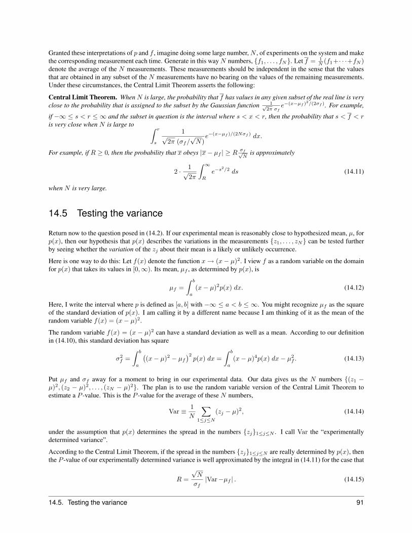
Granted these interpretations of p and f , imagine doing some large number,N , of experiments on the system and makethe corresponding measurement each time. Generate in this wayN numbers, {f1, . . . , fN}. Let f = 1

N (f1+· · ·+fN )denote the average of the N measurements. These measurements should be independent in the sense that the valuesthat are obtained in any subset of the N measurements have no bearing on the values of the remaining measurements.Under these circumstances, the Central Limit Theorem asserts the following:

Central Limit Theorem. WhenN is large, the probability that f has values in any given subset of the real line is veryclose to the probability that is assigned to the subset by the Gaussian function 1√

2π σfe−(x−µf )2/(2σf ). For example,

if −∞ ≤ s < r ≤ ∞ and the subset in question is the interval where s < x < r, then the probability that s < f < ris very close when N is large to ∫ r

s

1√2π (σf/

√N)

e−(x−µf )/(2Nσf ) dx.

For example, if R ≥ 0, then the probability that x obeys |x− µf | ≥ R σf√N

is approximately

2 · 1√2π

∫ ∞R

e−s2/2 ds (14.11)

when N is very large.

14.5 Testing the variance

Return now to the question posed in (14.2). If our experimental mean is reasonably close to hypothesized mean, µ, forp(x), then our hypothesis that p(x) describes the variations in the measurements {z1, . . . , zN} can be tested furtherby seeing whether the variation of the zj about their mean is a likely or unlikely occurrence.

Here is one way to do this: Let f(x) denote the function x→ (x− µ)2. I view f as a random variable on the domainfor p(x) that takes its values in [0,∞). Its mean, µf , as determined by p(x), is

µf =∫ b

a

(x− µ)2p(x) dx. (14.12)

Here, I write the interval where p is defined as [a, b] with −∞ ≤ a < b ≤ ∞. You might recognize µf as the squareof the standard deviation of p(x). I am calling it by a different name because I am thinking of it as the mean of therandom variable f(x) = (x− µ)2.

The random variable f(x) = (x − µ)2 can have a standard deviation as well as a mean. According to our definitionin (14.10), this standard deviation has square

σ2f =

∫ b

a

((x− µ)2 − µf

)2p(x) dx =

∫ b

a

(x− µ)4p(x) dx− µ2f . (14.13)

Put µf and σf away for a moment to bring in our experimental data. Our data gives us the N numbers {(z1 −µ)2, (z2 − µ)2, . . . , (zN − µ)2}. The plan is to use the random variable version of the Central Limit Theorem toestimate a P -value. This is the P -value for the average of these N numbers,

Var ≡ 1N

∑1≤j≤N

(zj − µ)2, (14.14)

under the assumption that p(x) determines the spread in the numbers {zj}1≤j≤N . I call Var the “experimentallydetermined variance”.

According to the Central Limit Theorem, if the spread in the numbers {zj}1≤j≤N are really determined by p(x), thenthe P -value of our experimentally determined variance is well approximated by the integral in (14.11) for the case that

R =√N

σf|Var−µf | . (14.15)

14.5. Testing the variance 91

To summarize: Our hypothetical probability function p(x) gives the expected variance, this the number that we com-pute in (14.12). The Central Limit Theorem then says that our experimentally determined variance, this the numberfrom (14.14), should approach the predicted one in (14.12) asN →∞. Moreover, the Central Limit Theorem gives anapproximate probability, this the expression given using (14.15) in (14.11), for any measured variance to differ fromthe theoretical one by more than the experimentally determined variance. In particular, if the integral in (14.11) is lessthan 1

20 using R from (14.15), then there is a significant chance that our theoretically determined p(x) is not correct.

I am hoping that the example using the values of sin(x) on the integers makes this less abstract. To return to thisexample, recall that the probability function p(x) I use is the uniform probability function on the interval [−1, 1]. Thisversion of p(x) finds µ = 0 and µf = 1

3 for the case f(x) = (x− µ)2 = x2. The relevant version version of (14.13)uses a = −1, b = 1 and p(x) = 1

2 ; and the resulting integral in (14.13) finds σ2f = 4

45 ≈ 0.089. Meanwhile,the N = 100 and xk = sin(k) version of (14.14) finds Var ≈ 0.503. Granted this, then I find the right hand sideof (14.15) equal to 5.69. Since this value for R is larger than

√2, I can use (14.8) as an upper bound for the value of

the integral in (14.11). This upper bound is less than 4.2×10−7! This is an upper bound for the P -value of the numberVar ≈ 0.503 under the hypothesis that the values of {sin(k)}1≤k≤100 are distributed uniformly in the interval [−1, 1].This tiny P -value puts a very dark cloud over my hypothesis that the values of sin(x) for x an integer are uniformlydistributed between −1 and 1.

14.6 Did Gregor Mendel massage his data?

To reach conclusions about inheritance, Gregor Mendel ran a huge number of experiments on pea plants1 In fact,he raised over 20, 000 plants from seed over an 8 year period. From this data, he was able to glean the “simple”inheritance of dominant-recessive genes. In modern language, here is what this means: Some traits are controlled bytwo different versions of a particular gene. The different versions are called “alleles”. One allele gives the “dominant”trait or phenotype, and one gives the “recessive” trait. An individual plant has 2 copies of each gene, and shows therecessive trait only when both the copies are the recessive allele. Each pollen grain receives only one gene, and eachovule receives only one. A seed is formed when a pollen grain merges with an ovule; thus each offspring has againtwo copies of the gene. Granted this fact, if it is assumed that each allele has probability to be passed to any givenpollen grain or ovule, one should expect about a 3:1 ratio of dominant phenotypes to recessive phenotypes.

This explanation for the inheritance of traits from parent plant to seedling predicts also predicts the following: Aindividual plant with the dominant phenotype should have 2 dominant alleles of the time; the other of the time shouldhave one copy of each of the two alleles. A plant with the dominant trait is called a “homozygous” dominant when ithas two dominant alleles, and it is called a “heterozygous” dominant when it has one dominant allele and one recessiveallele. For hundreds of dominant phenotype plants, Mendel was able to classify whether they were homozygous orheterozygous by noting whether the given plant’s clonal offspring (the plant was self-pollinated) showed any recessivetraits. From these experiments, the theory predicts a 2:1 ratio of heterozygous dominant to homozygous dominantplants. Below is a chart of data from Mendel’s work with regards to this homozygous/heterozygous experiment.

Mendel was accused, long after he died, of having massaged his data. One of the complains was that Mendel’s datadoes not have enough spread about the mean. R. A. Fisher2 analyzed this complaint along the following lines: Imagineflipping a coin some number, say N times. Here, the coin is such that the probability of heads is 1

3 . Use the q = 13

binomial probability functions to see that the mean number of heads for N flips is N3 and the standard deviation is

13

√2N . Now, consider Mendel’s data as presented above. There are 8 separate experiments, where the values of N

differ. In particular, the values of the mean and the standard deviation for the 8 different values of N are: Here, I haverounded µ and σ off to the nearest integer. The column that is headed as “h”, is a copy of the column that is headed by“Homozygous Dominant” in the previous table. Thus, this column contains the actual data, the number of homozygousdominant offspring. The far right column takes the number of homozygous dominant offspring, subtracts the mean,divides the result by σ and, after taking absolute values, rounds to the nearest 10th. For example, the number in the farright column for round/wrinkled seeds is 193−188

11 = 511 ≈ 0.5. The number in the far right column for green/yellow

seeds is 173−16610.7 ≈ 0.7. Thus, the far right column gives the distance of the observed value from the expected value

1Mendel, G., 1866 Versuche uber Pflanzen-Hybriden. Verh. Naturforsch. Ver. Brunn 4: 3–47 (first English translation in 1901, J. R. Hortic.Soc. 26: 1–32; reprinted in Experiments in Plant Hybridization, Harvard University Press, Cambridge, MA, 1967).

2Fisher, R. A., 1936, Has Mendel’s work been rediscovered? Ann. Sci. 1: 115–137.


Homozygous HeterozygousDominant Dominant Ratio

round/wrinkled seed 193 372 1.93green/yellow seed 166 353 2.13

colored/white flower 36 64 1.78tall/dwarf plant 28 72 2.57

constricted pod or not 29 71 2.45green/yellow pod #1 40 60 1.50

terminal flower or not 33 67 2.03yellow/green pod #2 35 65 1.86

Total 560 1124 2.01

Table 14.1: Tests of Heterozygosity of Dominant Trait Phenotypes

N µ σ h |h− µ|/σround/wrinkled seed 565 188 11 193 0.5green/yellow seed 519 173 11 166 0.6

colored/white flower 100 33 5 36 0.6tall/dwarf plant 100 33 5 28 1

constricted pod or not 100 33 5 29 0.8green/yellow pod #1 100 33 5 40 1.4

terminal flower or not 100 33 5 33 0yellow/green pod #2 100 33 5 35 0.4

as measured in units where 1 means 1 standard deviation.

Those who complained about the spread of Mendel’s data presumably made a table just like the one just given, andthen noticed the following interesting fact: In 7 of the 8 cases, the observed value for h has distance less than or equalto 1 standard deviation from the mean. They must have thought that this clustering around the mean was not likely toarise by chance.

What follows describes a method to estimate a P -value for having 7 of 8 measurements land within one standarddeviation of the mean. To do this invoke the Central Limit theorem in each of the eight cases to say that the probabilitythat h has a given value, say x, should be determined to great accuracy by the Gaussian probability function:

p(x) =1√

2π σe−(x−µ)2/(2σ2). (14.16)

Granted that the Central Limit theorem is applicable, then the probability of h having value within 1 standard deviationfrom the mean is

q =∫ µ+σ

µ−σ

1√2π σ

e−(x−µ)2/(2σ2) dx ≈ 0.68. (14.17)

This has the following consequence: The probability of getting n ∈ {0, 1, . . . , 8} out of 8 measurements to liewithin 1 standard deviation is given by the N = 8 binomial probability function using q = 0.68. This is p(n) =

8!n! (8−n)! (0.68)n(0.32)8−n. Note that the mean this binomial function is 8(0.68) = 5.44. Thus, the P -value forgetting 7 of 8 measurements within 1 standard deviation of the mean is

p(0) + p(1) + p(2) + p(3) + p(7) + p(8).

As it turns out this ≈ 0.58, thus greater than 0.05.

Looking back on this discussion, note that I invoked binomial probability functions in two different places. The firstwas to derive the right most column in the table. This used a q = 1

3 binomial with values of N given by the left-mostcolumn of numbers in the table. The value of came from the hypothesis about the manner in which genes are passedfrom parent plant to seedling. The second application of the binomial probability function used the q = 0.68 versionwithN = 8. I used this version to compute a P -value for having 7 of 8 measurements land within 1 standard deviationof the mean. The value 0.68 for q was justified by an appeal to the Central Limit theorem.

14.6. Did Gregor Mendel massage his data? 93

14.7 Boston weather 2008

This last part of the chapter briefly discusses a case where hypothesis testing might say something interesting. Thefollowing chart from the Sunday, January 4 New York Times gives the daily temperature extremes in Boston for theyear 2008: The chart claims that the average temperature for the year was 0.5 degrees above normal. The grayish

Figure 14.1: Temperature Extremes in Boston (NY Times, Sunday, January 4, 2009)

swath in the background is meant to indicate the “normal range”. (Nothing is said about what this means.)

We hear all the time about “global warming”. Does this chart give evidence for warming in Boston during the year2008? What follows describe what may be an overly simplistic way to tease some answer to this question from thechart. Let us assume that the center of the grey swath on each day represents the mean temperature on the givenday as computed by averaging over some large number of years. This gives us an ordered set of 366 numbers,{T1, . . . , T366}. Meanwhile, the chart gives us, for each day in 2008, the actual mean temperature on that day, thishalf of the sum of the indicated high and low temperature on that day. This supplies us with a second sequence of 366numbers, {t1, . . . , t366}. Subtracting the first sequence from the second gives us numbers (x1 = t1 − T1, . . . , x366 =t366 − T366). Take this set of 366 numbers to be the experimentally measured data.

The chart tells us that the average, µreal = 1366 (x1 + · · · + x366), of the experimental data is equal to 0.5. We can

then ask if this average is consistent with the hypothesis that the sequence (x1, . . . , x366) is distributed according to aGaussian distribution with mean zero and some as yet unknown standard deviation. Unfortunately, the chart doesn’tsay anything about the standard deviation. This understood, let us proceed with the assumption that the standarddeviation is half the vertical height of the grey swath, which is to say roughly 6◦ degrees Fahrenheit. If we make thisassumption, then we are comparing the number 0.5 with what would be expected using the Central Limit theorem withinput a Gaussian with mean zero and standard deviation 6◦. The Central Limit theorem asserts that the P -value of themeasured mean 0.5 as computed using N = 366 and this hypothetical Gaussian is ≈ 0.14, which is not significant.

We can also ask whether the variance of the data set (x1, . . . , x366) is consistent with the assumption that thesenumbers are distributed according a Gaussian with mean µ = 0 and standard deviation σ = 6◦. This is to say that weare comparing the experimentally variance σ2

real = 1366 (x2

1 + · · · + x2366) with the average of 366 distances from the

mean as computed using the Central Limit theorem for the Gaussian with mean µ = 0 and σ = 6◦.


Of course, we can go further. For example, when I look at the graph, I sense that there are more peaks that are verymuch above the grey swath than there are peaks that are very much below the grey swath. I can test whether this isconsistent with the Gaussian assumption by using the central limit theorem for the average of N = 366 measurementsof the random variable f(x) = 1

2 (x+ |x|). (Note that f(x) = 0 when x ≤ 0 and f(x) = x when x > 0.)

14.8 Exercises:

1. Suppose that we expect that the x-coordinate of bacteria in our rectangular petri dish should be any valuebetween −1 and 1 with equal probability in spite of our having coated the x = 1 wall of the dish with a specificchemical. We observe the positions of 900 bacteria in our dish and so obtain 900 values, {z1, . . . , z900}, for thex-coordinates.

(a) Suppose the average, z = 1900

∑1≤k≤900 zk, is 0.1. Use the Central Limit Theorem to obtain a theoretical

upper bound based on our model of a uniform probability function for the probability that an average of900 x-coordinates differs from 0 by more than 0.1.

(b) Suppose that the average of the squares, Var =∑

1≤k≤900 z2k, equals 0.36. Use the Central Limit Theorem

and (13.21) to obtain a theoretical upper bound based on our model of a uniform probability function forthe probability that an average of the squares of 900 x-coordinates is greater than or equal to 0.36. (Notethat I am not asking that it differ by a certain amount from the square of the standard deviation for theuniform probability function. If you compute the latter, you will be wrong by a factor of 2.)

2. Use Stirling’s formula in Equation (11.14) to give approximate formulae for both (2k)!k!2k

and 12k

((2k)!k! −

(k!k2 !

)2)

when k is large.

3. R. A. Fisher (see also reference2 above) discussed a second criticism of Mendel’s experimental data. Thisinvolved the manner in which a given dominant phenotype plant was classified as being “homozygous dominant”or “heterozygous dominant”. According to Fisher, Mendel used the following method on any given plant: Hegerminated 10 seeds from the plant via self-pollination, and if all 10 of the resulting seedlings had the dominantphenotype, he then labeled the plant as “homozygous dominant”. If one or more of the 10 seedlings had therecessive phenotype, he labeled the plant as “heterozygous dominant”. Fisher pointed out that if Mendel reallydid the classification in this manner, then he should have mislabeled some heterozygous dominant plants ashomozygous dominant. The following questions walk you through some of Fisher’s arguments.

(a) What is the probability for a heterozygous dominant plant to produce a seedling with the dominant pheno-type?

(b) What binomial probability function should you use to compute the probability that a heterozygous plantproduces 10 consecutive dominant seedlings.

(c) Use the binomial probability function for (b) to compute the probability of any given heterozygous domi-nant plant to produce 10 consecutive dominant seedlings.

(d) If any given plant has probability to be homozygous dominant and thus to be heterozygous dominant, whatis the probability that Mendel would label any given plant as “homozygous dominant”? (To answer this,you can use conditional probabilities. To this end, suppose that you have a sample space of N plants.Use A to denote the subset of plants that are homozygous dominant, B to denote the subset that areheterozygous dominant, and C to denote the subset that Mendel designates are homozygous dominant.)

(e) Redo the second table in this chapter based on your answer to (c) of this chapter.

4. The 2006 election for the United States Senator in Virginia had the following outcome (according to cnn.com):

Webb: 1, 172, 671 votesAllen: 1, 165, 440 votes

14.8. Exercises 95

cnn.com

The total votes cast for the two candidates was 2, 238, 111, and the difference in the vote totals was 7, 231. Thiswas considered by the press to be an extremely tight election. Was it unreasonably close? Suppose that anelection to choose one of two candidates is held with 2, 238, 111 voters. Suppose, in addition, that each votercasts his or her vote at random. If you answer correctly the questions (b) and (c) below, you will obtain anestimate for the probability as determined by this “vote at random” model that the difference between the twocandidates is less than or equal to 7, 231.

(a) Set N = 2, 238, 111. Let S denote the sample space whose elements are sequences of the form{z1, . . . , zN} where each zk is either 1 or −1. Use f to denote the random variable on S that is givenby the formula f(z1, . . . , zN ) = z1 + z2 + · · ·+ zN . What is the mean and what is the standard deviationof f?

(b) Use the Central Limit Theorem to find a Gaussian probability function that can be used to estimate theprobability that 1

N f has value in any given interval on the real line.

(c) Use the Gaussian probability from (b) to compute the probability that | 1N f | ≤

7,231N . Note that this is

the probability (as computed by this Gaussian) for |f | to be less than or equal to 7, 231. (You can use acalculator if you like to compute the relevant integral.)


CHAPTER

FIFTEEN

Determinants

This chapter is meant to provide some cultural background to the story told in the linear algebra text book aboutdeterminants. As the text explains, the determinant of a square matrix is non-zero if and only if the matrix is invertible.The fact that the determinant signals invertibility is one of its principle uses. The other is the geometric fact observedby the text that the absolute value of the determinant of the matrix is the factor by which the linear transformationexpands or contracts n-dimensional volumes. This chapter considers an invertibility question of a biological sort, anapplication to a protein folding problem.

Recall that a protein molecule is a long chain of smaller molecules that are tied end to end. Each of these smallermolecules can be any of twenty so called amino acids. This long chain appears in a cell folded up on itself in acomplicated fashion. In particular, its interactions with the other molecules in the cell are determined very much bythe particular pattern of folding because any given fold will hide some amino acids on its inside while exhibiting otherson the outside. This said, one would like to be able to predict the fold pattern from knowledge of the amino acid thatoccupies each site along the chain.

In all of this, keep in mind that the protein is constructed in the cell by a component known as a “ribosome”, andthis construction puts the chain together starting from one end by sequentially adding amino acids. As the chain isconstructed, most of the growing chain sticks out of the ribosome. If not stabilized by interactions with surroundingmolecules in the cell, a given link in the chain will bend this way or that as soon as it exits the ribosome, and so theprotein would curl and fold even as it is constructed.

To get some feeling for what is involved in predicting the behavior here, make the grossly simplifying assumptionthat each of the amino acids in a protein molecule of length N can bend in one of 2 ways, but that the probability ofbending, say in the + direction for the nth amino acid is influenced by the direction of bend of its nearest neighbors,the amino acids in sites n− 1 and n+ 1. One might expect something like this for short protein molecules in as muchas the amino acids have electrical charges on them and so feel an electric force from their neighbors. As this force isgrows weaker with distance, their nearest neighbors will affect them the most. Of course, once the chain folds backon itself, a given amino acid might find itself very close to another that is actually some distance away as measured bywalking along the chain.

In any event, let us keep things very simple and suppose that the probability, pn(t), at time t of the nth amino acidbeing in the + fold position evolves as

pn(t+ 1) = an +An,npn(t) +An,n−1pn−1(t) +An,n+1pn+1(t). (15.1)

Here, an is some fixed number between 0 and 1, and the numbers {an, An,n, An,n±1} are constrained so that

0 ≤ an +An,nx+An,n−1 x− +An,n+1x+ ≤ 1 (15.2)

for any choice between 0 and 1 of values for x, x− and x+ with x + x− + x+ ≤ 1. This constraint is necessary toguarantee that pn(t + 1) is between 0 and 1 if each of pn(t), pn+1(t) and pn−1(t) is between 0 and 1. In this regard,let me remind you that pn(t + 1) must be between 0 and 1 if it is the probability of something. My convention heretakes both A1,0 and AN,N+1 to be zero.

As for the values of the other coefficients, I will suppose that knowledge of the amino acid type that occupies site n

97

is enough to determine an and Ann, and that knowledge of the respective types that occupy sites n − 1 and n + 1 isenough to determine An,n−1 and An,n+1. In this regard, I assume access to a talented biochemist.

Granted these formulæ, the N -component vector ~p(t) whose nth component is pn(t) evolves according to the rule:

~p(t+ 1) = ~a+A~p(t) (15.3)

where ~a is that N -component vector whose nth entry is an, and where A is that N ×N matrix whose only non-zeroentries are {An,n, An,n±1}1≤n≤N .

We might now ask if there exists an equilibrium probability distribution, anN -component vector, ~p, with non-negativeentries that obeys

~p = ~a+A~p (15.4)

If there is such a vector, then we might expect its entries to give us the probabilities for the bending directions of thevarious links in the chain for the protein. From this, one might hope to compute the most likely fold pattern for theprotein.

To analyze (15.4), let us rewrite it as the equation

(I −A)~p = ~a, (15.5)

where I here denotes the identity matrix; this the matrix with its only entries on the diagonal and with all of the latterequal to 1. We know now that there is some solution, ~p, when det(I − A) 6= 0. It is also unique in this case. Indeed,were there two solutions, ~p and ~p′, then

(I −A)(~p− ~p′) = 0. (15.6)

This implies (I −A) has a kernel, which is forbidden when I −A is invertible. Thus, to understand this version of theprotein folding problem, we need to consider whether the matrix I −A is invertible. As remarked at the outset, this isthe case if and only if it has non-zero determinant.

By the way, we must also confirm that the solution, ~p, to (15.5) has its entries between 0 and 1 so as to use the entriesas probabilities.

In any event, to give an explicit example, consider the 3× 3 case. In this case, the matrix I −A is1−A11 −A12 0−A21 1−A12 −A23

−A31 −A32 1−A12

. (15.7)

Using the formulae from Chapter 6 of the linear algebra text book, its determinant is found to be

det(I −A) = (1−A11)(1−A22)(1−A33)− (1−A11)A23A32 − (1−A33)A12A21. (15.8)

98 Chapter 15. Determinants

CHAPTER

SIXTEEN

Eigenvalues in biology

My goal in this chapter is to illustrate how eigenvalues can appear in problems from biology.

16.1 An example from genetics

Suppose we have a fixed size N population of cells that reproduce by fission. The model here is that there are N cellsthat divide at the start, thus producing 2N cells. After one unit of time, half of these die and half survive, so there areN cells to fission at the end of 1 unit of time. These N survivors divide to produce 2N cells and so start the next runof the cycle. In particular, there are always N surviving cells at the end of one unit of time and then 2N just at thestart of the next as each of these N cells splits in half.

Now, suppose that at the beginning, t = 0, there is, for each n ∈ {0, 1, . . . , N}, a given probability which I’ll callpn(0) for n of the N initial cells to carry a certain trait. Suppose that this trait (red color as opposed to blue) is neutralwith respect to the cell’s survival. In other words, the probability is for any given red cell to survive to reproduce, andthe probability is for any given blue cell to survive to reproduce.

Here is the key question: Given the initial probabilities, {p0(0), p1(0), . . . , pN (0)}, what are the corresponding prob-abilities after some t generations? Thus, what are the values of {p0(t), p1(t), . . . , pN (t)} where now pn(t) denotesthe probability that n cells of generation t carry the red color?

To solve this, we can use our tried and true recourse to conditional probabilities by noting that

pn(t) = P (n red survivors | 0 red parents) · p0(t− 1)+ P (n red survivors | 1 red parent) · p1(t− 1) (16.1)+ P (n red survivors | 2 red parents) · p2(t− 1) + · · ·

where P (n red survivors |m red parents) is the conditional probability that there are n red cells at the end of a cyclegiven that there werem such cells the end of the previous cycle. If the ambient environmental conditions don’t change,one would expect that these conditional probabilities are independent of time. As I explain below, they are, in fact,computable from what we are given about this problem. In any event, let me use the shorthand A to denote the squarematrix of size N + 1 whose entry in row n and column m is P (n red survivors |m red parents). In this regard, notethat n and m run from 0 to N , not the from 1 to N + 1. Let ~p(t) denote the vector in RN+1 whose nth entry is pn(t).Then (16.1) reads

~p(t) = A~p(t− 1). (16.2)

This last equation would be easy to solve if we knew that ~p(0) was an eigenvector of the matrix A. That is, if it werethe case that

A~p(0) = λ~p(0) with λ some real number. (16.3)

Indeed, were this the case, then the t = 1 version of (16.2) would read ~p(1) = λ~p(0). We could then use the t = 2version of (16.2) to compute ~p(2) and we would find that ~p(2) = λA~p(0) = λ2~p(0). Continuing in the vein, we wouldfind that ~p(t) = λt~p(0) and our problem would be solved.

99

Now, it is unlikely that ~p(0) is going to be an eigenvector. However, even if ~p(0) is a linear combination of eigenvectors,

~p(0) = c1~e1 + c2~e2 + · · · , (16.4)

we could still solve for ~p(t). Indeed, let λk denote the eigenvalue for any given ~ek. Thus, A~ek = λk~ek. Granted weknow these eigenvalues and eigenvectors, then we can plug (16.4) into the t = 1 version of (16.2) to find

~p(1) = c1λ1~e1 + c2λ2~e2 + · · · . (16.5)

We could then plug this into the t = 2 version of (16.2) to find that

~p(2) = c1λ21~e1 + c2λ

22~e2 + · · · , (16.6)

and so on. In general, this then gives~p(t) = c1λ

t1~e1 + c2λ

t2~e2 + · · · . (16.7)

16.2 Transition/Markov matrices

The matrix A that appears in (16.2) has entries that are conditional probabilities, and this has the following implica-tions:

• All entries are non-negative.

• A0,m +A1,m + · · ·+AN,m = 1 for all m ∈ {0, 1, . . . , N}.(16.8)

The last line above asserts that the probability is 1 of there being some number, either 0 or 1 or 2 or . . . or N of redcells in the subsequent generation given m red cells in the initial generation.

A square matrix with this property is called a transition matrix, or sometimes a Markov matrix. When A is such amatrix, the equation in (16.2) is called a Markov process.

Although we are interested in the eigenvalues of A, it is amusing to note that the transpose matrix, AT , has aneigenvalue equal to 1 with the corresponding eigenvector being proportional to the vector, ~a, with each entry equal to1. Indeed, the entry in the mth row and nth column of AT is Anm, this the entry of A in the nth row and mth column.Thus, the mth entry of AT~a is

(AT~a)m = A0,ma0 +A1,ma1 + · · ·+AN,maN . (16.9)

If the lower line in (16.10) is used and if each ak is 1, then each entry of AT~a is also 1. Thus, AT~a = ~a.

As a “cultural” aside, what follows is the story on Anm in the example from Section 16.1. First, Anm = 0 if n islarger than 2m since m parent cells can spawn at most 2m survivors. For n ≤ m, consider that you have 2N cells ofwhich 2m are red and you ask for the probability that a choice of N from the 2N cells results in n red ones. This is acounting problem that is much like those discussed in Section 11.3 although more complicated. The answer here is:

Anm =(N !)2

(2N)!(2m)!

n! (2m− n)!(2N − 2m)!

(N −m)! (N + n− 2m)!when 0 ≤ n ≤ 2m. (16.10)

16.3 Another protein folding example

Here is another model for protein folding. As you may recall from previous chapters, a protein is made of segmentstied end to end as a chain. Each segment is one of 20 amino acids. The protein is made by the cell in a large andcomplex molecule called a ribosome. The segments are attached one after the other in the ribosome and so the chaingrows, link by link. Only a few segments are in the ribosome, and the rest stick out as the protein grows. As soonas a joint between two segments is free of the ribosome, it can bend if it is not somehow stabilized by surrounding

100 Chapter 16. Eigenvalues in biology

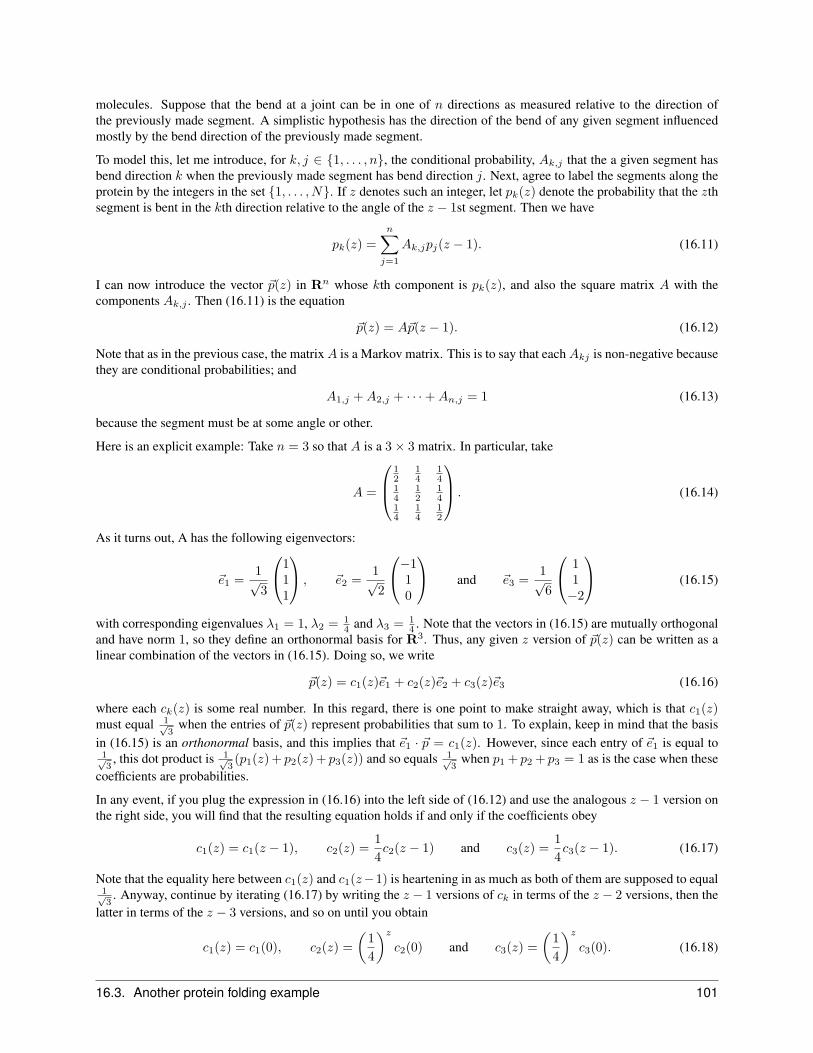
molecules. Suppose that the bend at a joint can be in one of n directions as measured relative to the direction ofthe previously made segment. A simplistic hypothesis has the direction of the bend of any given segment influencedmostly by the bend direction of the previously made segment.

To model this, let me introduce, for k, j ∈ {1, . . . , n}, the conditional probability, Ak,j that the a given segment hasbend direction k when the previously made segment has bend direction j. Next, agree to label the segments along theprotein by the integers in the set {1, . . . , N}. If z denotes such an integer, let pk(z) denote the probability that the zthsegment is bent in the kth direction relative to the angle of the z − 1st segment. Then we have

pk(z) =n∑j=1

Ak,jpj(z − 1). (16.11)

I can now introduce the vector ~p(z) in Rn whose kth component is pk(z), and also the square matrix A with thecomponents Ak,j . Then (16.11) is the equation

~p(z) = A~p(z − 1). (16.12)

Note that as in the previous case, the matrixA is a Markov matrix. This is to say that eachAkj is non-negative becausethey are conditional probabilities; and

A1,j +A2,j + · · ·+An,j = 1 (16.13)

because the segment must be at some angle or other.

Here is an explicit example: Take n = 3 so that A is a 3× 3 matrix. In particular, take

A =

12

14

14

14

12

14

14

14

12

. (16.14)

As it turns out, A has the following eigenvectors:

~e1 =1√3

111

, ~e2 =1√2

−110

and ~e3 =1√6

11−2

(16.15)

with corresponding eigenvalues λ1 = 1, λ2 = 14 and λ3 = 1

4 . Note that the vectors in (16.15) are mutually orthogonaland have norm 1, so they define an orthonormal basis for R3. Thus, any given z version of ~p(z) can be written as alinear combination of the vectors in (16.15). Doing so, we write

~p(z) = c1(z)~e1 + c2(z)~e2 + c3(z)~e3 (16.16)

where each ck(z) is some real number. In this regard, there is one point to make straight away, which is that c1(z)must equal 1√

3when the entries of ~p(z) represent probabilities that sum to 1. To explain, keep in mind that the basis

in (16.15) is an orthonormal basis, and this implies that ~e1 · ~p = c1(z). However, since each entry of ~e1 is equal to1√3

, this dot product is 1√3(p1(z) + p2(z) + p3(z)) and so equals 1√

3when p1 + p2 + p3 = 1 as is the case when these

coefficients are probabilities.

In any event, if you plug the expression in (16.16) into the left side of (16.12) and use the analogous z − 1 version onthe right side, you will find that the resulting equation holds if and only if the coefficients obey

c1(z) = c1(z − 1), c2(z) =14c2(z − 1) and c3(z) =

14c3(z − 1). (16.17)

Note that the equality here between c1(z) and c1(z−1) is heartening in as much as both of them are supposed to equal1√3

. Anyway, continue by iterating (16.17) by writing the z − 1 versions of ck in terms of the z − 2 versions, then thelatter in terms of the z − 3 versions, and so on until you obtain

c1(z) = c1(0), c2(z) =(

14

)zc2(0) and c3(z) =

(14

)zc3(0). (16.18)

16.3. Another protein folding example 101

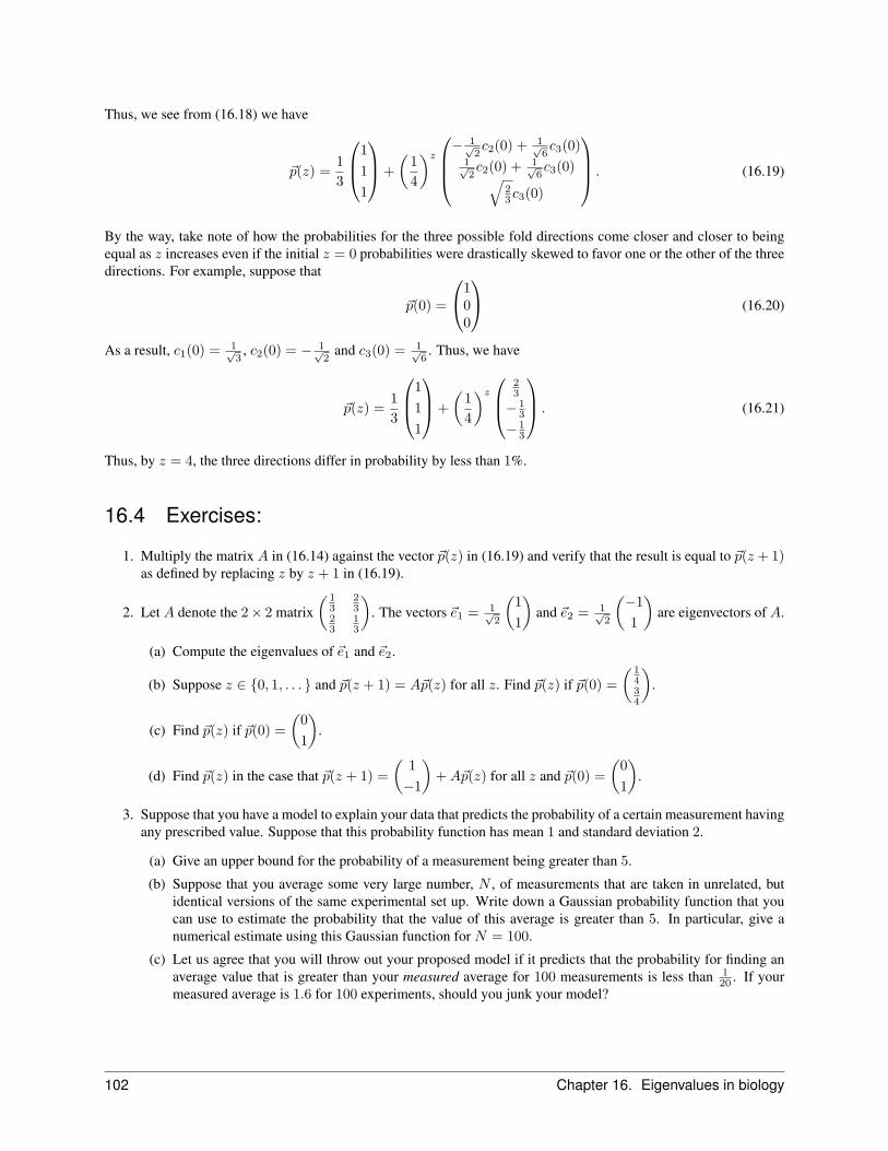
Thus, we see from (16.18) we have

~p(z) =13

111

+(

14

)z− 1√

2c2(0) + 1√

6c3(0)

1√2c2(0) + 1√

6c3(0)√

23c3(0)

. (16.19)

By the way, take note of how the probabilities for the three possible fold directions come closer and closer to beingequal as z increases even if the initial z = 0 probabilities were drastically skewed to favor one or the other of the threedirections. For example, suppose that

~p(0) =

100

(16.20)

As a result, c1(0) = 1√3

, c2(0) = − 1√2

and c3(0) = 1√6

. Thus, we have

~p(z) =13

111

+(

14

)z23

− 13

− 13

. (16.21)

Thus, by z = 4, the three directions differ in probability by less than 1%.

16.4 Exercises:

1. Multiply the matrix A in (16.14) against the vector ~p(z) in (16.19) and verify that the result is equal to ~p(z + 1)as defined by replacing z by z + 1 in (16.19).

2. Let A denote the 2× 2 matrix( 1

323

23

13

). The vectors ~e1 = 1√

2

(11

)and ~e2 = 1√

2

(−11

)are eigenvectors of A.

(a) Compute the eigenvalues of ~e1 and ~e2.

(b) Suppose z ∈ {0, 1, . . . } and ~p(z + 1) = A~p(z) for all z. Find ~p(z) if ~p(0) =( 1

434

).

(c) Find ~p(z) if ~p(0) =(

01

).

(d) Find ~p(z) in the case that ~p(z + 1) =(

1−1

)+A~p(z) for all z and ~p(0) =

(01

).

3. Suppose that you have a model to explain your data that predicts the probability of a certain measurement havingany prescribed value. Suppose that this probability function has mean 1 and standard deviation 2.

(a) Give an upper bound for the probability of a measurement being greater than 5.

(b) Suppose that you average some very large number, N , of measurements that are taken in unrelated, butidentical versions of the same experimental set up. Write down a Gaussian probability function that youcan use to estimate the probability that the value of this average is greater than 5. In particular, give anumerical estimate using this Gaussian function for N = 100.

(c) Let us agree that you will throw out your proposed model if it predicts that the probability for finding anaverage value that is greater than your measured average for 100 measurements is less than 1

20 . If yourmeasured average is 1.6 for 100 experiments, should you junk your model?

102 Chapter 16. Eigenvalues in biology

4. Suppose that you repeat the same experiment 100 times and each time record the value of a certain key measure-

ment. Let {x1, . . . , x100} denote the values of the measurement in N experiments. Suppose that100∑k=1

xk = 0

and 199

100∑k=1

x2k = 1. Suppose, in addition, that five of the xk obey xk > 3. The purpose of this problem is to

walk you through a method for obtaining an upper bound for the likelihood of having five measurements that farfrom the mean. In this regard, suppose that you make the hypothesis that the spread of the measured numbers{xk}1≤k≤100 is determined by the Gaussian probability function with mean 0 and standard deviation equal to1.

(a) Let p denote the probability using this Gaussian probability function for a measurement x with x ≥ 3.Explain why p ≤ e−9/2 ≤ 0.0015.

(b) Use the binomial probability function to explain why the probability of finding five or more values for kout of 100 that have xk > 3 is equal to

100∑k=5

100!k! (100− k)!

pk(1− p)100−k.

(c) Let k ≥ 5 and let z → fk(z) = zk(1− z)100−k. Show that f is an increasing function of z when z < 120 .

(Hint: Take its derivative with respect to z.)

(d) Since p ≤ 0.0015 ≤ 0.05 = 120 , use the result from part (c) to conclude that the probability of finding 5 or

more of the xk’s out of 100 with xk > 3 has probability less than

100∑k=5

(0.0015)k(0.9985)100−k.

(e) We saw in Equation (11.19) of Chapter 11 that the terms in the preceding sum get ever smaller as kincreases. Use a calculator to show that the k = 5 term and thus all higher k terms are smaller than5× 10−7. Since there are less than 95 ≤ 100 of these terms prove that the sum of these terms is no greaterthan 0.00005.

16.4. Exercises 103

CHAPTER

SEVENTEEN

More about Markov matrices

The notion of a Markov matrix was introduced in Chapter 15. By way of a reminder, this is an N ×N matrix A thatobeys the following conditions:

• Ajk ≥ 0 for all j and k.

• A1k +A2k + · · ·+ANk = 1 for all k.(17.1)

These two conditions are sufficient (and also necessary) for the interpretation of the components of A as conditionalprobabilities. To this end, imagine a system with N possible states, labeled by the integers starting at 1. Then Ajk canrepresent the conditional probability that the system is in state j at time t if it is in state k at time t− 1. In particular,one sees Markov matrices arising in a dynamical system where the probabilities for the various states of the system atany given time are represented by an N -component vector, ~p(t), that evolves in time according to the formula

~p(t) = A~p(t− 1). (17.2)

Here is a 3× 3 Markov matrix 14

13

16

12

13

23

14

13

16

. (17.3)

All entries are non-negative, and the entries in each column sum to 1. Note that there is no constraint for the sum ofthe entries in any given row.

A question that is often raised in the general context of (17.1) and (17.2) is whether the system has an equilibriumprobability function, thus some non-zero vector ~p∗, with non-negative entries that sum to 1, and that obeys A~p∗ = ~p∗.If so, there is the associated question of whether the t→∞ limit of ~p(t) must necessarily converge to the equilibrium~p∗.

104

Here are some facts that allow us to answer these questions.

• Any Markov matrix always has an eigenvector with eigenvalue 1.

• If each entry of a Markov matrix A is strictly positive, then every non-zero vectorin the kernel of A − I has either all positive entries or all negative entries. Here, Idenotes the identity matrix.

• If each entry of a Markov matrix A is strictly positive, there is a vector in the kernelof the matrix A− I whose entries are positive and sum to 1.

• If each entry of a Markov matrix A is strictly positive, then the kernel of A − I isone dimensional. Furthermore, there is unique vector in the kernel of A − I whoseentries are positive and sum to 1.

• If each entry ofA is strictly positive, all other eigenvalues have absolute value strictlyless than 1. Moreover, the entries of any eigenvector for an eigenvalue that is lessthan 1 must sum to zero.

(17.4)

I elaborate on these points in Section 17.2, below. Accept them for the time being.

17.1 Solving the equation

Let me suppose that A is a Markov matrix and that none of its entries are zero. This allows me to use all of the factsthat are stated in (17.4). Let me also suppose that A has a basis of eigenvectors. In this case, (17.2) can be solvedusing the basis of eigenvectors. To make this explicit, I denote this basis of eigenvectors as {~e1, . . . , ~en} and I use λkto denote the eigenvector of ~ek. Here, my convention has λ1 = 1 and I take ~e1 to be the eigenvector with eigenvalue1 whose entries sum to 1. Note that I am using the first four facts in (17.4) to conclude that A must have a uniqueeigenvector with eigenvalue 1 and positive entries that sum to 1.

Now, the solution to (17.2) depends on the starting vector, ~p(0). In the context where this is a vector of probabilities,it can not have a negative entry. Moreover, its entries must sum to 1. As explained below, this requires that

~p(0) = ~e1 +n∑k=2

ck~ek. (17.5)

The point is that the coefficient in front of ~e1 is necessarily equal to 1. The coefficient, ck, in front of any k ≥ 2version of ~ek is not so constrained.

Here is why (17.5) must hold: In general, I can write ~p(0) = c1~e1 +∑nk=2 ck~ek where c1, c2, . . . , cn are real numbers

because I am assuming that A is diagonalizable, and the eigenvectors of any diagonalizable matrix comprise a basis. Itfollows from this representation of ~p(0) that the sum of its entries is obtained by adding the following numbers: First,c1 times the sum of the entries of ~e1, then c2 times the sum of the entries ~e2, then c3 times the sum of the entries of~e3, and so on. However, the last point of (17.4) asserts that the sum of the entries of each k ≥ 2 version of ~ek is zero.This means that the sum of the entries of ~p(0) is c1 times the sum of the entries of ~e1. Since the sum of the entries of~e1 is 1 and since this is also the sum of the entries of ~p(0), so c1 must equal 1. This is what is asserted by (17.5).

By way of an example, consider the 2× 2 case where

A =[ 1

412

34

12

]. (17.6)

The eigenvalues in this case are 1 and − 14 and the associated eigenvectors ~e1 and ~e2 in this case can be taken to be

~e1 =[ 2

535

]and ~e2 =

[1−1

]. (17.7)

17.1. Solving the equation 105

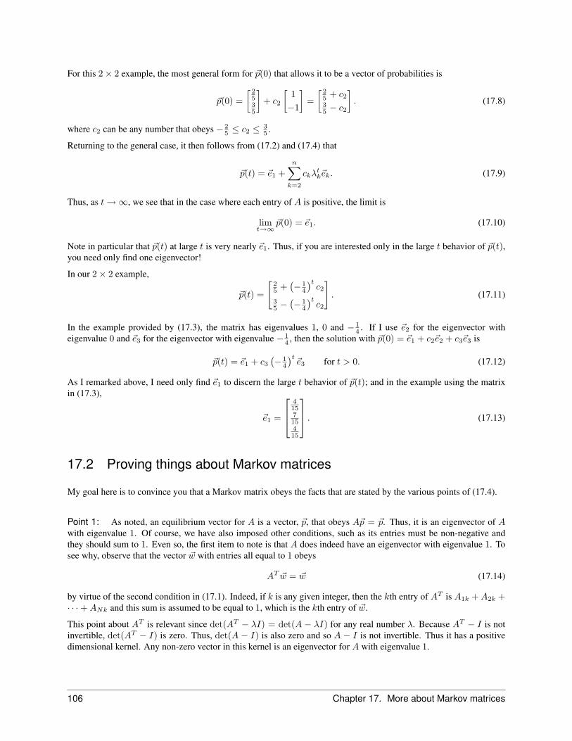
For this 2× 2 example, the most general form for ~p(0) that allows it to be a vector of probabilities is

~p(0) =[ 2

535

]+ c2

[1−1

]=[ 2

5 + c235 − c2

]. (17.8)

where c2 can be any number that obeys − 25 ≤ c2 ≤

35 .

Returning to the general case, it then follows from (17.2) and (17.4) that

~p(t) = ~e1 +n∑k=2

ckλtk~ek. (17.9)

Thus, as t→∞, we see that in the case where each entry of A is positive, the limit is

limt→∞

~p(0) = ~e1. (17.10)

Note in particular that ~p(t) at large t is very nearly ~e1. Thus, if you are interested only in the large t behavior of ~p(t),you need only find one eigenvector!

In our 2× 2 example,

~p(t) =

[25 +

(− 1

4

)tc2

35 −

(− 1

4

)tc2

]. (17.11)

In the example provided by (17.3), the matrix has eigenvalues 1, 0 and − 14 . If I use ~e2 for the eigenvector with

eigenvalue 0 and ~e3 for the eigenvector with eigenvalue − 14 , then the solution with ~p(0) = ~e1 + c2~e2 + c3~e3 is

~p(t) = ~e1 + c3(− 1

4

)t~e3 for t > 0. (17.12)

As I remarked above, I need only find ~e1 to discern the large t behavior of ~p(t); and in the example using the matrixin (17.3),

~e1 =

415715415

. (17.13)

17.2 Proving things about Markov matrices

My goal here is to convince you that a Markov matrix obeys the facts that are stated by the various points of (17.4).

Point 1: As noted, an equilibrium vector for A is a vector, ~p, that obeys A~p = ~p. Thus, it is an eigenvector of Awith eigenvalue 1. Of course, we have also imposed other conditions, such as its entries must be non-negative andthey should sum to 1. Even so, the first item to note is that A does indeed have an eigenvector with eigenvalue 1. Tosee why, observe that the vector ~w with entries all equal to 1 obeys

AT ~w = ~w (17.14)

by virtue of the second condition in (17.1). Indeed, if k is any given integer, then the kth entry of AT is A1k +A2k +· · ·+ANk and this sum is assumed to be equal to 1, which is the kth entry of ~w.

This point about AT is relevant since det(AT − λI) = det(A − λI) for any real number λ. Because AT − I is notinvertible, det(AT − I) is zero. Thus, det(A − I) is also zero and so A − I is not invertible. Thus it has a positivedimensional kernel. Any non-zero vector in this kernel is an eigenvector for A with eigenvalue 1.

106 Chapter 17. More about Markov matrices

Point 2: I assume for this point that all of A’s entries are positive. Thus, all Ajk obey the condition Ajk > 0. Ihave to demonstrate to you that there is no vector in the kernel of A − I with whose entries are not all positive or allnegative. To do this, I will assume that I have a vector ~v that violates this conclusion and demonstrate why this lastassumption is untenable. To see how this is going to work, suppose first that only the first entry of ~v is zero or negativeand the rest are non-negative with at least one positive. Since ~v is an eigenvector of A with eigenvalue 1,

v1 = A11v1 +A12v2 + · · ·+A1nvn. (17.15)

As a consequence, (17.15) implies that

(1−A11)v1 = A12v2 + · · ·+A1nvn (17.16)

Now, A11 is positive, but it is less than 1 since it plus A21 + A31 + · · · + An1 give 1 and each of A21, . . . , An1 ispositive. This implies that the left-hand side of (17.16) is negative if it were the case that v1 < 0, and it is zero if v1

were equal to zero. Meanwhile, the right-hand side to (17.16) is strictly positive. Indeed, at least one k > 1 versionof vk is positive and its attending A1k is positive, while no k > 1 versions of vk are negative nor are any Ajk. Thus,were it the case that v1 is not strictly positive, then (17.16) equates a negative or zero left-hand side with a positiveright-hand side. Since this is nonsense, I see that I could never have an eigenvector of A with eigenvalue 1 that hadone negative or zero entry with the rest non-negative with one or more positive.

Here is the argument when two or more of the vks are negative or zero and the rest are greater than or equal to zero withat least one positive: Let’s suppose for simplicity of notation that v1 and v2 are either zero or negative, and that rest ofthe vks are either zero or positive. Suppose also that at least one k ≥ 3 version of vk is positive. Along with (17.15),we have

v2 = A21v1 +A22v2 +A23v3 + · · ·+A2nvn. (17.17)

Now add this equation to (17.15) to obtain

v1 + v2 = (A11 +A21)v1 + (A12 +A22)v2 + (A13 +A23)v3 + · · ·+ (A1n +A2n)vn. (17.18)

According to (17.1), the sum A11 +A21 is positive and strictly less than 1 since it plus the strictly positive A31 + · · ·+An1 is equal to 1. Likewise, A21 +A22 is strictly less than 1. Thus, when I rearrange (17.18) as

(1−A11 −A21)v1 + (1−A21 −A22)v2 = (A13 +A23)v3 + · · ·+ (A1n +A2n)vn, (17.19)

I again have an expression where the left-hand side is negative or zero and where the right hand side is greater thanzero. Of course, such a thing can’t arise, so I can conclude that the case with two negative versions of vk and one ormore positive versions can not arise.

The argument for the general case is very much like this last argument so I walk you through it in one of the exercises.

Point 3: I know from Point 1 that there is at least one non-zero eigenvector of A with eigenvalue 1. I also know,this from Point 2, that either all of its entries are negative or else all are positive. If all are negative, I can multiply itby −1 so as to obtain a new eigenvector of A with eigenvalue 1 that has all positive entries. Let r denote the sum ofthe entries of the latter vector. If I now multiply this vector by 1

r , I get an eigenvector whose entries are all positiveand sum to 1.

Point 4: To prove this point, let me assume, contrary to the assertion, that there are two non-zero vectors in thekernel of A− I and one is not a multiple of the other. Let me call them ~v and ~u. As just explained, I can arrange thatboth have only positive entries and that their entries sum to 1, this by multiplying each by an appropriate real number.Now, if ~v is not equal to ~u, then some entry of one must differ from some entry of the other. For the sake of argument,suppose that v1 < u1. Since the entries sum to 1, this then means that some other entry of ~v must be greater than thecorresponding entry of ~u. For the sake of argument, suppose that v2 > u2. As a consequence the vector ~v − ~u hasnegative first entry and positive second entry. It is also in the kernel of A − I . But, these conclusions are untenablesince I already know that every vector in the kernel of A − I has either all positive entries or all negative ones. Theonly escape from this logical nightmare is to conclude that ~v and ~u are equal.

This then demonstrates two things: First, there is a unique vector in the kernel of A− I whose entries are positive andsum to 1. Second, any one vector in kernel A− I is a scalar multiple of any other and so this kernel has dimension 1.

17.2. Proving things about Markov matrices 107

Point 5 : Suppose here that λ is an eigenvalue of A and that λ > 1 or that λ ≤ −1. I need to demonstrate that thisassumption is untenable and I will do this by deriving some patent nonsense by taking it to be true. Let me start bysupposing only that λ is some eigenvector of A with out making the assumption about its size. Let ~v now representsome non-zero vector in the kernel of A − λI . Thus, λ~v = A~v. If I sum the entries on both sides of this equation, Ifind that

λ (v1 + · · ·+ vn) = (A11 + · · ·+An1)v1 + (A12 + · · ·+An2)v2 + · · ·+ (A1n + · · ·+Ann)vn. (17.20)

As a consequence of the second point in (17.1), this then says that

λ(v1 + · · ·+ vn) = v1 + · · ·+ vn. (17.21)

Thus, either λ = 1 or else the entries of ~v sum to zero. This is what is asserted by the second sentence of the finalpoint in (17.4).

Now suppose that λ > 1. In this case, the argument that I used in the discussion above for Point 2 can be reappliedwith only minor modifications to produce the ridiculous conclusion that something negative is equal to somethingpositive. To see how this works, remark that the conclusion that ~v’s entries sum to zero implies that has at least onenegative entry and at least one positive one. For example, suppose that the first entry of ~v is negative and the rest areeither zero or positive with at least one positive. Since ~v is an eigenvector with eigenvalue λ, we have

λv1 = A11v1 +A12v2 + · · ·+A1nvn, (17.22)

and thus(λ−A11)v1 = A12v2 + · · ·+A1nvn. (17.23)

Note that this last equation is the analog in the λ > 1 case of (17.15). Well since λ > 1 and A11 < 1, the left-handside of (17.23) is negative. Meanwhile, the right-hand side is positive since each A1k that appears here is positive andsince at least one k ≥ 2 version of vk is positive.

Equation (17.19) has its λ > 1 analog too, this where the (1−A11 −A21) is replaced by (λ−A11 −A21) and where(1− A12 − A22) is replaced by (λ− A12 − A22). The general case where has some m < n negative entries and therest zero or positive is ruled out by these same sorts of arguments.

Consider now the case where λ ≤ −1. I can rule this out using the trick of introducing the matrix A2 = A ·A. This isdone in three steps.

Step 1: If A obeys (17.1) then so does A2. If all entries of A are positive, then this is also the case for A2. To seethat all of this is true, note that the first point in (17.1) holds since each entry of A2 is a sum of products of the entriesof A and each of the latter is positive. As for the second point in (17.1), note that

n∑m=1

(A2)mk =n∑

m=1

∑1≤j≤n

AmjAjk

. (17.24)

Now switch the orders of summing so as to make the right-hand side read

n∑m=1

(A2)mk =n∑j=1

(n∑

m=1

AmjAjk

). (17.25)

The sum inside the parentheses is 1 for each j because A obeys the second point in (17.1). Thus, the right-hand sideof (17.24) is equal to

n∑j=1

Ajk, (17.26)

and such a sum is equal to 1, again due to the second point in (17.1).


Step 2: Now, if ~v is an eigenvector of A with eigenvalue λ, then ~v is an eigenvector of A2 with eigenvalue λ2. Inthe case that λ < −1, then λ2 > 1. Since A2 obeys (17.1) and all of its entries are positive, we know from what hasbeen said so far that it does not have eigenvalues that are greater than 1. Thus, A has no eigenvalues that are less than−1.

Step 3: To see that −1 is not an eigenvalue for A, remember that if ~v were an eigenvector with this eigenvalue,then its entries would sum to zero. But ~v would also be an eigenvector of A2 with eigenvalue 1 and we know thatthe entries of any such eigenvector must either be all positive or all negative. Thus, A can’t have −1 as an eigenvalueeither.

17.3 Exercises:

1. The purpose of this exercise is to walk you through the argument for the second point in (17.4). To start, assumethat obeys A~v = ~v and that the first k < n entries of are are negative or zero and the rest either zero or positivewith at least one positive.

(a) Add the first k entries of the vector A~v and write the resulting equation asserting that the latter sum isequal to that of the first k entries of ~v. In the case k = 2, this is (17.18).

(b) Rewrite the equation that you got from (a) so that all terms that involve v1, v2, . . ., and vk are on theleft-hand side and all terms that involve vk+1, . . ., vn are on the right-hand side. In the case k = 2, thisis (17.19).

(c) Explain why the left-hand side of the equation that you get in (b) is negative or zero while the right-handside is positive.

(d) Explain why the results from (c) forces you to conclude that every eigenvector of A with eigenvalue 1 hasentries that are either all positive or all negative.

2. (a) Consider the matrix A =

23 a b

a 23 c

b c 23

. Find all possible values for a, b and c that make this a Markov

matrix.

(b) Find the eigenvector for A with eigenvalue 1 with positive entries that sum to 1.

(c) As a check on you work in (a), prove that your values of a, b, c are such that A also has eigenvalue 12 . Find

two linearly independent eigenvectors for this eigenvalue.

3. This problem plays around with some of our probability functions.

(a) The exponential probability function is defined on the half line [0,∞). The version with mean µ is thefunction x → p(x) = e−x/µ. The standard deviation is also µ. If R > 0, what is the probability thatx ≥ (R+ 1)µ?

(b) Let Q(R) denote the function of R you just derived in (a). We know a priori that Q(R) is no greater than1R2 and so R2Q(R) ≤ 1. What value of R maximizes the function R → R2Q(R) and give the value ofR2Q(R) to two decimal places at this maximum. You can use a calculator for this last part.

(c) Let p(x) denote the Gaussian function with mean zero and standard deviation σ. Thus, p(x) =1√

2π σe−x

2/(2σ2). We saw in (13.21) that the probability, P(R), that x is greater than Rσ is less than1√

2π Re−R

2/2. We also know from the Chebychev Theorem that know that P(R) ≤ 1R2 . The ratio of these

two upper bounds is R. What value of R is this ratio at its largest value? Use a calculator to write thislargest value.

(d) Let L > 0 and let x → p(x) denote the uniform probability function on the interval where −L ≤ x ≤ L.This probability has mean 0 and standard deviation L. Suppose that R is larger than 1 but smaller than√

3. What is the probability that x has distance RL2√

3or more from the origin?

17.3. Exercises 109

(e) Let R → Q(R) denote the function of R that gives the probability from (d) that x has distance at leastRL2√

3from the origin. We know that R2Q(R) ≤ 1. What value of R in the interval [1,

√3] maximizes this

function and what is its value at its maximum?


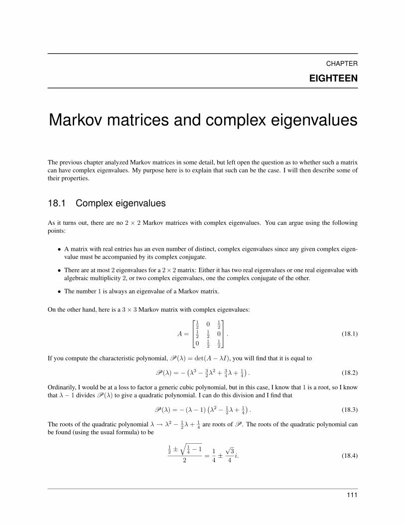
CHAPTER

EIGHTEEN

Markov matrices and complex eigenvalues

The previous chapter analyzed Markov matrices in some detail, but left open the question as to whether such a matrixcan have complex eigenvalues. My purpose here is to explain that such can be the case. I will then describe some oftheir properties.

18.1 Complex eigenvalues

As it turns out, there are no 2 × 2 Markov matrices with complex eigenvalues. You can argue using the followingpoints:

• A matrix with real entries has an even number of distinct, complex eigenvalues since any given complex eigen-value must be accompanied by its complex conjugate.

• There are at most 2 eigenvalues for a 2× 2 matrix: Either it has two real eigenvalues or one real eigenvalue withalgebraic multiplicity 2, or two complex eigenvalues, one the complex conjugate of the other.

• The number 1 is always an eigenvalue of a Markov matrix.

On the other hand, here is a 3× 3 Markov matrix with complex eigenvalues:

A =

12 0 1

212

12 0

0 12

12

. (18.1)

If you compute the characteristic polynomial, P(λ) = det(A− λI), you will find that it is equal to

P(λ) = −(λ3 − 3

2λ2 + 3

4λ+ 14

). (18.2)

Ordinarily, I would be at a loss to factor a generic cubic polynomial, but in this case, I know that 1 is a root, so I knowthat λ− 1 divides P(λ) to give a quadratic polynomial. I can do this division and I find that

P(λ) = − (λ− 1)(λ2 − 1

2λ+ 14

). (18.3)

The roots of the quadratic polynomial λ → λ2 − 12λ + 1

4 are roots of P . The roots of the quadratic polynomial canbe found (using the usual formula) to be

12 ±

√14 − 1

2=

14±√

34i. (18.4)

111

You might complain that the matrix A here has some entries equal zero, and it would be more impressive to see anexample where all entries of A are positive. If this is your attitude, then consider the Markov matrix

A =

12

116

716

716

12

116

116

716

12

(18.5)

whose characteristic polynomial is −(λ3 − 3

2λ2 + 171

256λ−43256

). The roots of the latter are 1 and 1

4 ±3√

316 i.

18.2 The size of the complex eigenvalues

I demonstrated in the previous chapter that a Markov matrix with no zero entries has a single real eigenvalue equalto 1 and that all of its remaining real eigenvalues have absolute value less than 1. An argument very much along thesame lines will demonstrate that the absolute value of any complex eigenvalue of such a matrix is less than 1 also. For

example, the absolute value of the complex eigenvalues for the matrix in (18.5) is√

3164 .

To see how this works in the general case, let’s again use A to denote our Markov matrix with all Ajk > 0. If λ isa complex eigenvalue for A, then it must be a complex eigenvalue for AT . Let ~v denote a corresponding complexeigenvector; thus AT~v = λ~v. In terms of components, this says that

A1kv1 +A2kv2 + · · ·+Ankvn = λvk (18.6)

for any k ∈ {1, 2, . . . , n}. Taking absolute values of both sides in (18.6) finds the inequality

A1k|v1|+A2k|v2|+ · · ·+Ank|vn| ≥ |λ||vk| (18.7)

Here, I have used two facts about absolute values: First, the absolute value of λvk is the product of |λ| and |vk|. Indeed,if a and b are any two complex numbers, then |ab| = |a| |b| which you can see by writing both a and b in polar form.Thus, write a = reiθ and b = seiϕ with s and r non-negative. Then ab = rsei(θ+ϕ) and so the absolute value of ab isrs which is also |a| |b|. Meanwhile, I used the fact that |a+ b| ≤ |a|+ |b| in an iterated fashion to obtain

|A1kv1 +A2kv2 + · · ·+Ankvn| ≤ A1k|v1|+ |A2kv2 + · · ·+Ankvn| (18.8)≤ A1k|v1|+A2k|v2|+ |A3kv3 + · · ·+Ankvn|...≤ A1k|v1|+A2k|v2|+ · · ·+Ank|vn|.

to deduce that the expression on the left side of (18.7) is no less than that on the right side. By the way, the fact that|a + b| ≤ |a| + |b| holds for complex numbers is another way to say that the sum of the lengths of any two sides to atriangle is no less than the length of the third side.

Consider the inequality depicted in (18.7) in the case that k is chosen so that

|vk| ≥ |vj | for all j ∈ {1, . . . , n}. (18.9)

Thus, vk has the largest absolute value of any entry of ~v. In this case, each |vj | that appears on the left side of (18.7) isno larger than |vk|, so the left-hand side is even larger if each |vj | is replaced by |vk|. This done, then (18.7) finds that

(A1k +A2k + · · ·+Ank)|vk| ≥ |λ||vk|, (18.10)

Since A1k +A2k + · · ·+Ank = 1, this last expression finds that |vk| ≥ |λ| |vk| and so 1 ≥ |λ|.

Now, to see that |λ| is actually less than 1, let us see what is required if every one of the inequalities that were used togo from (18.6) to (18.7) and from (18.7) to (18.10) are equalities. Indeed, if any one them is a strict inequality, then1 > |λ| is the result. Let’s work this task backwards: To go from (18.7) to (18.10) with equality requires that each

112 Chapter 18. Markov matrices and complex eigenvalues

vj have the same norm as vk. To go from (18.6) to (18.7), we used the triangle inequality roughly n times, this theassertion that |a + b| ≤ |a|+ |b| for any two complex numbers a and b. Now this is an equality if and only if a = rbwith r > 0; thus if and only if the triangle is degenerated to one where the a+ b edge contains both the a and b edgesas segments.

In the cases at hand, this means that Ajkvj = rAkkvk for each j. Thus, not only does each vj have the same norm asvk, each is a multiple of vk with that multiple being a positive real number. This means that the multiple is 1. Thus,the vector is a multiple of the vector whose entries are all equal to 1. As we saw in Handout 14, this last vector is aneigenvector of A with eigenvalue 1 so if |λ| = 1, then λ = 1 and so isn’t complex.

18.3 Another Markov chain example

The term Markov chain refers to an unending sequence, {~p(0), ~p(1), ~p(2), . . . } of vectors that are obtained from ~p(0)by successive applications of a Markov matrix A. Thus,

~p(t) = A~p(t− 1) and so ~p(t) = At~p(0). (18.11)

I gave an example from genetics of such a Markov chain in Chapter 15. What follows is a hypothetical example frombiochemistry.

There is a molecule that is much like DNA that plays a fundamental role in cell biology, this denoted by RNA.Whereas DNA is composed of two strands intertwined as a double helix, a typical RNA molecule has just one longstrand, usually folded in a complicated fashion, that is composed of standard segments linked end to end. As withDNA, each segment can be one of four kinds, the ones that occur in RNA are denoted as G, C, A and U. There aremyriad cellular roles for RNA and the study of these is arguably one of the hottest items these days in cell biology.In any event, imagine that as you are analyzing the constituent molecules in a cell, you come across a long strand ofRNA and wonder if the sequence of segments, say AGACUA· · · , is “random” or not.

To study this question, you should know that a typical RNA strand is constructed by sequentially adding segmentsfrom one end. Your talented biochemist friend has done some experiments and determined that in a test tube (in vitro,as they say), the probability of using one of A, G, C, or U for the tth segment depends on which of A, C, G or U hasbeen used for the (t−1)st segment. This is to say that if we label A as 1, G as 2, C as 3 and U as 4, then the probability,pj(t) of seeing the segment of the kind labeled j ∈ {1, 2, 3, 4} in the tth segment is given by

pj(t) = Aj1p1(t− 1) +Aj2p2(t− 1) +Aj3p3(t− 1) +Aj4p4(t− 1) (18.12)

whereAjk denotes the conditional probability of a given segment being of the kind labeled by j if the previous segmentis of the kind labeled by k. For example, if your biochemist friend finds no bias toward one or the other base, then onewould expect that each Ajk has value 1

4 . In any event, A is a Markov matrix, and if we introduce ~p(t) ∈ R4 to denotethe vector whose kth entry is pk(t), then the equation in (18.12) has the form of (18.11).

Now, those of you with some biochemistry experience might argue that to analyze the molecules that comprise a cell,it is rather difficult to extract them without breakage. Thus, if you find a strand of RNA, you may not be seeing thewhole strand from start to finish and so the segment that you are labeling as t = 0 may not have been the startingsegment when the strand was made in the cell. Having said this, you would then question the utility of the ‘solution’,~p(t) = At~p(0) since there is no way to know ~p(0) if the strand has been broken. Moreover, there is no way to see ifthe strand was broken.

As it turns out, this objection is a red herring of sorts because one of the virtues of a Markov chain is that the formof ~p(t) is determined solely by ~p(t− 1). This has the following pleasant consequence: Whether our starting segmentis the original t = 0 segment, or some t = N > 0 segment makes no difference if we are looking at the subsequentsegments. To see why, let us suppose that the strand was broken at segment N and that what we are calling strand twas originally strand t + N . Not knowing the strand was broken, our equation reads ~p(t) = At~p(0). Knowing thestrand was broken, we must relabel and equate our original ~p(t) with the vector ~p(t + N) that is obtained from thestarting vector, ~p(0), of the unbroken strand by the equation ~p(t+N) = At+N~p(0).

18.3. Another Markov chain example 113

Even though our equation ~p(t) = At~p(0) has the tth power of A while the equation ~p(t + N) = At+N~p(0) has the(t+N)th power, these two equations make the identical predictions. To see that such is the case, note that the equationfor ~p(t+N) can just as well be written as ~p(t+N) = At~p(N) since ~p(N) = AN~p(0).

18.4 The behavior of a Markov chain as t→∞

Suppose that we have a Markov chain whose matrix A has all entries positive and has a basis of eigenvectors. In thisregard, we can allow complex eigenvectors. Let us use ~e1 to denote the one eigenvector whose eigenvalue is 1, and let{~e2, . . . , ~en} denote the others. We can then write our starting ~p(0) as

~p(0) = ~e1 +n∑k=2

ck~ek (18.13)

where ck is real if ~ek has a real eigenvalue, but complex when ~ek has a complex eigenvalue. With regards to the lattercase, since our vector ~p(0) is real, the coefficients ck and ck′ must be complex conjugates of each other when thecorresponding ~ek and ~ek′ are complex conjugates also.

I need to explain why ~e1 has the factor 1 in front. This requires a bit of a digression: As you may recall from theprevious chapter, the vector ~e1 can be assumed to have purely positive entries that sum to 1. I am assuming that suchis the case. I also argued that the entries of any eigenvector with real eigenvalue less than 1 must sum to zero. Thismust also be the case for any eigenvector with complex eigenvalue. Indeed, to see why, suppose that ~ek has eigenvalueλ 6= 1, either real or complex. Let ~v denote the vector whose entries all equal 1. Thus, ~v is the eigenvector of AT

with eigenvalue 1. Note that the dot product of ~v with any other vector is the sum of the other vector’s entries. Keepthis last point in mind. Now, consider that the dot product of ~v with A~ek is, on the one hand, λ~v · ~ek, and on the other(AT~v) · ~ek. As AT~v = ~v, we see that λ~v · ~ek = ~v · ~ek and so if λ 6= 1, then ~v · ~ek = 0 and so the sum of the entries ofis zero.

Now, to return to the factor of 1 in front of ~e1, remember that ~p(0) is a vector whose components are probabilities, andso they must sum to 1. Since the components of the vectors ~e2, . . . , ~en sum to zero, this constraint on the sum requiresthe factor 1 in front of ~e1 in (18.13).

With (18.13) in hand, it then follows that any given t > 0 version of ~p(t) is given by

~p(t) = ~e1 +n∑k=2

ckλtk~ek. (18.14)

Since |λt| = |λ|t and each λ that appears in (18.14) has absolute value less than 1, we see that the large t versions of~p(t) are very close to ~e1. This is to say that

limt→∞

~p(t) = ~e1. (18.15)

This last fact demonstrates that as t increases along a Markov chain, there is less and less memory of the starting vector~p(0). It is sort of like the aging process in humans: As t→∞, a Markov chain approaches a state of complete senility,a state with no memory of the past.

18.5 Exercises:

1. Any 2× 2 Markov matrix has the generic form[

a 1− b1− a b

], where a, b ∈ [0, 1]. Compute the characteristic

polynomial of such a matrix and find expressions for its roots in terms of a and b. In doing so, you will verifythat it has only real roots.

2. Let A denote the matrix in (18.1). Find the eigenvectors for A and compute ~p(1), ~p(2) and limt→∞

~p(t) in the case

that ~p(t) = A~p(t− 1) and ~p(0) =

100

. Finally, write ~p(0) as a linear combination of the eigenvectors for A.

114 Chapter 18. Markov matrices and complex eigenvalues

3. Repeat Problem 2 using for A the matrix in (18.5).

18.5. Exercises 115

CHAPTER

NINETEEN

Symmetric matrices and data sets

Suppose that you take some large number of measurements of various facets of a system that you are studying. Lets saythat there are n facets and you take N � n measurements under different conditions; thus, you generate a collectionof N vectors in Rn which you can label as {~x1, ~x2, . . . , ~xN}.

An issue now is whether some of the n facets that you measure are dependent on the rest. For example, supposethat one facet is the temperature of the sample, and if all of the other facets of the system are completely determinedby the temperature, then all of these N vectors will lie on very near some curve in the n-dimensional space, a curveparameterized as T → ~x(T ) by the temperature. On the other hand, if no facets are determined by any collection ofthe others, then the N vectors could be spread in a more or less random fashion through a region of Rn. The pointhere is that if you are interested in discovering relations between the various facets, then you would like to know if thedistribution of theN vectors is spread out or concentrated near some lower dimensional object – a curve or a surface orsome such. Any such concentration towards something less spread out indicates relations between the various facets.

For example, suppose n = 2. If you plot the endpoints of the vectors {~xk} in R2 and see the result as very muchlying near a particular curve (not necessarily a line), this says that the two facets are not able to vary in an independentfashion. Indeed, if y = f(x) is the equation for the curve, it says that the variation in x determines the variation in y.Now, for this n = 2 case, you can go and plot your N vectors and just look at the picture. However, for n > 2, this isgoing to be hard to do. How then can you discern relationships when n > 2?

19.1 An example from biology

Here is a topical example: The technology is such that it is possible to monitor the levels of huge numbers of proteinsin a cell as it goes about its business. These proteins are typically interacting with each other, and so it is of crucialimport to determine which are influencing which. Let n denote the number of proteins involved. Discerning the levelsof these n proteins at some N times during the cell cycle with various environmental factors altered at various timesgives some very large data set of the sort described above, N vectors in Rn. Of interest is how these vectors distributethemselves – is it random through some region, or are the vectors concentrated near some intrinsically much thinnerset such as a curve, surface or what ever in Rn. If the latter is the case, then the structure of this thinner set, a curve, asurface or whatever, carries information about the complicated chemical interactions in a cell.

19.2 A fundamental concern

I don’t think that there is a completely foolproof way to discern relationships between a bunch of vectors in Rn. Whatfollows is an n = 2 example to keep in mind. As is typically the case, the vectors {~xk} can not be too big; theyare constrained to lie in some region of fixed size in Rn. Let me suppose in this example that no vector from thiscollection has norm greater than 1 and so all lie in the disk of radius 1 about the origin.

116

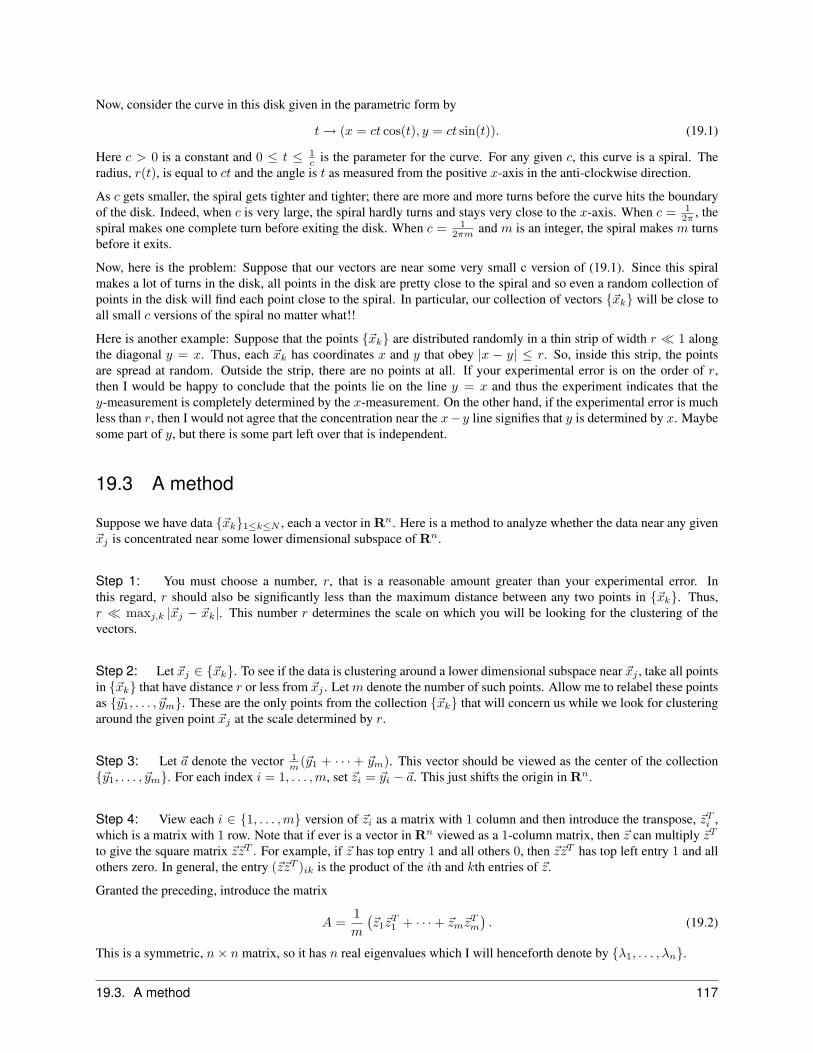
Now, consider the curve in this disk given in the parametric form by

t→ (x = ct cos(t), y = ct sin(t)). (19.1)

Here c > 0 is a constant and 0 ≤ t ≤ 1c is the parameter for the curve. For any given c, this curve is a spiral. The

radius, r(t), is equal to ct and the angle is t as measured from the positive x-axis in the anti-clockwise direction.

As c gets smaller, the spiral gets tighter and tighter; there are more and more turns before the curve hits the boundaryof the disk. Indeed, when c is very large, the spiral hardly turns and stays very close to the x-axis. When c = 1

2π , thespiral makes one complete turn before exiting the disk. When c = 1

2πm and m is an integer, the spiral makes m turnsbefore it exits.

Now, here is the problem: Suppose that our vectors are near some very small c version of (19.1). Since this spiralmakes a lot of turns in the disk, all points in the disk are pretty close to the spiral and so even a random collection ofpoints in the disk will find each point close to the spiral. In particular, our collection of vectors {~xk} will be close toall small c versions of the spiral no matter what!!

Here is another example: Suppose that the points {~xk} are distributed randomly in a thin strip of width r � 1 alongthe diagonal y = x. Thus, each ~xk has coordinates x and y that obey |x − y| ≤ r. So, inside this strip, the pointsare spread at random. Outside the strip, there are no points at all. If your experimental error is on the order of r,then I would be happy to conclude that the points lie on the line y = x and thus the experiment indicates that they-measurement is completely determined by the x-measurement. On the other hand, if the experimental error is muchless than r, then I would not agree that the concentration near the x− y line signifies that y is determined by x. Maybesome part of y, but there is some part left over that is independent.

19.3 A method

Suppose we have data {~xk}1≤k≤N , each a vector in Rn. Here is a method to analyze whether the data near any given~xj is concentrated near some lower dimensional subspace of Rn.

Step 1: You must choose a number, r, that is a reasonable amount greater than your experimental error. Inthis regard, r should also be significantly less than the maximum distance between any two points in {~xk}. Thus,r � maxj,k |~xj − ~xk|. This number r determines the scale on which you will be looking for the clustering of thevectors.

Step 2: Let ~xj ∈ {~xk}. To see if the data is clustering around a lower dimensional subspace near ~xj , take all pointsin {~xk} that have distance r or less from ~xj . Letm denote the number of such points. Allow me to relabel these pointsas {~y1, . . . , ~ym}. These are the only points from the collection {~xk} that will concern us while we look for clusteringaround the given point ~xj at the scale determined by r.

Step 3: Let ~a denote the vector 1m (~y1 + · · · + ~ym). This vector should be viewed as the center of the collection

{~y1, . . . , ~ym}. For each index i = 1, . . . ,m, set ~zi = ~yi − ~a. This just shifts the origin in Rn.

Step 4: View each i ∈ {1, . . . ,m} version of ~zi as a matrix with 1 column and then introduce the transpose, ~zTi ,which is a matrix with 1 row. Note that if ever is a vector in Rn viewed as a 1-column matrix, then ~z can multiply ~zT

to give the square matrix ~z~zT . For example, if ~z has top entry 1 and all others 0, then ~z~zT has top left entry 1 and allothers zero. In general, the entry (~z~zT )ik is the product of the ith and kth entries of ~z.

Granted the preceding, introduce the matrix

A =1m

(~z1~z

T1 + · · ·+ ~zm~z

Tm

). (19.2)

This is a symmetric, n× n matrix, so it has n real eigenvalues which I will henceforth denote by {λ1, . . . , λn}.

19.3. A method 117

Step 5: As I explain below, none of the eigenvalues has absolute value greater than r2. I also explain below why Ahas no negative eigenvalues. Granted this, then A’s eigenvalues can be anywhere from 0 to r2. Those eigenvalues thatare much smaller than r2 correspond to ‘pinched’ directions. If n − d ≤ n of the eigenvalues are much smaller thanr2, this indicates that the distribution of the vectors from {~xk} with distance r or less from ~xj is concentrated near asubspace of Rn whose dimension is d. To quantify this, I am going to say that the vectors near ~xj cluster around asubspace whose dimension is no greater than d when A has n− d or more eigenvalues that are smaller than 1

2(n+2)r2.

In this regard, note that I am not going to expect much accuracy with this prediction unless m is large.

I give some examples below to illustrate what is going on. At the end, I outline my reasons for choosing the factor1

2(n+2) to distinguish between small and reasonably sized eigenvalues.

19.4 Some loose ends

To tie up some loose ends, let me show you why all of A’s eigenvalues are in the interval between 0 and r2. To thisend, suppose that ~v is some vector. To see what A~v looks like, the first thing to realize is that if ~z is any given vector,then ~zT~v is a 1× 1 matrix, thus a number and that this number is the dot product between ~z and ~v. This implies that

A~v =1m

(~z1 · ~v)~z1 + · · ·+ 1m

(~zm · ~v)~zm. (19.3)

Therefore, if I take the dot product of A~v with ~v, I find that

~v · (A~v) =1m

(~z1 · ~v)2 + · · ·+ 1m

(~zm · ~v)2. (19.4)

Note that this is a sum of non-negative terms, so ~v · (A~v) ≥ 0 for any vector ~v.

Now suppose that ~v is an eigenvector with eigenvalue λ. Then A~v = λ~v and so ~v · (A~v) = λ|~v|2. As this isnon-negative, we see that λ ≥ 0.

To see that λ ≤ r2, use the fact that|~z · ~v| ≤ |~z| |~v| (19.5)

for any given vector on each term on the right hand side of (19.5) to conclude that

~v · (A~v) ≤ 1m|~z1|2 |~v|2 + · · ·+ 1

m|~zm|2 |~v|2. (19.6)

When I pull out the common factor 1m |~v|

2 on the right of this last inequality, I find that

~v · (A~v) ≤ 1m

(|~z1|2 + · · ·+ |~zm|2

)|~v|2 (19.7)

since each ~zk has norm less than r, the right-hand side of (19.7) is no larger than r2|~v|2. Thus,

~v · (A~v) ≤ r2|~v|2 (19.8)

for any vector ~v.

Now, if ~v is an eigenvector with eigenvalue λ, then the left-hand side of this last equation is λ|~v|2 and so λ ≤ r2 asclaimed.

19.5 Some examples

What follows are a few examples to try to convince you that my attempt at estimating a dimension is not unreasonable..

118 Chapter 19. Symmetric matrices and data sets

Example 1: Suppose that all ~zk sit very close to the origin, for example, suppose that each ~zk has |~zk| < εr withε2 ≤ 1

2(n+2) . To see what this implies, return now to (19.7) to conclude that

~v · (A~v) ≤ ε2r2|~v|2. (19.9)

This then means A’s eigenvalues are no larger than ε2r2 which is smaller than 12(n+2)r

2. Thus, we would predict thevectors from {~xk} are clustering around a point near ~xj .

Example 2: Suppose that m is large and that the vectors {~xk} all sit on a single line, and that they are evenlydistributed along the line. In particular, let ~z denote the unit tangent vector to the line, and suppose that ~zk = (−1 +

2km+1 )r~z. Thus, ~z1 = −m−1

m+1r~z and ~zm = m−1m+1r~z. This being the case

A =r2

m

m∑k=1

(−1 + 2k

m+1

)2

~z~zT . (19.10)

As it turns out, this sum can be computed in closed form and the result is

A =r2

3m− 1m+ 1

~z~zT . (19.11)

The matrix A has the form c~z~zT where c is a constant. Now any matrix A = c~z~zT has the following property: If ~v isany vector in Rn, then

A~v = c~z (~z · ~v) . (19.12)

Thus, A~v = 0 if ~v is orthogonal to ~z, and A~z = c~z. Hence A has 0 and c as its eigenvalues, where 0 has multiplicityn− 1 and c has multiplicity 1.

In our case, this means that there is one eigenvalue that is on the order of r2

3 and the others are all zero. Thus, wewould say that the clustering here is towards a subspace of dimension 1, and this is precisely the case.

Example 3: To generalize the preceding example, suppose that d ≥ 1, that V ⊂ Rn is a d-dimensional subspace,and that the vectors {~zk}1≤k≤m all lie in V .

In this case, one can immediately deduce thatA will have n−d orthonormal eigenvectors that have zero as eigenvalue.Indeed, any vector in the orthogonal complement to V is in the kernel of A and so has zero eigenvalue. As thisorthogonal subspace has dimension n− d, so A has n− d linearly independent eigenvalues with eigenvalue 0.

Thus, we see predict here that the clustering is towards a subspace whose dimension is no greater than d.

19.6 Small versus reasonably sized eigenvalues

I am going to give some indication here for my choice of the factor 12(n−d+2) to distinguish the small eigenvalue of

A. Note here that you or others might want some other, smaller factor. For example, I am probably being conservativewith this factor.

To explain where this factor 12(n+2) is coming from, I have to take you on a digression that starts here with the

introduction of the uniform probability function on the ball of radius r in Rd. This is to say that the probability ofchoosing a point in any given subset of the ball is proportional to the d-dimensional volume of the subset. To eachvector ~u, in this ball (thus, to each ~u with |~u| ≤ r), we can assign the square matrix ~u~uT . This can be viewed as arandom variable that maps vectors in the ball to d× d matrices. For example, in the case d = 2, one has

~u~uT =[x2 xyxy y2

]. (19.13)

19.6. Small versus reasonably sized eigenvalues 119

For any d, the mean of the random variable ~u → ~u~uT is the matrix whose entry in the jth row and kth column is theaverage of ujuk over the ball. These averages can be computed and one finds that the mean of ~u~uT is r2

d+2Id, whereId is the d× d identity matrix.

Keeping all of this in mind, go back to the formula for A in (19.2). Suppose that I consider a set of m vectors,{~uk}1≤k≤m that all lie in a d-dimensional subspace. Suppose further that I sprinkle these vectors at random in theradius r ball inside this subspace. I can then view

A =1m

(~u1~u

T1 + · · ·+ ~um~u

Tm

)(19.14)

as the average of m identical, but unrelated random variables, this being m maps of the form ~u → ~uT . According tothe Central Limit Theorem, when m is large, the probability that A differs from r2

d+2Id is very small.

If in my actual data, the vectors {~zk}, are truly clustering around a d-dimensional subspace of Rn and are more orless randomly sprinkled in the radius r ball of this set, then I should expect the following:

When m is very large, the Central Limit Theorem tells me that the matrix A in (19.2) is very close to thematrix r2

d+2P , where P here denotes the orthogonal projection on to the subspace in question.

Thus, it should have d eigenvalues that are very close to r2

d+2 and n − d eigenvalues that are much smaller than thisnumber. In particular, when m is large, then under the hypothesis that the vectors {~zk}1≤k≤m are sprinkled at randomin a d-dimensional subspace, the matrix A in (19.2) will be very likely to have d eigenvalues that are on the order ofr2

d+2 and n− d eigenvalues that are zero.

This application of the Central Limit Theorem explains my preference for the size distinction 12(n+2)r

2 between smalleigenvalues of A and eigenvalues that are of reasonable size. I think that this cut-off is rather conservative and one cantake a somewhat larger one.

19.7 Exercises:

1. The purpose of this exercise is to compute the average of the matrix in (19.13) over the disk of radius r in thexy-plane. This average is the matrix, U , whose entries are

U11 =1πr2

∫∫x2 dx dy, U22 =

1πr2

∫∫y2 dx dy, and U12 = U21 =

1πr2

∫∫xy dx dy.

To compute U , change to polar coordinates (ρ, θ) where ρ ≥ 0 and θ ∈ [0, 2π] using the formula x = ρ cos(θ)and y = ρ sin(θ). Show that

(a) U11 = 1πr2

∫ 2π

0

∫ r0ρ2 cos2(θ)ρ dρ dθ,

(b) U22 = 1πr2

∫ 2π

0

∫ r0ρ2 sin2(θ)ρ dρ dθ, and

(c) U12 = U21 = 1πr2

∫ 2π

0

∫ r0ρ2 sin(θ) cos(θ)ρ dρ dθ.

Next, use the formula cos(2θ) = 2 cos2(θ) − 1 = 1 − 2 sin2(θ) and sin(2θ) = 2 sin(θ) cos(θ) to do the angleintegrals first and so find that

(d) U11 = U22 = 1r2

∫ r0ρ3 dρ, and

(e) U12 = U21 = 0.

Finally, do the ρ-integral to find that U11 = U22 = 14r

2 and U12 = U21 = 0. Note that this means that U is thed = 2 version of r2

d+2Id.

120 Chapter 19. Symmetric matrices and data sets

LECTURE NOTES ON PROBABILITY, STATISTICS AND LINEAR...

Documents

Transcript of LECTURE NOTES ON PROBABILITY, STATISTICS AND LINEAR...