1

Lecture notes on locally compact quantum groups

Summer school, Bedlewo, June 28–July 11, 2015

Martijn Caspers

2

Contents

1 Introduction 31.1 What is a good definition of a locally compact quantum group? . . . . . . 31.2 Further literature . . . . . . . . . . . . . . . . . . . . . . . . . . . . . . . . 61.3 Some preliminaries and notation . . . . . . . . . . . . . . . . . . . . . . . 61.4 Acknowledgements . . . . . . . . . . . . . . . . . . . . . . . . . . . . . . . 7

2 Von Neumann algebras 82.1 Von Neumann algebras . . . . . . . . . . . . . . . . . . . . . . . . . . . . . 82.2 Tomita–Takesaki theory . . . . . . . . . . . . . . . . . . . . . . . . . . . . 10

3 Locally compact quantum groups 123.1 The definition . . . . . . . . . . . . . . . . . . . . . . . . . . . . . . . . . . 123.2 Corepresentation theory . . . . . . . . . . . . . . . . . . . . . . . . . . . . 143.3 The antipode and its polar decomposition . . . . . . . . . . . . . . . . . . 153.4 Example: von Neumann algebraic quantum SUq(2) . . . . . . . . . . . . . 15

4 Pontrjagin duality 174.1 The left multiplicative unitary . . . . . . . . . . . . . . . . . . . . . . . . . 174.2 The dual quantum group: the von Neumann algebra and comultiplication 184.3 Dual Haar weights . . . . . . . . . . . . . . . . . . . . . . . . . . . . . . . 194.4 Relations between the quantum group and its dual . . . . . . . . . . . . . 21

5 Examples 235.1 SUq(1, 1) on the Hopf ∗-algebra level . . . . . . . . . . . . . . . . . . . . . 245.2 Special functions related to the multiplicative unitary . . . . . . . . . . . 275.3 The GNS-construction for the Haar weight . . . . . . . . . . . . . . . . . 315.4 The multiplicative unitary and the comultiplication . . . . . . . . . . . . . 33

6 Cocycle twisting 346.1 Cocycle twisitng . . . . . . . . . . . . . . . . . . . . . . . . . . . . . . . . 346.2 Twisting by Galois coobjects . . . . . . . . . . . . . . . . . . . . . . . . . 366.3 Concluding remarks about SUq(1, 1) . . . . . . . . . . . . . . . . . . . . . 38

3

1 Introduction

These notes contain an introduction to the theory of locally compact quantum group. Inparticular we focus on the problems/novelties involved in defining such objects comparedto compact quantum groups. It turns out that there are different approaches to thetheory, but here we will mainly focus on the approach taken by J. Kustermans and S.Vaes [22], [23] which was settled successfully around the year 2000 and is nowadays themost applied approach.

These lecture notes are set up in the following way.

• In the Introduction we will cover some background material: what is the propernotion of a non-compact quantum group? What is the history behind their de-velopment? How are operator algebras involved? And in particular, what is theadvantage of a von Neumann-algebraic approach above a C∗-algebraic approachand the other way around. We will also give references and the reader shouldsee these notes as a guideline to start reading in these references, which can betechnically quite demanding.

• In Section 2 we give some background on von Neumann algebras. We assumethat the reader is familiar with some general C∗-algebra theory; essentially whatis needed to treat compact quantum groups. Section 2 serves as a quick reminderof some essential ingredients and notation we need for the further sections.

• In Section 3 we treat the Kustermans–Vaes approach to locally compact quantumgroups. We state their definition and give basic examples.

• Section 4 treats Pontrjagin-duality (or Pontrjagin-Van Kampen duality). Wedefine the left regular representation for quantum groups and show how a dualquantum group can be constructed from it. The construction of the left regularrepresentation can be considered as the most crucial and essential part of thetheory. We also show the relations between the various objects defined so far. Inparticular, we focus on the relations between a quantum group and its dual.

• Section 5 treats examples of locally compact quantum groups. It should imme-diately be said that examples are very sparse and the construction of them is anon-trivial task in itself.

• Section 6 gives a very brief treatment of cocycle twisting. The section is certainlya bit too much on the concise side, as for a suitable treatment we should haveintroduced crossed products first.

1.1 What is a good definition of a locally compact quantum group?

Recall that if G is a locally compact abelian group, then the dual group G is definedas the group of all irreducible unitary strongly continuous representations of G. Since

4

irreducible representations are necessarily one dimensional (as G is abelian) we can mul-tiply representations as functions and hence G carries a group structure. The Pontrjagin

duality theorem states thatG is isomorphic as a group to G.

One of the main motivating questions behind the development of operator quantumgroups is if the Pontrjagin duality theorem can be extended beyond the category ofabelian groups. That is, one searches for a category in which the objects incorporate atleast all locally compact groups. But since for an arbitrary locally compact group theirreducible representations are not necessarily 1-dimensional anymore it is not expectedthat the dual will have the structure of a group anymore. That is, the category we arelooking for will include more objects (in particular it turns out that group von Neumannalgebras will be in there).

The other motivating question is that in the 1980’s work of V. Drinfeld and S.L.Woronowicz produced examples of structures admitting nice representation theory. Thetypical examples are SUq(n) and its corresponding q-deformed universal enveloping Liealgebra. The former one is due to Woronowicz, the latter one due to Drinfeld. Theseturn out to give examples of compact quantum groups (see the other mini-courses ofthis summer school). But also – on a purely algebraic level – notions of SUq(n,m) havebeen found. These give certain series of examples that should somehow be part of aconceptual category that we would like to call locally compact quantum groups.

Summarizing the previous paragraphs a good notion of a locally compact quantumgroup should at least:

• Feature a Pontrjagin duality theorem;

• Incorporate all compact quantum groups;

• Incorporate all locally compact groups;

• Incorporate known q-deformed examples of (non-compact) Lie groups;

• Be a concise and workable definition.

So which approach we take? In 1987 Woronowicz suitably settled the theory ofcompact quantum groups [36]. We recall his definition here:

Definition 1.1. A compact quantum group consists of a pair (A,∆) where A is a unitalC∗-algebra and ∆ : A → A ⊗ A is a unital ∗-homomorphism such that (∆ ⊗ ι) ∆ =(ι⊗∆) ∆. Moreover, the cancellation laws hold:

∆(A)(A⊗ 1) = A⊗ A = ∆(A)(1⊗ A).

Here the tensor product is the minimal tensor product of C∗-algebras and the overlineindicates the norm closure.

5

These conditions are sufficient to derive the existence of a Haar weight on the quan-tum group. It turns out that simply generalizing this definition to a ‘non-compact’definition is insufficient. Such a generalization would mean that we drop the unital-ity condition on A and let ∆ be a map from A to M(A ⊗ A); the multiplier algebra ofA⊗A. The classical case would then correspond to A = C0(G). Unfortunately there is no(known) reasonable set of extra assumptions on A that allows us to derive the existenceof the Haar weight(s) in this case.

Another approach to the theory (mainly due to Baaj–Skandalis and Woronowiczfrom the 1990’s) is through multiplicative unitaries. Roughly, for classical groups thisapproach postulates the existence of the left regular representation. The approach ispartly successful, also nowadays (see for example [25]), but again proving the existenceof Haar weights with a reasonable set of extra assumptions has not been possible. Thereader interested in this approach is referred to [30] and references there. In the currentnotes multiplicative unitaries will be part of our theory as we shall be able to constructthem.

So what else can we do? We approach the theory by postulating the existence ofHaar weights. There is one drawback to this approach: namely that the Haar weightsare postulated to exist whereas in the case of locally compact groups one is able toconstruct them. There are many advantages though: namely one can define locallycompact quantum groups in a way that satisfies all of the bullet points above. Moreover,in examples the Haar weights are usually easy to construct. Or better: they are easy tofind, as they are unique up to scaling.

We state the precise definition of a locally compact quantum group in Section 3. Thisdefinition is proposed by Johan Kustermans and Stefaan Vaes as they have successfullyestablished this approach in [22], [23]. The Kustermans–Vaes theory of locally compactquantum groups comes in two versions: a von Neumann algebraic one (the measurableside) and a C∗-algebraic one (the continuous side). The original paper [22] is written inthe C∗-algebraic language but uses von Neumann algebraic techniques in the proofs. Apurely von Neumann algebraic definition is given in [23] but the proofs rely on [22]. Aself-contained approach to the Von Neumann algebraic theory was later also given byVan Daele [35].

The main importance of the von Neumann algebraic approach is that one is able touse Tomita-Takesaki theory. We do not expect that the reader is familiar with Tomita-Takesaki theory, but let us say some words about it. An integral on a matrix algebra isas a mapping ϕ : Mn(C)+ → [0,∞] that preserves convex combinations. The integralis called a trace if ϕ(xy) = ϕ(yx). It turns out that in many application this traceproperty is of extreme importance. So what if ϕ is not a trace? Well, then there isstill a way to suitably treat this theory: Tomita-Takesaki theory. There exists a one–parameter series of automorphisms σ : R → Aut(Mn(C)) such that we have the skewrelation ϕ(xy) = ϕ(yσ−i(x)), where σ−i is an analytic extension of t 7→ σt. This isa (main) consequence of Tomita-Takesaki theory and it is remarkably effective for vonNeumann algebra theory. In fact classification of hyperfinite von Neumann algebras

6

can fully be described in terms of such automorphism groups. There is no general C∗-algebraic version of such theory (it in fact becomes a new definition, which you mightencounter as KMS-state) and this is what makes von Neumann algebras important inthe theory of quantum groups.

So what about C∗-algebras? Operator algebraic quantum groups need C∗-algebrasbecause of their representation theory. They should not be regarded as an alternativeapproach to the theory, but they go side-by-side with the von Neumann algebraic theory.They enhance the von Neumann algebraic theory and vice-versa. A beautiful exampleof this is Kasprzak’s approach to quantum homogeneous spaces [18]. Also, classicallythe representations of a group G correspond to representations of its universal groupC∗-algebra. In quantum group theory, this approach goes completely parallel and wasdeveloped by Kustermans [24].

Finally, does the definition of locally compact quantum groups – being more general– make the definition of compact quantum groups redundant? The answer is definitelyno. In almost any research paper dealing only with the compact case, the compactdefinition is used. The reason is (in my opinion/understanding) that this definition ismore comprehensible (C∗-algebras are accessible to a larger audience) and it is for suremore authentical.

1.2 Further literature

In these notes we introduce the basic concepts of the theory of locally compact quantumgroups and omit almost all technical details. We focus on constructions instead of proofs,giving the reader a good starting point to look further in the literature. In particular,we explain how the Pontrjagin dual quantum groups is constructed as well as manyother features as the antipode, its polar decomposition and the basic treatment of someexamples.

Entering the complete theory requires certainly some time and a basic acquintancewith C∗- and von Neumann algebra theory, but there are good sources available. Ac-cessible references are Stefaan Vaes his thesis [33] and Alfons van Daele his paper [35].These contain a concise and well-explained treatment of general locally compact quan-tum groups. Then there are the original papers [22] and [23] of which [22] contains all theessential proofs. The book [30] also contains a treatment of operator algebraic quantumgroups, but for proofs refers again to [22].

Finally, each of these references require a reasonable background in weight theory forvon Neumann algebras and in particular Tomita-Takesaki theory. For these we refer thereader to the final section of [26] and of course the standard reference [28].

1.3 Some preliminaries and notation

Basic notation. We will basically take over notation from [28]. The symbol ⊗ meansseveral different things: it is an algebraic tensor product of two elements. For C∗-algebras

7

it is the minimal tensor product (see [27]), for von Neumann algebras it is is the closurein the strong operator topology of the algebraic tensor product (which is the usual vonNeumann algebraic tensor product). The symbol ι denotes the identity mapping.

Slicing and tensoring linear maps. If A and B are C∗-algebras (resp. von Neumannalgebras) and π : A → A is a (resp. normal) ∗-homomorphism, then there is a unique(resp. normal) ∗-homomorphism (π⊗ ι) : A⊗B→ A⊗B that maps the algebraic tensorproduct a⊗ b to π(a)⊗ b. Similarly, if ω : A→ C is a bounded (resp. normal) functionalthen there exists a bounded (resp. normal) map (ω ⊗ ι) : A ⊗ B → B sending a ⊗ b toω(a)b.

1.4 Acknowledgements

The author wishes to thank Uwe Franz, Adam Skalski and Piotr Soltan for the invitationto give lectures at their winter school.

Section 7 of the current notes is almost entirely taken from earlier lecture noteswritten together with Erik Koelink for a winter school in Bizerte, 2010 [4]. The authoris indebted to Erik Koelink for allowing him to copy these notes. These results arepublished in [19] (see also [16]).

8

2 Von Neumann algebras

In this section we recall some notions from von Neumann algebra theory. We shall alsobriefly say something about Tomita-Takesaki theory which is important in the theoryof locally compact quantum groups (in fact already for compact quantum groups, it isan important tool). We assume that the reader is familiar with notions from C∗-algebratheory such as the definition of C∗-algebras, GNS-constructions and the Gelfand-Naimarktheorem.

2.1 Von Neumann algebras

Von Neumann algebras are special kinds of C∗-algebras and by definition they are repre-sented as bounded operators on a Hilbert space. In order to define them more precisely,recall that the strong operator topology on B(H) is the topology induced by the semi-norms x 7→ ‖xξ‖, where ξ ∈ H.

Definition 2.1. A von Neumann algebra M is a unital ∗-algebra of bounded operatorson some Hilbert space H that is closed in the strong operator topology.

Von Neumann’s famous double commutant theorem states that a von Neumann al-gebra may alternatively be defined through its double commutant.

Theorem 2.2. Let A ⊆ B(H) be a unital ∗-algebra. A is a von Neumann algebra ifand only if A is equal to its double commutant (A′)′. Here the commutant of an algebraB ⊆ B(H) is defined as

B′ = x ∈ B(H) | ∀y ∈ B : xy = yx.

Example 2.3. Every abelian von Neumann algebra is of the form L∞(X) where X issome measure space. Other examples are L∞(X)⊗B(H) (strong closure of the algebraictensor product) and direct sums of von Neumann algebras. In fact these exhaust allvon Neumann algebras of type I (see [27] for details). Most of the known examples ofnon-compact quantum groups have a type I von Neumann algebra. In particular the vonNeumann algebra of quantum SUq(1, 1) is a type I algebra, see [5].

We let M∗ be the space of all (bounded) functionals M→ C that are continuous forthe strong operator topology on bounded sets. There is a natural pairing,

〈 · , · 〉 : M∗ ×M→ C : (ω, x) 7→ ω(x),

and through this pairing (M∗)∗ = M. Therefore M∗ is called the predual of M. In fact M∗

is the unique (up to isomorphism) Banach space X such that M is the dual of X. Also,a unital C∗-algebra A is a von Neumann algebra if and only if it is the dual of a banachspace X. The topology induced on M by M∗ is called the σ-weak topology (sometimesalso called the ultraweak topology or the σ(M,M∗)-topology).

9

Suppose that (xi)i is a bounded and increasing net of positive elements in M. Thenthere exists a (unique) element x ∈ M+ that is the supremum of (xi)i. That is, ∀i : xi ≤ xand whenever for some y ∈ M+ we have ∀i : xi ≤ y then x ≤ y. We denote supxi for thisx. The following definition should be considered as an unbounded version of a state.

Definition 2.4. A weight ϕ : M+ → [0,∞] is a map that preserves convex combintations.We call a weight ϕ faithful if ϕ(x∗x) = 0 implies that x = 0. A weight ϕ is called normalif ϕ(supxi) = supϕ(xi). Set

nϕ = x ∈ M | ϕ(x∗x) <∞.

The weight ϕ is called semi-finite if the set nϕ is σ-weakly dense in M.

Whereas not every von Neumann algebra possesses a normal, faithful state, everyvon Neumann algebra does posess a normal, faithful semi-finite weight. We shall brieflywrite nsf weight for normal, semi-finite, faithful weight (and this is occassionally doneso in the literature). Now fix a nsf weight ϕ on a von Neumann algebra M. We shall doa GNS-construction as in the C∗-algebra case. Firstly, because of the inequality,

ϕ(x∗y∗yx) ≤ ‖y‖2ϕ(x∗x), x, y ∈ M, (2.1)

we find that nϕ is a left-ideal. Now we equip nϕ with the following inner-product:

〈x, x〉 = ϕ(x∗x), x ∈ nϕ,

which can be extended to an inner product nϕ×nϕ → C through the polarization identity

〈x, y〉 =3∑

k=0

ik〈x+ iky, x+ iky〉, (2.2)

and in fact we shall write as well ϕ(y∗x) for this quantity. So letting mϕ be the linearspan of n∗ϕnϕ we have properly defined ϕ on mϕ. Since ϕ is faithful (2.2) defines anon-degenerate inner-product and we complete nϕ into a Hilbert space Hϕ. We shalldistinguish elements in nϕ viewed as a subset of M from elements in nϕ viewed as anelement of the Hilbert space Hϕ. That is, for x ∈ nϕ ⊆ M we shall write Λϕ(x) for thecorresponding element in Hϕ. So in particular 〈Λϕ(x),Λϕ(y)〉 = ϕ(y∗x). Λϕ turns outto be closed in the σ-weak/norm topology (equivalently in the σ-weak/weak topology).The inequality (2.1) shows that for y ∈ M there is a bounded operator

πϕ(y) : Λϕ(x) 7→ Λϕ(yx).

Using that ϕ is faithful, one can show that the representation πϕ is faithful. Using thatϕ is normal, one can prove that πϕ is continuous in the σ-weak topology. The triple(Hϕ, πϕ,Λϕ) is called the GNS-representation of ϕ (sometimes it is also called the cyclicGNS-representation). Since in these notes ϕ will be fixed (namely the left Haar weight)we will simply write (H, π,Λ).

Remark 2.5. If ϕ is a nsf state, so ϕ(1) = 1. Then Hϕ possesses a cyclic and separatingvector Ωϕ, namely Λϕ(1). In this case it is also common to write Λϕ(x) = xΩϕ.

10

2.2 Tomita–Takesaki theory

Let M be a von Neumann algebra with nsf weight ϕ. We may assume that M is repre-sented on its GNS-space Hϕ for which we shall simply write H. This way we may dropthe GNS-map πϕ in our notation. Consider the anti-linear mapping,

S : Λϕ(x) 7→ Λϕ(x∗), x ∈ nϕ ∩ n∗ϕ.

The mapping is closed and generally unbounded. Let S = J∇1/2 be its polar decom-position. Here J : H → H is an anti-unitary map and ∇1/2 is a closed map withDom(∇1/2) = Dom(S). By Tomita-Takesaki theory:

JMJ = M′, ∇itM∇−it = M, t ∈ R.

In case S and hence ∇ is a bounded operator, the latter fact admits a short proof whichcan be found in [1]. Otherwise the proof is much more involved and can be found in [28].We define the modular automorphism group as:

σϕ : R→ Aut(M) : t 7→(x 7→ ∇itx∇−it

).

We set:

Tϕ = x ∈ M | x is analytic for σϕ and ∀z ∈ C : σϕz (x) ∈ nϕ ∩ n∗ϕ.

The set Tϕ is sometimes referred to as the Tomita algebra, though stricly speaking thisterminology is not correct. It is the Hilbert space identification Λ(Tϕ) that forms aTomita algebra in the sense of [28]. We have the following lemma, of which we includea proof as it involves a standard technique in quantum group theory. Note that in theproof we use that ϕ σϕt = ϕ (which can easily be derived from the definitions) and thatconsequently nϕ is invariant under σϕ.

Lemma 2.6. Tϕ is σ-weakly dense in M.

Proof. Since ϕ is semi-finite, by definition nϕ is dense in M. Since nϕ is a left-ideal we seethat n∗ϕ is a right ideal. It follows that n∗ϕnϕ is contained in n∗ϕ ∩ nϕ. Moreover, we claimthat n∗ϕnϕ is σ-weakly dense in M. Indeed, let (ej)j∈J be a net in nϕ converging σ-weaklyto 1 (which exists by σ-weak density of nϕ in M), then for every x ∈ nϕ the net (e∗jx)j∈Jconverges to x in the σ-weak topology. As nϕ is σ-weakly dense in M, this implies thatn∗ϕnϕ is σ-weakly dense in M. Summarizing we proved that n∗ϕ ∩ nϕ is σ-weakly dense inM. Now take x ∈ n∗ϕ ∩ nϕ. Consider

xn =

√π

n

∫ ∞−∞

e−nt2σϕt (x)dt,

We have xn ∈ Tϕ with σϕz (x) =√

πn

∫∞−∞ e

−n(t−z)2σϕt (x)dt ∈ n∗ϕ ∩ nϕ. Moreover xn → xin the σ-weak topology.

11

Exercise 2.7. Prove that Λ(T 2ϕ ) is dense in Hϕ. Here T 2

ϕ is the product of Tϕ withitself.

Exercise 2.8. Consider the von Neumann algebra M = Mn(C) and let ϕ(x) = Tr(xA)for some positive matrix A ∈Mn(C). Determine J and ∇.

Remark 2.9. The results mentioned in this section are in fact consequences of a biggertheory: Tomita-Takesaki theory (we often mentioned it without really explaing what itis). The complete theory proceeds through the notion of Hilbert algebras and can befound in either [28] or [26]. The general theory is in fact essential in the construction ofthe Haar weights on a (dual) quantum group, but we rather give a reference at a laterpoint than recalling the complete theory here.

12

3 Locally compact quantum groups

In this section we explain the notion of locally compact quantum groups and give classicaland compact examples.

3.1 The definition

The following definition is due to Johan Kustermans and Stefaan Vaes and can be foundin [23]. See also [22].

Definition 3.1. A locally compact quantum group G = (M,∆, ϕ, ψ) is a 4-tuple con-sisting of:

• A von Neumann algebra M;

• A comultiplication ∆ : M → M ⊗M, which is a normal, unital ∗-homomorphismsatisfying the coassociativity relation:

(∆⊗ ι) ∆ = (ι⊗∆) ∆;

• Two normal, semi-finite, faithful weights ϕ : M+ → [0,∞] and ψ : M+ → [0,∞]satisfying:

ϕ((ω ⊗ ι) ∆(x)) = ϕ(x), x ∈ M+, ω ∈ M+∗ ,

ψ((ι⊗ ω) ∆(x)) = ψ(x), x ∈ M+, ω ∈ M+∗ .

(3.1)

Remark 3.2. The weight ϕ in Definition 3.1 is also called the left Haar weight whereasthe weight ψ is called the right Haar weight. It is common to write G = (M,∆) insteadof the 4-tuple (M,∆, ϕ, ψ) and hence suppress the Haar weights in the notation. In factif the Haar weights exist then they must be unique up to multiplication with a positivescalar. The conditions (3.1) are called left invariance (of ϕ) and right invariance (of ψ).Of course these conditions are in the classical case (see Example 3.3) equivalent to theleft and right invariance of the Haar weights on a locally compact group.

Example 3.3. Let G be a locally compact group. Set M = L∞(G) and let ∆G : M →M⊗M be the pull-back of the multiplication. So,

∆G(f)(s, t) = f(st), s, t ∈ G,

which is well-defined as M⊗M ' L∞(G×G). Let ϕ(f) =∫G f(s)ds, f ∈ M+ be integration

against the left Haar measure and let ψ(f) =∫G f(s−1)ds, f ∈ M+ be integration against

the right Haar measure. Then the 4-tuple G = (M,∆G, ϕ, ψ) forms a locally compactquantum group.

Exercise 3.4. Verify that Example 3.3 determines a locally compact quantum group.

13

Example 3.5. Let G be a locally compact group and let

M :=λ(f) | f ∈ L1(G)

′′,

be its group von Neumann algebra. Here λ(f) =∫G f(s)λsds is the left regular represen-

tation, where λs, s ∈ G is acting on L2(G) by means of left translation: (λsξ)(t) = ξ(s−1t)for ξ ∈ L2(G). We have (that is, one can prove that) λs ∈ M, s ∈ G and there exists aunique normal, unital ∗-homomorphism that is determined by,

∆ : M→ M⊗ M : λs 7→ λs ⊗ λs.

For x ∈ M (so in particular it acts on L2(G)) we set ϕ(x∗x) = ‖f‖2L2(G) in case there exists

f ∈ L2(G) such that xg = f ∗ g, g ∈ L2(G). We set ϕ(x∗x) =∞ otherwise. Similarly, forf ∈ G→ C we set f∨(s) = f(s−1)∆−1

G (s). For x ∈ M we set ψ(x∗x) = ‖f∨‖2L2(G) in case

there exists f ∈ L2(G) such that xg = f ∗ g, g ∈ L2(G). We set ψ(x∗x) = ∞ otherwise.The tuple (M, ∆, ϕ, ψ) forms a locally compact quantum group.

Exercise 3.6. Verify that Example 3.5 determines a locally compact quantum group.You may assume that ∆ indeed extends as a normal ∗-homomorphism.

Remark 3.7. Let G be a locally compact abelian group. Let G0 be the set of all stronglycontinuous irreducible unitary representations π : G → B(Hπ) on a Hilbert space Hπ.Two representations π1, π2 ∈ G0 are called unitarily equivalent if there exists a unitarymap U : Hπ1 → Hπ2 intertwining the representations π1 and π2. Let G be the set G0

modulo unitary equivalence. Since irreducible representations of an abelian group are 1-dimensional G carries a multiplication, which is just pointwise multiplication of functionson G. In fact G is a group called the Pontrjagin dual group.

We now relate the Examples 3.3 and 3.5 for abelian groups: we claim that Example3.5 constructed from G is isometrically isomorphic with the locally compact quantumgroup associated with G as constructed in Example 3.3. So let G = (M,∆G, ϕ, ψ) andG = (M, ∆, ϕ, ψ) be locally compact quantum groups constructed in Examples 3.3 and3.5 starting from G. Consider the Fourier transform:

F2 : L2(G)→ L2(G) : f 7→ f ,

where f(π) =∫G f(s)π(s)ds in case f ∈ L1(G) ∩ L2(G). F2 is a unitary transformation.

Furthermore, we get the following spatial identification,

F2MF−12 = L∞(G). (3.2)

In fact under the mapping x 7→ F2xF−12 it turns out that the comultiplication ∆ and

Haar weights ϕ and ψ on M are transfered into the comultiplication ∆G

and left and

right Haar measures on L∞(G).The conclusion is that Example 3.5 should be considered as the Pontrjagin dual quan-

tum group of Example 3.3. We shall come back to Pontjagin duality for arbitrary locally

14

compact quantum groups in Section 4. The discussion above shows that in the abeliancase the identification of the Pontrjagin duals is established by the Fourier transform. Animportant consequence is that Fourier theory for quantum groups partially trivializes,being part of its construction, see [2, Section 5].

Exercise 3.8. Verify that Z and T (the torus) are the Pontrjagin dual group to ea-chother.

Exercise 3.9. Verify (3.2).

Example 3.10. A locally compact quantum group G = (M,∆, ϕ, ψ) is called compactin case ϕ and ψ are states and it is called unimodular in case ϕ = ψ. Compact quan-tum groups are always unimodular. To every compact quantum group in the sense ofDefinition 3.1 there is a canonical way of constructing a compact quantum group in thesense of Woronowicz (see Definition 1.1). Essentially this is done by finding a suitableC∗-subalgebra A of M (being dense in M in the strong operator topology) to which ∆restricts as a comultiplication satisfying the cancellation law. Indeed, one can constructA as follows. We have to jump a bit ahead to Section 4 where the left multiplicative Wwas constructed. Then let A be the norm-closed linear span of all matrix coefficients,

(ι⊗ ω)(W ) | ω ∈ B(L2(G))∗.

One can indeed show that A is a unital C∗-algebra (the argument involves manipulationswith W as in Remark 4.5) which is contained in M. Moreover ∆ restricts to a map A→A⊗ A witnessing that (A,∆) is a compact quantum group in the sense of Woronowicz.

3.2 Corepresentation theory

Representation theory for groups translate into corepresentation theory for locally com-pact quantum groups. A unitary corepresentation of a locally compact quantum groupG is an operator

U ∈ M⊗B(HU ),

satisfying the identity(∆⊗ ι)(U) = U13U23. (3.3)

Example 3.11. If π : G → B(Hπ) is a strongly continuous representation of a lo-cally compact group G on a Hilbert space Hπ, then we may regard π as an element ofL∞(G, B(Hπ)) ' L∞(G) ⊗ B(Hπ). Let Uπ be the element in the latter von Neumannalgebra corresponding to π. Then Uπ is a corepresentation. Indeed, to see this regardUπ again as function on G with values in B(Hπ), so the function s 7→ π(s). Then,(∆⊗ ι)(Uπ) is a two variable function on G with values in B(Hπ), namely (s, t) 7→ π(st),by definition of the comultiplication. Then,

(∆⊗ ι)(Uπ)(s, t) = Uπ(st) = Uπ(s)Uπ(t),

which corresponds to the identity (3.3).

15

If U1 ∈ M ⊗ B(H1) and U2 ∈ M ⊗ B(H2) are corepresentations then we may formthe direct sum corepresentation U1 ⊕ U2 acting on H1 ⊕ H2 by taking the direct sumof the operators. A corepresentation is called irreducible if it cannot be written as thedirect sum of two irreducible operators. A map T : H1 → H2 is called an intertwiner ofU1 and U2 if (1 ⊗ T )U1 = (1 ⊗ T )U2. As for groups, locally compact quantum groupsadmit a Schur lemma: that is U1 is irreducible if and only if the space of intertwiners is1-dimensional.

3.3 The antipode and its polar decomposition

The construction of the anti-pode for locally compact quantum groups is a delicate taskand is done hand-in-hand with the construction of the multiplicative unitary to whichwe come back in Section 4. The following theorem yields the existence of the antipodeand its polar decomposition as a map on the von Neumann algebra. For the details ofits construction we refer to [22] and [35].

Theorem 3.12. We have the following:

1. There exists a unique σ-strongly closed operator S : Dom(S)→ M on a σ-stronglydense domain Dom(S) ⊆ M that has (ι⊗ ω)(W ) | ω ∈ B(L2(G))∗ as a σ-strongcore on which it is determined by:

S(ι⊗ ω)(W ) = (ι⊗ ω)(W ∗).

2. There exists uniquely a ∗-anti-homomorphism R : M→ M and a strongly continu-ous 1-parameter group of automorphisms (τt)t∈R of M such that S = R τ−i/2.

3.4 Example: von Neumann algebraic quantum SUq(2)

Presuming that the example of SUq(2) is treated in one or more of the other mini-courses,we give a quick account of its von Neumann algebraic version. Let −1 < q < 1. Recallthat algebraically SUq(2) is defined as the ∗-algebra generated by operators α and γ thatsatisfy the following relations:

α∗α+ γ∗γ = 1, αα∗ + q2γγ∗ = 1, γγ∗ = γ∗γ, qγα = αγ, qγ∗α = αγ∗.

We shall define an explicit representation for these operators. Set the Hilbert spaceH = L2(N)⊗ L2(Z) with canonical basis en ⊗ fk, n ∈ N, k ∈ Z. And define operators,

αen ⊗ fk =√

1− q2nen−1 ⊗ fk, γen ⊗ fk = qnen ⊗ fk+1.

Let M be the von Neumann algebra generated by α and γ. A (not too hard) exerciseshows that it equals M ' B(L2(N))⊗ L∞(T). The comultiplication is determined by

∆(α) = α⊗ α− qγ∗ ⊗ γ,∆(γ) = γ ⊗ α+ α∗ ⊗ γ,

16

and extends uniquely to a normal, unital ∗-homomorphism ∆ : M→ M⊗M. The Haarweights ϕ = ψ are given by the following formula. Take x = x(t) ∈ L∞(T, B(L2(N)),then:

ϕ(x) =1− q2

2π

∫T

∞∑i=0

q2i〈x(t)ei, ei〉dt.

17

4 Pontrjagin duality

In Remark 3.7 we already explained how duality is involved in the examples we haveseen so far. In this section we construct the Pontrjagin dual of an arbitrary quantumgroup. Pontrjagin duality is one of the main motivations of quantum group theory.The construction of the dual quantum group proceeds via an important operator: themultiplicative unitary.

4.1 The left multiplicative unitary

As observed in Section 3.2 representation theory of groups translates in corepresentationtheory for quantum groups. In particular to any unitary representation π of a groupG on a Hilbert space Hπ one may associated a corepresentation, which is a unitaryoperator Uπ ∈ L∞(G)⊗B(Hπ). See Section 3.2 for details. In case π is the left-regularrepresentation the associated corepresentation Uπ is normally denoted by W and forarbitrary locally compact quantum groups is called the (left) multiplicative unitary. Weshall give its construction for arbitrary compact quantum groups below. It plays themost crucial role in the theory: the single operator W turns out to contain all the dataof G (comultiplication, von Neumann algebra, Haar weights and more) as well as of thedual quantum group G that we shall also construct in this section.

Theorem-Definition 4.1. Let G be a locally compact quantum group. There exists aunique unitary operator W ∈ B(L2(G)⊗ L2(G)) that is determined by:

W ∗ : L2(G)⊗ L2(G)→ L2(G)⊗ L2(G) : Λ(x)⊗ Λ(y) 7→ (Λ⊗ Λ) ∆(y)(x⊗ 1).

Remark 4.1. The proof showing that W in Theorem-Definition 4.1 is isometric relieson the left invariance of the Haar weight ϕ. The more difficult part is to show that W isactually surjective. The proof of this fact relies on the existence of both the left and rightHaar weights of G even though W needs only the left Haar weight to be defined. Werefer to [35] for part of the proof and [22] for the complete proof of Theorem-Definition4.1

Remark 4.2. Let G be a locally compact group. Consider the left regular representationλ : G → B(L2(G)). We may regard λ as an element of L∞(G, B(L2(G))) ' L∞(G) ⊗B(L2(G)). The corresponding element in the latter von Neumann algebra is exactly Wof Theorem–Definition 4.1.

An important feature of W is that it satisfies the pentagon equation:

W12W13W23 = W23W12, (4.1)

which is an equation of operators in B(L2(G) ⊗ L2(G) ⊗ L2(G)). Here we have usedagain the leg-numbering notation W12 = W ⊗ 1,W23 = 1 ⊗W et cetera. We shall nowexplain how W encodes the structure of G := (M,∆, ϕ, ψ). Firstly, we have

M = (id⊗ ω)(W ) | ω ∈ B(L2(G))∗′′.

18

Secondly the comultiplication may be written as

∆(x) = W ∗(1⊗ x)W.

Also the Haar weights can be recovered from W . However, the construction is less directand for the sake of exposition it is better to construct the dual Haar weights instead.

Remark 4.3. The name left multiplicative unitary suggests that there exists also a rightmultiplicative unitary. Indeed such a unitary can be constructed similarly but we willnot do it here.

4.2 The dual quantum group: the von Neumann algebra and comulti-plication

Let G be a locally compact quantum group and let W be its multiplicative unitary. Weshall construct a Pontrjagin dual quantum group G in the following way. Firstly, set

M := (ω ⊗ ι)(W ) | ω ∈ M∗′′ . (4.2)

Remark 4.4. It is not directly clear that Equation (4.2) indeed determines a von Neu-mann algebra: one needs to check that (ω ⊗ ι)(W ) | ω ∈ M∗ is closed under takingadjoints. This follows from the fact that the set defined in (4.4) is dense in M∗.

Next we define a comultiplication ∆ : M→ M⊗ M by setting,

∆(x) = W (x⊗ 1)W ∗.

Remark 4.5. Note that clearly ∆ is a normal ∗-homomorphism. Its image lands inM ⊗ M (we omit the proof). We can prove coassociativity from the Pentagon equation(and we should at least incorporate one such proof in these notes to see why the Pentagonequation is useful). Indeed, let x = (ω ⊗ ι)(W ) be an element of M. Then,

(∆⊗ ι)∆(x) = (∆⊗ id)(ΣW (x⊗ 1)W ∗Σ)

=Σ12W12Σ13W13(x⊗ 1⊗ 1)W ∗13Σ13W∗12Σ12

=(ω ⊗ ι⊗ ι⊗ ι)(Σ12W12Σ13W13W01W∗13Σ13W

∗12Σ12)

Using the pentagon equation twice and a couple of elementary commutations we get thefollowing (using the 0 in the leg numbering to denote the 1st tensor, the 1 for the 2ndet cetera),

Σ12W12Σ13W13W01W∗13Σ13W

∗12Σ12

=Σ12W12Σ13W01W03Σ13W∗12Σ12

=Σ12W12W03W01W∗12Σ12

=Σ12W03W12W01W∗12Σ12

=Σ12W03W01W02Σ12

=W03W02W01.

19

The previous equalities yield that

(∆⊗ ι)∆(x) = (ω ⊗ ι⊗ ι⊗ ι)(W03W02W01).

As similar argument yields that also,

(ι⊗ ∆)∆(x) = (ω ⊗ ι⊗ ι⊗ ι)(W03W02W01),

which concludes the claim.

4.3 Dual Haar weights

Here we show how the dual Haar weight ϕ is constructed. Its existence follows byconstructing a left Hilbert algebra that by general theory [28] gives a weight on M.We shall explicitly construct the left Hilbert algebra and refer to [28] for the abstractconstruction. We end the section by giving a characterization of this weight.

Firstly we define the convolution product on M∗ as follows,

ω ∗ θ = (ω ⊗ θ) ∆, ω, θ ∈ M∗.

In the classical case, see Example 3.3, we have M∗ = L1(G) and ∗ corresponds to theconvolution product (f ∗ g)(s) =

∫G f(t)g(t−1s)dt. This turns M∗ into a Banach algebra.

We define the set,

I := ω ∈M∗ | There exists a bounded map L2(G)→ C : Λ(x) 7→ ω(x∗).

Recall from the Riesz representation theorem that every bounded functional on a Hilbertspace H is given by an inner product map η 7→ 〈η, ξ〉 for some ξ ∈ H. Therefore, forevery ω ∈ I there exists a vector ξ(ω) such that

〈ξ(ω),Λ(x)〉 = ω(x∗).

It is also useful to introduce the notation

λ(ω) = (ω ⊗ ι)(W ),

and to note that λ : M∗ → M into an injective map. We now have the following results.Lemma 4.7 in particular implies that I is an algebra.

Lemma 4.6. I is dense in M∗.

Proof. Let a, b ∈ Tϕ. Then,

ϕ(ax∗b) = ϕ(x∗bσϕ−i(a)) = 〈Λ(bσϕ−i(a)),Λ(x)〉, (4.3)

and hence ϕ(a · b) is in I. Since I is clearly linear, hence convex it now suffices to showthat if ϕ(axb) = 0 for all a, b ∈ Tϕ then x = 0. But this follows from (4.3) and the factthat Λ(T 2

ϕ ) is dense in L2(G), see Exercise 2.7.

20

Lemma 4.7. I is a left ideal in M∗.

Proof. Let θ ∈ I and let ω ∈M∗. Then,

(ω ∗ θ)(x∗) = (ω ∗ θ)∆(x∗) = θ((ω ⊗ ι)∆(x∗)) = θ((ω ⊗ ι)(∆(x))∗)

=〈ξ(θ),Λ((ω ⊗ ι)∆(x))〉 = 〈ξ(θ), (ω ⊗ ι)(W ∗)Λ(x)〉 = 〈(ω ⊗ ι)(W )ξ(θ),Λ(x)〉.

This implies that ω ∗ θ ∈ I and ξ(ω ∗ θ) = λ(ω)ξ(θ).

Next we consider the set,

M]∗ = ω ∈ M∗ | There exists θ ∈ M∗ with (θ ⊗ ι)(W ) = (ω ⊗ ι)(W )∗ . (4.4)

Note that given ω ∈ M∗, if a θ as in (4.4) exists, then it is necessarily unique. From thispoint we shall denote it by ω∗. So,

(ω∗ ⊗ ι)(W ) = (ω ⊗ ι)(W ), ω ∈ M]∗. (4.5)

In fact in many applications the following characterization is useful. A proof can befound in [24].

Lemma 4.8. Let ω ∈ M∗. The following are equivalent:

1. ω ∈ M]∗, i.e. there exists a (unique) functional ω∗ satisfying (2);

2. The mapping Dom(S) → C : x 7→ ω(S(x)∗) extends boundedly to a functionalω∗ : M→ C.

Moreover the notation is consistent in the sense that ω∗ of (1) and (2) agree.

Now let J = I ∩M]∗ ∩ (M]

∗)∗ and set U = Λ(J ). U is a subspace of L2(G) and hence

carries an inner product. We can define an involution ] and algebra structure · on U bysetting:

ξ(ω) · ξ(θ) :=ξ(ω ∗ θ), ω, η ∈ Jξ(ω)] :=ξ(ω∗), ω ∈ J

For the notion of left Hilbert algbras we refer to [28]. The proof of the next lemma isnot terribly hard. The claim that N equals L∞(G) is a consequence of Lemma 4.7. Inorder to check that U is a left Hilbert algebra, the main issue is to show that U2 is densein U (which relies on a couple of standard approximation technqiues).

Lemma 4.9. U has the structure of a left Hilbert algebra. Moreover, let N be the vonNeumann algebra generated by U , i.e. the strong closure of operators,

ξ(ω) 7→ ξ(θ ∗ ω), θ ∈ J . (4.6)

Then N is isomorphic to L∞(G).

21

By Hilbert algebra theory [28] the previous lemma implies that there exists a normal,semi-finite, faithful weight ϕ on L∞(G) with the property

〈ξ(ω), ξ(ω)〉 = ϕ(λ(ω)∗λ(ω)). (4.7)

Summarizing we state the following theorem explicitly defining ϕ in a unique way, whichusually suffices for all practical purposes.

Theorem 4.10. There exists a unique normal, semi-finite, faithful weight ϕ on L∞(G)such that λ(I) ∈ nϕ, such that (4.7) holds and finally, such that λ(I) is a σ-weak/normcore for the GNS-construction of ϕ.

The dual right Haar weight ϕ on L∞(G) is constructed through the dual unitaryanti-pode. It is determined by a similar theorem.

Theorem 4.11. Let Iψ be the set ω R | ω ∈ I. There exists a unique normal,

semi-finite, faithful weight ψ on L∞(G) such that λ(Iψ) ∈ nψ, such that

ψ(λ(ω)∗λ(ω)) = 〈ξ(ω R), ξ(ω R)〉.

holds and finally, such that λ(Iψ) is a σ-weak/norm core for the GNS-construction of ψ.

We conclude this section by stating two main theorems.

Theorem 4.12. The 4-tuple G := (M, ∆, ϕ, ψ) is a locally compact quantum group.

Theorem 4.13. We haveG = G.

It deserves to be emphasized that in Theorem 4.13 we really mean equality and notjust an isomorphism. This is a consquence of the fact that we construct the dual of aquantum group on the same (GNS-)Hilbert space and the fact that Fourier theory isimplicitly included in the construction of quantum groups, see Remark 3.7.

4.4 Relations between the quantum group and its dual

So far we have defined the dual quantum group in the current section. From this pointone can in principle proceed and construct the anti-pode, the unitary anti-pode et cetera.There are various relations between these objects and their duals and we use this sectionto summarize them.

Relations involving the anti-pode. The following relations hold, where t ∈ R and Σ is theflip map,

(R⊗ R)(W ) =W ∗,

(τt ⊗ τt)(W ) =W,

∆ R =Σ(R⊗R) ∆,

(τt τt) ∆ =∆ τt,R(x) =Jx∗J ,

τt(x) =∇itx∇−it.

22

Relations involving modular operators and weights. Firstly, the left and right Haar weightof a quantum group are related. That is, there exists a positive self-adjoint operatorδ that is affiliated with L∞(G) (meaning that all finite spectral projections of δ arecontained in L∞(G)) such that formally:

ϕ(x) = ψ(δ12xδ

12 ), x ∈ L∞(G). (4.8)

For a classical locally compact group G we have either δ = ∆G or δ = ∆−1G depending on

how the modular function ∆G is defined (most texts use the definition with the inverse).The formal meaning of (4.8) can be found in [31]. Also from [31] it turns out that thereis a scaling constant ν > 0 such that,

ϕ τt = ν−tϕ, t ∈ R.

We now have the following relations, see also [23],

∇it∇is = νist∇is∇it,∇itψ∇isψ = νist∇is

ψ∇itψ,

J∇J = ∇ψ, J∇J = ∇−1,∇is∇itψ = ∇itψ∇is,∇isδit = νistδit∇is,∇isψ δit = νistδit∇isψ ,

∇isδit = δit∇is, ∇isψ δit = δit∇isψ .

23

5 Examples

There are plenty of examples of compact quantum groups. The reason is twofold:

• Firstly, there are a couple of tools that allow us to construct compact quantumgroups. For example Tannaka-Krein duality provides a very strong tool (see thelectures on easy quantum groups/partition quantum groups).

• The second reason – being most important for this section – is that compact quan-tum groups can normally be understood on an algebraic level from which it ispossible to construct C∗-algebraic quantum groups (see [21]). In the non-compactcase these technicalities are much more involved: the generators of an algebraicquantum group are normally represented as unbounded operators. But not onlythe technicalities are more involved: sometimes it is impossible to construct a lo-cally compact quantum group from purely algebraic relations. We shall come backto this in Theorem 5.1.

Examples of non-compact quantum groups are very sparse and constructing themis an important problem in the theory of non-compact quantum groups. The mostimportant available examples at this moment are the following ones:

• The quantum E(2) group, also Eq(2). This example is basically due to Woronowicz[37] and its von Neumann algebraic version is completely worked out in Jacobs histhesis [17].

• A quantum analogue of SU(1, 1), originally denoted ˜SUq(1, 1) as a quantum ana-logue of the normalizer of SU(1, 1) in SL(2,C) (the interpretation as normalizer isonly partially correct and therefore the quantum group sometimes appears underthe name extended quantum SUq(1, 1) [10], [3]). This example has been definedin the operator algebra context by Koelink and Kustermans [19]. Another way ofdefining this quantum group was given by De Commer [10].

• In [8] De Commer gives an (abstract) method of constructing quantum groupsthrough Galois co-objects. The method is sometimes called “generalized twisitng”and is concretized in special cases, see [10] and [11]. The method yields newabstract quantum groups that sometimes can be identified with/interpreted asother quantum groups. For examples this method gives a way of defining SUq(1, 1).In [12] series of quantum groups have been found as well.

• There are a couple of abstract constructions that yield new quantum groups. Themost important ones are twisting (see above) and the bicrossed product (see [32]).

In this section we shall explain the construction of the operator algebraic versionof quantum SU(1, 1). We follow the approach of Koelink and Kustermans [19]. I amindepted to Erik Koelink for providing me these notes.

Warning. In this section N = 1, 2, 3, · · · , and N0 = 0, 1, 2, 3 · · · .

24

5.1 SUq(1, 1) on the Hopf ∗-algebra level

We first study the q-deformed version of SU(1, 1) on the algebraic level and elaborate onwhy it is difficult to construct proper operator algebras associated to it. We first recallthat,

SU(1, 1) =

g ∈ SL(2,C) | g∗Jg = J =

(1 00 −1

)=

(a cc a

)| a, c ∈ C, |a|2 − |c|2 = 1

.

We let 0 < q < 1 be fixed. The associated Hopf ∗-algebra is A, the unital ∗-algebragenerated by elements α0, γ0 and relations

α†0α0 − γ†0γ0 = 1, α0α†0 − q

2 γ†0γ0 = 1,

γ†0γ0 = γ0 γ†0, α0 γ0 = q γ0 α0, α0 γ

†0 = q γ†0α0

where † denotes the ∗-operation on A (in order to distinguish this kind of adjoint with theadjoints of possibly unbounded operators in Hilbert spaces). Then the comultiplication∆0 : A→ A A is given by

∆0(α0) = α0 ⊗ α0 + q γ†0 ⊗ γ0 ∆0(γ0) = γ0 ⊗ α0 + α†0 ⊗ γ0

and counit ε0 and antipode S0 are determined by

S0(α0) = α†0, S0(α†0) = α0, S0(γ0) = −q γ0, S0(γ†0) = −1

qγ†0,

ε0(α0) = 1, ε0(γ0) = 0.

In order to perform the harmonic analysis we need to represent these relations, and itturns out that one needs unbounded operators on a Hilbert space. However, it turnedout that it is impossible to realise the comultiplication on the level of operators.

Theorem 5.1 (Woronowicz (1991)). For (α1, γ1), resp. (α2, γ2), closed operators on aninfinite dimensional Hilbert space H1, resp. H2, representing the relations above, thereexist no closed operators α, γ acting on H1⊗H2 representing the relations and extendingα1 ⊗ α2 + q (γ1)∗ ⊗ γ2, γ1 ⊗ α2 + (α1)∗ ⊗ γ2, such that α∗, γ∗ extend (α1)∗ ⊗ (α2)∗ +q γ1 ⊗ (γ2)∗, (γ1)∗ ⊗ (α2)∗ + α1 ⊗ (γ2)∗.

Remark 5.2. The obstruction of Woronowicz’ result lies in the extension of symmetricoperators to self-adjoint operators. Recall that an unbounded operator x on a Hilbertspace H with dense domain Dom(x) is called symmetric if for every v, w ∈ Dom(x) wehave

〈xv,w〉 = 〈v, xw〉. (5.1)

We have Dom(x∗) = w ∈ H | Dom(x) 3 v 7→ 〈xv,w〉 is bounded and for w ∈ Dom(x∗)the vector x∗w is (by the Riesz representation theorem) the unique vector ξ such that〈v, ξ〉 = 〈xv,w〉. We have Dom(x) ⊆ Dom(x∗) and if these domains are equal then x

25

is called self-adjoint, notation: x = x∗. A closed symmetric operator need not be self-adjoint, but it may have a self-adjoint extension (i.e. its domain can be extended in sucha way that the extension becomes self-adjoint). Von Neumann precisely determined whensuch a self-adjoint extension exists (and how much choice there is). Namely consider thedeficiency spaces

H+ = ker(x∗ − i), H− = ker(x∗ + i),

and let n+ = dim(H+), n− = dim(H−) be the deficiency indices. Then x has a self-adjoint extension if and only if n+ = n−. The problem for SUq(1, 1) lies in finding a

self-adjoint extension of ∆(γ†0γ0), of which Woronowicz showed that it does not exist.However, there is a remedy. If x is an unbounded operator on H with deficiency indicesnx+ and nx− and y is an unbounded operator on K with deficiency indices ny+ and ny−.Then x ⊕ y has deficiency indices nx+ + ny+ and nx− + ny−. If x is given we may choosea suitable y such that x ⊕ y has equal deficiency indices. The self-adjoint extension ofx⊕ y must then mix the spaces H an K (i.e. these spaces cannot be invariant subspacesanymore). This trick is used to define SUq(1, 1), i.e. it can be defined by introducingextra operators. The space H will be L2(T) ⊗ L2(qZ) whereas K = L2(T) ⊗ L2(−qN).Details will follow now.

So, Woronowicz’s theorem [37] says that it is impossible to realise the comultiplicationon the level of operators on a Hilbert space. However, it was pointed out by Korogodsky[20] in 1994 that we can adapt the Hopf ∗-algebra to represent the functions on thenormaliser in SL(2,C) of SU(1, 1).

So, define Aq to be the unital ∗-algebra generated by elements α, γ and e andrelations

α†α− γ†γ = e, αα† − q2 γ†γ = e, γ†γ = γ γ†,

αγ = q γ α, αγ† = q γ†α,

e† = e, e2 = 1, αe = eα, γ e = eγ,

(5.2)

where † denotes the ∗-operation on Aq (again to distinguish this kind of adjoint withthe adjoints of possibly unbounded operators in Hilbert spaces). In case we take e = 1in (5.2) we obtain the ∗-algebra A described above. The additional generator e has beenintroduced by Korogodsky.

For completeness we give the Hopf ∗-algebra structure on Aq. By AqAq we denotethe algebraic tensor product. There exists a unique unital ∗-homomorphism ∆ : Aq →Aq Aq such that

∆(α) = α⊗α+ q (eγ†)⊗ γ ∆(γ) = γ ⊗α+ (eα†)⊗ γ ∆(e) = e⊗ e (5.3)

The counit ε : Aq → Aq and antipode S : Aq → Aq are given by

S(α) = eα† S(α†) = eα S(γ) = −q γ S(γ†) = −1

qㆠS(e) = e

ε(α) = 1 ε(γ) = 0 ε(e) = 1

(5.4)

26

This makes Aq into a Hopf ∗-algebra.

Exercise 5.3. Verify that Aq is a Hopf ∗-algebra.

We can represent the commutation relations (5.2) by unbounded operators actingon the Hilbert space H = L2(T) ⊗ L2(Iq), where Iq = −qN ∪ qZ is equipped with thecounting measure. Here T = z ∈ C | |z| = 1 denotes the unit circle, N = 1, 2, · · · and N0 = 0, 1, 2, · · · . If p ∈ Iq, we define δp(x) = δx,p for all x ∈ Iq, so the familyδp | p ∈ Iq is the natural orthonormal basis of L2(Iq). For L2(T) we have the naturalorthonormal basis ζm | m ∈ Z, with ζ the identity function on T. Then ζm ⊗ δp |m ∈ Z, p ∈ Iq is an orthonormal basis for H. Define linear operators α0, γ0, e0 on thespace E of finite linear combinations of ζm ⊗ δp by

α0(ζm ⊗ δp) =√

sgn(p) + p−2 ζm ⊗ δqp,γ0(ζm ⊗ δp) = p−1 ζm+1 ⊗ δp, e0(ζm ⊗ δp) = sgn(p) ζm ⊗ δp.

(5.5)

for all p ∈ Iq, m ∈ Z. The actions of α†0 and γ†0 on E can be given in a similarfashion by taking formal adjoints, and these satisfy the relations (5.2), and give a faithfulrepresentation of the algebra Aq.

Exercise 5.4. (i) Write down the expressions for α†0 and γ†0 on E, and show that α0,

γ0, e0, α†0, γ†0 do satisfy the relations (5.2).(ii) Prove that the representation on E obtained in this way is faithful.

(iii) Check that the operators α0, γ0, e0, α†0, γ†0 are closable as unbounded operators onH. Note that E is a dense subspace of H. Denote the closures of α0, γ0 by α, γ.(iv) Check that α†0 ⊂ α∗, γ

†0 ⊂ γ∗.

(v) Show that the adjoints α∗ and γ∗ are the closures of α†0, γ†0.

So the operators α0, γ0 are closable with densely defined closed unbounded operatorsα, γ as their closure. Moreover, the adjoints α∗ and γ∗ are the closures of α†0, γ†0. Lete be the closure of e0, then e is a bounded linear self-adjoint operator on H. Considerthe linear map T : ζm ⊗ δp 7→ ζm ⊗ δ−p, T ∈ B(H), where we take δp = 0 in case p /∈ Iq,and let u be its partial isometry (in the polar decomposition; note that u is the operatormixing the spaces of Remark 5.2).

Definition 5.5. M is the von Neumann algebra in B(H) generated by α, γ, e and u.

To give meaning to a von Neumann algebra generated by unbounded operators weuse the following definition. For T1, . . . , Tn closed, densely defined (possibly unbounded)linear operators acting on a Hilbert space H we define the von Neumann algebra

N = x ∈ B(H) | xTi ⊆ Tix, and xT ∗i ⊆ T ∗i x ∀ i′.

Then N is the smallest von Neumann algebra so that T1, . . . , Tn are affiliated to N , andwe call N the von Neumann algebra generated by T1, . . . , Tn. Note that in particular, αand γ are affiliated to M .

27

5.2 Special functions related to the multiplicative unitary

In order to understand how the definition of the multiplicative unitary W in this casecan be obtained, we recall

∆(x) = W ∗(1⊗ x)W, x ∈M.

To determine W note that this formula says that W should map the eigenspaces of(a self-adjoint extension of) γ†0γ0 to (the self-adjoint extension of) ∆(γ†0γ0). It is easy

to determine the spectral decomposition of γ†0γ0. For ∆(γ†0γ0) this is certainly moreinvolved, but there are surely a couple of techniques from the theory of orthogonalpolynomials/special functions that are useful. See the following remark.

Remark 5.6. Let µ be a finite positive measure on the interval [−1, 1]. It leads to a(degenerate) inner product 〈f, g〉 =

∫f(s)g(s)ds. Then one may construct orthogonal

polynomials by applying a Gramm-Schmidt orthogonalisation procedure to the initialbasis 1, x, x2, x3, . . . of polynomials on [−1, 1]. This leads to orthonormal polynomialsP0, P1, P2, . . .. Here Pi is of degree i. Moreover (a small exercise shows that) thesepolynomials satisfy a recurrence relation

sPi(s) = aiPi+1(s) + biPi(s) + ai−1Pi−1(s).

Now consider the general operator x : `2(N)→ `2(N) determined by δi 7→ aiδi+1 + biδi +ai−1δi−1. The spectral decomposition of this operator can be given as follows. Onedefines a unitary map U : `2(N)→ L2([−1, 1], µ) by sending δi 7→ Pi. Then UxU∗ is themultiplication operator on L2([−1, 1], µ) with the function s 7→ s. So the spectrum of x isthe support of µ. In fact this shows that there is a 1-1 correspondence between orthogonalpolynomials and 3-terms recurrence relations (in case the operator x associated to thisrecurrence is bounded at least). For our analysis the analogue of this idea is appliedfor unbounded 3-terms recurrence relations which requires more delicate (non-obvious!)analysis.

So the strategy is as follows now: one first determines A := ∆(γ†0γ0) algebraicallyand shows that the eigenvalue problem of this operator leads to a certain three termsrecurrence relation. Then we are able to do the spectral analysis of this 3-term recurrenceoperator.

Now checking the representation (5.5) of (5.2), we see that the element γ†0γ0 actsdiagonally in these representations, so the idea is to study the operator correspondingto ∆(γ†γ) acting initially on the dense domain E E ⊂ H ⊗ H, and we denote this

operator by ∆0(γ†0γ0).

Exercise 5.7. Calculate the action of ∆0(γ†0γ0) on ζm ⊗ δp explicitly using (5.2), (5.3),(5.5).

For use now, and later use as well, we introduce the following notation, which willbe used throughout the section.

28

Definition 5.8. (i) χ : − qZ ∪ qZ → Z such that χ(x) = logq(|x|) for all x ∈ −qZ ∪ qZ;(ii) κ : R→ R such that κ(x) = sgn(x)x2 for all x ∈ R;

(iii) ν : − qZ ∪ qZ → R+ such that ν(t) = q12

(χ(t)−1)(χ(t)−2) for all t ∈ −qZ ∪ qZ;(iv) s : R0 × R0 → −1, 1 is defined such that

s(x, y) =

−1 if x > 0 and y < 0

1 if x < 0 or y > 0

for all x, y ∈ R0 = R\0.

In order to study the eigenvalues and eigenvectors of ∆0(γ†0γ0), we need a suitable self-

adjoint operator extending ∆0(γ†0γ0) with domain EE. Define a linear map L : F(T×Iq × T× Iq)→ F(T× Iq × T× Iq) by

(Lf)(λ, x, µ, y) = [x−2(sgn(y) + y−2) + (sgn(x) + q2 x−2) y−2 ] f(λ, x, µ, y)

+ sgn(x) q−1 λµ x−1y−1√

(sgn(x) + x−2)(sgn(y) + y−2) f(λ, qx, µ, qy)

+ sgn(x) q λµ x−1y−1√

(sgn(x) + q2x−2)(sgn(y) + q2y−2) f(λ, q−1x, µ, q−1y)

for all λ, µ ∈ T and x, y ∈ Iq. Here F(T × Iq × T × Iq) denotes functions on thespace T × Iq × T × Iq. A straightforward calculation reveals that if f ∈ E E, then

∆0(γ†0γ0) f = L(f). From this, it is a standard exercise to check that f ∈ D(∆0(γ†0γ0)∗)

and ∆0(γ†0γ0)∗f = L(f) if f ∈ L2(T× Iq ×T× Iq) and L(f) ∈ L2(T× Iq ×T× Iq). Herewe identify functions and elements of L2-spaces.

Exercise 5.9. Prove the statements in this paragraph. Show also that D(∆0(γ†0γ0)∗)consists precisely of such elements f .

If θ ∈ qZ, we define `′θ = (λ, x, µ, y) ∈ T× Iq×T× Iq | y = θx . We consider L2(`′θ)naturally embedded in L2(T × Iq × T × Iq). It follows easily from the above discussion

that ∆0(γ†0γ0)∗ leaves L2(`′θ) invariant. Thus, if T is a self-adjoint extension of ∆0(γ†0γ0),

the obvious inclusion T ⊆ ∆0(γ†0γ0)∗ implies that T also leaves L2(`′θ) invariant.

Therefore every self-adjoint extension T of ∆0(γ†0γ0) is obtained by choosing a self-

adjoint extension Tθ of the restriction of ∆0(γ†0γ0) to L2(`′θ) for every θ ∈ qZ and settingT = ⊕θ∈qZTθ. So fix θ ∈ qZ. Define Jθ = z ∈ Iq2 | κ(θ) z ∈ Iq2 which is a q2-intervalaround 0. On Jθ we define a measure νθ such that νθ(x) = |x| for all x ∈ Jθ.

Now define the unitary transformation Uθ : L2(T×T×Jθ)→ L2(`′θ) such that Uθ(f) =g where f ∈ L2(T× T× Jθ) and g ∈ L2(`′θ) are such that

g(λ, z, µ, θz) = (λµ)χ(z) (−sgn(θz))χ(z) |z| f(λ, µ, κ(z))

for almost all λ, µ ∈ T and all z ∈ Iq such that θz ∈ Iq.

29

Define the linear operator Lθ : F(Jθ)→ F(Jθ) such that

(Lθf)(x) =1

θ2x2

(−√

(1 + x)(1 + κ(θ)x) f(q2x)− q2√

(1 + q−2x)(1 + q−2κ(θ)x) f(q−2x)

+ [(1 + κ(θ)x) + q2(1 + q−2x)] f(x))

(5.6)

for all f ∈ F(Jθ) and x ∈ Jθ.Then an easy calculation shows that U∗θ (∆0(γ†0γ0)|EE)Uθ = 1 (Lθ|K(Jθ)), where

K(Jθ) is the space of compactly supported functions on Jθ. So our problem is reducedto finding self-adjoint extensions of Lθ|K(Iq). This operator Lθ|K(Iq) is a second orderq-difference operator for which eigenfunctions in terms of q-hypergeometric functionsare known. We can use a standard reasoning to get hold of the self-adjoint extensionsof Lθ|K(Iq). Let β ∈ T. Then we define a linear operator Lβθ : D(Lβθ ) ⊆ L2(Jθ, νθ) →L2(Jθ, νθ) such that

D(Lβθ ) = f ∈ L2(Jθ, νθ) |Lθ(f) ∈ L2(Jθ, νθ), f(0+) = β f(0−)

and (Dqf)(0+) = β (Dqf)(0−)

and Lβθ is the restriction of Lθ to D(Lβθ ). Here, Dq denotes the Jackson derivative,that is, (Dqf)(x) = (f(qx) − f(x))/(q − 1)x for x ∈ Jθ. Also, f(0+) = β f(0−) isan abbreviated form of saying that the limits limx↑0 f(x) and limx↓0 f(x) exist andlimx↓0 f(x) = β limx↑0 f(x).

Then Lβθ is a self-adjoint extension of Lθ|K(Iq). If β, β′ ∈ T and β 6= β′, then Lβθ 6= Lβ′

θ .At this point it is not clear which of these extensions has to be chosen.

Exercise 5.10. Check the statements of the above paragraphs.

So in order to find the special functions attached to the multiplicative unitary we needto study the solutions to (5.6), and this leads to special functions of basic hypergeometrictype. The eigenfunctions can all be described in terms of the 1ϕ1-series (see [15]). Westate the results as follows, and give the link to special functions later. For a, b, z ∈ C,we define

Ψ(ab

; q, z)

=∞∑n=0

(a; q)n (b qn; q)∞(q ; q)n

(−1)n q12n(n−1) zn = (b; q)∞ 1ϕ1

(ab

; q, z). (5.7)

This is an entire function in a, b and z. We use the normalisation constant

cq =1√

2 q (q2,−q2; q2)∞

30

Definition 5.11. If p ∈ Iq, we define the function ap : Iq × Iq → R such that ap issupported on the set (x, y) ∈ Iq × Iq | sgn(xy) = sgn(p) and is given by

ap(x, y) = cq s(x, y) (−1)χ(p) (−sgn(y))χ(x) |y| ν(py/x)

√(−κ(p),−κ(y); q2)∞

(−κ(x); q2)∞

×Ψ

(−q2/κ(y)

q2κ(x/y); q2, q2κ(x/p)

)for all (x, y) ∈ Iq × Iq satisfying sgn(xy) = sgn(p).

Actually, the sign s(x, y) in Definition 5.11 is chosen so that it corresponds to self-

adjoint extensions Lsgn(θ)θ .

The extra vital information that we need is contained in the following proposition.For θ ∈ qZ we define `θ = (x, y) ∈ Iq × Iq | y = θx .

Proposition 5.12. Consider θ ∈ −qZ∪qZ. Then the family ap|`θ | p ∈ Iq so that sgn(p) =sgn(θ) is an orthonormal basis for l2(`θ). In particular,∑

x∈Iq so that θx∈Iq

ap(x, θx) ar(x, θx) = δp,r, p, r ∈ Iq.

This result implies also a dual result, stemming from the following simple dualityprinciple. Consider a set I and suppose that l2(I) has an orthonormal basis (ej)j∈J . Forevery i ∈ I, we define a function fi on J by fi(j) = ej(i). Then (fi)i∈I is an orthonormalbasis for l2(J). If we apply this principle to the line `θ, Proposition 5.12 implies the nextone.

Proposition 5.13. Consider θ ∈ −qZ ∪ qZ and define J = qZ ⊂ Iq if θ > 0 andJ = −qN ⊂ Iq if θ < 0. For every (x, y) ∈ `θ we define the function e(x,y) : J → R suchthat e(x,y)(p) = ap(x, y) for all p ∈ J . Then the family e(x,y) | (x, y) ∈ `θ forms anorthonormal basis for l2(J). In particular,∑

p∈Jap(x, θx) ap(y, θy) = δx,y, x, y ∈ Iq.

Finally, these functions satisfy symmetry relations

ap(x, y) = (−1)χ(yp)sgn(x)χ(x)

∣∣∣∣yp∣∣∣∣ ay(x, p);

ap(x, y) = sgn(p)χ(p)sgn(x)χ(x)sgn(y)χ(y)ap(y, x);

ap(x, y) = (−1)χ(xp)sgn(y)χ(y)

∣∣∣∣xp∣∣∣∣ ax(p, y),

(5.8)

which follow from transformation formulas for 1ϕ1-series that can be obtained fromlimiting cases of Heine’s transformation [15].

Originally, the multiplicative unitary has been defined using the functions ap(x, y) ofDefinition 5.11. We now first introduce the Haar weight and its GNS-representation.

31

5.3 The GNS-construction for the Haar weight

We will not work in the Hilbert space H but in the GNS-space K, which we indicatehow to construct.

Proposition 5.14. The von Neumann algebra M defined in Definition 5.5 equals L∞(T)⊗B(L2(Iq)

)The proof of Proposition 5.14 follows using the spectral theorem and showing that

multiplication by f ∈ L∞(T) and all rank-one operators on L2(Iq) are contained in M ,see [19, Lemma 2.4].

We define the following operators in M , by Proposition 5.14,

Φ(m, p, t) : ζr ⊗ δx 7→ δxt ζm+r ⊗ δp, m, r ∈ Z, p, t, x ∈ Iq.

A straightforward calculation gives

Φ(m1, p1, t1) Φ(m2, p2, t2) = δp2,t1 Φ(m1 +m2, p1, t2), Φ(m, p, t)∗ = Φ(−m, t, p)

In particular the finite linear span of the operators Φ(m, p, t) form a σ-weakly dense∗-subalgebra in M .

We now construct the nsf weight ϕ, for which we later show that it is actually theleft Haar weight. We construct of the nsf weight by writing down its GNS-construction.Define Tr = TrL∞(T)⊗TrB(L2(Iq)) on M , where TrL∞(T) and TrB(L2(Iq)) are the canonicaltraces on L∞(T), i.e. TrL∞(T)(f) =

∫T f(ζ) dζ with normalization TrL∞(T)(1) = 1, and

on B(L2(Iq)), normalized by TrB(L2(Iq))(P ) = 1 for any rank one orthogonal projection.Note that Tr is a tracial weight on M so in particular its modular group is trivial. ForTr we have the following GNS-construction:

• a Hilbert space K = H ⊗ L2(Iq) = L2(T) ⊗ L2(Iq) ⊗ L2(Iq) equipped with theorthonormal basis fmpt | m ∈ Z, p, t ∈ Iq;

• a unital ∗-homomorphism π : M → B(K), π(a) = a⊗ ιL2(Iq) for a ∈M ;

• ΛTr : NTr → K, a 7→∑

p∈Iq(a⊗ ιL2(Iq)))f0,p,p.

Exercise 5.15. Check that the above construction is the GNS-construction for Tr.

We define the left invariant nsf weight ϕ formally as ϕ(x) = Tr(|γ|x |γ|) with theoperator |γ| affiliated to M . We proceed by defining the set D as the set of elements ofx ∈ M such that x|γ| extends to a bounded operator on H, denoted by x|γ|, and suchthat x|γ| ∈ NTr, and for x ∈ D we put Λ(x) = ΛTr(x|γ|). The set D is then a core forthe operator Λ which is closable for the σ-strong-∗–norm topology.

Definition 5.16. The nsf weight ϕ on M is defined by its GNS-construction (K, π,Λ).

32

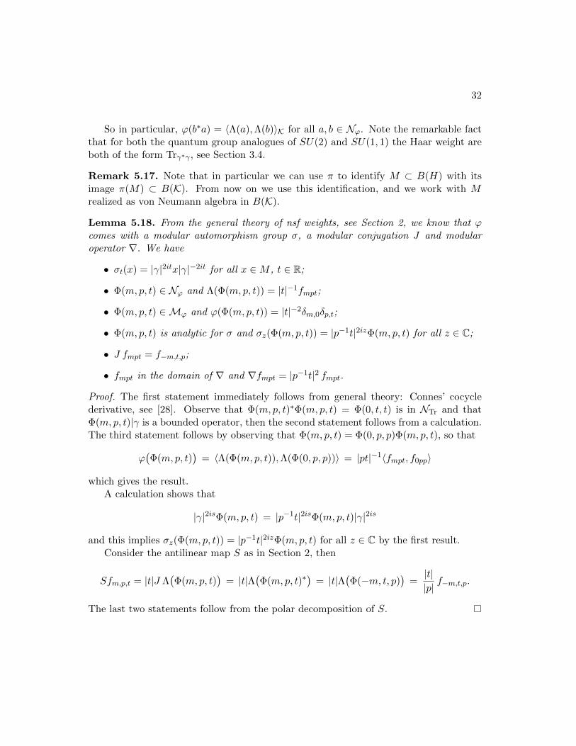
So in particular, ϕ(b∗a) = 〈Λ(a),Λ(b)〉K for all a, b ∈ Nϕ. Note the remarkable factthat for both the quantum group analogues of SU(2) and SU(1, 1) the Haar weight areboth of the form Trγ∗γ , see Section 3.4.

Remark 5.17. Note that in particular we can use π to identify M ⊂ B(H) with itsimage π(M) ⊂ B(K). From now on we use this identification, and we work with Mrealized as von Neumann algebra in B(K).

Lemma 5.18. From the general theory of nsf weights, see Section 2, we know that ϕcomes with a modular automorphism group σ, a modular conjugation J and modularoperator ∇. We have

• σt(x) = |γ|2itx|γ|−2it for all x ∈M , t ∈ R;

• Φ(m, p, t) ∈ Nϕ and Λ(Φ(m, p, t)) = |t|−1fmpt;

• Φ(m, p, t) ∈Mϕ and ϕ(Φ(m, p, t)) = |t|−2δm,0δp,t;

• Φ(m, p, t) is analytic for σ and σz(Φ(m, p, t)) = |p−1t|2izΦ(m, p, t) for all z ∈ C;

• J fmpt = f−m,t,p;

• fmpt in the domain of ∇ and ∇fmpt = |p−1t|2 fmpt.

Proof. The first statement immediately follows from general theory: Connes’ cocyclederivative, see [28]. Observe that Φ(m, p, t)∗Φ(m, p, t) = Φ(0, t, t) is in NTr and thatΦ(m, p, t)|γ is a bounded operator, then the second statement follows from a calculation.The third statement follows by observing that Φ(m, p, t) = Φ(0, p, p)Φ(m, p, t), so that

ϕ(Φ(m, p, t)

)= 〈Λ(Φ(m, p, t)),Λ(Φ(0, p, p))〉 = |pt|−1〈fmpt, f0pp〉

which gives the result.A calculation shows that

|γ|2isΦ(m, p, t) = |p−1t|2isΦ(m, p, t)|γ|2is

and this implies σz(Φ(m, p, t)) = |p−1t|2izΦ(m, p, t) for all z ∈ C by the first result.Consider the antilinear map S as in Section 2, then

Sfm,p,t = |t|J Λ(Φ(m, p, t)

)= |t|Λ

(Φ(m, p, t)∗

)= |t|Λ

(Φ(−m, t, p)

)=|t||p|

f−m,t,p.

The last two statements follow from the polar decomposition of S.

33

5.4 The multiplicative unitary and the comultiplication

The multiplicative unitary W ∈ B(K ⊗ K) has a useful description in terms of thefunctions ap(·, ·), as defined in Definition 5.11,

W ∗(fm1,p1,t1 ⊗ fm2,p2,t2) =∑y,z∈Iq

sgn(p2t2)yzqm2/p1∈Iq

∣∣∣∣ t2y∣∣∣∣ at2(p1, y)ap2(z, sgn(p2t2)yzqm2/p1)

× fm1+m2−χ(p1p2/t2z),z,t1 ⊗ fχ(p1p2/t2z),sgn(p2t2)yzqm2/p1,y.

(5.9)

For convenience we state the corresponding result for W as well, which follows directlyfrom (5.9):

W (fm1,p1,t1 ⊗ fm2,p2,t2) =∑r,s∈Iq

sgn(rp2t2)sp1qm2∈Iq

∣∣∣∣ st2∣∣∣∣ as(sgn(rp2t2)sp1q

m2 , t2) ar(p1, p2)

× fm1−χ(sp2/t2),sgn(rp2t2)sp1qm2 ,t1 ⊗ fm2+χ(sp2/t2),r,s.

(5.10)

Proposition 5.19. W ∈ B(K ⊗K) is unitary operator.

Proof. This follows by a straightforward check using Propositions 5.12 and 5.13.

Now we define the comultiplication ∆(x) = W ∗(1⊗ x)W for x ∈M .

Theorem 5.20. ∆ is coassociative, i.e. (∆⊗ ι) ∆ = (ι⊗∆) ∆.

The proof of Theorem 5.20 is intense and laborious, and we will not repeat it here.The idea is to check it for generators of M , which has certain complications involvingdomains as α and γ are unbounded. We refer to [19] for details.

Theorem 5.21. (M,∆) is a locally compact quantum group with left and right Haarweight ϕ and multiplicative unitary W .

Proof. According to Definition 3.1 and Theorem 5.20 it suffices to check that ϕ is a leftHaar weight and that the right Haar weight can be taken equal to ϕ. This requires somevon Neumann algebra techniques, for which we refer to [19].

34

6 Cocycle twisting

The aim of this section is to present a technique to obtain new quantum groups by ‘twist-ing’ an existing quantum group using a cocycle. It was shown by Fima and Vainerman[14] that for special cases of the cocycle one can indeed obtain an operator algebraicquantum group satisfying all the conditions of the Kustermans-Vaes definition. Thehard part is to show existence of the Haar weights. For general (unitary) cocycles thisresult was obtained by De Commer [8]. In fact De Commer obtains an even more generalresult that led to an alternative approach of defining/finding SUq(1, 1).

6.1 Cocycle twisitng

Let G = (M,∆) be a locally compact quantum group. A cocycle is a unitary Ω ∈ M⊗Mthat satisfies the cocycle relation

(Ω⊗ 1)(∆⊗ ι)(Ω) = (1⊗ Ω)(ι⊗∆)(Ω).

Some texts will speak about unitary cocycles, but we shall simply make that part of thedefinition here. There is an easy way of obtaining a cocycle. Namely, let X ∈ M beunitary. Then

(X ⊗X)∆(X∗) (6.1)

is always a cocycle (it is an easy exercise to verify the cocycle relation). The cocycles ofthe form (6.1) are called coboundaries.

To a cocycle Ω ∈ M⊗M we may associate a new quantum group in the following way.The underlying von Neumann algebra will again be M but then with comultiplication

∆Ω(x) = Ω∆(x)Ω∗.

It follows from the coycle identity that the comultiplication is coassociative. Indeed,

(∆Ω ⊗ ι) ∆Ω(x)

=(Ω⊗ 1)(∆⊗ ι)(Ω∆(x)Ω∗)(Ω∗ ⊗ 1)

=(Ω⊗ 1)(∆⊗ ι)(Ω) × (∆⊗ 1)∆(x) × (∆⊗ ι)(Ω∗)(Ω∗ ⊗ 1)

=(1⊗ Ω)(ι⊗∆)(Ω∆(x)Ω∗)(1⊗ Ω∗)

=(ι⊗∆Ω) ∆Ω(x).

Note that if Ω is a coboundary, say Ω = (X ⊗X)∆(X∗) with X ∈ M unitary, then thetwisted pair (M,∆Ω) is isomorphic to (M, ϕ). Indeed the map x 7→ XxX∗ gives thisisomorphism. What is not so trivial is that in general (M,∆Ω) admits Haar weightswhich turn it into a locally compact quantum group.

Theorem 6.1 (See [8]). There exist Haar weights ϕΩ, ψΩ such that the 4-tuple GΩ =(M,∆Ω, ϕΩ, ψΩ) is a locally compact quantum group.

35

We will give the main ingredients of the proof of this theorem in this section, whichare more general Galois co-objects. Every result here is proved by De Commer in [8],see also his thesis [7] which contains a couple of additional results (partly unpublished).Before going into details let us also mention the following.

Theorem 6.2 (See [9]). Let G be a compact quantum group. The twisted quantum groupGΩ is not necessarily compact.

Let us give the idea behind Theorem 6.2, at least to some extend. Firstly let us recallsomething on infinite tensor products of Von Neumann algebras, see [29, Section XIV.1].Let (Mk, ϕk) be von Neumann algebras equipped with normal, faithful state ϕk indexedby k ∈ N. Then we may construct an infinite tensor product ⊗k(Mk, ϕk) as follows.Let (Hk, ξk) be its GNS space with cyclic vector ξk. We have a canonical embedding⊗nk=0Hk → ⊗

n+1k=0Hk by means of the mapping (⊗nk=0ηk) 7→ (⊗nk=0ηk)⊗ ξn+1. This turns

⊗nk=0Hk → ⊗n+1k=0Hk,

into an inductive system of Hilbert spaces of which we may take the direct limit which wedenote by ⊗∞k=0Hk. The embedding of a finite tensor η0⊗ . . .⊗ ηn ∈ ⊗nk=0Hk in ⊗∞k=0Hkis given by η0 ⊗ . . .⊗ ηn ⊗ ξn+1 ⊗ ξn+2 ⊗ . . .. This way the finite tensors ⊗nk=0Mk act on⊗∞k=0Hk and the double commutant of ∪n ⊗nk=0 Mk is by definition ⊗∞k=0(Mk, ϕk). Weemphasize that the construction does depend on the choice of the states. For example,take (Mk, ϕk) = (M2(C),Tr( ·A)) with A the matrix given by

A =

(α 00 1− α

), 0 < α ≤ 1

2.

Then ⊗∞k=0(Mk, ϕk) is the hyperfinite IIIλ-factor with λ = α1−α in case 0 < α < 1

2 . And

⊗∞k=0(Mk, ϕk) is the hyperfinite II1-factor in case α = 12 , see [29] (it is also summarized

in [6]).The idea behind Theorem 6.2 is – very roughly – to take for the quantum group G

an infinite tensor product of SUqk(2) for parameters qk that satisfy∑

k q2k < ∞. The

tensor product is taken with respect to the Haar states. Recall that the von Neumannalgebra of SUqk(2) is given by B(`2(N))⊗ L∞(T). Define the unitary,

wk =

0 1 0 00 0 1 01 0 0 00 0 0 I

⊗ 1 ∈ B(`2(N))⊗ L∞(T).

In [9] it is shown that Ω := ⊗∞k=0(wk ⊗ wk)∆(w∗k) is a well-defined element of the vonNeumann algebra of (⊗∞k=0SUqk(2))⊗ (⊗∞k=0SUqk(2)) that satisfies the cocycle relation.Then twisting ⊗∞k=0SUqk(2) with Ω turns out to yield a non-compact quantum group.Note that whereas the tensor legs (wk ⊗ wk)∆(w∗k) are coboundaries, the cocycle Ω isnot a coboundary (as then the twist would be compact again).

36

6.2 Twisting by Galois coobjects

In this section we review the construction from [8]. The input is a Galois coobject theoutput is a new quantum group, of which cocycle twists are a special case. Therefor fixa locally compact quantum group (M, ϕ).

Definition 6.3. A coaction of (M, ϕ) on a von Neumann algebra N is a normal ∗-homomorphism α : N→ M⊗N satisfying the relation (∆⊗ ι)α = (ι⊗α)α. We definethe fixed point algebra as

Nα := x ∈ N | α(x) = 1⊗ x .

The coaction is called ergodic if Nα = C1. A coaction is called integrable if (ϕ⊗ ι) α :N+ → N+ is a semi-finite operator valued weight.

Remark 6.4. What we defined as coaction is sometimes called a left coaction, where aright coaction would mean that α maps N→ N⊗M and the rest of the definition changesaccordingly.

From this point we shall fix a coaction α : N → M ⊗ N that is both integrable andergodic. Note that we have (ϕ ⊗ ι) α : N → Nα ' C so that (ϕ ⊗ ι) α is a normalsemi-finite faithful weight (and not just an operator valued weight). We assume that Nis equipped with this weight from now on. A particular case of this situation is whereα = ∆, the comultiplication of M. The constructions below then ‘trivialize’ meaningthat the twisted quantum group we shall obtain equals (M, ϕ) it self. Let us now carryout the constructions of [8]. Firstly we recall the definition of the crossed product, see[34].

Definition 6.5. The crossed product von Neumann algebra N oα M is defined as thevon Neumann algebra algebra acting on L2(N)⊗L2(M) that is generated by 1⊗ M′ andα(N).

To the action α we may associate the following operator that resembles the multi-plicative unitary:

G : L2(N)⊗L2(N)→ L2(N)⊗L2(M) : (ΛN⊗ΛN)(x⊗y) 7→ (ΛN⊗ΛM)(α(x)(y⊗1)). (6.2)

We also set G = ΣG : L2(N) ⊗ L2(N) → L2(M) ⊗ L2(N), where Σ : L2(N) ⊗ L2(M) →L2(M)⊗ L2(N) is the flip map. It is not hard to check that G is an isometry (the proofis the same as for the definition of W ∗) and hence in particular (6.2) is a well-definedand bounded map. If α = ∆ then in fact G = W ∗. In general G is not a unitary mapand therefore we introduce the following definition at this point.

Definition 6.6. We call an integrable, ergodic coaction α a Galois coaction if the map(6.2) is unitary.

37

Remark 6.7. There is an alternative – perhaps better – way of defining a Galois coac-tion. Assume that (M,∆) = (L∞(G),∆G) is a classical group and G acts on a measurespace (X,µ), call this action (g, x) 7→ βg(x). Given g ∈ G we let β∗g ∈ B(L2(X)) be thepull back of this map. Let α : L∞(X,µ)→ L∞(G)⊗ L∞(X) ' L∞(G×X) : f 7→ f β.We shall assume that α is ergodic and integrable. Then we may define the Galois ho-momorphism, see [34, Theorem 5.3], which is the normal ∗-homorphism given by,

ρ : L∞(X,µ) oα G→ B(L2(X,µ)),

which is determined by

α(x) 7→ x,∫Gf(s)ρsds 7→

∫Gf(s)

(dµ βsdµ

) 12

β∗sds.

Because α is ergodic the map ρ is in fact surjective. It turns out that ρ is an isomor-phism if and only if the operator G introduced above is unitary, see [8, Theorem 2.1].These constructions can be generalized to arbitrary locally compact quantum groupsand [8, Theorem 2.1] holds in fact in full generality. We did not introduce these generalconstructions here as this would mean that we had to introduce several new objects first(such as the unitary implementation of a coaction from [34]).

We now set

O :=

(ι⊗ ω)(G) | ω ∈ B(L2(N))σ-wk

⊆ B(L2(N), L2(M)),

and N := O∗ ⊆ B(L2(M), L2(N)). Finally put P to be the closed linear span of ON.Define

∆N

: N→ N⊗ N :x 7→ G∗(1⊗ x)W,

∆O

: O→ O⊗ O :x 7→ (∆N

(x∗))∗,

∆P

: P→ P⊗ P :x 7→ G∗(1⊗ x)G.

One of the main results of [8] is that (P ,∆P

) admits left and right Haar weights thatcomplete it to a locally compact quantum group. Moreover(

P O

N M

)together with the pointwise application of(

∆P

∆O

∆N

∆M

):

(P O

N M

)→

(P ⊗ P O ⊗ ON ⊗ N M ⊗ M

)determines a locally compact quantum groupoid with base space M2(C).

38

Remark 6.8. This is just a very brief account of what happens in [8]. Note that in [8]the spaces N , O, P are introduced in a different way. They are the intertwining algebrasbetween suitable representations of the von Neumann algebra N on L2(N) and L2(M).The representation of N on L2(M) requires again the (fully general) Galois isomorphismfrom Remark 6.7. As we have chosen not to include this Galois map in these notes wehave given the alternative definition above.

Theorem 6.9. Let Ω ∈ M⊗M be a cocycle. Then there is a Galois coobject N of (M,∆)

such that the twisted quantum group P(=P) constructed above equals the cocycle twist

(M,∆Ω).

Proof. We give a proof sketch, i.e. we say how to construct the Galois coobject. It relieson crossed product duality. We let

N := CoΩ M = (ω ⊗ ι)(WΩ∗) | ω ∈ M∗,

be the twisted crossed product of the trivial action of (M, ∆). By crossed product duality[32] there exists a dual coaction α : N→ N⊗M of (M,∆) on N that is determined by

α((ω ⊗ ι)(WΩ∗)) = (ω ⊗ ι⊗ ι)(W13W12Ω∗12),

with ω ∈ M∗. This turns N into a Galois coaction for (M,∆). We refer to [8] fordetails.

6.3 Concluding remarks about SUq(1, 1)

In [10] it is shown that there exists a Galois coobject for SUq(2) such that the twistedquantum group equals SUq(1, 1). The coobject turns out to be a Podles sphere. Notethat we really mean the dual of SUq(2) and not SUq(2) itself. Such Galois coobjects canbe found through projective corepresentations of SUq(2), see [8]. Using crossed productduality it is in fact shown that these projective corepresentations of a quantum groupare in 1–1 correspondence with Galois coobjects of the dual quantum group.

The advantage of this approach is that the coassociativity of the comultiplicationof the twisted group is automatic: the problem reduces/changes from constructing aquantum group to identifying a quantum group. That is, one really has to show thatthe outcoming quantum group is a suitable form of SUq(1, 1). This is in general not sotrivial (though in some examples it is known by now) as from the twisting procedureit is not so clear which quantum group one a priori obtains. The hope/aim/guess is ofcourse that these methods can be used to find higher rank versions of these quantumgroups.

Finally we need to comment that the presentation in this chapter is highly simplified.The full theory can be found in [7] which includes the universal and reduced C∗-algebraictheory as well as a more “global” picture of monoidal/morita equivalences.

39

References

[1] O. Bratteli, D. Robinson, Operator algebras and quantum statistical mechanics. Vol1., Texts and Monographs in Physics. Springer-Verlag, New York-Heidelberg, 1979.xii+500 pp.

[2] M. Caspers, The Lp-Fourier transform on locally compact quantum groups, J. Oper-ator Theory 69 (2013), 161–193.

[3] M. Caspers, Weak amenability of locally compact quantum groups and approximationproperties of extended quantum SU(1, 1), Comm. Math. Phys. 331 (2014), no. 3,1041–1069.

[4] M. Caspers, E. Koelink, Lecture notes quantum groups and special functions, Win-ter school Bizerte 2010, available at: http://www.math.ru.nl/ koelink/edu/GQSF-Bizerte-2010.pdf.

[5] M. Caspers, E. Koelink, Modular properties of matrix coefficients of corepresentationsof a locally compact quantum group, J. Lie Theory 21 (2011), no. 4, 905–928.

[6] M. Caspers, D. Potapov, F. Sukochev, The Walsh basis in the Lp-spaces of hyperfiniteIIIλ factors, 0 < λ ≤ 1, J. Math. Anal. Appl. 408 (2013), 154–164.

[7] K. de Commer, Phd Thesis, available at http://homepages.vub.ac.be/

~kdecomme/.

[8] K. de Commer, Galois objects and cocycle twisting for locally compact quantumgroups, J. Operator Theory 66 (2011), 59–106.

[9] K. De Commer, On cocycle twisting of compact quantum groups, J. Funct. Anal. 258(2010), no. 10, 3362–3375

[10] K. De Commer, On a correspondence between quantum SU(2), quantum E(2) and˜SU(1, 1), Comm. Math. Phys. 304 (2011), no. 1, 187–228.

[11] K. de Commer, On a Morita equivalence between the duals of quantum SU(2) andquantum E(2), Adv. Math. 229 (2012), 1047–1079.

[12] K. de Commer, S. Neshveyev, Quantum flag manifolds as quotients of degeneratequantized universal enveloping algebras, arXiv: 1402.4249.

[13] J. Dixmier, “Les algebres d’operateurs dans l’espace hilbertien”, Gauthiers-Villars,1957.

[14] P. Fima, L. Vainerman, Twisting and Rieffel’s deformation of locally compact quan-tum groups. Deformation of the Haar measure, Commun. Math. Phys. 286 2009, no.3, 1011–1050.

40

[15] G. Gasper, M. Rahman, Basic Hypergeometric Series, Cambridge Univ. Press 1990.

[16] W. Groenevelt, E. Koelink, J. Kustermans, The dual quantum group for the quantumgroup analogue of the normalizer of SU(1, 1) in SL(2,C), IMRN 7 (2010), 1167–1314.

[17] A. Jacobs, The quantum E(2) group, PhD thesis, KU Leuven 2005.

[18] P. Kasprzak, On a certain approach to quantum homogeneous spaces, Comm. Math.Phys. 313 (2012), no. 1, 237–255.

[19] E. Koelink, J. Kustermans, A locally compact quantum group analogue of the nor-malizer of SU(1, 1) in SL(2,C), Comm. Math. Phys. 233 (2003), 231–296.

[20] L.I. Korogodsky, Quantum Group SU(1, 1)oZ2 and super tensor products, Comm.Math. Phys. 163 (1994), 433–460.

[21] J. Kustermans, A. Van Daele, C∗-algebraic quantum groups arising from algebraicquantum groups, Int. J. Math. Vol. 8, No. 8 (1997), 1067–1139.

[22] J. Kustermans, S. Vaes, Locally compact quantum groups, Ann. Scient. Ec. Norm.Sup. 33 (2000), 837–934.

[23] J. Kustermans, S. Vaes, Locally compact quantum groups in the von Neumann al-gebraic setting, Math. Scand. 92 (2003), 68–92.

[24] J. Kustermans, Locally compact quantum groups in the universal setting, Internat.J. Math. 12 (2001).

[25] R. Meyer, S. Roy, S.L. Woronowicz, Homomorphisms of quantum groups, MunsterJ. Math., 5 (2012), 1–24.

[26] S. Stratila, L. Zsido, Lectures on von Neumann algebras, Revision of the 1975 origi-nal. Translated from the Romanian by Silviu Teleman. Editura Academiei, Bucharest;Abacus Press, Tunbridge Wells, 1979.

[27] M. Takesaki, Theory of operator algebras I, Springer 1979.

[28] M. Takesaki, Theory of operator algebras II, Springer 2000.

[29] M. Takesaki, Theory of operator algebras III, Springer 2003.

[30] T. Timmermann, An invitation to quantum groups and duality, EMS 2008.

[31] S. Vaes, A Radon-Nikodym theorem for von Neumann algebras, J. Operator Theory46 (2001), no. 3, 477–489.

[32] S. Vaes, L. Vainerman, Extensions of locally compact quantum groups and the bi-crossed product construction, Advances in Mathematics 175 (2003), no. 1, 1–101.

41

[33] S. Vaes, PhD thesis, available at https://perswww.kuleuven.be/ u0018768/PhD.html.

[34] S. Vaes, The unitary implementation of a locally compact quantum group action, J.Funct. Anal. 180 (2001), 426–480.

[35] A. Van Daele, Locally compact quantum groups. A von Neumann algebra approach,arXiv:math/0602212 (2006).

[36] S. L. Woronowicz, Compact matrix pseudogroups, Comm. Math. Phys. 111 (1987),613–665

[37] S.L. Woronowicz, Unbounded elements affiliated with C∗–algebras and non-compactquantum groups, Comm. Math. Phys. 136 (1991), 399–432.