Lecture Notes on Info-Gap Uncertainty - Technion

Lecture Notes on Info-Gap UncertaintyYakov Ben-Haim

Faculty of Mechanical EngineeringTechnion — Israel Institute of Technology

Haifa 32000 [email protected]

Source material: Yakov Ben-Haim, 2006, Info-Gap Decision Theory: Decisions Under SevereUncertainty, 2nd edition, Academic Press. Chapter 2.A Note to the Student: These lecture notes are not a substitute for the thorough study ofbooks. These notes are no more than an aid in following the lectures.

Contents

1 Central Ideas 2

2 Risk and Uncertainty 32.1 Three-Box Riddle: Probabilistic Version . . . . . . . . . . . . . . . . . . . . . 32.2 Three-Box Riddle: Non-Probabilistic Version . . . . . . . . . . . . . . . . . . . 7

3 Principle of Indifference 83.1 2-Envelope Riddle . . . . . . . . . . . . . . . . . . . . . . . . . . . . . . . . . . 93.2 Keynes’ Example . . . . . . . . . . . . . . . . . . . . . . . . . . . . . . . . . . 103.3 Shackle-Popper Indeterminism . . . . . . . . . . . . . . . . . . . . . . . . . . . 123.4 Influenza Pandemic . . . . . . . . . . . . . . . . . . . . . . . . . . . . . . . . . 13

4 Historical Perspectives onReasoning and Uncertainty 15

5 Info-gap Uncertainty, Probability and Fuzziness 17

6 Some Info-gap Models of Uncertainty 216.1 Energy-bound Models . . . . . . . . . . . . . . . . . . . . . . . . . . . . . . . 226.2 Envelope-bound Models . . . . . . . . . . . . . . . . . . . . . . . . . . . . . . 236.3 Slope-bound info-gap models . . . . . . . . . . . . . . . . . . . . . . . . . . . . 256.4 Fourier-bound info-gap models . . . . . . . . . . . . . . . . . . . . . . . . . . . 25

7 Why Convex Info-gap Models? 267.1 Most Info-Gap Models are Convex: Examples . . . . . . . . . . . . . . . . . . 267.2 Why Are Most Info-Gap Models Convex? . . . . . . . . . . . . . . . . . . . . . 28

0\lectures\risk\lectures\igunc.tex 10.12.2019 c© Yakov Ben-Haim 2019.

1

\lectures\risk\lectures\igunc.tex Notes on Info-gap Uncertainty 2

1 Central Ideas

¶ Decisions.• Decisions:◦ Have consequences: survival, reward, punishment, etc.◦ Are made under uncertainty, competition, resource deficiency.

• Animals:◦ Evolve subject to real world constraints.◦ Make decisions.

• Homo sapiens:◦ Thinker.◦ Tool maker. Tools implement decisions, and gather information to support decision

making.◦ Decision maker.— Psychology: relation to evolution.

Some decision strategies “feel good”.Some decision strategies enhance survival.Evolution links these two categories.

— Knowledge: relation to real world constraints.• Decision strategies: what strategies are available?

¶ Decision strategies:• Satisficing: Doing good enough. Beating the competition.• Optimizing:◦ Use best model to find most rewarding decision.◦ Psychology: Optimizers have more than satisficers, but satisficers are happier (Schwarz).

• Windfalling: Exploiting opportunity; facilitating better-than-expected outcomes.• Which strategy to use? When?

¶ Robust-Satisficing:• Satisficing is sub-optimal, therefore multiple solutions.• Use extra DoF’s to robustify against surprise.• Robustness and probability of success:◦ Animal foraging seems to be robust-satisficing, not intake-maximization.◦ Why? Survival value: greater probability of attaining critical need.

¶ Robustness and Opportuneness: Antagonism or sympathy?

¶ The big challenge: uncertainty.• What is uncertainty?◦ Epistemic.◦ Ontological.

• How to model and manage uncertainty?◦ Probability and statistics.◦ Info-gap theory.◦ Fuzzy logic.◦ Dempster-Shafer theory.◦ More.

• We will focus on probability and info-gap theory.


2 Risk and Uncertainty

2.1 Three-Box Riddle: Probabilistic Version

¶ Background to the riddle:• Prize in 1 of 3 boxes.• We must choose a box:

? ? ?

• We know prior probabilities are equal: P1 = P2 = P3 = 1/3.Pi = probability that prize is in ith box.

• For choice of box i, the probability of failure is:

Pf = 1− Pi =2

3(1)

• We choose a box, call it ‘C’.

C ? ?

• Then the M.C., who knows where the prize is, opens a box, ‘E’, and shows us that itis empty:

C E T

The third box, ‘T’, remains closed.

¶ The Riddle: is there a rational basis for changing our choice? C =⇒ T?

¶ Probabilistic analysis:• Our prior knowledge is: Prob(C) = 1/3.• By normalization of the probability: Prob(not C) = 1− Prob(C) = 2/3.• The prize being in ‘E’ or in ‘T’ are disjoint events. Thus:

Prob(not C) = Prob(E or T ) = Prob(E) + Prob(T )• After the M.C. opens ‘E’, we know that Prob(E) = 0.• Thus Prob(T ) = 2/3.• Thus changing from ‘C’ to ‘T’ increases the probability of success by a factor of two!

Hence: change the choice.


¶ Skeptical? Consider the 1000-box version:• Prize in 1 of 1000 boxes.• We know prior probabilities are equal: P1 = · · · = P1000 = 1/1000.• For choice of box i, the probability of failure is:

Pf = 1− Pi = 0.999 (2)

• We choose a box, call it ‘C’.• Then the M.C., who knows where the prize is, opens and shows us 998 empty boxes,

leaving ‘C’ and ‘T’ closed.• Question: is there a rational basis for changing our choice? C =⇒ T?

¶ Probabilistic analysis:• Our prior knowledge is: Prob(C) = 0.001.• By normalization of the probability: Prob(not C) = 1− Prob(C) = 0.999.• Let ‘E’ denote the 998 empty boxes.• The prize being in ‘E’ or in ‘T’ are disjoint events. Thus:

Prob(not C) = Prob(E or T ) = Prob(E) + Prob(T )• After the M.C. opens 998 empty boxes, we know that their cumulative probability is

zero: Prob(E) = 0.• Thus Prob(T ) = 0.999.• Thus changing from ‘C’ to ‘T’ increases the probability of success by a factor of 999.

Hence: change the choice.


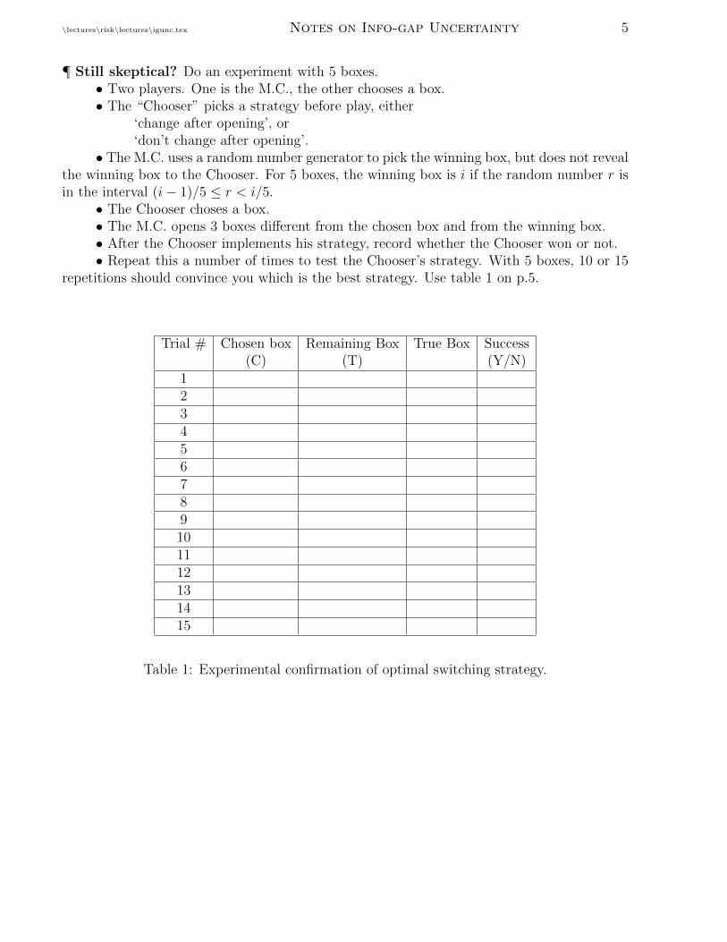
¶ Still skeptical? Do an experiment with 5 boxes.• Two players. One is the M.C., the other chooses a box.• The “Chooser” picks a strategy before play, either

‘change after opening’, or‘don’t change after opening’.

• The M.C. uses a random number generator to pick the winning box, but does not revealthe winning box to the Chooser. For 5 boxes, the winning box is i if the random number r isin the interval (i− 1)/5 ≤ r < i/5.

• The Chooser choses a box.• The M.C. opens 3 boxes different from the chosen box and from the winning box.• After the Chooser implements his strategy, record whether the Chooser won or not.• Repeat this a number of times to test the Chooser’s strategy. With 5 boxes, 10 or 15

repetitions should convince you which is the best strategy. Use table 1 on p.5.

Trial # Chosen box Remaining Box True Box Success(C) (T) (Y/N)

123456789101112131415

Table 1: Experimental confirmation of optimal switching strategy.


¶ Return to the 3-box problem, in more general form:• Prize in 1 of 3 boxes, and we must choose a box.• We know prior probabilities, P1, P2, P3, but they are not necessarily equal.• For choice of box i, the probability of failure is:

Pf = 1− Pi (3)

• We choose a box, call it ‘C’.• Then the M.C., who knows where the prize is, opens an empty box, ‘E’.• Question: is there a rational basis for changing our choice? C =⇒ T?

¶ General Probabilistic analysis:• Known prior probability distribution: P1, P2, P3.• Our prior knowledge is: Prob(C) = PC which is known.• By normalization of the probability: Prob(not C) = 1− PC .• The prize being in ‘E’ or in ‘T’ are disjoint events. Thus:

Prob(not C) = Prob(E or T ) = Prob(E) + Prob(T )• After the M.C. opens ‘E’, we know that Prob(E) = 0.• Thus Prob(T ) = 1− PC .• Change from ‘C’ to ‘T’ if and only if 1− PC > PC :

Change if: PC < 1/2 (4)

Don’t change if: PC > 1/2 (5)

Indifferent if: PC = 1/2 (6)

• Conclusions:◦ There is an infinity of prior distributions P1, P2, P3 for which we would not

change the chosen box.◦ There is an infinity of prior distributions P1, P2, P3 for which we would change

the chosen box.◦ The choice of a strategy depends upon knowledge of the prior probability distri-

bution.


2.2 Three-Box Riddle: Non-Probabilistic Version

¶ Background to the problem:• Prize in 1 of 3 boxes.• We must choose a box: ? ? ?• We do not know the prior probabilities, P1, P2, P3.• If Pi > 1/2 then we would choose box i and stick with it.

¶ Can we guess the prior probabilities?• Suppose we have a rough guess of the prior distribution. How should we use this

information?• Can we use the principle of indifference to choose the prior distribution?• Principle of indifference: ascribe equal probabilities to elementary events about

which no other information is available. Hence uniform distribution:

(P1, P2, P3) = (1/3, 1/3, 1/3) (7)

◦ Uniform distribution has maximum entropy:

H(P1, P2, P3) = −3∑

N=1

PN lnPN

From among all possible probability distributions.◦ ‘Max entropy’ does not imply ‘no information’.

◦ Knowing a specific probability distribution is knowledge.

¶ The uncertainty is an information gapbetween what we do know and what we need to know.

• We have no information, not even probabilistic.


3 PRINCIPLE of INDIFFERENCE

§ Question:Is ignorance probabilistic?

§ Principle of indifference (Bayes, LaPlace, Jaynes, . . . ):• Elementary events, about which nothing is known, are assigned equal probabilities.• Uniform distribution represents complete ignorance.

§ The info-gap contention:The probabilistic domain of discourse does not encompass all epistemic uncertainty.

§ We now consider some paradoxical implications of the principle of indifference.


3.1 2-Envelope Riddle

§ The riddle:• You are presented with two envelopes.◦ Each contains a positive sum of money.◦ One contains twice the contents of the other.

• You choose an envelope, open it, and find $50.

• Would you like to switch envelopes?

§ You reason as follows:

• Other envelope contains either $25 or $100.• Principle of indifference:• Assume equal probabilities.

The expected utility upon switching is:

E.U. = 12

$25 + 12

$100= $62.50.

$62.50 > $50.• Yes! Let’s switch, you say.

§ The riddle, re-visited:• You are presented with two envelopes.◦ Each contains a positive sum of money.◦ One contains twice the contents of the other.• You choose an envelope, but do not open it.• Would you like to switch envelopes?

§ You reason as follows:

• This envelope contains $X > $0.

• Other envelope contains either $2X or $ 12X .

• Principle of indifference:• Assume equal probabilities.

The expected utility upon switching is:

E.U. = 12

$2X + 12

$ 12X = $

(1+ 1

4

)X > X .

• Yes! Let’s switch, you say.§ You wanna switch again? And again? And again?


3.2 Keynes’ Example

§ ρ = specific gravity [g/cm3] is unknown:

1 ≤ ρ ≤ 3

§ Principle of indifference:

Uniform distribution in [1, 3], so:

-

6

1 3ρ

P (ρ)

§ Uniform distribution in [1, 3], so:

PROB

(32≤ ρ ≤ 3

)=34

-

6

14

34

1 32

3ρ

P (ρ)


§ φ = specific volume [cm3/g] is unknown:

13≤ φ ≤ 1


Uniform distribution in[13, 1

], so:

-

6

13

1φ

P (φ)


Uniform distribution in[13, 1

], so:

PROB

(13≤ φ ≤ 2

3

)=12

-

6

12

12

13

23

1φ

P (φ)

§ Note that the following events are identical:

1

3≤ φ ≤ 2

3≡ 3

2≤ ρ ≤ 3 (8)


§ Contradiction:

12

= PROB

(13≤ φ ≤ 2

3

)︸︷︷︸

Specific volume

= PROB

(32≤ ρ ≤ 3

)︸︷︷︸

Specific gravity

=34

§ The Culprit:• Principle of indifference.

§ The resolution:• Ignorance is not probabilistic.• Ignorance is an info-gap.

3.3 Shackle-Popper Indeterminism

§ Intelligence:What people know,influences how they behave.

§ Discovery:What will be discovered tomorrowcannot be known today.

§ Indeterminism:Tomorrow’s behavior cannot bemodelled completely today.

§ Information-gaps, indeterminisms,sometimescannot be modelled probabilistically.

§ Ignorance is not probabilistic.


3.4 INFLUENZA PANDEMIC

This section is based on the following World Health Organization (WHO) website:http://www.who.int/csr/disease/avian influenza/enThe following is a quote from that site:

Estimating the impact of the next influenza pandemic: enhancing preparednessGeneva, 8 December 2004Influenza pandemics are recurring and unpredictable calamities. WHO and influenza expertsworldwide are concerned that the recent appearance and widespread distribution of an avianinfluenza virus, Influenza A/H5N1, has the potential to ignite the next pandemic.Give the current threat, WHO has urged all countries to develop or update their influenzapandemic preparedness plans (see information on web pages below) for responding to thewidespread socioeconomic disruptions that would result from having large numbers of peopleunwell or dying.— Pandemic preparednessCentral to preparedness planning is an estimate of how deadly the next pandemic is likelyto be. Experts’ answers to this fundamental question have ranged from 2 million to over50 million. All these answers are scientifically grounded. The reasons for the wide range ofestimates are manyfold.Some estimates are based on extrapolations from past pandemics but significant details ofthese events are disputed, including the true numbers of deaths that resulted. The mostprecise predictions are based on the pandemic in 1968 but even in this case estimates varyfrom one million to four million deaths. Similarly, the number of deaths from the Spanishflu pandemic of 1918 is posited by different investigators to range from 20 million to wellover 50 million. Extrapolations are problematic because the world in 2004 is a different placefrom 1918. The impact of greatly improved nutrition and health care needs to be weighedagainst the contribution the increase in international travel would have in terms of globalspread. The specific characteristics of a future pandemic virus cannot be predicted. It mayaffect between 20-50% of the total population. It is also unknown how pathogenic a novelvirus would be, and which age groups will be affected. The level of preparedness will alsoinfluence the final death toll. Even moderate pandemics can inflict a considerable burdenon the unprepared and disadvantaged. Planning to maintain health care systems will beespecially crucial. Good health care will play a central role in reducing the impact, yet thepandemic itself may disrupt the supply of essential medicines and health care workers mayfall ill. Because of these factors, confidently narrowing the range of estimates cannot be doneuntil the pandemic emerges. Therefore, response plans need to be both strong and flexible.Even in the best case scenarios of the next pandemic, 2 to 7 million people would die andtens of millions would require medical attention. If the next pandemic virus is a very virulentstrain, deaths could be dramatically higher.The global spread of a pandemic cannot be stopped but preparedness will reduce its impact.WHO will continue to urge preparedness and assist Member States in these activities. In thenext few weeks, WHO will be publishing a national assessment tool to evaluate and focusnational preparedness efforts. WHO will also be providing guidance on stockpiling antiviralsand vaccines. Next week, WHO will be convening an expert meeting on preparedness planning.WHO is also working to advance development of pandemic virus vaccines, and to expediteresearch efforts to understand the mechanisms of emergence and spread of influenza pandemics.It is of central importance that Member States take the necessary steps to develop their ownpreparedness plans. Some have already developed structures and processes to counter this


threat but some plans are far from complete and many Member States have yet to begin.WHO believes the appearance of H5N1, which is now widely entrenched in Asia, signals thatthe world has moved closer to the next pandemic. While it is impossible to accurately forecastthe magnitude of the next pandemic, we do know that much of the world is unprepared for apandemic of any size.


4 Historical Perspectives on Reasoning and Uncertainty

(Ch. 2, sec. 1, pp.9–12)¶ Four stages:

I. Deduction: ancient Greece . . .II. Forward probability: 1600, Pascal, Fermat, . . .III. Inverse probability: 1760, Bayes, . . .IV. Modern inference.

I. Symbolic Logic, mathematical deduction:• Axiomatic geometry (Euclid, c.200 BCE)• Symbolic logic, syllogism (Aristotle, c.200 BCE):

1. All men are mortal.2. Socrates is a man.3. Therefore Socrates is mortal.

II. Games of chance (Pascal, Fermat, etc., 1600 . . . )• Forward probability:

Given known coin, what is the probability of any specified sequence?• Probabilistic syllogism for sequence of coin flips with known coin: pH , pT known.

1. Probability of specific sequence of Heads and Tails is calculated as pNHH pNT

T .2. Given the specific sequence HHTH.3. Hence the probability of HHTH is known and equals . . . .

III. Inference: Inverse probability.• Given unknown coin, which has produced a given sequence,

what are the probabilities of the individual basic events?(Bayes, 1760, studying dice).

• Least-squares estimation:Given noisy measurements of celestial motions,what is the best estimate of an elliptical orbit?(Gauss, Legendre, 1800)

• Central limit theorem (Laplace 1815):Given measured mean and variance, we know the pdf.

• Many other distributions and associated statistical tests.(Karl Pearson and many others, 19th, 20th c.)

• Probabilistic syllogism for sequence of coin flips:1. If probabilities of Heads and Tails are PH , PT ,

Then probability of observation is P (HHTH|PH , PT ).2. Observed sequence HHTH.3. Hence estimates of PH , PT are . . .


IV. Modern design, decision and inference.• Verbal uncertainty (Lukaceiwizc, 1920; Zadeh, 1960).

“If it rattles, tighten it.”Uncertainties:

What is a rattle?How tight is tight?• Innovation under time-pressure.• New manufacturing technologies:

Exchangeable parts, assembly line, automation, robotics, etc.• New managerial techniques:

planning, distributed control, data bases, networks, etc.• New materials:

plastics, superconductors, etc.• New scientific discoveries:

solid state physics, quantum effects, etc.• Uncertainties:◦ Lack of data, information, understanding.◦ Mutually inconsistent data.◦ Disparity between

what is knownand what must be knownfor a good decision.

This is information-gap uncertainty.

¶ Each stage evolved

new modes of reasoningin order to deal with

new problems

¶ Summary of stages:I. Deduction:

Mathematical question with unique inescapable answer.II. Forward probability:

Math applied to uncertainty, with unique inescapable answer.III. Inverse probability:

Math applied to uncertainty, with non-unique or incomplete answer.IV. Modern high-speed decision-making:

Severe uncertainty; info-gaps.


5 Info-gap Uncertainty, Probability and Fuzziness

¶ Three models/conceptions of uncertainty:• Probability:◦ Frequency of recurrence.P (X) = frequency with which X recurs.◦ Degree of belief.P (X) = degree to which I believe X will occur.◦ In both cases:P (X) + P (¬X) = 1. (‘¬X’ means ‘not X’)

• Fuzzy logic:◦ Linguistic ambiguity.◦ Possibility (less strict than probability).M(X) = possibility that X (e.g., rain tomorrow) will occur.M(X) +M(¬X) > 1. Both ‘rain’ and ‘not rain’ are highly possible.◦ Necessity (more strict than probability).M(X) = neccesity that X (e.g., rain tomorrow) will occur.M(X) +M(¬X) < 1. There may be heavy dew,

which is neither ‘rain’ nor ‘not rain’.• Info-gap:◦ Clustering of events.◦ Disparity between the known and the learnable.

We will compare these three briefly.

¶ Fuzzy logic is a major break away from probability.However, both F.L. and probability use:

normalized measure functions(pdf or membership functions)

to assess uncertainty.

¶ Info-gap models have no measure functions.


¶ Example: Toxic waste.• Toxic waste is released from industrial plant into river.• The waste causes damage to plants, animals, humans.• The waste is removed by various processes:◦ Chemical reaction, adsorption, absorption.• These are very complex processes. Depend on many factors:◦ Time, temperature, concentration, surface conditions, etc.• Accurate model of removal rate: very expensive.• r(x, t, w) = current best model of removal rate.◦ x = position, t = time, w = other parameters.• r(x, t, w) may be simple or complex.• r(x, t, w) = unknown true model of removal rate.• r(x, t, w) and r(x, t, w) differ in unknown ways.• Too little info and understanding to evaluate:◦ probability of deviation of r from r.◦ plausibility of deviation of r from r.• Neither probabilistic nor fuzzy uncertainty model is accessible.• Severe uncertainty. Use info-gap model for uncertainty in r(x, t, w).• Family of nested sets of r-functions.


¶ Fractional-error info-gap model for uncertainty in r(x, t, w):

U(h, r) =

{r(x, t, w) :

∣∣∣∣∣ r(x, t, w)− r(x, t, w)

r(x, t, w)

∣∣∣∣∣ ≤ h

}, h ≥ 0 (9)

h is the unknown horizon of uncertainty.r(x, t, w) is the nominal model.

¶ Two levels of uncertainty:• Unknown fractional error of r in U(h, r) at given h.• Unknown horizon of uncertainty, h.

¶ Nesting of info-gap models:

h < h′ =⇒ U(h, r) ⊆ U(h′, r) (10)

¶ Contraction of info-gap models:U(0, r) = {r} (11)

¶ Info-gap models organize events into sets.

¶ Probability also organizes events into sets.E.g.: What is prob. of r: r ≤ ρ?

¶ Likewise in possibility theory with linguistic uncertainty:Is the set of r-functions with ‘low’ values ‘highly’ possible?


¶ The difference between info-gap uncertaintyand probability or possibility theoryis that in info-gap theory we do not use

measure functionsto assess uncertainty.Clustering: yes.Measures: no.Insufficient information for measure functions.An info-gap model is a weaker characterization of uncertainty thanprobability or possibility models.The distinction between info-gap modelsand probability or possibility modelsis particularly important in dealing with rare events.

¶ Form of the pdf:• Once the form of a pdf is known,

its parameters (e.g. µ, σ for normal distribution)are determined from the bulk of “usual” events.

• Then the frequencies of rare events are predicted.• A probability model entails very informative predictive power.• However, the tails may err greatly if the form is wrong.• This can lead to bad decisions.• Usually rare events — catastrophes — concern the decision maker.• Probability models are useful when we know the form of the model.

E.g.: sampling problems.


6 Some Info-gap Models of Uncertainty

(Section 2.3)

¶ An info-gap model is afamily of nested setsall having a common property.

¶ In general terms, the structure of the sets is chosen as:

the smallest or strictest family of setsconsistent with given prior information.


6.1 Energy-bound Models

(pp.16–17)

¶ Transient uncertainty:• Very uncertain.• Temporary.• Possibly large disturbance.• Possibly rapid variation.

¶ Examples:• Seismic loads.• Currency fluctuations.• Severe meteorological anomalies (e.g. extreme wind loads.)

¶ Cumulative energy-bound info-gap model for scalar functions.• What is known:◦ u(t) = “typical” or “nominal” function.◦ u(t) = “actual” function.

U(h, u) ={u(t) :

∫ ∞0

[u(t)− u(t)]2 dt ≤ h2}, h ≥ 0 (12)

The bounded integral is an “energy of deviation”.E.g.: unknown variation in seismic energy.Family of nested sets:

h < h′ =⇒ U(h, u) ⊆ U(h′, u) (13)

Contraction:U(0, u) = {u} (14)

¶ Two levels of uncertainty:• Unknown u in U(h, u) at given h.• Unknown horizon of uncertainty, h.

¶ Cumulative energy-bound info-gap model for vector functions.

U(h, u) ={u(t) :

∫ ∞0

[u(t)− u(t)]T V [u(t)− u(t)] dt ≤ h2}, h ≥ 0 (15)

¶ Instantaneous energy-bound info-gap model for vector functions.

U(h, u) ={u(t) : [u(t)− u(t)]T V [u(t)− u(t)] ≤ h2

}, h ≥ 0 (16)

¶ Differences between functions incumulative energy-bound

andinstantaneous energy-bound models:Cumulative: Instantaneous:may be unbounded. bounded only.asymptotically vanishing. may be persistent.


6.2 Envelope-bound Models

(pp.18–20)

¶ Sometimes prior information about the uncertain functionsis of the type:• “Nominal” or “typical” function u(t).• Known shape of bounding envelope.• Unknown size of bounding envelope.E.g. u(t) may tend to vary within an interval ∝ u(t):

U(h, u) = {u(t) : |u(t)− u(t)| ≤ hu(t)} , h ≥ 0 (17)

More generally:U(h, u) = {u(t) : |u(t)− u(t)| ≤ hψ(t)} , h ≥ 0 (18)

where ψ(t) is the known envelope function.

¶ Example: uncertain variation constrained to the domain a ≤ t ≤ b.

ψ(t) =

{1, a ≤ t ≤ b0, otherwise

(19)

¶ Example: unknown fractional variation.

ψ(t) = |u(t)| (20)

So:

U(h, u) =

{u(t) :

∣∣∣∣∣u(t)− u(t)

u(t)

∣∣∣∣∣ ≤ h

}, h ≥ 0 (21)

¶ Example: an envelope-bound info-gap model for vectors:

U(h, u) = {u(t) : |un(t)− un(t)| ≤ hψn(t), n = 1, . . . , N} , h ≥ 0 (22)


¶ Envelope-bound info-gap models can be formulated in another way.We illustrate this as follows.Return to eq.(18) on page 23:

U(h, u) = {u(t) : |u(t)− u(t)| ≤ hψ(t)} , h ≥ 0 (23)

Note that:|u(t)− u(t)| ≤ hψ(t) (24)

is the same as:u(t)− hψ(t) ≤ u(t) ≤ u(t) + hψ(t) (25)

We will construct eq.(23) differently,and then generalize for vectors.¶ Define the set:

S = {u(t) : −ψ(t) ≤ u(t) ≤ ψ(t)} (26)

Define:hS = {u(t) : −hψ(t) ≤ u(t) ≤ hψ(t)} (27)

(Multiply each element of S by h)Define:

hS + u(t) = {u(t) : u(t)− hψ(t) ≤ u(t) ≤ u(t) + hψ(t)} (28)

(Add u(t) to each element of S.)Comparing eqs.(23) and (28) we see:

U(h, u) = {u(t) : |u(t)− u(t)| ≤ hψ(t)} , h ≥ 0 (29)

= hS + u(t) (30)

¶ The set S has the following 2 basic properties:1. S contains the zero element:

0 ∈ S (31)

2. S is contained in its own expansions:

0 < h < h′ =⇒ hS ⊆ h′S (32)

¶ Now, for any set S obeying (31) and (32), define:

U(h, u) = hS + u(t) (33)

This is a generalized envelope-bound info-gap model.Note: S need not be convex.Note: S can be a set of vectors,in which case U(h, u) is a vector info-gap model.


6.3 Slope-bound info-gap models

(p.21)

¶ The elements of all info-gap models so far contain:functions of unbounded variation.

Sometimes the prior information is:• Nominal or typical u(t).• Unknown but bounded slope: constrained rate of variation.

U(h, u) =

{u(t) :

∣∣∣∣∣ d

dt[u(t)− u(t)]

∣∣∣∣∣ ≤ hψ(t)

}, h ≥ 0 (34)

On the one hand, this is an envelope-bound info-gap model.On the other hand, an important difference from other

envelope-bound info-gap models is:rate of variation of the functions is constrained.

6.4 Fourier-bound info-gap models

(pp.21–22)

¶ Another important type of partial informationon rate of variation : bounded Fourier coefficients.

¶ Truncated Fourier series:

u(t) =n2∑

n=n1

[an cosnπt+ bn sinnπt] (35)

Define:

φT (t) = (cosn1πt, . . . , cosn2πt, sinn1πt, . . . , sinn2πt) (36)

cT = (an1 , . . . , an2 , bn1 , . . . , bn2) (37)

Thus:u(t) = cTφ(t) (38)

¶ Fourier ellipsoid-bound info-gap model:Surface of an ellipsoid in <N :

cTWc = h (39)

where W is a known, real, symmetric, positive definite matrix.Solid ellipsoid in <N :

cTWc ≤ h (40)

Ellipsoid-bound info-gap model:

U(h, u) ={u(t) = u(t) + cTφ(t) : cTWc ≤ h2

}, h ≥ 0 (41)


7 Why Convex Info-gap Models?

7.1 Most Info-Gap Models are Convex: Examples

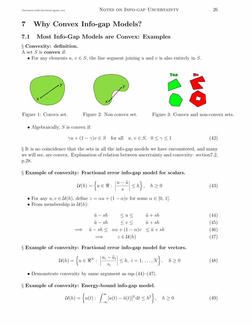
§ Convexity: definition.A set S is convex if:• For any elements u, v ∈ S, the line segment joining u and v is also entirely in S.

Figure 1: Convex set. Figure 2: Non-convex set. Figure 3: Convex and non-convex sets.

• Algebraically, S is convex if:

γu+ (1− γ)v ∈ S for all u, v ∈ S, 0 ≤ γ ≤ 1 (42)

§ It is no coincidence that the sets in all the info-gap models we have encountered, and manywe will see, are convex. Explanation of relation between uncertainty and convexity: section7.2,p.28.

§ Example of convexity: Fractional error info-gap model for scalars.

U(h) ={u ∈ < :

∣∣∣∣u− us∣∣∣∣ ≤ h

}, h ≥ 0 (43)

• For any u, v ∈ U(h), define z = αu+ (1− α)v for some α ∈ [0, 1].• From membership in U(h):

u− sh ≤ u ≤ u+ sh (44)

u− sh ≤ v ≤ u+ sh (45)

=⇒ u− sh ≤ αu+ (1− α)v ≤ u+ sh (46)

=⇒ z ∈ U(h) (47)

§ Example of convexity: Fractional error info-gap model for vectors.

U(h) ={u ∈ <N :

∣∣∣∣ui − uisi

∣∣∣∣ ≤ h, i = 1, . . . , N}, h ≥ 0 (48)

• Demonstrate convexity by same argument as eqs.(44)–(47).

§ Example of convexity: Energy-bound info-gap model.

U(h) ={u(t) :

∫ ∞−∞

[u(t)− u(t)]2 dt ≤ h2}, h ≥ 0 (49)


• For any u(t), v(t) ∈ U(h), define z(t) = αu(t) + (1 − α)v(t) for any α ∈ [0, 1]. We mustshow that z(t) ∈ U(h).• We see that:

z(t)− u(t) = α [u(t)− u(t)]︸︷︷︸x(t)

+(1− α) [v(t)− u(t)]︸︷︷︸y(t)

(50)

which defines x(t) and y(t). Thus:∫ ∞−∞

[z(t)− u(t)]2 dt = α2∫x2 dt+ 2α(1− α)

∫xy dt+ (1− α)2

∫y2 dt (51)

• By the Cauchy-Schwarz inequality:

∫xy dt ≤

√∫x2 dt

√∫y2 dt (52)

• Because u(t), v(t) ∈ U(h) we see that:∫x2 dt ≤ h2 and

∫y2 dt ≤ h2 (53)

• Thus eq.(51) becomes:∫ ∞−∞

[z(t)− u(t)]2 dt ≤ α2h2 + 2α(1− α)h2 + (1− α)2h2 = [α + (1− α)]2h2 = h2 (54)

• Thus z(t) ∈ U(h) which proves that the set is convex.

§ Example of convexity: info-gap model of a pdf.

U(h) ={p(x) : p(x) ≥ 0,

∫ ∞−∞

p(x) dx = 1, |p(x)− p(x)| ≤ p(x)h}, h ≥ 0 (55)

• For any p(x), q(x) ∈ U(h), define z(x) = αp(x) + (1− α)q(x) for some α ∈ [0, 1].• Clearly z(x) ≥ 0. Also:∫ ∞

−∞z(x) dx = α

∫ ∞−∞

p(x) dx+ (1− α)∫ ∞−∞

q(x) dx = 1 (56)

• Finally:

(1− h)p(x) ≤ p(x) ≤ (1 + h)p(x) (57)

(1− h)p(x) ≤ q(x) ≤ (1 + h)p(x) (58)

=⇒ (1− h)p(x) ≤ αp(x) + (1− α)q(x) ≤ (1 + h)p(x) (59)

• Hence z(x) ∈ U(h).


7.2 Why Are Most Info-Gap Models Convex?

¶ One explanation/motivation for convex info-gap models:1. Macroscopic events result from superposition of many microscopic events.2. Superpositions of many microscopic events tend to cluster convexly.

¶ We can understand this by analogy to the central limit theorem:

Given i.i.d. random variables x1, x2, . . . with mean µ and finite variance σ2.The distribution of x1, x2, . . . is arbitrary.The xi may be either discrete or continuous.Define the n-fold linear superposition:

Sn =1

σ√n

n∑i=1

(xi − µ) (60)

The distribution of Sn converges asymptotically to a standard normal distribution,regardless of the distribution of x1, x2, . . .:

limn→∞

Snprob= N (0, 1) (61)

Interpretation:Linear superposition of many arbitrarily distributed random variablesconverges to a specific macroscopic distribution: normal.

¶ Now consider the following info-gap-analog of the central limit theorem:

Let X be an arbitrary set (not necessarily convex).Define the n-fold linear superposition:

ξn =1

n

n∑i=1

xi for xi ∈ X (62)

Consider the set of all such n-fold superpositions:

Sn =

{ξ : ξ =

1

n

n∑i=1

xi for all xi ∈ X}

(63)

Sn is not convex unless X is convex.However, the sequence of sets S1, S2, . . .converges to a convex set:

limn→∞

Sn = ch(X ) (64)

Interpretation: Superposition of many arbitrary microscopic events of arbitrary dispersiontends to a convex cluster.Interpretation: Under deep uncertainty we cannot exclude any linear combination of events.Thus deep uncertainty induces convex-set representation.

Lecture Notes on Info-Gap Uncertainty - Technion

Documents

Transcript of Lecture Notes on Info-Gap Uncertainty - Technion