Lecture Notes on Economics of Financial Risk...
85
Lecture Notes on Economics of Financial Risk Management 1 Xiaodong Zhu 2 March 20, 2011 1 Incomplete draft for class uses only. Please do not circulate or cite without the author’s permission. 2 Professor, Department of Economics, University of Toronto. Email: [email protected]
Transcript of Lecture Notes on Economics of Financial Risk...

Lecture Notes on Economics of Financial Risk
Management1
Xiaodong Zhu2
March 20, 2011
1Incomplete draft for class uses only. Please do not circulate or cite without the
author’s permission.2Professor, Department of Economics, University of Toronto. Email:

2

Chapter 1
Introduction
This course is about financial risk management. We will focus our discussionon why, when and where there is a need for risk management and how tomeasure and manage risk.
According to the Webster’s New World Dictionary, risk is the chance ofinjury, damage, or loss. By this definition, humankind has always faced andhad to deal with many kinds of risk such as war, famine, deadly diseases, badweather, theft, robbery, etc..Ideally, we would hope that we can eliminatethe sources of risk so that we can live in a risk-free world. There has beensome progress towards this goal. For example, most developed countrieshave almost certainly eliminated the possibility of famine. However, we arestill living in a world that is far from risk-free. Despite enormous progressin many aspects of our daily life in the last few hundred years, risk is stilleverywhere in our life. A few examples:
• A firm may be taken over by another firm and its workers may be laidoff.
• An earthquake or hurricane may hit a city.
• An electricity blackout may happen to a large region.
• A student may not be able to find a good job upon graduation.
• Your computer may be infected by a deadly virus or worm.
• Weather may be unexpectedly bad.
• Stock market may crash
3

4 CHAPTER 1. INTRODUCTION
• Tuition may increase
• US dollar may devalue dramatically against the Euro
When risk cannot be eliminated, the best way to deal with it is sharing itbetween lucky and unlucky ones. A major role of financial markets is tofacilitate more efficient risk sharing among individuals, firms and govern-ments. Financial innovations often occur to deal with new kinds of risk or toprovide new ways to deal with old risk. Over the last three decades, finan-cial innovations have been occurring at a frantic pace. Many new financialinstitutions, markets and products have been created. Markets for deriva-tives, in particular, exploded in the late 1980s and early 1990s. By 2001, thenotional value of all derivatives outstanding amounted to $111 trillion. Incomparison, the world GDP was only $31.3 trillion, and the capitalizationof the stock markets of the industrialized countries was $21.2 trillion. Theexplosive growth in derivatives has made many people rich, and the marketattracted talented individuals with very different backgrounds. Many Ph.D.sin economics, geophysics, chemical engineering, mathematics, computer sci-ence and other fields went to work on Wall Street. New professional programsin Mathematical Finance, Financial Engineering or Computational Financehave also been created in many universities.
With all the new derivatives that were invented or re–invented, one wouldexpect that we should be much better at managing risk. Yet, today we stillcan not effectively manage many of the risk mentioned in the examples above.In the meantime, we heard all these news about spectacular losses associatedwith trading derivatives: Barings Bank, Orange County Government, Pocterand Gamble, Long Term Capital Management, etc. How does financial inno-vation help us to manage risk? Does financial innovation help us to managerisk? Could financial innovation create risk? What causes financial innova-tion? Should the society limit financial innovation? These are the centralquestions that we will try to address. To put things in perspective, it is usefulto first take a brief look at the history of financial innovation.
1.1 A Brief History of Financial Innovation
Financial innovation is not a new phenomenon. Probably the earliest andone of the most important financial innovation is personal loan. A loan fromone person to another can help both people to share risk and smooth their

1.1. A BRIEF HISTORY OF FINANCIAL INNOVATION 5
income and expenditures over time. There is evidence that loans were usedin many ancient civilizations. Banks that took deposits and lent money wereestablished in Babylonia, Assyria and ancient Greece. They helped people toshare risk and smooth their income and expenditures at a much larger scale.
Equities were issued by joint stock companies during the sixteenth cen-tury. Owners of equities could be those who work in the company or someonewho simply provided financial capital. Issuing equities to “sleep partners”who did not actively involve in day–to–day operations allowed separation ofownership and control. This was very important because it allowed profitand risk sharing between those who knew how to produce and those whohad money.
Bonds were first used by European governments in the sixteenth cen-tury. Collecting taxes was costly and time consuming, and it could be verydisruptive to the economy if a government had to finance all of its war ex-penditures by levying a very high tax during the wartime. To smooth thetax burden overtime, governments often financed their war expenditures byissuing bonds to the public. Today governments are still the biggest playersin the bond market.
Initially, equities and bonds were mainly held by corporate insiders andwealthy investors. As the total amount of these securities became larger,more investors were needed to share the risk. This gave rise to secondarytrading, first informally on the streets, latter in organized exchanges. Thefirst exchange was the Amsterdam Stock Exchange opened in 1611, then thestock exchange in London in 1802 and New York Stock exchange in 1817(known as New York Stock and Exchange Board then). Commodity futuresexchanges emerged in Chicago in the 19th century. In the 1840s, Chicagobecame the commercial center for the Midwestern farm states. (The name ofthe basketball team Chicago Bulls originated from the fact that Chicago wasa main distributor of beef in those days.) To make the trading of agricultureproducts more efficient, the Chicago Board of Trade (CBOT) was establishedin 1848. The establisher’s original purpose was to standardize the quantitiesand qualities of the grain being traded. However, contracts for the futuredelivery of grain started to trade soon after the establishment of the exchange.These allowed producers and processors to share the risk of fluctuations inprices.
The development of markets for financial derivatives is more recent. Fi-nancial futures and options on foreign exchange and interest rates were intro-duced and traded in the early 1970, and the futures on stock market indices

6 CHAPTER 1. INTRODUCTION
were introduced in the early 1980s. The financial innovation in this periodis a response to the increasing volatility in the financial markets. There arethree main reasons for the increasing volatility: (1) The oil crises in the early1970s and early 1980s that directly and indirectly resulted in the significantdrops in the stock prices and increases in commodity price volatility. (2)The increased inflation and interest rate risk. (3) The breakdown of BrettonWoods System and the end of fixed exchange rates for most industrializedcountries.

Chapter 2
Arrow-Debreu Theory of
Financial Markets
In discussing uncertainty and risk, two concepts are very important: statesof nature and state contingent plan (contingent means depending on someoutcome that is not yet known), which we define below:
• states of nature, which refer to different outcomes of some randomevent and
• state contingent plan, which specifies how much to be consumed(consumption plan), how much income to have (income plan), or whatpayoff to have (payoff plan) in each state of nature.
Example 1. Consider someone who has $100 and is considering whether tobuy a Number 13 lottery ticket or not. The cost of the ticket is $5, and thewinner receives $200. In this example, there are two states of nature: (1)number 13 is drawn and (2) number 13 is not drawn. If the individual doesnot buy the lottery ticket, then her plan is to have $100 in both states, whichcan also represented by a two-dimensional vector (100, 100). Here the firstelement of the vector represents the individual’s income in the state whennumber 13 is drawn and the second element the individual’s income in theother state. If the individual buys the ticket, then, her plan is
{295 number 13 is drawn,95 number 13 is not drawn.
7

8CHAPTER 2. ARROW-DEBREU THEORY OF FINANCIAL MARKETS
Alternatively, we can represent the plan as (295, 95). We can also representthe payoffs of the lottery ticket as a payoff plan
Lottery ticket=
{200 number 13 is drawn,0 number 13 is not drawn.
or simply (200, 0).
Example 2. Consider someone who has $35,000 initial wealth. There isa possibility that an accident will occur such that the individual will lose$10,000, maybe as a result of car accident or fire in the house. In this example,the two states of nature are" there is an accident" and "no accident". Theindividual’s wealth in this example is also a state-contingent plan:
{25, 000 there is an accident,35, 000 no accident,
or (25000, 35000). The individual can change her wealth plan by buying aninsurance plan. Consider an insurance plan that pays K dollars in the stateof accident costs 0.01K dollars. If the individual buys the insurance plan,then her wealth after insurance would be
{25, 000 +K − 0.01K there is an accident,
35, 000− 0.01K no accident
or (25000+ 0.99K, 35000− 0.01K). For example, if the individual pays $100in both states of nature (K = 10, 000), then she will get $10,000 from theinsurance in the state when there is an accident and nothing when there isno accident. As a result, the individual’s wealth after insurance would be
{34, 900 there is an accident,34, 900 no accident
or (34900, 34900). We can graph all the feasible wealth plans the individualcan have through insurance in Figure 1. Note that in the graph, we allow forthe possibility that the amount of insurance K to be negative. That is, theindividual can have consumption plans under which she consumes less than$25,000 in the state of accident. In such cases, the individual is effectivelyshort or selling insurance.
In both Example 1 and 2, we consider the cases when there are onlytwo possible states, so any state contingent plan can be represented by a

9
two-dimensional vector. Similarly, for any positive integer N , if there areN possible states, we can also represent a state contingent plan by an Ndimensional vector. (See the appendix at the end of this chapter for a briefintroduction to vectors and linear algebra.) So, a consumption plan can berepresented by a vector (c1, c2, ..., cN), where ci is how much to be consumedif the ith state is realized.
A financial security can also be represented by a vector a = (a1, ..., aN),where ai is the security’s payoff in state i for i = 1, ..., N . For example,(1, ..., 1) represents a risk–free security that pays one unit of good in everystate, and (−1,−1, ..., 2, 2) a risky security that has negative payoffs in somestates and positive payoffs in some other states.
Definition The financial market is complete if all financial securities canbe traded. That is, for any arbitrary N numbers a1, ..., aN , a security withpayoff plan a = (a1, ..., aN) can be bought or sold in the market.
We denote the price of a security a by P (a). For any two securitiesa = (a1, ..., aN) and b = (b1, ..., bN), a third security can be formed by aportfolio of these two securities: αa + βb, where α and β are any two realnumbers. If α (or β) is a negative number, then the portfolio includes short–selling (which means selling a security without actually owning it) ratherthan holding security a (or b). There is no arbitrage in the financial marketif for any α and β, we have
P (αa+ βb) = αP (a) + βP (b) (2.0.1)
That is, if the payoff of a security can be replicated by a portfolio of someother securities, then the price of this security (P (αa + βb)) should be thesame as the cost of forming the portfolio (αP (a) + βP (b)).
In the rest of this chapter, we will always assume that there is no-arbitrageunless stated otherwise.
Theoretically, it is useful to think of the following basic securities,
b(1) = (1, 0, ..., 0)b(2) = (0, 1, ..., 0)
......b(N) = (0, ..., 0, 1)
Here, b(i) is the security that pays one unit in state i and nothing in anyother states.

10CHAPTER 2. ARROW-DEBREU THEORY OF FINANCIAL MARKETS
Note that Any security a = (a1, ..., aN) can be constructed as a portfolioof these basic securities:
a = a1b(1) + ...+ aNb(N).
Therefore, the market is complete if these basic securities and the portfoliosof these basic securities can be traded in the market. Under the no-arbitragecondition, then, we have
P (a) = a1P (b(1)) + ...+ aNP (b(N)). (2.0.2)
In the real world, securities that are traded are usually not basic secu-rities. To determine whether the market is complete or not, then, all weneed to know is whether the basic securities can be replicated by portfoliosof securities that are traded in the market.
Example 3. There are only two states. There are two securities that aretraded in the market: a risk–free bond B = (1, 1) and a risky stock A = (1, 2).Then, the basic securities can be formed as follows:
b(1) = 2B − A = (1, 0)b(2) = A− B = (0, 1)
that is, b(1) can be replicated by holding two units of B and short–selling oneunit of A, and b(2) can be replicated by holding one unit of A and short–sellingone unit of B. Thus, the market is complete in this example.
Example 4. There are three states. Again, there are two securities thatare traded in the market: a risky stock A = (1, 2, 3) and a risk–free bondB = (1, 1, 1). In this example, the market is not complete since no portfolioof A and B can replicate the basic security b(1). To see this, let αA+ βB bea portfolio that replicates the payoff of b(1) in the first two states, that is
α+ β = 1,2α+ β = 0,
which implies that α = −1 and β = 2. The payoff of this portfolio in thethird state, then, is −1× 3 + 2× 1 = −1, which is different from zero payoffof b(1). So, there exists no combination of α and β such that αA+ βB = b1.

11
Remark: Example 4 is a special example of a more general property: Fora market to be complete in an economy with N states, there should be at leastN securities traded in the market that have linearly independent payoffs (i.e.,the matrix that is formed by stacking the N securities’ payoffs is invertibleor nonsingular).
Example 5. The same environment as in example 4 except that derivativesecurities based on A can be traded now. In this case, the basic securityb(3) can be replicated by an option on the stock A. Let C be the option onA with strike price 2. That is, the holder of the option has the right, butnot obligation, to buy one unit of A with price 2 in any states. Apparently,the holder would buy the stock only in the state in which the payoff of A isgreater than 2, which is the third state. Thus, the payoff of the option is
C = max{A− 2, 0} = (0, 0, 1) = b(3).
With the new security C, then, the basic securities can be replicated asfollows:
b(1) = 2B − A+ C,b(2) = A−B − 2C,b(3) = C.
Thus, the originally incomplete market is completed with trading of options.
Appendix: Linear Algebra
2.0.1 Some Basic Definitions
Matrix–an array of numbers:
A ≡ [aij ]m×n ≡
a11 a12 . . . a1na21 a22 . . . a2n. . . . . .. . . . . .. . . . . .
am1 am2 . . . amn
Examples:

12CHAPTER 2. ARROW-DEBREU THEORY OF FINANCIAL MARKETS
identity matrix
I =
1 0 . . . 00 1 . . . 0. . . . . .. . . . . .. . . . . .0 0 . . . 1
scalar matrix
c 0 . . . 00 c . . . 0. . . . . .. . . . . .. . . . . .0 0 . . . c
2.0.2 Matrix Operations
Sum and Multiplication by a Scalar:
A +B = [aij + bij ]
cA = [caij ]
some properties:
A+B = B + A
c (A+B) = cA+ cB
column vector
x =
x1
x2
.
.
.xn
row vectory′ =
[y1 y2 . . . yn
]

13
multiplication of vectors
y′x =n∑
k=1
ykxk
multiplication of matrices
A = [aij ]m×n , B = [bij ]n×p , C ≡ AB ≡ [cij]m×p
A =
a′(1)a′(2)...
a′(m)
, B =
[b1 b2 . . . bn
]
wherea′(i) =
[ai1 ai2 . . . ain
]
bj =
b1jb2j...bnj
cij = a′(i)b(j) =n∑
k=1
aikbkj.
Some Properties:(i) In general, AB 6= BA.(ii) IA = AI = A.(iii) Ax = x1a1 + ...+ xnan.
2.0.3 Inverse of a Matrix
Vectors a1, ..., an are linearly independent if and only if none of them can bewritten as a linear combination of the others. Equivalently,
x1a1 + ...+ xnan = 0 =⇒ x1 = ... = xn = 0.

14CHAPTER 2. ARROW-DEBREU THEORY OF FINANCIAL MARKETS
Proof: if one of the xi’s is not zero, say x1 6= 0, then
a1 = x−11 x2a2 + ...+ x−1
1 xnan,
which is contradictory to the assumption.
A square matrix A is nonsingular or invertible if there exists a squarematrix B such that
AB = BA = I, B ≡ A−1.
(i) If A is nonsingular, then its column vectors are linearly independent.
Ax = 0 =⇒ A−1 (Ax) =(A−1A
)x = x = 0.
(ii) If A is nonsingular, then equation Ax = y has a unique solution.
Ax = y =⇒ A−1 (Ax) = A−1y =⇒ x = A−1y.
(iii) If A is nonsingular, then the determinant of A is nonzero, det(A) 6= 0
2.0.4 Determinant of a Matrix
For a two dimensional matrix,
A =
[a bc d
]
we havedet(A) = ad− cb
For a three dimensional matrix, if it has the following form:
A =
a b ec d f0 0 g
then, we have
det(A) = det
([a bc d
])× g

Chapter 3
Applications of Arrow-Debreu
Theory: Pricing Options
Even though Arrow-Debreu Theory is an abstract economic theory, it hasvery practical applications in finance. In this section we illustrate the use-fulness of this theory by showing how it can be used for pricing options andother derivative contracts.
3.1 Pricing Options in a Simple Two-State Econ-
omy
A financial market is open now (time zero) for trading securities that paysoff at some time in the future. The length of the time period between nowand the payoff date is ∆t. In finance, we always use year as the unit of time.So ∆t = 1,1/2,1/4, and 1/12 represent one year, half a year, a quarter and amonth, respectively. There are two securities that are traded in the market:A is a stock and B is a bond. The price of the stock today is S (S > 0) andthe price of the bond today is 1. There are two possible states of nature at∆t, and the stock’s value is state-contingent. It will equal SD in the firststate and SU in the second state, where D and U are two constants suchthat 0 < D < 1 < U . So, the first state is the state when the stock price goesdown (because SD < S), and the second state is the state when the stockprice goes up (because SU > S). In contrast, the value of the bond at time∆t will be eR∆t in both states of nature. Here R is the annualized risk-freeinterest rate. Figure 2 is a graphical representation of the two assets.
15

16CHAPTER 3. APPLICATIONS OF ARROW-DEBREU THEORY: PRICING OPTIONS
We can represent the two assets using the Arrow-Debreu language: A =(SD, SU), B = (eR∆t, eR∆t), P (A) = S and P (B) = 1. It is clear that A andB are not proportional to each other. That is, they are linearly independent.Therefore, we know that the market is complete. In particular, the two basicsecurities, b(1) = (1, 0) and b(2) = (0, 1) can be replicated by portfolios of Aand B.
Using Stock and Bond Prices to Find the Prices of the Basic Se-
curities
Let’s first see how we can form a portfolio of A and B, α1A+ β1B, suchthat its payoffs are the same as b(1). In other words, we are looking for α1
and β1 such that
α1SD + β1eR∆t = 1, (3.1.1)
α1SU + β1eR∆t = 0. (3.1.2)
Subtracting (3.1.2) from (3.1.1) yields the following:
α1S(D − U) = 1
which implies that
α1 =1
S(D − U)= − 1
S(U −D).
Substituting the equation above into (3.1.2), we have
− 1
S(U −D)SU + β1e
R∆t = 0
or
β1eR∆t =
U
U −D,
which implies that
β1 =e−R∆tU
U −D.
Thus, we have
b(1) = − 1
S(U −D)A+
e−R∆tU
U −DB. (3.1.3)

3.1. PRICING OPTIONS IN A SIMPLE TWO-STATE ECONOMY 17
Similarly, to find the portfolio of A and B, α2A+β2B, that replicates thepayoffs of b(2), we solve the following equations:
α2SD + β2eR∆t = 0, (3.1.4)
α2SU + β2eR∆t = 1. (3.1.5)
Subtracting (3.1.4) from (3.1.5) yields the following:
α2S(U −D) = 1
which implies that
α2 =1
S(U −D).
Substituting the equation above into (3.1.4), we have
1
S(U −D)SD + β2e
R∆t = 0
or
β2eR∆t = − D
U −D,
which implies that
β2 =e−R∆tD
U −D.
Thus, we have
b(2) =1
S(U −D)A− e−R∆tD
U −DB. (3.1.6)
From equation (3.1.3) and (3.1.6) we can determine the prices of b(1) andb(2) using the non-arbitrage equation in Chapter 2, (2.0.1). Thus, we have
P (b(1)) = α1P (A) + β1P (B)
= − 1
S(U −D)S +
e−R∆tU
U −D
or
P (b(1)) =e−R∆tU − 1
U −D. (3.1.7)
Similarly,
P (b(2)) = α2P (A) + β2P (B)
=1
S(U −D)S − e−R∆tD
U −D

18CHAPTER 3. APPLICATIONS OF ARROW-DEBREU THEORY: PRICING OPTIONS
or
P (b(2)) =1− e−R∆tD
U −D. (3.1.8)
No-Arbitrage Constraints on Basic Security Prices
Since both basic securities pay off a positive amount in one state andnothing in the other state, the prices of these two securities have to be pos-itive. Otherwise, everyone would want to buy an infinite amount of thesesecurities and the market would not be cleared. So, to be consistent withno-arbitrage, we need the following conditions to hold:
P (b(1)) =e−R∆tU − 1
U −D> 0
P (b(2)) =1− e−R∆tD
U −D> 0
The first condition requires that e−R∆tU > 1, or U > eR∆t, and the secondcondition requires that e−R∆tD < 1, or D < eR∆t. That is, no-arbitragerequires the following to be true:
D < eR∆t < U . (3.1.9)
Intuitively, the conditions are that the risk free return on bond has to behigher than the lowest possible return on stock (otherwise nobody wouldbuy bond) and lower than the highest possible return on stock (otherwisenobody would buy stock).
Using the Basic Security Prices to Price All Securities
For any security in the market, a = (a1, a2), we can write it as a portfolioof the two basic securities:
a = a1b(1) + a2b(2).
Again, using the non-arbitrage equation in Chapter 2, (2.0.1), we have
P (a) = a1P (b(1)) + a2P (b(2)). (3.1.10)
From (3.1.7) and (3.1.8), then, we have
P (a) =e−R∆tU − 1
U −Da1 +
1− e−R∆tD
U −Da2.

3.1. PRICING OPTIONS IN A SIMPLE TWO-STATE ECONOMY 19
Example 6. S = 100, U = 1.1, D = 0.9, R = 0, ∆t = 1. That is, the payoffsof the stock are (90, 110), and the payoffs of the bond are (1, 1). Then,
P (b(1)) =e−R∆tU − 1
U −D=
e−0x11.1− 1
1.1− 0.9=
0.1
0.2=
1
2,
P (b(2)) =1− e−R∆tD
U −D=
1− e−0x10.9
1.1− 0.9=
0.1
0.2=
1
2.
For a call option on stock (i.e., the option to buy stock) with strike price (orexercise price) 100, the option payoff is 0 when the stock price is 90 and 10when the stock price is 110. So, a = (0, 10) and the option price is given by
P (a) =1
2× 0 +
1
2× 10 = 5.
For a put option on stock (i.e., the option to sell the stock) with strike price(or exercise price) 100, the option payoff is 10 when the stock price is 90 and0 when the stock price is 110. So, a = (10, 0) and the option price is givenby
P (a) =1
2× 10 +
1
2× 0 = 5.
Example 7. The same as in example 6 except that R = 0.05. Then,
P (b(1)) =e−R∆tU − 1
U −D=
e−0.05×11.1− 1
1.1− 0.9= 0.232,
P (b(2)) =1− e−R∆tD
U −D=
1− e−0.05x10.9
1.1− 0.9= 0.719.
So, the price of the call option on stock with strike price 100 is
P (a) = 0.232× 0 + 0.719× 10 = 7.19,
and the price of the put option on stock with with strike price 100 is
P (a) = 0.232× 0 + 0.719× 0 = 2.32.
Note that as the interest rate increases from 0 to 0.05, the price of call optionrises and the price of the put option declines.

20CHAPTER 3. APPLICATIONS OF ARROW-DEBREU THEORY: PRICING OPTIONS
Example 8. The same as in example 6, but now consider a security whosepayoff is the stock price squared. So, a1 = 902 = 8100, and a2 = 1102 = 12100
P (a) =1
2× 8100 +
1
212100 = 10100.
The security that we consider in this example may look unusual. However,many unusual or exotic derivative contracts have in fact been traded in prac-tice.
Example 9. The same as in example 6, but now consider a forward contract,i.e. a contract to buy the stock at a fixed price of 100. Note that the forwardcontract differs from the option contract in that the holder of the contracthas to buy the stock. So, a = (−10, 10) and the price of the forward contractis
P (a) =1
2× (−10) +
1
2× 10 = 0.
If the interest rate is 0.05, as in example 7, then,
P (a) = 0.232× (−10) + 0.719× 10 = 4.87.
Risk-Neutral or Risk-Adjusted Probabilities
From equation (3.1.9) we can see that to price securities, all we need toknow are the state-contingent payoffs of the securities and the prices of thetwo basic securities, P (b(1)) and P (b(2)), which themselves are derived fromthe prices of the stock and bond traded in the market. This is somewhatsurprising. For example, the basic security b(1) pays one dollar in state oneand nothing in the second state. One would think that the price of thissecurity should depend on how likely it is that the state one will be realizedas well as how much investors value having one dollar in state one. Yet, whenwe derive the price of the security, we did not use any such information. Onlyinformation on stock and bond prices are used. This is possible because underno-arbitrage condition, financial market is efficient and therefore the marketprices of stocks and bonds have already contained all the information that isneeded for pricing any securities.
There is, however, a probabilistic representation of the pricing of securi-

3.1. PRICING OPTIONS IN A SIMPLE TWO-STATE ECONOMY 21
ties. Let
q =P (b(1))
P (b(1)) + P (b(2))=
U − eR∆t
U −D, (3.1.11)
1− q =P (b(2))
P (b(1)) + P (b(2))=
eR∆t −D
U −D. (3.1.12)
Under the no-arbitrage condition (3.1.9), we know that 0 < q < 1. So both qand 1− q can be thought of as probabilities. From the construction, we have
P (b(1)) =[P (b(1)) + P (b(2))
]q, (3.1.13)
P (b(2)) =[P (b(1)) + P (b(2))
](1− q). (3.1.14)
From the equations for basic security prices that we derived earlier, (3.1.7)and (3.1.8), we have
P (b(1))+P (b(2)) =e−R∆tU − 1
U −D+1− e−R∆tD
U −D=
e−R∆tU − e−R∆tD
U −D=
e−R∆t(U −D)
U −D.
So,P (b(1)) + P (b(2)) = e−R∆t
Substituting it into (3.1.11) and (3.1.12) yields the following
P (b(1)) = e−R∆tq,
P (b(2)) = e−R∆t(1− q).
Therefore, for any security a = (a1, a2), from equation (3.1.10), we have
P (a) = e−R∆tqa1 + e−R∆t(1− q)a2 = e−R∆t [qa1 + (1− q)a2] . (3.1.15)
If we think of q and 1 − q as the probabilities of state one and two,respectively, then qa1+(1−q)a2 is simply the expected value of the security’spayoffs, and equation (3.1.15) says that the price of the security equals theexpected payoff discounted by the risk-free interest rate. In other words,under these probabilities, we price a security as if we are risk neutral–allwe care about is the expected payoff. For this reason, we call q and 1 − qthe risk-neutral probabilities. This, however, does not mean that investorsare risk-neutral. The risk-neutral probabilities are in general not the sameas investors’ subjective probabilities. They are related to the subjectiveprobabilities, but adjusted for the risk attitudes that investors have. We willgo back to this point in more detail in the next chapter.

22CHAPTER 3. APPLICATIONS OF ARROW-DEBREU THEORY: PRICING OPTIONS

Chapter 4
Individual and Social Gains from
Risk Management
4.1 Individual’s Attitude Towards Risk
In the economy with risky outcomes, individuals’ consumption may be statedependent. Let ci be an individual’s consumption in state i, for i = 1, ..., Nand let c = (c1, ..., cN) be the individual’s consumption plan. The individual’spreference over different consumption plans is represented by an expectedutility function
U(c) = E[u(c)] = π1u(c1) + ...+ π(sN)u(cN),
where πi is the subjective probability that state i will be realized. In thischapter, we assume that all individuals share the same belief and have thesame subjective probabilities of states. So, πi can also be thought of as the“objective” probability that state i will be realized.
We call an individual risk–averse if for any two consumption plans, ca =(ca1, ..., c
aN) and cb = (cb1, ..., c
bN) that have the same expected consumption
level, i.e.π1c
a1 + ...+ πNc
aN = π1c
b1 + ...+ πNc
bN ,
she prefers the one with lower variance. If an individual is indifferent be-tween any two alternative consumption plans that have the same expectedconsumption level, then we call her risk–neutral.
An individual’s risk attitude is related to the curvature of her utilityfunction u(.). If an individual’s utility function is linear, then she only cares
23

24CHAPTER 4. INDIVIDUAL AND SOCIAL GAINS FROM RISK MANAGEMENT
about the expected consumption level and, therefore, is risk–neutral. If anindividual’s utility function is concave, i.e. u′′(x) < 0 for any x, then theindividual is risk-averse. By Jensen’s inequality1,
U(c) = E[u(c)] ≤ u(E[c]),
where E[c] = π1c1 + ... + πNcN is the expected consumption level, and theequality holds if and only if ci = E[c] for all i = 1, ..., N . Thus, a risk–averse individual strictly prefers to have a risk–free consumption plan (i.e.,consumption does not vary across states) over any risky consumption plan(i.e., consumption varies across at least two different states). If her incomeis risky and if it is possible, she would trade her risky income for a risk–free consumption plan that allows her to consume her expected income inevery states. In fact, she is willing to trade for a risk–free consumption planthat allows her to consume at a level that is below her expected income. Inother words, she is willing to pay a positive risk–premium, measured by thereduction in her expected consumption, in order to eliminate the income risk.
Insert Figure 3 Here
Figure 3 illustrates the benefits of eliminating income risk for a risk–averseindividual and the maximum risk–premium she is willing to pay. Consideran economy with two possible states, {s1, s2}. The individual’s income inthe two states are yl and yh, respectively, where yh > yl. So s1 can bethought of as the bad state and s2 the good state for the individual. Theindividual’s utility function is plotted in the figure as u(.). If the individualsimply consumes her income, then she has a high level of consumption in thegood state but a low level of consumption in the bad state. The expectedutility of such a consumption plan is
π1u(yl) + π2u(yh),
1Jensen’s Inequality refers to the following mathematical proposition: If a function,f(.), is concave (i.e., f ′′(x) < 0 for any x), then,
n∑
i=1
αif(xi) ≤ f
(n∑
i=1
αixi
)
for any positive integer n, and any α1 > 0,...,αn > 0 such that∑
n
i=1αi = 1. Furthermore,
the equality holds if and only if x1 = x2 = ... = xn.

4.2. INDIVIDUAL DEMAND FOR RISK MANAGEMENT 25
which is represented graphically by the height of point A. If the individualtrades her risky income for a risk–free consumption plan, (x, x), then theexpected utility of such a consumption plan is π1u(x) + π2u(x) = [π1 +π2]u(x) = u(x), which is graphically represented by the height of the utilityfunction u(.) evaluated at x. If x = E[y] ≡ π1yl + π2yh, then the expectedutility she enjoys is represented by the height of point A′, which is higher thenpoint A. The lowest level x that the individual is willing to trade for is x∗ atwhich the individual’s expected utility is the same as that from consumingher own risky income. The distance between E[y] and x∗, E[y]− x∗, is themaximum risk–premium or the reduction in the expected consumption level,that the individual is willing to pay for eliminating her income risk. Whethershe will be able to trade at such a risk premium depends how risk–averse otherindividuals in the economy are and whether the individual’s income risk isdiversifiable or not. In the next section, we will examine the conditions underwhich individuals will be able to trade financial securities to reduce the riskthey face.
4.2 Individual Demand for Risk Management
Consider now an Arrow-Debreu economy that consists of M individuals, in-dexed by j = 1, ...,M . Each individual’s income is state-contingent. For anyi = 1, ..., N and j = 1, ...,M , let yj,i be individual j’s income in state i. So,individual j’s income over all possible states can be represented by a vectory(j) = (yj,1, ..., yj,N). The individual’s problem is to choose a consumptionplan, c(j) = (cj,1, ..., cj,N), which determines the amount of consumption ineach possible state, in order to maximize his/her expected utility function:
U(c(j)) = E[c(j)] = π1uj(cj,1) + ...+ πNuj(cj,N).
For simplicity, we assume that individuals’ utility function is of the followingform:
uj(c) =1
1− γj[c1−γj − 1], γj ≥ 0.
Remember that the relative risk aversion coefficient of a utility function isgiven by RRAC = −u′′(c)c/u′(c) and it measures the degree of risk aversionof an individual with utility function u(.). For the utility function specifiedabove, RRAC = γj, which is a constant. So, the utility functions of thisform are also called constant relative risk aversion utilities. The parameter

26CHAPTER 4. INDIVIDUAL AND SOCIAL GAINS FROM RISK MANAGEMENT
γj represents the degree of individual j’s risk–aversion. The larger is γj , themore risk–averse individual j is. If γj = 0, individual j is risk–neutral; ifγj > 0, individual is risk averse; and if γj < 0, individual is risk loving.
We assume that the market is complete and individuals trade financialsecurities in order to achieve their optimal consumption plans. Individual j’sconsumption plan can be accomplished if she can buy a portfolio that payscj,i in state i for all i = 1, ..., N . From the no-arbitrage equation, we knowthat the cost of such a portfolio is
cj,1p1 + ...+ cj,NpN .
The individual can finance its consumption plan by selling its income port-folio, which has value
yj,1p1 + ...+ yj,NpN .
So, the individual’s problem is
maxcj,1,...,cj,N
1
1− γj
N∑
i=1
πi
[c1−γjj,i − 1
]
subject to the budget constraint
N∑
i=1
cj,ipi ≤N∑
i=1
yj,ipi.
Define a Lagrangian Lj as follows:
Lj =1
1− γj
N∑
i=1
πi
[c1−γjj,i − 1
]+ λj
[N∑
i=1
yj,ipi −N∑
i=1
cj,ipi
].
Then, the individual’s optimal consumption plan is determined by the fol-lowing first order conditions:
∂Lj
∂cj,i= πic
−γjj,i − λjpi = 0, for i = 1, ..., N. (4.2.1)
The individual’s optimal consumption plan is the solution to equation (4.2.1)and the following complementarity conditions:
λj ≥ 0, and λj
[N∑
i=1
yj,ipi −N∑
i=1
cj,ipi
]= 0

4.2. INDIVIDUAL DEMAND FOR RISK MANAGEMENT 27
From equation (4.2.1), we know that λj > 0. Thus, the above complemen-tarity condition implies that
N∑
i=1
cj,ipi =
N∑
i=1
yj,ipi, (4.2.2)
or the individual’s budget constraint is binding.From the first order condition (4.2.1), we can solve for the optimal con-
sumption demand of a risk-averse individual j (γj > 0), cj,i,
cj,i = λ−1/γjj
(πi
pi
)1/γj
= wjx1/γji , (4.2.3)
where wj = λ−1/γjj and xi = πi/pi. Equation (4.2.3) is a key equation for
understanding the role of financial market in managing individuals’ incomerisk. Without fully solving the model, we can already derive from the equa-tion some important implications of risk-sharing under a complete financialmarket.
Implication 1: A complete financial market allows individuals to
diversify all idiosyncratic income risks.
Note that xi is a variable that varies across states but does not dependon individual types. We can interpret it as a variable that represents theaggregate risk that is faced by every individual in the economy. Since wj
is a state-independent constant, equation (4.2.3) shows that each individ-ual’s consumption exposure to risk is entirely through the aggregate riskvariable xi. Therefore, any individual income risk that is uncorrelated withthe aggregate risk xi has no impact on consumption. In other words, witha complete financial markets, individuals can diversify away all idiosyncraticincome risks.
Implication 2: A complete financial market allows individuals to
share aggregate risk more efficiently.
Taking logarithm on both sides of equation (4.2.3), we have
ln cj,i = lnwj + γ−1j ln xi. (4.2.4)
Let σ2j and σ2
x be the variance of ln cj(si) and ln x(si), respectively, then
(4.2.4) implies that σ2j = γ−2
j σ2x or
σj
σj′=
γj′
γj

28CHAPTER 4. INDIVIDUAL AND SOCIAL GAINS FROM RISK MANAGEMENT
That is, the volatility of an individual’s optimal consumption is inverselyrelated to how risk–averse she is. Those who are highly risk–averse will endup having less risk in their consumption relative to those who are less risk–averse.
4.3 Equilibrium Prices of Arrow-Debreu Secu-
rities and Aggregate Risk
Since xi = πi/pi and pi is an endogenous variable, we need to solve forthe equilibrium value of pi to see how aggregate risk is determined in thiseconomy. In this section we present two special cases when we can solve xi
and pi explicitly.
Case 1: There exists some risk–neutral agents. Assume, for example,that individual 1 is risk–neutral, γ1 = 0. Then, she is willing to take anyincome risk as long as her expected consumption level is not reduced. As aresult, every risk–averse individual will completely eliminate her income riskby trading securities with the risk–neutral agent.2
For j = 1, equation (4.2.1) becomes
πi − λ1pi = 0
orpi = λ−1
1 πi. (4.3.1)
This implies that xi = λ1 for any i = 1, ..., N , and, from (4.2.3), for anyindividual j such that γj > 0,
cj,i = (λ1/λj)1/γj ≡ cj,
which is a constant across all N different states. From (4.2.2), then, we have,
cj
N∑
i=1
pi =
N∑
i=1
piyj,i.
2We assume that everyone in this economy is a price-taker. This is equivalent toassuming that there are many individuals for each type and there are perfect competitionamong them. If there is only one individual who is risk-neutral, the individual would havemonopoly power and therefore may charge a risk premium for taking income risk even ifshe is risk-neutral.

4.3. EQUILIBRIUM PRICES OF ARROW-DEBREU SECURITIES AND AGGREGATE RISK29
Substituting (4.3.1) into the equation above yields:
cj
N∑
i=1
λ−11 πi =
N∑
i=1
λ−11 πiyj,i,
or
cj = E[y(j)] =
N∑
i=1
πiyj,i.
So, the risk-averse individual j will choose to fully insure herself from incomefluctuations. The optimal consumption plan of individual j is
(E[y(j)], ..., E[y(j)]).
In other words, when there are risk–neutral agents in the economy, then allrisk–averse individuals can dump all of their income risk to the risk–neutralagents without paying any risk–premium.
Case 2: Individuals are equally risk–averse.
We assume that γj = γ for all j = 1, ...,M . Note that pi is the priceof (one unit of) consumption in state i. Like price of any commodity, pican be determined by the market clearing condition: Aggregate demand forconsumption in state i equals the aggregate income in the same state. From(4.2.3), the aggregate demand for consumption in state i is
Ci =
M∑
j=1
cj,i =
M∑
j=1
(wjx
1/γi
)=
(M∑
j=1
wj
)x1/γi .
Let Yi =∑M
j=1 yj,i be the aggregate income in state i. Then, the marketclearing condition implies that
Ci =
(M∑
j=1
wj
)x1/γi = Yi
or
xi =
(M∑
j=1
wj
)−γ
(Yi)γ . (4.3.2)

30CHAPTER 4. INDIVIDUAL AND SOCIAL GAINS FROM RISK MANAGEMENT
So, the aggregate risk variable xi is a time-invariant, increasing function ofthe aggregate income, Yi. Substituting (4.3.2) into individual consumptiondemand equation (4.2.3) yields the following equation:
cj,i =wj∑Mj=1wj
Y (si), j = 1, ...,M . (4.3.3)
That is, consumption of all individuals in this economy are proportional toaggregate income in the economy. Put it differently, when there is a com-plete financial market and all households have the same preferences, then,percentage deviation of any individual’s consumption from aggregate incomeor aggregate consumption should be zero in all states of the world.
4.4 Arrow-Debreu Prices, Stochastic Discount
Factor, and Risk-Adjusted Probabilities
In Chapter 2, we showed that for any security a = (a1, ..., aN ), we have
P (a) =N∑
i=1
aipi.
So, one can price any security in the market by using Arrow-Debreu prices,without any reference to probabilities of states. One natural question is:How are Arrow-Debreu prices related to the commonly agreed subjectiveprobabilities (or objective probabilities) of the states of the world? Equation(4.3.2) provides an explicit answer to this question. Recall that xi = πi/pi.From (4.3.2) we have
pi = πi
(M∑
j=1
wj
)γ
(Yi)−γ = πimi, (4.4.1)
where
mi =
(M∑
j=1
wj
)γ
(Yi)−γ .
So, the Arrow-Debreu price of state i, pi, equals the probability of that statetimes an adjustment factor, mi, which is also called the stochastic discount

4.5. EMPIRICAL EVIDENCE 31
factor. The reason that the discount factor is called stochastic is that it mayvary across states. In fact, mi is a function of the aggregate income in statei. Substituting (4.4.1) to the pricing equation for security a yields
P (a) =N∑
i=1
πimiai = E [ma] . (4.4.2)
Equation (4.4.2) says that the price of a security equals the expected dis-counted payoffs, with payoff in state i, ai, being discounted by the stochasticdiscount factor mi.
For a risk-free security af = (1, ..., 1) that pays one unit of consumptionin every state, then equation (4.4.2) implies that
P (af) =
N∑
i=1
πimi = E[m]. (4.4.3)
Letπi = πimi/P (af), for i = 1, ..., N .
Then, (π1, ..., πN) are a new set of probabilities of the N states because theyare positive numbers that sum to one. Furthermore, from (4.4.2), we have
P (a) =N∑
i=1
πimiai = P (af)N∑
i=1
πiai = P (af)E[a]. (4.4.4)
Here, the expectation E is taken using the new probabilities, πi, i = 1, ..., N .We call these new probabilities risk-neutral or risk adjusted probabilities.Equation (4.4.4) can be interpreted as follows: When we price a securitya, we can first calculate the expected payoff of the security under the risk-adjusted probabilities, E [a(s)]. Then the price of the security is the same
as the price of a risk-free security with payoff being E [a(s)] in every state,
a = (E [a(s)] , ..., E [a(s)]). Since a = E [a(s)] af , by no-arbitrage we have
P (a) = P (a) = E [a(s)]P (af).
4.5 Empirical Evidence
You may think that the Arrow-Debreu theory that we used in this chapteris an over-simplified model with many unrealistic assumptions. However,

32CHAPTER 4. INDIVIDUAL AND SOCIAL GAINS FROM RISK MANAGEMENT
some empirical studies have shown that the predicted household consump-tion behavior are actually quite close to what we observe in real economies.For example, a paper by Robert Townsend (1994) shows that household con-sumption in poor India villages exhibit a pattern that are very close to thepattern of optimal consumption our theory predicted in equation (4.3.3).
You may also think that the Arrow-Debreu theory, with its assumptionof complete financial market, may have its best application in an economylike US, because of the highly developed financial markets there. However,a paper by John Cochran (1991) shows that is not the case. While the datadoes show that household consumption is independent of many idiosyncraticincome risks, the insurance is not complete. Certain types of idiosyncraticrisks, such as long-term health problems and long spell of unemployment,are not insured. In other words, household’s consumption are still affectedby these idiosyncratic shocks.
Finally, in a paper by Huw Lloyd-Ellis and Xiaodong Zhu (2001), it isshown that using financial market to smooth taxes can indeed yield welfaregains for the Canadian economy, as predicted by the theory in the last section.Furthermore, they estimate that the welfare gains can be substantial (aroundhalf a percent of GDP each year).

Chapter 5
Why Should Firms Manage Risk?
The discussions in last chapter should make it clear that there are manyreasons why individuals may want to trade financial securities in order tomanage their consumption risk. The justification for risk management bywidely held public firms—those with a large and diverse group of sharehold-ers, however, is not so straightforward.. In fact, under certain conditions,one may even argue that risk management is irrelevant for these firms. Inthe next section, we examine in detail this argument, which was originallypresented in the Nobel–prize–winning paper of Modigliani and Miller.
5.1 An Example: Risk Management by Com-
pany XYZ
Suppose that XYZ is a gold digging firm. It is known for sure that thefirm will have 100,000 ounces of gold in a year. The price of the gold todayis $400/ounce. So, if the gold price remains the same over the next year,the firm’s cash-flow (sales revenues in this case) would be y = $40 millions.However, the gold price is risky. Suppose that there is 50% of chance thatthe gold price will be $440/ounce, and 50% of chance that the gold price willbe $360/ounce. So, the expected value of the firm is
y = 0.5 ∗ 440 ∗ 100, 000 + 0.5 ∗ 360 ∗ 100, 000 = 40, 000, 000.
In generally, market value of the firm is not the same as the expectedvalue of the firm because investors care about the risk of the firm and may
33

34 CHAPTER 5. WHY SHOULD FIRMS MANAGE RISK?
value the cash-flow in different states differently. Suppose that investorstoday value having $1 in the future when the gold price is $360 more than$1 when the gold price is $440. To be more specific, let’s call the state whenthe gold price is $440 the high state and the gold price is $360 the low state.Let’s also assume that the market value of having $1 in the high state is 3/8and in the low state is 5/8. Then, the market value of the firm is
V (y) = (3/8) ∗ 440 ∗ 100, 000 + (5/8) ∗ 360 ∗ 100, 000 = 39, 000, 000.
So, in this example, the market value of the firm is less than the expectedvalue of the firm because the market investors dislike risk. We now study howthe firm can use forward or option contract to manage its cash-flow risk andwhether the risk management strategies help to increase the market value ofthe firm.
Managing risk with forward contractIf the firm enters into a short position in a forward contract so that it will
sell 100,000 ounces of gold to the other party of the contract at a fixed pricek per ounce. Then the firm’s cash-flow will simply be k ∗ 100, 000 dollars inboth states. So, the market value of the firm is
V (y) = (3/8) ∗ k ∗ 100, 000 + (5/8) ∗ k ∗ 100, 000 = k ∗ 100, 000.
To see if the market value of the firm has changed with hedging using theforward contract, we need to know what is the delivery price k. Since aforward contract cost zero to enter for both parties, to be consistent withno arbitrage the delivery price must be such that the market value of thecontract is zero. In the high state, the forward contract value to the firm is(k − 440) ∗ 100, 000, and in the low state, the value is (k − 360) ∗ 100, 000.So, the market value of the forward contract to the firm is
(3/8) ∗ (k − 440) ∗ 100, 000 + (5/8) ∗ (k − 360) ∗ 100, 000= k ∗ 100, 000− 390 ∗ 100, 000.
For the value of the forward contract to be zero, the delivery price has tobe $390 per ounce. In that case, the market value of the firm is 39,000,000dollars, which is the same as the value of the firm without hedging.
Managing risk with option contract
5.2. MODIGLIANI–MILLER THEOREM 35
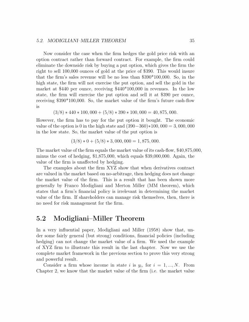
Now consider the case when the firm hedges the gold price risk with anoption contract rather than forward contract. For example, the firm couldeliminate the downside risk by buying a put option, which gives the firm theright to sell 100,000 ounces of gold at the price of $390. This would insurethat the firm’s sales revenue will be no less than $390*100,000. So, in thehigh state, the firm will not exercise the put option, and sell the gold in themarket at $440 per ounce, receiving $440*100,000 in revenues. In the lowstate, the firm will exercise the put option and sell it at $390 per ounce,receiving $390*100,000. So, the market value of the firm’s future cash-flowis
(3/8) ∗ 440 ∗ 100, 000 + (5/8) ∗ 390 ∗ 100, 000 = 40, 875, 000.
However, the firm has to pay for the put option it bought. The economicvalue of the option is 0 in the high state and (390−360)∗100, 000 = 3, 000, 000in the low state. So, the market value of the put option is
(3/8) ∗ 0 + (5/8) ∗ 3, 000, 000 = 1, 875, 000.
The market value of the firm equals the market value of its cash-flow, $40,875,000,minus the cost of hedging, $1,875,000, which equals $39,000,000. Again, thevalue of the firm is unaffected by hedging.
The examples about the firm XYZ show that when derivatives contractare valued in the market based on no-arbitrage, then hedging does not changethe market value of the firm. This is a result that has been shown moregenerally by Franco Modigliani and Merton Miller (MM theorem), whichstates that a firm’s financial policy is irrelevant in determining the marketvalue of the firm. If shareholders can manage risk themselves, then, there isno need for risk management for the firm.
5.2 Modigliani–Miller Theorem
In a very influential paper, Modigliani and Miller (1958) show that, un-der some fairly general (but strong) conditions, financial policies (includinghedging) can not change the market value of a firm. We used the exampleof XYZ firm to illustrate this result in the last chapter. Now we use thecomplete market framework in the previous section to prove this very strongand powerful result.
Consider a firm whose income in state i is yi, for i = 1, ..., N . FromChapter 2, we know that the market value of the firm (i.e. the market value

36 CHAPTER 5. WHY SHOULD FIRMS MANAGE RISK?
of the income plan (y1, ..., yN)) is
V = P (y) =
N∑
i=1
yipi.
If the firm buys a financial security a = (a1, ..., aN ) to change the distri-bution of its income across states, then, the new income profile is given byy = (y1 + a1, ..., yN + aN ), and the firm’s market value is now
V = P (y)− P (a)
where P (a) is the market value of the security a. But
P (y) =
N∑
i=1
[yi + ai]pi,
and
P (a) =N∑
i=1
aipi.
So,
V =
N∑
i=1
[yi + ai]pi −N∑
i=1
aipi =
N∑
i=1
yipi = V.
That is, the value of the firm before and after the firm purchased the financialsecurity are the same—the firm’s financial policy does not affect the firm’smarket value. This irrelevance result is the now celebrated Modigliani–MillerTheorem.
Note that in the proof of the theorem above, we have not put any re-strictions on the income y implied by the firm’s financial policy. In reality,however, firms may have limited liability and, therefore, the firm’s incomeshould always be non-negative: when the implied income is negative, thefirm will simply go bankrupt and pays zero to those who have claims on thefirm. In the following we show that even if there is the possibility of default,Modigliani–Miller Theorem still holds.
Assume that the firm chooses a combination of equity and bond to financeits investment. Let the firm issue a bond which promises to pay the bondholder a fixed amount R. Let VD be the funds that the firms raised throughthe bond issue. Then, the total value to the firm is the value of equity income
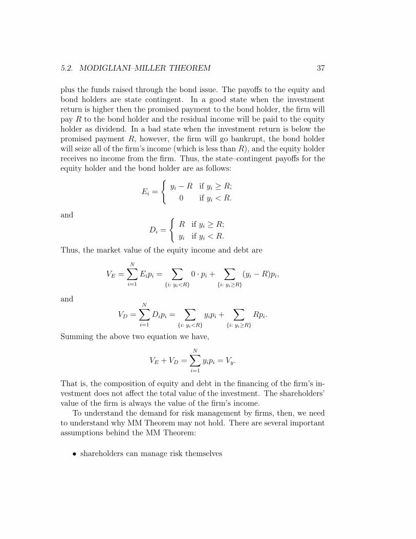
5.2. MODIGLIANI–MILLER THEOREM 37
plus the funds raised through the bond issue. The payoffs to the equity andbond holders are state contingent. In a good state when the investmentreturn is higher then the promised payment to the bond holder, the firm willpay R to the bond holder and the residual income will be paid to the equityholder as dividend. In a bad state when the investment return is below thepromised payment R, however, the firm will go bankrupt, the bond holderwill seize all of the firm’s income (which is less than R), and the equity holderreceives no income from the firm. Thus, the state–contingent payoffs for theequity holder and the bond holder are as follows:
Ei =
{yi − R if yi ≥ R;
0 if yi < R.
and
Di =
{R if yi ≥ R;
yi if yi < R.
Thus, the market value of the equity income and debt are
VE =
N∑
i=1
Eipi =∑
{i: yi<R}0 · pi +
∑
{i: yi≥R}(yi −R)pi,
and
VD =
N∑
i=1
Dipi =∑
{i: yi<R}yipi +
∑
{i: yi≥R}Rpi.
Summing the above two equation we have,
VE + VD =
N∑
i=1
yipi = Vy.
That is, the composition of equity and debt in the financing of the firm’s in-vestment does not affect the total value of the investment. The shareholders’value of the firm is always the value of the firm’s income.
To understand the demand for risk management by firms, then, we needto understand why MM Theorem may not hold. There are several importantassumptions behind the MM Theorem:
• shareholders can manage risk themselves

38 CHAPTER 5. WHY SHOULD FIRMS MANAGE RISK?
• there exist a complete, frictionless financial market;
• investment opportunities is independent of the financial decisions;
• no bankruptcy cost;
• no taxes.
Note that the first assumption is not needed for the MM Theorem per se. Butit is an important reason why shareholders care only about the market value,not the risk of a firm. We now consider in turn each of these assumptionsand discuss why and when these assumptions may not hold and, therefore,there are needs for firms to manage risk.
5.3 Shareholders may not be able to manage
risk effectively themselves.
Risk management usually involves transaction costs. For small shareholders,the transaction costs may be too high relative to the benefits of risk man-agement. Therefore, they may not want to manage risk themselves. Never-theless, they would benefit from risk management since they are risk–averse.By having the firm manage the risk, the transaction costs that would haveincurred independently by many small shareholders are now incurred by thefirm only. Because of the economy of scale, the average transaction cost toeach individual shareholder is much smaller in this case and may justify theuse of risk management by the firm. A crucial condition for this argument tobe valid, however, is that shareholders are similar to each other so that thereare risk management strategies that can benefit most of the shareholders.
Sometimes large shareholders may find it difficult to manage themselveseffectively the firm’s risk. This is especially true for inside shareholders suchas Bill Gates, who is a large shareholder of Microsoft. Like any other indi-viduals, Bill Gates may want to hedge his risk by hedging against negativeshocks to Microsoft that is beyond his control. However, if he actually triesto implement a hedge by trading derivatives on Microsoft’s stocks, say putoptions, market may perceive it as a bad signal about the Microsoft businessand, therefore, its stock value may fall due to the fact that Bill Gates ishedging against potential fall in the Microsoft stocks.

5.4. CONTROLLING UNDERINVESTMENT WITH HEDGING 39
5.4 Controlling Underinvestment with Hedging
Consider the following example: From previous investment, a firm’s incomeis $1000 with probability 1/2 and $200 with probability 1/2. The firm has$500 debt outstanding. After the income of the firm is realized, and beforethe debt is due, the firm is presented with a risk–free investment project:investing $600 yields $800 in return.
If the firm’s income is $1000, then, by taking the project, the firm’s totalincome would be $1,200. After paying back the debt, the equity holderswould have a residual value of $700. If the project is not taken, however, thetotal income would be $1000, and the equity holders would have a residualvalue of $500. So, the equity holder will invest in the project.
If the firm’s income is $200, then, to invest in the project, the firm hasto come up with additional $400. After the investment, the total incomewould be $800, of which $500 will go to the bond holders and the equityholders would have a residual value of $300. Taking into account the $400additional investment, the equity holder incur a net loss of $100. If theinvestment project is not taken, then the firm would go into default, thebond holders receive $200 and the equity holders receive no income. In thiscase, the equity holders do not have incentive to invest in the project evenif it is clearly profitable project. The reason that the equity holders do notwant to invest in the project is that all the additional returns are capturedby the bond holders when the firm is in financial distress.
If the firm has hedged so that the income in both state is $600 (assumingthat there is no hedging cost), then the firm will always take the investmentproject. So, hedging in this case ensures that the profitable project is takenby the firm and, therefore, increases the value of the firm.
5.5 Reducing Tax Liabilities with Hedging
Governments often give tax credits (i.e., investment tax credits for researchand development expenditures) to firms. When a firm’s income is too low,they will not be able to take advantage of such credits. Risk managementcan help firms to fully take advantage of tax credits by stabilizing income.To see why this is the case, consider the following simple example.
Let y be a firm’s income, which is subject to a flat tax rate, τ , 0 < τ < 1.Suppose that the government allows the firm to write off its first d dollars of

40 CHAPTER 5. WHY SHOULD FIRMS MANAGE RISK?
income as tax credits. So, if the firm’s income is greater than d, then its taxliability is τ(y−d); and if the firm’s income is less or equal to d, then it doesnot have to pay any taxes. That is, the tax liability of the firm with incomelevel y is
T = τ max(y − d, 0).
Figure 4 plots the tax liability as a function of the firm’s income, y. Supposethat with equal probabilities (0.5) the firm’s income may be yl or yh, andthat yl < d < yh. Then, the firm’s expected tax liability is
E[T ] =1
2τ(yh − d).
If the firm has hedged so that its income always equals (assuming no hedgingcost for simplicity)
E[y] =1
2yh +
1
2yl,
then the tax liability is certain and equals
Thedging = τ max(E[y]− d, 0)
Because yl < d, we have
E[y]− d =1
2(yh − d) +
1
2(yl − d) <
1
2(yh − d).
So,
Thedging < τ max(1
2(yh − d), 0) =
1
2τ(yh − d).
That is, the tax liability under hedging is less than the expected tax liabilitywithout hedging. (See Figure 4.)
Insert Figure 4 Here

5.6. DEBT AND HEDGING POLICIES 41
5.6 Debt and Hedging Policies
The reason that a firm may experience financial distress often has to do withproblems of repaying the debt the firm had incurred. Why would a firm issuedebt then? According to the MM theorem, debt financing does not increasethe value of the firm, and therefore, there is not reason for the firm to havedebt financing, especially when debt may increase the probability of financialdistress.
One reason firms issue debt is to reduce its tax liabilities, because interestpayments on debt can be deducted from firms’ cash flows. Therefore, inchoosing its debt level, a firm is faced with a trade-off between tax reductionand increases in the probability of financial distress. We now consider asimple model that can be used to study this trade-off. Consider the modelin Section 4.2. We now introduce a flat-rate tax on firm’s cash-flow. The taxliabilities for the firm is:
Ti =
{t(yi − R) if yi ≥ R;
0 if yi < R.
So, the equity holders’ dividend is given by
Ei =
{(1− t)(yi − R) if yi ≥ R;
0 if yi < R.
In addition, we also introduce a cost of default. That is, the value thatthe debt holder receives in the case of default is yi− cyi, where cyi is the costassociated with default. So, the debt holder’s payoff is given by
Di =
{R if yi ≥ R;
(1− c)yi if yi < R.
Thus, the market value of the equity and debt are, respectively,
VE =N∑
i=1
Eipi =∑
{i: yi<R}0 · pi + (1− t)
∑
{i: yi≥R}(yi −R)pi,
and
VD =N∑
i=1
Dipi = (1− c)∑
{i: yi<R}yipi +
∑
{i: yi≥R}Rpi.

42 CHAPTER 5. WHY SHOULD FIRMS MANAGE RISK?
Summing the above two equations we have
V (R) = VE + VD =
N∑
i=1
yipi − c
∑
{i: yi<R}yipi
− t
∑
{i: yi≥R}(yi −R)pi
.
Note that the value of the firm is now a function of the amount of liabilitiesoutstanding, R. That is, with taxes and default cost, leverage has an effecton the value of the firm.
Consider the following example: N = 2. y1 = e − h, and y2 = e + h.Furthermore, assume that p1 = p2 = 1/2. Now we examine the firm’s optimalchoice of debt level, R.
If R ≤ e− h, then, yi ≥ R for both i = 1 and 2. Thus,
V (R) =
2∑
i=1
yipi − t
[2∑
i=1
(yi −R)pi
]= (1− t)e + tR.
In this case, the optimal debt level should be the maximum possible, R =e− h, which implies that
V 1 = e− th.
Next, consider the case when e − h < R ≤ e + h. In this case, y1 < R andy2 ≥ R. So, we have
V (R) =2∑
i=1
yipi − cy1p1 − t(y2 − R)p2
= e− 1
2c(e− h)− 1
2t(e+ h− R).
Again, it is optimal for the firm to choose the maximum possible debt in thiscase, R = e+ h, which implies that
V 2 = e− 1
2c(e− h) = (1− 1
2c)e+
1
2ch.
Finally, if the firm chooses the debt level that is above e + h, then, the firmwill for sure go bankrupt and we have
V 3 = (1− c)
2∑
i=1
yipi = (1− c)e.
5.6. DEBT AND HEDGING POLICIES 43
Apparently, the firm will not choose a debt level that is above e+h, becausethe value of the firm in that case, V 3, is always lower than the value of thefirm when the debt level is at e + h, V 2. Whether the firm will choose thedebt level to be e− h, or e + h, however, depends on the values of c and t.
V 2 − V 1 = th− 1
2c(e− h).
So, the higher the tax rate is, the more likely that the firm will choose a highdebt level to reduce its tax liabilities. On the other hand, the higher the costof default, c, the more likely that the firm will choose a relatively low levelof debt to reduce the expected default cost. The optimal debt level, then, ischosen based on trading off these two factors.
Now let’s see how hedging affect the firm’s value and the firm’s choice ofdebt level. Since p1 = p2 = 1/2, we know that the market value of (e−h, e+h)is the same as the market value of (e, e). Therefore, the firm can choose tohave its after hedge cash-flow to be e in both states. In this case, if the firmchoose the debt level at R to be the same as e. Then, the firm will not godefault and there will be no taxes to be paid. The total value of the firm isin this case,
V = e.
Apparently, with hedging, the firm has eliminated the trade-off between de-fault and tax reduction.

44 CHAPTER 5. WHY SHOULD FIRMS MANAGE RISK?

Chapter 6
Bond Analytics
6.1 Zero-Coupon Bonds and Coupon Bonds
There are two kinds of bonds. One are the bonds that pay the principalplus interest all at once at the maturity. Such bonds are called zero-couponbonds. The total amount that will be paid a at the maturity is called theface value of the bond. For example, consider a one-year zero-coupon bondwhose current value is $96. Suppose the interest on the bond is $4. Thenthe bond will pay $96+ $4 = $100 at the end of one year, and the face valueof the bond is $100. The effective continuous compounding interest rate onthis bond R is determined by the following equation:
96=e−R100
or R = ln(100/96) = 4.08%. Here, R is the interest rate that can be usedto discount the face value of the bond to get the current market price of thebond.
Now, for any time t, let Z(t) denote the zero coupon bond with a facevalue of $1 paid at time t. Let R(t) be the corresponding interest rate forthe zero-coupon bond. Then, we have P (Z(t)) = e−R(t)t.
The second type of bonds are those that pay coupons in regular timeintervals as well as the principal at the maturity. For example, a two yearUS treasury bond with an annual coupon rate of 8% and principal of $100will have four coupon payments of $4 (half of the annual coupon) at sixmonth, one year, one and half year and two year plus the principal paymentof $100 at two year. Such a coupon bond can be thought of a combination
45
46 CHAPTER 6. BOND ANALYTICS
of four zero coupon bonds: a six month zero coupon bond with face value of$4, a one year zero coupon bond with face value of $4, a one and half yearzero coupon bond with face value of $4, and a 2 year zero coupon bond withface value of $104 (principal plus coupon). That is the two year US treasurybond is a portfolio of four zero-coupon bonds:
4Z(0.5) + 4Z(1) + 4Z(1.5) + 104Z(2),
and the value of this bond is
P (4Z(0.5) + 4Z(1) + 4Z(1.5) + 104Z(2))
= 4P (Z(0.5)) + 4P (Z(1)) + 4P (Z(1.5)) + 104P (Z(2))
= e−R(0.5)0.54 + e−R(1)4 + e−R(1.5)1.54 + e−R(2)2104.
Now consider a portfolio of two coupon bonds. One is a one year couponbond with a coupon rate of 6% and principal of $100. The other is a two yearcoupon bond like the one above. We can write the one year coupon bond as
3Z(0.5) + 103Z(1).
So, the portfolio of the two bonds can be written as
3Z(0.5) + 3Z(1) + 4Z(0.5) + 4Z(1) + 4Z(1.5) + 104Z(2)
= 7Z(0.5) + 107Z(1) + 4Z(1.5) + 104Z(2).
Thus, a portfolio of coupon bonds can also be written as a portfolio of zerocoupon bonds. The value of the portfolio is
7Z(0.5) + 107Z(1) + 4Z(1.5) + 104Z(2)
= e−R(0.5)0.57 + e−R(1)107 + e−R(1.5)1.54 + e−R(2)2104.
The examples above show that a portfolio of bonds always consists of afinite number of payments at a finite number of dates. So, we can alwaysexpress the portfolio as a portfolio of zero coupon bonds:
c1Z(t1) + c2Z(t2) + ...+ cnZ(tn). (6.1.1)
In the first example above, we have n = 1, t1 = 1, and c1 = 100. In theexample of the two year treasury bond, we have n = 4, t1 = 0.5, t2 = 1,t3 = 1.5, and t4 = 2; and c1 = c2 = c3 = 4 and c4 = 104. Finally, in the last

6.2. BOND YIELD AND DURATION 47
example, we also have n = 4, n = 4, t1 = 0.5, t2 = 1, t3 = 1.5, and t4 = 2.However, we have c1 = 7, c2 = 107, c3 = 4, and c4 = 104.
The value of the bond portfolio in (6.1.1) can be written as:
B = P (c1Z(t1) + c2Z(t2) + ...+ cnZ(tn))
= e−R(t1)t1c1 + e−R(t2)t2c2 + ...+ e−R(tn)tncn. (6.1.2)
6.2 Bond Yield and Duration
Equation (6.1.2) shows that the value of a bond portfolio is affected by npotentially different interest rates, R(t1),...,R(tn). The reason is that theportfolio has cash-flows that will occur at different dates and therefore eachof these cash-flow will be discounted by an appropriate interest rate. Itwould be convenient, however, if we can use one interest rate to discountall the cash-flows in the portfolio for determining the value of the portfolio.Such an interest rate is call the yield of the bond portfolio and is definedmathematically as the value of y that solves the following equation:
B = e−R(t1)t1c1+e−R(t2)t2c2+ ...+e−R(tn)tncn = e−yt1c1+e−yt2c2+ ...+e−ytncn.(6.2.1)
For a zero-coupon bond Z(t), we have
B = P (Z(t)) = e−R(t)t
and apparently the yield of the bond is simply R(t). For a coupon bondlike that in (6.1.1), however, the yield of the bond does not correspond to aparticular interest rate. Instead, it is some kind of average of all the relevantinterest rates: R(t1) through R(tn). It is clear from (6.2.1) that the value ofthe bond is inversely related to the yield of the bond: As yield increases, thebond value declines and vice versa. One way to measure the impact of theyield on the value of the bond is calculate the derivative of the bond pricewith respect to the yield. From (6.2.1), then, we have
dB
dy= −
(e−yt1c1t1 + e−yt2c2t2 + ...+ e−ytncntn
).
This equation can be rewritten as follows:
dB = −(e−yt1c1t1 + e−yt2c2t2 + ... + e−ytncntn
)dy

48 CHAPTER 6. BOND ANALYTICS
ordB
B= −e−yt1c1t1 + e−yt2c2t2 + ...+ e−ytncntn
Bdy
If we define
D =e−yt1c1t1 + e−yt2c2t2 + ... + e−ytncntn
B, (6.2.2)
then, we havedB
B= −Ddy. (6.2.3)
The left hand of equation (6.2.3) is the return of the bond: change in thevalue of the bond as a percentage of the current value of the bond. Theequation shows that the bond return is inversely related to the change inbond yield. Furthermore, the magnitude of the negative impact of the yieldon the bond is measured by the quantity D, which is called the duration ofthe bond.
Note that the duration of the bond is a weighted average of the cash-flowpayment time:
D =
(e−yt1c1
B
)t1 +
(e−yt2c2
B
)t2 + ...+
(e−ytncn
B
)tn.
If the bond is a zero-coupon bond, then the duration is simply the maturityof the bond. For coupon bonds, however, the duration is generally less thanthe maturity of the bond because coupons are paid before the maturity date.In general, however, the duration increases with the maturity for both zero-coupon and coupon bonds.
6.3 Value at Risk (VaR): An Example
From equation (6.2.3) we can see that the return of a bond is negativelyrelated to the change in bond yield. If the yield goes down, then the bondreturn increases. Furthermore, the magnitude of the return increase is mea-sured by the duration. So, if an investor thinks that the bond yield will godown and she wants to maximize the return of her investment in a bond port-folio, then she should choose a portfolio with a high duration. This can beaccomplished by investing in long-term bonds. There is a downside of suchan investment strategy, however. If the bond yield goes up rather than goesdown, then the bond return will be negative and the higher the duration is,

6.3. VALUE AT RISK (VAR): AN EXAMPLE 49
the large the decline in the return of the bond. So, the strategy of investingin long duration bond portfolio has the potential of generating high positivereturns as well as large negative returns. In other words, investing in a bondportfolio with a long duration is highly risky.
How do we quantify the risk involved in the investment in bonds? Oneapparent way is to calculate the variance of the bond returns. From equation(6.2.3), we have
V ar
(dB
B
)= D2V ar(dy).
So, the higher the variance of yields changes and the higher the duration ofa bond portfolio, the larger the variance of the bond returns.
In recent years, another measure of risk has been widely used. The mea-sure is called Value at Risk, or VaR. Put it simply, VaR is an upper boundon the potential loss such that the probability that a loss will exceed thisupper bound is very small. For a bond portfolio, we know that
dB = −DBdy.
Therefore, over a reasonably short time interval, the change in the portfolio’svalue is approximately
∆B = −DB∆y (6.3.1)
The potential loss of the bond portfolio is measured by −∆B. A 99% VaRof the bond portfolio can be defined as follows:
Pr (potential loss from the portfolio ≤ VaR99%) = 99%.
From (6.3.1), this equivalent to
Pr (−∆B = DB∆y ≤ VaR99%) = 99%,
or
Pr
(∆y ≤ VaR99%
DB
)= 99%. (6.3.2)
So, to find out the VaR of a bond portfolio, we need to know the distributionof yield change, ∆y. In practice, it is usually assumed that ∆y has a normaldistribution with mean zero and variance σ2∆t, where σ2 is the annual vari-ance of yield change and ∆t is the length of the time interval during whichwe are calculating the potential loss. Under this assumption, if we define
x =∆y
σ√∆t

50 CHAPTER 6. BOND ANALYTICS
then x is a standardized normal variable with mean zero and variance one.The equation (6.3.2) can now be rewritten as the following:
Pr
(x =
∆y
σ√∆t
≤ VaR99%
DBσ√∆t
)= 99%.
From the normal distribution table, we know that
Pr
(x =
∆y
σ√∆t
≤ 2.33
)= 99%.
Thus, we have,VaR99%
DBσ√∆t
= 2.33
orVaR99% = 2.33DBσ
√∆t. (6.3.3)

Chapter 7
Pricing Forwards and Swaps
7.1 Forwards
Throughout this chapter, we will repeatedly use the following property ofno-arbitrage:
P0(αxT + βyT ) = αP0(xT ) + βP0(yT ).
Here, P0(wT ) is the time zero market price of a security whose payoff at timeT is wT , which could be a random variable if the security is risky.
Let St be the price of an asset at time t. Consider a forward contract onthe asset which requires the buyer of the contract to buy the asset at timeT with a fixed price K. The payoff of this forward contract for the buyer(who takes a long position in the contract) is then ST −K at time T . Notethat having K dollar at T is equivalent to having K units of the zero-couponbond that pays one dollar at T . Let Zt(T ) be the market price of this zerocoupon bond at time t (t ≤ T ). Then, the payoff of the forward contract canbe written as ST −KZT (T ) (note that ZT (T ) = 1) and therefore the marketvalue of the contract at time zero is
P0(ST −KZT (T )) = P0(ST )−KP0(ZT (T )).
Let r be the risk-free, continuously compounding interest rate. Then,
P0(ZT (T )) = Z0(T ) = e−rT .
So the time zero value of the forward contract is
P0(ST )− e−rTK.
51

52 CHAPTER 7. PRICING FORWARDS AND SWAPS
The forward price of the asset at time zero, F0, is the value of K such thatthe value of the forward contract is zero. That is, F0 is the solution to thefollowing equation
P0(ST − F0ZT (T )) = P0(ST )− e−rTF0 = 0,
which implies that
F0 = erTP0(ST ).
So, to determine the value of a forward contract and to determine the forwardprice of an asset, we need to figure out how to determine P0(ST ). This isdone again by no-arbitrage argument.
(1) ST is the price of a financial asset that pays no income.In this case, ST is simply the payoff from holding the asset until time T .
Since the cost of buying the asset at time zero is S0, no-arbitrage impliesthat
P0(ST ) = S0
and therefore
P0(ST −KZT (T )) = S0 − e−rTK, and F0 = erTS0.
(2) ST is the price of a financial asset that pays a fixed income I at time T .In this case, the payoff of holding the asset until time T is ST + IZT (T )
instead of ST , so we have the following no-arbitrage condition:
P0(ST + IZT (T )) = S0.
But
P0(ST + I) = P0(ST ) + e−rT I.
So, we have
P0(ST ) = S0 − e−rT I, and F0 = erT (S0 − e−rT I) = erTS0 − I.
(3) ST is the price of a financial asset that pays a fixed income I at timeT1 < T .

7.1. FORWARDS 53
Having I at T1 is the same as having IZT1(T1)at T1. So, from (2), we
have
S0 = P0(ST + IZT1(T1))
= P0(ST ) + IP0(ZT1(T1))
= P0(ST ) + e−rT1I.
−e−rT (er(T−T1)I) = S0 − e−rT1I, and
F0 = erT (S0 − e−rT1I) = erTS0 − er(T−T1)I.
Thus,
P0(ST ) = S0 − e−rT1I
and
F0 = erT (S0 − e−rT1I) = erTS0 − er(T−T1)I.
(4) ST is the price of a stock that pays a fixed dividend yield d. That is, thepayoff of owning the asset from 0 to T is ST e
dT .No-arbitrage condition implies that
S0 = P0(ST edT ) = edTP0(ST ).
Thus,
P0(ST ) = e−dTS0, and F0 = erT (e−dTS0) = e(r−d)TS0.
(5) ST is the price of a foreign currency (the exchange rate).In this case, owning one unit of foreign currency at time zero will give
you erfT units of foreign currency at time T , where rf is the risk-free interestrate in the foreign country. In domestic dollar units, the payoff is ST e
rfT .This is equivalent to an asset that pays a fixed continuous dividend yield rf .From (4), then, we have
P0(ST ) = e−rfTS0, and F0 = e(r−rf )TS0.
Note that F0 is the forward price of a foreign currency, or the forward ex-change rate.
(6) ST is the price of a commodity.
54 CHAPTER 7. PRICING FORWARDS AND SWAPS
Holding commodities may be costly. Let U be the (time zero) presentvalue of the storage cost, then, no-arbitrage condition says that
U + S0 = P0(ST ).
Thus,F0 = erT (S0 + U).
If the holder of the commodity have to pay storage cost continuously andthe cost is proportional to the value of the commodity, then, the presentvalue of holding the commodity to time T is S0e
uT , where u is the rate ofstorage cost. In this case, the no-arbitrage condition is
S0euT = P0(ST ),
which implies thatF0 = e(r+u)TS0.
Note that effect of the storage cost u on the forward price is like having anegative dividend −u.
Sometimes people hold commodities for reasons other than hedging orspeculation. For example, a firm may hold inventories of a commodity tomeet unexpected future demand. In this case, holding commodity may ac-tually generate some benefits to the holder. As a result, the actual economiccost of holding a commodity is less than S0e
uT . In this case, a firm is willingto hold the commodity even if P0(ST ) < S0e
uT . This implies that
F0 = erTP0(ST ) < e(r+u)TS0.
That is, since the party who delivers the commodity at T enjoys some benefitsfrom holding the commodity, she is willing to charge a forward price that islower than implied by pure financial arbitrage. We measure the benefits bythe so-called convenience yield y, which is the number such that
F0 = e(r+u)TS0e−yT = e(r+u−y)TS0.
When F0 < e(r+u)TS0, the convenience yield y > 0.
Problem 1: Let Zt(t2) be the time t price of a zero-coupon bond that paysone dollar at time t2. Consider a forward contract that allows one to buy thezero-coupon bond at t1 (t1 < t2). Derive the expression for forward price the

7.2. SWAPS 55
zero-coupon bond, P (t1, t2). Suppose that R(0, t) is the zero-coupon interestrate for the period from 0 to t, (i.e., Z0(t) = e−R(0,t)t), find the forwardinterest rate f(t1, t2) such that
P (t1, t2) = e−f(t1,t2)(t2−t1).
Problem 2: Consider a forward contract on a 5 year coupon bond thatsettles in one year. Suppose that the bond pays a coupon of C dollar semi-annually and that the zero-coupon interest rate is constant, r. Let B0 bethe price of the 5 year coupon bond today. Express the forward price as afunction of r, C and B0.
7.2 Swaps
Consider a standard interest rate swap. Let A and B denote the partythat pays floating interest rates and the party that pays a fixed interestrate, respectively. Let T be the maturity of the swap, and assume thatthe frequency of the payment is m times per year. So the total number ofpayment dates are n = mT , and the time interval between two consecutivepayments are ∆ = 1/m. For example, for a 5 year swap with quarterlypayment frequency we have T = 5, m = 4, n = 20 and ∆ = 0.25.
Let ti = i/m be the iTh payment date of the swap. Then, we haveti−1 = ti −∆. (In the example above, t1 = 0.25, t2 = 0.5, ...,t19 = 4.75 andt20 = 5. Let X be the notional amount of the swap. For any t, let Rt(∆) bethe annualized LIBOR (London Interbank Offered Rate) of maturity ∆ thatis determined in the market at time t. By definition, this interest rate is therate such that the if you borrow 1 dollar in the interbank market at time t,you are supposed to repay 1 + 1
mRt(∆) dollar at t+∆. By no arbitrage, we
have
1 = Pt(1 +1
mRt(∆) at t +∆)
Thus, the time t value of a zero-coupon bond with maturity ∆ is
Zt(t+∆) = Pt($1 at t +∆) =1
(1 + 1mRt(∆))
.
In the standard interest rate swap, the payments of party A and B on dateti are 1
mRti−1
(∆)X and 1mRX, respectively. The value of party B’s payments

56 CHAPTER 7. PRICING FORWARDS AND SWAPS
is easy to determine. It is simply a portfolio of n zero-coupon bonds withmaturity ti i = 1, , , , n and size 1
mRX. So,
VB =
[n∑
i=1
Z0(ti)
]1
mRX.
The determination of the value of party A’s payments, however, is more com-plicated because, except for the first payment, all the future n− 1 paymentsare uncertain at time 0. However, for the ith payment, 1
mRti−1
X we knowthat
Pti−1
(1
mRti−1
(∆)X
)= XPti−1
(1
mRti−1
(∆)
)
= X
[Pti−1
(1
mRti−1
(∆) + 1− 1
)]
= X
[Pti−1
(1
mRti−1
(∆) + 1
)− Zti−1
(ti−1 +∆)
]
= X
[(1
mRti−1
(∆) + 1
)Pti−1
($1 at ti)− Zti−1(ti−1 +∆)
]
= X
[(1
mRti−1
(∆) + 1
)1
(1 + 1mRti−1
(∆))− Zti−1
(ti−1 +∆)
]
= X[1− Zti−1
(ti−1 +∆)].
Thus, the time zero value of the ith payment of party A is
P0
(Pti−1
(1
mRti−1
(∆)X
))
= P0
(X[1− Zti−1
(ti−1 +∆)])
= XP0
($1− Zti−1
(ti−1 +∆) at ti−1
)
= X [Z0(ti−1)− Z0(ti)] .
Note that ti−1 + ∆ = ti. Therefore, the total value of the floating sidepayments is
VA =n∑
i=1
X [Z0(ti−1)− Z0(ti)]
= X [Z0(t0)− Z0(tn)] .

7.2. SWAPS 57
Note that t0 = 0 and tn = T . So, we have
VA = X [1− Z0(T )] .
So, for the party that receives floating rates, the value of the swap is
Pfloat = VA − VB = X [1− Z0(T )]−[
n∑
i=1
Z0(ti)
]1
mRX
or
Pfloat = X −{[
n∑
i=1
Z0(ti)
]1
mRX + Z0(T )X
}
Note that the second term (inside the big bracket) is the value of a couponbond with principal X and annualized coupon rate R.
When the two parties entered into the swap, the value of the paymentson both sides must be the same. So, at the time when the swap is entered,the fixed interest rate R must be such that
VA = X [1− Z0(T )] = VB =
[n∑
i=1
Z0(ti)
]1
mRX,
which implies that
R = m1 − Z0(T )n∑
i=1
Z0(ti).
This fixed rate that makes the swap has zero market value is called the swaprate.
Problem 3. Assume that the (continuous compounding) zero coupon inter-est rates are given by the following table:
1. Calculate the swap rate for 1 year, 2 year and 5 year swaps, respectively.(Assuming semi-annual payment. You can use interpolation to findmissing zero-coupon interest rates.)
2. Consider the five year swap. Suppose that after two months, the zero-coupon yield curve remains the same as in the table above. Calculatethe value of the swap that was entered two months ago for the partywho receives floating interest rates.

58 CHAPTER 7. PRICING FORWARDS AND SWAPS
Maturity annualized zero coupon rate
1 month 0.5%2 month 0.75%3 month 1%6 month 1.25%9 month 1.5%1 year 1.75%2 year 2.5%3 year 3.5%4 year 4.5%5 year 5.5%
7.3 Forward Rates and Swaps
If two parties negotiate on a future loan transaction, what interest rate shouldthey agree on so that there would be no arbitrage? Consider the followingcase: Party A plans to borrow $100 from party B a year from now andwill pay the borrowed amount plus interest back to B 3 month later. Theinterest rate used in the transaction is called the forward rate. Let F be thesimple compounding annualized interest rate, then the transaction involvesthe following cash flows:
• In 1 year, B pays A 100 dollars.
• In 1.25 year, A pays B 100(1 + 0.25F ) dollars.
For there to be no-arbitrage, the current value of those two payments haveto be the same. So, the forward rate f has to satisfy the following condition:
P0(100 in 1 year)= P0(100(1 + 0.25F ) in 1.25 year)
Using the definition of zero-coupon bonds, we have
P0(100 in 1 year)= 100Z0(1)
andP0(100(1 + 0.25F ) in 1.25 year) = 100(1 + 0.25F )Z0(1.25)
Thus, we have100Z0(1) = 100(1 + 0.25F )Z0(1.25)

7.4. FROM SIMPLE COMPOUNDING TO CONTINUOUS COMPOUNDING59
which implies
F =Z0(1)− Z0(1.25)
0.25Z0(1.25)
More generally, using the argument similar to the one above we can showthat the annualized simple compounding forward rate for a loan in time tthat repays back in time t′ is
F (t, t′) =Z0(t)− Z0(t
′)
(t′ − t)Z0(t′)
From the previous section, we know that the value of the ith floatingpayment is
X [Z0(ti−1)− Z0(ti)]
From the forward rate formula above we can rewrite the value of the ithfloating payment of a swap as
Z0(ti)∆F (ti−1, ti)X
That is, the value of receiving the floating rate is the same as receiving thecorresponding forward rate. Therefore, the swap rate is the fixed rate suchthat
n∑
i=1
Z0(ti)∆[F (ti−1, ti)−R
]X = 0
which implies another way of calculating the swap rate:
R =
∑ni=1 Z0(ti)F (ti−1, ti)∑n
i=1 Z0(ti)
In other words, the swap rate is a weighted average of the forward rates.
Problem 4. Using the table in Problem 3 to calculate the the followingforward rates: F (1, 2), F (2, 3), F (3, 4), F (4, 5).
7.4 From Simple Compounding to Continuous
Compounding
The forward rate that we studied in the previous section is a simple com-pounding rate. To find the continuous compounding forward rate, f(t, t′),

60 CHAPTER 7. PRICING FORWARDS AND SWAPS
note the definition is that
e(t′−t)f(t,t′) = 1 + (t′ − t)F (t, t′)
Substituting the formula for simple compounding forward rate into the equa-tion above yields the following:
e(t′−t)f(t,t′) = 1 + (t′ − t)
Z0(t)− Z0(t′)
(t′ − t)Z0(t′)=
Z0(t)
Z0(t′)
Let R(t) be the continuous compounding zero-coupon rate of maturity t, thatis, Z0(t) = e−tR(t), then we have
e(t′−t)f(t,t′) =
e−tR(t)
e−t′R(t′)= et
′R(t′)−tR(t)
which implies the following formula for the continuous compounding forwardrate
f(t, t′) =t′R(t′)− tR(t)
t′ − t.

Chapter 8
Ito Calculus and Black-Scholes
Formula
8.1 Ito Process
Financial variables such as stock prices or interest rates are a function oftime and some random components which make the future changes of thesevariables unpredictable. Ito process is a natural way to capture this propertyof financial variables. We say xt follows an Ito process if the change in xt
over time is given by the following equation:
dxt = a(xt, t)dt+ b(xt, t)dzt (8.1.1)
Here, a(xt, t) and b(xt, t) are two deterministic functions of xt and time t, anddzt is a normally distributed random variable with mean zero and variancedt. We can calculate the expected value and variance of dxt as follows:
E [dxt] = E [a(xt, t)dt+ b(xt, t)dzt] = a(xt, t)dt+ b(xt, t)E[dzt] = a(xt, t)dt
V ar [a(xt, t)dt+ b(xt, t)dzt] = b2(xt, t)V ar [dzt] = b2(xt, t)dt
So, the first and second term of (8.1.1) represent the expected and unexpectedchanges of dxt respectively. For (8.1.1) to represent an Ito process, it is alsorequired that for any t and t′, t 6= t′, dzt and dzt′ are independent. That is,the changes of the random variable zt over any two disjoint time intervals areindependent of each other.
61
62 CHAPTER 8. ITO CALCULUS AND BLACK-SCHOLES FORMULA
Example 1. Let St be the price of a stock at time t. It is usually assumedthat the change in stock price is govern by the following process:
dSt = µStdt+ σStdzt
In this case, a(St, t) = µSt and b(St, t) = σSt. Under this process, the stockreturn over the time interval dt is
dSt
St
= µdt+ σdzt
That is, the expected stock return is µdt and the unexpected stock returnis normally distributed with mean zero and variance σ2dt. Parameter µ iscalled the annualized expected return and σ is called the annual volatility ofthe stock.
Example 2. Let rt be the short rate (the interest rate on a loan that willbe repaid an instant later) at time t. The following is one common way ofdescribing the change of the short rate over time:
drt = β(r − rt)dt+ σdzt
Here β and r are positive constant. So, the expected change in the interestrate is β(r − rt)dt, which is positive if rt is lower than r and negative if rtis greater than r. That is, the interest rate tends to increase when its valueis low and to decline if its value is high. For this reason, we call the processa mean-reverting process. The parameter β determines the speed of meanreversion and r is the long-run mean that the interest rate is reverting to.
8.2 Ito’s Lemma
The price of a derivative security is generally a function of both the time andthe price of the underlying security. For example, the price of an option ona stock is a function of both the stock price and the time to expiration date.If the price of the underlying security follows an Ito process, what about theprice of the derivative security? Ito’s Lemma show that it also follows an Itoprocess.
Ito’s Lemma. Let xt be an Ito process as defined in (8.1.1) and yt is adifferentiable function of xt and t, yt = G(xt, t). Then,
dyt =∂G
∂xt
dxt +∂G
∂tdt+
1
2
∂2G
∂x2t
b2(xt, t)dtt
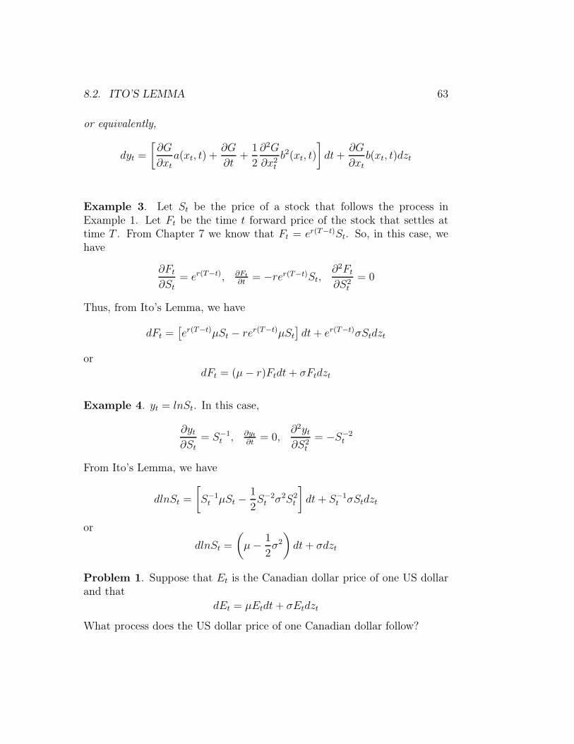
8.2. ITO’S LEMMA 63
or equivalently,
dyt =
[∂G
∂xta(xt, t) +
∂G
∂t+
1
2
∂2G
∂x2t
b2(xt, t)
]dt+
∂G
∂xtb(xt, t)dzt
Example 3. Let St be the price of a stock that follows the process inExample 1. Let Ft be the time t forward price of the stock that settles attime T . From Chapter 7 we know that Ft = er(T−t)St. So, in this case, wehave
∂Ft
∂St= er(T−t), ∂Ft
∂t= −rer(T−t)St,
∂2Ft
∂S2t
= 0
Thus, from Ito’s Lemma, we have
dFt =[er(T−t)µSt − rer(T−t)µSt
]dt+ er(T−t)σStdzt
or
dFt = (µ− r)Ftdt+ σFtdzt
Example 4. yt = lnSt. In this case,
∂yt∂St
= S−1t , ∂yt
∂t= 0,
∂2yt∂S2
t
= −S−2t
From Ito’s Lemma, we have
dlnSt =
[S−1t µSt −
1
2S−2t σ2S2
t
]dt+ S−1
t σStdzt
or
dlnSt =
(µ− 1
2σ2
)dt+ σdzt
Problem 1. Suppose that Et is the Canadian dollar price of one US dollarand that
dEt = µEtdt+ σEtdzt
What process does the US dollar price of one Canadian dollar follow?

64 CHAPTER 8. ITO CALCULUS AND BLACK-SCHOLES FORMULA
8.3 Risk-neutral Pricing
From example 4 in the last section, we know that the infinitesimal changein the log of stock price is normally distributed with mean
(µ− 1
2σ2)dt and
variance σ2dt. Integrating the infinitesimal changes to get the change from0 to T , we have
lnST − lnS0 =
ˆ T
0
(µ− 1
2σ2
)dt+
ˆ T
0
σdzt =
(µ− 1
2σ2
)T + σ (ZT − Z0)
Since ZT − Z0 is normally distributed with mean zero and variance T . Letu = (ZT − Z0) /
√T , then u is normally distributed with mean zero and
variance one. From the equation above, we have,
lnST = lnS0 +
(µ− 1
2σ2
)T + σ
√Tu
orST = S0e
(µ− 1
2σ2)T+σ
√Tu (8.3.1)
That is, the future stock price ST has a log-normal distribution.Consider a derivative contract that has a payoff function h(ST ) at time
T . From Chapter 3 and 4 we know that the value of the derivative contractis the expected payoff discounted by the risk-free interest rate. Here, theexpectation is taken under the risk-neutral probability distribution. That is,
P0 (h(ST )) = e−rT E [h(ST )]
where r is the risk-free interest rate and E means expectation under therisk-neutral distribution. What is the risk-neutral distribution of the stockprice ST ? It can be shown that it is still a log-normal distribution like inequation (8.3.1) but with possibly a different expected return parameter. Fora stock that does not pay dividend, instead of µ, the expected return underthe risk-neutral distribution is the risk-free interest rate r. So, under therisk-neutral distribution, we have
ST = S0e(r− 1
2σ2)T+σ
√Tu (8.3.2)
Thus, the time zero price of an European call option on the stock with strikeprice K is
c0 = e−rT E [max (ST −K, 0)]

8.3. RISK-NEUTRAL PRICING 65
where the expectation is taken under the assumption that ST follows the dis-tribution given in equation (8.3.2). The result is the Black-Scholes formula:
Black-Scholes Formula:
c0 = S0N(d1)− e−rTKN(d2)
Here, N(.) is the cumulative standard normal distribution function and
d1 =ln (S0/K) + (r + 1
2σ2)T
σ√T
d2 =ln (S0/K) + (r − 1
2σ2)T
σ√T
Delta: From the Black-Scholes formula it can easily be shown that
∂c0∂S0
= N(d1)
This partial derivative is called the delta of the call option. It measures thesensitivity of the option price to the change in the price of the underlyingstock. We will show below that calculating delta is important for hedgingoption against stock market risk.
Put-Call Parity and Pricing of Put Options:
Since the payoffs of the call and put options are cT = max(ST − K, 0)and pT = max(K − ST , 0), respectively. We have
cT − pT = ST −K
By no-arbitrage principle,
c0 − p0 = P0(ST −K) = S0 − e−rTK
This is called the put-call parity. From this parity, we can derive the priceand delta of the put option:
p0 = c0 − S0 + e−rTK
∂p0∂S0
= N(d1)− 1

66 CHAPTER 8. ITO CALCULUS AND BLACK-SCHOLES FORMULA
Problem 2. Show that the probability of exercising the call option (Prob [ST > K])is N(d2).Problem 3. Suppose that the stock price is currently $90 and the risk-freeinterest rate is 2%. Calculate the value of an option that pays $1 if the stockprice exceeds $100 one year from now.
8.4 Merton’s No-Arbitrage Argument
Instead of using the risk-neutral pricing method above, the Black-Scholesformula was derived using an no-arbitrage argument suggested by RobertMerton. Let ft = F (St, t) be the price of a derivative security. From Ito’sLemma we have
dF =
[∂F
∂StµSt +
∂F
∂t+
1
2
∂2F
∂S2t
σ2S2t
]dt+
∂F
∂StµStdzt
That is, the unexpected change in the price of the derivative security is alsoa linear function of dzt, the same shock that moves the stock price changeunexpectedly. This suggests that one can form a risk-neutral portfolio byshorting an appropriate amount of the underlying stock. Let δ = ∂f
∂Stand
At = ft − δSt. From the formula above we have
dAt = dft − δdSt =
[∂F
∂t+
1
2
∂2F
∂S2t
σ2S2t
]dt
That is, the change in the value of the portfolio is fully predictable or risk-freeover the infinitesimal time interval dt. By no-arbitrage principle, the returnof the portfolio has to be the same as the risk-free interest rate. So, we have
dAt = rAtdt
or∂F
∂t+
1
2
∂2F
∂S2t
σ2S2t = rF − r
∂F
∂StSt
Rewriting the equation as follows:
∂F
∂t+
∂F
∂St
rSt +1
2
∂2F
∂S2t
σ2S2t = rF
This is a second-order partial differential equation for the unknown functionf . It has exactly the same form as the standard heat equation in physics.

8.4. MERTON’S NO-ARBITRAGE ARGUMENT 67
Whether this equation has an analytical solution depends on the terminalcondition (or payoff at the terminal date) for the function F . For the Eu-ropean call option, the terminal condition is F (ST , T ) = max(ST −K, 0). Ithappens that this terminal condition does yield an analytical solution to theequation and the result is the Black-Scholes formula.
An important insight of the argument presented here is the importanceof delta, the amount of underlying security that one needs to short in orderto hedge the derivative security.

68 CHAPTER 8. ITO CALCULUS AND BLACK-SCHOLES FORMULA
Chapter 9
Value at Risk
In this chapter we discuss the general method of calculation value-at-risk(VaR) that can be applied to bonds, stocks and any derivative securities.
Let Pt be the market value of a portfolio, which may include fixed income,equity, derivatives and other securities. The general rule of thumb is thatthe
VaR99% = 2.37√
Variance(dPt) (9.0.1)
For each problem at hand, the question is how to figure out the variance ofthe change in market value of the portfolio.
Example 1. If Pt is a fixed income portfolio, then
dPt = −DPtdyt
and
Variance(dPt) = Variance(−DPtdyt) = D2P 2t σ
2ydt
where D is the duration of the portfolio, yt the yield, and σy the annualvolatility of the yield change.
Example 2. If Pt is a stock, then,
dPt = µPtdt+ σPtdzt
and
Variance(dPt) = Variance(σPtdzt) = σ2P 2t dt.
69

70 CHAPTER 9. VALUE AT RISK
Example 3. If Pt is a derivative contract on stock. Then Pt = F (St, t) forsome function F . By Ito’s Lemma, we have
dPt =
[∂F (St, t)
∂St
µSt +∂F (St, t)
∂t+
1
2
∂2F (St, t)
∂S2t
σ2S2t
]dt+
∂F (St, t)
∂St
σStdzt
and
Variance(dPt) = Variance
(∂F (St, t)
∂St
σStdzt
)= σ2S2
t
(∂F (St, t)
∂St
)2
dt.
Example 4. If Pt is the market value of a swap contract that pays fixed andreceives floating interest rates with notional principal being 100, then,
Pt = 100− Bt
where Bt is the market value of a bond that pays fixed interest rate and 100is the value of the floating payments plus principal. Thus,
dPt = −dBt
and the variance of dPt is the same as the variance of dBt, which we alreadydiscussed in example 1.

Chapter 10
Credit Risk
Credit risk is about the risk of default. It applies to loans, bonds and swaps.We usually assume that the treasury bonds issued by the US federal gov-ernment has little credit risk and use their prices and yields as benchmarks.For all other borrowers, the interests on their loans or yields on the bondsthey issue are higher than the yields on the treasury bonds of correspondingmaturities. For example, on March 15, 2011, the three month interest rateon a T-bill (US treasury bill) is 0.102%, but the three-month LIBOR, whichis the interest rate charged on three month loans among banks, is 0.309%.So the borrowing cost of a bank is 20 basis points higher than that of theUS government. This difference, called the interest rate spread, is demandedby the lenders to compensate the risk of default that they bear. Similarly,the coupon rate on a five-year treasury bond issued on that day is 2.125%,while the coupon rate on a five-year bond issued by J.P.Morgan (Rated A+)is 3.45%. So the yield spread between the A+ rated firm and the treasury is1.315%, which is again a compensation for the risk of default borne by thebond investors.
The simplest corporate bonds are non-callable bonds. That is, the firmthat issues the bond does not have the option to buy back the bonds fromthe investors at a pre-specified price. There are two types of non-callablecorporate debt: fixed coupon bonds and floating notes. The first type arebonds that pays a fixed coupon rate that is usually quoted as the treasuryplus a spread and the second type pays a floating rate that equals LIBORplus a spread. For example, an eight-year fixed coupon bond issued by anAAA rated firm in 1983 paid treasury plus 60 basis points (0.6%) coupon,and a floating notes of the same maturity issued that year paid LIBOR plus
71

72 CHAPTER 10. CREDIT RISK
25 basis points.In the example above, the yield spread on the fixed-coupon bond is higher
than the yield spread on the floating note. But this is not always the case.Sometimes the spread on a floating note may be higher than the spread ona fixed-coupon bond with the same maturity. In general, if the credit risk isindependent of the interest rate risk, then the spread on floating notes willbe higher (lower) if the forward rate increase (decrease) over time. When for-ward rate increases over time, investor expects more payments in the future,but the risk of default increases with time. So the investors of floating noteshave more exposure to credit risk and therefore demand a higher spread.
In summary, when investors face the risk of default on bonds issued bya firm, they demand a spread over the treasury rate as a compensation forthe risk. The higher the risk of default, the higher the spread would be. So,the yield spread between a corporate bond and a treasury bond of the samematurity contains information on investor’s view of the credit risk they face.In the following we discuss how these information can be used to price acredit derivative instrument called credit default swap.
10.1 Credit Default Swaps
Credit Default Swaps (CDS) is a credit derivative that is used to hedge orspeculate on credit risk (the risk of default). There are CDS on a particularfirm or institution (single name CDS) and CDS on a grouped of firms orinstitutions. Here we will discuss CDS on a particular firm or institutiononly. A CDS is a transaction between two parties. One party buys protectionagainst the default risk by paying selling party a constant premium at regulartime intervals for a pre-specified length of period. During the period, ifdefault occurs, the seller of the CDS will compensate the buyer the fullamount of his loss due to default. So a CDS is a derivative contract basedon a risky bond or risky loan.
Let’s first define some notations:
• P (t1, t2) = forward price of risky zero coupon bond issued at t1 thatpromises to pay $1 at t2. (Think of this as a bond issued by a firm, a

10.1. CREDIT DEFAULT SWAPS 73
government or a financial institution that has potential risk of default.Like in the case of risk-free bonds, one can use the bootstrap methodsto calculate the zero-coupon interest rates of corporate bond by usingthe information on the yield of risky coupon bonds.)
• P ∗(t1, t2) = forward price of a risk-free zero coupon bond issued att1 that will pay $1 at t2. (Think of this as a bond issued by the USTreasury.)
• f(t1, t2) = risky forward rate (i.e. P (t1, t2) = e−f(t1,t2)(t2−t1).)
• f ∗(t1, t2) = risk-free forward rate (i.e. P ∗(t1, t2) = e−f∗(t1,t2)(t2−t1).)
• s(t1, t2) = f(t1, t2) − f ∗(t1, t2) = forward spread between risky andrisk-free forward rates.
• h(t1, t2) = expected proportional loss from the risky bond between t1and t2.
• Q(t1, t2) = survival probability (or probability of no default) betweent1 and t2.
• δ = recovery rate.
Calculating h(t1, t2) from forward spread: The expected proportional lossshould be embedded in the market price of the risky bond. So, we have
P (t1, t2) = P ∗(t1, t2) (1− h(t1, t2))
(Note that here the expectation is taken under the risk-neutral probabilitydistribution.) Thus,
h(t1, t2) = 1− P (t1, t2)
P ∗(t1, t2)= 1− e−s(t1,t2)(t2−t1).
Finding survival probability: Probability of default is 1 − Q(t1, t2). If theissuer does not default, full promised value will be received. If the issuerdefaults, then only proportion δ of the promised value will be recovered. So,the expected value of the risky bond is
P (t1, t2) = Q(t1, t2)P∗(t1, t2) + [1−Q(t1, t2)] δP
∗(t1, t2)
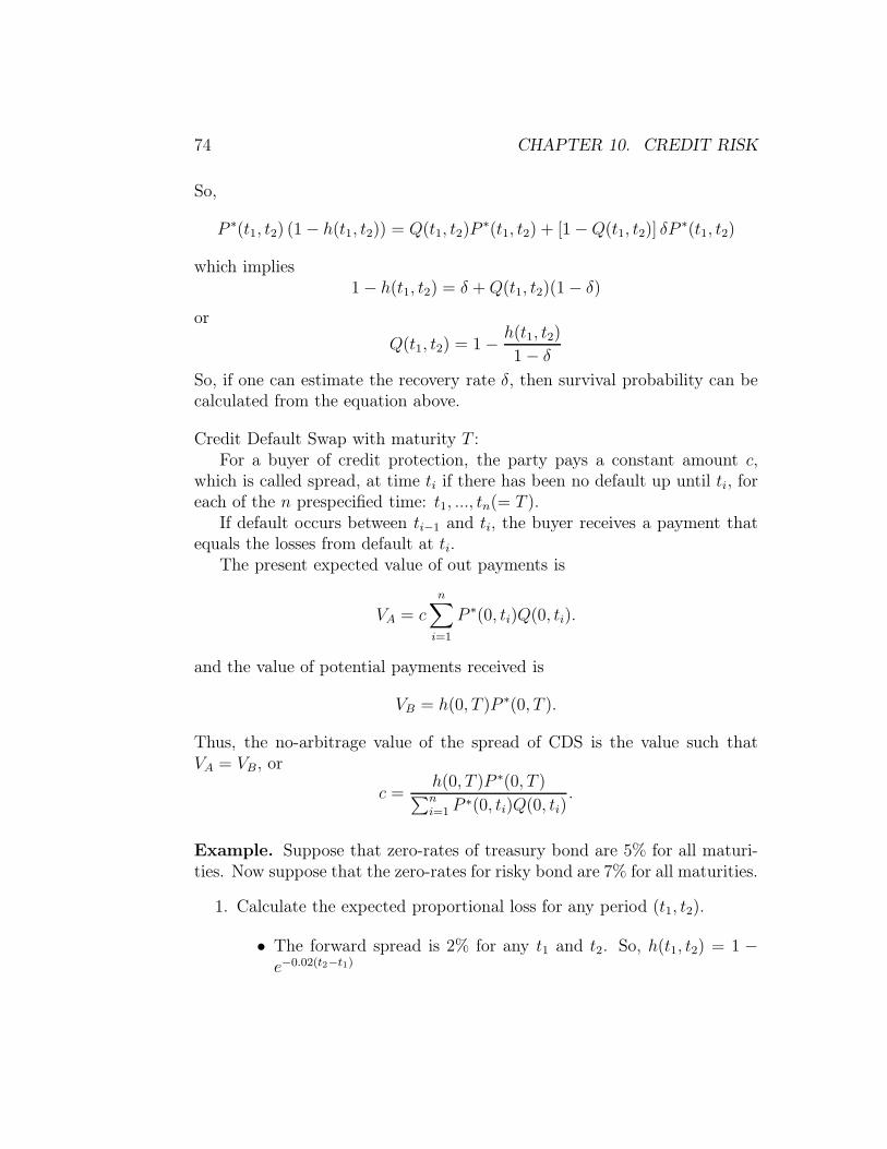
74 CHAPTER 10. CREDIT RISK
So,
P ∗(t1, t2) (1− h(t1, t2)) = Q(t1, t2)P∗(t1, t2) + [1−Q(t1, t2)] δP
∗(t1, t2)
which implies1− h(t1, t2) = δ +Q(t1, t2)(1− δ)
or
Q(t1, t2) = 1− h(t1, t2)
1− δ
So, if one can estimate the recovery rate δ, then survival probability can becalculated from the equation above.
Credit Default Swap with maturity T :For a buyer of credit protection, the party pays a constant amount c,
which is called spread, at time ti if there has been no default up until ti, foreach of the n prespecified time: t1, ..., tn(= T ).
If default occurs between ti−1 and ti, the buyer receives a payment thatequals the losses from default at ti.
The present expected value of out payments is
VA = c
n∑
i=1
P ∗(0, ti)Q(0, ti).
and the value of potential payments received is
VB = h(0, T )P ∗(0, T ).
Thus, the no-arbitrage value of the spread of CDS is the value such thatVA = VB, or
c =h(0, T )P ∗(0, T )∑ni=1 P
∗(0, ti)Q(0, ti).
Example. Suppose that zero-rates of treasury bond are 5% for all maturi-ties. Now suppose that the zero-rates for risky bond are 7% for all maturities.
1. Calculate the expected proportional loss for any period (t1, t2).
• The forward spread is 2% for any t1 and t2. So, h(t1, t2) = 1 −e−0.02(t2−t1)

10.2. USING STOCK MARKET INFORMATION TO ASSESS CREDIT RISK75
2. If the recovery rate is 0.5, what is the survival probability between(t1, t2)?
• Q(t1, t2) = 1− h(t1,t2)1−δ
= 1− 2(1− e−0.02(t2−t1)
)= 2e−0.02(t2−t1) − 1
3. What is the market spread for a CDS? (Assuming annual paymentfrequency.)
c =
[1− e−0.02T
]e−0.05T
∑ni=1 e
−0.05ti [2e−0.02ti − 1]
• See attached excel spreadsheet for calculating the CDS spread fordifferent maturities.
When there is an active market of CDS, the formula for the CDS spreadcan also be used along with yield spread to estimate the recovery rate. Tosee this, we substitute the formula for the survival probability into the CDSspread formula to arrive at the following equation:
c =h(0, T )P ∗(0, T )
∑ni=1 P
∗(0, ti)[1− h(0,ti)
1−δ
]
Since the information on yield spreads will allow us to calculate h(0, ti) forall i, the only unknown in the right hand side of this equation is the recoveryrate δ. If we know what the value of CDS spread c is in the market, thenwe can use this equation to find the implied value of δ that will match thepredicted c with the observed c.
10.2 Using Stock Market Information to Assess
Credit Risk
In the previous section we discussed how to use the information on yieldspreads to assess a company’s credit risk. However, for some companiesthere may not be an active market for the bonds they issued. As a result,we may not have up to date information about the market value of its debt,which is needed to determine yield spreads. In these cases, Robert Merton

76 CHAPTER 10. CREDIT RISK
suggested a method that utilizes a company’s stock price to assess its creditrisk. The method is based on the idea that a firm’s value is the sum of equityand debt and the former is effectively an option on the underlying assets ofthe firm.
Let At be the value of the firm’s underlying asset at time t and F be thevalue of outstanding debt that has to be paid back at some specific time T .Then, the equity and debt values at time T are1
ET = max {AT − F, 0} DT = min {F,AT}
What we want to know is the survival probability evaluated at time t = 0(the probability of default is just one minus the survival probability):
Q = Prob0 [AT ≥ F ]
We assume that the underlying asset follows the following Ito process underthe risk-neutral distribution:
dAt = rAtdzt + σAAtdzt
Here r = r − λ, r is the risk-free interest rate and λ is the cash payout rate(e.g, the dividend/asset ratio). From Problem 2 of Chapter 8 we know that
Q = N(d2)
where N(.) is the standard normal cumulative distribution function and
d2 =ln (A0/F ) + (r − 1
2σ2A)T
σA
√T
However, we may not have good information about the current value of theassets, A0, and its volatility, σA. Fortunately, the Black-Scholes formula foroptions allows us to infer those values from the current price and volatilityof the firm’s equity.
From the Black-Scholes formula, we have
E0 = A0e−λTN(d1)− e−rTFN(d2) (10.2.1)
whered1 = d2 + σA
√T
1For simplicity we assume that there is no tax nor default cost.

10.2. USING STOCK MARKET INFORMATION TO ASSESS CREDIT RISK77
Note that the formula here is slightly different from the formula in Chapter8 because we allow for the asset to have cash payouts. Using Ito’s Lemma,we also have
V ar [dE0] =
(∂E
∂A
)2
σ2AA
20
and we also know that∂E
∂A= e−λTN(d1)
So, the volatility of the equity price is
σE =
√V ar [dE0]
E0=
∂E
∂A
A0
E0σA (10.2.2)
Since we can observe equity price E0 and estimate its volatility σE , equation(10.2.1) and (10.2.2) can be used to jointly solve for the values of A0 and σA.
Problem 1. There are two companies that have the same current value ofassets, the same debt outstanding and the same cash payout rate. If onecompany has higher asset volatility than the other one, what do you thinkwould be the differences in equity price and default probability of the twocompanies?Problem 2. Use Ito’s Lemma to derive equation (10.2.2).

78 CHAPTER 10. CREDIT RISK

Chapter 11
Using Swaps to Hedge Interest
Rate Risk
In this chapter we discuss two examples when interest rate swap can help afirm to hedge its interest rate risk.
Hedging Interest Rate Risk by Mortgage Banks
Mortgage banks take deposits from households and then lend the money outas mortgages to home buyers. Because the deposits are usually short term,the interest rates paid on deposits have to move with the market. Otherwise,depositors will take their money elsewhere. Mortgages, on the other hand,are long-term loans and many of them have a fixed interest rate. Supposethat a mortgage bank received from depositors 100 million dollars and lentthem out as 5 year mortgages at a fixed rate equals the 5-year treasuryrate plus a spread. Suppose that the bank has some reserve money in itssafe so that it can meet the demand for occasional cash withdraws from thedepositors. Also suppose that there will always be new depositors replacingold depositor so that the total value of the pool of deposits stay at 100 milliondollars. Finally, suppose that the average term of the deposits is 3-monthand the average interest rate the bank pays to the depositors is the 3-monthLIBOR.
On March 17, for example, the 5-year treasury yield is 1.909% and the3-month LIBOR is 0.3%. If the bank started this business today, they prob-ably could charge a fixed rate of 3.5% on the five year mortgages. So, if
79

80 CHAPTER 11. USING SWAPS TO HEDGE INTEREST RATE RISK
the LIBOR stays at its current level, the bank will make a profit of (3.5-0.3)%x100million=3.2 million dollars each year. In reality, however, LIBORmay go down or go up in the next five years. If the LIBOR goes above 3.5%within the next five year, however, the bank will start to lose money. Tohedge this risk, the bank may enter into a fix for floating swap. On the swapmarket, the fixed rate on a 5 year swap for a AAA rated bank is 2.35%. Thisbank is rated slightly lower than AAA and therefore it has to pay a higherfixed rate, say 2.85%, on the 5-year swap. As a result of entering the swap,the firm will now make a profit of (3.5-2.85)%x100million=650,000 each yearfor sure, independent of how the LIBOR will fluctuate in the future—if themortgage borrowers will not repay their loans early.
If the LIBOR continues to be low, some borrowers may want to switch toa mortgage with an adjustable rate rather than paying the fixed rate. Let’ssay that 20 million worth of the mortgage is paid off in one year. Then, afterone year, the bank will receive 3.5%x80million=2.8 million dollars each year.But the bank still have to honor the swap and pay 2.85%x100million=2.85million each year. In that case, the bank would lose 50,000 dollars each year.To hedge this pre-payment risk, the bank may choose to include a clause inthe swap contract that gives it the option to reduce the notional amountof the swap by 20 million dollars at any time. This is equivalent to havea standard swap with a notional amount of 80 million dollars and anotherswap with a notional amount of 20 million dollars plus an option to cancelthe swap. The later is called a cancelable swap. The option to cancel theswap is called a swaption. Of course, the bank has to pay a premium forthe option and it will only have the option if the cost of it is less than thepotential loss of 50,000 dollars per year.
Using Swaps to Reduce Financing Cost
Consider the following case. There are two companies, A and B. Both compa-nies can raise funds from the corporate debt market in two alternative ways:issuing a fixed coupon bond that pays a coupon rate equals the treasury rateplus a spread Si
fix or a floating note that pays a coupon rate equals the LI-BOR plus a spread Si
float. Here i = A or B. Suppose that company A has abetter credit rating than company B so that SA
fix > SBfix and SA
float > SBfloat.
Furthermore, suppose that company B prefers to have a fixed interest pay-ment on its debt and company A prefers to have a floating payment on its

81
debt. Company B has two alternative:
1. Issue a fixed coupon bond.
2. Issue a floating note, but then enter into an interest rate swap withcompany A so that it will receive LIBOR and pay a fixed rate thatequals treasury rate plus S.
Let y be the treasury rate. The financing cost for B is y+SBfix and SB
float+y+Sin the second case. It will choose the second financing method if y + SB
fix >
SBfloat + y + S or equivalently
S < SBfix − SB
float (11.0.1)
Company A also has two alternatives:
1. Issue a floating note.
2. Issue a fixed coupon bond, but then enter into an interest rate swapwith company B so that it will receive treasury rate plus S pay LIBOR.
The financing cost for B is LIBOR+SAfloat and y+SA
fix+LIBOR−(y+S) in
the second case. It will choose the second financing method if SAfix−S < SA
float
or equivalentlyS > SA
fix − SAfloat (11.0.2)
For both companies to be willing to enter into the interest rate swap, then,condition (11.0.1) and (11.0.2) both have to hold. This is only possible if
SAfix − SA
float < SBfix − SB
float
In this case, it is usually said that Company B has a comparative advantagein issuing floating notes and company A has a comparative advantage inissuing fixed coupon bonds. Any S between SA
fix − SAfloat and SB
fix − SBfloat
will make the two companies to be willing to do the swap. The gain fromthe swap for A is SA
float −(SAfix − S
)and the gain from the swap for B is(
SBfix − SB
float
)− S. So the total gain is
(SBfix − SB
float
)−(SAfix − SA
float
).
Example. In 1983, B.F. Goodrich was a US tire company that had a BBBrating and Rabobank-Nederland was an AAA rated financial institution inHolland. The market conditions was such that for a $50 million debt, SA
fix =

82 CHAPTER 11. USING SWAPS TO HEDGE INTEREST RATE RISK
0.6%, SAfloat = 0.25%, SB
fix = 2.4% and SBfloat = 0.5%. (The yield curve was
inverted–short term rate was higher than long-term rate–at that time so thatthe spread on floating notes are lower than on fixed coupon bonds.) In thiscase, the total gain is (2.4%-0.5%)-(0.6%-0.25%)=1.55%. That is, by doingthe swap, the two companies would save 1.55%x50 million =775,000 dollarseach year. Such a large “arbitrage” opportunity exists partly because the twocompanies are in two different bond markets (US and Europe) and back thenthe market integration was not as high as today and the interest rate swaps,was just starting to be used by banks to arbitrage the differences betweenthe two markets. Today, it is quite rare that such a large total gain could berealized by using interest rate swaps.

Chapter 12
Using Options to Hedge
Uncertain Price Exposures
If a firm knows exactly its exposure to some market price risk, it can useeither forwards or options to hedge the Market risk. In this chapter wediscuss how options can be used to hedge price risk when the firm’s exposureis uncertain.
12.1 Hedging in the Cases of Known Exposures
We first start with an example when the exposure is known. A gold miningcompany that knows it will have 10,000 ounces of gold to sell in a fixed timein the future, T . So the firm’s revenue at T will be 10, 000ST , where ST
is the gold price at T . To hedge the gold price risk, it can simply take ashort position of a forward contract on 10,000 ounces of gold that settlesat T . Let F be the forward price, the firm’s revenue after hedging will be10, 000ST + 10, 000(F − ST ) = 10, 000F . This will completely eliminate thefirm’s exposure to gold price risk. Alternatively, if the firm does not want togive up the upside gains in the case when gold price increases but still wantsto cover the down side risk of declining gold price, it can buy an Europeanput option for selling 10,000 ounces of gold at T at a pre-specified price K.So the after hedging revenue will be 10, 000ST + 10, 000max {K − ST , 0} =10, 000max(ST , K). (Of course, the firm has to pay a premium upfront tohave the option.)
83

84CHAPTER 12. USING OPTIONS TO HEDGE UNCERTAIN PRICE EXPOSURES
12.2 Hedging in the Cases of Unknown Expo-
sures
In reality, however, the firm’s exposure to price risk may be uncertain. Forexample, the firm may know how much gold it will be able to produce, butdoes not know exactly when they will be available to the market. In thatcase, the firm can still choose to use a short position forward contract tohedge the risk as long as it chooses a settlement date T that is sufficiently farin the future so that it can be sure that the gold will be available by then.Alternatively, the firm can use an American style put option so that it canchoose any time before T to sell the gold at a prespecified price K. In thiscase the firm can sell the gold at the time when it’s available.
Sometimes the firm may not even sure how much gold it will have. Sup-pose that the firm only knows that the amount of gold it will have at T isbetween 9,000 to 11,000 ounces. In that case, the firm’s exposure is some-where between 9, 000ST and 11, 000ST . In this case, the firm can buy a putoption to sell 11,000 ounces of gold at a fixed price K. If the gold price isabove K, then the firm will let the option expire and sell whatever amountof gold it has at the market price. If the gold price is below K, the firm willsell 11,000 ounces of gold at price K for sure: even if the the firm productionresults in less than 11,000 ounces of gold, the firm can buy the rest of thegold from the market and then sell to the other party of the option contractat price K. This is profitable since the market price is below K. So, in thiscase, the firm’s revenue will be
{QST , if ST ≥ K
QK + (11, 000−Q)(K − ST ) if ST < K
With the put option, the firm ensures that its revenue will be greater or equalto QK for any Q between 9, 000 and 11,000.
The option used above to cover the downside risk could be quite expen-sive. To reduce the hedging cost, the firm may also short a forward contracton 9,000 ounces of gold and buy a put option on 2,000 ounces of gold. Inthis case, the cost of hedging will only be 2/9 of the original hedging cost.The firm’s after-hedging revenue will be
{9, 000K + (Q− 9, 000)ST , if ST ≥ K
9, 000K + (Q− 9, 000)K + (11, 000−Q)(K − ST ) if ST < K

12.2. HEDGING IN THE CASES OF UNKNOWN EXPOSURES 85
Note that 9, 000K+(Q−9, 000)K+(11, 000−Q)(K−ST ) = QK+(11, 000−Q)(K − ST ). In this case, the firm also ensures that its revenue is greater orequal to QK.
Problem. Suppose a firm can produce a car in either Canada or US. Thecost in Canada is $20,000 Canadian dollar and the cost in US is $19,000 USdollar. Currently the Canada-US exchange rate is 1. The firm will start toproduce in six month. Whether the firm will produce in the US or Canadiandepends on the exchange rate. Let Et be the Canadian dollar price of one USdollar. Then, the firm will produce in US if and only if 19, 000ET < 20, 000(T = 0.5). So, the firm’s cost is a function of the exchange rate as well:
CT = min {20, 000, 19, 000ET}
If the firm would like to hedge the exchange rate, what derivative contractshould it use?