Lecture notes in quantitative methods for economists ...
158
Lecture notes in quantitative methods for economists: Statistics module Appunti per il corso di Metodi Quantitativi per Economisti, modulo di Statistica Antonio D’Ambrosio Draft 1 Napoli, Ottobre 2020
Transcript of Lecture notes in quantitative methods for economists ...

Lecture notes in quantitative methods for economists:Statistics module
Appunti per il corso di Metodi Quantitativi per Economisti, modulo diStatistica
Antonio D’Ambrosio
Draft 1
Napoli, Ottobre 2020


Preface
Questi appunti raccolgono gli argomenti che vengono trattati al corso diMetodi Quantitativi per Economisti nell’ambito del corso di Laurea Magis-trale in Economia e Commercio dell’Universita degli Studi di Napoli FedericoII.Non si pretende di fornire agli studenti un materiale migliore rispetto ai tantieccellenti manuali presenti in letteratura, molti dei quali sono consigliati perlo studio di questo insegnamento. Si esortano anzi gli studenti a far riferi-mento alle fonti consigliate durante il loro percorso di studio. Il proposito epiuttosto quello di fornire un indice degli argomenti trattati durante il corso,riunirli tutti in un unico corpus e fornire una breve (e non esauriente) guidaalla riproduzione degli esempi riportati attraverso il software R.Questi appunti sono stati volutamente scritti in lingua inglese per una seriedi motivi:
la letteratura sul tema e quasi interamente disponibile in lingua inglese;
gli studenti frequentanti un corso di laurea magistrale devono esserein grado di studiare e approfondire i temi studiati da fonti in linguainglese;
in virtu della crescente internazionalizzazione delle Universita, e semprepiu frequente avere in aula studenti stranieri, magari frequentanti ilprogramma Erasmus.
Gli argomenti trattati riguardano il modello di regressione lineare ed unaintroduzione all’analisi della varianza. Un programma del modulo statis-tico dell’insegnameto di Metodi Quantitativi per Economisti tarato in questomodo dovrebbe preparare gli studenti allo studio di altre discipline quanti-tative in ambito sia economico che statistico, quali ad esempio econometria,modelli lineari generalizzati, data mining, analisi multivariata, categoricaldata analysis, ecc.Si suppone che gli studenti abbiano frequentato sia un corso di Statisticanel quale si siano affrontati i temi principali dell’inferenza statistica ed una
III

introduzione al modello di regressione lineare, sia un corso di Matematicagenerale in cui si siano affrontati problemi di massimizzazione di funzioni euna introduzione all’algebra delle matrici.Questi appunti sono dinamici: potranno cambiare di anno in anno, potrannoincludere nuovi argomenti, potranno escluderne taluni. La loro struttura simodifichera a seconda delle esigenze didattiche del corso di Lurea, ma soprat-tutto seguendo i commenti degli studenti dai quali mi aspetto, se lo vorranno,consigli e critiche costruttive su come modificare e migliorare l’esposizionedegli argomenti proposti.Anche se l’impostazione di questi appunti a prevalentemente teorica, sono ri-portati diversi esempi riproducibili in ambiente R attraverso una operazionedi ”copia-e-incolla” delle funzioni utilizzate. Si precisa pero che lo scopo none quello di imparare ad usare un linguaggio di programmazione: per questovi sono insegnamenti appositi. Laddove non specificato espressamente, i dataset utilizzati, tutti con estensione .rda (l’estensione dei dati di R) sono scar-icabili dal sito http://wpage.unina.it/antdambr/data/MPQE/.Queste pagine contengono sicuramente errori e imprecisioni: saro infinita-mente grato a chi vorra segnalarli.
IV

Contents
Regression model: introduction and assumptions 1
1 Regression model: introduction and assumptions 1
1.1 Regression analysis: introduction, definitions and notations . . 1
1.2 Assumptions of the linear model . . . . . . . . . . . . . . . . . 2
Model parameters estimate 7
2 Model parameters estimate 7
2.1 Parameters estimate: ordinary least squares . . . . . . . . . . 7
2.2 Properties of OLS estimates . . . . . . . . . . . . . . . . . . . 9
2.2.1 Gauss-Markov theorem . . . . . . . . . . . . . . . . . . 9
2.3 Illustrative example, part 1 . . . . . . . . . . . . . . . . . . . . 11
2.3.1 A toy example . . . . . . . . . . . . . . . . . . . . . . . 11
2.4 Sum of squares . . . . . . . . . . . . . . . . . . . . . . . . . . 13
2.4.1 Illustrative example, part 2 . . . . . . . . . . . . . . . 15
Statistical inference 19
3 Statistical inference 19
3.1 A further assumption on the error term . . . . . . . . . . . . . 19
3.1.1 Statistical inference . . . . . . . . . . . . . . . . . . . . 21
3.1.2 Inference for the regression coefficients . . . . . . . . . 22
3.1.3 Inference for the overall model . . . . . . . . . . . . . . 22
3.2 Illustrative example, part 3 . . . . . . . . . . . . . . . . . . . . 23
3.3 Predictions . . . . . . . . . . . . . . . . . . . . . . . . . . . . 25
3.4 Illustrative example, part 4 . . . . . . . . . . . . . . . . . . . . 29
Linear regression: summary example 1 31
V

Contents
4 Linear regression: summary example 1 314.1 The R environment . . . . . . . . . . . . . . . . . . . . . . . . 314.2 Financial accounting data . . . . . . . . . . . . . . . . . . . . 31
4.2.1 Financial accounting data with R . . . . . . . . . . . . 36
Regression diagnostic 43
5 Regression diagnostic 435.1 Hat matrix . . . . . . . . . . . . . . . . . . . . . . . . . . . . 435.2 Residuals . . . . . . . . . . . . . . . . . . . . . . . . . . . . . 455.3 Influence measures . . . . . . . . . . . . . . . . . . . . . . . . 51
5.3.1 Cook’s distance . . . . . . . . . . . . . . . . . . . . . . 525.3.2 The DF family . . . . . . . . . . . . . . . . . . . . . . 535.3.3 Hadi’s influence measure . . . . . . . . . . . . . . . . . 545.3.4 Covariance ratio . . . . . . . . . . . . . . . . . . . . . . 545.3.5 Outliers and influence observations: what to do? . . . . 55
5.4 Diagnostic plots . . . . . . . . . . . . . . . . . . . . . . . . . . 565.5 Multicollinearity . . . . . . . . . . . . . . . . . . . . . . . . . 59
5.5.1 Measures of multicollinearity detection . . . . . . . . . 60
Linear regression: summary example 2 69
6 Linear regression: summary example 2 696.1 Financial accountig data: regression diagnostic . . . . . . . . . 69
6.1.1 Residuals analysis . . . . . . . . . . . . . . . . . . . . . 706.1.2 Influencial points . . . . . . . . . . . . . . . . . . . . . 786.1.3 Collinearity detection . . . . . . . . . . . . . . . . . . . 83
Remedies for assumption Violations and multicollinearity: ashort overview 87
7 Remedies for assumption violations and Multicollinearity 877.1 Introduction . . . . . . . . . . . . . . . . . . . . . . . . . . . . 877.2 Outliers . . . . . . . . . . . . . . . . . . . . . . . . . . . . . . 877.3 Not independent errors and hetersoscedasticity . . . . . . . . . 88
7.3.1 GLS . . . . . . . . . . . . . . . . . . . . . . . . . . . . 887.3.2 WLS . . . . . . . . . . . . . . . . . . . . . . . . . . . . 89
7.4 Collinearity remedies . . . . . . . . . . . . . . . . . . . . . . . 897.4.1 Ridge regression . . . . . . . . . . . . . . . . . . . . . . 89
7.5 Principal Component Regression . . . . . . . . . . . . . . . . . 907.6 Practical examples . . . . . . . . . . . . . . . . . . . . . . . . 90
7.6.1 GLS regression . . . . . . . . . . . . . . . . . . . . . . 91
VI

Contents
7.6.2 WLS regression . . . . . . . . . . . . . . . . . . . . . . 947.6.3 Ridge regression . . . . . . . . . . . . . . . . . . . . . . 97
7.7 Principal Component Regression . . . . . . . . . . . . . . . . . 104
Categorical predictors and Analysis of Variance 107
8 Categorical predictors and ANOVA 1078.1 Categorical predictors . . . . . . . . . . . . . . . . . . . . . . 107
8.1.1 Multiple categories . . . . . . . . . . . . . . . . . . . . 1158.2 Analysis Of Variance . . . . . . . . . . . . . . . . . . . . . . . 115
8.2.1 One way ANOVA . . . . . . . . . . . . . . . . . . . . . 1168.2.2 Multiple comparisons . . . . . . . . . . . . . . . . . . . 1208.2.3 Regression approach . . . . . . . . . . . . . . . . . . . 121
8.3 Two way ANOVA . . . . . . . . . . . . . . . . . . . . . . . . . 1228.3.1 Balanced two way ANOVA: multiple regression approach1288.3.2 ANOVA: considerations . . . . . . . . . . . . . . . . . 130
8.4 Practical examples . . . . . . . . . . . . . . . . . . . . . . . . 1328.4.1 Regression with categorical predictors . . . . . . . . . . 1328.4.2 One way ANOVA . . . . . . . . . . . . . . . . . . . . . 1408.4.3 Two way ANOVA . . . . . . . . . . . . . . . . . . . . . 144
VII


Chapter 1
Regression model: introductionand assumptions
1.1 Regression analysis: introduction, defini-
tions and notations
Regression analysis is used for explaining or modeling the relationship be-tween a single variable Y, called the response variable, or output variable, ordependent variable, and one or more predictor variables, or input variables,or independent variables or explanatory variables, X1, . . . ,Xp.The data matrix is assumed to be derived from a random sample of n obser-vations (xi1, xi2, . . . , xip, yi), i = 1, . . . , n or, equivalently, an n× (p+ 1) datamatrix.When p = 1, the model is called simple regression; when p > 1 the modelis called multiple regression or sometimes multivariate regression. It can bethe case then there are more than one Y: in this case the model is calledmultivariate multiple regression.The response variable must be continuous as well as the explanatory variablescan be continuous, discrete or categorical. It is possible to extend the linearregression model to response categorical variables through the GeneralizedLinear Models (GLM): probably you will study GLM in the future.Let’s define some notations and definitions.
Let n be the sample size;
Let p denote the number of predictors;
Let Y = (Y1, Y2, . . . , Yn)T be the vector of the dependent variables.
Regression model: introduction and assumptions
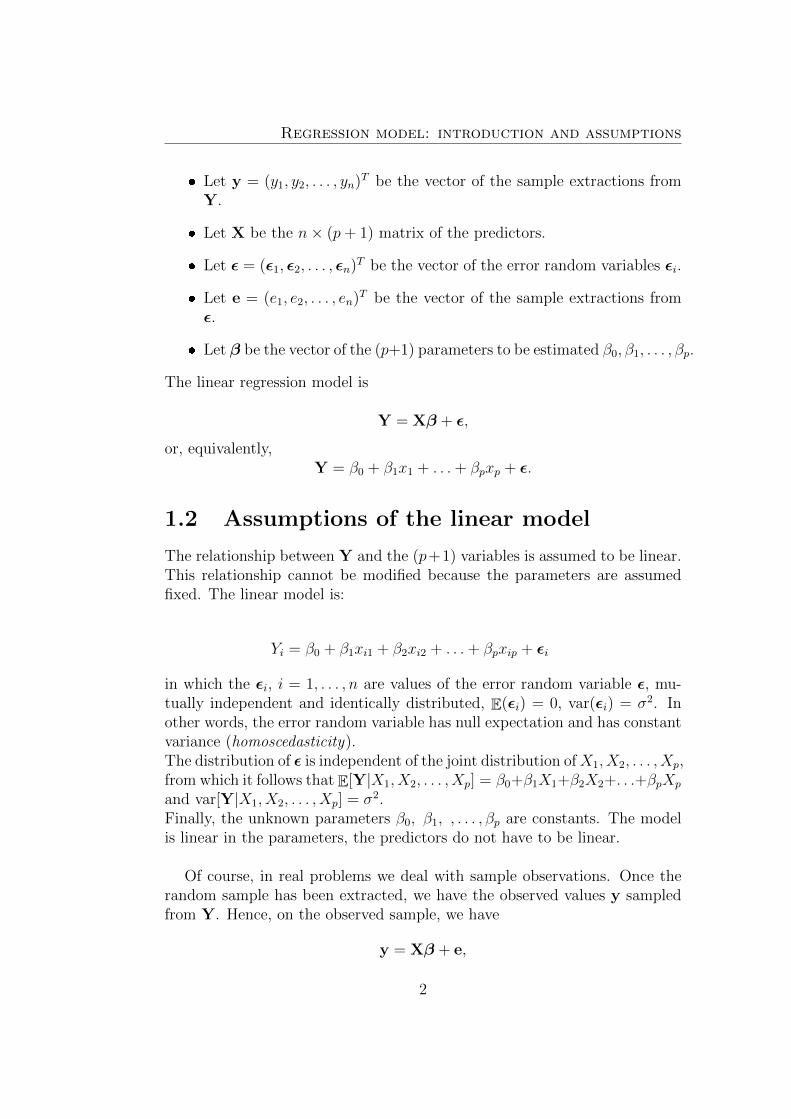
Let y = (y1, y2, . . . , yn)T be the vector of the sample extractions fromY.
Let X be the n× (p+ 1) matrix of the predictors.
Let ε = (ε1, ε2, . . . , εn)T be the vector of the error random variables εi.
Let e = (e1, e2, . . . , en)T be the vector of the sample extractions fromε.
Let β be the vector of the (p+1) parameters to be estimated β0, β1, . . . , βp.
The linear regression model is
Y = Xβ + ε,
or, equivalently,Y = β0 + β1x1 + . . .+ βpxp + ε.
1.2 Assumptions of the linear model
The relationship between Y and the (p+1) variables is assumed to be linear.This relationship cannot be modified because the parameters are assumedfixed. The linear model is:
Yi = β0 + β1xi1 + β2xi2 + . . .+ βpxip + εi
in which the εi, i = 1, . . . , n are values of the error random variable ε, mu-tually independent and identically distributed, E(εi) = 0, var(εi) = σ2. Inother words, the error random variable has null expectation and has constantvariance (homoscedasticity).The distribution of ε is independent of the joint distribution ofX1, X2, . . . , Xp,from which it follows that E[Y|X1, X2, . . . , Xp] = β0+β1X1+β2X2+. . .+βpXp
and var[Y|X1, X2, . . . , Xp] = σ2.Finally, the unknown parameters β0, β1, , . . . , βp are constants. The modelis linear in the parameters, the predictors do not have to be linear.
Of course, in real problems we deal with sample observations. Once therandom sample has been extracted, we have the observed values y sampledfrom Y. Hence, on the observed sample, we have
y = Xβ + e,
2

1.2. Assumptions of the linear model
in which the vector e contains the sample extractions from ε. Note that if weknow the β parameters, than e is perfectly identifiable because e = y−Xβ.
The regression equation in matrix notation is written as:
y = Xβ + e (1.1)
yn×1 =
y1y2...yn
Xn×(p+1) =
1 x11 . . . x1,p1 x21 . . . x2,p...
......
...1 xn1 . . . xn,p
β(p+1)×1 =
β0β1...βp
en×1 =
e1e2...en
The X matrix incorporates a column of ones to include the intercept term(now it should be clear the meaning of the notation in which the predictorsare said to be p + 1: p predictors + the intercept). Let’s see the (classical)assumption of the regression model.
Assumption 1: linearity
Linear regression requires the relationship between the independent and de-pendent variables to be linear. It means that this assumption imposes that
Y = Xβ + ε
.
Assumption 2: the expectation of the random error term is equalto zero
E[ε] =
E[ε1]...
E[εn]
=
0...0
.This assumption implies that E[Y] = Xβ because
E[Y] = E[Xβ + ε] = E[Xβ] + E[ε] = Xβ.
The average values of the random variables that generate the observed valuesof the dependent variable y lie along the regression hyperplane.
3

Regression model: introduction and assumptions
Figure 1.1: Regression hyperplane. the response variable (Album sales) isrepresented on the vertical axis. On the horizonal axes are represented thetwo predictors: Advertising budget and Airplay. The dots are the observedvalues. The regression hyperplane is highlighted in gray with blue countour
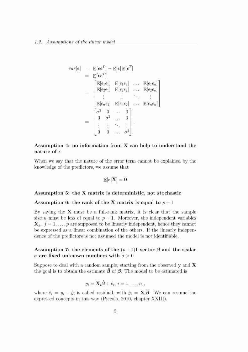
Assumption 3: Homoscedasticity and incorrelation between ran-dom terms
The variance of each error term is constant and it is equal to σ2, furthermorecov(εi, εj) = 0 ∀i 6= j.
var[ε] = E[εεT ] = σ2I, namely
4
1.2. Assumptions of the linear model
var[ε] = E[εεT ]− E[ε]E[εT ]
= E[εεT ]
=
E[ε1ε1] E[ε1ε2] . . . E[ε1εn]
E[ε2ε1] E[ε2ε2] . . . E[ε2εn]...
.... . .
...
E[εnε1] E[εnε2] . . . E[εnεn]
=
σ2 0 . . . 00 σ2 . . . 0...
.... . .
...0 0 . . . σ2
.
Assumption 4: no information from X can help to understand thenature of ε
When we say that the nature of the error term cannot be explained by theknowledge of the predictors, we assume that
E[ε|X] = 0
Assumption 5: the X matrix is deterministic, not stochastic
Assumption 6: the rank of the X matrix is equal to p+ 1
By saying the X must be a full-rank matrix, it is clear that the samplesize n must be less of equal to p + 1. Moreover, the independent variablesXj, j = 1, . . . , p are supposed to be linearly independent, hence they cannotbe expressed as a linear combination of the others. If the linearly indepen-dence of the predictors is not assumed the model is not identifiable.
Assumption 7: the elements of the (p+ 1)1 vector β and the scalarσ are fixed unknown numbers with σ > 0
Suppose to deal with a random sample, starting from the observed y and Xthe goal is to obtain the estimate β of β. The model to be estimated is
yi = Xiβ + ei, i = 1, . . . , n ,
where ei = yi − yi is called residual, with yi = Xiβ. We can resume theexpressed concepts in this way (Piccolo, 2010, chapter XXIII).
5

Regression model: introduction and assumptions
Y = Xβ + ε ⇒ ε = Y −Xβ Teoretical model
y = Xβ + e ⇒ e = y −Xβ General model
y = Xβ ⇒ e = y −Xβ Estimated model
Remember: the vector ε contains the error random variables εi; the vector e,given any arbitrary vector β, contains the realizations of the random variablesεi; the vector e contains the residuals of the model after the estimate of β,that is denoted with β.
6

Chapter 2
Model parameters estimate
2.1 Parameters estimate: ordinary least squares
Let y = Xβ + e be the model. The parameter to be estimated is the vectorof the regression coefficients
β = β0, β1, . . . , βp.
Least squares procedure determines the β vector in such a way that the sumof squared errors are minimized:
n∑i=1
e2i =n∑i=1
(yi − β0 − β1x1i − · · · − βpxpi)
=n∑i=1
(yi −Xiβ)2
= eTe
= (y −Xβ)T (y −Xβ)
We look for β for which f(β) = (y −Xβ)T (y −Xβ) = min. Let’s expandthis product:
f(β) = yTy − βTXTy − yTXβ + βTXTXβ
= yTy − 2βTXTy + βTXTXβ
The function β has scalar values, being β a column vector of length p + 1.The terms βTXTy and yTXβ are equal (two equal scalars), then they can

Model parameters estimate
be summarized with 2βTXTy. The term βTXTXβ is a quadratic form inthe elements of β. Differentiating with respect to f(β) we have
δf(β)
δβ= −2XTy + 2XTXβ,
and setting to zero
−2XTy + 2XTXβ = 0,
we obtain as a solution a vector β such that we obtain the so-called normalequations :
XTXβ = XTy.
Let’s give a look to the normal equations. We have
XTX =
n
∑ni=1 xi1
∑ni=1 xi2 · · ·
∑ni=1 xip∑n
i=1 xi1∑n
i=1 x2i1
∑ni=1 xi1xi2 · · ·
∑ni=1 xi1xip∑n
i=1 xi2∑n
i=1 xi1xi2∑n
i=1 x2i2 · · ·
∑ni=1 xi2xip
......
......
...∑ni=1 xip
∑ni=1 xi1xip
∑ni=1 xi2xip · · ·
∑ni=1 x
2ip
.
As it can be seen, XTX is a (p + 1)× (p + 1) symmetric matrix, sometimescalled sum of squares and cross-product matrix. The diagonal elements con-tain the sum of squares of the elements in each column of X. The off-diagonalelements contain the cross products between the columns of X.The vector XTy is formed by these elements:
XTy =
∑ni=1 yi∑n
i=1 xi1yi∑ni=1 xi2yi
...∑ni=1 xipyi
.
The jth element of XTy contains the product of the vectors xj and y, hencethe vector XTy is a vector of length p + 1 containing the p + 1 productsbetween the matrix X and the vector y.
Provided that the XTX matrix is invertible, the least squares estimate of βis
8

2.2. Properties of OLS estimates
β = (XTX)−1XTy.
Of course, the solution β depends on the observed values y, which are ran-domly drawn samples from the random variable Y. Suppose to extract allthe possible samples of size n from Y: as the random sample varies, theestimates β vary too, being extractions of the Least Squares Estimator B:
B = (XTX)−1XTY.
2.2 Properties of OLS estimates
If the assumptions of the linear regression models are verified, the OLS (Or-dinary Least Squares) estimator is said to be a BLUE estimator (Best LinearUnbiased Estimator). In other words, within the class of all the unbiased lin-ear estimators, the OLS returns the estimator with minimum variance (best).This statement is formally proved with the Gauss-Markov theorem.
2.2.1 Gauss-Markov theorem
The estimator is linear.The estimator B can be expressed in a different way:
B = (XTX)−1XTY
= (XTX)−1XT (Xβ + ε)
= (XTX)−1XTXβ + (XTX)−1XTε
= β + (XTX)−1XTε
= β + Aε
= AY,
where A = (XTX)−1XT and AAT = (XTX)−1. The estimator is linearbecause B = AY, then it is linear combinations of the random variableY.
The estimator is unbiased.The assumption 1 (linearity) implies that B can be expressed as β+Aε(see the point above). Then from assumptions 2 (Average of errorsequal to zero), 4 (deterministic X) and 6 (Constant parameters) itfollows that
E(B) = β + (XTX)−1XT E(ε) = β
9

Model parameters estimate
The estimator is the best within the class of linear and unbiased esti-mators.The first thing to do is determine the variance of B. From assumption3 (Homoscedasticity) we know that E(εεT ) = σ2I. Hence (by recallingthat we can express B = β + (XTX)−1XTε)
var(B) = E[(β − β)(β − β)T ]
= E[((XTX)−1XTε)((XTX)−1XTε)T ]
= E[(XTX)−1XTεεTX(XTX)−1]
= (XTX)−1XT E[εεT ]X(XTX)−1
= (XTX)−1XT (σ2I)X(XTX)−1
= (σ2I)(XTX)−1XTX(XTX)−1
= σ2(XTX)−1
Result 1: var(B) = σ2(XTX)−1.
Suppose that Bo is another linear unbiased estimator for β. As it is alinear estimator, we call C a generic ((p+1)×n) matrix that substitutesA = (XTX)−1XT . We define Bo = CY.It is assumed that the estimator Bo must be unbiased. By recallingthat (first assumption) Y = Xβ + ε, it must be that
E[Bo] = E[CY] = E[CXβ + Cε] = β,
which is true if and only if CX = I.Let’s introduce the matrix D = C − (XTX)−1XT . It allows first toexpress C = D + (XTX)−1XT , and then to see thatDY = CY − (XTX)−1XTY = βo − β. It immediately follows that
10

2.3. Illustrative example, part 1
var(Bo) = σ2[(D + (XTX)−1XT )(D + (XTX)−1XT )T
]= σ2[DDT + DX(XTX)−1 +
+ (XTX)−1XTDT +
+ (XTX)−1XTX(XTX)−1]
= σ2[(XTX)−1 + DDT
]= var(B) + σ2(DDT )
Result 2: var(Bo) = var(B) + σ2(DDT ).
By combining the previous results 1 and 2, it can be seen that
var(Bo)− var(B) = σ2(DDT ),
which is positive semidefinite matrix (i.e., it has non-negative values onthe main diagonal).It is clear that σ2(DDT ) = 0 if and only if D = 0. It happens onlywhen C = (XTX)−1XT producing Bo ≡ B.The conclusion is that, under the assumptions of the linear regressionmodel, the OLS estimator B gives the minimal variance in the class ofunbiased and linear estimators. In a few words, the OLS estimator isa BLUE estimator.
2.3 Illustrative example, part 1
2.3.1 A toy example
Computations by hand
As illustrative example, consider first a toy example in which the computa-tions can be made (if you want) by hand. Suppose to have the following data:
11

Model parameters estimate
y =
64.0561.6468.4375.8586.7751.0377.3852.2751.1284.13
; X =
16.11 714.72 316.02 415.05 416.58 415.22 813.95 314.71 915.48 913.78 3
.
We have n = 10, p = 2. The first to do is add a column of one to the Xmatrix, obtaining
X =
1 16.11 71 14.72 31 16.02 41 15.05 41 16.58 41 15.22 81 13.95 31 14.71 91 15.48 91 13.78 3
.
Let’s compute the XTX matrix:
XTX =
10.00 151.62 54.00151.62 2306.31 824.1754.00 824.17 350.00
.By calling the columns of X const, X1 and X2 respectively, we can see thaton the diagonal we have exactly
∑10i=1 const
2i = n = 10,
∑10i=1X
2i1 = 2306.31
and∑10
i=1X22i = 350.00.
On the off-diagonal elements we have the cross-products∑10
i=1 constiX1i =151.62,
∑10i=1 constiX2i = 54.00 and
∑10i=1X1iX2i = 824.17 (check by your-
self).The determinant of XTX is equal to 4086.68, the cofactor matrix is
(XTX)c =
127946.15 −8560.97 418.94−8560.97 584.00 −54.36
418.94 −54.36 75.04
, yielding to
12

2.4. Sum of squares
(XTX)−1 =
31.31 −2.09 0.10−2.09 0.14 −0.01
0.10 −0.01 0.02
.Now we have to compute the (3× 1) vector XTy:
XTy =
672.6710191.133380.77
.The regression coefficients are computed in this way:
β =
31.31 −2.09 0.10−2.09 0.14 −0.01
0.10 −0.01 0.02
× 672.67
10191.133380.77
=
57.762.24−4.52
In summary, we have β0 = 57.76, β1 = 2.24 and β2 = −4.52.
2.4 Sum of squares
The results obtained with the least squares allow to separate the vector ofobservations y in two parts, the fitted values y = Xβ and the residuals e:
y = Xβ + e = y + e
Since β = (XTX)−1XTy, it follows that:
y = Xβ
= X(XTX)−1XTy
= Hy
The matrix H = X(XTX)−1XT is symmetric (H = HT ), idempotent (H ×H = H2 = H) and is called hat matrix, since it ”puts the hat on the y”,namely provides the vector of the fitted values in the regression of y on X.The residuals from the fitted models are
e = y − y = y −Xβ = (I−H)y.
13

Model parameters estimate
The sum of squared residuals can be written as
eT e =n∑i=1
(yi − yi)2 = (y − y)T (y − y)
= (y −Xβ)T (y −Xβ)
= (yTy − yTXβ − βTXTy + βTXTXβ)
= (yTy − βTXTy)
= yT (I−H)y
This quantity is called the error or (residual) sum of squares and is denotedby SSE.
The total sum of squares is equal to
n∑i=1
(yi − y)2 = yTy − ny2
The total sum of squares, denoted by SST, it indicates the total variation iny that is to be explained by X.
The regression sum of squares is defined as
n∑i=1
(yi − y)2 = βTXTy − ny2 = yTHy − ny2.
It is denoted by SSR.
The ratio of SSR to SST represents the proportion of the total variation iny explained by the regression model. The quantity
R2 =SSR
SST= 1− SSE
SST
is called coefficient of multiple determination. It is sensitive to the magni-tudes of n and p especially in small samples. In the extreme case if n = (p+1)the model will fit the data exactly. In any case, R2 is a measure that doesnot decrease when the number of predictors p increases.In order to give a better measure of goodness of fit, a penalty function canbe employed to reflect the number of explanatory variables used. Using thispenalty function the adjusted R2 is given by
R′2 = 1−
(n− 1
n− p− 1
)(1−R2) = 1− SSE/(n− p− 1)
SST/(n− 1).
14

2.4. Sum of squares
The adjusted R2 changes the ratio SSE/SST to the ratio of SSE/(n−p−1)(an unbiased estimator of σ2
ε , as it will be clear later), and SST/(n− 1) (anunbiased estimator of σ2
Y , as it should be already known).
2.4.1 Illustrative example, part 2
Let’s compute the sum of squares of the model built for the toy example.Remember that the estimated regression coefficients were β0 = 57.76, β1 =2.24 and β2 = −4.52. We then obtain
y = Xβ =
1 16.11 71 14.72 31 16.02 41 15.05 41 16.58 41 15.22 81 13.95 31 14.71 91 15.48 91 13.78 3
×
57.762.24−4.52
=
62.1577.1275.5173.3376.7555.6575.4150.0051.7275.03
.
The residuals are
e = y − y =
64.0561.6468.4375.8586.7751.0377.3852.2751.1284.13
−
62.1577.1275.5173.3376.7555.6575.4150.0051.7275.03
=
1.89−15.49−7.08
2.5210.02−4.62
1.972.27−0.60
9.10
We are ready to compute the sum of squares. We have
SSE =10∑i=1
e2i
= eT e
= 513.80
15

Model parameters estimate
In matrix form:
SSE = eT e
=[
1.89 −15.49 −7.08 2.52 10.02 −4.62 1.97 2.27 −0.60 9.10]×
1.89−15.49−7.08
2.5210.02−4.62
1.972.27−0.60
9.10
= 513.80
The mean value of y is y = 67.27. The total sum of square is then
SST =10∑i=1
(yi − y)2
= yTy − ny2
= 1633.14
In matrix form:
SST = yTy − ny2
=[
64.05 61.64 68.43 75.85 86.77 51.03 77.38 52.27 51.12 84.13]×
64.0561.6468.4375.8586.7751.0377.3852.2751.1284.13
− 10× 67.272
= 1633.14
SSR is then equal to SST − SSE = 1633.14− 513.80 = 1119.34. Indeed wehave
∑10i=1(yi − y)2 = 1119.34.
We are ready to compute the coefficients of multiple determination:
16

2.4. Sum of squares
R2 =SSR
SST=
1119.34
1633.14= 0.69,
R′2 = 1− SSE/(n− p− 1)
SST/(n− 1)= 1− 513.80/(ntoy − ptoy − 1)
1633.14/(ntoy − 1)= 0.60.
17


Chapter 3
Statistical inference
3.1 A further assumption on the error term
We can add a further assumption to the classical assumptions of the lin-ear regression model: the errors are independent and identically normallydistributed with mean 0 and variance σ2:
ε ∼ N (0, σ2I).
.
Since Y = Xβ+ ε, and given assumptions 5 (X has full rank) and 7 (vectorβ and scalar σ are unknown but fixed), it follows that:
var(Y) = var(Xβ + ε) = var(ε) = σ2I,
meaning that
Y ∼ N (Xβ, σ2I).
The assumption of normality of the error term has the consequence thatthe parameters can be estimate with the maximum likelihood method. Theassumption that the covariance matrix of ε is diagonal implies that the entriesof ε are mutually independent (as already known). Moreover, they all havea normal distribution with mean 0 and variance σ2.The conditional probability density function of the dependent variable is
f(yi|X) = (2πσ2)−(1/2)exp
(−1
2
(yi − xiβ)2
σ2
),
the likelihood function is

Statistical inference
L(β, σ2|y,X) =n∏i=1
(2πσ2)−(i/2)exp
(−1
2
(yi − xiβ)2
σ2
)
= (2πσ2)−(n/2)exp
(− 1
2σ2
n∑i=1
(yi − xiβ)2
).
The log-likelihood function is
log(L) = ln(L(β, σ2|y,X))
= −n2ln(2π)− n
2ln(σ2)− 1
2σ2
n∑i=1
(yi − xiβ)2
Remember that∑n
i=1(yi − xiβ)2 = (y − Xβ)T (y − Xβ), namely the sumof the squared errors. The maximum likelihood estimator for the regressioncoefficients is
β = (XTX)−1XTy.
Moreover, the maximum likelihood estimator of the variance is
σ2 =1
n
n∑i=1
(yi − xiβ)2 =1
neT e.
For the regression coefficients, the (mathematical) results are the same: theOLS estimators and the ML estimators have the same formulation. For thevariance of the error terms, the ML estimate returns the unadjusted samplevariance of the residuals e.Why it is important the distributional assumption? It is necessary to as-sume a distributional form for the errors ε to make confidence intervals orperform hypothesis tests. Moreover, ML estimators are BAN estimators:Best Asymptotically Normal.Assuming that ε ∼ N (0, σ2I), since y = Xβ + e we have that
y ∼ N(Xβ, σ2I
).
Then, as linear combinations of normally distributed values are also normal,we find that
B ∼ N(β, σ2(XTX)−1
),
namely
βj ∼ N(βj, σ
2(XTX)−1(jj)
),
20

3.1. A further assumption on the error term
where with (XTX)−1(jj) we indicate the element at the intersection of the j-th
row and the j-th column of the matrix (XTX)−1 (the jth predictor).In a few words, if the errors are normally distributed, then also Y and B arenormally distributed.
3.1.1 Statistical inference
As in practical situations the variance is of course unknown, we need toestimate it. After some computations, one can show that
E
(n∑i=1
e2i
)= E
(eT e)
= σ2(n− p− 1).
In order to show this result, remember that we defined the hat matrix as H =X(XTX)−1XT . Let’s define now the matrix M = I −H. The matrix M has thefollowing properties:
M = MT = MM = MTM.
Moreover, M has rank equal to n − p − 1, as well as tr(M) = n − p − 1. We canwrite the vector of the random variable residuals E = Y −XB as
E = Y −XB = Y −X(XTX)−1XTY = (I−H)Y = MY.
We are able to express the r.v. residuals through the r.v. error:
E = MY = M(Xβ + ε) = MXβ + Mε = Mε.
Hence,
E[ET E] = E[(Mε)T (Mε)]
= E[(εTMTMε)]
= E[tr(εTMTMε)]
= σ2tr(MTM)
= σ2tr(M)
= σ2(n− p− 1).
21

Statistical inference
The conclusion is that
s2 =eT e
n− p− 1=
∑ni=1 e
2i
n− p− 1
is an unbiased estimator of σ2 because
E[S2] =σ2(n− p− 1)
n− p− 1= σ2.
The model has n− p− 1 degrees of freedom. The square root of s2 is namedstandard error of regression and can be interpreted as the average squareddeviation of the dependent variable values y around the regression hyperplan.
3.1.2 Inference for the regression coefficients
Inferences can be made for the individual regression coefficient βj to test thenull hypothesis H0 : βj = β∗j using the statistic
t =(βj − β∗j )√s2(XTX)−1(jj)
,
which, if the null hypothesis is true, has a t distribution with n−p−1 degreesof freedom. Usually, β∗j = 0.A 100(1−a)% confidence interval for βj can be obtained from the expression
βj ± tα/2,(n−p−1)√s2(XtX)−1(jj).
Keep in mind that the inferences are conditional on the other explanatoryvariables being included in the model. The addition of an explanatory vari-able to the model usually causes the regression coefficients to change.
We will denote ESβj as√s2(XtX)−1(jj).
3.1.3 Inference for the overall model
The overall goodness of fit of the model can be evaluated using the F -test(or ANOVA test on the regression). Under the null hypothesis
H0 : β1 = β2 = . . . = βp = 0,
the statistic
22

3.2. Illustrative example, part 3
F =(SSR/p)
(SSE/(n− p− 1))=MSR
MSE
has a F distribution with p degrees of freedom in the numerator and (n−p−1)degrees of freedom in the denominator. Usually the statistic for this test issummarized in an ANOVA table as the one shown below:
SourceDegrees
of freedom
Sumof
SquaresMean Square F
Regression p SSR MSR=SSR/p MSR/MSEError (n− p− 1) SSE MSE=SSE/(n− p− 1)Total (n− 1) SST
3.2 Illustrative example, part 3
Remember the toy example introduced in Chapters 2.3.1 and 2.4.1. Wecomputed the following quantities:
(XTX)−1 =
31.31 −2.09 0.10−2.09 0.14 −0.01
0.10 −0.01 0.02
,β0 = 57.76; β1 = 2.24; β2 = −4.52
SST = 1633.14; SSE = 513.80; SSR = 1119.34.
First we can compute the residual variance:
s2 =SSE
n− p− 1=
513.80
7= 73.40,
from which we get the standard error of the regression
s =√s2 =
√73.40 = 8.57.
The sample covariance matrix is
23

Statistical inference
s2(XTX)−1 = 73.40×
31.31 −2.09 0.10−2.09 0.14 −0.01
0.10 −0.01 0.02
=
2297.99 −153.76 7.52−153.76 10.49 −0.98
7.52 −0.98 1.35
.By taking the square root of the diagonal elements of the covariance matrix,we obtain the standard error of each regression coefficients:
ESβ0 =√
2297.99 = 47.94; ESβ1 =√
10.49 = 3.24; ESβ2 =√
1.35 = 1.16
We are ready to compute the t statistics t = βj/ESbetaj :
tintercept =57.76
47.94= 1.20; tX1 =
2.24
3.24= 0.69; tX2 =
−4.52
1.16= −3.89
We know that the degrees of freedom are (n − p − 1) = (10 − 2 − 1) = 7,so these ratios are distributed as a Student distribution with 7 degrees offreedom. We perform a two tails test by setting the probability of the type-1error α = 0.05. The critical value for a t distribution with 7 df is equal to|2.365|. We can summarize the results in a table as the one displayed below:
Predictor Coefficient Standard error t-ratio Significant?Intercept 57.76 47.94 1.20 no
X1 2.24 3.24 0.69 noX2 -4.52 1.16 -3.89 yes
As it can be seen, the intercept as well as the regression coefficient of the X1variable are not statistically significant.We also have the necessary information to perform the test on the over-all model (F-test). We know that SSE = 513.80, SST = 1633.14 andSSR = 1119.34. Moreover n = 10 and p = 2. We can build the Anova table:
SourceDegrees
of freedom
Sumof
SquaresMean Square F
Regression p = 2 SSR=1119.34 MSR=1119.34/2 = 559.67 MSR/MSE=7.63Error (n− p− 1) = 7 SSE=513.80 MSE=513.80/7 = 73.40Total (n− 1) = 9 SST=1633.14
24

3.3. Predictions
The critical value of a F distribution with 2 degrees of freedom in the nu-merator and 7 degrees of freedom in the denominator, by setting α = 0.05,is equal to 4.737. Under the null hypothesis we have:
H0 = βj = 0 ∀j = 1, . . . , p.
We cannot accept this hypothesis: it means that there is at least one regres-sion coefficient statistically different from zero.
3.3 Prediction, interval predictions and infer-
ence for the reduced (nested) model
Prediction
The least squares method leads to estimating the coefficients as:
β = (XTX)−1XTy.
By using the parameter estimations it is possible to write the estimatedregression line:
yi = β0 + β1xi1 + . . .+ βpxip = xiβ.
Suppose to have a new observed value x0, namely a row vector with p columns(the same variables of X). To obtain a prediction y0 for x0, we compute
y0 = β0 + β1x01 + . . .+ βpx0p = x0β.
What is the meaning of y0? Remember that yi = yi + ei, hence y0 = E[y|x0].
Intervals
Confidence intervals for Y or Y = E[Y], at specific values of X = x0, aregenerally called prediction intervals. First, let’s introduce the variance of y.By remembering that the hat matrix is idempotent (Chapter 2.4), we obtain
var(y) = var(Xβ)
= var(X(XTX)−1XTy)
=(X(XTX)−1XT
)s2
= s2H,
25

Statistical inference
hence var(yi) = s2(xi(XTX)−1xTi ).
When the intervals are computed for E[Y] they are sometimes simply calledconfidence intervals, and they reflect the uncertainty around the mean pre-dictions.The intervals for Y are sometimes called just prediction intervals, and giveuncertainty around single values.A prediction interval will be generally much wider than a confidence inter-val for the same value, reflecting the fact that individuals at X = x0 aredistributed around the regression line with variance σ2.
0
50
100
5 10 15 20 25
speed
dist
Figure 3.1: Regression line, confidence interval and prediction interval for asimple regression of the speed of cars (Y) and the distances taken to stop(X). In blue there is the estimated regression line in blue. Confidence intervalbands (for E[Y]) are reported in the gray area. Prediction interval bands (forY) are reported in red. Note that the red bands include the gray area.
The 100(1− α)% confidence interval for E[Y] at X = x0 is given by
y0 ± tα/2;(n−p−1)√s2(x0(XTX)−1xT0 )
The 100(1− α)% prediction interval for Y at X = x0 is given by
y0 ± tα/2;(n−p−1)√s2(1 + x0(XTX)−1xT0 ).
26

3.3. Predictions
This result is due to the fact that, as y0 is unknown, the total varianceis s2 + var(y0). Of course, if there is more than one new observation, we
must take in account the diagonal elements of√s2(1 + X0(XTX)−1XT
0 ) and√s2(X0(XTX)−1XT
0 ).
Note that we consider the new individual as a row vector x0 =[1, x01, . . . , x0p]. For this reason we use the notation X0(XX)−1XT
0 ). Ingeneral, we should consider the new observation as x0 = [1, x01, . . . , x0p]
T ,hence usually the notation is (XT
0 (XX)−1X0).
Inference for the reduced model
Usually in a multiple regression setting there will be at least some X variablesthat are related to y, hence the F-test of goodness of fit usually results inrejection of H0.
A useful test is one that allows the evaluation of a subset of the explanatoryvariables relative to a larger set.Suppose to use a subset of q variables, and test the null hypothesis
H0 : β1 = β2, . . . , βq = 0 with q < p.
The model with all the p explanatory variables is called the full model, whilethe model that holds under H0 with (p − q) explanatory variables is calledthe reduced model :
y = β0 + β(q+1) + β(q+2) + . . .+ βp + e.
If the null hypothesis H0 : β1 = β2, . . . , βq = 0 is true, then the statistic
F =(SSR− SSRR)/q
SSE/(n− p− 1)=
(SSER − SSE)/q
SSE/(n− p− 1)
has an F distribution with q and (n − p − 1) degrees of freedom. Thistest is often called partial F test. In the above formulation, SSRR and SSER
represent the regression and the residual sum of squares of the reduced model,respectively.The same statistic can be written in terms of R2 and R2
R, where R2R is the
coefficient of multiple determination of the reduced model:
F =(R2 −R2
R)/q
(1−R2)/(n− p− 1).
27

Statistical inference
This procedure helps to make a choice between two nested models estimatedon the same data (see, for example Chatterjee & Hadi, 2015). A set of modelsare said to be nested if they can be obtained from a larger model as specialcases. The test for these nested hypotheses involves a comparison of thegoodness of fit that is obtained when using the full model, to the goodness offit that results using the reduced model specified by the null hypothesis. Ifthe reduced model gives as good a fit as the full model, the null hypothesis,which defines the reduced model, is not rejected.
The rationale of the test is as follows:in the full model there are p+ 1 regression parameters to be estimated. Letus suppose that for the reduced model there are k distinct parameters. Weknow that SSR ≥ SSRR and SSER ≥ SSE because the additional parame-ters (variables) in the full model cannot increase the residual sum of squares(R2 is not decreasing when the number of predictor increases).The difference SSER − SSE represents the increase in the residual sum ofsquares due to fitting the reduced model. If this difference is large, the re-duced model is inadequate, and we tend to reject the null hypothesis. In ournotation, we used q to denote the subset of variables of the full model wewish to test their simultaneous equality to zero.If we denote with k the number of parameters estimated in the reduced model(hence, including the intercept), then q = (p+ 1− k).
The meaning of the partial F test is the following: can y be explainedadequately by fewer variables? An important goal in regression analysis isto arrive at adequate descriptions of observed phenomenon in terms of asfew meaningful variables as possible. This economy in description has twoadvantages:
it enables us to isolate the most important variables;
it provides us with a simpler description of the process studied, therebymaking it easier to understand the process.
The principle of parsimony is one of the important guiding principles inregression analysis. Probably, you will study many techniques of model se-lection and variable selection (stepwise regression, best subset selection, etc.)in studying other quantitative disciplines.
28

3.4. Illustrative example, part 4
3.4 Illustrative example, part 4
Consider the toy example introduced in section 2.3.1. Suppose to have a newobservation x0 = [15.18, 2]. Remember that
(XTX)−1 =
31.31 −2.09 0.10−2.09 0.14 −0.01
0.10 −0.01 0.02
, and β =
57.762.24−4.52
.Moreover, from Chapter 2.4.1 we know that SSE = 513.80, and from Section3.2 we know that s2 = 73.40 and the covariance matrix is 2297.99 −153.76 7.52
−153.76 10.49 −0.987.52 −0.98 1.35
.Hence, we can made the prediction:
y0 = x0β = β0 + β1x01 + β2x02
=[
1 15.18 2]×
57.762.24−4.52
= 57.76 + 2.24× 15.18 +−4.52× 2
= 82.66
Let’s determine both the confidence interval and the prediction interval. Firstwe set the confidence level to be, say, equal to 95% and determine the quantileof the t distribution with n− p− 1 = 7 degrees of freedom that leaves 2.5%probability on the tails. This value is equal to t0.025,7 = 2.36. Then wecompute the quantity, that we call C,
C = t0.025,7
√s2(x0(XTX)−1xt0)
= 2.36×
√√√√√73.40×
[ 1.00 15.18 2.00]×
2297.99 −153.76 7.52−153.76 10.49 −0.98
7.52 −0.98 1.35
× 1.00
15.182.00
= 11.35
The confidence interval for Y0 is then
29

Statistical inference
y0 lower bound upper bound82.66 82.66 - 11.35 = 71.31 82.66 + 11.35 = 94.01
To compute the prediction interval we must compute C in other way:
C = t0.025,7
√s2(1 + (x0(XTX)−1xt0))
= 2.36×
√√√√√73.40×
1 +
[ 1.00 15.18 2.00]×
2297.99 −153.76 7.52−153.76 10.49 −0.98
7.52 −0.98 1.35
× 1.00
15.182.00
= 23.22
The prediction interval for Y0 is then
y0 lower bound upper bound82.66 82.66 - 23.22 = 59.44 82.66 + 23.22 = 105.88
As you can see, the prediction interval, for the same point estimate, is widerthan the confidence interval.Inference for the reduced model will be seen in the next chapter.
30

Chapter 4
Linear regression: summaryexample 1
4.1 The R environment
In this chapter we try to practically see what we defined in the previouschapters. All the computations have been made in R environment (R Devel-opment Core Team, 2006). R is a language and environment for statisticalcomputing and graphics. Students can reproduce the reported examples bycopying and pasting the reported syntax. For an introduction to R, studentscan refer to Paradis (2010).
4.2 Financial accounting data
Financial accounting data (Jobson, 1991, p.221) contain a set of financialindicators for 40 companies in UK, as summarized in table 4.2. We assumethat the Return of capital employed (RETCAP ) depends on all the othervariables.Data can be accessed by downloading the file Jtab42.rda from http://
wpage.unina.it/antdambr/data/MPQE/. Once the file has been downloadedin the working directory, the data set can be loaded by typing
> load("Jtab42.rda")

Linear regression: summary example 1
Variable DefinitionRETCAP Return of capital employedWCFTDT Ratio of working capital flow to total debtLOGSALE Log to base 10 of total salesLOGASST Log to base 10 of total assetsCURRAT Current ratioQUICKRAT Quick ratioNFATAST Ratio of net fixed assets to total assetsFATTOT Gross fixed assets to total assetsPAYOUT Payout ratioWCFTCL Ratio of working capital flow to total current liabilitiesGEARRAT Gearing ratio (debt-equity ratio)CAPINT Capital intensity (ratio of total sales to total assets)INVTAST Ratio of total inventories to total assets
Table 4.1: Financial accounting data
Let’s give a look to the results first. The estimated regression coefficients are
Predictor Estimate(Intercept) 0.1881
GEARRAT -0.0404CAPINT -0.0141
WCFTDT 0.3056LOGSALE 0.1184LOGASST -0.0770CURRAT -0.2233
QUIKRAT 0.1767NFATAST -0.3700INVTAST 0.2506FATTOT -0.1010PAYOUT -0.0188WCFTCL 0.2151
Each βj should be interpreted as the expected change in y when a unitarychange is observed in xj while all other predictors are kept constant.The intercept is the expected mean value of y when all xj = 0.In this case each coefficient of an explanatory variable measures the impactof that variable on the dependent variable RETCAP, holding the othervariables fixed. For example, the impact of an increase in WCFTDT ofone unit is a change in RETCAP of 0.3056 units, assuming that the other
32

4.2. Financial accounting data
variables are held constant. Similarly an increase in CURRAT of one unitwill bring about a decrease in RETCAP of 0.2233 units, if all the other ex-planatory variables are held constant.
Summarizing, we have: n = 40, p = 12, SST = 0.7081, SSE = 0.1495,SSR = 0.5586.We can compute R2 = 0.5586/0.7081 = 0.7889. What does it means? Itmeans that 78.89% of the variance in RETCAP is explained by the 12 pre-dictors.We also can compute
R′2 = 1−
0.1495(40−12−1)
0.7081(40−1)
= 0.6951.
The adjusted R2 is useful when there are several variables in the model. Ifyou add more and more useless variables to a model, R
′2 will decrease (whileR2 is by definition non-decreasing when the number of predictors increases).If you add more useful variables, adjusted R
′2 will increase. In any case, R′2
will always be less than or equal to R2.
The following table shows the standard errors, the t-ratios and the p-valuesof each coefficient:
Estimate Std. Error t value Pr(>|t|)(Intercept) 0.1881 0.1339 1.40 0.1716
GEARRAT -0.0404 0.0768 -0.53 0.6027CAPINT -0.0141 0.0234 -0.60 0.5505
WCFTDT 0.3056 0.2974 1.03 0.3133LOGSALE 0.1184 0.0361 3.28 0.0029LOGASST -0.0770 0.0452 -1.70 0.0999CURRAT -0.2233 0.0877 -2.54 0.0170
QUIKRAT 0.1767 0.0916 1.93 0.0644NFATAST -0.3700 0.1374 -2.69 0.0120INVTAST 0.2506 0.1859 1.35 0.1888FATTOT -0.1010 0.0876 -1.15 0.2593PAYOUT -0.0188 0.0177 -1.06 0.2965WCFTCL 0.2151 0.1979 1.09 0.2866
The p-value indicates the probability of committing type-1 error if the nullhypothesis is rejected, hence it indicates the significance level of each regres-sion coefficient. For example, the p-value of the regressor PAY OUT indicates
33

Linear regression: summary example 1
that the risk of committing the type-1 error if we reject the null hypothesisis about 30%. So we cannot reject the null hypothesis.
The F-test for this model is summarized in the ANOVA table:
Source Df SS MS F-stat P-value1 Model 12 0.5587 0.0466 8.4075 <0.00012 Error 27 0.1495 0.00553 Total 39 0.7082
The p-value is smaller than 0.0001, then we reject the null hypothesis thatall the regression coefficients are equal to zero.
Inference on the reduced model
Suppose that the reduced model involves the following variables: WCFTCL,NFATAST, QUIKRAT, LOGSALE, LOGASST, CURRAT.The estimate parameters of the regression model for this subset of variablesis
Estimate Std. Error t value Pr(>|t|)(Intercept) 0.2113 0.1028 2.05 0.0479WCFTCL 0.4249 0.0587 7.24 0.0000NFATAST -0.5052 0.0747 -6.76 0.0000QUIKRAT 0.0834 0.0413 2.02 0.0518LOGSALE 0.0976 0.0251 3.90 0.0005LOGASST -0.0709 0.0323 -2.19 0.0354CURRAT -0.1221 0.0406 -3.01 0.0050
We have k = 7, R2R = 0.741, SSRR = 0.5247 (remember that with the
subscript R we refer to the measures for the reduced model). Remember thatR2 = 0.7889, SSR = 0.5586 and SSE = 0.1495. Hence we have
F =(0.5586− 0.5247)/6
0.1495/27=
(0.7889− 0.7410)/6
(1− 0.7889)/27= 1.0200
The p-value associated to the F statistic is equal to 0.4332. We cannotreject the null hypothesis. Hence, with respect to the reduced model, the
34

4.2. Financial accounting data
coefficients for GEARRAT, CAPINT, WCFTDT, FATTOT, PAYOUT andINVTAST are not significant. It means that the null hypothesis is
H0 : βGEARRAT = βCAPINT = βWCFTDT = βFATTOT = βPAY OUT = βINV TAST = 0,
or, alternatively,
H0 : Reduced model is adequate
Predictions, confidence and prediction intervals
Think about the reduced model. Suppose there are 10 observations for whichwe do not the values for the response variable.
LOGSALE LOGASST CURRAT QUIKRAT NFATAST WCFTCL1 4.42 4.27 1.78 0.96 0.41 0.232 3.90 3.80 1.08 0.77 0.59 0.133 5.67 5.60 1.60 1.12 0.51 0.564 4.49 4.33 5.02 2.42 0.16 0.795 4.77 4.64 2.48 1.47 0.29 0.276 4.93 4.98 1.41 0.07 0.29 0.157 4.26 3.89 3.20 1.47 0.09 0.178 3.71 3.59 1.48 1.33 0.52 0.389 4.30 4.44 1.38 0.02 0.01 0.10
10 5.02 4.48 1.30 0.50 0.32 0.10
Estimate, confidence intervals and prediction intervals are summarized in thefollowing table:
35

Linear regression: summary example 1
Observation y095% Confidence interval 95% Predicion intervallwr upr lwr upr
1 0.09 0.06 0.13 -0.06 0.252 0.01 -0.04 0.07 -0.15 0.173 0.25 0.18 0.31 0.08 0.414 0.19 0.03 0.34 -0.03 0.415 0.14 0.09 0.18 -0.02 0.296 0.09 0.02 0.16 -0.08 0.267 0.11 0.02 0.20 -0.07 0.288 0.15 0.08 0.21 -0.02 0.319 0.19 0.11 0.26 0.02 0.3510 0.15 0.11 0.18 -0.01 0.30
4.2.1 Financial accounting data with R
A linear regression can be done in R with the command lm(y ∼ x1 + x2 +x3), which means ”fitting a linear model with y as response and x1, x2 andx3 as predictors”. Once the Jtab42.rda data set has been downloaded, theregression model is built by typing
> # R command for linear regression
> M <- lm(RETCAP ~ ., data = Jobson)
In the above syntax, we call M the R object containing the model, theresponse variable and the predictors are separated by a tilde. In this case, aswe assume that all the predictors must be included in the model, we placea dot after the tilde to indicate to the program that all the variables exceptfor RETCAP are the predictors. The downloaded data set is a data framenamed Jobson. A data frame is a particular object of R representing data.It allows to represent numeric, character, complex or logical modes of datasimultaneously in the same object. The function summary() is a generictool used to produce result summaries of the results of various model fittingfunctions. The following command tells R to show the detailed summary ofthe model that we called M , belonging to the class of lm (linear models)function:
> summary(M)
Call:
lm(formula = RETCAP ~ ., data = Jobson)
Residuals:
36

4.2. Financial accounting data
Min 1Q Median 3Q Max
-0.126501 -0.043091 -0.002002 0.036908 0.201047
Coefficients:
Estimate Std. Error t value Pr(>|t|)
(Intercept) 0.18807 0.13392 1.404 0.17160
GEARRAT -0.04044 0.07677 -0.527 0.60270
CAPINT -0.01414 0.02338 -0.605 0.55048
WCFTDT 0.30556 0.29737 1.028 0.31328
LOGSALE 0.11844 0.03612 3.279 0.00287 **
LOGASST -0.07696 0.04517 -1.704 0.09994 .
CURRAT -0.22328 0.08773 -2.545 0.01696 *
QUIKRAT 0.17671 0.09163 1.929 0.06437 .
NFATAST -0.36998 0.13740 -2.693 0.01202 *
INVTAST 0.25056 0.18587 1.348 0.18884
FATTOT -0.10099 0.08764 -1.152 0.25932
PAYOUT -0.01884 0.01769 -1.065 0.29645
WCFTCL 0.21513 0.19788 1.087 0.28658
---
Signif. codes: 0 '***' 0.001 '**' 0.01 '*' 0.05 '.' 0.1 ' ' 1
Residual standard error: 0.07441 on 27 degrees of freedom
Multiple R-squared: 0.7889, Adjusted R-squared: 0.6951
F-statistic: 8.408 on 12 and 27 DF, p-value: 2.555e-06
Let’s give a look to the summary. All the relevant information are summa-rized. First, the function that generated the model is displayed. Then thelist of all the estimated regression coefficients with standard errors, t-ratiosand p-values are visualized. In the end, we have information about the resid-ual standard error (namely, the square root of the residual variance) with theassociated degrees of freedom, R2 and R
′2 and the F statistic with associatedp-value.
* * *
There is not a built-in function in R to visualize the ANOVA table as ithas been shown in the previous section. The function anova() computesanalysis of variance (or deviance) tables for one or more fitted model objects.Given a sequence of objects, anova tests the models against one another in
37

Linear regression: summary example 1
the specified order. In order to obtain a result similar to the one previouslydisplayed, let’s estimate a model with only the intercept (just put a 1 afterthe tilde):
> # R command for linear regression with only the intercept
> M1 <- lm(RETCAP ~ 1, data = Jobson)
Then we can use the anova() function:
> anova(M1, M)
Analysis of Variance Table
Model 1: RETCAP ~ 1
Model 2: RETCAP ~ GEARRAT + CAPINT + WCFTDT + LOGSALE + LOGASST + CURRAT +
QUIKRAT + NFATAST + INVTAST + FATTOT + PAYOUT + WCFTCL
Res.Df RSS Df Sum of Sq F Pr(>F)
1 39 0.70820
2 27 0.14951 12 0.55868 8.4075 2.555e-06 ***
---
Signif. codes: 0 '***' 0.001 '**' 0.01 '*' 0.05 '.' 0.1 ' ' 1
In this case, we in fact perform a partial F test that compares the reducedmodel (the model with the intercept we call M1) with the complete modelthat we called M . We have in the first row SSER = SST = 0.70820 with 39degrees of freedom. Then in the second row we have SSE=0.14951 with 27df and SSR=0.55868 with 12 df . Why SSER = SST? Because the reducedmodel in this case has only the intercept (k = 1), then yi = β0 = y ∀i =1, . . . , n, hence SSER =
∑ni=1(yi − yi)2 =
∑ni=1(yi − y)2 = SST .
On the other hand, the null hypothesis is that β1 = . . . = βp = 0 because thecomplete model has p predictors. The degrees of freedom in the numeratorare p because in this case the subset of variables we called q coincides withall the predictors.
38

4.2. Financial accounting data
The meaning of this procedure is really similar to the one we have seen whenwe introduced the F -test on the reduced model. Here the reduced model isthe model with only the intercept. The number k of distinct parameters tobe estimated in the reduced model is smaller than the number of parame-ters to be estimated in the full model (with p+1 parameters). Hence, we test
H0: Reduced model is adequate against H1: Full model is adequate.
Note that the reduced model must be nested. A set of models are said to benested if they can be obtained from a larger model as special cases. To seewhether the reduced model is adequate, we use the ratio
F =(SSEreduced − SSEfull)/(p+ 1− k)
SSEfull/(n− p− 1)
In this special case, we have that in the reduced model β0 = y, henceSSEreduced = SST. Also in the reduced model k = 1 because we estimateonly one parameter, hence we have
F =(SST− SSE)/p
SSE/(n− p− 1),
hence F = MSR/MSE, the classical F test. Of course, as the p-value isextremely low, we reject the null hypothesis: it means that the reduced modelis not adequate with respect to the full model. In other words, at least oneregression coefficient is statistically different from zero.
Now we estimate the reduced model as in the previous section. We call thismodel M2:
> M2 = lm(RETCAP ~ WCFTCL + NFATAST + QUIKRAT + LOGSALE +
+ LOGASST + CURRAT, data = Jobson)
> summary(M2)
Call:
lm(formula = RETCAP ~ WCFTCL + NFATAST + QUIKRAT + LOGSALE +
LOGASST + CURRAT, data = Jobson)
Residuals:
Min 1Q Median 3Q Max
39

Linear regression: summary example 1
-0.128498 -0.050051 -0.000554 0.032703 0.254127
Coefficients:
Estimate Std. Error t value Pr(>|t|)
(Intercept) 0.21132 0.10285 2.055 0.047902 *
WCFTCL 0.42488 0.05866 7.243 2.62e-08 ***
NFATAST -0.50515 0.07470 -6.762 1.04e-07 ***
QUIKRAT 0.08335 0.04130 2.018 0.051768 .
LOGSALE 0.09764 0.02506 3.896 0.000451 ***
LOGASST -0.07095 0.03234 -2.194 0.035387 *
CURRAT -0.12210 0.04062 -3.006 0.005034 **
---
Signif. codes: 0 '***' 0.001 '**' 0.01 '*' 0.05 '.' 0.1 ' ' 1
Residual standard error: 0.07455 on 33 degrees of freedom
Multiple R-squared: 0.741, Adjusted R-squared: 0.6939
F-statistic: 15.74 on 6 and 33 DF, p-value: 1.927e-08
Let’s use the anova() function to perform the partial F -test, namely to doinference on the reduced model
> anova(M2, M)
Analysis of Variance Table
Model 1: RETCAP ~ WCFTCL + NFATAST + QUIKRAT + LOGSALE + LOGASST + CURRAT
Model 2: RETCAP ~ GEARRAT + CAPINT + WCFTDT + LOGSALE + LOGASST + CURRAT +
QUIKRAT + NFATAST + INVTAST + FATTOT + PAYOUT + WCFTCL
Res.Df RSS Df Sum of Sq F Pr(>F)
1 33 0.18340
2 27 0.14951 6 0.03389 1.02 0.4335
We obtain the results highlighted in Section 4.2. We cannot reject the nullhypothesis: namely, the reduced model is adequate because the regression co-efficients of the remaining p− q variables are statistically not different fromzero.
* * *
The function predict() is a generic function for predictions from the results ofvarious model fitting functions. When the object belongs to the lm class, this
40
4.2. Financial accounting data
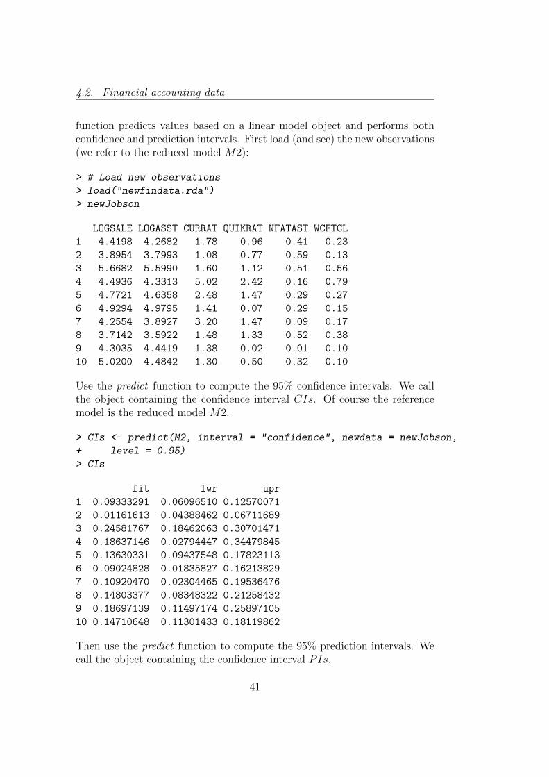
function predicts values based on a linear model object and performs bothconfidence and prediction intervals. First load (and see) the new observations(we refer to the reduced model M2):
> # Load new observations
> load("newfindata.rda")
> newJobson
LOGSALE LOGASST CURRAT QUIKRAT NFATAST WCFTCL
1 4.4198 4.2682 1.78 0.96 0.41 0.23
2 3.8954 3.7993 1.08 0.77 0.59 0.13
3 5.6682 5.5990 1.60 1.12 0.51 0.56
4 4.4936 4.3313 5.02 2.42 0.16 0.79
5 4.7721 4.6358 2.48 1.47 0.29 0.27
6 4.9294 4.9795 1.41 0.07 0.29 0.15
7 4.2554 3.8927 3.20 1.47 0.09 0.17
8 3.7142 3.5922 1.48 1.33 0.52 0.38
9 4.3035 4.4419 1.38 0.02 0.01 0.10
10 5.0200 4.4842 1.30 0.50 0.32 0.10
Use the predict function to compute the 95% confidence intervals. We callthe object containing the confidence interval CIs. Of course the referencemodel is the reduced model M2.
> CIs <- predict(M2, interval = "confidence", newdata = newJobson,
+ level = 0.95)
> CIs
fit lwr upr
1 0.09333291 0.06096510 0.12570071
2 0.01161613 -0.04388462 0.06711689
3 0.24581767 0.18462063 0.30701471
4 0.18637146 0.02794447 0.34479845
5 0.13630331 0.09437548 0.17823113
6 0.09024828 0.01835827 0.16213829
7 0.10920470 0.02304465 0.19536476
8 0.14803377 0.08348322 0.21258432
9 0.18697139 0.11497174 0.25897105
10 0.14710648 0.11301433 0.18119862
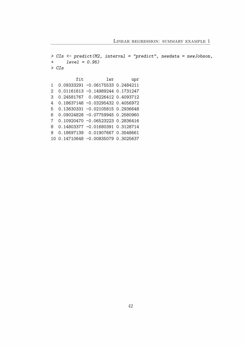
Then use the predict function to compute the 95% prediction intervals. Wecall the object containing the confidence interval PIs.
41
Linear regression: summary example 1
> CIs <- predict(M2, interval = "predict", newdata = newJobson,
+ level = 0.95)
> CIs
fit lwr upr
1 0.09333291 -0.06175533 0.2484211
2 0.01161613 -0.14989244 0.1731247
3 0.24581767 0.08226412 0.4093712
4 0.18637146 -0.03295432 0.4056972
5 0.13630331 -0.02105815 0.2936648
6 0.09024828 -0.07759945 0.2580960
7 0.10920470 -0.06523223 0.2836416
8 0.14803377 -0.01680391 0.3128714
9 0.18697139 0.01907667 0.3548661
10 0.14710648 -0.00835079 0.3025637
42

Chapter 5
Regression diagnostic
5.1 Hat matrix
Think about the regression model:
y = Xβ + e = y + e.
Since β = (XTX)−1XTy, it follows that:
y = Xβ
= X(XTX)−1XTy
= Hy
The matrix H = X(XTX)−1XT is symmetric (H = HT ), idempotent (H ×H = H2 = H) and is called hat matrix, since it ”puts the hat on the y”,namely it provides the vector of the fitted values in the regression of y on X.Let hij (i, j = 1, . . . , n) be the generic element of the H matrix, and let hiidenote its diagonal element. Let X = X−C be the mean deviation from X,where C = 1
n11TX is the centering matrix and 1 is the (n× 1) unit vector.
The hat matrix can be expressed in this alternative way:
H = X(XTX)−1X =1
n11T + X(XTX)−1XT .
It allows to better understand the properties of the hat matrix:
hii = xTi (XTX)−1xi = 1n
+ (xi − x)T (XTX)−1(xi − x).The second term of the expression describes an ellipsoid with center atthe center x. All the points xi that are in the ellipsoid are said to havethe same Mahalanobis distance from x (Jobson, 1991). hii is then large

Regression diagnostic
or small depending on how far xi is away from x. This distance takesinto account the covariance matrix matrix (XTX)−1XT .
When the model is estimated with the intercept,∑n
j=1 hij = 1.
|hij| ≤ 1 ∀i 6= j
When the model is estimated with the intercept 1n≥ hii ≥ 1, otherwise
0 ≥ hii ≥ 1.
hii = 1 iff hij = 0 ∀i 6= j.
If X has full rank, tr(H) = p + 1. It means that the average of hii is(p+ 1)/n.
yi =∑n
j=1 hijyj. It means that each yi is related to all yi through thehij values.
Think about a simple regression model (only one predictor). It can be seenthat
hij =1
n+
(xi − x)(xj − x)∑nj=1(xj − x)2
and
hii =1
n+
(xi − x)2∑nj=1(xj − x)2
.
The further the observation xi is from the center of the data, X, the greaterthe weight placed on the corresponding yj observation in the determinationof yi. Each yj observation has an impact on each value of yi and thus anextreme value of yj influences all yi. The least squares fit is thus very sensitiveto extreme points. It is clear that hii = 1
nwhen xi = x.
The diagonal elements of H, hii, are called leverage. The leverage is a measureof how far the observation xi is from the center of X. When the leverage islarge, yi is more sensitive to changes in yi than when the leverage is relativelysmall. High leverage of y observations corresponds to points where (X− X)is relatively large. Outliers tend to have a large leverage value and hence amajor impact on the predicted values yi.But a high leverage necessarily means problematic observation? Let’s give alook to the following figure.
In Figure 5.1, the point M represents the center of the data (and the pro-jection of the mean of X). The three points N , 0 and D are all distant from
44

5.2. Residuals
Figure 5.1: Leverage, outliers and influence
the main cluster of points with center at M . There is difference among thesepoints? The points 0 and D have large leverage (they are quite far awayfrom M), while the point N yields a leverage equal to 1/n (more or less, itgets a X value extremely close to X). Points 0 and D are distant from thecenter of the data in both the directions, point N is at the mean of the Xvalues but is distant from the Y mean. Suppose to fit a least square line tothe main cluster of data. Suppose to compare the obtained fit with the leastsquares fit including only one of the points 0, D and N . If we include eitherN or 0, both points will have a large influence on the estimated regressionparameters. The slope of the fitted line will change considerably. If we in-clude the point D, it will not have great influence in the estimated regressionparameters: the slope of the regression line will not change at all. ProbablyD is the point with the greater leverage. But it is not a influence point atall. The leverage value is only a partial measure of the impact of observationon the parameters.
5.2 Residuals
A way of judging outliers is to determine whether the extreme point is withina predictable range, given the linear relationship that would be fitted withoutthis extreme point.
45

Regression diagnostic
The residuals from the fitted models are
e = y − y = y −Xβ = (I−H)y,
the residual for the ith observation is then ei = yi − yi.Let’s denote with e(i)i = yi − y(i)i the so-called deleted residual. It is theresidual obtained by taking the difference between the observed yi and theleast squares prediction y(i)i obtained after omitting the point (xi, yi) fromthe least squares fit.
Suppose to have these data, that we call toy 2 data:
y =
8.66239.01997.75198.5500
10.0064
; x =
3.37063.72912.35582.88605.0000
The estimated regression coefficients, the fitted values and the residualsare
β0 = 5.998, β0 = 0.807, y =
8.71929.00877.89988.3279
10.0349
, e =
−0.0569
0.0112−0.1479
0.2221−0.0285
If we re-estimate the model omitting the third observation, we obtainβ0 = 6.349, β1 = 0.724.Hence, y3 = y(i)i = 6.349 + 0.724× 2.3558 = 8.0533.Finally, e(i)i = yi − y(i)i = 7.7519− 8.0533 = −0.3014
The procedure should be delete point i for each i, then refit the model, pre-dict yi obtaining y(i)i and get the residuals e(i)i. Theoretically, we should fitn models to get n deleted residuals. Fortunately, there is a precise relationbetween the residuals of a model and the deleted residuals:
e(i)i =ei
1− hii.
It means that every time we fit a model, we immediately know the deleted
46

5.2. Residuals
residuals for each value.
The hat matrix of the model previously estimated is:
H =
0.2024 0.1936 0.2272 0.2142 0.16260.1936 0.2170 0.1275 0.1620 0.29990.2272 0.1275 0.5094 0.3619 −0.22600.2142 0.1620 0.3619 0.2848 −0.02300.1626 0.2999 −0.2260 −0.0230 0.7865
.
Remember that the residuals of the model are e =
−0.0569
0.0112−0.1479
0.2221−0.0285
. The
diagonal elements of the hat matrix (the leverage points) are hii =0.20240.21700.50940.28480.7865
, with the consequence that
e(i)i =
−0.0569/0.20240.0112/0.2170−0.1479/0.50940.2221/0.2848−0.0285/0.7865
=
−0.0714
0.0143−0.3014
0.3106−0.1335
.Look at the third deleted residual: We get, of course, the same resultpreviously obtained without estimating a new model. We obtain all thedeleted residuals by estimating only one model.
In Figure 5.2, ”a scatterplot of values (xi, yi) is shown with an ordinary leastsquares line y. A second least squares line y(i) denotes the fitted line obtainedafter omitting observation (xi, yi) at point A. The corresponding values of yi,y(i)i, ei and e(i)i are also shown in the figure. In this case the point A appearsto have an impact on the magnitude of the residual” (Jobson 1991, p.152).
As hii is the leverage, it is clear that if the leverage is large for a given pointthen the deleted residual tends to be large for the same point. We expect thatin (large) data sets the omission of a single data point from a least squaresfit should have little impact on the residual for the omitted data point. In
47

Regression diagnostic
Figure 5.2: Residuals and deleted residuals. Figure taken from Jobson, 1991,p.152
other words, we expect that ei and e(i)i are quite similar. Similarly, we expectthat the sum of squared residuals
∑ni=1 e
2i and the sum of squared deleted
residuals∑n
i=1 e2(i)i =
∑ni=1
e2i(1−hii)2 should also be of similar magnitude.
The PRESS (Predicted REsidual Sum of Squares) statistic gives a summarymeasure of the fit of a model to a sample of observations. Probably you willuse this statistics in the future as model selection method (leave-one-out-cross-validation). It is equal to the sum of squared deleted residuals:
PRESS=n∑i=1
e2i(1− hii)2
.
The contribution of each point to the PRESS statistic can be determined,identifying dominant values of e(i)i. Such dominant values can therefore berelated to the leverage values.The ratio of PRESS to the ordinary sum of squared residuals∑n
i=1e2i
(1−hii)2∑ni=1 e
2i
gives an indication of the sensitivity of the fit to omitted observations. Out-liers can often cause this ratio to be much larger than unity.
48

5.2. Residuals
Remember the random variable residuals we introduced in Chapter 3.1.1:
E = Y −XB = Y −X(XTX)−1XTY = (I−H)Y = MY.
We can write:
E = (I−H)Y
= (I−H)(Xβ + ε)
= (I−H)Xβ + (I−H)ε
= Xβ −X(XTX)−1XTXβ + (I−H)ε
= (I−H)ε.
It immediately follows that E[E] = 0 and, by remembering that H is idem-potent and that H ×H = H, var(E) = var((I −H)ε) = (I −H)σ2, hencevar(ei) = σ2(1− hii). This evidence highlights that although the errors mayhave equal variance and be uncorrelated, the residuals do not.Let’s introduced the standardized residuals, known also as internally studen-tized residuals, useful for studying the behavior of the true error terms:
ri =ei
s√
(1− hii).
If the model assumptions are correct var(ri) = 1 and corr(ri, rj) tends to besmall. Any abnormal observation will inevitably affect s, and thus also thestandardized residuals. In the above formulation, we could note that ei isnot independent of s2. Also for this reason, the standardized residuals arecalled internally studentized residuals.
If we were able to compute the sample variance in a model fit without theith observation, then we could obtained a sample variance independent ofthe ith residual.Let s2(i) denote the residual variance after eliminating the i-th observation.The Studentized (or externally Studentized, or Jackknife) residual is definedas
ti =ei
s(i)√
(1− hii).
The externally studentized residual is distributed as a t distribution withn − p − 2 degrees of freedom if the error terms are normal, independent,mean zero and with constant variance. Also in this case we do not have toperform additional regressions because
s2(i) =[(n− p− 1)s2 − e2i /(1− hii)]
n− p− 2.
49

Regression diagnostic
An easy way to compute ti is
ti = ri
(n− p− 2
n− p− 1− r2i
)1/2
i = 1, . . . , n.
The sample variance of the model estimated with toy 2 data is s2 = eT e/(n−p−1) = 0.0754/3 = 0.0251. The PRESS statistic is
∑5i=1 e
2(i)i = 0.2104, while
PRESS/eT e = 2.7911.Let’s compute the standardized (internally studentized) residuals. We have
ri =
−0.0569/(0.1585
√0.7976)
0.0112/(0.1585√
0.7830)
−0.1479/(0.1585√
0.4906)
0.2221/(0.1585√
0.7152)
−0.0285/(0.1585√
0.2135)
=
−0.4022
0.0799−1.3318
1.6568−0.3891
.
If we want compute s2(i), we must compute [(n− p− 1)s2− e2i /(1−hii)]/(n−p− 2) for each observation:
s2(i) =
[3× 0.0251− (−0.05692/0.7976)] /2[3× 0.0251− (0.01122/0.7830)] /2
[3× 0.0251− (−0.14792/0.4906)] /2[3× 0.0251− (0.22212/0.7152)] /2
[3× 0.0251− (−0.02852/0.2135)] /2
=
0.03570.03760.01540.00320.0358
.Then, we are ready to compute ti:
ti =
−0.0569/
√(0.0357 × 0.7976)
0.0112/√
(0.0376 × 0.7830)
−0.1479/√
(0.0154 × 0.4906)
0.2221/√
(0.0032 × 0.7152)
−0.0285/√
(0.0358 × 0.2135)
=
−0.3377
0.0653−1.7009
4.6411−0.3260
.
Of course, we are able to compute ti without computing s2(i), but only knowingri:
ti = ri
(n− p− 2
n− p− 1− r2i
)1/2
=
−0.4022×
√(2/(3− (−0.4022)2))
0.0799×√
(2/(3− (0.0799)2))
−1.3318×√
(2/(3− (−1.3318)2))
1.6568×√
(2/(3− (1.6568)2))
−0.3891×√
(2/(3− (−0.3891)2))
=
−0.3377
0.0653−1.7009
4.6411−0.3260
.
50

5.3. Influence measures
5.3 Influence measures
In a linear regression, a point is an influential point if its deletion, singlyor in combination with others (two or three), causes substantial changes inthe fitted model. Hence, high leverage points need not be influential andinfluential observations are not necessarily high leverage points.Observations with large standardized (or studentized) residuals are outliersin the response variable because they lie far from the fitted equation in thedirection of y. Since the standardized residuals are approximately normallydistributed with mean zero and a standard deviation 1, points with stan-dardized residuals larger than 2 or 3 are called outliers (Chatterjee & Hadi,2005).Outliers in the predictor variables space can also affect the regression results.They are evaluated through the leverage hii. Hence, hii can be used as ameasure of outlyingness in the space of predictors because observations withlarge leverage are to be considered as outliers compared to other points inthe space of the predictors. As the average size of the leverage is (p+1)
n, a way
to consider large a leverage value is to check if hii > 2 (p+1)n
.Hence, there are outliers in the space of y (to be evaluated with standardizedresiduals) and outliers in the space of X (to be evaluated with the leveragevalues).
However, the idea of leverage is all about the potential for an observationto have a large effect on a fitted regression, as well as analyses that are basedon residuals alone may fail to detect outliers and influential observations.First, there is a relationship between leverage and residual so that
hii +ei
σ2/(n− p− 1)≤ 1.
It means that high leverage points tend to have small residuals. Therefore,in addition to an examination of the standardized residuals for outliers, anexamination of the leverage values is also recommended for the identificationof troublesome points.
Second, the use of residuals from a fitted linear relationship to identifyoutliers has the disadvantage that an outlier can mask itself by drawing theline toward itself, as a result the residual is considerably smaller than itwould have been had this point been omitted from the data set (swampingphenomenon). The masking phenomenon occurs when the data contain out-liers, but we fail to detect them: some of the outliers may be hidden by otheroutliers in the data.
51

Regression diagnostic
For this reason, several measures of influence of observations have been pro-posed.
5.3.1 Cook’s distance
The Cook’s distance combines the notions of outlyingness and leverage. Forthe ith observation, it is defined as
Di =(yi − y(i)i)T (yi − y(i)i)
s2(p+ 1)
=(β(i) − β
)T(XTX)
(β(i) − β
)/s2(p+ 1)
=
[hii
1− hii
]e2i
(p+ 1)s2(1− hii)
=
[hii
1− hii
]r2i
(p+ 1)
=
hii
1− hii
r2i( 1
p+ 1
),
where yi and β are the fitted value and the estimated vector of regressioncoefficients in a model that includes the ith observation, and y(i)i and β(i)
are the prediction of the ith observation and the least squares estimate of βwithout the ith observation.The Cook’s distance measures the difference between the fitted values ob-tained from the full data and the fitted values obtained by deleting the ithobservation. If we better give a look to the last term of the equation,
Di =
hii
1− hii
r2i( 1
p+ 1
),
we can note that Cook’s distance is a multiplicative function of two basicquantities (Draper & Smith, 1998, p.212): the ratio (variance of the ithpredicted value)/(variance of the ith residual), also called potential function,and the squared standardized residual. Remember that in Chapter 3.3 wedefined the variance of the predicted value as var(y) = s2H, then it is clearthat var(yi) = s2hii. The variance of the ith residual is, as we know, equalto s2(1− hii).Di will be large if the (squared) standardized residual is large and/or if theleverage is large. We know that observations with large absolute standardizedresidual or leverage points are potentially influential: points that are bothare the most influential. High Di values indicate influential observations
52

5.3. Influence measures
on the vector of β parameters. As a rule of thumb, points with Di valuesgreater than 1 could be classified as being influential. Really often, it isbetter evaluate the Cook’s distance graphically through a, say, dot plot thanevaluating each single point using a rigid rule.
5.3.2 The DF family
The influence measures belonging to the so called DF (Difference in) familyare somewhat related to the Cook’s distance. Let’s start with the DFFITS(Difference to fit):
DFFITSi =(yi − y(i)i)s(i)√hii
= ti
√[hii
1− hii
]This measure is the difference between the ith fitted value obtained fromthe full data and the ith fitted value obtained by deleting the ith observa-tion scaled by s(i)
√hii. Points with DFFITS > 2
√pn
need to be investi-gated. Also in this case, instead of having a strict cutoff value, generally theDFFITS are used in a graph (dot plot, boxplot, etc) to detect points ofabnormally high influence relative to other points. Generally, the informa-tion given by the DFFITS are equivalent to the ones given by the Cook’sdistance.
Let β be the vector of regression coefficients and let β(i) be the vector ofregression coefficients after extracting the ith observation in the data. Thequantity
DB = β − β(i) =(XTX)−1xi
T ei(1− hii)
measures the difference in each parameter estimate with and without ithpoint. Let β(j)i be the estimate of the jth regression coefficient after deletingthe ith observation. The DFBETA (Difference in beta) measure is definedas
DFBETAj,i =βj − βj(i)
s(i)√
(XTX)−1(jj)
,
where the subscript (jj) denotes the diagonal element of the matrix (XTX)−1
corresponding to βj. The DFBETA measures the difference in each parame-
53

Regression diagnostic
ter estimate with and without the potential influential point. Of course, thereexist a DFBETA for each predictor and for each observation. Points withDFBETAj,i >
2√n
(or sometimes greater than 1) need to be investigated.
5.3.3 Hadi’s influence measure
The Hadi’s influence measure (Hadi, 1992) takes in account that an obser-vation can be a potential influence point because it can be an outlier eitherin the space of y or in the space of X, or in both spaces. The measure isdefined as
H2i =
(hii
1− hii
)+
(p+ 1
1− hiie2i
eT e− e2i
)=
(hii
1− hii
)+
(p+ 1
1− hiid2i
1− d2i
),
where d2i = e2i /eT e. As it can be noticed, H2
i is additively composed bytwo terms: the first one is the potential function that measures outlyingnessin the X-space, the second one is function of the residuals and measuresoutlyingness in the y-space.
5.3.4 Covariance ratio
The Covariance Ratio measures the impact of the ith observation on thevariances and covariances among the coefficients. Omitting xi from the re-gression causes differences in the summations in determining the covariancematrix.The ratio of the determinants of the new covariance matrix to the originalcovariance matrix is called COVRATIO.
COV RATIOi =|s2(i)(XT
(i)X(i))−1|
|s2(XTX)−1|
=(n− p)p
[(n− p− 1) + ti]p (1− hii)
If |COV RATIOi−1| > 3p/n, then the ith observation causes a large changein the covariance for β.
54
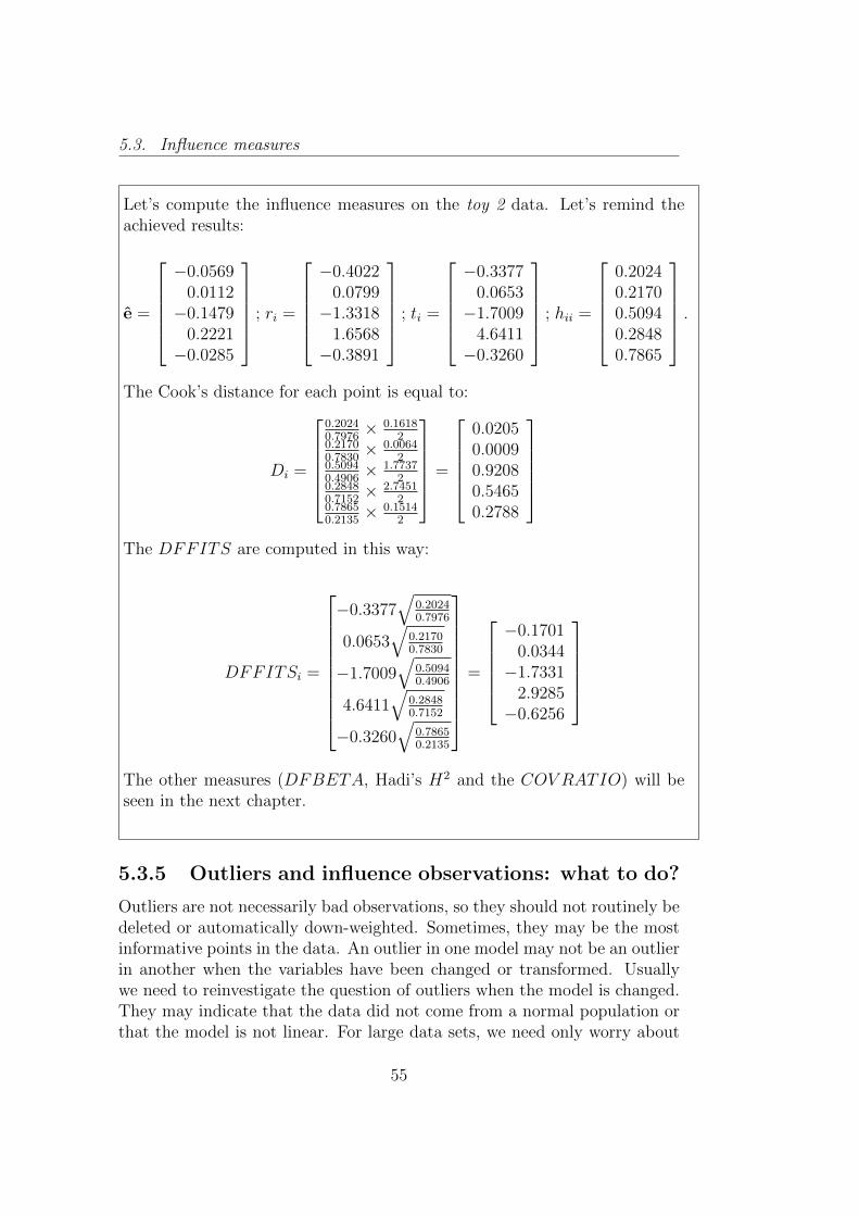
5.3. Influence measures
Let’s compute the influence measures on the toy 2 data. Let’s remind theachieved results:
e =
−0.0569
0.0112−0.1479
0.2221−0.0285
; ri =
−0.4022
0.0799−1.3318
1.6568−0.3891
; ti =
−0.3377
0.0653−1.7009
4.6411−0.3260
; hii =
0.20240.21700.50940.28480.7865
.The Cook’s distance for each point is equal to:
Di =
0.20240.7976
× 0.16182
0.21700.7830
× 0.00642
0.50940.4906
× 1.77372
0.28480.7152
× 2.74512
0.78650.2135
× 0.15142
=
0.02050.00090.92080.54650.2788
The DFFITS are computed in this way:
DFFITSi =
−0.3377√
0.20240.7976
0.0653√
0.21700.7830
−1.7009√
0.50940.4906
4.6411√
0.28480.7152
−0.3260√
0.78650.2135
=
−0.1701
0.0344−1.7331
2.9285−0.6256
The other measures (DFBETA, Hadi’s H2 and the COV RATIO) will beseen in the next chapter.
5.3.5 Outliers and influence observations: what to do?
Outliers are not necessarily bad observations, so they should not routinely bedeleted or automatically down-weighted. Sometimes, they may be the mostinformative points in the data. An outlier in one model may not be an outlierin another when the variables have been changed or transformed. Usuallywe need to reinvestigate the question of outliers when the model is changed.They may indicate that the data did not come from a normal population orthat the model is not linear. For large data sets, we need only worry about
55

Regression diagnostic
clusters of outliers. Such clusters are less likely to occur by chance and theytend to represent more likely the actual structure. Finding these cluster isnot always easy.Always data entries should checked for error first. These are relatively com-mon. Moreover, the physical context should be examined: sometimes, thediscovery of an outlier may be of singular interest. For example, in the sta-tistical analysis of credit card transactions outliers may represent fraudulentuse. If the point from the analysis is excluded, any suggestion of dishonestyshould be avoided: the existence of outliers must always been reported evenif they are not included in the final model.
Summarizing, outliers and influential observations can be the most in-formative observations in the data set. They should be examined to deter-mine why they are outlying or influential. Appropriate corrective actionscan then be taken, including: correction of error in the data, deletion ordown-weighing outliers, transforming the data (probably you will study theBox-Cox transformation), considering a different model (probably you willstudy the polynomial regression), redesigning the experiment or the samplesurvey, collecting more data.
5.4 Diagnostic plots
qqplot
A plot commonly used in regression diagnostic is the qqplot (quantile-quantileplot). A qqplot is generally designed to see if the quantiles of two distribu-tions sufficiently match by plotting their quantiles against each other. If ei,1 ≤ i ≤ n were really a sample drawn fromN (0, σ2), then their sample quan-tiles should be close to the theoretical quantiles of the N (0, σ2) distribution.The qqplot is then a plot of e(i) vs. E(ε(i)), 1 ≤ i ≤ n, where e(i) is the i-thsmallest residual(order statistic) and E(ε(i)) is the expected value for inde-pendent εi’s ∼ N (0, σ2). If the two compared distributions are similar, thepoints in the plot will approximately lie on the line y = x. Moreover, theqqplot can be useful to detect the linear relation between the two distribu-tions if the points will approximately lie on a line, although not the line forwhich y = x.Figure 5.3 shows two qqplots where on the horizontal axis the theoreticalquantiles of a standard normal distribution are represented.
In panel (a), 125 randomly data generated from a standard normal distri-bution on the vertical axis are compared to a standard normal population
56

5.4. Diagnostic plots
−2 −1 0 1 2
−2
−1
01
2
Q−Q plot
Theoretical Quantiles N(0,1)
Sam
ple
quan
tiles
(a)
−2 0 2 4
−2
02
4
Q−Q plot
Theoretical Quantiles N(0,1)
Sam
ple
quan
tiles
(b)
Figure 5.3: qqplot for 125 random draws from a standard normal distribution(a) and for 125 random draws from a exponential distribution with λ = 1.3(b)
57

Regression diagnostic
on the horizontal axis. The linearity of the points suggests that the dataare normally distributed. In panel (b)125 randomly data generated from anexponential distribution with parameter λ = 1.3 on the vertical axis are com-pared to a standard normal population on the horizontal axis. The pointsfollow a strongly nonlinear pattern, suggesting that the data are not dis-tributed as a standard normal.
Fitted vs Residuals
The fitted versus residuals plot is a scatter plot of residuals, both raw andstudentized, on the vertical axis and fitted values on the vertical axis. Theplot is useful to detect non-linearity, heteroscedasticity, and outliers.
Figure 5.4: Fitted vs residual plot
Figure 5.4 shows two examples of fitted vs residuals plot. In general,equally spread residuals around a horizontal line without distinct patternsare a good indication you don’t have non-linear relationships. The case-1plot shows a ”good” model, the case-2 plot shows a ”bad” model.
58

5.5. Multicollinearity
Figure 5.5 shows two examples of fitted vs residuals plot where heteroscedas-ticity (left panel) or non-linearity (right panel) are detected. If all is well,you should see constant variance in the vertical (e) direction and the scattershould be symmetric vertically about 0.
Figure 5.5: Fitted vs residual plot
In these cases, the problems are evident because the range of the residu-als is changing over the horizontal axis on the left, denoting possible het-eroscedasticity, as well as on the right residuals are not randomly and sym-metrically placed around their mean. In this latter case, apart from possiblenon-linearity, also correlation among residuals could be detected.
5.5 Multicollinearity
The term multicollinearity refers to the situation in which two of morecolumns of the X matrix are linear combinations of each other, or whenthey are very close to be linearly correlated. In the first case, the problem isnot a big problem: X has not full rank and then the matrix (XTX) has notinverse, so the OLS estimator does not exist. The solution is remove somepredictors and estimate the model. In the second case, technically X has fullrank, so the OLS solution exists. In this situation, the coefficient estimates ofthe multiple regression may change erratically in response to small changesin the model or the data.Let us see the consequences of multicollinearity. Although BLUE, the OLS
59

Regression diagnostic
estimators posses large standard errors, which means the coefficients cannotbe estimated with great precision. Because of large standard errors, boththe the confidence intervals tend to be larger and t ratio for one or moreregressors tends to be statistically not significant (they tends to be small).Nevertheless, it may occurs that goodness of fit measures can be high suggest-ing a good model. OLS estimators and their standard errors can be sensitiveto small changes in the data.Suppose that x1 and x2 are two predictors that are correlated in the contextof a general regression model. Normally, the regression coefficient measuresof the effect of a one unit change in x1 holding the other variables constant.If x1 and x2 are correlated, we may not have a set of observations for whichall changes in x1 are independent of changes in x2, then we have impreciseestimates of the effect of changes in x1. In a few words, multicollinearitymeans unstable estimated regression coefficients. Note that eventual multi-collinearity problems are not miss-specification problems.
5.5.1 Measures of multicollinearity detection
There exist several indexes devoted to the detection of the multicollinearity.We will examine some of them.
VIF
The relationship between the predictor variables can be judged by examininga quantity called the variance inflation factor (VIF). The index is computedby regressing each of the xj variables on remaining x variables and findingout the corresponding coefficients of determination R2
j . A high R2j would
suggest that xj is highly correlated with the rest of the x’s. The VIF forvariable xj is
V IFj =1
1−R2j
.
If xj has a strong linear relationship with the other predictor variables, thenR2j is close to 1 and the ratio is large. If instead there is not linear relationship
between the predictor variables, and then they are orthogonal, R2j is close to
zero and V IFj tends to one. The deviation of VIF values from 1 indicatesdeparture from orthogonality and tendency toward collinearity. In practicalcases, if there are VIF values greater than 10, then we say that the data havecollinearity problems.
60

5.5. Multicollinearity
Tolerance
The denominator of the VIF index, 1 − R2j , is called tolerance. Some soft-
ware uses the tolerance as multicollinearity detection index. Of course, itgives the same information of the VIF. Tolerance measures less than 0.1 in-dicate collinearity problems. VIF and tolerance are related, of course, to thecorrelation structure of the predictors.
Let R be the p × p correlation matrix of the p predictors. The diagonalelements of the inverse of R coincide with the VIF:
diag(R−1) =1
1−R2j
.
Condition number and condition index
Usually, models are estimated with the intercept term. It is usual to scalethe X matrix by dividing each column of X by the sum of squared values ofthe column itself, then we can proceed with the cross-product of the scaledX. In other words, let Xs be a n × (p + 1) matrix in which for each of thej = 1, . . . , p+ 1 column we compute by xj/
∑xi=1 x
2ji, the matrix T = XT
s Xs
is computed. The same matrix can be computed in this way:
T = D−1(XTX)D−1,
where D is a diagonal matrix containing the square root of the diagonalelements of (XTX).
As the (p+ 1)× (p+ 1) matrix T is a positive definite symmetric matrix(it has 1 on the diagonal, exactly as the correlation matrix has), it can bewritten as the product of these matrices, T = VΛVT .Λ is a diagonal matrix of unique non-negative elements called eigenvalues,denoted by λj, j = 1, . . . , p, usually ordered in increasing order.V is a p×p orthogonal matrix (VVT = VTV = I, VT = V−1). The columnsof V are called eigenvectors, sharing a one-to-one correspondence with theeigenvalues.As the rank of T is equal to
∑(j=1 p+ 1)λj, it is clear that if an eigenvalue is
equal to zero, then there is perfect linear dependence. Then, an eigenvalueclose to zero indicates a near linear dependency. Given these considerations,it becomes clear the definition of the collinearity indexes based on the eigen-structure of the scaled crossproduct matrix. The condition number is definedas
CN =λmaxλmin
,
61

Regression diagnostic
namely the ratio between the maximum and the minimum eigenvalue. Asa rule of thumb, a CN between 100 and 1000 reports a moderate to strongmulticollinearity. If CN exceeds 1000, then there is severe multicollinearity.Some statistical software reports the condition index, defined as
CI =
√λmaxλmin
=√CN,
namely simply the square root of the condition number. The rule of thumbsare essentially the same: a CI between 10 and 30 reports a moderate to strongmulticollinearity. If CI exceeds 30, then there is severe multicollinearity.
If a model has been estimated without the intercept, sometimes the cor-relation matrix R is used instead of T.
Variance proportion
Recall the sample covariance matrix of the OLS estimator:
var(β) = s2(XTX)−1.
Hence, as XTX = VΛVT (eigenvalues and eigenvectors can be computed foreach square matrix), we have that
var(β) = s2(VΛVT )−1 = s2VΛ−1VT ,
meaning that
var(βk) = s2p+1∑j=1
v2kjλj.
The variance of each regression coefficient can be decomposed into a sum ofcomponents, each associated with one and only one of the (p + 1) eigeval-ues. Hence, those components associated with near dependencies (namely,with small λi) will be large relative to the other components. Then, unusu-ally high proportion of the variance of two or more coefficients concentratedin components associated with the same small eigenvalue provides evidencethat the corresponding near dependency is causing problems (Belsley, Kuh& Welsch, 2005).The k, j variance proportion is the proportion of the variance of the kthregression coefficient associated with the jth component (eigenvalue) of its
62

5.5. Multicollinearity
decomposition:
mjk =
v2kjλj∑p+1j=1
v2kjλj
.
Results are generally reported in a table such the following one:
λ CIVariance proportion of
β0 β1 . . . βp
λ1
√λ1λ1
v21,1/λ1
(v21,1/λ1)+(v21,2/λ2)+...+(v21,(p+1)
/λp+1)
v22,1/λ1
(v22,1/λ1)+(v22,2/λ2)+...+(v22,(p+1)
/λp+1). . .
v2(p+1),1
/λ1
(v2(p+1),1
/λ1)+(v2(p+1),2
/λ2)+...+(v2(p+1),(p+1)
/λp+1)
λ2
√λ1λ2
v21,2/λ2
(v21,1/λ1)+(v21,2/λ2)+...+(v21,(p+1)
/λp+1)
v22,2/λ2
(v22,1/λ1)+(v22,2/λ2)+...+(v22,(p+1)
/λp+1). . .
v2(p+1),2
/λ1
(v2(p+1),1
/λ1)+(v2(p+1),2
/λ2)+...+(v2(p+1),(p+1)
/λp+1)
. . . . . . . . . . . . . . . . . .
λp+1
√λ1λp+1
v21,(p+1)
/λ(p+1)
(v21,1/λ1)+(v21,2/λ2)+...+(v21,(p+1)
/λp+1)
v22,(p+1)
/λ(p+1)
(v22,1/λ1)+(v22,2/λ2)+...+(v22,(p+1)
/λp+1). . .
v2(p+1),(p+1)
/λ1
(v2(p+1),1
/λ1)+(v2(p+1),2
/λ2)+...+(v2(p+1),(p+1)
/λp+1)
In the table above, vi,j represents the entry of the eigenvector, and λ1, . . . , λp+1
are the eigenvalues placed in decreasing order. In practical cases, the eigen-vectors and the eigenvalues are computed from the matrix T as above intro-duced.For each regression coefficient, its variance is distributed to the differenteigenvalues, the variance proportions adding up to one column by column.For each row in the table with a high Condition Index, values above 0.90 inthe variance proportions are searched for. Two or more values above thisthreshold in one line highlight that there is a collinearity problem betweenthose predictors. If only one predictor in a line has a value above 0.90, thisis not a sign for multicollinearity.
Summarizing, the diagnostic procedure for multicollinearity is the following(Belsley, Kuh & Welsch, 2005, p. 112):
1. A eigenvalue associated with a high condition index;
2. High variance-decomposition proportions for two or more estimatedregression coefficient.
The number of condition indexes deemed large (say, greater than 30)sub 1 identifies the number of near dependencies among the columns ofthe data matrix. Furthermore, the determination sub 2 of large variance-decomposition proportions (say, greater than 0.9) associated with each highcondition index identifies those variates that are involved in the correspond-ing near dependency, and the magnitude of these proportions in conjunctionwith the high condition index provides a measure of the degree to whichthe corresponding regression estimate has been degraded by the presence of
63

Regression diagnostic
collinearity.
Sometimes, for models estimated without the intercept, instead of using ma-trix T the computations are made by starting from the correlation matrixR.
64

5.5. Multicollinearity
Let’s add a variable, we call X3, to the toy example introduced in Chapter 2.3.1:
X =
16.11 7 3.3114.72 3 1.8916.02 4 2.3315.05 4 3.8416.58 4 4.2815.22 8 2.6913.95 3 4.8514.71 9 4.9115.48 9 4.3613.78 3 4.99
.
In order to compute the VIF, we must estimate three regression models (x1 =β0 + βx2x2 + βx3x3, x2 = β0 + βx1x1 + βx3x3 and x3 = β0 + βx1x1 + βx2x2) andthen compute the three R2. Note that the models must be estimated with theintercept. The three matrix of predictors are
X1 =
1 7 3.311 3 1.891 4 2.331 4 3.841 4 4.281 8 2.691 3 4.851 9 4.911 9 4.361 3 4.99
; X2 =
1 16.11 3.311 14.72 1.891 16.02 2.331 15.05 3.841 16.58 4.281 15.22 2.691 13.95 4.851 14.71 4.911 15.48 4.361 13.78 4.99
; X3 =
1 16.11 71 14.72 31 16.02 41 15.05 41 16.58 41 15.22 81 13.95 31 14.71 91 15.48 91 13.78 3
.
Compute the necessary quantities as exercise. You will get R2x1 = 0.23, R2
x2 = 0.12and R2
x3 = 0.19. Tolerances are then 1 − 0.23 = 0.77, 1 − 0.12 = 0.88 and1 − 0.19 = 0.81. Hence the VIFs are equal to 1/0.77 = 1.31, 1/0.88 = 1.13 and1/0.81 = 1.23.
The correlation matrix of X and its inverse are
R =
1.00 0.26 −0.380.26 1.00 0.11−0.38 0.11 1.00
; R−1 =
1.31 −0.40 0.54−0.40 1.13 −0.28
0.54 −0.28 1.23
Note that the diagonal elements of R−1 correspond to the VIFs.
65

Regression diagnostic
Let’s compute the condition number, the condition index and the varianceproportion. We begin with the most common case in which we estimate the modelwith the intercept (so add a column of one to X). Hence, first we compute thematrix T = D−1/2XTXD−1/2. We have
XTX =
10 151.62 54.00 37.46
152 2306.31 824.17 564.4154 824.17 350.00 205.1737 564.41 205.17 151.85
; D−1/2 =
0.316 0.000 0.000 0.0000.000 0.021 0.000 0.0000.000 0.000 0.053 0.0000.000 0.000 0.000 0.081
.Hence
T =
0.316 0.000 0.000 0.0000.000 0.021 0.000 0.0000.000 0.000 0.053 0.0000.000 0.000 0.000 0.081
×
10 151.62 54.00 37.46152 2306.31 824.17 564.4154 824.17 350.00 205.1737 564.41 205.17 151.85
×
0.316 0.000 0.000 0.0000.000 0.021 0.000 0.0000.000 0.000 0.053 0.0000.000 0.000 0.000 0.081
=
1.000 0.998 0.913 0.9610.998 1.000 0.917 0.9540.913 0.917 1.000 0.8900.961 0.954 0.890 1.000
Eigenvalues and eigenvectors of T are
Λ =
3.818 0.000 0.000 0.0000.000 0.126 0.000 0.0000.000 0.000 0.055 0.0000.000 0.000 0.000 0.001
; V =
−0.507 0.256 −0.386 0.726−0.507 0.202 −0.485 −0.683−0.487 −0.866 0.113 0.026−0.498 0.380 0.776 −0.069
The condition number is CN = λmax/λmin = 3.818/0.001 = 3246.040. The con-
dition index is CI =√CN = 56.974.
In order to compute the variance proportion, we need to compute mjk =
v2kjλj∑p+1
j=1
v2kjλj
.
66

5.5. Multicollinearity
First, let’s compute the first column of the variance proportions table. It containsthe condition indexes, hence
CI1 =
√3.818
3.818= 1; CI2 =
√3.818
0.126= 5.506; CI3 =
√3.818
0.126= 8.318; CI4 =
√3.818
0.126= 56.974.
Then we must compute the variance proportions. These are, for the intercept term(mk,j , with k = 1, namely the first regression parameter that in this case is theintercept), m1,1, m1,2, m1,3, and m1,4. Hence
m1,1 =v21,1/λ1
(v1,1/λ1) + (v1,2/λ2) + (v1,3/λ3) + (v1,4/λ4)
=−0.50742/3.8177
(−0.50742/3.8177) + (0.25632/0.1259) + (−0.38622/0.0552) + (0.72642/0.0012)= 0.0001
m2,1 =v21,2/λ2
(v1,1/λ1) + (v1,2/λ2) + (v1,3/λ3) + (v1,4/λ4)
=0.25632/0.1259
(−0.50742/3.8177) + (0.25632/0.1259) + (−0.38622/0.0552) + (0.72642/0.0012)= 0.0012
m3,1 =v21,3/λ3
(v1,1/λ1) + (v1,2/λ2) + (v1,3/λ3) + (v1,4/λ4)
=−0.38622/0.0552
(−0.50742/3.8177) + (0.25632/0.1259) + (−0.38622/0.0552) + (0.72642/0.0012)= 0.0060
m4,1 =v21,4/λ4
(v1,1/λ1) + (v1,2/λ2) + (v1,3/λ3) + (v1,4/λ4)
=0.72642/0.0012
(−0.50742/3.8177) + (0.25632/0.1259) + (−0.38622/0.0552) + (0.72642/0.0012)= 0.9927
The complete table is then
CI β0 β1 β2 β31.0000 0.0001 0.0002 0.0091 0.00405.5064 0.0012 0.0008 0.8754 0.07058.3176 0.0060 0.0106 0.0341 0.6729
56.9740 0.9927 0.9884 0.0814 0.2526
67

Regression diagnostic
In the case in which the model is estimated without intercept, the T matrix is 1.00000 0.91733 0.953730.91733 1.00000 0.889960.95373 0.88996 1.00000
,Λ and V are
Λ =
2.84093 0.00000 0.000000.00000 0.11645 0.000000.00000 0.00000 0.04262
, V =
0.58364 0.23764 0.776460.57028 −0.80067 −0.183610.57806 0.54996 −0.60283
.The variance proportion table is
CI β1 β2 β31.0000 0.0081 0.0179 0.01054.9393 0.0329 0.8588 0.23118.1640 0.9590 0.1234 0.7585
*****
If the model is estimated without intercept and the computations have to be madeon the correlation matrix R, we have
R =
1.0000 0.2597 −0.37730.2597 1.0000 0.1116−0.3773 0.1116 1.0000
,and
Λ =
1.4112 0.0000 0.00000.0000 1.1034 0.00000.0000 0.0000 0.4854
; V =
−0.7414 0.0965 0.6641−0.3060 0.8321 −0.4625
0.5973 0.5461 0.5874
.The variance proportion table is
CI β1 β2 β31.0000 0.2981 0.0585 0.20491.1309 0.0065 0.5531 0.21911.7050 0.6954 0.3885 0.5760
As exercise, Check by yourself the results obtained in this page.
68
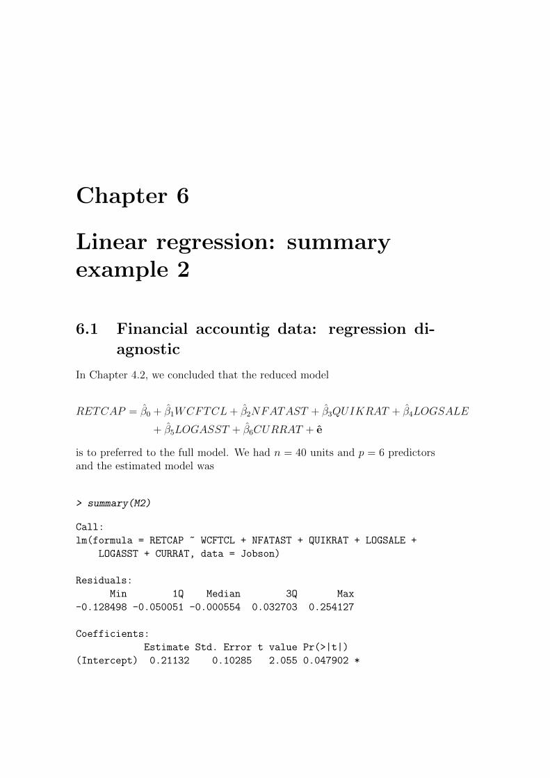
Chapter 6
Linear regression: summaryexample 2
6.1 Financial accountig data: regression di-
agnostic
In Chapter 4.2, we concluded that the reduced model
RETCAP = β0 + β1WCFTCL+ β2NFATAST + β3QUIKRAT + β4LOGSALE
+ β5LOGASST + β6CURRAT + e
is to preferred to the full model. We had n = 40 units and p = 6 predictorsand the estimated model was
> summary(M2)
Call:
lm(formula = RETCAP ~ WCFTCL + NFATAST + QUIKRAT + LOGSALE +
LOGASST + CURRAT, data = Jobson)
Residuals:
Min 1Q Median 3Q Max
-0.128498 -0.050051 -0.000554 0.032703 0.254127
Coefficients:
Estimate Std. Error t value Pr(>|t|)
(Intercept) 0.21132 0.10285 2.055 0.047902 *

Linear regression: summary example 2
WCFTCL 0.42488 0.05866 7.243 2.62e-08 ***
NFATAST -0.50515 0.07470 -6.762 1.04e-07 ***
QUIKRAT 0.08335 0.04130 2.018 0.051768 .
LOGSALE 0.09764 0.02506 3.896 0.000451 ***
LOGASST -0.07095 0.03234 -2.194 0.035387 *
CURRAT -0.12210 0.04062 -3.006 0.005034 **
---
Signif. codes: 0 '***' 0.001 '**' 0.01 '*' 0.05 '.' 0.1 ' ' 1
Residual standard error: 0.07455 on 33 degrees of freedom
Multiple R-squared: 0.741, Adjusted R-squared: 0.6939
F-statistic: 15.74 on 6 and 33 DF, p-value: 1.927e-08
6.1.1 Residuals analysis
First, let’s extract the residuals from the model.
> M2e <- M2$residuals
> M2e
1 2 3 4 5
0.068564894 0.254126514 0.075008752 0.105252987 0.004129011
6 7 8 9 10
-0.006275451 0.004366316 0.062720493 -0.057296326 0.045175534
11 12 13 14 15
-0.069948478 -0.021604108 0.051478822 0.025221913 -0.089565792
16 17 18 19 20
0.018885703 0.025809093 -0.005975702 0.030375129 -0.128497973
21 22 23 24 25
-0.056153901 -0.057198521 0.015491733 -0.060878199 -0.017969721
26 27 28 29 30
0.073744624 -0.122663332 -0.041246557 -0.027177425 0.039686181
31 32 33 34 35
-0.048421916 -0.073580907 0.014615622 -0.019247645 -0.002237348
36 37 38 39 40
0.064824082 -0.041224332 -0.054936399 0.021492498 0.001130134
Then we can use the function hatvalues() to extract the diagonal elementsof the hat matrix.
> M2hii <- hatvalues(M2)
> M2hii
1 2 3 4 5
0.20881538 0.13053172 0.37582276 0.04309421 0.05688139
6 7 8 9 10
0.16389662 0.45587156 0.07841167 0.09644119 0.23039548
11 12 13 14 15
0.05977878 0.16607358 0.47579968 0.07425559 0.22311568
16 17 18 19 20
0.90279169 0.05981985 0.04456994 0.09144512 0.07512527
21 22 23 24 25
0.85483218 0.04889379 0.11494809 0.05685606 0.07027106
70

6.1. Financial accountig data: regression diagnostic
26 27 28 29 30
0.17960245 0.18544850 0.03479675 0.06707152 0.06479273
31 32 33 34 35
0.06075682 0.08251295 0.32568026 0.03893353 0.32518014
36 37 38 39 40
0.12513148 0.08560090 0.07803595 0.11797067 0.06974700
We can arrange both e and hii in two columns with the function cbind,which is a function that takes a sequence of vector, matrix or data-framearguments and combines them by columns. We also define a vector called idthat will help us to easily identify the statistical units:
> #generate a sequence of integers from 1 to 40
> id <- seq(min=1,max=40)
> #combine the three objects in three columns
> M2t1 <- cbind(id, M2e,M2hii)
> M2t1
id M2e M2hii
1 1 0.068564894 0.20881538
2 1 0.254126514 0.13053172
3 1 0.075008752 0.37582276
4 1 0.105252987 0.04309421
5 1 0.004129011 0.05688139
6 1 -0.006275451 0.16389662
7 1 0.004366316 0.45587156
8 1 0.062720493 0.07841167
9 1 -0.057296326 0.09644119
10 1 0.045175534 0.23039548
11 1 -0.069948478 0.05977878
12 1 -0.021604108 0.16607358
13 1 0.051478822 0.47579968
14 1 0.025221913 0.07425559
15 1 -0.089565792 0.22311568
16 1 0.018885703 0.90279169
17 1 0.025809093 0.05981985
18 1 -0.005975702 0.04456994
19 1 0.030375129 0.09144512
20 1 -0.128497973 0.07512527
21 1 -0.056153901 0.85483218
22 1 -0.057198521 0.04889379
23 1 0.015491733 0.11494809
24 1 -0.060878199 0.05685606
25 1 -0.017969721 0.07027106
26 1 0.073744624 0.17960245
27 1 -0.122663332 0.18544850
28 1 -0.041246557 0.03479675
29 1 -0.027177425 0.06707152
30 1 0.039686181 0.06479273
31 1 -0.048421916 0.06075682
32 1 -0.073580907 0.08251295
33 1 0.014615622 0.32568026
34 1 -0.019247645 0.03893353
35 1 -0.002237348 0.32518014
36 1 0.064824082 0.12513148
71

Linear regression: summary example 2
37 1 -0.041224332 0.08560090
38 1 -0.054936399 0.07803595
39 1 0.021492498 0.11797067
40 1 0.001130134 0.06974700
As the average size of the leverage measure is (p+1)/n, a way to consider largea leverage value is to check if hii > 2(p + 1)/n. Here we have 7/40 = 0.175,then the ”critical value” is 2 × 0.175 = 0.35. Observations number 16 and21 have a quite large leverage (hii > 0.8). Observations number 3, 7 and 13have a leverage larger than the critical point.
We can use the functions rstandard() and rstudent() to compute the stan-dardized (or internally studentized) and studentized (or externally studen-tized, or jackknife) residuals. We can arrange these results in columns againwith the function cbind adding two columns to the M2t1 object:
> #standardized residuals
> M2ri <- rstandard(M2)
> #studentized residuals
> M2ti <- rstudent(M2)
> #add two columns to matrix M2t1
> M2t1 <- cbind(M2t1,M2ri,M2ti)
> M2t1
id M2e M2hii M2ri M2ti
1 1 0.068564894 0.20881538 1.03398845 1.03510717
2 1 0.254126514 0.13053172 3.65574507 4.66691187
3 1 0.075008752 0.37582276 1.27353466 1.28609299
4 1 0.105252987 0.04309421 1.44328678 1.46834967
5 1 0.004129011 0.05688139 0.05703162 0.05616362
6 1 -0.006275451 0.16389662 -0.09205932 -0.09066540
7 1 0.004366316 0.45587156 0.07939941 0.07819460
8 1 0.062720493 0.07841167 0.87638267 0.87322358
9 1 -0.057296326 0.09644119 -0.80853972 -0.80420041
10 1 0.045175534 0.23039548 0.69075222 0.68517720
11 1 -0.069948478 0.05977878 -0.96764497 -0.96668385
12 1 -0.021604108 0.16607358 -0.31734032 -0.31297306
13 1 0.051478822 0.47579968 0.95374605 0.95240220
14 1 0.025221913 0.07425559 0.35162947 0.34691127
15 1 -0.089565792 0.22311568 -1.36306570 -1.38171403
16 1 0.018885703 0.90279169 0.81252033 0.80824028
17 1 0.025809093 0.05981985 0.35704257 0.35227229
18 1 -0.005975702 0.04456994 -0.08200536 -0.08076153
19 1 0.030375129 0.09144512 0.42745986 0.42210360
20 1 -0.128497973 0.07512527 -1.79228725 -1.85765077
21 1 -0.056153901 0.85483218 -1.97695851 -2.07342571
22 1 -0.057198521 0.04889379 -0.78672525 -0.78208242
23 1 0.015491733 0.11494809 0.22088613 0.21767460
24 1 -0.060878199 0.05685606 -0.84086369 -0.83704102
25 1 -0.017969721 0.07027106 -0.24998616 -0.24640277
26 1 0.073744624 0.17960245 1.09212157 1.09542532
27 1 -0.122663332 0.18544850 -1.82309072 -1.89311980
28 1 -0.041246557 0.03479675 -0.56315910 -0.55724493
72

6.1. Financial accountig data: regression diagnostic
29 1 -0.027177425 0.06707152 -0.37743045 -0.37247262
30 1 0.039686181 0.06479273 0.55047572 0.54457708
31 1 -0.048421916 0.06075682 -0.67020203 -0.66450721
32 1 -0.073580907 0.08251295 -1.03042874 -1.03142492
33 1 0.014615622 0.32568026 0.23874658 0.23530468
34 1 -0.019247645 0.03893353 -0.26336235 -0.25961429
35 1 -0.002237348 0.32518014 -0.03653360 -0.03597653
36 1 0.064824082 0.12513148 0.92964637 0.92768064
37 1 -0.041224332 0.08560090 -0.57828047 -0.57235865
38 1 -0.054936399 0.07803595 -0.76746043 -0.76257881
39 1 0.021492498 0.11797067 0.30697159 0.30271724
40 1 0.001130134 0.06974700 0.01571745 0.01547753
Note that observations 2 and 21 have |ti| > 0.2. Of course, we can visualizethe, say, studentized residuals by writing
> M2ti
1 2 3 4 5 6 7 8
1.03510717 4.66691187 1.28609299 1.46834967 0.05616362 -0.09066540 0.07819460 0.87322358
9 10 11 12 13 14 15 16
-0.80420041 0.68517720 -0.96668385 -0.31297306 0.95240220 0.34691127 -1.38171403 0.80824028
17 18 19 20 21 22 23 24
0.35227229 -0.08076153 0.42210360 -1.85765077 -2.07342571 -0.78208242 0.21767460 -0.83704102
25 26 27 28 29 30 31 32
-0.24640277 1.09542532 -1.89311980 -0.55724493 -0.37247262 0.54457708 -0.66450721 -1.03142492
33 34 35 36 37 38 39 40
0.23530468 -0.25961429 -0.03597653 0.92768064 -0.57235865 -0.76257881 0.30271724 0.01547753
The function rstandard is useful also to detect the deleted residuals, byadding the option type = ”predict”.
> #Obtain the deleted residuals
> M2eii <- rstandard(M2, type="predict")
> #Add the deleted residuals to the object M2t1
> M2t1 <- cbind(M2t1,M2eii)
> M2t1
id M2e M2hii M2ri M2ti M2eii
1 1 0.068564894 0.20881538 1.03398845 1.03510717 0.086661055
2 1 0.254126514 0.13053172 3.65574507 4.66691187 0.292278073
3 1 0.075008752 0.37582276 1.27353466 1.28609299 0.120172199
4 1 0.105252987 0.04309421 1.44328678 1.46834967 0.109993050
5 1 0.004129011 0.05688139 0.05703162 0.05616362 0.004378040
6 1 -0.006275451 0.16389662 -0.09205932 -0.09066540 -0.007505593
7 1 0.004366316 0.45587156 0.07939941 0.07819460 0.008024422
8 1 0.062720493 0.07841167 0.87638267 0.87322358 0.068056953
9 1 -0.057296326 0.09644119 -0.80853972 -0.80420041 -0.063411840
10 1 0.045175534 0.23039548 0.69075222 0.68517720 0.058699674
11 1 -0.069948478 0.05977878 -0.96764497 -0.96668385 -0.074395766
12 1 -0.021604108 0.16607358 -0.31734032 -0.31297306 -0.025906491
13 1 0.051478822 0.47579968 0.95374605 0.95240220 0.098204483
73

Linear regression: summary example 2
14 1 0.025221913 0.07425559 0.35162947 0.34691127 0.027245007
15 1 -0.089565792 0.22311568 -1.36306570 -1.38171403 -0.115288454
16 1 0.018885703 0.90279169 0.81252033 0.80824028 0.194280737
17 1 0.025809093 0.05981985 0.35704257 0.35227229 0.027451221
18 1 -0.005975702 0.04456994 -0.08200536 -0.08076153 -0.006254463
19 1 0.030375129 0.09144512 0.42745986 0.42210360 0.033432355
20 1 -0.128497973 0.07512527 -1.79228725 -1.85765077 -0.138935543
21 1 -0.056153901 0.85483218 -1.97695851 -2.07342571 -0.386820592
22 1 -0.057198521 0.04889379 -0.78672525 -0.78208242 -0.060138942
23 1 0.015491733 0.11494809 0.22088613 0.21767460 0.017503757
24 1 -0.060878199 0.05685606 -0.84086369 -0.83704102 -0.064548153
25 1 -0.017969721 0.07027106 -0.24998616 -0.24640277 -0.019327914
26 1 0.073744624 0.17960245 1.09212157 1.09542532 0.089888889
27 1 -0.122663332 0.18544850 -1.82309072 -1.89311980 -0.150590027
28 1 -0.041246557 0.03479675 -0.56315910 -0.55724493 -0.042733545
29 1 -0.027177425 0.06707152 -0.37743045 -0.37247262 -0.029131307
30 1 0.039686181 0.06479273 0.55047572 0.54457708 0.042435707
31 1 -0.048421916 0.06075682 -0.67020203 -0.66450721 -0.051554184
32 1 -0.073580907 0.08251295 -1.03042874 -1.03142492 -0.080198306
33 1 0.014615622 0.32568026 0.23874658 0.23530468 0.021674617
34 1 -0.019247645 0.03893353 -0.26336235 -0.25961429 -0.020027382
35 1 -0.002237348 0.32518014 -0.03653360 -0.03597653 -0.003315475
36 1 0.064824082 0.12513148 0.92964637 0.92768064 0.074095799
37 1 -0.041224332 0.08560090 -0.57828047 -0.57235865 -0.045083522
38 1 -0.054936399 0.07803595 -0.76746043 -0.76257881 -0.059586270
39 1 0.021492498 0.11797067 0.30697159 0.30271724 0.024367101
40 1 0.001130134 0.06974700 0.01571745 0.01547753 0.001214867
The PRESS statistic and the normalized PRESS statistic are computedin this way:
> #PRESS statistic
> M2PRESS <- sum(M2eii^2)
> M2PRESS
[1] 0.4355232
> #normalized PRESS statistic
> M2PRESSn <- sum(M2eii^2)/sum(M2e^2)
> M2PRESSn
[1] 2.374668
Now we can give a look to some diagnostic plots. Let’s start with the qqplot.The function plot() is a generic function for plotting R objects. When theobject belongs to the lm class, this function produces ad hoc plots for the
74
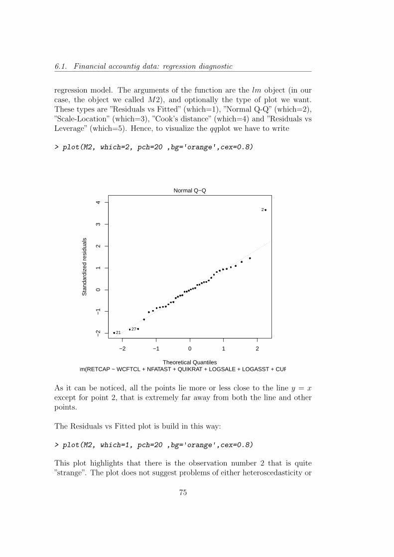
6.1. Financial accountig data: regression diagnostic
regression model. The arguments of the function are the lm object (in ourcase, the object we called M2), and optionally the type of plot we want.These types are ”Residuals vs Fitted” (which=1), ”Normal Q-Q” (which=2),”Scale-Location” (which=3), ”Cook’s distance” (which=4) and ”Residuals vsLeverage” (which=5). Hence, to visualize the qqplot we have to write
> plot(M2, which=2, pch=20 ,bg='orange',cex=0.8)
−2 −1 0 1 2
−2
−1
01
23
4
Theoretical Quantiles
Sta
ndar
dize
d re
sidu
als
lm(RETCAP ~ WCFTCL + NFATAST + QUIKRAT + LOGSALE + LOGASST + CURRAT)
Normal Q−Q
2
2127
As it can be noticed, all the points lie more or less close to the line y = xexcept for point 2, that is extremely far away from both the line and otherpoints.
The Residuals vs Fitted plot is build in this way:
> plot(M2, which=1, pch=20 ,bg='orange',cex=0.8)
This plot highlights that there is the observation number 2 that is quite”strange”. The plot does not suggest problems of either heteroscedasticity or
75

Linear regression: summary example 2
−0.2 0.0 0.2 0.4
−0.
10.
00.
10.
20.
3
Fitted values
Res
idua
ls
lm(RETCAP ~ WCFTCL + NFATAST + QUIKRAT + LOGSALE + LOGASST + CURRAT)
Residuals vs Fitted
2
20 27
non-linearity.
The package olsrr contains regression output, heteroscedasticity tests, collinear-ity diagnostics, residual diagnostics, measures of influence, model fit assess-ment and variable selection procedures. It allows to plot the studentizedresiduals vs fitted values. First, load the olsrr package
> install.packages("olsrr")
then, after it has been loaded
> require(olsrr)
use the function ols plot resid stud fit():
> ols_plot_resid_stud_fit(M2)
76

6.1. Financial accountig data: regression diagnostic
2
21
Threshold: abs(2)
−2
0
2
4
6
−0.25 0.00 0.25 0.50Predicted Value
Del
eted
Stu
dent
ized
Res
idua
l
Observation
normal
outlier
Deleted Studentized Residual vs Predicted Values
Look at the title of the figure. The term ”deleted studentized residuals”means ”externally studentized residuals” (or jackknife residuals). The plotalso places two bands to indicate the threshold value, that is equal to 2.
The same package produces the studentized residual plot, in which the (ex-ternally) studentized residuals are visualized with respect to the observations,highlighting the outliers:
> ols_plot_resid_stud(M2)
Given the threshold |ti| > 3, the observation number 2 is suggested as anoutlier.
77

Linear regression: summary example 2
2
Threshold: abs(3)
−2.5
0.0
2.5
5.0
0 10 20 30 40Observation
Delete
d Stud
entized
Residu
als
Observation
normal
outlier
Studentized Residuals Plot
6.1.2 Influencial points
The Cook’s distance and the measures of the DF family can be computed withthe function influence.measures(), with requires as input an object belong-ing to the lm class. This function returns information about the DFBETAof all the predictors, then the DFFITS, the covariance ratio, the Cook’sdistance and finally the leverage.
> M2infl <- influence.measures(M2)
> M2infl
Influence measures of
lm(formula = RETCAP ~ WCFTCL + NFATAST + QUIKRAT + LOGSALE + LOGASST + CURRAT, data = Jobson) :
dfb.1_ dfb.WCFT dfb.NFAT dfb.QUIK dfb.LOGS dfb.LOGA dfb.CURR dffit cov.r cook.d hat inf
1 -0.03864 0.123364 -0.093414 -0.413910 -2.69e-01 0.215319 0.351361 0.53177 1.2449 4.03e-02 0.2088
2 0.96542 0.656383 -1.313393 1.006111 8.33e-01 -0.909451 -1.066911 1.80826 0.0377 2.87e-01 0.1305 *
3 -0.01892 0.240180 0.672329 -0.040222 -4.19e-01 0.265794 -0.074710 0.99795 1.3965 1.40e-01 0.3758
4 0.05827 0.051934 -0.151360 0.140817 1.19e-01 -0.063276 -0.150290 0.31160 0.8212 1.34e-02 0.0431
5 -0.00687 -0.002145 -0.003119 -0.004719 -4.75e-06 0.005513 0.005152 0.01379 1.3143 2.80e-05 0.0569
6 0.01731 -0.001687 0.010656 -0.022026 -1.48e-02 -0.007568 0.021167 -0.04014 1.4808 2.37e-04 0.1639
7 0.02911 0.040491 -0.047395 0.049065 3.10e-02 -0.027750 -0.055437 0.07157 2.2765 7.55e-04 0.4559 *
8 0.02340 0.155241 0.053575 -0.138625 -6.67e-02 0.013835 0.104878 0.25471 1.1414 9.34e-03 0.0784
9 -0.00540 0.050331 0.137880 0.036227 -6.45e-02 0.033008 -0.063495 -0.26273 1.1933 9.97e-03 0.0964
10 -0.06588 -0.003786 0.055909 -0.332294 -9.31e-02 0.061339 0.335571 0.37489 1.4555 2.04e-02 0.2304
11 -0.08893 0.105491 0.085526 -0.092696 -7.23e-02 0.073371 0.076199 -0.24375 1.0785 8.50e-03 0.0598
12 -0.00800 -0.006016 -0.049558 -0.059821 -3.13e-02 0.033141 0.043305 -0.13967 1.4559 2.87e-03 0.1661
13 -0.01978 -0.765676 0.278492 0.298205 -4.17e-02 0.098246 -0.203557 0.90737 1.9457 1.18e-01 0.4758 *
14 0.06333 0.001086 0.035381 -0.013676 -3.82e-03 -0.045405 0.010299 0.09825 1.3051 1.42e-03 0.0743
15 -0.06441 -0.542879 -0.287285 0.130468 6.89e-02 0.061755 -0.047831 -0.74047 1.0642 7.62e-02 0.2231
16 -0.08276 -0.072517 0.021624 0.163870 -2.99e-01 0.198033 0.141360 2.46310 11.0767 8.76e-01 0.9028 *
17 0.02188 -0.024914 0.037266 -0.045335 -2.84e-02 -0.001218 0.045719 0.08886 1.2840 1.16e-03 0.0598
18 -0.00411 0.005277 -0.003384 0.006201 -5.66e-05 0.003686 -0.007417 -0.01744 1.2964 4.48e-05 0.0446
19 0.10444 0.038437 -0.045073 0.024637 4.16e-02 -0.092108 -0.028412 0.13391 1.3132 2.63e-03 0.0914
78

6.1. Financial accountig data: regression diagnostic
20 0.02468 0.338079 0.140440 0.002744 -7.03e-02 -0.023033 -0.054386 -0.52944 0.6548 3.73e-02 0.0751
21 -1.24497 -0.562435 1.410627 -0.025001 3.92e+00 -2.923101 1.063473 -5.03146 3.5355 3.29e+00 0.8548 *
22 -0.06327 0.083648 0.005653 -0.005665 -2.90e-02 0.054420 -0.008831 -0.17732 1.1422 4.55e-03 0.0489
23 0.07278 0.014416 -0.009756 0.019709 1.88e-03 -0.044753 -0.025507 0.07845 1.3870 9.05e-04 0.1149
24 -0.10683 0.065803 0.073481 -0.059875 -3.32e-02 0.065202 0.052782 -0.20552 1.1301 6.09e-03 0.0569
25 -0.03644 0.016082 0.001641 -0.037766 -3.32e-02 0.043083 0.032238 -0.06774 1.3165 6.75e-04 0.0703
26 0.02339 -0.393393 0.173081 0.175082 1.89e-01 -0.152252 -0.084678 0.51254 1.1685 3.73e-02 0.1796
27 -0.38459 -0.485481 -0.460930 0.073277 3.41e-03 0.359674 -0.003323 -0.90330 0.7243 1.08e-01 0.1854
28 0.01815 0.020758 0.024155 -0.019154 -6.18e-03 -0.025994 0.019620 -0.10580 1.2011 1.63e-03 0.0348
29 0.01603 0.020057 0.025953 0.040916 -1.37e-02 -0.003668 -0.045268 -0.09987 1.2899 1.46e-03 0.0671
30 -0.05731 0.040758 -0.054502 -0.004837 4.15e-02 0.022172 0.003845 0.14334 1.2434 3.00e-03 0.0648
31 -0.06266 0.044899 -0.083493 0.002556 -3.57e-02 0.084546 -0.021821 -0.16901 1.1998 4.15e-03 0.0608
32 -0.02791 0.052881 0.043869 -0.219959 -1.85e-01 0.107799 0.198940 -0.30931 1.0753 1.36e-02 0.0825
33 -0.13304 -0.010413 0.043305 -0.017949 -1.65e-02 0.103762 0.017748 0.16353 1.8173 3.93e-03 0.3257 *
34 0.00534 -0.000384 -0.023197 0.010527 -8.14e-03 0.005909 -0.012513 -0.05225 1.2717 4.01e-04 0.0389
35 0.01920 -0.000494 0.008321 -0.000626 -2.76e-03 -0.013850 0.000417 -0.02497 1.8375 9.19e-05 0.3252 *
36 -0.08888 -0.130096 0.215262 -0.235852 -2.01e-01 0.169343 0.231814 0.35084 1.1774 1.77e-02 0.1251
37 -0.02862 -0.007518 0.077961 0.048373 -4.31e-02 0.046391 -0.057911 -0.17512 1.2631 4.47e-03 0.0856
38 0.13700 -0.006820 0.057249 0.042112 -4.55e-02 -0.072767 -0.050934 -0.22186 1.1860 7.12e-03 0.0780
39 0.05227 0.045923 0.059127 -0.035519 -2.37e-02 -0.031911 0.025638 0.11071 1.3784 1.80e-03 0.1180
40 -0.00104 -0.000387 0.000935 -0.002591 3.82e-04 -0.000127 0.003031 0.00424 1.3333 2.65e-06 0.0697
The last column of the object M2infl contains an asterisk to highlight pointsthat we may consider as influential observations. Of course, a brief summaryis better than look at such a table (note that we have only 40 observationsand a few variables).
> summary(M2infl)
Potentially influential observations of
lm(formula = RETCAP ~ WCFTCL + NFATAST + QUIKRAT + LOGSALE + LOGASST + CURRAT, data = Jobson) :
dfb.1_ dfb.WCFT dfb.NFAT dfb.QUIK dfb.LOGS dfb.LOGA dfb.CURR dffit cov.r cook.d hat
2 0.97 0.66 -1.31_* 1.01_* 0.83 -0.91 -1.07_* 1.81_* 0.04_* 0.29 0.13
7 0.03 0.04 -0.05 0.05 0.03 -0.03 -0.06 0.07 2.28_* 0.00 0.46
13 -0.02 -0.77 0.28 0.30 -0.04 0.10 -0.20 0.91 1.95_* 0.12 0.48
16 -0.08 -0.07 0.02 0.16 -0.30 0.20 0.14 2.46_* 11.08_* 0.88 0.90_*
21 -1.24_* -0.56 1.41_* -0.03 3.92_* -2.92_* 1.06_* -5.03_* 3.54_* 3.29_* 0.85_*
33 -0.13 -0.01 0.04 -0.02 -0.02 0.10 0.02 0.16 1.82_* 0.00 0.33
35 0.02 0.00 0.01 0.00 0.00 -0.01 0.00 -0.02 1.84_* 0.00 0.33
By looking at the summary, it is clear that some observations are consideredas influential because for only one measure the threshold has been exceeded.For example, observation number 2 has only COV RATIO value larger thanthe threshold. On the other hand, observation 21 is considered influentialfor several measures: except for some DFBETA, it is indicated as potentialinfluence observation for all the measures. Visualizing through a plot theinfluential measures is even better. The following plot, made with the plot()function specifying which = 5, is mainly dedicated to the Cook’s distance.
> plot(M2, which=5, pch=20 ,bg='orange',cex=0.8)
79

Linear regression: summary example 2
0.0 0.2 0.4 0.6 0.8
−2
−1
01
23
4
Leverage
Sta
ndar
dize
d re
sidu
als
lm(RETCAP ~ WCFTCL + NFATAST + QUIKRAT + LOGSALE + LOGASST + CURRAT)
Cook's distance
10.5
0.51
Residuals vs Leverage
21
16
2
Patterns are not relevant for this plot. It is useful for detecting influentialobservations by looking at the upper right corner or at the lower right cor-ner. The dashed red line represents the Cook’s Distance, with levels set atDi = 0.5 and Di = 1. If cases are outside of the Cook’s distance (meaningthey have high Cook’s distance scores), the cases are influential to the regres-sion results. In this case, it is reported the case 21 as potential influentialobservation.
Also for the DF family is possible produce plots. The function ols plot dfbetas()of the package olsrr returns a plot for each coefficient, including the rule ofthumb |DF | = 2/sqrt(n) to detect potential influential observations. Herewe use the standard plot() function combined with functions dffits() anddfbetas(). We know that 2/
√n = 2/
√40 = 0.316 is the threshold for the
DFBETAs and 2×√
(p/n) = 2×√
6/40 = 0.0.775 is the threshold for theDFFITS, then graphically it is useful place two horizontal bands.
> #set the threshold for the DF family measures
80

6.1. Financial accountig data: regression diagnostic
> M2dff <- 2*sqrt(6/40)
> M2dfb <- 2/sqrt(40)
In order to do a subplot, we use the function par(), then we perform a loop-for. See Paradis (2010) for more details.
> #set the graphical window in order to accept 8 plots
> par(mfrow=c(2,4))
> plot(dffits(M2), pch=20, bg='orange', cex=0.8, ylab="DFFITS", main="DFFITS")
> #add threshold lines for DF fits
> abline(h=M2dff, lty=2, col=2)
> abline(h=-M2dff, lty=2, col=2)
> #extract the name of the variables from M2 object
> CN=colnames(dfbeta(M2))
> #Do plots for the intercept + 6 predictors
> for(j in 1:7)
+ plot(dfbetas(M2)[,j], pch=20, bg='orange', cex=0.8, ylab="DFBETA",main=CN[j])
+ #add treshold linesfor DF beta
+ abline(h=M2dfb, lty=2, col=2)
+ abline(h=-M2dfb, lty=2, col=2)
+
0 10 20 30 40
−4
−2
02
DFFITS
Index
DF
FIT
S
0 10 20 30 40
−1.
0−
0.5
0.0
0.5
1.0
(Intercept)
Index
DF
BE
TA
0 10 20 30 40
−0.
8−
0.4
0.0
0.4
WCFTCL
Index
DF
BE
TA
0 10 20 30 40
−1.
00.
00.
51.
01.
5
NFATAST
Index
DF
BE
TA
0 10 20 30 40
−0.
40.
00.
40.
8
QUIKRAT
Index
DF
BE
TA
0 10 20 30 40
01
23
4
LOGSALE
Index
DF
BE
TA
0 10 20 30 40
−3.
0−
2.0
−1.
00.
0
LOGASST
Index
DF
BE
TA
0 10 20 30 40
−1.
0−
0.5
0.0
0.5
1.0
CURRAT
Index
DF
BE
TA
Here we computed ”by hand”all the threshold. By using the function ols plot dfbetas()of the package olsrr we obtain
81

Linear regression: summary example 2
> ols_plot_dfbetas(M2)
2
21
27
Threshold: 0.32
−1.0
−0.5
0.0
0.5
1.0
0 10 20 30 40Observation
DFB
ETAS
Influence Diagnostics for (Intercept)
2
13
15
20
21
26
27
Threshold: 0.32
−0.8
−0.4
0.0
0.4
0 10 20 30 40Observation
DFB
ETAS
Influence Diagnostics for WCFTCL
2
3
21
27
Threshold: 0.32
−1.0
−0.5
0.0
0.5
1.0
1.5
0 10 20 30 40Observation
DFB
ETAS
Influence Diagnostics for NFATAST
1
2
10
Threshold: 0.32
0.0
0.5
1.0
0 10 20 30 40Observation
DFB
ETAS
Influence Diagnostics for QUIKRAT
page 1 of 2
2
3
21 Threshold: 0.32
0
1
2
3
4
0 10 20 30 40Observation
DFB
ETAS
Influence Diagnostics for LOGSALE
2
21
27Threshold: 0.32
−3
−2
−1
0
0 10 20 30 40Observation
DFB
ETAS
Influence Diagnostics for LOGASST
1
2
10
21 Threshold: 0.32
−1.0
−0.5
0.0
0.5
1.0
0 10 20 30 40Observation
DFB
ETAS
Influence Diagnostics for CURRATpage 2 of 2
In these plots there are the same information visualized before. Being dedi-cated plots, probably they are more clear.
82

6.1. Financial accountig data: regression diagnostic
Finally, a plot representing the Hadi’s H2 measure is possible through thefunction ols plot hadi().
> ols_plot_hadi(M2)
0.0
2.5
5.0
7.5
0 10 20 30 40Observation
Hadi
's M
easu
re
Hadi's Influence Measure
The highest Hadi’s value is associated to the observation number 16
6.1.3 Collinearity detection
There are several R packages dedicated to multicollinearity diagnostic mea-sures. The package mctest is dedicated to the computation of popular andwidely used multicollinearity diagnostic measures. Let’s install the package
> install.packages("mctest")
then load it:
> require(mctest)
The function eigprop() computes eigenvalues, condition indices and variancedecomposition proportions of XTX.The collinearity diagnostics for the financial accounting data are:
83
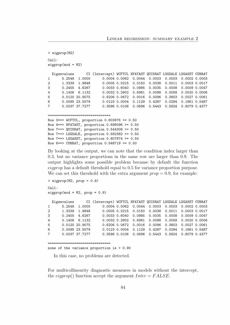
Linear regression: summary example 2
> eigprop(M2)
Call:
eigprop(mod = M2)
Eigenvalues CI (Intercept) WCFTCL NFATAST QUIKRAT LOGSALE LOGASST CURRAT
1 5.2548 1.0000 0.0004 0.0062 0.0044 0.0003 0.0003 0.0002 0.0003
2 1.3339 1.9848 0.0005 0.0215 0.0150 0.0038 0.0011 0.0003 0.0017
3 0.2455 4.6267 0.0033 0.6040 0.0985 0.0035 0.0008 0.0009 0.0047
4 0.1406 6.1132 0.0032 0.2902 0.6981 0.0098 0.0058 0.0020 0.0006
5 0.0120 20.9075 0.6206 0.0672 0.0016 0.0096 0.3803 0.0027 0.0061
6 0.0095 23.5579 0.0123 0.0004 0.1129 0.4287 0.0294 0.1861 0.5487
7 0.0037 37.7277 0.3596 0.0106 0.0696 0.5443 0.5824 0.8079 0.4377
===============================
Row 3==> WCFTCL, proportion 0.603976 >= 0.50
Row 4==> NFATAST, proportion 0.698096 >= 0.50
Row 7==> QUIKRAT, proportion 0.544308 >= 0.50
Row 7==> LOGSALE, proportion 0.582382 >= 0.50
Row 7==> LOGASST, proportion 0.807874 >= 0.50
Row 6==> CURRAT, proportion 0.548719 >= 0.50
By looking at the output, we can note that the condition index larger than0.3, but no variance proportions in the same row are larger than 0.9. Theoutput highlights some possible problem because by default the functioneigprop has a default threshold equal to 0.5 for variance proportion purpose.We can set this threshold with the extra argument prop = 0.9, for example:
> eigprop(M2, prop = 0.9)
Call:
eigprop(mod = M2, prop = 0.9)
Eigenvalues CI (Intercept) WCFTCL NFATAST QUIKRAT LOGSALE LOGASST CURRAT
1 5.2548 1.0000 0.0004 0.0062 0.0044 0.0003 0.0003 0.0002 0.0003
2 1.3339 1.9848 0.0005 0.0215 0.0150 0.0038 0.0011 0.0003 0.0017
3 0.2455 4.6267 0.0033 0.6040 0.0985 0.0035 0.0008 0.0009 0.0047
4 0.1406 6.1132 0.0032 0.2902 0.6981 0.0098 0.0058 0.0020 0.0006
5 0.0120 20.9075 0.6206 0.0672 0.0016 0.0096 0.3803 0.0027 0.0061
6 0.0095 23.5579 0.0123 0.0004 0.1129 0.4287 0.0294 0.1861 0.5487
7 0.0037 37.7277 0.3596 0.0106 0.0696 0.5443 0.5824 0.8079 0.4377
===============================
none of the variance proportion is > 0.90
In this case, no problems are detected.
For multicollinearity diagnostic measures in models without the intercept,the eigprop() function accept the argument Inter = FALSE.
84

6.1. Financial accountig data: regression diagnostic
> eigprop(M2, Inter = FALSE)
Call:
eigprop(mod = M2, Inter = FALSE)
Eigenvalues CI WCFTCL NFATAST QUIKRAT LOGSALE LOGASST CURRAT
1 4.3810 1.0000 0.0104 0.0060 0.0005 0.0004 0.0005 0.0006
2 1.2436 1.8769 0.0167 0.0253 0.0040 0.0016 0.0009 0.0017
3 0.2274 4.3896 0.7735 0.0446 0.0051 0.0019 0.0028 0.0071
4 0.1336 5.7262 0.1945 0.7568 0.0093 0.0119 0.0076 0.0001
5 0.0095 21.4623 0.0003 0.1079 0.4212 0.0747 0.3055 0.6264
6 0.0049 29.8489 0.0046 0.0593 0.5599 0.9094 0.6828 0.3641
===============================
Row 3==> WCFTCL, proportion 0.773508 >= 0.50
Row 4==> NFATAST, proportion 0.756804 >= 0.50
Row 6==> QUIKRAT, proportion 0.559943 >= 0.50
Row 6==> LOGSALE, proportion 0.909363 >= 0.50
Row 6==> LOGASST, proportion 0.682771 >= 0.50
Row 5==> CURRAT, proportion 0.626402 >= 0.50
85


Chapter 7
Remedies for assumptionviolations andMulticollinearity: a shortoverview
7.1 Introduction
In this chapter a brief overview of possible remedies to violation of classicalhypotheses in a regression model is introduced. Students will study bothmany of the proposed solutions in more details and new approaches in otherexams (Econometric, Statistical learning, etc.).
7.2 Outliers
If outliers have been detected, most of the time they are due to a data entryerror: in this case just correct the value. If outliers are due to invalid cases,these cases may be eliminated. In any case, report the number of cases ex-cluded and the reason. Better, analyze the data and/or reporting analyseswith and without the deleted cases.
Look at the data: are the data expressed in too different scale of measure-ment? Transformation of the data might be considered (square root, loga-rithm, Box-Cox transformation). However, sometimes transformations canmake results difficult to interpret.
Data should be analyzed with and without the outliers. If the results do not

Remedies for assumption violations and Multicollinearity
differ (better, if the implications of the results do not differ), then one couldsimply state that the analyses were conducted with and without the outliersand that the results do not differ substantially. If they do differ, a discussionabout the potential causes of the outlier(s) could be discussed (e.g., differentsubgroup of cases, potential moderator effect).Alternative estimation method could be used (robust regression; Least abso-lute regression; when there are are clusters of outliers multilevel models orlinear mixed-effect models; and so on)
7.3 Not independent errors and hetersoscedas-
ticity
The standard assumption about the error term ε is that it is independent andidentically distributed (i.i.d.) from case to case. That is, var[ε] = E[εεT ] =σ2I. When the errors are not i.i.d., the use of Generalized Least Squares(GLS) can solve the problem.
7.3.1 GLS
Sometimes the errors have non-constant variance or are correlated. Classicalexamples are time-dependent data. Suppose that var[ε] = E[εεT ] = σ2Ω. IfΩ 6= I, the OLS estimator B = (XTX−1)XTY has covariance matrix equalto σ2(XTX)−1(XTΩX)(XTX)−1, hence it is no longer the minimum varianceunbiased estimator (recall that the Gauss-Markov theorem states that OLSestimator is BLUE under the classical hypotheses). Suppose that Ω existsand it is known, then the GLS estimator
BGLS = (XTΩ−1X)−1XTΩ−1Y
has E[BGLS ] = β and covariance matrix σ2(XTΩ−1X)−1 and is the bestlinear unbiased estimator for β because is equivalent to applying ordinaryleast squares to a linearly transformed version of the data. Suppose indeedthat Ω−1 = PTP, and define X∗ = PX, Y∗ = PY and ε∗ = Pε, then
BGLS = (X∗TX∗)−1X∗TY∗,
with covariance matrix σ2(X∗TX∗)−1 = σ2(XTΩ−1X)−1. The data transfor-mation theoretically has the effect of standardizing the scale of the errorsand ”de-correlating” them. Then OLS is applied to data with homoscedasticerrors and, as the Gauss-Markov theorem applies, the GLS estimate is the
88
7.4. Collinearity remedies
best linear unbiased estimator for β.
In practical cases neither σ2 nor Ω are known. We already know how toestimate σ2. We need some information about the structure of Ω, that cannotbe estimated from the sample data.
7.3.2 WLS
The errors may be independent, but not identically distributed. In this caseΩ is a diagonal matrix (i.e., it has zero on the extradiagonal elements) withnon constant values, hence revealing hetersoscedasticity. In such a case, theWeighted Least Squares (WLS) model can be used, which is a special case ofGLS. The weight for the ith unit is proportional to the reciprocal of the vari-ance of the response for unit i. By writing Ω = diag(1/ω1, 1/ω2, . . . , 1/ωn),where ωi represents the ith weight, cases with low variability should get ahigh weight, high variability a low weight.
7.4 Collinearity remedies
Multicollinearity can sometimes be caused by artificially restricting the sam-ple in some way, but it can also be natural to the population and can onlybe eliminated by model respecification. When multicollinearity is present, ifpossible adding new data is often the best way of reducing its effects. Some-times it may be possible to eliminate variables on a theoretical basis thatwould also reduce collinearity.
7.4.1 Ridge regression
Multicollinearity can increase the variance of the least squares estimator.So, the problem of a near-singular moment matrix (XTX) is alleviated byadding positive elements to its diagonals elements. Of course, in this waythe requirement that the estimator be unbiased is removed, but we gain invariance reduction (you will study the Bias-Variance Dilemma soon). Let kbe a positive constant, the Ridge regression objective function is
f(β) = (y −Xβ)T (y −Xβ) + k(βTβ) = min,
whose minimizer isβR =
[XTX + kI
]−1XTy.
The Ridge parameter k serves as the positive constant shifting the diagonalsdecreasing the condition number of the moment matrix. Ridge regression
89

Remedies for assumption violations and Multicollinearity
belongs to the family of shrinked regressions (probably you will study theLASSO regression, the elastic net regression, etc.)
The ridge regression estimator is biased, indeed
E[BR] = β − k(XTX + kI
)−1β.
The variance of the Ridge estimator is equal to
var(BR) =(XTX + kI
)−1σ2XTX
(XTX + kI
)−1.
As k increases the variance term decreases and the bias term increases. Thereare many ways to determine the ”right” k parameter (cross-validation, gen-eralized cross-validation, L-curve,...). One of them is to choose k in such away that the decrease in the variance due to k is larger than the increase inbias.
7.5 Principal Component Regression
A possible solution to correlated predictors is to orthogonalize them priorto proceed to the regression analysis. In Chapter 5.5.1 we introduced theeigenvalues and the eigenvectors of a square matrix. Let Λ and V thediagonal matrix of the eigenvalues and the matrix of the eigenvectors ofXTX. The matrix Z = XV has the columns orthogonal to each other, andZTZ = VTXTXV = Λ. It means that λ1, λ2, . . . , λp are the variances of Z.The columns of Z are called principal components, the variance of zi is λi.Ideally, only a few eigenvalues will be large so that almost all the variationin X will be representable by those first few principal component. Keep inmind that (all) the principal components are linear combination of (all) thepredictors: it may be the case that many of these components are not inter-pretable at all. Principal components do not use the response variables: itmay be the case that a lesser principal component is actually very importantin predicting the response.If the measurement scale of the predictors is unbalanced, often Z = XV,where X contains standardized columns (centered and scaled to be vari-ance=1) and V contains the eigenvectors of the correlation matrix R.
7.6 Practical examples
This chapter is dedicated to some practical examples
90
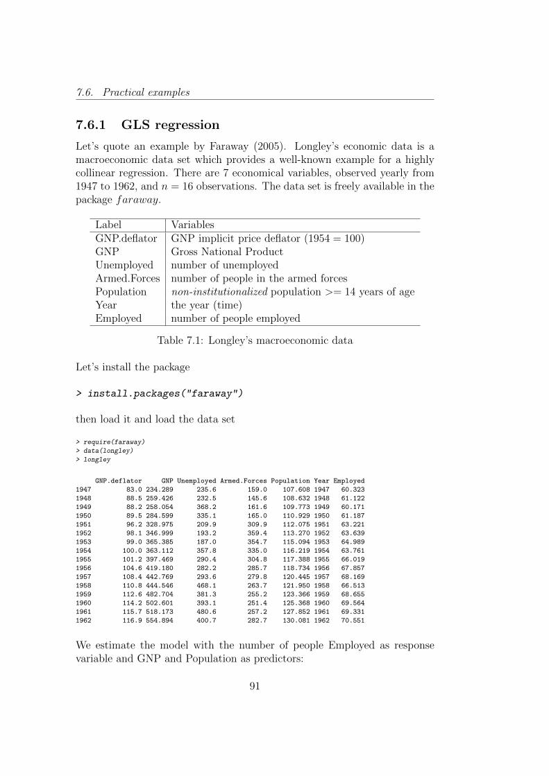
7.6. Practical examples
7.6.1 GLS regression
Let’s quote an example by Faraway (2005). Longley’s economic data is amacroeconomic data set which provides a well-known example for a highlycollinear regression. There are 7 economical variables, observed yearly from1947 to 1962, and n = 16 observations. The data set is freely available in thepackage faraway.
Label VariablesGNP.deflator GNP implicit price deflator (1954 = 100)GNP Gross National ProductUnemployed number of unemployedArmed.Forces number of people in the armed forcesPopulation non-institutionalized population >= 14 years of ageYear the year (time)Employed number of people employed
Table 7.1: Longley’s macroeconomic data
Let’s install the package
> install.packages("faraway")
then load it and load the data set
> require(faraway)
> data(longley)
> longley
GNP.deflator GNP Unemployed Armed.Forces Population Year Employed
1947 83.0 234.289 235.6 159.0 107.608 1947 60.323
1948 88.5 259.426 232.5 145.6 108.632 1948 61.122
1949 88.2 258.054 368.2 161.6 109.773 1949 60.171
1950 89.5 284.599 335.1 165.0 110.929 1950 61.187
1951 96.2 328.975 209.9 309.9 112.075 1951 63.221
1952 98.1 346.999 193.2 359.4 113.270 1952 63.639
1953 99.0 365.385 187.0 354.7 115.094 1953 64.989
1954 100.0 363.112 357.8 335.0 116.219 1954 63.761
1955 101.2 397.469 290.4 304.8 117.388 1955 66.019
1956 104.6 419.180 282.2 285.7 118.734 1956 67.857
1957 108.4 442.769 293.6 279.8 120.445 1957 68.169
1958 110.8 444.546 468.1 263.7 121.950 1958 66.513
1959 112.6 482.704 381.3 255.2 123.366 1959 68.655
1960 114.2 502.601 393.1 251.4 125.368 1960 69.564
1961 115.7 518.173 480.6 257.2 127.852 1961 69.331
1962 116.9 554.894 400.7 282.7 130.081 1962 70.551
We estimate the model with the number of people Employed as responsevariable and GNP and Population as predictors:
91

Remedies for assumption violations and Multicollinearity
> Mlong1 <- lm(Employed ~ GNP + Population, data = longley)
> summary(Mlong1)
Call:
lm(formula = Employed ~ GNP + Population, data = longley)
Residuals:
Min 1Q Median 3Q Max
-0.80899 -0.33282 -0.02329 0.25895 1.08800
Coefficients:
Estimate Std. Error t value Pr(>|t|)
(Intercept) 88.93880 13.78503 6.452 2.16e-05 ***
GNP 0.06317 0.01065 5.933 4.96e-05 ***
Population -0.40974 0.15214 -2.693 0.0184 *
---
Signif. codes: 0 '***' 0.001 '**' 0.01 '*' 0.05 '.' 0.1 ' ' 1
Residual standard error: 0.5459 on 13 degrees of freedom
Multiple R-squared: 0.9791, Adjusted R-squared: 0.9758
F-statistic: 303.9 on 2 and 13 DF, p-value: 1.221e-11
Let’s give a look to the residuals versus fitted plot:
> plot(Mlong1, which=1)
60 62 64 66 68 70
−1.
0−
0.5
0.0
0.5
1.0
Fitted values
Res
idua
ls
lm(Employed ~ GNP + Population)
Residuals vs Fitted
1956
1952
1947
It is clear that the residuals do not have a random pattern close to the zerohorizontal line. Probably they are correlated. Of course we do not knowΩ. But we can imagine that error follow a simple autoregressive function
92

7.6. Practical examples
(namely εi+1 = φεi + γi, in which γi has zero mean and constant variance).The package nlme contains the function gls(), that allows to estimate GLSregression.
> install.packages("nlme")
> require(nlme)
> MlongGLS <- gls(Employed ~ GNP + Population, correlation = corAR1(),
+ data = longley)
> summary(MlongGLS)
Generalized least squares fit by REML
Model: Employed ~ GNP + Population
Data: longley
AIC BIC logLik
44.66377 47.48852 -17.33188
Correlation Structure: AR(1)
Formula: ~1
Parameter estimate(s):
Phi
0.6441692
Coefficients:
Value Std.Error t-value p-value
(Intercept) 101.85813 14.198932 7.173647 0.0000
GNP 0.07207 0.010606 6.795485 0.0000
Population -0.54851 0.154130 -3.558778 0.0035
Correlation:
(Intr) GNP
GNP 0.943
Population -0.997 -0.966
Standardized residuals:
Min Q1 Med Q3 Max
-1.5924564 -0.5447822 -0.1055401 0.3639202 1.3281898
Residual standard error: 0.689207
Degrees of freedom: 16 total; 13 residual
Look at the summary of the model. The parameter called ”Phi” is the first-order correlation among the error terms. It is equal to 0.6442, but it is
93

Remedies for assumption violations and Multicollinearity
statistically not different from zero. By using the function intervals(), whichis a function that computes confidence intervals on the parameters associatedwith the model represented by the input, we can see that the confidenceinterval for the (auto)correlation coefficient contains zero, hence there is noevidence of serial correlation.
> intervals(MlongGLS)
Approximate 95% confidence intervals
Coefficients:
lower est. upper
(Intercept) 71.18320460 101.85813305 132.5330615
GNP 0.04915865 0.07207088 0.0949831
Population -0.88149053 -0.54851350 -0.2155365
attr(,"label")
[1] "Coefficients:"
Correlation structure:
lower est. upper
Phi -0.4432383 0.6441692 0.9645041
attr(,"label")
[1] "Correlation structure:"
Residual standard error:
lower est. upper
0.2477527 0.6892070 1.9172599
7.6.2 WLS regression
Let’s quote an example by Faraway (2002). From the faraway package loadthe data set strongx
> data(strongx)
> strongx
momentum energy crossx sd
1 4 0.345 367 17
2 6 0.287 311 9
3 8 0.251 295 9
4 10 0.225 268 7
5 12 0.207 253 7
6 15 0.186 239 6
94
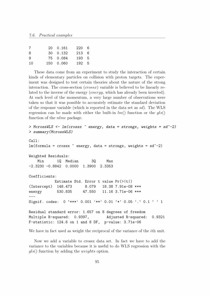
7.6. Practical examples
7 20 0.161 220 6
8 30 0.132 213 6
9 75 0.084 193 5
10 150 0.060 192 5
These data come from an experiment to study the interaction of certainkinds of elementary particles on collision with proton targets. The exper-iment was designed to test certain theories about the nature of the stronginteraction. The cross-section (crossx) variable is believed to be linearly re-lated to the inverse of the energy (energy, which has already been inverted).At each level of the momentum, a very large number of observations weretaken so that it was possible to accurately estimate the standard deviationof the response variable (which is reported in the data set as sd). The WLSregression can be made with either the built-in lm() function or the gls()function of the nlme package.
> McrossWLS <- lm(crossx ~ energy, data = strongx, weights = sd^-2)
> summary(McrossWLS)
Call:
lm(formula = crossx ~ energy, data = strongx, weights = sd^-2)
Weighted Residuals:
Min 1Q Median 3Q Max
-2.3230 -0.8842 0.0000 1.3900 2.3353
Coefficients:
Estimate Std. Error t value Pr(>|t|)
(Intercept) 148.473 8.079 18.38 7.91e-08 ***
energy 530.835 47.550 11.16 3.71e-06 ***
---
Signif. codes: 0 '***' 0.001 '**' 0.01 '*' 0.05 '.' 0.1 ' ' 1
Residual standard error: 1.657 on 8 degrees of freedom
Multiple R-squared: 0.9397, Adjusted R-squared: 0.9321
F-statistic: 124.6 on 1 and 8 DF, p-value: 3.71e-06
We have in fact used as weight the reciprocal of the variance of the ith unit.
Now we add a variable to crossx data set. In fact we have to add thevariance to the variables because it is useful to do WLS regression with thegls() function by adding the weights option.
95

Remedies for assumption violations and Multicollinearity
> strongx$sd2 <- strongx$sd^2
> strongx
momentum energy crossx sd sd2
1 4 0.345 367 17 289
2 6 0.287 311 9 81
3 8 0.251 295 9 81
4 10 0.225 268 7 49
5 12 0.207 253 7 49
6 15 0.186 239 6 36
7 20 0.161 220 6 36
8 30 0.132 213 6 36
9 75 0.084 193 5 25
10 150 0.060 192 5 25
In the commands we must specify that the variance is fixed (the argumentvarF ixed), in the sense that it must not be re-estimated during the itera-tions. The sd2 variable is the variance we added to the data set. Finally,method = ”ML” means that we use the Maximum Likelihood estimate ofthe parameters.
> McrossWLS2 <- gls(crossx ~ energy, data = strongx, weights = varFixed(~sd2),
+ method = "ML")
> summary(McrossWLS2)
Generalized least squares fit by maximum likelihood
Model: crossx ~ energy
Data: strongx
AIC BIC logLik
81.66907 82.57683 -37.83454
Variance function:
Structure: fixed weights
Formula: ~sd2
Coefficients:
Value Std.Error t-value p-value
(Intercept) 148.4732 8.07865 18.37847 0
energy 530.8354 47.55003 11.16372 0
Correlation:
96
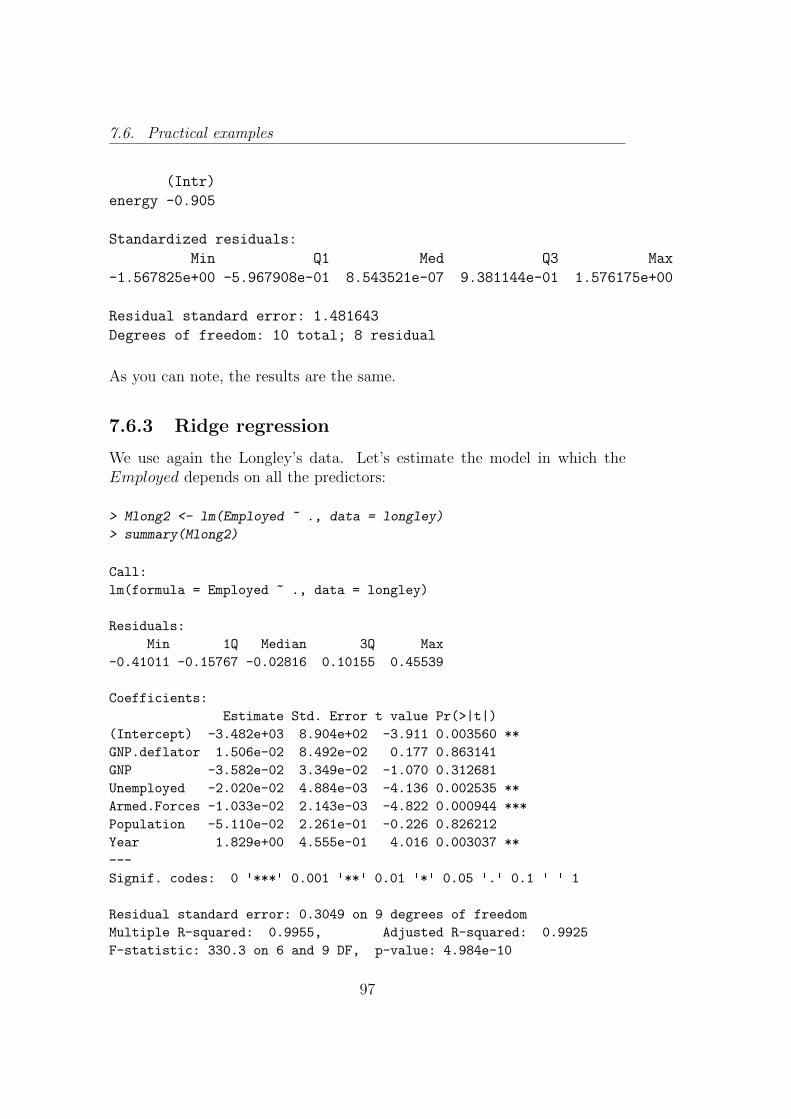
7.6. Practical examples
(Intr)
energy -0.905
Standardized residuals:
Min Q1 Med Q3 Max
-1.567825e+00 -5.967908e-01 8.543521e-07 9.381144e-01 1.576175e+00
Residual standard error: 1.481643
Degrees of freedom: 10 total; 8 residual
As you can note, the results are the same.
7.6.3 Ridge regression
We use again the Longley’s data. Let’s estimate the model in which theEmployed depends on all the predictors:
> Mlong2 <- lm(Employed ~ ., data = longley)
> summary(Mlong2)
Call:
lm(formula = Employed ~ ., data = longley)
Residuals:
Min 1Q Median 3Q Max
-0.41011 -0.15767 -0.02816 0.10155 0.45539
Coefficients:
Estimate Std. Error t value Pr(>|t|)
(Intercept) -3.482e+03 8.904e+02 -3.911 0.003560 **
GNP.deflator 1.506e-02 8.492e-02 0.177 0.863141
GNP -3.582e-02 3.349e-02 -1.070 0.312681
Unemployed -2.020e-02 4.884e-03 -4.136 0.002535 **
Armed.Forces -1.033e-02 2.143e-03 -4.822 0.000944 ***
Population -5.110e-02 2.261e-01 -0.226 0.826212
Year 1.829e+00 4.555e-01 4.016 0.003037 **
---
Signif. codes: 0 '***' 0.001 '**' 0.01 '*' 0.05 '.' 0.1 ' ' 1
Residual standard error: 0.3049 on 9 degrees of freedom
Multiple R-squared: 0.9955, Adjusted R-squared: 0.9925
F-statistic: 330.3 on 6 and 9 DF, p-value: 4.984e-10
97

Remedies for assumption violations and Multicollinearity
Look at the results: except for the intercept, only three predictors are statis-tically significant. On the other hand, both R2 and R
′2 are higher than 0.9,suggesting excellent fit. Probably there are collinearity problems. Let’s givea look to the VIF and the tolerance. We use the function imcdiag() from thepackage mctest.
> Vifslong <- imcdiag(Mlong2)
> Vifslong$idiags[, 1:2]
VIF TOL
GNP.deflator 135.53244 0.0073783075
GNP 1788.51348 0.0005591235
Unemployed 33.61889 0.0297451814
Armed.Forces 3.58893 0.2786345641
Population 399.15102 0.0025053174
Year 758.98060 0.0013175567
The VIF for 5 variables are larger than the threshold value of 10. The packagemctest contains a graphical tool that allows to plot both VIF and Eigenvaluesfor detection of multicollinearity among regressors.
> mc.plot(Mlong2, Inter=TRUE)
050
010
00
VIF Plot
VIF
val
ues
GNP.deflator GNP Unemployed Armed.Forces Population Year
135.532
1788.513
33.619 3.589
399.151
758.981
VIF threshold = 10
01
23
45
67
Eigenvalues Plot
Eig
enva
lues
EV 1 EV 2 EV 3 EV 4 EV 5 EV 6 EV 7
6.861
0.082 0.046 0.011 0 0 0
EV threshold = 0.01
98

7.6. Practical examples
The upper panel of the figure highlights with a dashed red horizontal line thethreshold. It is clear that at least three predictors have a VIF much largerthan 10.The bottom panel shows that the first eigenvalue greatly dominates the otherones.
99

Remedies for assumption violations and Multicollinearity
Let’s examine the variance proportion and the condition index too:
> eigprop(Mlong2)
Call:
eigprop(mod = Mlong2)
Eigenvalues CI (Intercept) GNP.deflator GNP Unemployed
1 6.8614 1.0000 0.0000 0.0000 0.0000 0.0000
2 0.0821 9.1417 0.0000 0.0000 0.0000 0.0143
3 0.0457 12.2557 0.0000 0.0000 0.0003 0.0008
4 0.0107 25.3366 0.0000 0.0003 0.0011 0.0646
5 0.0001 230.4239 0.0000 0.4568 0.0157 0.0056
6 0.0000 1048.0803 0.0001 0.5046 0.3284 0.2253
7 0.0000 43275.0423 0.9999 0.0383 0.6546 0.6893
Armed.Forces Population Year
1 0.0004 0.0000 0.0000
2 0.0919 0.0000 0.0000
3 0.0636 0.0000 0.0000
4 0.4267 0.0000 0.0000
5 0.1154 0.0097 0.0000
6 0.0000 0.8306 0.0002
7 0.3020 0.1597 0.9998
===============================
Row 6==> GNP.deflator, proportion 0.504556 >= 0.50
Row 7==> GNP, proportion 0.654628 >= 0.50
Row 7==> Unemployed, proportion 0.689257 >= 0.50
Row 6==> Population, proportion 0.830564 >= 0.50
Row 7==> Year, proportion 0.999839 >= 0.50
This summary shows that the intercept, Y ear and (a bit less) UnemployedandGNP are strongly related to the smallest eigenvalue. The second smallesteigenvalue contributes a large proportion of the variance in the coefficient ofPopulation.We can examine the same information excluding the intercept
100

7.6. Practical examples
> eigprop(Mlong2, Inter = FALSE)
Call:
eigprop(mod = Mlong2, Inter = FALSE)
Eigenvalues CI GNP.deflator GNP Unemployed Armed.Forces Population
1 5.8734 1.0000 0.0000 0.0000 0.0002 0.0007 0.0000
2 0.0814 8.4928 0.0000 0.0000 0.0455 0.1469 0.0000
3 0.0343 13.0763 0.0000 0.0011 0.0036 0.0684 0.0000
4 0.0107 23.4773 0.0004 0.0030 0.2168 0.6200 0.0000
5 0.0001 214.7467 0.4640 0.0413 0.0154 0.1639 0.0146
6 0.0000 1086.0170 0.5355 0.9546 0.7185 0.0000 0.9854
Year
1 0.0000
2 0.0000
3 0.0001
4 0.0000
5 0.0021
6 0.9978
===============================
Row 6==> GNP.deflator, proportion 0.535530 >= 0.50
Row 6==> GNP, proportion 0.954569 >= 0.50
Row 6==> Unemployed, proportion 0.718462 >= 0.50
Row 4==> Armed.Forces, proportion 0.620011 >= 0.50
Row 6==> Population, proportion 0.985367 >= 0.50
Row 6==> Year, proportion 0.997767 >= 0.50
The smallest eigenvalue in this case contributes a large proportion of thevariance in the estimate of the coefficients of Y ear, Population, GNP andUnemployed. The results are really similar. We can proceed with the Ridgeregression. First, let’s install the lmridge package, that fits a linear ridgeregression model.
> install.packages("lmridge")
> require(lmridge)
> Mlongridge <- lmridge(Employed ~ ., data = longley, scaling = "scaled",
+ K = seq(from = 0, to = 0.01, length = 100))
We have set scaling = scaled to standardize the predictors to have zero meanand unit variance and a sequence of values from = 0 (OLS estimation) to0.01 as values of k. A grid of values of k, usually between 0 and 1, are tried.
101

Remedies for assumption violations and Multicollinearity
> Mlongridge
GNP.deflator GNP Unemployed Armed.Forces Population Year
K=0 0.162540999070495 -3.56024509766538 -1.8878325226559 -0.719042832692358 -0.355485349133805 8.70850284633467
K=0.000101010101010101 0.15135794060728 -3.46257991313349 -1.87449794831016 -0.716406583740208 -0.384598197698927 8.64125108620702
K=0.000202020202020202 0.140716844196331 -3.36835696682724 -1.86161774199345 -0.713848274534704 -0.412442688222477 8.57596447487405
K=0.000303030303030303 0.130588890760085 -3.2774005069751 -1.84916881115094 -0.711364027735968 -0.439085394832075 8.51254573951848
K=0.000404040404040404 0.120947197102774 -3.18954651572696 -1.83712960389496 -0.708950223832329 -0.464588428344471 8.45090407030022
.. .. .. .. .. .. ..
K=0.0095959595959596 -0.0246588333130088 -0.158052569465026 -1.40129782752144 -0.606095934146693 -1.03518087234433 5.80754726356318
K=0.0096969696969697 -0.0235729045243546 -0.14570423902045 -1.39933281301157 -0.605495245257635 -1.03470092471034 5.79211103740903
K=0.0097979797979798 -0.0224715947150985 -0.133531190496458 -1.39739206996953 -0.604899618481748 -1.03417578833667 5.77680755723676
K=0.0098989898989899 -0.0213553964199283 -0.121529922113921 -1.39547513075078 -0.604308969361412 -1.03360666119341 5.76163466771411
K=0.01 -0.0202247878428959 -0.109697023212352 -1.39358153973942 -0.603723215502928 -1.03299470769398 5.74659026556203
By typing Mlongridge, all the coefficients for all the values of k are displayed.Which model we must choose? There are several way to proceed. Here weuse the method of the minimum Mean Squared Error (MSE). Remember thatthe variance of a estimator is only one part of the MSE. When an estimatoris unbiased, then MSE=variance, but if it is biased, MSE=variance+squareof bias. The function rstast1() computes the ordinary ridge related statisticssuch as variance, squared bias, MSE, R-squared, etc.
> statlongridge <- rstats1(Mlongridge)
var bias2 mse
K=0 17.39421 0.00000000 17.39421
K=0.000101010101010101 16.86844 0.01521867 16.88366
K=0.000202020202020202 16.37155 0.05882211 16.43037
K=0.000303030303030303 15.90150 0.12796400 16.02946
K=0.000404040404040404 15.45619 0.22008074 15.67627
From the object statlongridge here squared bias, variance and MSE arehighlighted for the first five values of k. Note that as k increases, the squaredbias increases and the variance decreases. The sum of these two quantitiesgives the MSE, which is decreasing for these values of k.
102

7.6. Practical examples
0.000 0.002 0.004 0.006 0.008 0.010
05
1015
2025
Bias, Variance Tradeoff
Biasing Parameter
Var
Bias^2
MSE
min MSE 13.982 at K= 0.00161616161616162
Look at the figure: When k = 0, MSE=Variance because the squared biasequals zero (when k = 0 ridge regression and OLS regression are the samemodel). When k increases the squared bias increases (Ridge estimator isbiased) and the variance decreases (remember the effect of k on the diagonalelements of XTX. There is a range of k for which the MSE of ridge regressionis smaller than the MSE of OLS regression. The optimal k could be selectedwithin this range. The final model is then the one with the minimum MSE:
> #extract the index of the minimum MSE
> optkridge <- which.min(statlongridge$mse)
> #then find the k values
> minK=Mlongridge$K[optkridge]
> #finally visualize the model
> Mlongridgebest <- lmridge(Employed~., data=longley, scaling="scaled", K=minK)
> Mlongridgebest
103

Remedies for assumption violations and Multicollinearity
Call:
lmridge.default(formula = Employed ~ ., data = longley, K = minK,
scaling = "scaled")
Intercept GNP.deflator GNP Unemployed Armed.Forces Population Year
-3117.49153 0.00328 -0.02344 -0.01839 -0.00983 -0.10057 1.64329
The covariance matrix can be extracted with the function vcov():
> vcov(Mlongridgebest)
$`K=0.00161616161616162`
GNP.deflator GNP Unemployed Armed.Forces Population Year
GNP.deflator 0.63432595 -1.1417402 -0.12619166 -0.030186159 0.586812167 0.02127266
GNP -1.14174020 6.1327059 0.78934017 0.125574931 -2.452950249 -3.11307226
Unemployed -0.12619166 0.7893402 0.12152947 0.026908278 -0.298812520 -0.45585741
Armed.Forces -0.03018616 0.1255749 0.02690828 0.018228519 -0.009784874 -0.11089778
Population 0.58681217 -2.4529502 -0.29881252 -0.009784874 1.625847414 0.44735656
Year 0.02127266 -3.1130723 -0.45585741 -0.110897776 0.447356564 2.98847149
In this way, it is easy to extract the standard error of each coefficient.
7.7 Principal Component Regression
Let’s use Longley’s economic data for an example of PCR regression too. Asthe variables have different scales, it might make more sense to standard-ize the predictors before proceed. This is equivalent to extracting principalcomponents from the correlation matrix.
> #correlation matrix of longley's data, except the seventh column, that is Employed ( [,-7])
> corlong <- cor(longley[,-7])
> #compute eigenvalues and eigenvectors with function eigen()
> eiglong <- eigen(corlong)
> val <- eiglong$values
> vec <- eiglong$vectors
> rownames(vec)=colnames(longley[-7])
> #standardize the predictors with the function scale()
> Zscorelong <- scale(longley[,-7])
> #compute the principal components
> Zlong <- Zscorelong%*%vec
> colnames(Zlong)=c("pc1","pc2","pc3","pc4","pc5","pc6")
The eigenvalues and the eigenvectors are
> val
[1] 4.6033770958 1.1753404993 0.2034253724 0.0149282587 0.0025520658 0.0003767081
> vec
104

7.7. Principal Component Regression
[,1] [,2] [,3] [,4] [,5] [,6]
GNP.deflator -0.4618349 0.0578427677 0.1491199 0.792873559 -0.337937826 0.13518707
GNP -0.4615043 0.0532122862 0.2776823 -0.121621225 0.149573192 -0.81848082
Unemployed -0.3213167 -0.5955137627 -0.7283057 0.007645795 -0.009231961 -0.10745268
Armed.Forces -0.2015097 0.7981925480 -0.5616075 -0.077254979 -0.024252472 -0.01797096
Population -0.4622794 -0.0455444698 0.1959846 -0.589744965 -0.548578173 0.31157087
Year -0.4649403 0.0006187884 0.1281157 -0.052286554 0.749542836 0.45040888
The principal components are
> Zlong
pc1 pc2 pc3 pc4 pc5 pc6
1947 3.47885116 -0.7514663 0.30794582 -0.164237941 -0.008797212 0.002579214
1948 3.01051050 -0.8490405 0.64223117 0.125922070 -0.061546790 0.011980162
1949 2.34330004 -1.5399966 -0.49343353 -0.008816911 -0.005746265 0.005060099
1950 2.09390207 -1.2763204 -0.11129318 -0.061256404 0.061845300 -0.013676557
1951 1.43823979 1.2357941 -0.02909527 0.097463990 -0.052256066 -0.042681983
1952 1.01025833 1.9221044 -0.16121665 0.046393092 -0.037037746 -0.012750887
1953 0.70242732 1.9105632 0.06713593 -0.070892392 -0.021713287 0.031768151
1954 -0.03249036 0.5930479 -1.03899732 -0.065156276 0.002257254 0.016694040
1955 -0.09951208 0.6934927 -0.09756732 -0.101110590 0.098808975 -0.018924288
1956 -0.44943161 0.5478444 0.29294826 0.017561897 0.083761817 0.014140615
1957 -0.95506265 0.4294480 0.44523825 0.119330230 0.023693277 0.027154014
1958 -1.81709954 -0.8631718 -0.67741782 0.187060615 -0.021670650 0.008103978
1959 -1.93998935 -0.3865707 0.26596237 0.143920673 0.036687067 -0.023530423
1960 -2.36112184 -0.4991039 0.36567210 0.061599130 0.016235281 0.004357521
1961 -3.07801835 -0.9899558 -0.20196785 -0.068105173 -0.056429600 -0.001328554
1962 -3.34476344 -0.1766686 0.42385505 -0.259676010 -0.058091355 -0.008945102
A commonly used method of judging how many principal components areworth considering is the scree-plot:
> #plot of the eigenvalues
> plot(val,type="l",xlab="Eigenvalue no.")
105

Remedies for assumption violations and Multicollinearity
1 2 3 4 5 6
01
23
4
Eigenvalue no.
val
Often, these plots have a noticeable ”elbow” - the point at which furthereigenvalues are negligible in size compared to the earlier ones. Here the elbowis at 3 telling us that we need only consider 2 principal components. Hencethe model is
> Mlongpcr <- lm(longley$Employed ~ Zlong[, 1] + Zlong[, 2])
> summary(Mlongpcr)
Call:
lm(formula = longley$Employed ~ Zlong[, 1] + Zlong[, 2])
Residuals:
Min 1Q Median 3Q Max
-1.83922 -0.52416 0.04553 0.74571 1.62193
Coefficients:
Estimate Std. Error t value Pr(>|t|)
(Intercept) 65.3170 0.2515 259.703 < 2e-16 ***
Zlong[, 1] -1.5651 0.1211 -12.928 8.51e-09 ***
Zlong[, 2] 0.3918 0.2396 1.635 0.126
---
Signif. codes: 0 '***' 0.001 '**' 0.01 '*' 0.05 '.' 0.1 ' ' 1
Residual standard error: 1.006 on 13 degrees of freedom
Multiple R-squared: 0.9289, Adjusted R-squared: 0.9179
F-statistic: 84.9 on 2 and 13 DF, p-value: 3.45e-08
Some intuition is required to form new variables as combinations of olderones. If it works, a simplified and interpretable model is obtained, but itdoesn’t always work out that way.
106

Chapter 8
Categorical predictors andAnalysis of Variance
8.1 Categorical predictors
So far we have assumed that the predictor matrix X had quantitative (contin-uous) variables. Categorical predictors can be added as explanatory variablesin a regression model. Predictors that are qualitative in nature, like for ex-ample Gender, are sometimes called categorical or factors. How to includecategorical predictors within the linear model framework? The strategy is toinclude in X on of more dummy variables (or indicator variables).
Dummy coding is a way of representing groups of people using only zerosand ones. To do it, we have to create several variables; in fact, the number ofvariables we need is one less than the number of groups we’re recoding. Tounderstand why, consider a regression model that describes the relationshipbetween the dependent variable y and two predictors, a continuous x anda categorical c with two levels (two groups). Suppose that y is the wage,x represents the years of experience and c is the gender. The data matrixappears as follows:

Categorical predictors and ANOVA
wage experience gender850.00 41 female978.00 14 female
1144.00 11 male835.00 9 female600.00 40 male
1100.00 17 male644.00 15 female
1250.00 34 male1127.00 11 male873.00 16 male650.00 22 female582.00 11 male
The dummy coding of the factor gender consists in create a new variablein which, considering for example the category male, the ith entry is equalto 1 if the ith statistical unit is a male and 0 otherwise. The same thing isdone by considering the category female. Theoretically, we should have thefollowing design matrix:
(Intercept) x cmale cfemale1 41 0 11 14 0 11 11 1 01 9 0 11 40 1 01 17 1 01 15 0 11 34 1 01 11 1 01 16 1 01 22 0 11 11 1 0
What is wrong with the matrix above? The last column is perfect linearcombination of the intercept and the first dummy variable: indeed we havethat cfemale = Intercept − cmale. It means that the determinant of XTX isequal to zero, and the inverse does not exist. On the other hand, we have aredundant information: the intercept automatically includes the informationof the dummy cfemale. Hence, the rule is to include as many dummy variablesas there are the categories of the categorical predictor minus one, calledbaseline category, which is to be read in the intercept, hence which dummy
108

8.1. Categorical predictors
variable exclude is not important: the intercept assumes the role of baselinecategory. A ”right” design matrix is:
(Intercept) x cmale1 41 01 14 01 11 11 9 01 40 11 17 11 15 01 34 11 11 11 16 11 22 01 11 1
The model becomes
y = β0 + β1x + β2cmale + e.
How interpret this model? When cmale = 0, hence when the ith unit is female,the model is β0 + β1x. When cmale = 1, then the model is (β0 + β2) + β1x.The inclusion of the dummy variable has effect on the intercept, keeping theslope constant. Let’s estimate the model by using the dummy cmale. Weobtain
y = 925.21− 1.93x + 161.93cmale.
It means that
y =
830.47− 1.93x, if cmale = 0 hence, for a female
992.40− 1.93x, ifcmale = 1 hence, for a male
109

Categorical predictors and ANOVA
10 15 20 25 30 35 40
600
700
800
900
1000
1100
1200
experience
wag
e
In the figure above, the black regression line represents the category male ofthe variable gender. The red regression line refers to the category female.Of course, if we use female as reference category, the result does not change.We have:
y = 992.40− 1.93x− 161.93cfemale.
Hence, with respect to the baseline category, the regression coefficient mea-sures the variation in the intercept.
We may wonder if there is a difference in the slope between the two categories,by assuming that the intercept is the same for both groups. We can controlthis situation by introducing an interaction between the dummy variable andthe continuous one. The model is, assuming cmale as dummy variable,
y = β0 + β1x + β2cmale · x + e,
and the design matrix becomes
110

8.1. Categorical predictors
(Intercept) x x · cmale1 41 01 14 01 11 111 9 01 40 401 17 171 15 01 34 341 11 111 16 161 22 01 11 11
When cmale = 0 the model is β0 + β1x. When instead cmale = 1, the modelis β0 + (β1 + β2)x. The inclusion of the dummy variable has effect on theslope, keeping the intercept constant. Let’s estimate the model by using thedummy cmale. We obtain
y = 925.21− 5.04x + 161.93x · cmale.
It means that
y =
925.21− 5.04x, if cmale = 0 hence, for a female
925.21− 4.76x, ifcmale = 1 hence, for a male
111
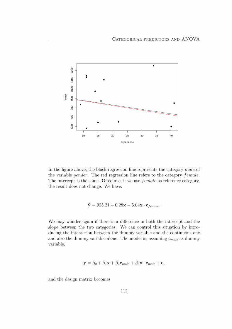
Categorical predictors and ANOVA
10 15 20 25 30 35 40
600
700
800
900
1000
1100
1200
experience
wag
e
In the figure above, the black regression line represents the category male ofthe variable gender. The red regression line refers to the category female.The intercept is the same. Of course, if we use female as reference category,the result does not change. We have:
y = 925.21 + 0.28x− 5.04x · cfemale.
We may wonder again if there is a difference in both the intercept and theslope between the two categories. We can control this situation by intro-ducing the interaction between the dummy variable and the continuous oneand also the dummy variable alone. The model is, assuming cmale as dummyvariable,
y = β0 + β1x + β3cmale + β3x · cmale + e,
and the design matrix becomes
112

8.1. Categorical predictors
(Intercept) x cmale x · cmale1 41 0 01 14 0 01 11 1 111 9 0 01 40 1 401 17 1 171 15 0 01 34 1 341 11 1 111 16 1 161 22 0 01 11 1 11
When cmale = 0, then the model is β0 + β1x. When instead cmale = 1, themodel is (β0 + β3) + (β2 + β4)x. The inclusion of the dummy variable haseffect on both the intercept and the slope. Let’s estimate the model by usingthe dummy cmale. We obtain
y = 788.64 + 0.14x + 233.80cmale − 3.57x · cmale.
It means that
y =
788.64 + 0.14x, if cmale = 0 hence, for a female
1022.44− 3.44x, ifcmale = 1 hence, for a male
113

Categorical predictors and ANOVA
10 15 20 25 30 35 40
600
700
800
900
1000
1100
1200
experience
wag
e
In the figure above, the black regression line represents the category male ofthe variable gender. The red regression line refers to the category female.Both intercept and slope are different. Of course, if we use female as refer-ence category, the result does not change. We have:
y = 1022.44− 3.44x− 233.80cfemale + 3.57x · cfemale.
Summarizing, indicating with c the dummy variable, we can have
1. The same regression line for both groups:
Y = β0 + β1x + ε
2. Separate regression lines for each group but same slope:
Y = β0 + β1x + β2c + ε
3. Separate regression lines for each group but same intercept:
Y = β0 + β1x + β2x · c + ε
4. Separate regression lines for each group:
Y = β0 + β1x + β2c + β3x · c + ε
114

8.2. Analysis Of Variance
8.1.1 Multiple categories
We can use dummy variables to control for something with multiple cate-gories, the rule is always the same: include as many dummy variables asthere are the categories of the categorical predictor minus one. If a cate-gorical predictor is, say, the geographical area of residence and include fourcategories, for example North, Center, South and Islands, then once thebaseline category has been chosen (for example North) the dummy variablecoding is
South Center IslandsNorth 0 0 0South 1 0 0
Center 0 1 0Islands 0 0 1
Any categorical variable can be turned into a set of dummy variables, thepredictor matrix can contain several categorical variables. If a particular pre-dictor contains many categories, it may make sense to group some together.The interactions can, of course, be made between categorical variables.
8.2 Analysis Of Variance
Analysis of Variance (ANOVA) is a category of statistical models used toanalyze the differences among group means in a sample. In its simplestform ANOVA generalizes the t-test beyond two means, providing a statisticaltest of whether two or more population means are equal. ANOVA can beviewed as a special case of multiple regression model, where the dependentvariable is regressed on only qualitative variables. The latter are generatedthrough dummy coding. Predictors are now typically called factors whichhave some number of levels. The parameters are often called effects. Whenthe parameters are considered fixed but unknown, ANOVA is said to be afixed-effects model. When parameters are taken to be random variables,model is said a random-effects model.ANOVA models are often employed to analyze data coming from plannedexperiments. In this case data are said to be derived from randomizationrather than random sampling. The experimental plan consists in a researchdesign in which two or more independent categorical variables (factors) aremeasured on all subjects. In factorial designs every single case belongs to agroup and the group is defined by the intersection of the categories defined bythe independent variables. In experimental plans (or designs), the statistician
115

Categorical predictors and ANOVA
varies in a controlled way the levels of one or more factors, to determine theirseffects on the variable of interest (the dependent variable or response variable)measured on the experimental units. The goal is to provide an answer to thefollowing questions:
1. what factors influence the response?Main effects analysis.
2. which combinations of factor levels affect the response?Interaction effects analysis.
Four assumptions underlie analysis of variance in it’s parametric view:
1. Random sampling from the source population;
2. Independent measures within each sample, yielding uncorrelated re-sponse residuals;
3. Homogeneous variances across all the sampled populations;
4. Normal distribution of the response residuals around the model.
Let’s start with the case in which we have a continuous variable y and onlyone factor, that we call x. In this case, we perform a one way ANOVA.
8.2.1 One way ANOVA
The variable x is assumed to be a factor with g categories. The interrelation-ship between y and x involves a comparison of the distribution of y amongthe g levels of x. We want to test that samples in all groups are drawn frompopulations with the same mean values.Let yij the ith observation on y taken in group j, where i = 1, 2, . . . , nj, j =1, 2, . . . , g and nj is the sample size within the jth group, with
∑gj=1 nj = n.
The sample means for the g groups are y.1, y.2, . . . , y.g, with y.j = 1nj
∑nji=1 yij.
The grand mean (the mean of all n observations) is y.. = 1n
∑gj=1
∑nji=1 yij =
(∑g
j=1 nj y.j)/n.
The model describing the behavior of y can be written as
yij = µj + εij i = 1, . . . , nj; j = 1, . . . , g;
where εij represents a random variable with mean 0 and variance σ2 withmutually independent components.
116

8.2. Analysis Of Variance
An alternative way to represent the model is
yij = µ+ αj + εij i = 1, . . . , nj; j = 1, . . . , g;
where∑g
j=1 αj = 0 and εij ∼ N(0, σ2).
The null hypothesis is
H0 : µ1 = µ2 = . . . µg = µ or equivalently αj = 0 ∀j = 1, . . . , g
against
H1 : µj 6= µ or equivalently αj 6= 0 for at least one level.
The total variation in y over the sample is the total sum of squares (SST):
SST =
g∑j=1
nj∑i=1
(yij − y..)2 =
nj∑i=1
y2ij − ny2...
The variation expressed by the fitted model is given by the sum of squaresbetween groups (SSB, sometimes called sum of squares among groups, SSA),that measures the variation among the group means. It is expressed by:
SSB =
g∑j=1
nj∑i=1
(y.j − y..)2 =
g∑j=1
nj (y.j − y..)2 .
The variation in the sample within group j gives the sum of squares withingroups (SSW):
SSW =
g∑j=1
nj∑i=1
(yij − y.j)2 =
g∑j=1
nj∑i=1
y2ij −g∑j=1
nj y2.j.
It is easy to check that SST=SSW+SSB. Under the assumption of homo-geneity of variance (homoscedasticity), the best unbiased estimator of σ2 isgiven by SSW/(n − g). Under H0, both SSB/(g − 1) and SSW/(n − g)provide independent estimates of σ2. Under the normality assumption theratio
F =SSB/(g − 1)
SSW/(n− g)
has a F distribution with g − 1 and n− g degrees of freedom.
117

Categorical predictors and ANOVA
Let’s see an example, taken by Jobson (1991, p.401). Table 8.1 shows datacoming from a marketing research for the monitoring of food purchases offamilies in several cities. A study was carried out to determine the effec-tiveness of four different advertisements (ads) designed to stimulate the con-sumption of milk products.
Ad.1 Ad.2 Ad.3 Ad.412.35 21.86 14.43 21.4420.52 42.17 22.26 31.2130.85 49.61 23.99 40.0939.35 63.65 36.98 55.6848.87 73.75 42.13 65.8158.01 85.95 54.19 76.6128.26 13.76 14.44 30.7837.67 24.59 29.63 45.7544.70 37.30 38.27 56.3757.54 49.53 51.59 70.1967.57 59.25 59.09 79.8177.70 67.68 71.69 94.2310.97 0.00 2.90 6.4626.70 2.41 17.28 18.6136.81 16.10 19.62 30.1451.34 22.71 29.53 39.1262.69 30.19 38.57 51.1572.68 41.64 48.20 59.110.00 11.90 4.48 27.624.52 27.75 18.01 42.63
13.71 42.22 21.96 59.2027.91 56.06 34.42 74.9238.57 66.16 40.14 92.3742.71 78.71 57.06 98.0213.11 8.00 10.90 14.3616.89 18.27 28.22 26.3727.99 27.72 38.62 34.1536.35 42.04 48.31 54.0248.85 48.50 60.23 59.9061.97 59.92 71.39 74.79
Table 8.1: Family expenditures on milk products
Are the expenditures of the families influenced by the type of advertising?
118

8.2. Analysis Of Variance
We can answer by performing a one way anova. Let’s compute the necessaryquantities:
Ad.1 Ad.2 Ad.3 Ad.4nj = 30 30 30 30
y.j = 1117.1630
= 37.24 1189.4030
= 39.65 1048.5330
= 34.95 1530.9130
= 51.03
SSWj =54080.85− 30 · 37.242
= 12479.30
63036.40− 30 · 39.652
= 15880.66
46919.98− 30 · 34.952
= 10272.80
95677.53− 30 · 51.032
= 17554.68
The gran mean is
y.. =
∑gj=1 nj y.j
n=
30 · 37.24 + 30 · 39.65 + 30 · 39.65 + 30 · 39.65
120= 40.72.
We can now compute the necessary quantities:
SSW = 12479.30 + 15880.66 + 15880.66 + 17554.68 = 56187.44
SSB = 30 · (37.24− 40.72)2 + 30 · (39.65− 40.72)2 + 30 · (34.95− 40.72)2 + 30 · (51.03− 40.72)2
= 4585.68
SST = SSB + SSW = 4585.68 + 56187.44 = 60773.12
The degrees of freedom are g− 1 for SSB, n− g for SSW and n− 1 for SST.The ANOVA table is
source df SS MS FBetween g − 1 SSB MSB = SSB/(g − 1) MSB/MSWWithin n− g SSW MSW = SSW/(n− g)Total n− 1 SST
hence, for our data
source df SS MS FBetween 3 4585.68 1528.56 3.16Within 116 56187.44 484.37Total 119 60773.12
The p-value for the F statistic of 3.16 with 3 and 116 degrees of freedomis equal to 0.0275. We conclude that there are some differences among themeans. Better, we can say that for at least one level of the experimentalfactor the mean is different from the grand mean.
119

Categorical predictors and ANOVA
1 2 3 4
020
4060
8010
0
AD
Exp
endi
ture
The figure above shows the boxplots of each distribution of y (Expendi-ture) within each level of x (Advertisements). We may wonder which level ofthe experimental design induced us to reject the null hypothesis. The figuresuggests us that, probably, the advertisement #4 has produced a level ofexpenditure larger than the average. To better investigate in this sense weneed the multiple comparisons, or the popst-hoc analysis.
8.2.2 Multiple comparisons
Multiple comparisons are procedure to answer to the question ”which groupshave different means?”. If we have g levels (g groups), then there are k =(g2
)= g(g−1)
2pairs of means to be compared. The post-hoc procedures are
based on k t-test (or on related confidence intervals). The problem is thatwith k simultaneous comparisons of pairs of means, if we set the probabilityof rejecting H0 (type I error) equal to α in each of the k tests, in the complexof the k comparisons we have a probability of committing a type I errorequal to 1− (1− α)k > α. For example if g = 4 and α = 0.05 we have that1− (1− 0.05)4 = 0.265, then the probability to have at least one significantdifference is no longer 0.05 but in fact it is equal to 0.265. For this reasonseveral procedures have been introduced in order to control the experimentalerror rate. Here, we recall the Bonferroni adjustment, for which, if there arek = (g(g − 1))/2 comparisons, for a given α this approach uses αo = α/k,hence the critical value of the t-test is tα0/2;(n−g) and not the usual tα/2;(n−g).
120

8.2. Analysis Of Variance
In our case we have, by using the Bonferroni adjustment, that the p-valuesfor the k = 6 comparisons of the 4 levels of x are
Ad.1 Ad.2 Ad.3Ad.2 1.000 - -Ad.3 1.000 1.000 -Ad.4 0.101 0.285 0.033
Then, there is evidence that AD4 causes the rejection of H0, being significantthe difference between AD3 and AD4.
8.2.3 Regression approach
What we have seen can be obtained as a special case of multiple regressionmodel by using only one categorical predictor. The response variable y andthe design matrix X are
y =
12.3520.52
...21.8642.17
...14.4322.26
...59.9074.79
; X =
1 0 0 · · · 01 0 0 · · · 0...
......
...1 1 0 · · · 01 1 0 · · · 0...
......
...1 0 1 · · · 01 0 1 · · · 0...
......
...1 0 0 · · · 11 0 0 · · · 1
,
where the columns of X represent the intercept, the dummy variable AD = 2,the dummy variable AD = 3 and the dummy variable AD = 4. Hence, wehave a categorical predictor with 4 categories, and we have put 3 dummy vari-ables in the model, by dropping the case AD = 1. The estimated regressionparameters are
Estimate Std. Error t value Pr(>|t|)(Intercept) 37.24 4.02 9.27 0.00
AD2 2.41 5.68 0.42 0.67AD3 -2.29 5.68 -0.40 0.69AD4 13.79 5.68 2.43 0.02
121
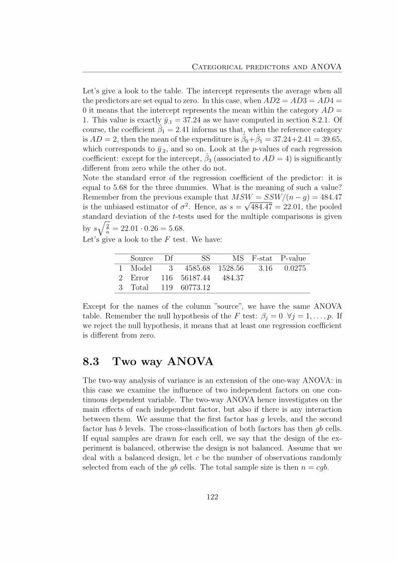
Categorical predictors and ANOVA
Let’s give a look to the table. The intercept represents the average when allthe predictors are set equal to zero. In this case, when AD2 = AD3 = AD4 =0 it means that the intercept represents the mean within the category AD =1. This value is exactly y.1 = 37.24 as we have computed in section 8.2.1. Ofcourse, the coefficient β1 = 2.41 informs us that, when the reference categoryis AD = 2, then the mean of the expenditure is β0+β1 = 37.24+2.41 = 39.65,which corresponds to y.2, and so on. Look at the p-values of each regressioncoefficient: except for the intercept, β3 (associated to AD = 4) is significantlydifferent from zero while the other do not.Note the standard error of the regression coefficient of the predictor: it isequal to 5.68 for the three dummies. What is the meaning of such a value?Remember from the previous example that MSW = SSW/(n− g) = 484.47is the unbiased estimator of σ2. Hence, as s =
√484.47 = 22.01, the pooled
standard deviation of the t-tests used for the multiple comparisons is given
by s√
2n
= 22.01 · 0.26 = 5.68.
Let’s give a look to the F test. We have:
Source Df SS MS F-stat P-value1 Model 3 4585.68 1528.56 3.16 0.02752 Error 116 56187.44 484.373 Total 119 60773.12
Except for the names of the column ”source”, we have the same ANOVAtable. Remember the null hypothesis of the F test: βj = 0 ∀j = 1, . . . , p. Ifwe reject the null hypothesis, it means that at least one regression coefficientis different from zero.
8.3 Two way ANOVA
The two-way analysis of variance is an extension of the one-way ANOVA: inthis case we examine the influence of two independent factors on one con-tinuous dependent variable. The two-way ANOVA hence investigates on themain effects of each independent factor, but also if there is any interactionbetween them. We assume that the first factor has g levels, and the secondfactor has b levels. The cross-classification of both factors has then gb cells.If equal samples are drawn for each cell, we say that the design of the ex-periment is balanced, otherwise the design is not balanced. Assume that wedeal with a balanced design, let c be the number of observations randomlyselected from each of the gb cells. The total sample size is then n = cgb.
122

8.3. Two way ANOVA
The model describing the behavior of y can be written as
yijh = µij + εijh i = 1, . . . , b; j = 1, . . . , g h = 1, . . . , c,
where εijh ∼ N(0, σ2).An alternative way to represent the model is
yijh = µ+ αj + βi + εijh i = 1, . . . , b; j = 1, . . . , g; h = 1, . . . , c,
where∑g
j=1 αj =∑b
i=1 βi =∑g
j=1 (αβ)ij =∑b
i=1 (αβ)ij = 0. The parame-ters (αβ)ij represent the interaction parameters. Three independent hypoth-esis testing can be made:
H01 : βj = 0 ∀j = 1, . . . , g ;
H02 : αi = 0 ∀i = 1, . . . , b ;
H03 : (αβ)ij = 0 ∀i = 1, . . . , b j = 1, . . . , g .
The following table shows how data are organized in a balanced design.
Factor 11 · j · g
Factor 2
1 y111, . . . , y11c · · · y1j1, . . . , y1jc · · · y1g1, . . . , y1gc
·...
......
i yi11, . . . , yi1c · · · yij1, . . . , yijc · · · yig1, . . . , yigc
·...
......
b yb11, . . . , yb1c · · · ybj1, . . . , ybjc · · · ybg1, . . . , ybgc
The quantities (sum of squares) to be computed to perform a two wayANOVA are:
SST =∑b
i=1
∑gj=1
∑ch1
(yijh − y...)2 =∑b
i=1
∑gj=1
∑ch1y2ijh− b ·c ·g · y2...
SSBf1 = b · c ·∑g
j=1 (y.j. − y...)2 = b · c ·∑g
j=1 y2.j. − b · c · g · y2...
SSBf2 = g · c ·∑b
i=1 (yi.. − y...)2 = g · c ·∑b
j=1 y2i.. − b · c · g · y2...
SSI = c ·∑b
i=1
∑gj=1 (yij. − yi.. − y.j. + y...)
2
SSE =∑b
i=1
∑gj=1
∑ch1
(yijh − yij.)2 =∑b
i=1
∑gj=1
∑ch1y2ijh−b·c·g · y2ij.
123

Categorical predictors and ANOVA
Let’s give a look to SSI, the sum of squares of the interaction term. It canbe expressed as
SSI = c ·b∑i=1
g∑j=1
(yij. − yi.. − y.j. + y...)2
= c ·b∑i=1
b∑j=1
y2ij. − b · c ·g∑j=1
y2.j. − g · c ·b∑i=1
y2i.. + b · g · c · y2...
By looking at the balanced two way model in terms of cell mean model
Factor 11 · j · g
Factor 2
1 y11. y1j. y1g. y1..·i yi1. yij. yig. yi..·b yb1. ybj. ybg. yb..
y.1. y.j. y.g. y...
it should be clear the the interaction effect
αβij = (yij. − yi..)− (y.j. − y...)= yij. − yi.. − y.j. + y...
= yij. − (yi.. − y...)− (y.j. − y...) + y...
evaluates the difference between each cell with its row marginal (differencebetween the blue highlighted quantities in the table above) with the columnmarginal and the grand mean (difference between the red highlighted quan-tities in the table above). If this difference is (statistically) different fromzero, then there is an interaction effect in that particular cell.
We have the necessary information to build the ANOVA table:
source df SS MS FFactor1 g − 1 SSBf1 MSBf1 = SSBf1/(g − 1) MSBf1/MSEFactor2 b− 1 SSBf2 MSBf2 = SSBf2/(b− 1) MSBf2/MSE
Interaction (g − 1)(b− 1) SSI MSI = SSI/(g − 1)(b− 1) MSI/MSEError bg(c− 1) SSE MSE = SSE/bg(c− 1)Total bgc− 1 SST
124

8.3. Two way ANOVA
In testing the hypotheses, we should examine H03 first. If we cannot rejectthis null hypothesis, then the interactions are not significant and the inter-action term can be dropped from the model. In this case, the error sum ofsquares will increase to SSE + SSI, as also the degrees of freedom of theerrors will increase to (bgc− g − b+ 1) (balanced two way ANOVA withoutinteraction). If one of the main effects (either Factor 1 or Factor 2) is notsignificant, it may also be dropped from the model without changing the esti-mates for the other main effect (One way ANOVA). If instead H03 is rejected,never remove a main effect even if it should be not significant.
Table 8.2 shows the data coming from the marketing research for the mon-itoring of food purchases introduced in section 8.2.1 in which the Region ofresidence is added.
Region Ad.1 Ad.2 Ad.3 Ad.41 12.35 21.86 14.43 21.441 20.52 42.17 22.26 31.211 30.85 49.61 23.99 40.091 39.35 63.65 36.98 55.681 48.87 73.75 42.13 65.811 58.01 85.95 54.19 76.612 28.26 13.76 14.44 30.782 37.67 24.59 29.63 45.752 44.70 37.30 38.27 56.372 57.54 49.53 51.59 70.192 67.57 59.25 59.09 79.812 77.70 67.68 71.69 94.233 10.97 0.00 2.90 6.463 26.70 2.41 17.28 18.613 36.81 16.10 19.62 30.143 51.34 22.71 29.53 39.123 62.69 30.19 38.57 51.153 72.68 41.64 48.20 59.114 0.00 11.90 4.48 27.624 4.52 27.75 18.01 42.634 13.71 42.22 21.96 59.204 27.91 56.06 34.42 74.924 38.57 66.16 40.14 92.374 42.71 78.71 57.06 98.025 13.11 8.00 10.90 14.365 16.89 18.27 28.22 26.375 27.99 27.72 38.62 34.155 36.35 42.04 48.31 54.025 48.85 48.50 60.23 59.905 61.97 59.92 71.39 74.79
Table 8.2: Family expenditures on milk products with ADs and Regrion
We can see that the four ADs have been proposed in 5 different regions.The design is balanced because each AD was proposed 6 times in each ofthe 5 regions. We already know that SST = 60773.12 and the grand meany... = 40.72. We know that c = 6, g = 4, b = 5 and n = 120. The following
125

Categorical predictors and ANOVA
table shows the same data represented in terms of cell means (remember thatc = 6 is a constant for each cell).
(Region/AD) Ad.1 Ad.2 Ad.3 Ad.4 means1 34.99 56.16 32.33 48.47 42.992 52.24 42.02 44.12 62.86 50.313 43.53 18.84 26.02 34.10 30.624 21.24 47.13 29.35 65.79 40.885 34.19 34.08 42.95 43.93 38.79
means 37.24 39.65 34.95 51.03 40.72
Now we can compute all the sums of squares. First, we compute the squareof the marginal means:
y2.j. = 1386.72, 1571.86, 1221.57, 2604.09
y2i.. = 1848.14, 2530.89, 937.71, 1670.94, 1504.37
y2... = 1657.85,
then we compute the square of each yij.,
1224.42 3154.51 1045.23 2349.662729.02 1765.54 1946.43 3950.751895.01 355.01 676.87 1162.70451.00 2221.55 861.13 4328.76
1169.18 1161.11 1844.27 1929.99
We are ready for compute all the necessary quantities:
SSAD = b · c ·g∑j=1
y2.j. − b · c · g · y2...
= 30 · (1386.72 + 1571.86 + 1221.57 + 2604.09)− 120 · 1657.85
= 4585.68
Of course, this quantity corresponds to the SSB we computed in performingthe one way anova in Section 8.2.1.
126

8.3. Two way ANOVA
SSRG = g · c ·b∑i=1
y2i.. − b · c · g · y2...
= 24 · (1848.14 + 2530.89 + 1221.57 + 1670.94 + 1504.37)− 120 · 1657.85
= 4867.51
SSI = c ·b∑i=1
b∑j=1
y2ij. − b · c ·g∑j=1
y2.j. − g · c ·b∑i=1
y2i.. + b · g · c · y2... =
= 6 · (1224.42 + 3154.51 + . . .+ 1929.99)−− 30 · (1386.72 + 1571.86 + 1221.57 + 2604.09)−− 24 · (1848.14 + 2530.89 + 937.71 + 1670.94 + 1670.94) +
+ 120 · 1657.85 =
= 8937.92
We have that SSE = SST − (SSAD +SSRG+SSI) = 60773.12− (4585.68 +4867.51 + 8937.92) = 42382.02.
The degrees of freedom are (g − 1) = 3 for AD, (b − 1) = 4 for Region,(b − 1)(g − 1) = 12 for the interaction, bg(c − 1) = 100 for the error andbcg − 1 = n− 1 = 119 for SST. We can build the ANOVA table:
source SS df MS F P-valueAD 4585.68 3 1528.56 3.61 0.0160Region 4867.51 4 1216.88 2.87 0.0268Interaction 8937.92 12 744.83 1.76 0.0658Error 42382.02 100 423.82Total 60773.12 119
By looking at the p-values of the three F-statistics we can conclude thatthere are significant differences among the ADs means and among the Re-gion means (if we set the probability of type-I error at 0.05). There is aweak interaction between AD and Region. Often it is useful to visualize theinteractions through a plot.
127
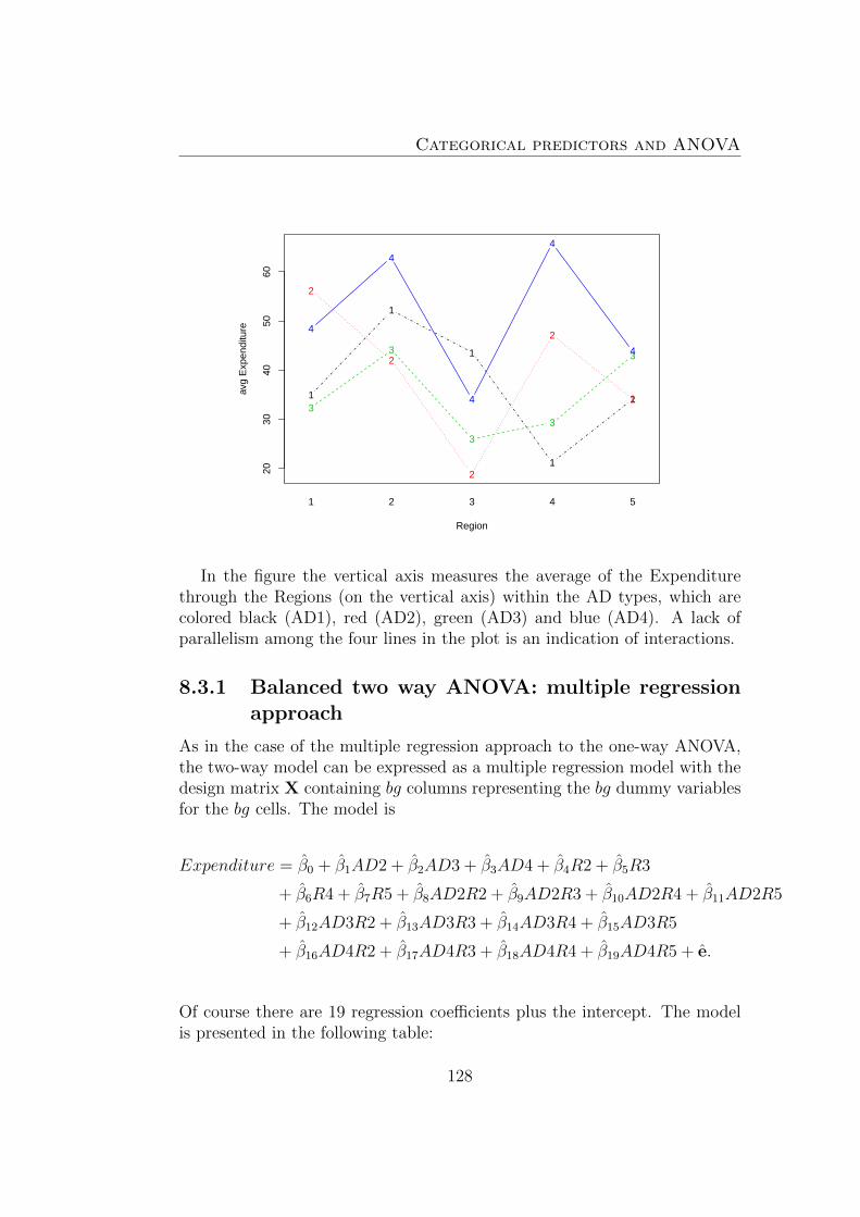
Categorical predictors and ANOVA
1
1
1
1
1
2030
4050
60
Region
avg
Exp
endi
ture
2
2
2
2
23
3
3
3
3
4
4
4
4
4
1 2 3 4 5
In the figure the vertical axis measures the average of the Expenditurethrough the Regions (on the vertical axis) within the AD types, which arecolored black (AD1), red (AD2), green (AD3) and blue (AD4). A lack ofparallelism among the four lines in the plot is an indication of interactions.
8.3.1 Balanced two way ANOVA: multiple regressionapproach
As in the case of the multiple regression approach to the one-way ANOVA,the two-way model can be expressed as a multiple regression model with thedesign matrix X containing bg columns representing the bg dummy variablesfor the bg cells. The model is
Expenditure = β0 + β1AD2 + β2AD3 + β3AD4 + β4R2 + β5R3
+ β6R4 + β7R5 + β8AD2R2 + β9AD2R3 + β10AD2R4 + β11AD2R5
+ β12AD3R2 + β13AD3R3 + β14AD3R4 + β15AD3R5
+ β16AD4R2 + β17AD4R3 + β18AD4R4 + β19AD4R5 + e.
Of course there are 19 regression coefficients plus the intercept. The modelis presented in the following table:
128

8.3. Two way ANOVA
Estimate Std. Error t value Pr(>|t|)(Intercept) 34.99 8.40 4.16 0.00
AD2 21.17 11.89 1.78 0.08AD3 -2.66 11.89 -0.22 0.82AD4 13.48 11.89 1.13 0.26
Region2 17.25 11.89 1.45 0.15Region3 8.54 11.89 0.72 0.47Region4 -13.76 11.89 -1.16 0.25Region5 -0.80 11.89 -0.07 0.95
AD2:Region2 -31.39 16.81 -1.87 0.06AD3:Region2 -5.46 16.81 -0.32 0.75AD4:Region2 -2.87 16.81 -0.17 0.86AD2:Region3 -45.86 16.81 -2.73 0.01AD3:Region3 -14.85 16.81 -0.88 0.38AD4:Region3 -22.91 16.81 -1.36 0.18AD2:Region4 4.72 16.81 0.28 0.78AD3:Region4 10.77 16.81 0.64 0.52AD4:Region4 31.08 16.81 1.85 0.07AD2:Region5 -21.29 16.81 -1.27 0.21AD3:Region5 11.41 16.81 0.68 0.50AD4:Region5 -3.74 16.81 -0.22 0.82
The twenty cell means can be obtained by adding together the appropriateparameter estimates: for example, β0 = 34.99 indicates the mean in the cellin which there is the situation AD1-Region 1, β0 + β1 = 56.16 indicates themean in the cell in which there is the situation AD2-Region 1, and so on.The two-way ANOVA testing procedure can be obtained through a series ofpartial F tests, with the following nested models:
model0 : Expenditure = β0 + e;
model1 : Expenditure = β0 + β1AD2 + β2AD3 + β3AD4 + e;
model2 : β0 + β1AD2 + β2AD3 + β3AD4 + β4R2 + β5R3 + β6R4 +β7R5 + e;
model3 : full model with the 20 regression parameters.
hence we have the following tests:
H0 : model1 is adequate vs model0:Res.Df RSS Df Sum of Sq F Pr(>F)
model0 119 60773.12model1 116 56187.44 3 4585.68 3.16 0.03
129

Categorical predictors and ANOVA
H0 : model2 is adequate vs model1:Res.Df RSS Df Sum of Sq F Pr(>F)
model0 119 60773.12model1 116 56187.44 3 4585.68 3.34 0.02model2 112 51319.93 4 4867.51 2.66 0.04
H0 : model3 is adequate vs model2:Res.Df RSS Df Sum of Sq F Pr(>F)
model0 119 60773.12model1 116 56187.44 3 4585.68 3.61 0.0160model2 112 51319.93 4 4867.51 2.87 0.0268model3 100 42382.02 12 8937.92 1.76 0.0658
The last test returns in fact the same ANOVA table displayed in last section,that for convenience we reproduce here:
source SS df MS F P-valueAD 4585.68 3 1528.56 3.61 0.0160Region 4867.51 4 1216.88 2.87 0.0268Interaction 8937.92 12 744.83 1.76 0.0658Error 42382.02 100 423.82Total 60773.12 119
By looking at the three partial ANOVA tables, the sum of squares of theeffects are always the same. The differences are, of course, in the ratiosleading to the mean of squares (MS) because both SSE and the relativedegrees of freedom are consequently updated.
8.3.2 ANOVA: considerations
When the observations follow Gaussian distributions with a common vari-ance, the F distribution provides the standard of comparison for the ratio ofthe two mean squares. What if the distribution of the observations is notGaussian? What can we say, or do?To check for normality the qqplot is a valid instrument. The one-way ANOVAis considered a robust test against the normality assumption. It tolerates vi-olations to its normality assumption rather well. The one-way ANOVA cantolerate data that is non-normal (skewed or kurtotic distributions) with onlya small effect on the Type I error rate. However, platykurtosis can have aprofound effect when your group sizes are small.About the hypothesis of homoscedasticity, different kind of tests of homo-geneity of variance have been proposed. One of this is the Bartlett ’s test.
130

8.3. Two way ANOVA
Let’s define
M =
g∑j=1
(nj − 1)lns2
s2jand
c =
(1
(3g − 1)
)( g∑j=1
1
nj − 1− 1∑g
j=1 nj − 1
),
where s2j is the sample variance in the group j, j = 1, . . . , g and s2 is the sam-ple variance of y. Under H0 : σ2
1 = . . . σ2j = . . . = σ2
g , the statistic M/(c+ 1)is distributed as a χ2 with g − 1 degrees of freedom.
Another test of homogeneity of variance that is commonly used when thedata are balanced is the Cochran’ C test. The critical vales of the statistic
C =SSWmax∑gj=1 SSWj
can be compared with the ones tabulated for given sample size n and levelof α.
Balanced experimental designs are quite robust to deviations from the as-sumption of equal variances. In any case, non-parametric ANOVA (for ex-ample the Kruskall-Wallis ANOVA) as well as data transformation (for ex-ample log transformation, Box-Cox transformation, etc.) can be used whenthere are strong violations.
Most of the time balanced experimental designs are used because ANOVAshould follow a controlled experiment. Researchers should control the factorsand the levels of the factors. Nevertheless, ANOVA sometimes is a ”simple”test of difference among means. Experimental designs can be unbalanced.The case of one way ANOVA is quite trivial for unbalanced model. In un-balanced two way ANOVA we can take in account unbalanced models.
There exists of course multiway ANOVA, we can set up contrasts to comparethe means over the levels of more factors, etc. Analysis of Variance andExperimental Design is a topic that, probably, you will study in a future.
131

Categorical predictors and ANOVA
8.4 Practical examples
8.4.1 Regression with categorical predictors
Let’s see an example on the autompg data set, coming from https://archive.
ics.uci.edu/ml/datasets/auto+mpg, that contains technical specificationof cars. The data set, slightly modified with respect to the original version,can be loaded by typing
> load("autompg.rda")
The variables are:
mpg, miles per gallon;
cyl, number of cylinders;
disp, displacement in cubic inches;
hp, power of the engine;
wt, weight;
acc, acceleration
year, model year;
origin, either ”domestic” or ”foreign” car
name, name and model of the car.
There are n = 383 statistical units. We are interested in check if the fuelefficiency in miles per gallon (mpg) depends on the displacement in cubicinches (disp) and the origin of the car (origin). The following code willdisplay the scatter plot.
> plot(mpg~disp, data=autompg)
132

8.4. Practical examples
100 200 300 400
1020
3040
disp
mpg
The variable origin is set as ”factor” with two categories:
> class(autompg$origin)
[1] "factor"
Let’s estimate a model with different intercepts and constant slope:
> autom1 <- lm(mpg~disp+origin, data=autompg)
> summary(autom1)
Call:
lm(formula = mpg ~ disp + origin, data = autompg)
Residuals:
Min 1Q Median 3Q Max
-10.559 -2.904 -0.576 2.434 18.814
Coefficients:
Estimate Std. Error t value Pr(>|t|)
(Intercept) 34.186242 0.777845 43.950 <2e-16 ***
disp -0.057251 0.002907 -19.696 <2e-16 ***
originforeign 1.300402 0.632372 2.056 0.0404 *
133

Categorical predictors and ANOVA
---
Signif. codes: 0 '***' 0.001 '**' 0.01 '*' 0.05 '.' 0.1 ' ' 1
Residual standard error: 4.506 on 380 degrees of freedom
Multiple R-squared: 0.6721, Adjusted R-squared: 0.6704
F-statistic: 389.5 on 2 and 380 DF, p-value: < 2.2e-16
From the summary of the model, we see that the reference category isdomestic. We can control the reference category with the the functionrelevel(). The following command changes the reference category of thevariable origin within the dataframe autompg:
> #first, we duplicate the autompg data set and we call it auto
> auto <- autompg
> #then we use the function relevel
> auto <- within(auto, origin <- relevel(origin, ref = "foreign"))
> #we estimate the same model as before,
> #just changing the reference category
> autom1_bis <- lm(mpg~disp+origin, data=auto)
> summary(autom1_bis)
Call:
lm(formula = mpg ~ disp + origin, data = auto)
Residuals:
Min 1Q Median 3Q Max
-10.559 -2.904 -0.576 2.434 18.814
Coefficients:
Estimate Std. Error t value Pr(>|t|)
(Intercept) 35.486645 0.489885 72.439 <2e-16 ***
disp -0.057251 0.002907 -19.696 <2e-16 ***
origindomestic -1.300402 0.632372 -2.056 0.0404 *
---
Signif. codes: 0 '***' 0.001 '**' 0.01 '*' 0.05 '.' 0.1 ' ' 1
Residual standard error: 4.506 on 380 degrees of freedom
Multiple R-squared: 0.6721, Adjusted R-squared: 0.6704
F-statistic: 389.5 on 2 and 380 DF, p-value: < 2.2e-16
In the first case (model autom1), the intercept is the mean of mpg within thecategory domestic when disp = 0. In the second case, the intercept is the
134

8.4. Practical examples
mean of mpg within the category foreign when disp = 0. Now we use thefunction abline(), that add a line to an existing plot. In this case we need oftwo inputs: the intercept and the slope:
> #intercept of domestic
> intdom <- autom1$coefficients[1]
> #intercept of foreign, the sum of
> #first and third coefficient
> intfor <- autom1$coefficients[1]+autom1$coefficients[3]
> #common splope
> auto1slope <- autom1$coefficients[2]
> plot(mpg~disp, data=autompg)
> #regression line for domestic cars, in black
> abline(intdom, auto1slope, col=1)
> #regression line for foreign cars, in red
> abline(intfor, auto1slope, col=2)
100 200 300 400
1020
3040
disp
mpg
Let’s now estimate a model with common intercept and different slopes:
> autom2 <- lm(mpg~disp+disp:origin, data=autompg)
> summary(autom2)
135

Categorical predictors and ANOVA
Call:
lm(formula = mpg ~ disp + disp:origin, data = autompg)
Residuals:
Min 1Q Median 3Q Max
-10.0829 -2.9707 -0.5226 2.2375 18.6119
Coefficients:
Estimate Std. Error t value Pr(>|t|)
(Intercept) 35.3411019 0.7307472 48.363 <2e-16 ***
disp -0.0608894 0.0027679 -21.999 <2e-16 ***
disp:originforeign 0.0009044 0.0054985 0.164 0.869
---
Signif. codes: 0 '***' 0.001 '**' 0.01 '*' 0.05 '.' 0.1 ' ' 1
Residual standard error: 4.53 on 380 degrees of freedom
Multiple R-squared: 0.6685, Adjusted R-squared: 0.6668
F-statistic: 383.1 on 2 and 380 DF, p-value: < 2.2e-16
in this case, we have the common intercept and a slope for domestic (−0.061)and another for foreign (−0.061 +−0.061 = −0.060).
> #common intercept
> intboth <- autom2$coefficients[1]
> #slope for domestic
> slopedom2 <- autom2$coefficients[2]
> #slope for foreign
> slopefor2 <- autom2$coefficients[2]+autom2$coefficients[3]
> plot(mpg~disp, data=autompg)
> #regression line for domestic cars, in black
> abline(intboth, slopedom2, col=1)
> #regression line for foreign cars, in red
> abline(intboth, slopefor2, col=2)
136
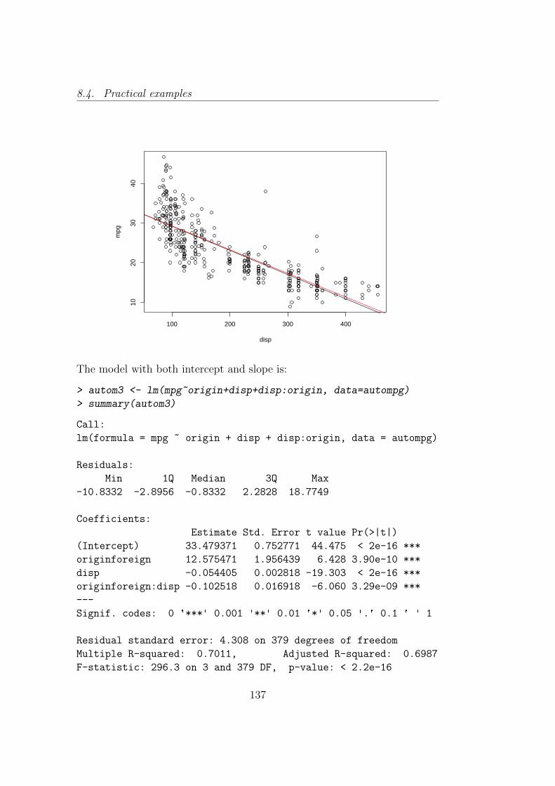
8.4. Practical examples
100 200 300 400
1020
3040
disp
mpg
The model with both intercept and slope is:
> autom3 <- lm(mpg~origin+disp+disp:origin, data=autompg)
> summary(autom3)
Call:
lm(formula = mpg ~ origin + disp + disp:origin, data = autompg)
Residuals:
Min 1Q Median 3Q Max
-10.8332 -2.8956 -0.8332 2.2828 18.7749
Coefficients:
Estimate Std. Error t value Pr(>|t|)
(Intercept) 33.479371 0.752771 44.475 < 2e-16 ***
originforeign 12.575471 1.956439 6.428 3.90e-10 ***
disp -0.054405 0.002818 -19.303 < 2e-16 ***
originforeign:disp -0.102518 0.016918 -6.060 3.29e-09 ***
---
Signif. codes: 0 '***' 0.001 '**' 0.01 '*' 0.05 '.' 0.1 ' ' 1
Residual standard error: 4.308 on 379 degrees of freedom
Multiple R-squared: 0.7011, Adjusted R-squared: 0.6987
F-statistic: 296.3 on 3 and 379 DF, p-value: < 2.2e-16
137

Categorical predictors and ANOVA
The intercepts and the slopes are:
> #Intercept for domestic cars
> intdom3 <- autom3$coefficients[1]
> #slope for domestic cars
> slopedom3 <- autom3$coefficients[3]
> #intercept for foreign cars
> intfor3 <- autom3$coefficients[1]+autom3$coefficients[2]
> #slope for foreign cars
> slopefor3 <- autom3$coefficients[3]+autom3$coefficients[4]
> plot(mpg~disp, data=autompg)
> #regression line for domestic cars, in black
> abline(intdom3, slopedom3, col=1)
> #regression line for foreign cars, in red
> abline(intfor3, slopefor3, col=2)
100 200 300 400
1020
3040
disp
mpg
In order to show an example with factors with more than two levels weconsider, on the same data, a model in which mpg is assumed to depend ondisp and the number of cylinders (cyl), which has been coded as a factor withthree levels (4, 6 and 8 cylinders). We directly estimate the more ”complex”model with different intercepts and different slopes:
138

8.4. Practical examples
> autom4 <- lm(mpg~disp+cyl+disp:cyl, data=autompg)
> summary(autom4)
Call:
lm(formula = mpg ~ disp + cyl + disp:cyl, data = autompg)
Residuals:
Min 1Q Median 3Q Max
-10.9133 -2.4642 -0.4301 2.1488 20.1082
Coefficients:
Estimate Std. Error t value Pr(>|t|)
(Intercept) 43.59052 1.55595 28.015 < 2e-16 ***
disp -0.13069 0.01396 -9.362 < 2e-16 ***
cyl6 -13.20026 3.49865 -3.773 0.000187 ***
cyl8 -20.85706 3.44362 -6.057 3.36e-09 ***
disp:cyl6 0.08299 0.01991 4.168 3.81e-05 ***
disp:cyl8 0.10817 0.01651 6.550 1.89e-10 ***
---
Signif. codes: 0 '***' 0.001 '**' 0.01 '*' 0.05 '.' 0.1 ' ' 1
Residual standard error: 4.169 on 377 degrees of freedom
Multiple R-squared: 0.7215, Adjusted R-squared: 0.7178
F-statistic: 195.4 on 5 and 377 DF, p-value: < 2.2e-16
Note that the syntax disp : cyl allows the interaction between disp and cyl.Let’s isolate intercepts and slopes:
> #Intercept for 4 cylinders cars
> int4cyl <- autom4$coefficients[1]
> #slope for 4 cylinders cars
> slope4cyl <- autom4$coefficients[2]
> #intercept for 6 cylinders cars
> int6cyl <- autom4$coefficients[1]+autom4$coefficients[3]
> #slope for 6 cylinders cars
> slope6cyl <- autom4$coefficients[2]+autom4$coefficients[5]
> #intercept for 8 cylinders cars
> int8cyl <- autom4$coefficients[1]+autom4$coefficients[4]
> #slope for 6 cylinders cars
> slope8cyl <- autom4$coefficients[2]+autom4$coefficients[6]
139

Categorical predictors and ANOVA
> plot(mpg~disp, data=autompg)
> #regression line for 4 cylinders cars, in black
> abline(int4cyl, slope4cyl, col=1)
> #regression line for 4 cylinders cars, in red
> abline(int6cyl, slope6cyl, col=2)
> #regression line for 4 cylinders cars, in green
> abline(int8cyl, slope8cyl, col=3)
100 200 300 400
1020
3040
disp
mpg
8.4.2 One way ANOVA
As an example of a one way ANOVA in R, we use the tires data. Here, wemay see if different brands of car tire have the same performance in terms ofmileage.
> load("tires.rda")
First, let’s visualize our data
> plot(Mileage~Brands, data=tires)
140

8.4. Practical examples
Apollo Bridgestone CEAT Falken
2830
3234
3638
40
Brands
Mile
age
Now we immediately perform the Bartlett’s test of homogeneity of variance:
> bt <- bartlett.test(Mileage~Brands, data=tires)
> bt
Bartlett test of homogeneity of variances
data: Mileage by Brands
Bartlett's K-squared = 2.1496, df = 3, p-value = 0.5419
We cannot reject the null hypothesis of homogeneity of the variance. We canvisualize the qqplot:
> qqnorm(tires$Mileage)
> qqline(tires$Mileage)
141

Categorical predictors and ANOVA
−2 −1 0 1 2
2830
3234
3638
40
Normal Q−Q Plot
Theoretical Quantiles
Sam
ple
Qua
ntile
s
There is no evidence of assumptions violation. We can proceed with themodel using the aov() function:
> oneway_anova_tires <- aov(Mileage~Brands, data=tires)
> summary(oneway_anova_tires)
Df Sum Sq Mean Sq F value Pr(>F)
Brands 3 256.3 85.43 17.94 2.78e-08 ***
Residuals 56 266.6 4.76
---
Signif. codes: 0 '***' 0.001 '**' 0.01 '*' 0.05 '.' 0.1 ' ' 1
If we want perform the model by using a multiple regression approach, firstwe estimate the model
> regoneway_anova_tires <- lm(Mileage~Brands, data=tires)
> #only the intercept
> regoneway_anova_tires1 <- lm(Mileage~1, data=tires)
> summary(regoneway_anova_tires)
Call:
lm(formula = Mileage ~ Brands, data = tires)
142

8.4. Practical examples
Residuals:
Min 1Q Median 3Q Max
-4.3337 -1.3848 0.0295 1.5336 6.2888
Coefficients:
Estimate Std. Error t value Pr(>|t|)
(Intercept) 34.79913 0.56342 61.764 < 2e-16 ***
BrandsBridgestone -3.01900 0.79679 -3.789 0.000372 ***
BrandsCEAT -0.03793 0.79679 -0.048 0.962205
BrandsFalken 2.82553 0.79679 3.546 0.000798 ***
---
Signif. codes: 0 '***' 0.001 '**' 0.01 '*' 0.05 '.' 0.1 ' ' 1
Residual standard error: 2.182 on 56 degrees of freedom
Multiple R-squared: 0.4901, Adjusted R-squared: 0.4628
F-statistic: 17.94 on 3 and 56 DF, p-value: 2.781e-08
then we can do a partial F test
> anova(regoneway_anova_tires1,regoneway_anova_tires)
Analysis of Variance Table
Model 1: Mileage ~ 1
Model 2: Mileage ~ Brands
Res.Df RSS Df Sum of Sq F Pr(>F)
1 59 522.94
2 56 266.65 3 256.29 17.942 2.781e-08 ***
---
Signif. codes: 0 '***' 0.001 '**' 0.01 '*' 0.05 '.' 0.1 ' ' 1
We are ready for the post-hoc test. We proceed with the Bonferroni adjust-ment using the pairwise.t.test() function:
143

Categorical predictors and ANOVA
> pairwise.t.test(tires$Mileage, tires$Brands, p.adj = "bonf")
Pairwise comparisons using t tests with pooled SD
data: tires$Mileage and tires$Brands
Apollo Bridgestone CEAT
Bridgestone 0.0022 - -
CEAT 1.0000 0.0026 -
Falken 0.0048 5.8e-09 0.0041
P value adjustment method: bonferroni
The multiple comparisons show that Apollo and CEAT return the same per-formance in terms of mean. Both are statistically different from Falken andBridgeston, and the latter are different in mean from each other.
8.4.3 Two way ANOVA
As an example of a two way ANOVA we analyze the rats data set, that isa study about rat survival times by treatment and poison from the pack-age faraway, in which 48 rats were allocated to 3 poisons (I,II,III) and 4treatments (A,B,C,D). The response was survival time in tens of hour
> data("rats")
First, let’s give a look to the plots:
> #divide the graphical window in order to do a sub-plot
> par(mfrow=c(1,2))
> plot(time ~ treat, data=rats)
> plot(time ~ poison, data=rats)
144

8.4. Practical examples
A B C D
0.2
0.4
0.6
0.8
1.0
1.2
treat
time
I II III
0.2
0.4
0.6
0.8
1.0
1.2
poison
time
We use the aov() function to perform the two way ANOVA
> twoway_anova_rats <- aov(time ~ poison+treat+poison:treat, data=rats)
> summary(twoway_anova_rats)
Df Sum Sq Mean Sq F value Pr(>F)
poison 2 1.0330 0.5165 23.222 3.33e-07 ***
treat 3 0.9212 0.3071 13.806 3.78e-06 ***
poison:treat 6 0.2501 0.0417 1.874 0.112
Residuals 36 0.8007 0.0222
---
Signif. codes: 0 '***' 0.001 '**' 0.01 '*' 0.05 '.' 0.1 ' ' 1
As it can be seen the interaction effect is not significant. The interaction plotcan be done by using the function interaction.plot().
> interaction.plot(rats$poison, rats$treat,
+ rats$time, col = c(1, 2, 3, 4), xlab = "Poison",
+ ylab = "avg Time")
145

Categorical predictors and ANOVA
0.2
0.3
0.4
0.5
0.6
0.7
0.8
0.9
Poison
avg
Tim
e
I II III
rats$treat
BDCA
Also graphically, there is not evidence of interaction effect. The two wayanova in terms of multiple regression approach can be done using the lm()function.
> #model with intercept
> rat0 <- lm(time ~ 1, data=rats)
> #model with one affact
> rat1 <- lm(time ~ poison, data=rats)
> #model with 2 effects
> rat2 <- lm(time ~ poison+treat, data=rats)
> #model with the interaction effect
> rat3 <- lm(time ~ poison+treat+poison:treat, data=rats)
146

8.4. Practical examples
> anova(rat0,rat1,rat2,rat3)
Analysis of Variance Table
Model 1: time ~ 1
Model 2: time ~ poison
Model 3: time ~ poison + treat
Model 4: time ~ poison + treat + poison:treat
Res.Df RSS Df Sum of Sq F Pr(>F)
1 47 3.00508
2 45 1.97207 2 1.03301 23.2217 3.331e-07 ***
3 42 1.05086 3 0.92121 13.8056 3.777e-06 ***
4 36 0.80073 6 0.25014 1.8743 0.1123
---
Signif. codes: 0 '***' 0.001 '**' 0.01 '*' 0.05 '.' 0.1 ' ' 1
The final model is then a two way ANOVA without interactions:
> twoway_anova_final <- aov(time ~ poison+treat, data=rats)
> summary(twoway_anova_final)
Df Sum Sq Mean Sq F value Pr(>F)
poison 2 1.0330 0.5165 20.64 5.7e-07 ***
treat 3 0.9212 0.3071 12.27 6.7e-06 ***
Residuals 42 1.0509 0.0250
---
Signif. codes: 0 '***' 0.001 '**' 0.01 '*' 0.05 '.' 0.1 ' ' 1
147


Bibliography
Belsley, D. A., Kuh, E., & Welsch, R. E. (2005). Regression diagnostics:Identifying influential data and sources of collinearity . John Wiley & Sons.
Chatterjee, S., & Hadi, A. S. (2015). Regression analysis by example. JohnWiley & Sons.
Chatterjee, S., & Simonoff, J. S. (2013). Handbook of regression analysis .John Wiley & Sons.
Draper, N. R., & Smith, H. (1998). Applied regression analysis . John Wiley& Sons.
Faraway, J. J. (2002). Practical regression and ANOVA using R., vol. 168.University of Bath Bath.URL https://cran.r-project.org/doc/contrib/Faraway-PRA.pdf
Faraway, J. J. (2005). Linear models with R.. Taylor & Francis.
Hadi, S. (1992). A new measure of overall potential influence in linear re-gression Computational Statistics & Data Analysis . 14(1), 1–27.
Hoaglin, D. C., Mosteller, F., & Tukey, J. W. (1991). Fundamentals ofexploratory analysis of variance, vol. 261. John Wiley & Sons.
Hocking, R. R. (2003). Methods and applications of linear models: regressionand the analysis of variance. John Wiley & Sons.
Janke, S. J., & Tinsley, F. (2005). Introduction to linear models and statisticalinference. John Wiley & Sons.
Jobson, J. (1991). Applied Multivariate Data Analysis. Volume I: Regressionand Experimental Design. New York: Springer.
Paradis, E. (2010). R for beginners.URL https://cran.r-project.org/doc/contrib/Paradis-rdebuts_
en.pdf
149

Bibliography
Piccolo, D. (2010). Statistica. Il mulino.
R Development Core Team (2006). R: A Language and Environment forStatistical Computing . R Foundation for Statistical Computing, Vienna,Austria. ISBN 3-900051-07-0.URL http://www.R-project.org
Seber, G. A., & Lee, A. J. (2012). Linear regression analysis. John Wiley &Sons.
Weisberg, S. (2005). Applied linear regression. John Wiley & Sons.
150