Lecture Notes in Financial Econometrics (MBF, MSc course …dl4a.org/uploads/pdf/FinEcmtAll.pdf ·...
267
Lecture Notes in Financial Econometrics (MBF, MSc course at UNISG) Paul Söderlind 1 26 May 2011 1 University of St. Gallen. Address: s/bf-HSG, Rosenbergstrasse 52, CH-9000 St. Gallen, Switzerland. E-mail: [email protected]. Document name: FinEcmtAll.TeX
Transcript of Lecture Notes in Financial Econometrics (MBF, MSc course …dl4a.org/uploads/pdf/FinEcmtAll.pdf ·...

Lecture Notes in Financial Econometrics (MBF,MSc course at UNISG)
Paul Söderlind1
26 May 2011
1University of St. Gallen. Address: s/bf-HSG, Rosenbergstrasse 52, CH-9000 St. Gallen,Switzerland. E-mail: [email protected]. Document name: FinEcmtAll.TeX

Contents
1 Review of Statistics 41.1 Random Variables and Distributions . . . . . . . . . . . . . . . . . . 41.2 Moments . . . . . . . . . . . . . . . . . . . . . . . . . . . . . . . . 101.3 Distributions Commonly Used in Tests . . . . . . . . . . . . . . . . . 131.4 Normal Distribution of the Sample Mean as an Approximation . . . . 16
A Statistical Tables 18
2 Least Squares Estimation 212.1 Least Squares . . . . . . . . . . . . . . . . . . . . . . . . . . . . . . 212.2 Hypothesis Testing . . . . . . . . . . . . . . . . . . . . . . . . . . . 352.3 Heteroskedasticity . . . . . . . . . . . . . . . . . . . . . . . . . . . . 402.4 Autocorrelation . . . . . . . . . . . . . . . . . . . . . . . . . . . . . 43
A A Primer in Matrix Algebra 45
A Statistical Tables 51
3 Index Models 543.1 The Inputs to a MV Analysis . . . . . . . . . . . . . . . . . . . . . . 543.2 Single-Index Models . . . . . . . . . . . . . . . . . . . . . . . . . . 553.3 Estimating Beta . . . . . . . . . . . . . . . . . . . . . . . . . . . . . 603.4 Multi-Index Models . . . . . . . . . . . . . . . . . . . . . . . . . . . 623.5 Principal Component Analysis . . . . . . . . . . . . . . . . . . . . . 653.6 Estimating Expected Returns . . . . . . . . . . . . . . . . . . . . . . 683.7 Estimation on Subsamples . . . . . . . . . . . . . . . . . . . . . . . 693.8 Robust Estimation� . . . . . . . . . . . . . . . . . . . . . . . . . . . 70
1

4 Testing CAPM and Multifactor Models 774.1 Market Model . . . . . . . . . . . . . . . . . . . . . . . . . . . . . . 774.2 Several Factors . . . . . . . . . . . . . . . . . . . . . . . . . . . . . 874.3 Fama-MacBeth� . . . . . . . . . . . . . . . . . . . . . . . . . . . . . 90
A Statistical Tables 93
5 Time Series Analysis 965.1 Descriptive Statistics . . . . . . . . . . . . . . . . . . . . . . . . . . 965.2 White Noise . . . . . . . . . . . . . . . . . . . . . . . . . . . . . . . 975.3 Autoregression (AR) . . . . . . . . . . . . . . . . . . . . . . . . . . 985.4 Moving Average (MA) . . . . . . . . . . . . . . . . . . . . . . . . . 1075.5 ARMA(p,q) . . . . . . . . . . . . . . . . . . . . . . . . . . . . . . . 1075.6 VAR(p) . . . . . . . . . . . . . . . . . . . . . . . . . . . . . . . . . 1085.7 Non-stationary Processes . . . . . . . . . . . . . . . . . . . . . . . . 110
6 Predicting Asset Returns 1176.1 Asset Prices, Random Walks, and the Efficient Market Hypothesis . . 1176.2 Autocorrelations . . . . . . . . . . . . . . . . . . . . . . . . . . . . 1216.3 Other Predictors and Methods . . . . . . . . . . . . . . . . . . . . . 1296.4 Security Analysts . . . . . . . . . . . . . . . . . . . . . . . . . . . . 1326.5 Technical Analysis . . . . . . . . . . . . . . . . . . . . . . . . . . . 1376.6 Spurious Regressions and In-Sample Overfit� . . . . . . . . . . . . . 1406.7 Empirical U.S. Evidence on Stock Return Predictability . . . . . . . . 145
7 Maximum Likelihood Estimation 1507.1 Maximum Likelihood . . . . . . . . . . . . . . . . . . . . . . . . . . 1507.2 Key Properties of MLE . . . . . . . . . . . . . . . . . . . . . . . . . 1557.3 Three Test Principles . . . . . . . . . . . . . . . . . . . . . . . . . . 1577.4 QMLE� . . . . . . . . . . . . . . . . . . . . . . . . . . . . . . . . . 157
8 ARCH and GARCH 1598.1 Heteroskedasticity . . . . . . . . . . . . . . . . . . . . . . . . . . . . 1598.2 ARCH Models . . . . . . . . . . . . . . . . . . . . . . . . . . . . . 1648.3 GARCH Models . . . . . . . . . . . . . . . . . . . . . . . . . . . . 167
2

8.4 Non-Linear Extensions . . . . . . . . . . . . . . . . . . . . . . . . . 1698.5 (G)ARCH-M . . . . . . . . . . . . . . . . . . . . . . . . . . . . . . 1718.6 Multivariate (G)ARCH . . . . . . . . . . . . . . . . . . . . . . . . . 172
9 Risk Measures 1769.1 Symmetric Dispersion Measures . . . . . . . . . . . . . . . . . . . . 1769.2 Downside Risk . . . . . . . . . . . . . . . . . . . . . . . . . . . . . 1789.3 Empirical Return Distributions . . . . . . . . . . . . . . . . . . . . . 188
10 Return Distributions (Univariate) 19110.1 Estimating and Testing Distributions . . . . . . . . . . . . . . . . . . 19110.2 Tail Distribution . . . . . . . . . . . . . . . . . . . . . . . . . . . . . 203
11 Return Distributions (Multivariate) 21311.1 Recap of Univariate Distributions . . . . . . . . . . . . . . . . . . . 21311.2 Exceedance Correlations . . . . . . . . . . . . . . . . . . . . . . . . 21411.3 Beyond (Linear) Correlations . . . . . . . . . . . . . . . . . . . . . . 21511.4 Copulas . . . . . . . . . . . . . . . . . . . . . . . . . . . . . . . . . 22111.5 Joint Tail Distribution . . . . . . . . . . . . . . . . . . . . . . . . . . 228
12 Option Pricing and Estimation of Continuous Time Processes 23512.1 The Black-Scholes Model . . . . . . . . . . . . . . . . . . . . . . . . 23512.2 Estimation of the Volatility of a Random Walk Process . . . . . . . . 243
13 Event Studies 25013.1 Basic Structure of Event Studies . . . . . . . . . . . . . . . . . . . . 25013.2 Models of Normal Returns . . . . . . . . . . . . . . . . . . . . . . . 25213.3 Testing the Abnormal Return . . . . . . . . . . . . . . . . . . . . . . 25513.4 Quantitative Events . . . . . . . . . . . . . . . . . . . . . . . . . . . 258
14 Kernel Density Estimation and Regression 25914.1 Non-Parametric Regression . . . . . . . . . . . . . . . . . . . . . . . 25914.2 Examples of Non-Parametric Estimation . . . . . . . . . . . . . . . . 265
3

.D..3
1 Review of Statistics
More advanced material is denoted by a star (�). It is not required reading.
1.1 Random Variables and Distributions
1.1.1 Distributions
A univariate distribution of a random variable x describes the probability of differentvalues. If f .x/ is the probability density function, then the probability that x is betweenA and B is calculated as the area under the density function from A to B
Pr .A � x < B/ DZ B
A
f .x/dx: (1.1)
See Figure 1.1 for illustrations of normal (gaussian) distributions.
Remark 1.1 If x � N.�; �2/, then the probability density function is
f .x/ D 1p2��2
e�12.x��� /
2
:
This is a bell-shaped curve centered on the mean � and where the standard deviation �
determines the “width” of the curve.
A bivariate distribution of the random variables x and y contains the same informationas the two respective univariate distributions, but also information on how x and y arerelated. Let h .x; y/ be the joint density function, then the probability that x is betweenA and B and y is between C and D is calculated as the volume under the surface of thedensity function
Pr .A � x < B and C � x < D/ DZ B
A
Z D
C
h.x; y/dxdy: (1.2)
4

−4 −3 −2 −1 0 1 2 3 40
0.1
0.2
0.3
0.4
N(0,2) distribution
x
Pr(−2 < x ≤ −1) = 16 %
Pr(0 < x ≤ 1) = 26 %
−4 −3 −2 −1 0 1 2 3 40
0.1
0.2
0.3
0.4
Normal distributions
x
N(0,2)
N(1,2)
−4 −3 −2 −1 0 1 2 3 40
0.1
0.2
0.3
0.4
Normal distributions
x
N(0,2)
N(0,1)
Figure 1.1: A few different normal distributions
A joint normal distributions is completely described by the means and the covariancematrix "
x
y
#� N
"�x
�y
#;
"�2x �xy
�xy �2y
#!; (1.3)
where �x and �y denote means of x and y, �2x and �2y denote the variances of x andy and �xy denotes their covariance. Some alternative notations are used: E x for themean, Std.x/ for the standard deviation, Var.x/ for the variance and Cov.x; y/ for thecovariance.
Clearly, if the covariance �xy is zero, then the variables are (linearly) unrelated to eachother. Otherwise, information about x can help us to make a better guess of y. See Figure1.2 for an example. The correlation of x and y is defined as
�xy D �xy
�x�y: (1.4)
5

If two random variables happen to be independent of each other, then the joint densityfunction is just the product of the two univariate densities (here denoted f .x/ and k.y/)
h.x; y/ D f .x/ k .y/ if x and y are independent. (1.5)
This is useful in many cases, for instance, when we construct likelihood functions formaximum likelihood estimation.
−2 −1 0 1 20
0.2
0.4
N(0,1) distribution
x
−2
0
2
−20
20
0.1
0.2
x
Bivariate normal distribution, corr=0.1
y
−2
0
2
−20
20
0.1
0.2
x
Bivariate normal distribution, corr=0.8
y
Figure 1.2: Density functions of univariate and bivariate normal distributions
1.1.2 Conditional Distributions�
If h .x; y/ is the joint density function and f .x/ the (marginal) density function of x, thenthe conditional density function is
g.yjx/ D h.x; y/=f .x/: (1.6)
6

For the bivariate normal distribution (1.3) we have the distribution of y conditional on agiven value of x as
yjx � N��y C �xy
�2x.x � �x/ ; �2y �
�xy�xy
�2x
�: (1.7)
Notice that the conditional mean can be interpreted as the best guess of y given that weknow x. Similarly, the conditional variance can be interpreted as the variance of theforecast error (using the conditional mean as the forecast). The conditional and marginaldistribution coincide if y is uncorrelated with x. (This follows directly from combining(1.5) and (1.6)). Otherwise, the mean of the conditional distribution depends on x, andthe variance is smaller than in the marginal distribution (we have more information). SeeFigure 1.3 for an illustration.
−2
0
2
−20
20
0.1
0.2
x
Bivariate normal distribution, corr=0.1
y −2 −1 0 1 20
0.2
0.4
0.6
0.8
Conditional distribution of y, corr=0.1
x=−0.8
x=0
y
−2
0
2
−20
20
0.1
0.2
x
Bivariate normal distribution, corr=0.8
y −2 −1 0 1 20
0.2
0.4
0.6
0.8
Conditional distribution of y, corr=0.8
x=−0.8
x=0
y
Figure 1.3: Density functions of normal distributions
7

1.1.3 Illustrating a Distribution
If we know that type of distribution (uniform, normal, etc) a variable has, then the bestway of illustrating the distribution is to estimate its parameters (mean, variance and what-ever more—see below) and then draw the density function.
In case we are not sure about which distribution to use, the first step is typically to drawa histogram: it shows the relative frequencies for different bins (intervals). For instance, itcould show the relative frequencies of a variable xt being in each of the follow intervals:-0.5 to 0, 0 to 0.5 and 0.5 to 1.0. Clearly, the relative frequencies should sum to unity (or100%), but they are sometimes normalized so the area under the histogram has an area ofunity (as a distribution has).
See Figure 1.4 for an illustration.
−20 −10 0 10 200
0.05
0.1Histogram of small growth stocks
mean, std: 0.44 8.44skew, kurt, BJ: 0.5 6.9 436.7
Monthly excess return, %
−20 −10 0 10 200
0.05
0.1Histogram of large value stocks
mean, std: 0.69 5.00skew, kurt, BJ: 0.1 5.5 171.0
Monthly excess return, %
Monthly data on two U.S. indices, 1957:1−2010:9
Sample size: 645
Figure 1.4: Histogram of returns, the curve is a normal distribution with the same meanand standard deviation as the return series
1.1.4 Confidence Bands and t-tests
Confidence bands are typically only used for symmetric distributions. For instance, a 90%confidence band is constructed by finding a critical value c such that
Pr .� � c � x < �C c/ D 0:9: (1.8)
8

Replace 0.9 by 0.95 to get a 95% confidence band—and similarly for other levels. Inparticular, if x � N.�; �2/, then
Pr .� � 1:65� � x < �C 1:65�/ D 0:9 and
Pr .� � 1:96� � x < �C 1:96�/ D 0:95: (1.9)
As an example, suppose x is not a data series but a regression coefficient (denotedO)—and we know that the standard error equals some number � . We could then construct
a 90% confidence band around the point estimate as
Œ O � 1:65�; O C 1:65��: (1.10)
In case this band does not include zero, then we would be 90% that the (true) regressioncoefficient is different from zero.
Alternatively, suppose we instead construct the 90% confidence band around zero as
Œ0 � 1:65�; 0C 1:65��: (1.11)
If this band does not include the point estimate ( O), then we are also 90% sure that the(true) regression coefficient is different from zero. This latter approach is virtually thesame as doing a t-test, that, by checking ifˇ
ˇ O � 0�ˇˇ > 1:65: (1.12)
To see that, notice that if (1.12) holds, then
O < �1:65� or O > 1:65�; (1.13)
which is the same as O being outside the confidence band in (1.11).
9

1.2 Moments
1.2.1 Mean and Standard Deviation
The mean and variance of a series are estimated as
Nx DPTtD1xt=T and O�2 DPT
tD1 .xt � Nx/2 =T: (1.14)
The standard deviation (here denoted Std.xt/), the square root of the variance, is the mostcommon measure of volatility. (Sometimes we use T �1 in the denominator of the samplevariance instead T .) See Figure 1.4 for an illustration.
A sample mean is normally distributed if xt is normal distributed, xt � N.�; �2/. Thebasic reason is that a linear combination of normally distributed variables is also normallydistributed. However, a sample average is typically approximately normally distributedeven if the variable is not (discussed below). If xt is iid (independently and identicallydistributed), then the variance of a sample mean is
Var. Nx/ D �2=T , if xt is iid. (1.15)
A sample average is (typically) unbiased, that is, the expected value of the sampleaverage equals the population mean, that is,
E Nx D E xt D �: (1.16)
Since sample averages are typically normally distributed in large samples (according tothe central limit theorem), we thus have
Nx � N.�; �2=T /; (1.17)
so we can construct a t-stat ast D Nx � �
�=pT; (1.18)
which has an N.0; 1/ distribution.
10

Proof. (of (1.15)–(1.16)) To prove (1.15), notice that
Var. Nx/ D Var�PT
tD1xt=T�
DPTtD1 Var .xt=T /
D T Var .xt/ =T 2
D �2=T:
The first equality is just a definition and the second equality follows from the assumptionthat xt and xs are independently distributed. This means, for instance, that Var.x2 Cx3/ D Var.x2/ C Var.x3/ since the covariance is zero. The third equality follows fromthe assumption that xt and xs are identically distributed (so their variances are the same).The fourth equality is a trivial simplification.
To prove (1.16)
E Nx D EPT
tD1xt=T
DPTtD1 E xt=T
D E xt :
The first equality is just a definition and the second equality is always true (the expectationof a sum is the sum of expectations), and the third equality follows from the assumptionof identical distributions which implies identical expectations.
1.2.2 Skewness and Kurtosis
The skewness, kurtosis and Bera-Jarque test for normality are useful diagnostic tools.They are
Test statistic Distributionskewness D 1
T
PTtD1
�xt��
�
�3N .0; 6=T /
kurtosis D 1T
PTtD1
�xt��
�
�4N .3; 24=T /
Bera-Jarque D T6
skewness2 C T24.kurtosis � 3/2 �22:
(1.19)
This is implemented by using the estimated mean and standard deviation. The distribu-tions stated on the right hand side of (1.19) are under the null hypothesis that xt is iidN.�; �2/. The “excess kurtosis” is defined as the kurtosis minus 3. The test statistic for
11
the normality test (Bera-Jarque) can be compared with 4.6 or 6.0, which are the 10% and5% critical values of a �22 distribution.
Clearly, we can test the skewness and kurtosis by traditional t-stats as in
t D skewnessp6=T
and t D kurtosis � 3p24=T
; (1.20)
which both have N.0; 1/ distribution under the null hypothesis of a normal distribution.See Figure 1.4 for an illustration.
1.2.3 Covariance and Correlation
The covariance of two variables (here x and y) is typically estimated as
O�xy DPT
tD1 .xt � Nx/ .yt � Ny/ =T: (1.21)
(Sometimes we use T � 1 in the denominator of the sample covariance instead of T .)The correlation of two variables is then estimated as
O�xy D O�xyO�x O�y ; (1.22)
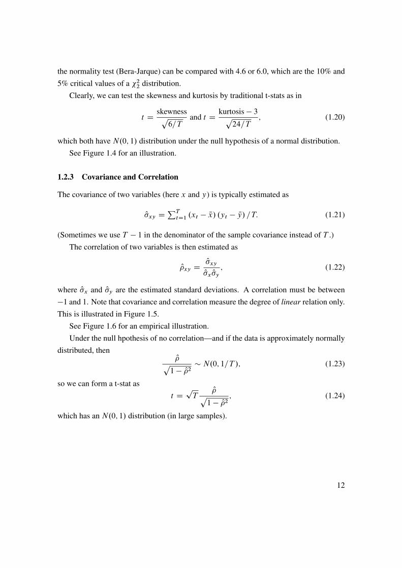
where O�x and O�y are the estimated standard deviations. A correlation must be between�1 and 1. Note that covariance and correlation measure the degree of linear relation only.This is illustrated in Figure 1.5.
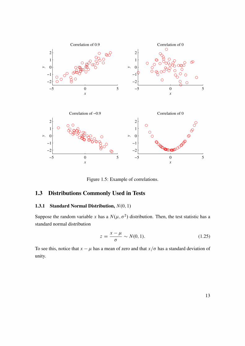
See Figure 1.6 for an empirical illustration.Under the null hpothesis of no correlation—and if the data is approximately normally
distributed, thenO�p
1 � O�2� N.0; 1=T /; (1.23)
so we can form a t-stat ast DpT
O�p1 � O�2
; (1.24)
which has an N.0; 1/ distribution (in large samples).
12
−5 0 5
−2
−1
0
1
2
Correlation of 0.9
x
y
−5 0 5
−2
−1
0
1
2
Correlation of 0
x
y
−5 0 5
−2
−1
0
1
2
Correlation of −0.9
x
y
−5 0 5
−2
−1
0
1
2
Correlation of 0
x
y
Figure 1.5: Example of correlations.
1.3 Distributions Commonly Used in Tests
1.3.1 Standard Normal Distribution, N.0; 1/
Suppose the random variable x has a N.�; �2/ distribution. Then, the test statistic has astandard normal distribution
z D x � ��� N.0; 1/: (1.25)
To see this, notice that x �� has a mean of zero and that x=� has a standard deviation ofunity.
13
−25 −20 −15 −10 −5 0 5 10 15 20 25−25
−20
−15
−10
−5
0
5
10
15
20
25
Small growth stocks, montly returns, %
Lar
ge
val
ue
stock
s, m
ontl
y r
eturn
s, %
Monthly data on two U.S. indices 1957:1−2010:9
Correlation: 0.56
Figure 1.6: Scatter plot of two different portfolio returns
1.3.2 t -distribution
If we instead need to estimate � to use in (1.25), then the test statistic has tdf -distribution
t D x � �O� � tn; (1.26)
where n denotes the “degrees of freedom,” that is the number of observations minus thenumber of estimated parameters. For instance, if we have a sample with T data pointsand only estimate the mean, then n D T � 1.
The t-distribution has more probability mass in the tails: gives a more “conservative”test (harder to reject the null hypothesis), but the difference vanishes as the degrees offreedom (sample size) increases. See Figure 1.7 for a comparison and Table A.1 forcritical values.
Example 1.2 (t -distribution) If t D 2:0 and n D 50, then this is larger than the10%
critical value (but not the 5% critical value) for a 2-sided test in Table A.1.
14

−3 −2 −1 0 1 2 30
0.1
0.2
0.3
0.4N(0,1) and t(10) distributions
x
10% crit val:
1.641.81
N(0,1)
t(10)
−3 −2 −1 0 1 2 30
0.1
0.2
0.3
0.4N(0,1) and t(50) distributions
x
1.641.68
N(0,1)
t(50)
0 2 4 6 8 10 120
0.1
0.2
0.3
0.4
Chi−square(n) distributions
x
4.619.24
n=2
n=5
0 1 2 3 4 50
0.5
1F(n,50) distributions
x
2.411.97
n=2
n=5
Figure 1.7: Probability density functions
1.3.3 Chi-square Distribution
If z � N.0; 1/, then z2 � �21, that is, z2 has a chi-square distribution with one degree offreedom. This can be generalized in several ways. For instance, if x � N.�x; �xx/ andy � N.�y; �yy/ and they are uncorrelated, then Œ.x ��x/=�x�2C Œ.y ��y/=�y�2 � �22.
More generally, we have
v0˙�1v � �2n, if the n � 1 vector v � N.0;˙/: (1.27)
See Figure 1.7 for an illustration and Table A.2 for critical values.
Example 1.3 (�22 distribution) Suppose x is a 2 � 1 vector"x1
x2
#� N
"4
2
#;
"5 3
3 4
#!:
15

If x1 D 3 and x2 D 5, then"3 � 45 � 2
#0 "5 3
3 4
#�1 "3 � 45 � 2
#� 6:1
has a � �22 distribution. Notice that 6.1 is higher than the 5% critical value (but not the
1% critical value) in Table A.2.
1.3.4 F -distribution
If we instead need to estimate ˙ in (1.27) and let n1 be the number of elements in v(previously called just n), then
v0 O �1v=n1 � Fn1;n2 (1.28)
where Fn1;n2 denotes an F -distribution with (n1; n2) degrees of freedom. Similar to the t -distribution, n2 is the number of observations minus the number of estimated parameters.See Figure 1.7 for an illustration and Tables A.3–A.4 for critical values.
1.4 Normal Distribution of the Sample Mean as an Approximation
In many cases, it is unreasonable to just assume that the variable is normally distributed.The nice thing with a sample mean (or sample average) is that it will still be normallydistributed—at least approximately (in a reasonably large sample). This section givesa short summary of what happens to sample means as the sample size increases (oftencalled “asymptotic theory”)
The law of large numbers (LLN) says that the sample mean converges to the truepopulation mean as the sample size goes to infinity. This holds for a very large classof random variables, but there are exceptions. A sufficient (but not necessary) conditionfor this convergence is that the sample average is unbiased (as in (1.16)) and that thevariance goes to zero as the sample size goes to infinity (as in (1.15)). (This is also calledconvergence in mean square.) To see the LLN in action, see Figure 1.8.
The central limit theorem (CLT) says thatpT Nx converges in distribution to a normal
distribution as the sample size increases. See Figure 1.8 for an illustration. This alsoholds for a large class of random variables—and it is a very useful result since it allows
16

−2 −1 0 1 20
1
2
3Distribution of sample avg.
T=5 T=25 T=100
Sample average
−6 −4 −2 0 2 4 60
0.1
0.2
0.3
0.4
Distribution of √T × sample avg.
√T × sample average
Sample average of zt−1 where z
t has a χ2
(1) distribution
Figure 1.8: Sampling distributions
us to test hypothesis. Most estimators (including least squares and other methods) areeffectively some kind of sample average, so the CLT can be applied.
17

A Statistical Tables
n Critical values10% 5% 1%
10 1.81 2.23 3.1720 1.72 2.09 2.8530 1.70 2.04 2.7540 1.68 2.02 2.7050 1.68 2.01 2.6860 1.67 2.00 2.6670 1.67 1.99 2.6580 1.66 1.99 2.6490 1.66 1.99 2.63100 1.66 1.98 2.63Normal 1.64 1.96 2.58
Table A.1: Critical values (two-sided test) of t distribution (different degrees of freedom)and normal distribution.
18

n Critical values10% 5% 1%
1 2.71 3.84 6.632 4.61 5.99 9.213 6.25 7.81 11.344 7.78 9.49 13.285 9.24 11.07 15.096 10.64 12.59 16.817 12.02 14.07 18.488 13.36 15.51 20.099 14.68 16.92 21.6710 15.99 18.31 23.21
Table A.2: Critical values of chisquare distribution (different degrees of freedom, n).
n1 n2 �2n1=n1
10 30 50 100 3001 4.96 4.17 4.03 3.94 3.87 3.842 4.10 3.32 3.18 3.09 3.03 3.003 3.71 2.92 2.79 2.70 2.63 2.604 3.48 2.69 2.56 2.46 2.40 2.375 3.33 2.53 2.40 2.31 2.24 2.216 3.22 2.42 2.29 2.19 2.13 2.107 3.14 2.33 2.20 2.10 2.04 2.018 3.07 2.27 2.13 2.03 1.97 1.949 3.02 2.21 2.07 1.97 1.91 1.8810 2.98 2.16 2.03 1.93 1.86 1.83
Table A.3: 5% Critical values of Fn1;n2 distribution (different degrees of freedom).
19

n1 n2 �2n1=n1
10 30 50 100 3001 3.29 2.88 2.81 2.76 2.72 2.712 2.92 2.49 2.41 2.36 2.32 2.303 2.73 2.28 2.20 2.14 2.10 2.084 2.61 2.14 2.06 2.00 1.96 1.945 2.52 2.05 1.97 1.91 1.87 1.856 2.46 1.98 1.90 1.83 1.79 1.777 2.41 1.93 1.84 1.78 1.74 1.728 2.38 1.88 1.80 1.73 1.69 1.679 2.35 1.85 1.76 1.69 1.65 1.6310 2.32 1.82 1.73 1.66 1.62 1.60
Table A.4: 10% Critical values of Fn1;n2 distribution (different degrees of freedom).
20

.D..3
2 Least Squares Estimation
Reference: Verbeek (2008) 2 and 4More advanced material is denoted by a star (�). It is not required reading.
2.1 Least Squares
2.1.1 Simple Regression: Constant and One Regressor
The simplest regression model is
yt D ˇ0 C ˇ1xt C ut , where Eut D 0 and Cov.xt ; ut/ D 0; (2.1)
where we can observe (have data on) the dependent variable yt and the regressor xt butnot the residual ut . In principle, the residual should account for all the movements in ytthat we cannot explain (by xt ).
Note the two very important assumptions: (i) the mean of the residual is zero; and(ii) the residual is not correlated with the regressor, xt . If the regressor summarizes allthe useful information we have in order to describe yt , then the assumptions imply thatwe have no way of making a more intelligent guess of ut (even after having observed xt )than that it will be zero.
Suppose you do not know ˇ0 or ˇ1, and that you have a sample of data: yt and xt fort D 1; :::; T . The LS estimator of ˇ0 and ˇ1 minimizes the loss functionPT
tD1.yt � b0 � b1xt/2 D .y1 � b0 � b1x1/2 C .y2 � b0 � b1x2/2 C :::: (2.2)
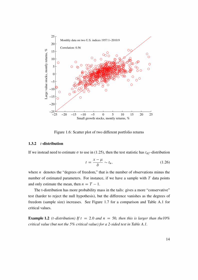
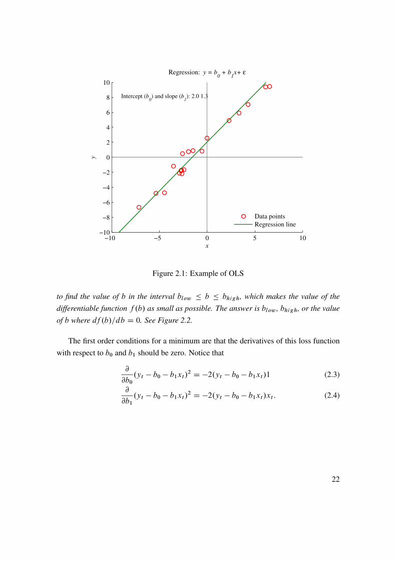
by choosing b0 and b1 to make the loss function value as small as possible. The objectiveis thus to pick values of b0 and b1 in order to make the model fit the data as closelyas possible—where close is taken to be a small variance of the unexplained part (theresidual). See Figure 2.1 for an illustration.
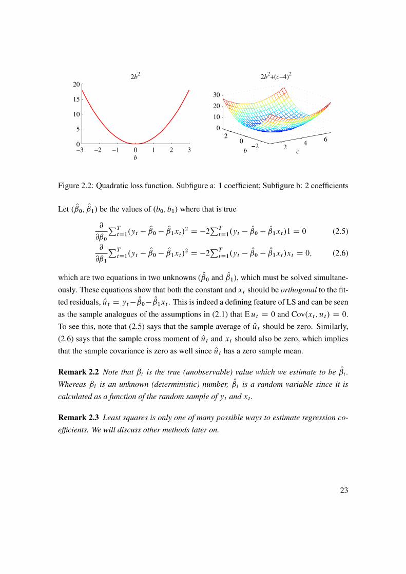
Remark 2.1 (First order condition for minimizing a differentiable function). We want
21
−10 −5 0 5 10−10
−8
−6
−4
−2
0
2
4
6
8
10
Regression: y = b0 + b
1x+ ε
x
y
Intercept (b0) and slope (b
1): 2.0 1.3
Data points
Regression line
Figure 2.1: Example of OLS
to find the value of b in the interval blow � b � bhigh, which makes the value of the
differentiable function f .b/ as small as possible. The answer is blow , bhigh, or the value
of b where df .b/=db D 0. See Figure 2.2.
The first order conditions for a minimum are that the derivatives of this loss functionwith respect to b0 and b1 should be zero. Notice that
@
@b0.yt � b0 � b1xt/2 D �2.yt � b0 � b1xt/1 (2.3)
@
@b1.yt � b0 � b1xt/2 D �2.yt � b0 � b1xt/xt : (2.4)
22
−3 −2 −1 0 1 2 30
5
10
15
20
2b2
b
24
6−2
02
0
10
20
30
c
2b2+(c−4)
2
b
Figure 2.2: Quadratic loss function. Subfigure a: 1 coefficient; Subfigure b: 2 coefficients
Let . O0; O1/ be the values of .b0; b1/ where that is true
@
@ˇ0
PTtD1.yt � O0 � O1xt/2 D �2
PTtD1.yt � O0 � O1xt/1 D 0 (2.5)
@
@ˇ1
PTtD1.yt � O0 � O1xt/2 D �2
PTtD1.yt � O0 � O1xt/xt D 0; (2.6)
which are two equations in two unknowns ( O0 and O1), which must be solved simultane-ously. These equations show that both the constant and xt should be orthogonal to the fit-ted residuals, Out D yt� O0� O1xt . This is indeed a defining feature of LS and can be seenas the sample analogues of the assumptions in (2.1) that Eut D 0 and Cov.xt ; ut/ D 0.To see this, note that (2.5) says that the sample average of Out should be zero. Similarly,(2.6) says that the sample cross moment of Out and xt should also be zero, which impliesthat the sample covariance is zero as well since Out has a zero sample mean.
Remark 2.2 Note that ˇi is the true (unobservable) value which we estimate to be Oi .Whereas ˇi is an unknown (deterministic) number, Oi is a random variable since it is
calculated as a function of the random sample of yt and xt .
Remark 2.3 Least squares is only one of many possible ways to estimate regression co-
efficients. We will discuss other methods later on.
23
−1 −0.5 0 0.5 1
−2
−1
0
1
2
OLS, y = b0 + b
1x + u, b
0=0
Data
2*x
OLS
x
y
y: −1.5 −0.6 2.1
x: −1.0 0.0 1.0
0 1 2 3 40
5
10Sum of squared errors
b1
b1: 1.8
R2: 0.92
Std(b1): 0.30
−1 −0.5 0 0.5 1
−2
−1
0
1
2
OLS
x
y
y: −1.3 −1.0 2.3
x: −1.0 0.0 1.0
0 1 2 3 40
5
10Sum of squared errors
b1
b1: 1.8
R2: 0.81
Std(b1): 0.50
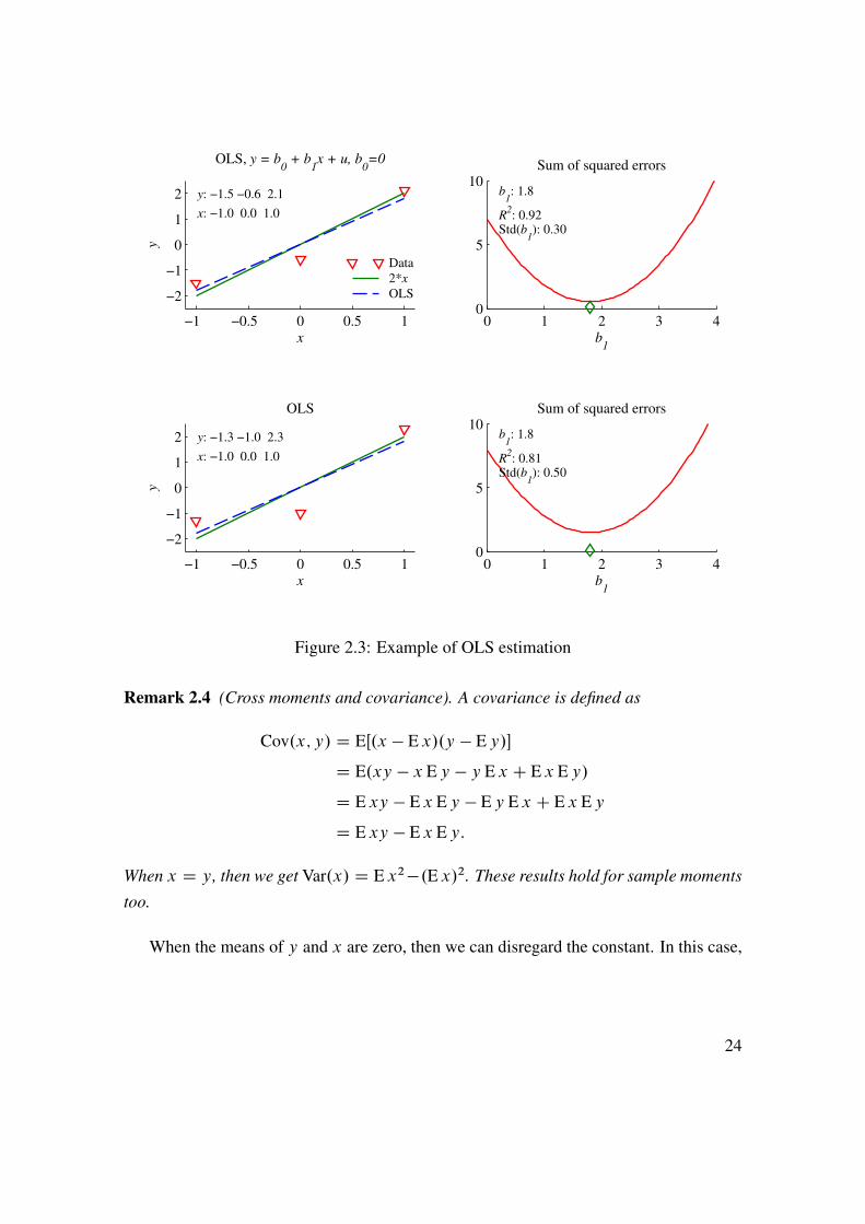
Figure 2.3: Example of OLS estimation
Remark 2.4 (Cross moments and covariance). A covariance is defined as
Cov.x; y/ D EŒ.x � E x/.y � Ey/�
D E.xy � x Ey � y E x C E x Ey/
D E xy � E x Ey � Ey E x C E x Ey
D E xy � E x Ey:
When x D y, then we get Var.x/ D E x2�.E x/2. These results hold for sample moments
too.
When the means of y and x are zero, then we can disregard the constant. In this case,
24

−30 −20 −10 0 10 20 30−30
−20
−10
0
10
20
30Scatter plot against market return
Excess return %, market
Exce
ss r
eturn
%, H
iTec
US data 1970:1−2010:9
α
β
−0.14 1.28
−30 −20 −10 0 10 20 30−30
−20
−10
0
10
20
30Scatter plot against market return
Excess return %, market
Exce
ss r
eturn
%, U
tils
α
β
0.22 0.53
Figure 2.4: Scatter plot against market return
(2.6) with O0 D 0 immediately givesPTtD1ytxt D O1
PTtD1xtxt or
O1 D
PTtD1 ytxt=TPTtD1 xtxt=T
: (2.7)
In this case, the coefficient estimator is the sample covariance (recall: means are zero) ofyt and xt , divided by the sample variance of the regressor xt (this statement is actuallytrue even if the means are not zero and a constant is included on the right hand side—justmore tedious to show it).
See Table 2.1 and Figure 2.4 for illustrations.
2.1.2 Least Squares: Goodness of Fit
The quality of a regression model is often measured in terms of its ability to explain themovements of the dependent variable.
Let Oyt be the fitted (predicted) value of yt . For instance, with (2.1) it would be Oyt DO0 C O1xt . If a constant is included in the regression (or the means of y and x are zero),
then a check of the goodness of fit of the model is given by
R2 D Corr.yt ; Oyt/2: (2.8)
25
HiTec Utils
constant -0.14 0.22(-0.87) (1.42)
market return 1.28 0.53(32.27) (12.55)
R2 0.75 0.35obs 489.00 489.00Autocorr (t) -0.76 0.84White 6.83 19.76All slopes 364.82 170.92
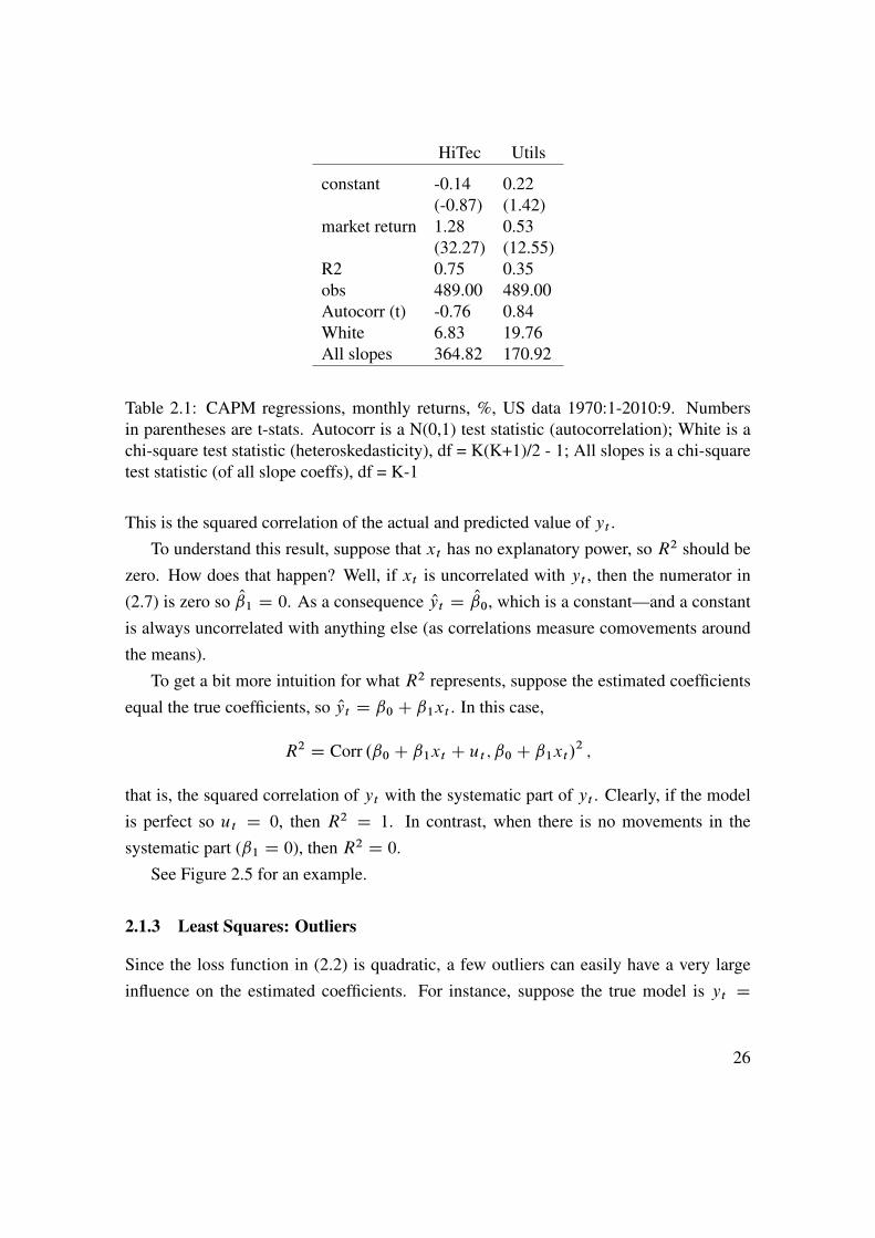
Table 2.1: CAPM regressions, monthly returns, %, US data 1970:1-2010:9. Numbersin parentheses are t-stats. Autocorr is a N(0,1) test statistic (autocorrelation); White is achi-square test statistic (heteroskedasticity), df = K(K+1)/2 - 1; All slopes is a chi-squaretest statistic (of all slope coeffs), df = K-1
This is the squared correlation of the actual and predicted value of yt .To understand this result, suppose that xt has no explanatory power, so R2 should be
zero. How does that happen? Well, if xt is uncorrelated with yt , then the numerator in(2.7) is zero so O1 D 0. As a consequence Oyt D O0, which is a constant—and a constantis always uncorrelated with anything else (as correlations measure comovements aroundthe means).
To get a bit more intuition for what R2 represents, suppose the estimated coefficientsequal the true coefficients, so Oyt D ˇ0 C ˇ1xt . In this case,
R2 D Corr .ˇ0 C ˇ1xt C ut ; ˇ0 C ˇ1xt/2 ;
that is, the squared correlation of yt with the systematic part of yt . Clearly, if the modelis perfect so ut D 0, then R2 D 1. In contrast, when there is no movements in thesystematic part (ˇ1 D 0), then R2 D 0.
See Figure 2.5 for an example.
2.1.3 Least Squares: Outliers
Since the loss function in (2.2) is quadratic, a few outliers can easily have a very largeinfluence on the estimated coefficients. For instance, suppose the true model is yt D
26

HiTec Utils
constant 0.14 0.00(1.07) (0.02)
market return 1.11 0.66(30.31) (16.22)
SMB 0.23 -0.18(4.15) (-3.49)
HML -0.58 0.46(-9.67) (6.90)
R2 0.82 0.48obs 489.00 489.00Autocorr (t) 0.39 0.97White 65.41 50.09All slopes 402.69 234.62
Table 2.2: Fama-French regressions, monthly returns, %, US data 1970:1-2010:9. Num-bers in parentheses are t-stats. Autocorr is a N(0,1) test statistic (autocorrelation); Whiteis a chi-square test statistic (heteroskedasticity), df = K(K+1)/2 - 1; All slopes is a chi-square test statistic (of all slope coeffs), df = K-1
0:75xt C ut , and that the residual is very large for some time period s. If the regressioncoefficient happened to be 0.75 (the true value, actually), the loss function value would belarge due to the u2t term. The loss function value will probably be lower if the coefficientis changed to pick up the ys observation—even if this means that the errors for the otherobservations become larger (the sum of the square of many small errors can very well beless than the square of a single large error).
There is of course nothing sacred about the quadratic loss function. Instead of (2.2)one could, for instance, use a loss function in terms of the absolute value of the error˙TtD1 jyt � ˇ0 � ˇ1xt j. This would produce the Least Absolute Deviation (LAD) estima-
tor. It is typically less sensitive to outliers. This is illustrated in Figure 2.7. However, LSis by far the most popular choice. There are two main reasons: LS is very easy to computeand it is fairly straightforward to construct standard errors and confidence intervals for theestimator. (From an econometric point of view you may want to add that LS coincideswith maximum likelihood when the errors are normally distributed.)
27

0 20 40 60
−0.5
0
0.5
Return = a + b*lagged Return, slope
Return horizon (months)
Slope with 90% conf band
US stock returns 1926:1−2010:4
0 20 40 600
0.05
0.1
Return = a + b*lagged Return, R2
Return horizon (months)
0 20 40 600
0.2
0.4
0.6Return = a + b*E/P, slope
Return horizon (months)
0 20 40 600
0.05
0.1
0.15Return = a + b*E/P, R
2
Return horizon (months)
Figure 2.5: Predicting US stock returns (various investment horizons) with the dividend-price ratio
2.1.4 The Distribution of O
Note that the estimated coefficients are random variables since they depend on which par-ticular sample that has been “drawn.” This means that we cannot be sure that the estimatedcoefficients are equal to the true coefficients (ˇ0 and ˇ1 in (2.1)). We can calculate an es-timate of this uncertainty in the form of variances and covariances of O0 and O1. Thesecan be used for testing hypotheses about the coefficients, for instance, that ˇ1 D 0.
To see where the uncertainty comes from consider the simple case in (2.7). Use (2.1)
28

−3 −2 −1 0 1 2 3−2
−1.5
−1
−0.5
0
0.5
1
1.5
2OLS: senstitivity to outlier
x
y
y: −1.125 −0.750 1.750 1.125
x: −1.500 −1.000 1.000 1.500
Three data points are on the line y=0.75x,
the fourth has a big error
Data
OLS (0.25 0.90)
True (0.00 0.75)
Figure 2.6: Data and regression line from OLS
to substitute for yt (recall ˇ0 D 0)
O1 D
PTtD1xt .ˇ1xt C ut/ =TPT
tD1xtxt=T
D ˇ1 CPT
tD1xtut=TPTtD1xtxt=T
; (2.9)
so the OLS estimate, O1, equals the true value, ˇ1, plus the sample covariance of xt andut divided by the sample variance of xt . One of the basic assumptions in (2.1) is thatthe covariance of the regressor and the residual is zero. This should hold in a very largesample (or else OLS cannot be used to estimate ˇ1), but in a small sample it may bedifferent from zero. Since ut is a random variable, O1 is too. Only as the sample gets verylarge can we be (almost) sure that the second term in (2.9) vanishes.
Equation (2.9) will give different values of O when we use different samples, that isdifferent draws of the random variables ut , xt , and yt . Since the true value, ˇ, is a fixedconstant, this distribution describes the uncertainty we should have about the true valueafter having obtained a specific estimated value.
The first conclusion from (2.9) is that, with ut D 0 the estimate would always be
29
−3 −2 −1 0 1 2 3−2
−1.5
−1
−0.5
0
0.5
1
1.5
2
OLS vs LAD of y = 0.75*x + u
x
y
y: −1.125 −0.750 1.750 1.125
x: −1.500 −1.000 1.000 1.500
Data
OLS (0.25 0.90)
LAD (0.00 0.75)
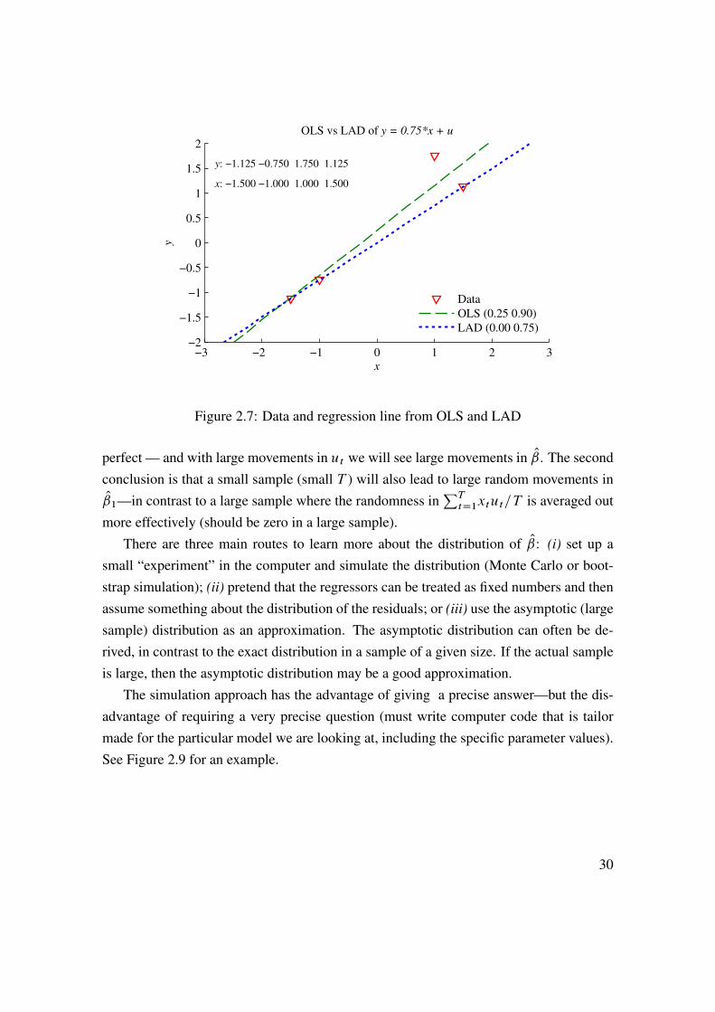
Figure 2.7: Data and regression line from OLS and LAD
perfect — and with large movements in ut we will see large movements in O. The secondconclusion is that a small sample (small T ) will also lead to large random movements inO1—in contrast to a large sample where the randomness in
PTtD1xtut=T is averaged out
more effectively (should be zero in a large sample).There are three main routes to learn more about the distribution of O: (i) set up a
small “experiment” in the computer and simulate the distribution (Monte Carlo or boot-strap simulation); (ii) pretend that the regressors can be treated as fixed numbers and thenassume something about the distribution of the residuals; or (iii) use the asymptotic (largesample) distribution as an approximation. The asymptotic distribution can often be de-rived, in contrast to the exact distribution in a sample of a given size. If the actual sampleis large, then the asymptotic distribution may be a good approximation.
The simulation approach has the advantage of giving a precise answer—but the dis-advantage of requiring a very precise question (must write computer code that is tailormade for the particular model we are looking at, including the specific parameter values).See Figure 2.9 for an example.
30
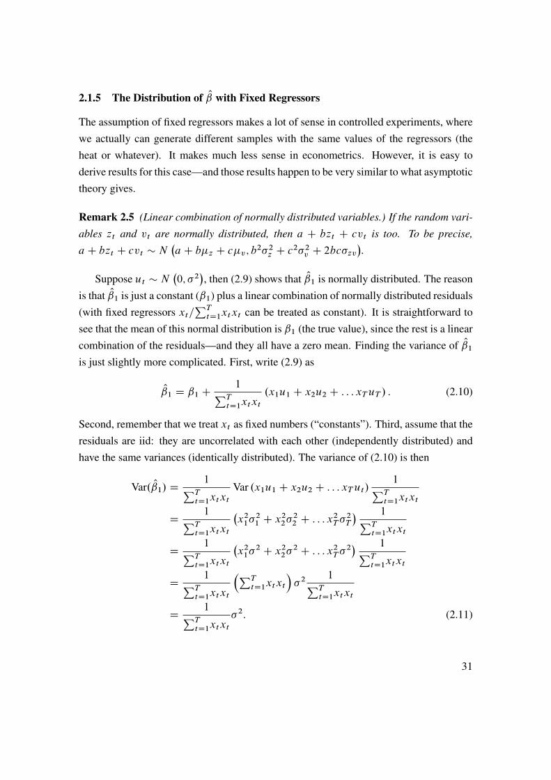
2.1.5 The Distribution of O with Fixed Regressors
The assumption of fixed regressors makes a lot of sense in controlled experiments, wherewe actually can generate different samples with the same values of the regressors (theheat or whatever). It makes much less sense in econometrics. However, it is easy toderive results for this case—and those results happen to be very similar to what asymptotictheory gives.
Remark 2.5 (Linear combination of normally distributed variables.) If the random vari-
ables zt and vt are normally distributed, then a C bzt C cvt is too. To be precise,
aC bzt C cvt � N�aC b�z C c�v; b2�2z C c2�2v C 2bc�zv
�.
Suppose ut � N�0; �2
�, then (2.9) shows that O1 is normally distributed. The reason
is that O1 is just a constant (ˇ1) plus a linear combination of normally distributed residuals(with fixed regressors xt=
PTtD1xtxt can be treated as constant). It is straightforward to
see that the mean of this normal distribution is ˇ1 (the true value), since the rest is a linearcombination of the residuals—and they all have a zero mean. Finding the variance of O1is just slightly more complicated. First, write (2.9) as
O1 D ˇ1 C 1PT
tD1xtxt.x1u1 C x2u2 C : : : xTuT / : (2.10)
Second, remember that we treat xt as fixed numbers (“constants”). Third, assume that theresiduals are iid: they are uncorrelated with each other (independently distributed) andhave the same variances (identically distributed). The variance of (2.10) is then
Var. O1/ D 1PTtD1xtxt
Var .x1u1 C x2u2 C : : : xTut/ 1PTtD1xtxt
D 1PTtD1xtxt
�x21�
21 C x22�22 C : : : x2T �2T
� 1PTtD1xtxt
D 1PTtD1xtxt
�x21�
2 C x22�2 C : : : x2T �2� 1PT
tD1xtxt
D 1PTtD1xtxt
�PTtD1xtxt
��2
1PTtD1xtxt
D 1PTtD1xtxt
�2: (2.11)
31
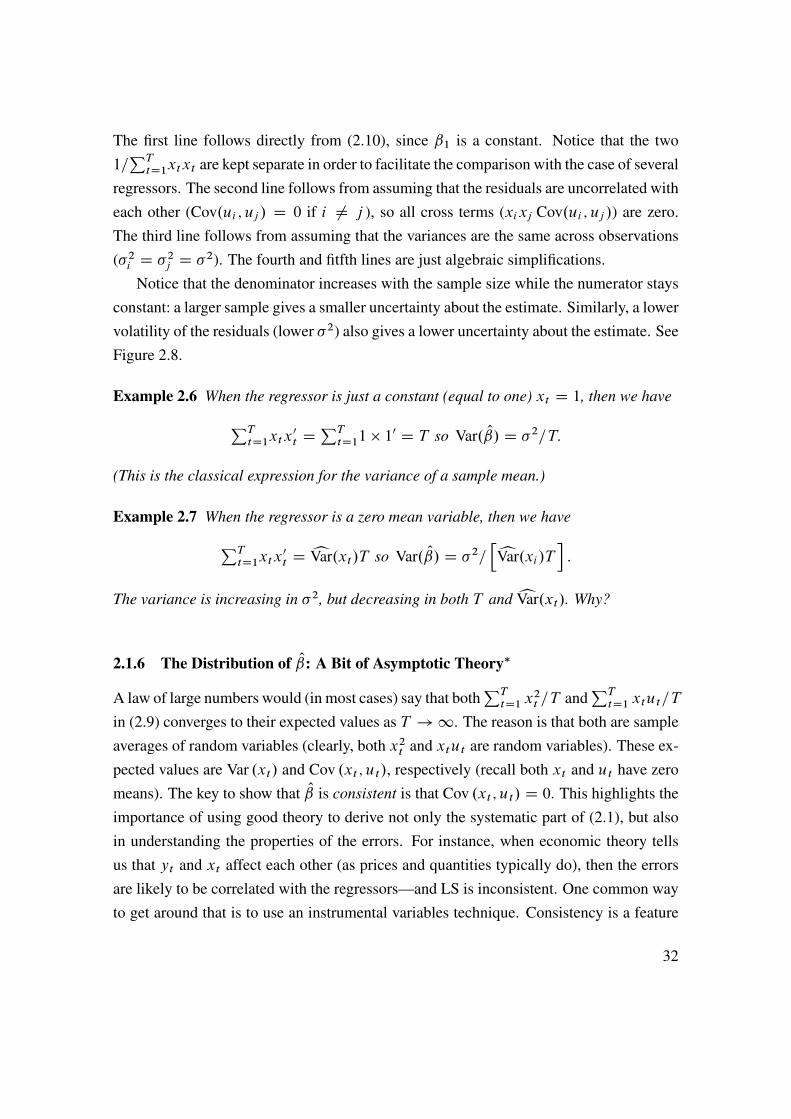
The first line follows directly from (2.10), since ˇ1 is a constant. Notice that the two1=PT
tD1xtxt are kept separate in order to facilitate the comparison with the case of severalregressors. The second line follows from assuming that the residuals are uncorrelated witheach other (Cov.ui ; uj / D 0 if i ¤ j ), so all cross terms (xixj Cov.ui ; uj /) are zero.The third line follows from assuming that the variances are the same across observations(�2i D �2j D �2). The fourth and fitfth lines are just algebraic simplifications.
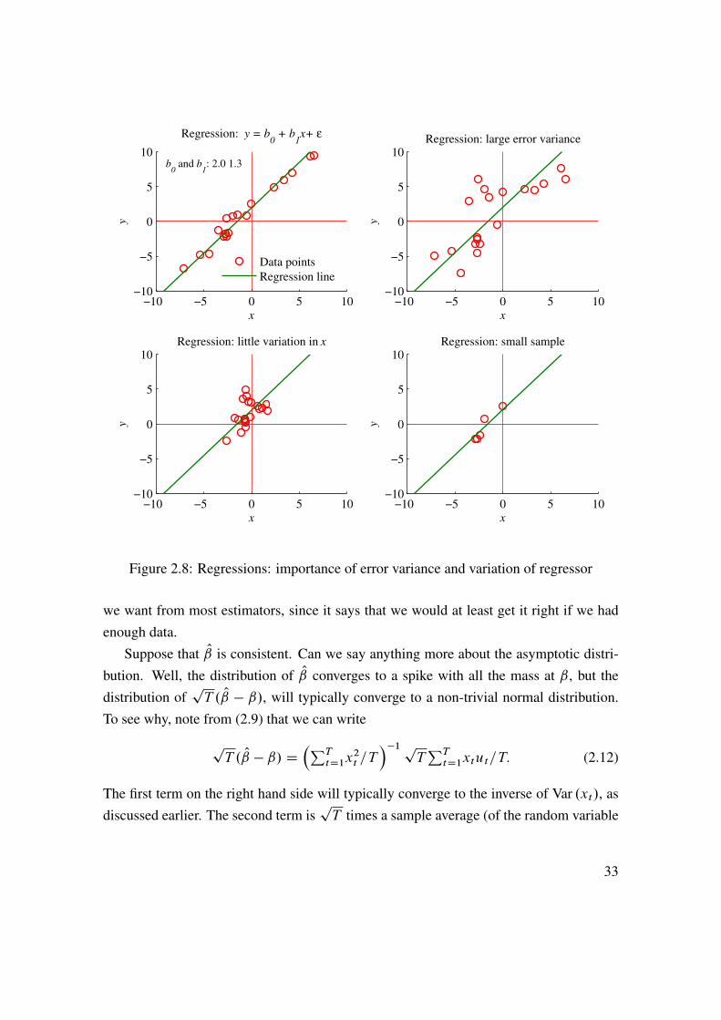
Notice that the denominator increases with the sample size while the numerator staysconstant: a larger sample gives a smaller uncertainty about the estimate. Similarly, a lowervolatility of the residuals (lower �2) also gives a lower uncertainty about the estimate. SeeFigure 2.8.
Example 2.6 When the regressor is just a constant (equal to one) xt D 1, then we havePTtD1xtx
0t D
PTtD11 � 10 D T so Var. O/ D �2=T:
(This is the classical expression for the variance of a sample mean.)
Example 2.7 When the regressor is a zero mean variable, then we havePTtD1xtx
0t D cVar.xt/T so Var. O/ D �2=
hcVar.xi/Ti:
The variance is increasing in �2, but decreasing in both T and cVar.xt/. Why?
2.1.6 The Distribution of O: A Bit of Asymptotic Theory�
A law of large numbers would (in most cases) say that bothPT
tD1 x2t =T and
PTtD1 xtut=T
in (2.9) converges to their expected values as T !1. The reason is that both are sampleaverages of random variables (clearly, both x2t and xtut are random variables). These ex-pected values are Var .xt/ and Cov .xt ; ut/, respectively (recall both xt and ut have zeromeans). The key to show that O is consistent is that Cov .xt ; ut/ D 0. This highlights theimportance of using good theory to derive not only the systematic part of (2.1), but alsoin understanding the properties of the errors. For instance, when economic theory tellsus that yt and xt affect each other (as prices and quantities typically do), then the errorsare likely to be correlated with the regressors—and LS is inconsistent. One common wayto get around that is to use an instrumental variables technique. Consistency is a feature
32
−10 −5 0 5 10−10
−5
0
5
10
Regression: y = b0 + b
1x+ ε
x
y
b
0 and b
1: 2.0 1.3
Data points
Regression line
−10 −5 0 5 10−10
−5
0
5
10Regression: large error variance
x
y
−10 −5 0 5 10−10
−5
0
5
10Regression: little variation in x
x
y
−10 −5 0 5 10−10
−5
0
5
10Regression: small sample
x
y
Figure 2.8: Regressions: importance of error variance and variation of regressor
we want from most estimators, since it says that we would at least get it right if we hadenough data.
Suppose that O is consistent. Can we say anything more about the asymptotic distri-bution. Well, the distribution of O converges to a spike with all the mass at ˇ, but thedistribution of
pT . O � ˇ/, will typically converge to a non-trivial normal distribution.
To see why, note from (2.9) that we can write
pT . O � ˇ/ D
�PTtD1x
2t =T
��1pTPT
tD1xtut=T: (2.12)
The first term on the right hand side will typically converge to the inverse of Var .xt/, asdiscussed earlier. The second term is
pT times a sample average (of the random variable
33

−4 −2 0 2 40
0.1
0.2
0.3
0.4
Distribution of t−stat, T=5
−4 −2 0 2 40
0.1
0.2
0.3
0.4
Distribution of t−stat, T=100
Model: Rt=0.9f
t+ε
t, ε
t = v
t − 2 where v
t has a χ
2(2) distribution
Results for T=5 and T=100:
Kurtosis of t−stat: 71.9 3.1
Frequency of abs(t−stat)>1.645: 0.25 0.10
Frequency of abs(t−stat)>1.96: 0.19 0.06
−4 −2 0 2 40
0.1
0.2
0.3
0.4
Probability density functions
N(0,1)
χ2(2)−2
Figure 2.9: Distribution of LS estimator when residuals have a non-normal distribution
xtut ) with a zero expected value, since we assumed that O is consistent. Under weakconditions, a central limit theorem applies so
pT times a sample average converges to a
normal distribution. This shows thatpT O has an asymptotic normal distribution. It turns
out that this is a property of many estimators, basically because most estimators are somekind of sample average. The properties of this distribution are quite similar to those thatwe derived by assuming that the regressors were fixed numbers.
2.1.7 Multiple Regression
All the previous results still hold in a multiple regression—with suitable reinterpretationsof the notation.
34

Consider the linear model
yt D x1tˇ1 C x2tˇ2 C � � � C xktˇk C utD x0tˇ C ut ; (2.13)
where yt and ut are scalars, xt a k�1 vector, and ˇ is a k�1 vector of the true coefficients(see Appendix A for a summary of matrix algebra). Least squares minimizes the sum ofthe squared fitted residuals PT
tD1 Ou2t DPT
tD1.yt � x0t O/2; (2.14)
by choosing the vector ˇ. The first order conditions are
0kx1 DPT
tD1xt.yt � x0t O/ orPT
tD1xtyt DPT
tD1xtx0tO; (2.15)
which can be solved asO D
�PTtD1xtx
0t
��1PTtD1xtyt : (2.16)
Example 2.8 With 2 regressors (k D 2), (2.15) is"0
0
#DPT
tD1
"x1t.yt � x1t O1 � x2t O2/x2t.yt � x1t O1 � x2t O2/
#
and (2.16) is " O1
O2
#D PT
tD1
"x1tx1t x1tx2t
x2tx1t x2tx2t
#!�1PTtD1
"x1tyt
x2tyt
#:
2.2 Hypothesis Testing
2.2.1 Testing a Single Coefficient
We assume that the estimates are normally distributed. To be able to easily compare withprinted tables of probabilities, we transform to a N.0; 1/ variable as
t DO � ˇ
Std. O/� N.0; 1/; (2.17)
where Std. O/ is the standard error (deviation) of O.
35
The logic of a hypothesis test is perhaps best described by a example. Suppose youwant to test the hypothesis that ˇ D 1. (Econometric programs often automatically reportresults for the null hypothesis that ˇ D 0.) The steps are then as follows.
1. Construct distribution under H0: set ˇ D 1 in (2.17).
2. Would test statistic (t ) you get be very unusual under theH0 distribution? Dependson the alternative and what tolerance you have towards unusual outcomes.
3. What is the alternative hypothesis? Suppose H1: ˇ ¤ 1 so unusual is the same asa value of O far from 1, that is, jt j is large.
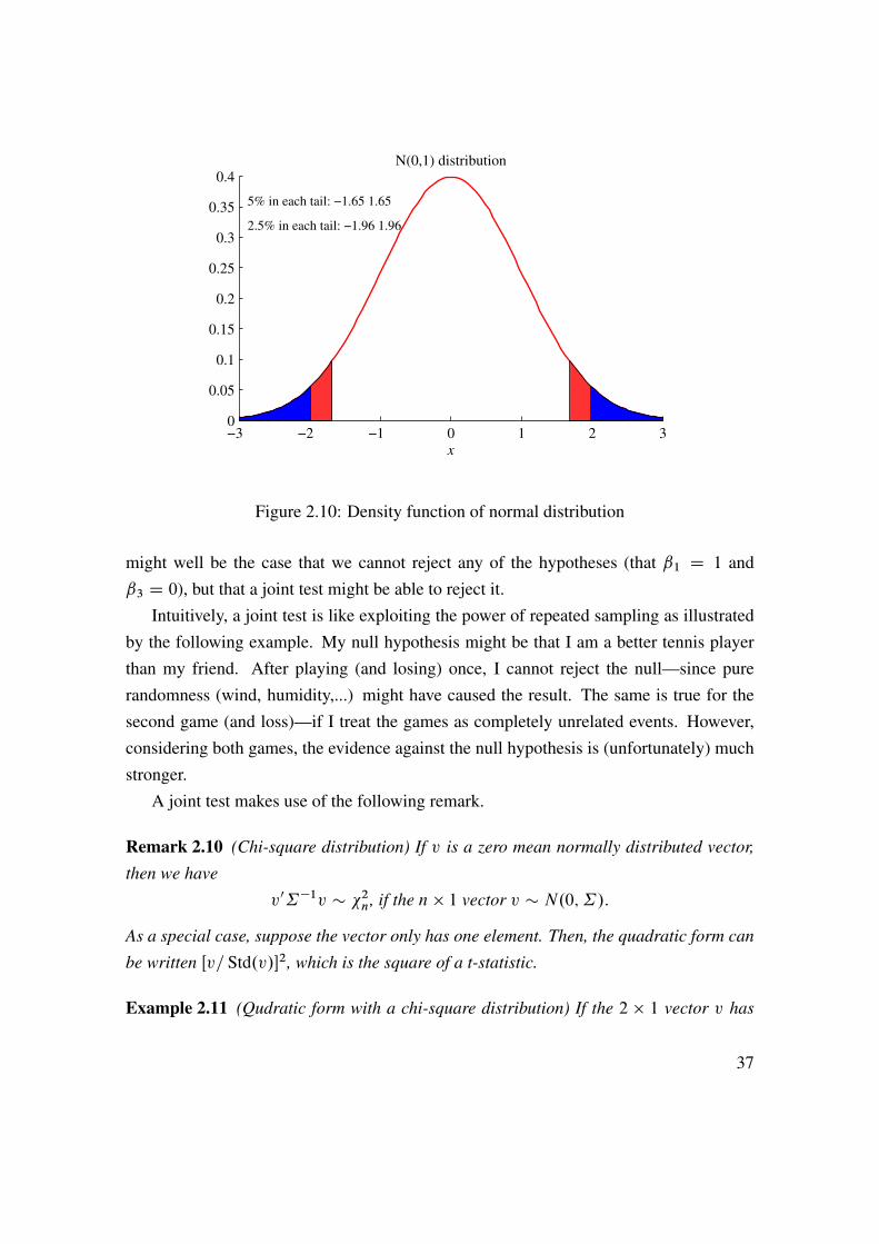
4. Define how tolerant towards unusual outcomes you are. For instance, choose acutoff value so that the test statistic beyond this would happen less than 10% (sig-nificance level) of the times in case your H0 was actually true. Since two-sidedtest: use both tails, so the critical values are (�1:65 and 1:65). See Figure 2.10 foran example. The idea that values beyond (�1:65 and 1:65) are unlikely to happenif your H0 is true, so if you get such a t -stat, then your H0 is probably false: youreject it. See Tables 2.1 and Table 2.2 for examples.
Clearly, a 5% significance level gives the critical values �1:96 and 1:96,which wouldbe really unusual under H0. We sometimes compare with a t -distribution instead ofa N.0; 1/, especially when the sample is short. For samples of more than 30–40 datapoints, the difference is trivial—see Table A.1. The p-value is a related concept. It is thelowest significance level at which we can reject the null hypothesis.
Example 2.9 Std. O/ D 1:5, O D 3 and ˇ D 1 (underH0): t D .3�1/=1:5 � 1:33 so we
cannot rejectH0 at the 10% significance level. Instead, if O D 4, then t D .4� 1/=1:5 D2, so we could reject the null hypothesis.
2.2.2 Joint Test of Several Coefficients
A joint test of several coefficients is different from testing the coefficients one at a time.For instance, suppose your economic hypothesis is that ˇ1 D 1 and ˇ3 D 0. You couldclearly test each coefficient individually (by a t-test), but that may give conflicting results.In addition, it does not use the information in the sample as effectively as possible. It
36
−3 −2 −1 0 1 2 30
0.05
0.1
0.15
0.2
0.25
0.3
0.35
0.4
N(0,1) distribution
x
5% in each tail: −1.65 1.65
2.5% in each tail: −1.96 1.96
Figure 2.10: Density function of normal distribution
might well be the case that we cannot reject any of the hypotheses (that ˇ1 D 1 andˇ3 D 0), but that a joint test might be able to reject it.
Intuitively, a joint test is like exploiting the power of repeated sampling as illustratedby the following example. My null hypothesis might be that I am a better tennis playerthan my friend. After playing (and losing) once, I cannot reject the null—since purerandomness (wind, humidity,...) might have caused the result. The same is true for thesecond game (and loss)—if I treat the games as completely unrelated events. However,considering both games, the evidence against the null hypothesis is (unfortunately) muchstronger.
A joint test makes use of the following remark.
Remark 2.10 (Chi-square distribution) If v is a zero mean normally distributed vector,
then we have
v0˙�1v � �2n, if the n � 1 vector v � N.0;˙/:As a special case, suppose the vector only has one element. Then, the quadratic form can
be written Œv=Std.v/�2, which is the square of a t-statistic.
Example 2.11 (Qudratic form with a chi-square distribution) If the 2 � 1 vector v has
37

0 5 10 150
0.5
1
χ2
1 distribution
x
Pr(x ≥ : 2.71) is 0.1
0 5 10 150
0.1
0.2
0.3
0.4
χ2
2 distribution
x
Pr(x ≥ : 4.61) is 0.1
0 5 10 150
0.05
0.1
0.15
χ2
5 distribution
x
Pr(x ≥ : 9.24) is 0.1
Figure 2.11: Density functions of �2 distributions with different degrees of freedom
the following nornal distribution"v1
v2
#� N
"0
0
#;
"1 0
0 2
#!;
then the quadratic form "v1
v2
#0 "1 0
0 1=2
#"v1
v2
#D v21 C v22=2
has a �22 distribution.
For instance, suppose we have estimated a model with three coefficients and the nullhypothesis is
H0 W ˇ1 D 1 and ˇ3 D 0: (2.18)
38
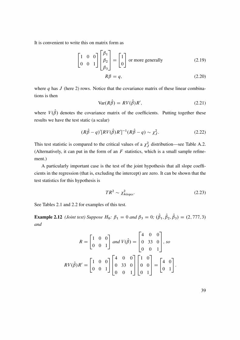
It is convenient to write this on matrix form as
"1 0 0
0 0 1
#264ˇ1ˇ2ˇ3
375 D "10
#or more generally (2.19)
Rˇ D q; (2.20)
where q has J (here 2) rows. Notice that the covariance matrix of these linear combina-tions is then
Var.R O/ D RV. O/R0; (2.21)
where V. O/ denotes the covariance matrix of the coefficients. Putting together theseresults we have the test static (a scalar)
.R O � q/0ŒRV. O/R0��1.R O � q/ � �2J : (2.22)
This test statistic is compared to the critical values of a �2J distribution—see Table A.2.(Alternatively, it can put in the form of an F statistics, which is a small sample refine-ment.)
A particularly important case is the test of the joint hypothesis that all slope coeffi-cients in the regression (that is, excluding the intercept) are zero. It can be shown that thetest statistics for this hypothesis is
TR2 � �2#slopes: (2.23)
See Tables 2.1 and 2.2 for examples of this test.
Example 2.12 (Joint test) Suppose H0: ˇ1 D 0 and ˇ3 D 0; . O1; O2; O3/ D .2; 777; 3/
and
R D"1 0 0
0 0 1
#and V. O/ D
2644 0 0
0 33 0
0 0 1
375 , so
RV. O/R0 D"1 0 0
0 0 1
#2644 0 0
0 33 0
0 0 1
3752641 0
0 0
0 1
375 D "4 0
0 1
#:
39

Then, (2.22) is0B@"1 0 0
0 0 1
#264 2
777
3
375 � "00
#1CA0 "4 0
0 1
#�10B@"1 0 0
0 0 1
#264 2
777
3
375 � "00
#1CAh2 3
i "0:25 0
0 1
#"2
3
#D 10;
which is higher than the 10% critical value of the �22 distribution (which is 4.61).
2.3 Heteroskedasticity
Suppose we have a regression model
yt D x0tb C ut ; where Eut D 0 and Cov.xit ; ut/ D 0: (2.24)
In the standard case we assume that ut is iid (independently and identically distributed),which rules out heteroskedasticity.
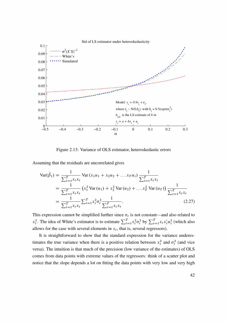
In case the residuals actually are heteroskedastic, least squares (LS) is nevertheless auseful estimator: it is still consistent (we get the correct values as the sample becomesreally large)—and it is reasonably efficient (in terms of the variance of the estimates).However, the standard expression for the standard errors (of the coefficients) is (except ina special case, see below) not correct. This is illustrated in Figure 2.13.
To test for heteroskedasticity, we can use White’s test of heteroskedasticity. The nullhypothesis is homoskedasticity, and the alternative hypothesis is the kind of heteroskedas-ticity which can be explained by the levels, squares, and cross products of the regressors—clearly a special form of heteroskedasticity. The reason for this specification is that if thesquared residual is uncorrelated with these squared regressors, then the usual LS covari-ance matrix applies—even if the residuals have some other sort of heteroskedasticity (thisis the special case mentioned before).
To implement White’s test, let wi be the squares and cross products of the regressors.The test is then to run a regression of squared fitted residuals on wt
Ou2t D w0t C vt ; (2.25)
40
−10 −5 0 5 10
−20
−10
0
10
20
Scatter plot, iid residuals
x
y
−10 −5 0 5 10
−20
−10
0
10
20
Scatter plot, Var(residual) depends on x2
x
y
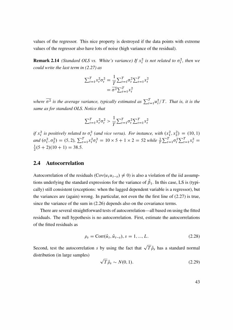
y = 0.03 + 1.3x + u
Solid regression lines are based on all data, dashed lines exclude the crossed out data point
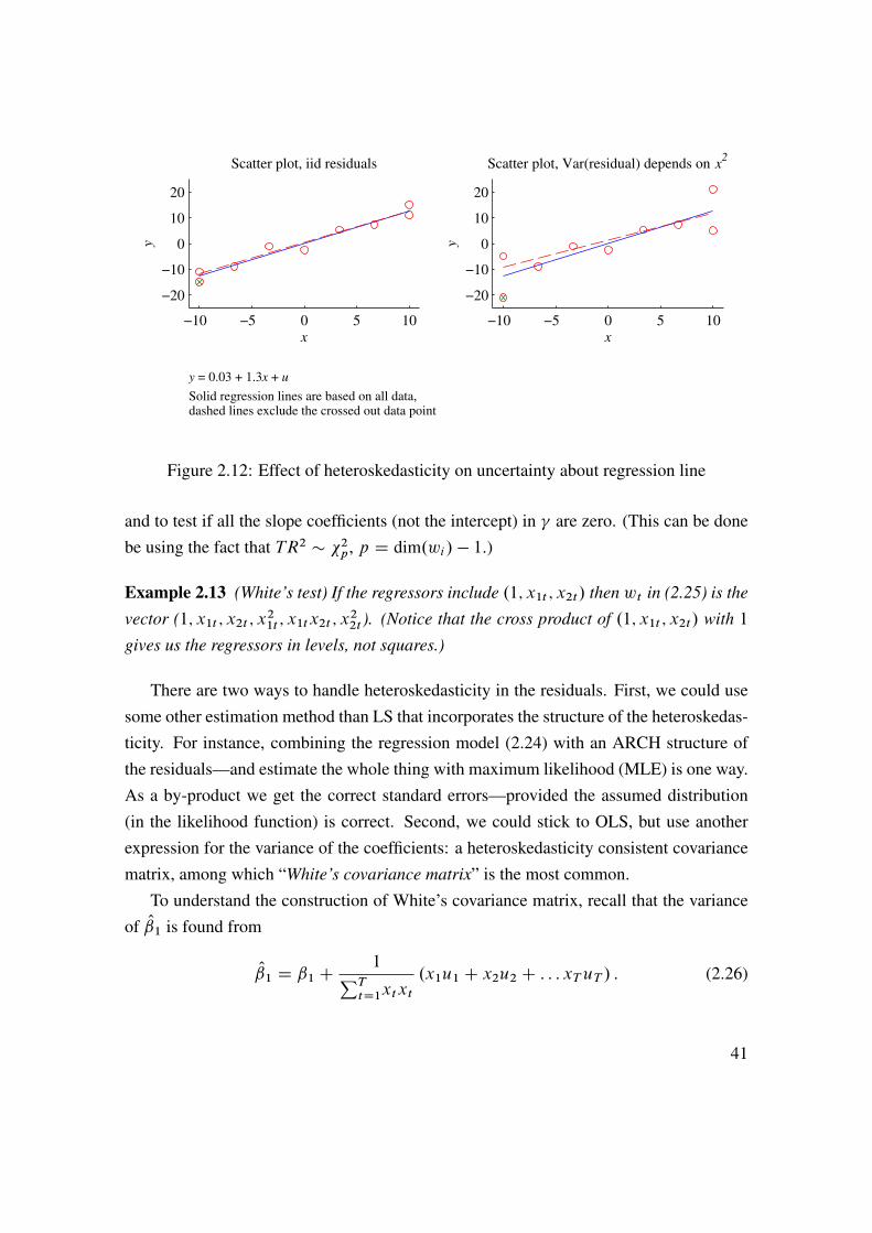
Figure 2.12: Effect of heteroskedasticity on uncertainty about regression line
and to test if all the slope coefficients (not the intercept) in are zero. (This can be donebe using the fact that TR2 � �2p, p D dim.wi/ � 1:)
Example 2.13 (White’s test) If the regressors include .1; x1t ; x2t/ then wt in (2.25) is the
vector (1; x1t ; x2t ; x21t ; x1tx2t ; x22t ). (Notice that the cross product of .1; x1t ; x2t/ with 1
gives us the regressors in levels, not squares.)
There are two ways to handle heteroskedasticity in the residuals. First, we could usesome other estimation method than LS that incorporates the structure of the heteroskedas-ticity. For instance, combining the regression model (2.24) with an ARCH structure ofthe residuals—and estimate the whole thing with maximum likelihood (MLE) is one way.As a by-product we get the correct standard errors—provided the assumed distribution(in the likelihood function) is correct. Second, we could stick to OLS, but use anotherexpression for the variance of the coefficients: a heteroskedasticity consistent covariancematrix, among which “White’s covariance matrix” is the most common.
To understand the construction of White’s covariance matrix, recall that the varianceof O1 is found from
O1 D ˇ1 C 1PT
tD1xtxt.x1u1 C x2u2 C : : : xTuT / : (2.26)
41
−0.5 −0.4 −0.3 −0.2 −0.1 0 0.1 0.2 0.30
0.01
0.02
0.03
0.04
0.05
0.06
0.07
0.08
0.09
0.1Std of LS estimator under heteroskedasticity
α
Model: yt = 0.9x
t + ε
t,
where εt ∼ N(0,h
t), with h
t = 0.5exp(αx
t
2)
bLS
is the LS estimate of b in
yt = a + bx
t + u
t
σ2(X’X)
−1
White’s
Simulated
Figure 2.13: Variance of OLS estimator, heteroskedastic errors
Assuming that the residuals are uncorrelated gives
Var. O1/ D 1PTtD1xtxt
Var .x1u1 C x2u2 C : : : xTut/ 1PTtD1xtxt
D 1PTtD1xtxt
�x21 Var .u1/C x22 Var .u2/C : : : x2T Var .uT /
� 1PTtD1xtxt
D 1PTtD1xtxt
PTtD1x
2t �
2t
1PTtD1xtxt
: (2.27)
This expression cannot be simplified further since �t is not constant—and also related tox2t . The idea of White’s estimator is to estimate
PTtD1x
2t �
2t by
PTtD1xtx
0tu2t (which also
allows for the case with several elements in xt , that is, several regressors).It is straightforward to show that the standard expression for the variance underes-
timates the true variance when there is a positive relation between x2t and �2t (and viceversa). The intuition is that much of the precision (low variance of the estimates) of OLScomes from data points with extreme values of the regressors: think of a scatter plot andnotice that the slope depends a lot on fitting the data points with very low and very high
42
values of the regressor. This nice property is destroyed if the data points with extremevalues of the regressor also have lots of noise (high variance of the residual).
Remark 2.14 (Standard OLS vs. White’s variance) If x2t is not related to �2t , then we
could write the last term in (2.27) as
PTtD1x
2t �
2t D
1
T
PTtD1�
2t
PTtD1x
2t
D �2PTtD1x
2t
where �2 is the average variance, typically estimated asPT
tD1u2t =T . That is, it is the
same as for standard OLS. Notice that
PTtD1x
2t �
2t >
1
T
PTtD1�
2t
PTtD1x
2t
if x2t is positively related to �2t (and vice versa). For instance, with .x21 ; x22/ D .10; 1/
and .�21 ; �22 / D .5; 2/,
PTtD1x
2t �
2t D 10 � 5C 1 � 2 D 52 while 1
T
PTtD1�
2t
PTtD1x
2t D
12.5C 2/.10C 1/ D 38:5:
2.4 Autocorrelation
Autocorrelation of the residuals (Cov.utut�s/ ¤ 0) is also a violation of the iid assump-tions underlying the standard expressions for the variance of O1. In this case, LS is (typi-cally) still consistent (exceptions: when the lagged dependent variable is a regressor), butthe variances are (again) wrong. In particular, not even the the first line of (2.27) is true,since the variance of the sum in (2.26) depends also on the covariance terms.
There are several straightforward tests of autocorrelation—all based on using the fittedresiduals. The null hypothesis is no autocorrelation. First, estimate the autocorrelationsof the fitted residuals as
�s D Corr. Out ; Out�s/, s D 1; :::; L: (2.28)
Second, test the autocorrelation s by using the fact thatpT O�s has a standard normal
distribution (in large samples) pT O�s � N.0; 1/: (2.29)
43
−10 −5 0 5 10
−20
0
20
Scatter plot, iid residuals
x
y
−10 −5 0 5 10
−20
0
20
Scatter plot, autocorrelated residuals
x
y
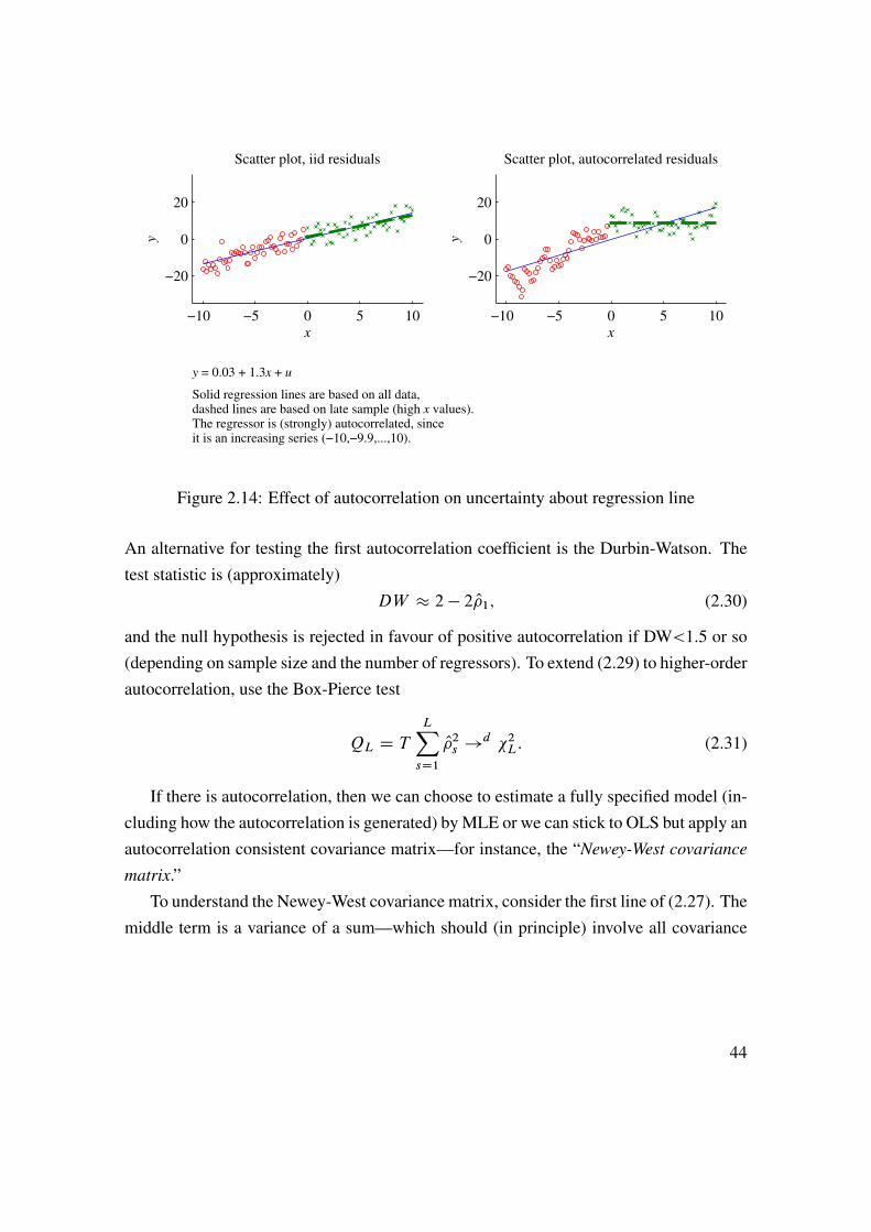
y = 0.03 + 1.3x + u
Solid regression lines are based on all data, dashed lines are based on late sample (high x values).The regressor is (strongly) autocorrelated, since it is an increasing series (−10,−9.9,...,10).
Figure 2.14: Effect of autocorrelation on uncertainty about regression line
An alternative for testing the first autocorrelation coefficient is the Durbin-Watson. Thetest statistic is (approximately)
DW � 2 � 2 O�1; (2.30)
and the null hypothesis is rejected in favour of positive autocorrelation if DW<1.5 or so(depending on sample size and the number of regressors). To extend (2.29) to higher-orderautocorrelation, use the Box-Pierce test
QL D TLXsD1
O�2s !d �2L: (2.31)
If there is autocorrelation, then we can choose to estimate a fully specified model (in-cluding how the autocorrelation is generated) by MLE or we can stick to OLS but apply anautocorrelation consistent covariance matrix—for instance, the “Newey-West covariance
matrix.”To understand the Newey-West covariance matrix, consider the first line of (2.27). The
middle term is a variance of a sum—which should (in principle) involve all covariance
44
−0.5 0 0.5
−0.5
0
0.5
Autocorrelation of xtu
t
ρ
κ = −0.9
κ = 0
κ = 0.9
Model: yt = 0.9x
t + ε
t,
where εt = ρε
t−1 + u
t,
where ut is iid N(0,h) such that Std(ε
t) = 1, and
xt = κx
t−1 + η
t
bLS
is the LS estimate of b in
yt = a + bx
t + u
t
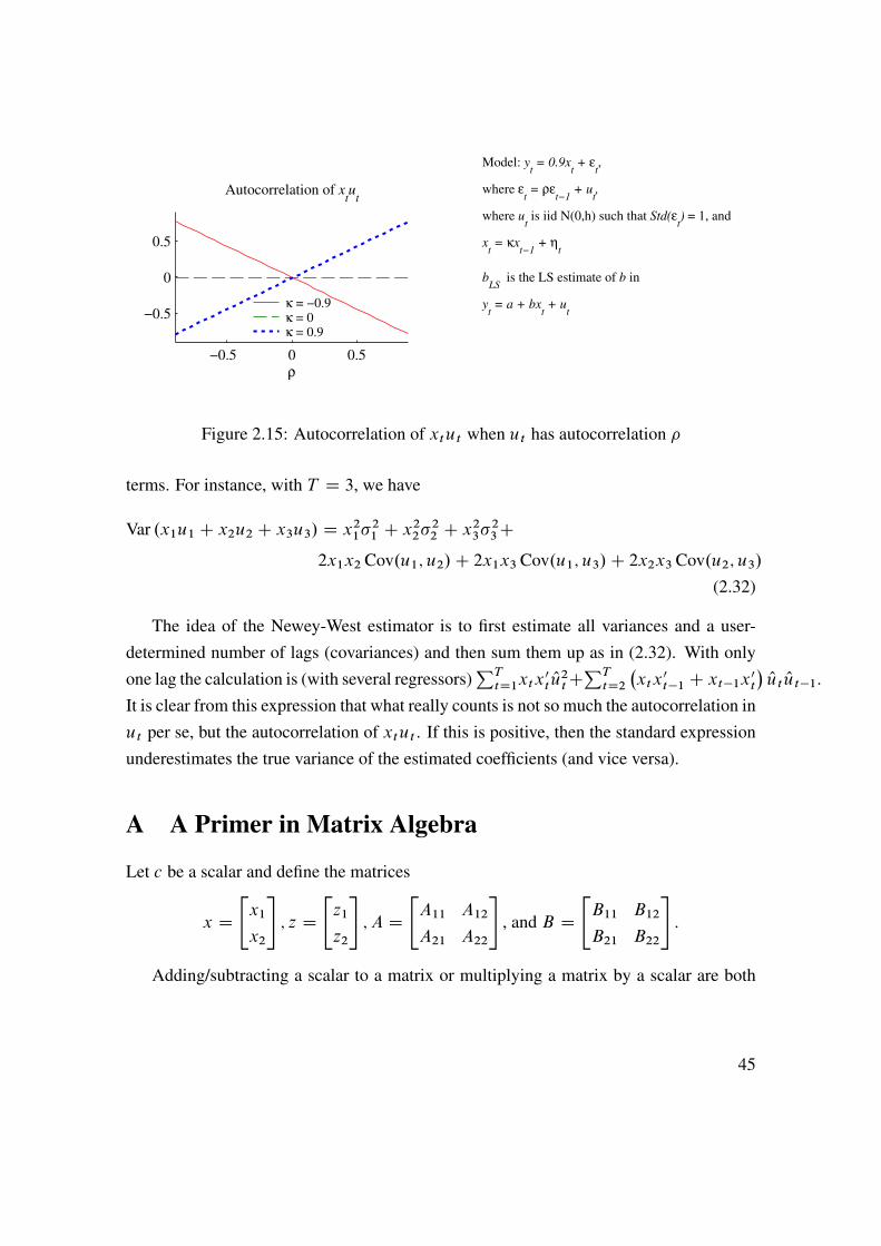
Figure 2.15: Autocorrelation of xtut when ut has autocorrelation �
terms. For instance, with T D 3, we have
Var .x1u1 C x2u2 C x3u3/ D x21�21 C x22�22 C x23�23C2x1x2 Cov.u1; u2/C 2x1x3 Cov.u1; u3/C 2x2x3 Cov.u2; u3/
(2.32)
The idea of the Newey-West estimator is to first estimate all variances and a user-determined number of lags (covariances) and then sum them up as in (2.32). With onlyone lag the calculation is (with several regressors)
PTtD1xtx
0t Ou2tC
PTtD2
�xtx0t�1 C xt�1x0t
� Out Out�1.It is clear from this expression that what really counts is not so much the autocorrelation inut per se, but the autocorrelation of xtut . If this is positive, then the standard expressionunderestimates the true variance of the estimated coefficients (and vice versa).
A A Primer in Matrix Algebra
Let c be a scalar and define the matrices
x D"x1
x2
#; z D
"z1
z2
#; A D
"A11 A12
A21 A22
#, and B D
"B11 B12
B21 B22
#:
Adding/subtracting a scalar to a matrix or multiplying a matrix by a scalar are both
45
−0.5 0 0.50
0.05
0.1
Std of LS under autocorrelation, κ = −0.9
ρ
σ2(X’X)
−1
Newey−West Simulated
−0.5 0 0.50
0.05
0.1
Std of LS under autocorrelation, κ = 0
ρ
−0.5 0 0.50
0.05
0.1
Std of LS under autocorrelation, κ = 0.9
ρ
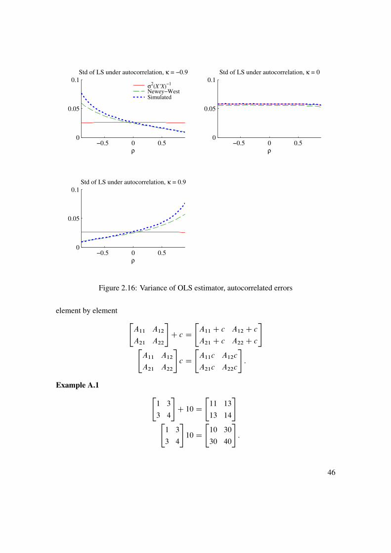
Figure 2.16: Variance of OLS estimator, autocorrelated errors
element by element "A11 A12
A21 A22
#C c D
"A11 C c A12 C cA21 C c A22 C c
#"A11 A12
A21 A22
#c D
"A11c A12c
A21c A22c
#:
Example A.1 "1 3
3 4
#C 10 D
"11 13
13 14
#"1 3
3 4
#10 D
"10 30
30 40
#:
46

0 10 20 30 40 50 60−0.5
0
0.5Return = a + b*lagged Return, slope
Return horizon (months)
Slope with two different 90% conf band, OLS and NW std
US stock returns 1926:1−2010:4, overlapping data
Figure 2.17: Slope coefficient, LS vs Newey-West standard errors
Matrix addition (or subtraction) is element by element
AC B D"A11 A12
A21 A22
#C"B11 B12
B21 B22
#D"A11 C B11 A12 C B12A21 C B21 A22 C B22
#:
Example A.2 (Matrix addition and subtraction/"10
11
#�"2
5
#D"8
6
#"1 3
3 4
#C"1 2
3 �2
#D"2 5
6 2
#To turn a column into a row vector, use the transpose operator like in x0
x0 D"x1
x2
#0Dhx1 x2
i:
Similarly, transposing a matrix is like flipping it around the main diagonal
A0 D"A11 A12
A21 A22
#0D"A11 A21
A12 A22
#:
47
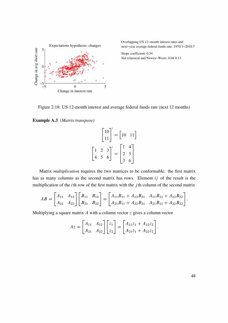
−5 0 5−5
0
5Expectations hypothesis: changes
Change in interest rate
Chan
ge
in a
vg s
hort
rat
e
Overlapping US 12−month interest rates and
next−year average federal funds rate: 1970:1−2010:7
Slope coefficient: 0.54
Std (classical and Newey−West): 0.04 0.13
Figure 2.18: US 12-month interest and average federal funds rate (next 12 months)
Example A.3 (Matrix transpose) "10
11
#0Dh10 11
i"1 2 3
4 5 6
#0D
2641 4
2 5
3 6
375Matrix multiplication requires the two matrices to be conformable: the first matrix
has as many columns as the second matrix has rows. Element ij of the result is themultiplication of the i th row of the first matrix with the j th column of the second matrix
AB D"A11 A12
A21 A22
#"B11 B12
B21 B22
#D"A11B11 C A12B21 A11B12 C A12B22A21B11 C A22B21 A21B12 C A22B22
#:
Multiplying a square matrix A with a column vector z gives a column vector
Az D"A11 A12
A21 A22
#"z1
z2
#D"A11z1 C A12z2A21z1 C A22z2
#:
48

Example A.4 (Matrix multiplication)"1 3
3 4
#"1 2
3 �2
#D"10 �415 �2
#"1 3
3 4
#"2
5
#D"17
26
#
For two column vectors x and z, the product x0z is called the inner product
x0z Dhx1 x2
i "z1z2
#D x1z1 C x2z2;
and xz0 the outer product
xz0 D"x1
x2
# hz1 z2
iD"x1z1 x1z2
x2z1 x2z2
#:
(Notice that xz does not work). If x is a column vector and A a square matrix, then theproduct x0Ax is a quadratic form.
Example A.5 (Inner product, outer product and quadratic form )"10
11
#0 "2
5
#Dh10 11
i "25
#D 75"
10
11
#"2
5
#0D"10
11
# h2 5
iD"20 50
22 55
#"10
11
#0 "1 3
3 4
#"10
11
#D 1244:
A matrix inverse is the closest we get to “dividing” by a matrix. The inverse of amatrix A, denoted A�1, is such that
AA�1 D I and A�1A D I;
where I is the identity matrix (ones along the diagonal, and zeroes elsewhere). The matrixinverse is useful for solving systems of linear equations, y D Ax as x D A�1y.
49

Example A.6 (Matrix inverse) We have"�4=5 3=5
3=5 �1=5
#"1 3
3 4
#D"1 0
0 1
#, so"
1 3
3 4
#�1D"�4=5 3=5
3=5 �1=5
#:
50

A Statistical Tables
n Critical values10% 5% 1%
10 1.81 2.23 3.1720 1.72 2.09 2.8530 1.70 2.04 2.7540 1.68 2.02 2.7050 1.68 2.01 2.6860 1.67 2.00 2.6670 1.67 1.99 2.6580 1.66 1.99 2.6490 1.66 1.99 2.63100 1.66 1.98 2.63Normal 1.64 1.96 2.58
Table A.1: Critical values (two-sided test) of t distribution (different degrees of freedom)and normal distribution.
Bibliography
Verbeek, M., 2008, A guide to modern econometrics, Wiley, Chichester, 3rd edn.
51
n Critical values10% 5% 1%
1 2.71 3.84 6.632 4.61 5.99 9.213 6.25 7.81 11.344 7.78 9.49 13.285 9.24 11.07 15.096 10.64 12.59 16.817 12.02 14.07 18.488 13.36 15.51 20.099 14.68 16.92 21.6710 15.99 18.31 23.21
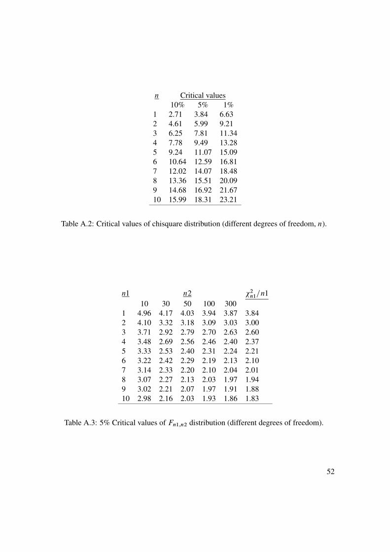
Table A.2: Critical values of chisquare distribution (different degrees of freedom, n).
n1 n2 �2n1=n1
10 30 50 100 3001 4.96 4.17 4.03 3.94 3.87 3.842 4.10 3.32 3.18 3.09 3.03 3.003 3.71 2.92 2.79 2.70 2.63 2.604 3.48 2.69 2.56 2.46 2.40 2.375 3.33 2.53 2.40 2.31 2.24 2.216 3.22 2.42 2.29 2.19 2.13 2.107 3.14 2.33 2.20 2.10 2.04 2.018 3.07 2.27 2.13 2.03 1.97 1.949 3.02 2.21 2.07 1.97 1.91 1.8810 2.98 2.16 2.03 1.93 1.86 1.83
Table A.3: 5% Critical values of Fn1;n2 distribution (different degrees of freedom).
52

n1 n2 �2n1=n1
10 30 50 100 3001 3.29 2.88 2.81 2.76 2.72 2.712 2.92 2.49 2.41 2.36 2.32 2.303 2.73 2.28 2.20 2.14 2.10 2.084 2.61 2.14 2.06 2.00 1.96 1.945 2.52 2.05 1.97 1.91 1.87 1.856 2.46 1.98 1.90 1.83 1.79 1.777 2.41 1.93 1.84 1.78 1.74 1.728 2.38 1.88 1.80 1.73 1.69 1.679 2.35 1.85 1.76 1.69 1.65 1.6310 2.32 1.82 1.73 1.66 1.62 1.60
Table A.4: 10% Critical values of Fn1;n2 distribution (different degrees of freedom).
53

.D..3
3 Index Models
Reference: Elton, Gruber, Brown, and Goetzmann (2010) 7–8, 11
3.1 The Inputs to a MV Analysis
To calculate the mean variance frontier we need to calculate both the expected return andvariance of different portfolios (based on n assets). With two assets (n D 2) the expectedreturn and the variance of the portfolio are
E.Rp/ Dhw1 w2
i "�1�2
#
�2P Dhw1 w2
i "�21 �12
�12 �22
#"w1
w2
#: (3.1)
In this case we need information on 2 mean returns and 3 elements of the covariancematrix. Clearly, the covariance matrix can alternatively be expressed as"
�21 �12
�12 �22
#D"
�21 �12�1�2
�12�1�2 �22
#; (3.2)
which involves two variances and one correlation (3 elements as before).There are two main problems in estimating these parameters: the number of parame-
ters increase very quickly as the number of assets increases and historical estimates haveproved to be somewhat unreliable for future periods.
To illustrate the first problem, notice that with n assets we need the following numberof parameters
Required number of estimates With 100 assets
�i n 100�i i n 100�ij n.n � 1/=2 4950
54
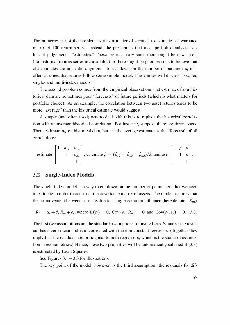
The numerics is not the problem as it is a matter of seconds to estimate a covariancematrix of 100 return series. Instead, the problem is that most portfolio analysis useslots of judgemental “estimates.” These are necessary since there might be new assets(no historical returns series are available) or there might be good reasons to believe thatold estimates are not valid anymore. To cut down on the number of parameters, it isoften assumed that returns follow some simple model. These notes will discuss so-calledsingle- and multi-index models.
The second problem comes from the empirical observations that estimates from his-torical data are sometimes poor “forecasts” of future periods (which is what matters forportfolio choice). As an example, the correlation between two asset returns tends to bemore “average” than the historical estimate would suggest.
A simple (and often used) way to deal with this is to replace the historical correla-tion with an average historical correlation. For instance, suppose there are three assets.Then, estimate �ij on historical data, but use the average estimate as the “forecast” of allcorrelations:
estimate
2641 �12 �13
1 �23
1
375 , calculate N� D . O�12 C O�13 C O�23/=3, and use
2641 N� N�1 N�1
375 :3.2 Single-Index Models
The single-index model is a way to cut down on the number of parameters that we needto estimate in order to construct the covariance matrix of assets. The model assumes thatthe co-movement between assets is due to a single common influence (here denoted Rm)
Ri D ˛iCˇiRmCei , where E.ei/ D 0, Cov .ei ; Rm/ D 0, and Cov.ei ; ej / D 0: (3.3)
The first two assumptions are the standard assumptions for using Least Squares: the resid-ual has a zero mean and is uncorrelated with the non-constant regressor. (Together theyimply that the residuals are orthogonal to both regressors, which is the standard assump-tion in econometrics.) Hence, these two properties will be automatically satisfied if (3.3)is estimated by Least Squares.
See Figures 3.1 – 3.3 for illustrations.The key point of the model, however, is the third assumption: the residuals for dif-
55

−10 −5 0 5 10−10
−8
−6
−4
−2
0
2
4
6
8
10
CAPM regression: Ri−R
f = α
i + β
i×(R
m−R
f)+ e
i
Market excess return,%
Exce
ss r
eturn
ass
et i
,%
Intercept (αi) and slope (β
i): 2.0 1.3
Data points
Regression line
Figure 3.1: CAPM regression
ferent assets are uncorrelated. This means that all comovements of two assets (Ri andRj , say) are due to movements in the common “index” Rm. This is not at all guaranteedby running LS regressions—just an assumption. It is likely to be false—but may be areasonable approximation in many cases. In any case, it simplifies the construction of thecovariance matrix of the assets enormously—as demonstrated below.
Remark 3.1 (The market model) The market model is (3.3) without the assumption that
Cov.ei ; ej / D 0. This model does not simplify the calculation of a portfolio variance—but
will turn out to be important when we want to test CAPM.
If (3.3) is true, then the variance of asset i and the covariance of assets i and j are
�i i D ˇ2i Var .Rm/C Var .ei/ (3.4)
�ij D ˇi j Var .Rm/ : (3.5)
Together, these equations show that we can calculate the whole covariance matrix by
56

−30 −20 −10 0 10 20 30−30
−20
−10
0
10
20
30Scatter plot against market return
Excess return %, market
Exce
ss r
eturn
%, H
iTec
US data 1970:1−2010:9
α
β
−0.14 1.28
−30 −20 −10 0 10 20 30−30
−20
−10
0
10
20
30Scatter plot against market return
Excess return %, market
Exce
ss r
eturn
%, U
tils
α
β
0.22 0.53
Figure 3.2: Scatter plot against market return
having just the variance of the index (to get Var .Rm/) and the output from n regressions(to get ˇi and Var .ei/ for each asset). This is, in many cases, much easier to obtain thandirect estimates of the covariance matrix. For instance, a new asset does not have a returnhistory, but it may be possible to make intelligent guesses about its beta and residualvariance (for instance, from knowing the industry and size of the firm).
This gives the covariance matrix (for two assets)
Cov
"Ri
Rj
#!D"ˇ2i ˇi j
ˇi j ˇ2j
#Var .Rm/C
"Var.ei/ 0
0 Var.ej /
#, or (3.6)
D"ˇi
j
# hˇi j
iVar .Rm/C
"Var.ei/ 0
0 Var.ej /
#(3.7)
More generally, with n assets we can define ˇ to be an n� 1 vector of all the betas and˙to be an n � n matrix with the variances of the residuals along the diagonal. We can thenwrite the covariance matrix of the n � 1 vector of the returns as
Cov.R/ D ˇˇ0Var .Rm/C˙: (3.8)
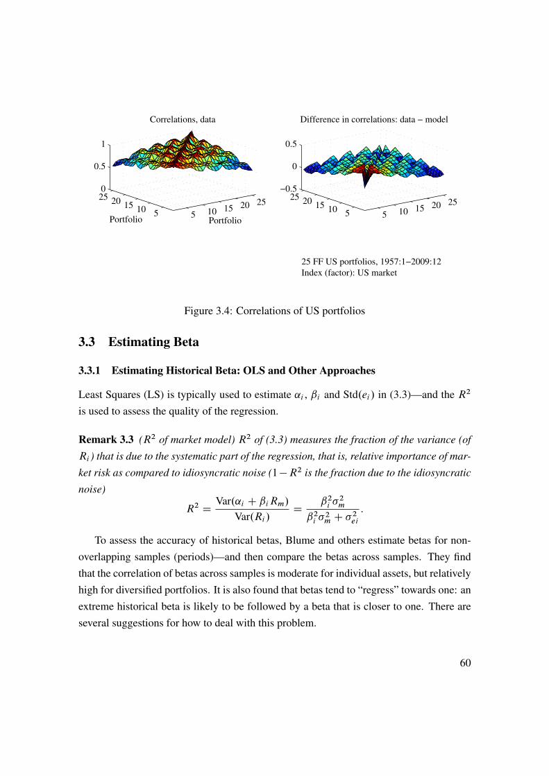
See Figure 3.4 for an example based on the Fama-French portfolios detailed in Table3.2.
Remark 3.2 (Fama-French portfolios) The portfolios in Table 3.2 are calculated by an-
57

HiTec Utils
constant -0.14 0.22(-0.87) (1.42)
market return 1.28 0.53(32.27) (12.55)
R2 0.75 0.35obs 489.00 489.00Autocorr (t) -0.76 0.84White 6.83 19.76All slopes 364.82 170.92
Table 3.1: CAPM regressions, monthly returns, %, US data 1970:1-2010:9. Numbersin parentheses are t-stats. Autocorr is a N(0,1) test statistic (autocorrelation); White is achi-square test statistic (heteroskedasticity), df = K(K+1)/2 - 1; All slopes is a chi-squaretest statistic (of all slope coeffs), df = K-1
nual rebalancing (June/July). The US stock market is divided into 5 � 5 portfolios as
follows. First, split up the stock market into 5 groups based on the book value/market
value: put the lowest 20% in the first group, the next 20% in the second group etc. Sec-
ond, split up the stock market into 5 groups based on size: put the smallest 20% in the first
group etc. Then, form portfolios based on the intersections of these groups. For instance,
in Table 3.2 the portfolio in row 2, column 3 (portfolio 8) belong to the 20%-40% largest
firms and the 40%-60% firms with the highest book value/market value.
Book value/Market value1 2 3 4 5
Size 1 1 2 3 4 52 6 7 8 9 103 11 12 13 14 154 16 17 18 19 205 21 22 23 24 25
Table 3.2: Numbering of the FF indices in the figures.
Proof. (of (3.4)–(3.5) By using (3.3) and recalling that Cov.Rm; ei/ D 0 direct calcu-
58

NoDur Durbl Manuf Enrgy HiTec Telcm Shops Hlth Utils Other0.5
1
1.5
US industry portfolios, β against the market, 1970:1−2010:9β
Figure 3.3: ˇs of US industry portfolios
lations give
�i i D Var .Ri/
D Var .˛i C ˇiRm C ei/D Var .ˇiRm/C Var .ei/C 2 � 0D ˇ2i Var .Rm/C Var .ei/ :
Similarly, the covariance of assets i and j is (recalling also that Cov�ei ; ej
� D 0)
�ij D Cov�Ri ; Rj
�D Cov
�˛i C ˇiRm C ei ; j C jRm C ej
�D ˇi j Var .Rm/C 0D ˇi j Var .Rm/ :
59
5 10 15 20 25
5101520250
0.5
1
Portfolio
Correlations, data
Portfolio5 10 15 20 25
510152025−0.5
0
0.5
Difference in correlations: data − model
25 FF US portfolios, 1957:1−2009:12
Index (factor): US market
Figure 3.4: Correlations of US portfolios
3.3 Estimating Beta
3.3.1 Estimating Historical Beta: OLS and Other Approaches
Least Squares (LS) is typically used to estimate ˛i , ˇi and Std.ei/ in (3.3)—and the R2
is used to assess the quality of the regression.
Remark 3.3 (R2 of market model) R2 of (3.3) measures the fraction of the variance (of
Ri ) that is due to the systematic part of the regression, that is, relative importance of mar-
ket risk as compared to idiosyncratic noise (1�R2 is the fraction due to the idiosyncratic
noise)
R2 D Var.˛i C ˇiRm/Var.Ri/
D ˇ2i �2m
ˇ2i �2m C �2ei
:
To assess the accuracy of historical betas, Blume and others estimate betas for non-overlapping samples (periods)—and then compare the betas across samples. They findthat the correlation of betas across samples is moderate for individual assets, but relativelyhigh for diversified portfolios. It is also found that betas tend to “regress” towards one: anextreme historical beta is likely to be followed by a beta that is closer to one. There areseveral suggestions for how to deal with this problem.
60

To use Blume’s ad-hoc technique, let Oi1 be the estimate of ˇi from an early sample,and Oi2 the estimate from a later sample. Then regress
Oi2 D 0 C 1 Oi1 C �i (3.9)
and use it for forecasting the beta for yet another sample. Blume found . O 0; O 1/ D.0:343; 0:677/ in his sample.
Other authors have suggested averaging the OLS estimate ( Oi1) with some averagebeta. For instance, . Oi1C1/=2 (since the average beta must be unity) or . Oi1C˙n
iD1Oi1=n/=2
(which will typically be similar since ˙niD1Oi1=n is likely to be close to one).
The Bayesian approach is another (more formal) way of adjusting the OLS estimate.It also uses a weighted average of the OLS estimate, Oi1, and some other number, ˇ0,.1 � F / Oi1 C Fˇ0 where F depends on the precision of the OLS estimator. The generalidea of a Bayesian approach (Greene (2003) 16) is to treat both Ri and ˇi as random. Inthis case a Bayesian analysis could go as follows. First, suppose our prior beliefs (beforehaving data) about ˇi is that it is normally distributed,N.ˇ0; �20 /, where (ˇ0; �20 ) are somenumbers . Second, run a LS regression of (3.3). If the residuals are normally distributed,so is the estimator—it is N. Oi1; �2ˇ1/, where we have taken the point estimate to be themean. If we treat the variance of the LS estimator (�2
ˇ1) as known, then the Bayesian
estimator of beta is
b D .1 � F / Oi1 C Fˇ0, where
F D 1=�201=�20 C 1=�2ˇ1
D�2ˇ1
�20 C �2ˇ1: (3.10)
3.3.2 Fundamental Betas
Another way to improve the forecasts of the beta over a future period is to bring in infor-mation about fundamental firm variables. This is particularly useful when there is littlehistorical data on returns (for instance, because the asset was not traded before).
It is often found that betas are related to fundamental variables as follows (with signsin parentheses indicating the effect on the beta): Dividend payout (-), Asset growth (+),Leverage (+), Liquidity (-), Asset size (-), Earning variability (+), Earnings Beta (slope inearnings regressed on economy wide earnings) (+). Such relations can be used to makean educated guess about the beta of an asset without historical data on the returns—but
61
with data on (at least some) of these fundamental variables.
3.4 Multi-Index Models
3.4.1 Overview
The multi-index model is just a multivariate extension of the single-index model (3.3)
Ri D a�i C b�i1I �1 C b�i2I �2 C : : :C b�ikI �k C ei , where (3.11)
E.ei/ D 0, Cov�ei ; I
�k
� D 0, and Cov.ei ; ej / D 0:
As an example, there could be two indices: the stock market return and an interest rate.An ad-hoc approach is to first try a single-index model and then test if the residuals areapproximately uncorrelated. If not, then adding a second index might give an acceptableapproximation.
It is often found that it takes several indices to get a reasonable approximation—butthat a single-index model is equally good (or better) at “forecasting” the covariance overa future period. This is much like the classical trade-off between in-sample fit (requires alarge model) and forecasting (often better with a small model).
The types of indices vary, but one common set captures the “business cycle” andincludes things like the market return, interest rate (or some measure of the yield curveslope), GDP growth, inflation, and so forth. Another common set of indices are industryindices.
It turns out (see below) that the calculations of the covariance matrix are much simplerif the indices are transformed to be uncorrelated so we get the model
Ri D ai C bi1I1 C bi2I2 C : : :C bikIk C ei ; where (3.12)
E.ei/ D 0, Cov�ei ; Ij
� D 0, Cov.ei ; ej / D 0 (unless i D j /, and
Cov.Ij ; Ih/ D 0 (unless j D h).
If this transformation of the indices is linear (and non-singular, so it is can be reversed ifwe want to), then the fit of the regression is unchanged.
62

3.4.2 “Rotating” the Indices
There are several ways of transforming the indices to make them uncorrelated, but the fol-lowing regression approach is perhaps the simplest and may also give the best possibilityof interpreting the results:
1. Let the first transformed index equal the original index, I1 D I �1 (possibly de-meaned). This would often be the market return.
2. Regress the second original index on the first transformed index, I �2 D 0C 1I1C"2. Then, let the second transformed index be the fitted residual, I2 D O"2.
3. Regress the third original index on the first two transformed indices, I �3 D �0 C�1I1 C �2I2 C "3. Then, let I3 D O"3. Follow the same idea for all subsequentindices.
Recall that the fitted residual (from Least Squares) is always uncorrelated with theregressor (by construction). In this case, this means that I2 is uncorrelated with I1 (step2) and that I3 is uncorrelated with both I1 and I2 (step 3). The correlation matrix of thefirst three rotated indices is therefore
Corr
0B@264I1I2I3
3751CA D
2641 0 0
0 1 0
0 0 1
375 : (3.13)
This recursive approach also helps in interpreting the transformed indices. Supposethe first index is the market return and that the second original index is an interest rate.The first transformed index (I1) is then clearly the market return. The second transformedindex (I2) can then be interpreted as the interest rate minus the interest rate expected at thecurrent stock market return—that is, the part of the interest rate that cannot be explainedby the stock market return.
More generally, let the j th index (j D 1; 2; : : : ; k) be
Ij D O"j , where O"j is the fitted residual from the regression (3.14)
I �j D j1 C j1I1 C : : :C j;j�1Ij�1 C "j : (3.15)
Notice that for the first index (j D 1), the regression is only I �1 D 11 C "1, so I1 equalsthe demeaned I �1 .
63

3.4.3 Multi-Index Model after “Rotating” the Indices
To see why the transformed indices are very convenient for calculating the covariancematrix, consider a two-index model. Then, (3.12) implies that the variance of asset i is
�i i D Var .ai C bi1I1 C bi2I2 C ei/D b2i1 Var .I1/C b2i2 Var .I2/C Var .ei/ : (3.16)
Similarly, the covariance of assets i and j is
�ij D Cov�ai C bi1I1 C bi2I2 C ei ; aj C bj1I1 C bj2I2 C ej
�D bi1bj1 Var .I1/C bi2bj2 Var .I2/ : (3.17)
More generally, with n assets and k indices we can define b1 to be an n � 1 vector ofthe slope coefficients for the first index (bi1; bj1) and b2 the vector of slope coefficientsfor the second index and so on. Also, let ˙ to be an n � n matrix with the variances ofthe residuals along the diagonal. The covariance matrix of the returns is then
Cov.R/ D b1b01 Var .I1/C b2b02 Var .I2/C : : :C bkb0k Var .Ik/C˙: (3.18)
See Figure 3.5 for an example.
3.4.4 Multi-Index Model as Method in Portfolio Choice
The factor loadings (betas) can be used for more than just constructing the covariance ma-trix. In fact, the factor loadings are often used directly in portfolio choice. The reason issimple: the betas summarize how different assets are exposed to the big risk factors/returndrivers. The betas therefore provide a way to understand the broad features of even com-plicated portfolios. Combined this with the fact that many analysts and investors havefairly little direct information about individual assets, but are often willing to form opin-ions about the future relative performance of different asset classes (small vs large firms,equity vs bonds, etc)—and the role for factor loadings becomes clear.
See Figures 3.6–3.7 for an illustration.
64

5 10 15 20 25
5101520250
0.5
1
Portfolio
Correlations, data
Portfolio5 10 15 20 25
510152025−0.5
0
0.5
Difference in correlations: data − model
25 FF US portfolios, 1957:1−2009:12
Indices (factors): US market, SMB, HML
Figure 3.5: Correlations of US portfolios
3.5 Principal Component Analysis
Principal component analysis (PCA) can help us determine how many factors that areneeded to explain a cross-section of asset returns.
Let zt D Rt � NRt be an n � 1 vector of demeaned returns with covariance matrix ˙ .The first principal component (pc1t ) is the (normalized) linear combinations of zt thataccount for as much of the variability as possible—and its variance is denoted �1. Thej th (j � 2) principal component (pcjt ) is similar (and its variance is denoted �j ), exceptthat is must be uncorrelated with all lower principal components. Remark 3.4 gives a aformal definition.
Remark 3.4 (Principal component analysis) Consider the zero meanN�1 vector zt with
covariance matrix ˙ . The first (sample) principal component is pc1t D w01zt , where w1is the eigenvector associated with the largest eigenvalue (�1) of ˙ . This value of w1solves the problem maxw w0˙w subject to the normalization w0w D 1. The eigenvalue
�1 equals Var.pc1t/ D w01˙w1. The j th principal component solves the same problem,
but under the additional restriction that w0iwj D 0 for all i < j . The solution is the
eigenvector associated with the j th largest eigenvalue �j (which equals Var.pcjt/ Dw0j˙wj ).
65

0 5 10 15 20 25
1
1.2
1.4
US portfolios, βm
, 1957:1−2009:12
Portfolio
β
0 5 10 15 20 25
0
0.5
1
1.5
US portfolios, βSMBres
Portfolio
β
0 5 10 15 20 25−0.4
−0.2
0
0.2
0.4
0.6
0.8
US portfolios, βHMLres
Portfolio
β
Figure 3.6: Loading (betas) of rotated factors
Let the i th eigenvector be the i th column of the n � n matrix
W D Œ w1 � � � wn �: (3.19)
We can then calculate the n � 1 vector of principal components as
pct D W 0zt : (3.20)
Since the eigenvectors are ortogonal it can be shown that W 0 D W �1, so the expressioncan be inverted as
zt D Wpct : (3.21)
This shows that the i th eigenvector (the i th column of W ) can be interpreted as the effectof the i th principal component on each of the elements in zt . However, the sign of column
66
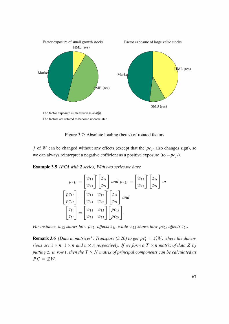
Market
SMB (res)
HML (res)
Factor exposure of small growth stocks
The factor exposure is measured as abs(β)
The factors are rotated to become uncorrelated
Market
SMB (res)
HML (res)
Factor exposure of large value stocks
Figure 3.7: Absolute loading (betas) of rotated factors
j of W can be changed without any effects (except that the pcjt also changes sign), sowe can always reinterpret a negative cofficient as a positive exposure (to �pcjt ).
Example 3.5 (PCA with 2 series) With two series we have
pc1t D"w11
w21
#0 "z1t
z2t
#and pc2t D
"w12
w22
#0 "z1t
z2t
#or"
pc1t
pc2t
#D"w11 w12
w21 w22
#0 "z1t
z2t
#and"
z1t
z2t
#D"w11 w12
w21 w22
#"pc1t
pc2t
#:
For instance, w12 shows how pc2t affects z1t , while w22 shows how pc2t affects z2t .
Remark 3.6 (Data in matrices�) Transpose (3.20) to get pc0t D z0tW , where the dimen-
sions are 1 � n, 1 � n and n � n respectively. If we form a T � n matrix of data Z by
putting zt in row t , then the T � N matrix of principal components can be calculated as
PC D ZW .
67
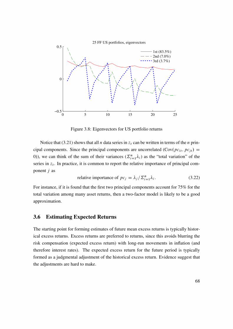
0 5 10 15 20 25−0.5
0
0.525 FF US portfolios, eigenvectors
1st (83.5%)
2nd (7.0%)
3rd (3.7%)
Figure 3.8: Eigenvectors for US portfolio returns
Notice that (3.21) shows that all n data series in zt can be written in terms of the n prin-cipal components. Since the principal components are uncorrelated (Cov.pcit ; pcjt/ D0/), we can think of the sum of their variances (˙n
iD1�i ) as the “total variation” of theseries in zt . In practice, it is common to report the relative importance of principal com-ponent j as
relative importance of pcj D �j=˙niD1�i : (3.22)
For instance, if it is found that the first two principal components account for 75% for thetotal variation among many asset returns, then a two-factor model is likely to be a goodapproximation.
3.6 Estimating Expected Returns
The starting point for forming estimates of future mean excess returns is typically histor-ical excess returns. Excess returns are preferred to returns, since this avoids blurring therisk compensation (expected excess return) with long-run movements in inflation (andtherefore interest rates). The expected excess return for the future period is typicallyformed as a judgmental adjustment of the historical excess return. Evidence suggest thatthe adjustments are hard to make.
68

It is typically hard to predict movements (around the mean) of asset returns, but a fewvariables seem to have some predictive power, for instance, the slope of the yield curve,the earnings/price yield, and the book value–market value ratio. Still, the predictive poweris typically low.
Makridakis, Wheelwright, and Hyndman (1998) 10.1 show that there is little evidencethat the average stock analyst beats (on average) the market (a passive index portfolio).In fact, less than half of the analysts beat the market. However, there are analysts whichseem to outperform the market for some time, but the autocorrelation in over-performanceis weak. The evidence from mutual funds is similar. For them it is typically also foundthat their portfolio weights do not anticipate price movements.
It should be remembered that many analysts also are sales persons: either of a stock(for instance, since the bank is underwriting an offering) or of trading services. It couldwell be that their objective function is quite different from minimizing the squared forecasterrors—or whatever we typically use in order to evaluate their performance. (The numberof litigations in the US after the technology boom/bust should serve as a strong reminderof this.)
3.7 Estimation on Subsamples
To capture time-variation in the regression coefficients, it is fairly common to run theregression
yt D x0tb C "t (3.23)
on a longer and longer data set (“recursive estimation”). In the standard recursive es-timation, the first estimation is done on the sample t D 1; 2; : : : ; � ; while the secondestimation is done on t D 1; 2; : : : ; �; � C 1; and so forth until we use the entire samplet D 1 : : : ; T . In the “backwards recursive estimate” we instead keep the end-point fixedand use more and more of old data. That is, the first sample could be T � �; : : : ; T ; thesecond T � � � 1; : : : ; T ; and so forth.
Alterntively, a moving data window (“rolling samples”) could be used. In this case,the first sample is t D 1; 2; : : : ; � ; but the second is on t D 2; : : : ; �; � C 1, that is, bydropping one observation at the start when the sample is extended at the end. See Figure
3.9 for an illustration.An alternative is to apply an exponentially weighted moving average (EMA) esti-
69
mator, which uses all data points since the beginning of the sample—but where recentobservations carry larger weights. The weight for data in period t is �T�t where T is thelatest observation and 0 < � < 1, where a smaller value of � means that old data carrieslow weights. In practice, this means that we define
Qxt D xt�T�t and Qyt D yt�T�t (3.24)
and then estimateQyt D Qx0tb C "t : (3.25)
Notice that also the constant (in xt ) should be scaled in the same way. (Clearly, thismethod is strongly related to the GLS approach used when residuals are heteroskedastic.Also, the idea of down weighting old data is commonly used to estimate time-varyingvolatility of returns as in the RISK metrics method.)
Estimation on subsamples is not only a way of getting a more recent/modern estimate,but also a way to gauge the historical range and volatility in the betas—which may beimportant for putting some discipline on judgemental forecasts.
See Figures 3.9–3.10 for an illustration.
3.8 Robust Estimation�
3.8.1 Robust Means, Variances and Correlations
Outliers and other extreme observations can have very decisive influence on the estimatesof the key statistics needed for financial analysis, including mean returns, variances, co-variances and also regression coefficients.
The perhaps best way to solve these problems is to carefully analyse the data—andthen decide which data points to exclude. Alternatively, robust estimators can be appliedinstead of the traditional ones.
To estimate the mean, the sample average can be replaced by the median or a trimmed
mean (where the x% lowest and highest observations are excluded).Similarly, to estimate the variance, the sample standard deviation can be replaced by
the interquartile range (the difference between the 75th and the 25th percentiles), dividedby 1:35
StdRobust D Œquantile.0:75/ � quantile.0:25/�=1:35; (3.26)
70
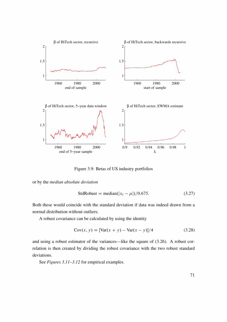
1960 1980 2000
1
1.5
2
β of HiTech sector, recursive
end of sample
1960 1980 2000
1
1.5
2
β of HiTech sector, backwards recursive
start of sample
1960 1980 2000
1
1.5
2
β of HiTech sector, 5−year data window
end of 5−year sample
0.9 0.92 0.94 0.96 0.98 1
1
1.5
2
β of HiTech sector, EWMA estimate
λ
Figure 3.9: Betas of US industry portfolios
or by the median absolute deviation
StdRobust D median.jxt � �j/=0:675: (3.27)
Both these would coincide with the standard deviation if data was indeed drawn from anormal distribution without outliers.
A robust covariance can be calculated by using the identity
Cov.x; y/ D ŒVar.x C y/ � Var.x � y/�=4 (3.28)
and using a robust estimator of the variances—like the square of (3.26). A robust cor-relation is then created by dividing the robust covariance with the two robust standarddeviations.
See Figures 3.11–3.12 for empirical examples.
71

1
NoDur Durbl Manuf Enrgy HiTec Telcm Shops Hlth Utils Other
Month
ly r
eturn
s, %
Distribution of betas estimated on moving 5−year data windows
Monthly data 1947:1−2009:12
Figure 3.10: Distribution of betas of US industry portfolios (estimated on 5-year datawindows)
3.8.2 Robust Regression Coefficients
Reference: Amemiya (1985) 4.6The least absolute deviations (LAD) estimator miminizes the sum of absolute residu-
als (rather than the squared residuals)
OLAD D arg min
b
TXtD1
ˇyt � x0tb
ˇ(3.29)
This estimator involve non-linearities, but a simple iteration works nicely. It is typicallyless sensitive to outliers. (There are also other ways to estimate robust regression coeffi-cients.) This is illustrated in Figure 3.13.
See Figure 3.14 for an empirical example.If we assume that the median of the true residual, ut , is zero, then we (typically) have
pT . OLAD�ˇ0/!d N
�0; f .0/�2˙�1xx =4
�, where ˙xx D plim
XT
tD1xtx0t=T; (3.30)
72

A B C D E F G H I J
0.06
0.07
0.08
0.09
0.1
0.11m
ean e
xce
ss r
eturn
US industry portfolios, ERe
Monthly data 1947:1−2009:12
mean
median
Figure 3.11: Mean excess returns of US industry portfolios
where f .0/ is the value of the pdf of the residual at zero. Unless we know this densityfunction (or else we would probably have used MLE instead of LAD), we need to estimateit—for instance with a kernel density method.
Example 3.7 (N.0; �2/) When ut � N.0; �2), then f .0/ D 1=p2��2, so the covari-
ance matrix in (3.30) becomes ��2˙�1xx =2. This is �=2 times larger than when using
LS.
Remark 3.8 (Algorithm for LAD) The LAD estimator can be written
OLAD D arg min
ˇ
TXtD1
wt Out.b/2, wt D 1= j Out.b/j ; with Out.b/ D yt � x0t Ob
so it is a weighted least squares where both yt and xt are multiplied by 1= j Out.b/j. It can
be shown that iterating on LS with the weights given by 1= j Out.b/j, where the residuals
are from the previous iteration, converges very quickly to the LAD estimator.
Some alternatives to LAD: least median squares (LMS), and least trimmed squares
73

A B C D E F G H I J
0.12
0.14
0.16
0.18
0.2st
d
US industry portfolios, Std
Monthly data 1947:1−2009:12
std
iqr/1.35
Figure 3.12: Volatility of US industry portfolios
(LTS) estimators which solve
OLMS D arg min
ˇ
�median
� Ou2t �� , with Out D yt � x0t Ob (3.31)
OLTS D arg min
ˇ
hXiD1
Ou2i , Ou21 � Ou22 � ::: and h � T: (3.32)
Note that the LTS estimator in (3.32) minimizes the sum of the h smallest squared resid-uals.
Bibliography
Amemiya, T., 1985, Advanced econometrics, Harvard University Press, Cambridge, Mas-sachusetts.
Elton, E. J., M. J. Gruber, S. J. Brown, and W. N. Goetzmann, 2010, Modern portfolio
theory and investment analysis, John Wiley and Sons, 8th edn.
Greene, W. H., 2003, Econometric analysis, Prentice-Hall, Upper Saddle River, NewJersey, 5th edn.
74

−3 −2 −1 0 1 2 3−2
−1.5
−1
−0.5
0
0.5
1
1.5
2
OLS vs LAD of y = 0.75*x + u
x
y
y: −1.125 −0.750 1.750 1.125
x: −1.500 −1.000 1.000 1.500
Data
OLS (0.25 0.90)
LAD (0.00 0.75)
Figure 3.13: Data and regression line from OLS and LAD
Makridakis, S., S. C. Wheelwright, and R. J. Hyndman, 1998, Forecasting: methods and
applications, Wiley, New York, 3rd edn.
75
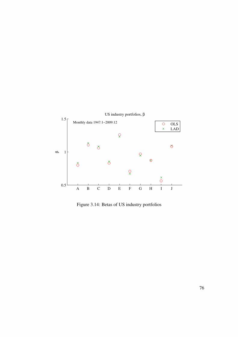
A B C D E F G H I J0.5
1
1.5
β
US industry portfolios, β
Monthly data 1947:1−2009:12
OLS
LAD
Figure 3.14: Betas of US industry portfolios
76
.D..3
4 Testing CAPM and Multifactor Models
Reference: Elton, Gruber, Brown, and Goetzmann (2010) 15More advanced material is denoted by a star (�). It is not required reading.
4.1 Market Model
The basic implication of CAPM is that the expected excess return of an asset (�ei ) islinearly related to the expected excess return on the market portfolio (�em) according to
�ei D ˇi�em, where ˇi D Cov .Ri ; Rm/Var .Rm/
: (4.1)
Let Reit D Rit � Rf t be the excess return on asset i in excess over the riskfree asset,and let Remt be the excess return on the market portfolio. CAPM with a riskfree returnsays that ˛i D 0 in
Reit D ˛i C biRemt C "it , where E "it D 0 and Cov.Remt ; "it/ D 0: (4.2)
The two last conditions are automatically imposed by LS. Take expectations to get
E�Reit� D ˛i C bi E
�Remt
�: (4.3)
Notice that the LS estimate of bi is the sample analogue to ˇi in (4.1). It is then clear thatCAPM implies that ˛i D 0, which is also what empirical tests of CAPM focus on.
This test of CAPM can be given two interpretations. If we assume that Rmt is thecorrect benchmark (the tangency portfolio for which (4.1) is true by definition), then itis a test of whether asset Rit is correctly priced. This is typically the perspective inperformance analysis of mutual funds. Alternatively, if we assume that Rit is correctlypriced, then it is a test of the mean-variance efficiency of Rmt . This is the perspective ofCAPM tests.
The t-test of the null hypothesis that ˛i D 0 uses the fact that, under fairly mild
77
conditions, the t-statistic has an asymptotically normal distribution, that is
O iStd. O i/
d! N.0; 1/ under H0 W ˛i D 0: (4.4)
Note that this is the distribution under the null hypothesis that the true value of the inter-cept is zero, that is, that CAPM is correct (in this respect, at least).
The test assets are typically portfolios of firms with similar characteristics, for in-stance, small size or having their main operations in the retail industry. There are twomain reasons for testing the model on such portfolios: individual stocks are extremelyvolatile and firms can change substantially over time (so the beta changes). Moreover,it is of interest to see how the deviations from CAPM are related to firm characteristics(size, industry, etc), since that can possibly suggest how the model needs to be changed.
The results from such tests vary with the test assets used. For US portfolios, CAPMseems to work reasonably well for some types of portfolios (for instance, portfolios basedon firm size or industry), but much worse for other types of portfolios (for instance, port-folios based on firm dividend yield or book value/market value ratio). Figure 4.1 showssome results for US industry portfolios.
4.1.1 Interpretation of the CAPM Test
Instead of a t-test, we can use the equivalent chi-square test
O 2iVar. O i/
d! �21 under H0: ˛i D 0: (4.5)
Tables (A.2)–(A.1) list critical values for t- and chi-square testsIt is quite straightforward to use the properties of minimum-variance frontiers (see
Gibbons, Ross, and Shanken (1989), and also MacKinlay (1995)) to show that the teststatistic in (4.5) can be written
O 2iVar. O i/
D .SRc/2 � .SRm/2
Œ1C .SRm/2�=T; (4.6)
where SRm is the Sharpe ratio of the market portfolio (as before) and SRc is the Sharperatio of the tangency portfolio when investment in both the market return and asset i ispossible. (Recall that the tangency portfolio is the portfolio with the highest possibleSharpe ratio.) If the market portfolio has the same (squared) Sharpe ratio as the tangency
78

0 0.5 1 1.50
5
10
15US industry portfolios, 1970:1−2010:9
β
Mea
n e
xce
ss r
eturn
A
BC
D
EFGH
I J
0 5 10 150
5
10
15US industry portfolios, 1970:1−2010:9
Predicted mean excess return (with α=0)
Mea
n e
xce
ss r
eturn
A
BC
D
EFGH
I J
Excess market return: 5.2%
all A (NoDur)B (Durbl)C (Manuf)D (Enrgy)E (HiTec)F (Telcm)G (Shops)H (Hlth )I (Utils)J (Other)
alpha NaN 3.53
−0.95 0.78 4.14
−1.67 1.53 1.20 1.99 2.68
−0.46
pval 0.08 0.01 0.64 0.44 0.07 0.38 0.39 0.44 0.27 0.15 0.69
StdErr NaN 8.90 13.38 6.37 14.65 12.18 11.39 9.88 11.71 11.80 7.21
CAPM
Factor: US market
α and StdErr are in annualized %
Figure 4.1: CAPM regressions on US industry indices
portfolio of the mean-variance frontier of Rit and Rmt (so the market portfolio is mean-variance efficient also when we take Rit into account) then the test statistic, O 2i =Var. O i/,is zero—and CAPM is not rejected.
Proof. (�Proof of (4.6)) From the CAPM regression (4.2) we have
Cov
"Reit
Remt
#D"ˇ2i �
2m C Var."it/ ˇi�
2m
ˇi�2m �2m
#, and
"�ei
�em
#D"˛i C ˇi�em
�em
#:
Suppose we use this information to construct a mean-variance frontier for both Rit andRmt , and we find the tangency portfolio, with excess return Rect . It is straightforward toshow that the square of the Sharpe ratio of the tangency portfolio is �e0˙�1�e, where�e is the vector of expected excess returns and ˙ is the covariance matrix. By using thecovariance matrix and mean vector above, we get that the squared Sharpe ratio for the
79
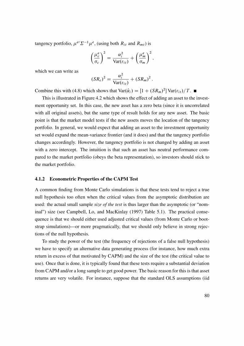
tangency portfolio, �e0˙�1�e, (using both Rit and Rmt ) is��ec�c
�2D ˛2i
Var."it/C��em�m
�2;
which we can write as
.SRc/2 D ˛2i
Var."it/C .SRm/2 :
Combine this with (4.8) which shows that Var. O i/ D Œ1C .SRm/2�Var."it/=T .This is illustrated in Figure 4.2 which shows the effect of adding an asset to the invest-
ment opportunity set. In this case, the new asset has a zero beta (since it is uncorrelatedwith all original assets), but the same type of result holds for any new asset. The basicpoint is that the market model tests if the new assets moves the location of the tangencyportfolio. In general, we would expect that adding an asset to the investment opportunityset would expand the mean-variance frontier (and it does) and that the tangency portfoliochanges accordingly. However, the tangency portfolio is not changed by adding an assetwith a zero intercept. The intuition is that such an asset has neutral performance com-pared to the market portfolio (obeys the beta representation), so investors should stick tothe market portfolio.
4.1.2 Econometric Properties of the CAPM Test
A common finding from Monte Carlo simulations is that these tests tend to reject a truenull hypothesis too often when the critical values from the asymptotic distribution areused: the actual small sample size of the test is thus larger than the asymptotic (or “nom-inal”) size (see Campbell, Lo, and MacKinlay (1997) Table 5.1). The practical conse-quence is that we should either used adjusted critical values (from Monte Carlo or boot-strap simulations)—or more pragmatically, that we should only believe in strong rejec-tions of the null hypothesis.
To study the power of the test (the frequency of rejections of a false null hypothesis)we have to specify an alternative data generating process (for instance, how much extrareturn in excess of that motivated by CAPM) and the size of the test (the critical value touse). Once that is done, it is typically found that these tests require a substantial deviationfrom CAPM and/or a long sample to get good power. The basic reason for this is that assetreturns are very volatile. For instance, suppose that the standard OLS assumptions (iid
80

0 0.05 0.1 0.150
0.05
0.1
MV frontiers before and after (α=0)
Std
Mea
n
Solid curves: 2 assets,
Dashed curves: 3 assets
0 0.05 0.1 0.150
0.05
0.1
MV frontiers before and after (α=0.05)
Std
Mea
n
0 0.05 0.1 0.150
0.05
0.1
MV frontiers before and after (α=−0.04)
Std
Mea
n
The new asset has the abnormal return α
compared to the market (of 2 assets)
Means 0.0800 0.0500 α + β(ERm
−Rf)
Cov matrix
0.0256 0.0000 0.0000 0.0000 0.0144 0.0000 0.0000 0.0000 0.0144
Tang portf
N = 2 0.47 0.53
NaN
α=0
0.47 0.53 0.00
α=0.05
0.31 0.34 0.34
α=−0.04
0.82 0.91
−0.73
Figure 4.2: Effect on MV frontier of adding assets
residuals that are independent of the market return) are correct. Then, it is straightforwardto show that the variance of Jensen’s alpha is
Var. O i/ D"1C .�em/
2
Var�Rem
�#Var."it/=T (4.7)
D Œ1C .SRm/2�Var."it/=T; (4.8)
where SRm is the Sharpe ratio of the market portfolio. We see that the uncertainty aboutthe alpha is high when the residual is volatile and when the sample is short, but also whenthe Sharpe ratio of the market is high. Note that a large market Sharpe ratio means thatthe market asks for a high compensation for taking on risk. A bit uncertainty about howrisky asset i is then translates in a large uncertainty about what the risk-adjusted returnshould be.
81

Example 4.1 Suppose we have monthly data with bi D 0:2% (that is, 0:2%�12 D 2:4%per year), Std ."it/ D 3% (that is, 3%�p12 � 10% per year) and a market Sharpe ratio
of 0:15 (that is, 0:15 � p12 � 0:5 per year). (This corresponds well to US CAPM
regressions for industry portfolios.) A significance level of 10% requires a t-statistic (4.4)
of at least 1.65, so0:2p
1C 0:1523=pT � 1:65 or T � 626:
We need a sample of at least 626 months (52 years)! With a sample of only 26 years (312
months), the alpha needs to be almost 0.3% per month (3.6% per year) or the standard
deviation of the residual just 2% (7% per year). Notice that cumulating a 0.3% return
over 25 years means almost 2.5 times the initial value.
Proof. (�Proof of (4.8)) Consider the regression equation yt D x0tb C "t . With iiderrors that are independent of all regressors (also across observations), the LS estimator,ObLs, is asymptotically distributed as
pT . ObLs � b/ d! N.0; �2˙�1xx /, where �2 D Var."t/ and ˙xx D plim˙T
tD1xtx0t=T:
When the regressors are just a constant (equal to one) and one variable regressor, ft , soxt D Œ1; ft �0, then we have
˙xx D EPT
tD1xtx0t=T D E
1
T
PTtD1
"1 ft
ft f 2t
#D"
1 EftEft Ef 2t
#, so
�2˙�1xx D�2
Ef 2t � .Eft/2"
Ef 2t �Eft�Eft 1
#D �2
Var.ft/
"Var.ft/C .Eft/2 �Eft
�Eft 1
#:
(In the last line we use Var.ft/ D Ef 2t � .Eft/2:)
4.1.3 Several Assets
In most cases there are several (n) test assets, and we actually want to test if all the ˛i (fori D 1; 2; :::; n) are zero. Ideally we then want to take into account the correlation of thedifferent alphas.
While it is straightforward to construct such a test, it is also a bit messy. As a quickway out, the following will work fairly well. First, test each asset individually. Second,form a few different portfolios of the test assets (equally weighted, value weighted) and
82
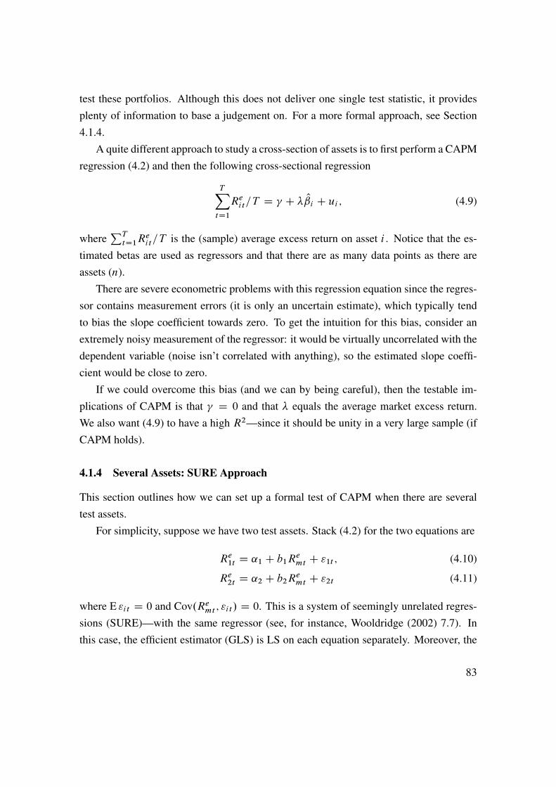
test these portfolios. Although this does not deliver one single test statistic, it providesplenty of information to base a judgement on. For a more formal approach, see Section4.1.4.
A quite different approach to study a cross-section of assets is to first perform a CAPMregression (4.2) and then the following cross-sectional regression
TXtD1
Reit=T D C � Oi C ui ; (4.9)
wherePT
tD1Reit=T is the (sample) average excess return on asset i . Notice that the es-
timated betas are used as regressors and that there are as many data points as there areassets (n).
There are severe econometric problems with this regression equation since the regres-sor contains measurement errors (it is only an uncertain estimate), which typically tendto bias the slope coefficient towards zero. To get the intuition for this bias, consider anextremely noisy measurement of the regressor: it would be virtually uncorrelated with thedependent variable (noise isn’t correlated with anything), so the estimated slope coeffi-cient would be close to zero.
If we could overcome this bias (and we can by being careful), then the testable im-plications of CAPM is that D 0 and that � equals the average market excess return.We also want (4.9) to have a high R2—since it should be unity in a very large sample (ifCAPM holds).
4.1.4 Several Assets: SURE Approach
This section outlines how we can set up a formal test of CAPM when there are severaltest assets.
For simplicity, suppose we have two test assets. Stack (4.2) for the two equations are
Re1t D ˛1 C b1Remt C "1t ; (4.10)
Re2t D ˛2 C b2Remt C "2t (4.11)
where E "it D 0 and Cov.Remt ; "it/ D 0. This is a system of seemingly unrelated regres-sions (SURE)—with the same regressor (see, for instance, Wooldridge (2002) 7.7). Inthis case, the efficient estimator (GLS) is LS on each equation separately. Moreover, the
83

covariance matrix of the coefficients is particularly simple.To see what the covariances of the coefficients are, write the regression equation for
asset 1 (4.10) on a traditional form
Re1t D x0tˇ1 C "1t , where xt D"1
Remt
#; ˇ1 D
"˛1
b1
#; (4.12)
and similarly for the second asset (and any further assets).Define
Oxx D
XT
tD1xtx0t=T , and O�ij D
XT
tD1O"it O"jt=T; (4.13)
where O"it is the fitted residual of asset i . The key result is then that the (estimated)asymptotic covariance matrix of the vectors Oi and Oj (for assets i and j ) is
Cov. Oi ; Oj / D O�ij O �1xx =T: (4.14)
(In many text books, this is written O�ij .X 0X/�1.)The null hypothesis in our two-asset case is
H0 W ˛1 D 0 and ˛2 D 0: (4.15)
In a large sample, the estimator is normally distributed (this follows from the fact thatthe LS estimator is a form of sample average, so we can apply a central limit theorem).Therefore, under the null hypothesis we have the following result. From (4.8) we knowthat the upper left element of ˙�1xx =T equals Œ1C .SRm/2�=T . Then"
O1O2
#� N
"0
0
#;
"�11 �12
�12 �22
#Œ1C .SRm/2�=T
!(asymptotically). (4.16)
In practice we use the sample moments for the covariance matrix. Notice that the zeromeans in (4.16) come from the null hypothesis: the distribution is (as usual) constructedby pretending that the null hypothesis is true. In practice we use the sample moments forthe covariance matrix. Notice that the zero means in (4.16) come from the null hypothesis:the distribution is (as usual) constructed by pretending that the null hypothesis is true.
We can now construct a chi-square test by using the following fact.
Remark 4.2 If the n � 1 vector y � N.0;˝/, then y 0˝�1y � �2n.
84

To apply this, form the test static
T
"O1O2
#0Œ1C .SRm/2��1
"�11 �12
�12 �22
#�1 " O1O2
#� �22: (4.17)
This can also be transformed into an F test, which might have better small sample prop-erties.
4.1.5 Representative Results of the CAPM Test
One of the more interesting studies is Fama and French (1993) (see also Fama and French(1996)). They construct 25 stock portfolios according to two characteristics of the firm:the size (by market capitalization) and the book-value-to-market-value ratio (BE/ME). InJune each year, they sort the stocks according to size and BE/ME. They then form a 5� 5matrix of portfolios, where portfolio ij belongs to the i th size quintile and the j th BE/MEquintile. Tables 4.1–4.2 summarize some basic properties of these portfolios.
Book value/Market value1 2 3 4 5
Size 1 5.3 10.7 11.6 13.3 16.22 4.6 8.5 10.9 10.7 12.03 5.0 8.6 8.9 10.4 12.44 6.3 6.7 8.5 9.6 10.15 5.1 6.6 6.8 6.5 8.3
Table 4.1: Mean excess returns (annualised %), US data 1957:1–2010:9. Size 1: smallest20% of the stocks, Size 5: largest 20% of the stocks. B/M 1: the 20% of the stocks withthe smallest ratio of book to market value (growth stocks). B/M 5: the 20% of the stockswith the highest ratio of book to market value (value stocks).
They run a traditional CAPM regression on each of the 25 portfolios (monthly data1963–1991)—and then study if the expected excess returns are related to the betas as theyshould according to CAPM (recall that CAPM implies EReit D ˇi� where � is the riskpremium (excess return) on the market portfolio).
However, it is found that there is almost no relation between EReit and ˇi (there isa cloud in the ˇi � EReit space, see Cochrane (2001) 20.2, Figure 20.9). This is dueto the combination of two features of the data. First, within a BE/ME quintile, there is
85

Book value/Market value1 2 3 4 5
Size 1 1.4 1.2 1.1 1.0 1.02 1.4 1.2 1.1 1.0 1.23 1.4 1.1 1.0 1.0 1.14 1.3 1.1 1.0 1.0 1.15 1.1 1.0 1.0 0.9 0.9
Table 4.2: Beta against the market portfolio, US data 1957:1–2010:9. Size 1: smallest20% of the stocks, Size 5: largest 20% of the stocks. B/M 1: the 20% of the stocks withthe smallest ratio of book to market value (growth stocks). B/M 5: the 20% of the stockswith the highest ratio of book to market value (value stocks).
−20 −10 0 10 200
0.05
0.1Histogram of small growth stocks
mean, std: 0.44 8.44
Monthly excess return, %
−20 −10 0 10 200
0.05
0.1Histogram of large value stocks
mean, std: 0.69 5.00
Monthly excess return, %
Monthly data on two U.S. indices, 1957:1−2010:9
Sample size: 645
Figure 4.3: Comparison of small growth stock and large value stocks
a positive relation (across size quantiles) between EReit and ˇi—as predicted by CAPM(see Cochrane (2001) 20.2, Figure 20.10). Second, within a size quintile there is a negativerelation (across BE/ME quantiles) between EReit and ˇi—in stark contrast to CAPM (seeCochrane (2001) 20.2, Figure 20.11).
Figure 4.1 shows some results for US industry portfolios and Figures 4.4–4.6 for USsize/book-to-market portfolios.
86

4 6 8 10 12 14 16 18
4
6
8
10
12
14
16
18
Predicted mean excess return (CAPM), %
Mea
n e
xce
ss r
eturn
, %
US data 1957:1−2010:9
25 FF portfolios (B/M and size)
p−value for test of model: 0.00
Figure 4.4: CAPM, FF portfolios
4.1.6 Representative Results on Mutual Fund Performance
Mutual fund evaluations (estimated ˛i ) typically find (i) on average neutral performance(or less: trading costs&fees); (ii) large funds might be worse; (iii) perhaps better perfor-mance on less liquid (less efficient?) markets; and (iv) there is very little persistence inperformance: ˛i for one sample does not predict ˛i for subsequent samples (except forbad funds).
4.2 Several Factors
In multifactor models, (4.2) is still valid—provided we reinterpret bi and Remt as vectors,so biRemt stands for bioReot C bipRept C :::
Reit D ˛ C bioReot C bipRept C :::C "it : (4.18)
87
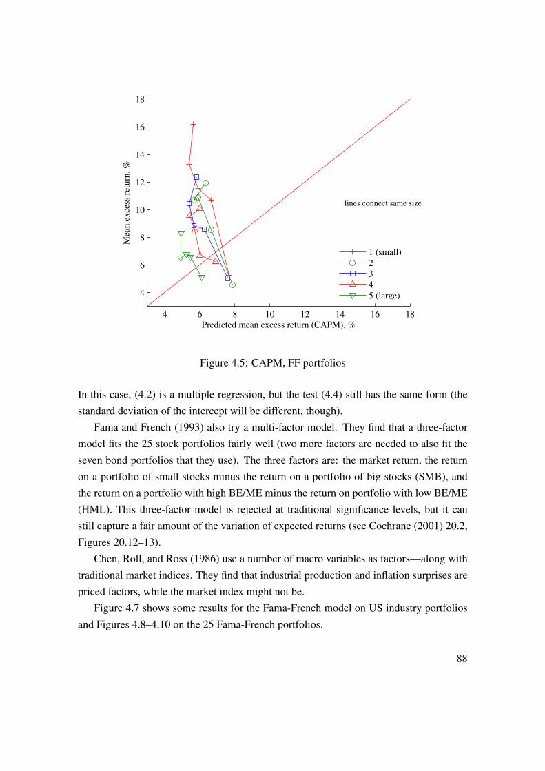
4 6 8 10 12 14 16 18
4
6
8
10
12
14
16
18
Predicted mean excess return (CAPM), %
Mea
n e
xce
ss r
eturn
, %
lines connect same size
1 (small)
2
3
4
5 (large)
Figure 4.5: CAPM, FF portfolios
In this case, (4.2) is a multiple regression, but the test (4.4) still has the same form (thestandard deviation of the intercept will be different, though).
Fama and French (1993) also try a multi-factor model. They find that a three-factormodel fits the 25 stock portfolios fairly well (two more factors are needed to also fit theseven bond portfolios that they use). The three factors are: the market return, the returnon a portfolio of small stocks minus the return on a portfolio of big stocks (SMB), andthe return on a portfolio with high BE/ME minus the return on portfolio with low BE/ME(HML). This three-factor model is rejected at traditional significance levels, but it canstill capture a fair amount of the variation of expected returns (see Cochrane (2001) 20.2,Figures 20.12–13).
Chen, Roll, and Ross (1986) use a number of macro variables as factors—along withtraditional market indices. They find that industrial production and inflation surprises arepriced factors, while the market index might not be.
Figure 4.7 shows some results for the Fama-French model on US industry portfoliosand Figures 4.8–4.10 on the 25 Fama-French portfolios.
88
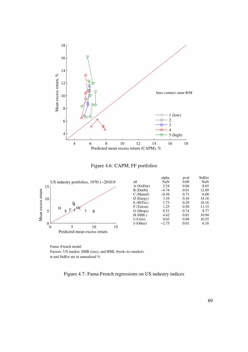
4 6 8 10 12 14 16 18
4
6
8
10
12
14
16
18
Predicted mean excess return (CAPM), %
Mea
n e
xce
ss r
eturn
, %
lines connect same B/M
1 (low)
2
3
4
5 (high)
Figure 4.6: CAPM, FF portfolios
0 5 10 150
5
10
15US industry portfolios, 1970:1−2010:9
Predicted mean excess return
Mea
n e
xce
ss r
eturn
A
BC
D
E FGH
I J
all A (NoDur)B (Durbl)C (Manuf)D (Enrgy)E (HiTec)F (Telcm)G (Shops)H (Hlth )I (Utils)J (Other)
alpha NaN 2.54
−4.74 −0.36 3.16 1.73 1.25 0.51 4.42 0.03
−2.75
pval 0.00 0.06 0.01 0.71 0.16 0.29 0.50 0.74 0.01 0.98 0.01
StdErr NaN 8.65 12.09 6.08 14.16 10.16 11.15 9.77 10.94 10.55 6.18
Fama−French model
Factors: US market, SMB (size), and HML (book−to−market)
α and StdErr are in annualized %
Figure 4.7: Fama-French regressions on US industry indices
89
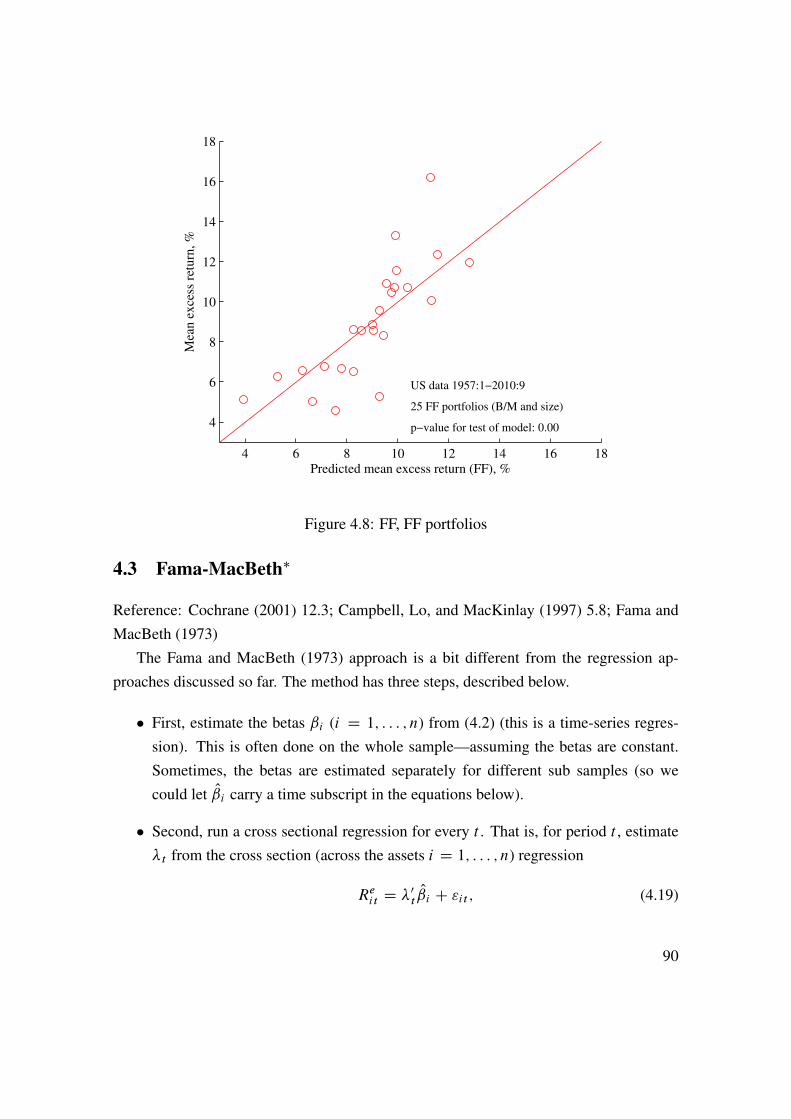
4 6 8 10 12 14 16 18
4
6
8
10
12
14
16
18
Predicted mean excess return (FF), %
Mea
n e
xce
ss r
eturn
, %
US data 1957:1−2010:9
25 FF portfolios (B/M and size)
p−value for test of model: 0.00
Figure 4.8: FF, FF portfolios
4.3 Fama-MacBeth�
Reference: Cochrane (2001) 12.3; Campbell, Lo, and MacKinlay (1997) 5.8; Fama andMacBeth (1973)
The Fama and MacBeth (1973) approach is a bit different from the regression ap-proaches discussed so far. The method has three steps, described below.
� First, estimate the betas ˇi (i D 1; : : : ; n) from (4.2) (this is a time-series regres-sion). This is often done on the whole sample—assuming the betas are constant.Sometimes, the betas are estimated separately for different sub samples (so wecould let Oi carry a time subscript in the equations below).
� Second, run a cross sectional regression for every t . That is, for period t , estimate�t from the cross section (across the assets i D 1; : : : ; n) regression
Reit D �0t Oi C "it ; (4.19)
90

4 6 8 10 12 14 16 18
4
6
8
10
12
14
16
18
Predicted mean excess return (FF), %
Mea
n e
xce
ss r
eturn
, %
lines connect same size
1 (small)
2
3
4
5 (large)
Figure 4.9: FF, FF portfolios
where Oi are the regressors. (Note the difference to the traditional cross-sectionalapproach discussed in (4.9), where the second stage regression regressed EReit onOi , while the Fama-French approach runs one regression for every time period.)
� Third, estimate the time averages
O"i D 1
T
TXtD1
O"it for i D 1; : : : ; n, (for every asset) (4.20)
O� D 1
T
TXtD1
O�t : (4.21)
The second step, using Oi as regressors, creates an errors-in-variables problem sinceOi are estimated, that is, measured with an error. The effect of this is typically to bias the
estimator of �t towards zero (and any intercept, or mean of the residual, is biased upward).One way to minimize this problem, used by Fama and MacBeth (1973), is to let the assetsbe portfolios of assets, for which we can expect some of the individual noise in the first-
91

4 6 8 10 12 14 16 18
4
6
8
10
12
14
16
18
Predicted mean excess return (FF), %
Mea
n e
xce
ss r
eturn
, %
lines connect same B/M
1 (low)
2
3
4
5 (high)
Figure 4.10: FF, FF portfolios
step regressions to average out—and thereby make the measurement error in Oi smaller.If CAPM is true, then the return of an asset is a linear function of the market return and anerror which should be uncorrelated with the errors of other assets—otherwise some factoris missing. If the portfolio consists of 20 assets with equal error variance in a CAPMregression, then we should expect the portfolio to have an error variance which is 1/20thas large.
We clearly want portfolios which have different betas, or else the second step regres-sion (4.19) does not work. Fama and MacBeth (1973) choose to construct portfoliosaccording to some initial estimate of asset specific betas. Another way to deal with theerrors-in-variables problem is to adjust the tests.
We can test the model by studying if "i D 0 (recall from (4.20) that "i is the timeaverage of the residual for asset i , "it ), by forming a t-test O"i=Std.O"i/. Fama and MacBeth(1973) suggest that the standard deviation should be found by studying the time-variationin O"it . In particular, they suggest that the variance of O"it (not O"i ) can be estimated by the
92

(average) squared variation around its mean
Var.O"it/ D 1
T
TXtD1
.O"it � O"i/2 : (4.22)
Since O"i is the sample average of O"it , the variance of the former is the variance of the latterdivided by T (the sample size)—provided O"it is iid. That is,
Var.O"i/ D 1
TVar.O"it/ D 1
T 2
TXtD1
.O"it � O"i/2 : (4.23)
A similar argument leads to the variance of O�
Var. O�/ D 1
T 2
TXtD1
. O�t � O�/2: (4.24)
Fama and MacBeth (1973) found, among other things, that the squared beta is notsignificant in the second step regression, nor is a measure of non-systematic risk.
A Statistical Tables
n Critical values10% 5% 1%
10 1.81 2.23 3.1720 1.72 2.09 2.8530 1.70 2.04 2.7540 1.68 2.02 2.7050 1.68 2.01 2.6860 1.67 2.00 2.6670 1.67 1.99 2.6580 1.66 1.99 2.6490 1.66 1.99 2.63100 1.66 1.98 2.63Normal 1.64 1.96 2.58
Table A.1: Critical values (two-sided test) of t distribution (different degrees of freedom)and normal distribution.
93

n Critical values10% 5% 1%
1 2.71 3.84 6.632 4.61 5.99 9.213 6.25 7.81 11.344 7.78 9.49 13.285 9.24 11.07 15.096 10.64 12.59 16.817 12.02 14.07 18.488 13.36 15.51 20.099 14.68 16.92 21.6710 15.99 18.31 23.21
Table A.2: Critical values of chisquare distribution (different degrees of freedom, n).
Bibliography
Campbell, J. Y., A. W. Lo, and A. C. MacKinlay, 1997, The econometrics of financial
markets, Princeton University Press, Princeton, New Jersey.
Chen, N.-F., R. Roll, and S. A. Ross, 1986, “Economic forces and the stock market,”Journal of Business, 59, 383–403.
Cochrane, J. H., 2001, Asset pricing, Princeton University Press, Princeton, New Jersey.
Elton, E. J., M. J. Gruber, S. J. Brown, and W. N. Goetzmann, 2010, Modern portfolio
theory and investment analysis, John Wiley and Sons, 8th edn.
Fama, E., and J. MacBeth, 1973, “Risk, return, and equilibrium: empirical tests,” Journal
of Political Economy, 71, 607–636.
Fama, E. F., and K. R. French, 1993, “Common risk factors in the returns on stocks andbonds,” Journal of Financial Economics, 33, 3–56.
Fama, E. F., and K. R. French, 1996, “Multifactor explanations of asset pricing anoma-lies,” Journal of Finance, 51, 55–84.
Gibbons, M., S. Ross, and J. Shanken, 1989, “A test of the efficiency of a given portfolio,”Econometrica, 57, 1121–1152.
94

MacKinlay, C., 1995, “Multifactor models do not explain deviations from the CAPM,”Journal of Financial Economics, 38, 3–28.
Wooldridge, J. M., 2002, Econometric analysis of cross section and panel data, MITPress.
95
5 Time Series Analysis
Reference: Newbold (1995) 17 or Pindyck and Rubinfeld (1998) 13.5, 16.1–2, and 17.2More advanced material is denoted by a star (�). It is not required reading.
5.1 Descriptive Statistics
The sth autocovariance of yt is estimated by
bCov .yt ; yt�s/ DPT
tD1 .yt � Ny/ .yt�s � Ny/ =T , where Ny DPTtD1yt=T: (5.1)
The conventions in time series analysis are that we use the same estimated (using all data)mean in both places and that we divide by T .
The sth autocorrelation is estimated as
O�s DbCov
�yt ; yt�p
�cStd .yt/
2: (5.2)
Compared with a traditional estimate of a correlation we here impose that the standarddeviation of yt and yt�p are the same (which typically does not make much of a differ-ence).
The sampling properties of O�s are complicated, but there are several useful large sam-ple results for Gaussian processes (these results typically carry over to processes whichare similar to the Gaussian—a homoskedastic process with finite 6th moment is typicallyenough, see Priestley (1981) 5.3 or Brockwell and Davis (1991) 7.2-7.3). When the trueautocorrelations are all zero (not �0, of course), then for any i and j different from zero
pT
"O�iO�j
#!d N
"0
0
#;
"1 0
0 1
#!: (5.3)
This result can be used to construct tests for both single autocorrelations (t-test or �2 test)and several autocorrelations at once (�2 test). In particular,
pT O�s d! N.0; 1/; (5.4)
96

sopT O�s can be used as a t-stat.
Example 5.1 (t-test) We want to test the hypothesis that �1 D 0. Since the N.0; 1/ dis-
tribution has 5% of the probability mass below -1.65 and another 5% above 1.65, we
can reject the null hypothesis at the 10% level ifpT j O�1j > 1:65. With T D 100, we
therefore need j O�1j > 1:65=p100 D 0:165 for rejection, and with T D 1000 we need
j O�1j > 1:65=p1000 � 0:052.
The Box-Pierce test follows directly from the result in (5.3), since it shows thatpT O�i
andpT O�j are iid N(0,1) variables. Therefore, the sum of the square of them is distributed
as a �2 variable. The test statistics typically used is
QL D TLXsD1
O�2s !d �2L: (5.5)
Example 5.2 (Box-Pierce) Let O�1 D 0:165, and T D 100, so Q1 D 100 � 0:1652 D2:72. The 10% critical value of the �21 distribution is 2.71, so the null hypothesis of no
autocorrelation is rejected.
The choice of lag order in (5.5), L, should be guided by theoretical considerations, butit may also be wise to try different values. There is clearly a trade off: too few lags maymiss a significant high-order autocorrelation, but too many lags can destroy the power ofthe test (as the test statistics is not affected much by increasing L, but the critical valuesincrease).
The pth partial autocorrelation is discussed in Section 5.3.6.
5.2 White Noise
The white noise process is the basic building block used in most other time series models.It is characterized by a zero mean, a constant variance, and no autocorrelation
E "t D 0Var ."t/ D �2, and
Cov ."t�s; "t/ D 0 if s ¤ 0. (5.6)
97
If, in addition, "t is normally distributed, then it is said to be Gaussian white noise. Thisprocess can clearly not be forecasted.
To construct a variable that has a non-zero mean, we can form
yt D �C "t ; (5.7)
where � is a constant. This process is most easily estimated by estimating the samplemean and variance in the usual way (as in (5.1) with p D 0).
5.3 Autoregression (AR)
5.3.1 AR(1)
In this section we study the first-order autoregressive process, AR(1), in some detail inorder to understand the basic concepts of autoregressive processes. The process is as-sumed to have a zero mean (or is demeaned, that an original variable minus its mean, forinstance yt D xt � Nxt )—but it is straightforward to put in any mean or trend.
An AR(1) isyt D ayt�1 C "t ; with Var."t/ D �2; (5.8)
where "t is the white noise process in (5.6) which is uncorrelated with yt�1. If �1 < a <1, then the effect of a shock eventually dies out: yt is stationary.
The AR(1) model can be estimated with OLS (since "t and yt�1 are uncorrelated) andthe usual tools for testing significance of coefficients and estimating the variance of theresidual all apply.
The basic properties of an AR(1) process are (provided jaj < 1)
Var .yt/ D �2=.1 � a2/ (5.9)
Corr .yt ; yt�s/ D as; (5.10)
so the variance and autocorrelation are increasing in a (assuming a > 0).See Figure 5.1 for an illustration.
Remark 5.3 (Autocorrelation and autoregression). Notice that the OLS estimate of a in
(5.8) is essentially the same as the sample autocorrelation coefficient in (5.2). This follows
from the fact that the slope coefficient is bCov .yt ; yt�1/ =cVar.yt�1/. The denominator
98

0 2 4 6 8 10−1
−0.5
0
0.5
1
Autocorrelations
Periods
AR(1), 0.85
MA(1), 0.85
0 2 4 6 8 10−1
−0.5
0
0.5
1
Partial autocorrelations
Periods
AR(1), 0.85
MA(1), 0.85
0 2 4 6 8 10−1
−0.5
0
0.5
1
Autocorrelations
Periods
AR(1), −0.85
MA(1), −0.85
0 2 4 6 8 10−1
−0.5
0
0.5
1
Partial autocorrelations
Periods
AR(1), −0.85
MA(1), −0.85
Figure 5.1: Autocorrelations and partial autocorrelations
can be a bit different since a few data points are left out in the OLS estimation, but the
difference is likely to be small.
Example 5.4 With a D 0:85 and �2 D 0:52, we have Var .yt/ D 0:25=.1�0:852/ � 0:9,
which is much larger than the variance of the residual. (Why?)
If a D 1 in (5.8), then we get a random walk. It is clear from the previous analysisthat a random walk is non-stationary—that is, the effect of a shock never dies out. Thisimplies that the variance is infinite and that the standard tools for testing coefficients etc.are invalid. The solution is to study changes in y instead: yt �yt�1. In general, processeswith the property that the effect of a shock never dies out are called non-stationary or unitroot or integrated processes. Try to avoid them.
See Figure 5.2 for an example.
99

0 20 40 60
−0.5
0
0.5
Return = a + b*lagged Return, slope
Return horizon (months)
Slope with 90% conf band
US stock returns 1926:1−2010:4
0 20 40 600
0.05
0.1
Return = a + b*lagged Return, R2
Return horizon (months)
Figure 5.2: Predicting US stock returns (various investment horizons) with lagged returns.
5.3.2 More on the Properties of an AR(1) Process�
Solve (5.8) backwards by repeated substitution
yt D a.ayt�2 C "t�1/„ ƒ‚ …yt�1
C "t (5.11)
D a2yt�2 C a"t�1 C "t (5.12)::: (5.13)
D aKC1yt�K�1 CKXsD0
as"t�s: (5.14)
The factor aKC1yt�K�1 declines monotonically to zero if 0 < a < 1 as K increases, anddeclines in an oscillating fashion if �1 < a < 0. In either case, the AR(1) process iscovariance stationary and we can then take the limit as K !1 to get
yt D "t C a"t�1 C a2"t�2 C :::
D1XsD0
as"t�s: (5.15)
Since "t is uncorrelated over time, yt�1 and "t are uncorrelated. We can thereforecalculate the variance of yt in (5.8) as the sum of the variances of the two components on
100

the right hand side
Var .yt/ D Var .ayt�1/C Var ."t/
D a2 Var .yt�1/C Var ."t/
D Var ."t/ =.1 � a2/; since Var .yt�1/ D Var .yt/ . (5.16)
In this calculation, we use the fact that Var .yt�1/ and Var .yt/ are equal. Formally, thisfollows from that they are both linear functions of current and past "s terms (see (5.15)),which have the same variance over time ("t is assumed to be white noise).
Note from (5.16) that the variance of yt is increasing in the absolute value of a, whichis illustrated in Figure 5.3. The intuition is that a large jaj implies that a shock have effectover many time periods and thereby create movements (volatility) in y.
Similarly, the covariance of yt and yt�1 is
Cov .yt ; yt�1/ D Cov .ayt�1 C "t ; yt�1/D aCov .yt�1; yt�1/
D aVar .yt/ : (5.17)
We can then calculate the first-order autocorrelation as
Corr .yt ; yt�1/ D Cov .yt ; yt�1/Std.yt/Std.yt�1/
D a: (5.18)
It is straightforward to show that
Corr .yt ; yt�s/ D Corr .ytCs; yt/ D as: (5.19)
5.3.3 Forecasting with an AR(1)
Suppose we have estimated an AR(1). To simplify the exposition, we assume that weactually know a and Var."t/, which might be a reasonable approximation if they wereestimated on long sample.
We want to forecast ytC1 using information available in t . From (5.8) we get
ytC1 D ayt C "tC1: (5.20)
101

0 2 4 6 8 10−5
0
5Forecast with 90% conf band
Forecasting horizon
Intial value: 3
0 2 4 6 8 10−5
0
5Forecast with 90% conf band
Forecasting horizon
Intial value: 0
AR(1) model: yt+1
= 0.85yt + ε
t+1, σ = 0.5
Figure 5.3: Properties of AR(1) process
Since the best guess of "tC1 is that it is zero, the best forecast and the associated forecasterror are
Et ytC1 D ayt , and (5.21)
ytC1 � Et ytC1 D "tC1 with variance �2. (5.22)
We may also want to forecast ytC2 using the information in t . To do that note that(5.8) gives
ytC2 D aytC1 C "tC2D a.ayt C "tC1/„ ƒ‚ …
ytC1
C "tC2
D a2yt C a"tC1 C "tC2: (5.23)
Since the Et "tC1 and Et "tC2 are both zero, we get that
Et ytC2 D a2yt ; and (5.24)
ytC2 � Et ytC2 D a"tC1 C "tC2 with variance a2�2 C �2: (5.25)
102

More generally, we have
Et ytCs D asyt , (5.26)
Var .ytCs � Et ytCs/ D�1C a2 C a4 C :::C a2.s�1/
��2 (5.27)
D a2s � 1a2 � 1 �
2: (5.28)
Example 5.5 If yt D 3; a D 0:85 and � D 0:5, then the forecasts and the forecast error
variances become
Horizon s Et ytCs Var .ytCs � Et ytCs/1 0:85 � 3 D 2:55 0:25
2 0:852 � 3 D 2:17 �0:852 C 1� � 0:52 D 0:43
25 0:8525 � 3 D 0:05 0:8550�10:852�1
� 0:52 D 0:90
Notice that the point forecast converge towards zero and the variance of the forecast error
variance to the unconditional variance (see Example 5.4).
If the shocks "t , are normally distributed, then we can calculate 90% confidence in-tervals around the point forecasts in (5.21) and (5.24) as
90% confidence band of Et ytC1 W ayt ˙ 1:65 � � (5.29)
90% confidence band of Et ytC2 W a2yt ˙ 1:65 �pa2�2 C �2: (5.30)
(Recall that 90% of the probability mass is within the interval �1:65 to 1:65 in the N(0,1)distribution). To get 95% confidence bands, replace 1.65 by 1.96. Figure 5.3 gives anexample.
Example 5.6 Continuing Example 5.5, we get the following 90% confidence bands
Horizon s
1 2:55˙ 1:65 �p0:25 � Œ1:7; 3:4�2 2:17˙ 1:65 �p0:43 � Œ1:1; 3:2�25 0:05˙ 1:65 �p0:90 � Œ�1:5; 1:6�
:
Remark 5.7 (White noise as special case of AR(1).) When a D 0 in (5.8), then the
AR(1) collapses to a white noise process. The forecast is then a constant (zero) for all
103

forecasting horizons, see (5.26), and the forecast error variance is also the same for all
horizons, see (5.28).
5.3.4 Adding a Constant to the AR(1)
The discussion of the AR(1) worked with a zero mean variable, but that was just forconvenience (to make the equations shorter). One way to work with a variable xt witha non-zero mean, is to first estimate its sample mean Nxt and then let the yt in the AR(1)model (5.8) be a demeaned variable yt D xt � Nxt .
To include a constant � in the theoretical expressions, we just need to substitute xt��for yt everywhere. For instance, in (5.8) we would get
xt � � D a .xt�1 � �/C "t or
xt D .1 � a/�C axt�1 C "t : (5.31)
Estimation by LS will therefore give an intercept that equals .1 � a/� and a slope coef-ficient that equals a.
5.3.5 AR(p)
The pth-order autoregressive process, AR(p), is a straightforward extension of the AR(1)
yt D a1yt�1 C a2yt�2 C :::apyt�p C "t : (5.32)
All the previous calculations can be made on this process as well—it is just a bit messier.This process can also be estimated with OLS since "t is uncorrelated with lags of yt .Adding a constant is straightforward by substituting xt � � for yt everywhere
5.3.6 Partial Autocorrelations
The pth partial autocorrelation tries to measure the direct relation between yt and yt�p,where the indirect effects of yt�1; :::; yt�pC1 are eliminated. For instance, if yt is gen-erated by an AR(1) model, then the 2nd autocorrelation is a2, whereas the 2nd partialautocorrelation is zero. The partial autocorrelation is therefore a way to gauge how manylags that are needed in an AR(p) model.
104
In practice, the first partial autocorrelation is estimated by a in an AR(1)
yt D ayt�1 C "t : (5.33)
The second partial autocorrelation is estimated by the second slope coefficient (a2) in anAR(2)
yt D a1yt�1 C a2yt�2 C "t ; (5.34)
and so forth. The general pattern is that the pth partial autocorrelation is estimated by theslope coefficient of the pth lag in an AR(p), where we let p go from 1,2,3...
See Figure 5.1 for an illustration.
5.3.7 Forecasting with an AR(2)�
As an example, consider making a forecast of ytC1 based on the information in t by usingan AR(2)
ytC1 D a1yt C a2yt�1 C "tC1: (5.35)
This immediately gives the one-period point forecast
Et ytC1 D a1yt C a2yt�1: (5.36)
We can use (5.35) to write ytC2 as
ytC2 D a1ytC1 C a2yt C "tC2D a1.a1yt C a2yt�1 C "tC1/„ ƒ‚ …
ytC1
C a2yt C "tC2
D .a21 C a2/yt C a1a2yt�1 C a1"tC1 C "tC2: (5.37)
Figure 5.4 gives an empirical example.The expressions for the forecasts and forecast error variances quickly get somewhat
messy—and even more so with an AR of higher order than two. There is a simple, andapproximately correct, shortcut that can be taken. Note that both the one-period and two-period forecasts are linear functions of yt and yt�1. We could therefore estimate the
105
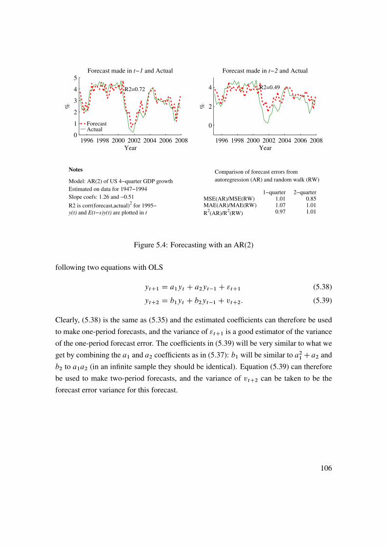
1996 1998 2000 2002 2004 2006 20080
1
2
3
4
5Forecast made in t−1 and Actual
ForecastActual
Year
%
R2=0.72
1996 1998 2000 2002 2004 2006 2008
0
2
4
Forecast made in t−2 and Actual
Year
%
R2=0.49
Notes
Model: AR(2) of US 4−quarter GDP growth
Estimated on data for 1947−1994
Slope coefs: 1.26 and −0.51
R2 is corr(forecast,actual)2 for 1995−
y(t) and E(t−s)y(t) are plotted in t
Comparison of forecast errors from
autoregression (AR) and random walk (RW)
MSE(AR)/MSE(RW)MAE(AR)/MAE(RW)
R2(AR)/R
2(RW)
1−quarter 1.01 1.07 0.97
2−quarter 0.85 1.01 1.01
Figure 5.4: Forecasting with an AR(2)
following two equations with OLS
ytC1 D a1yt C a2yt�1 C "tC1 (5.38)
ytC2 D b1yt C b2yt�1 C vtC2: (5.39)
Clearly, (5.38) is the same as (5.35) and the estimated coefficients can therefore be usedto make one-period forecasts, and the variance of "tC1 is a good estimator of the varianceof the one-period forecast error. The coefficients in (5.39) will be very similar to what weget by combining the a1 and a2 coefficients as in (5.37): b1 will be similar to a21Ca2 andb2 to a1a2 (in an infinite sample they should be identical). Equation (5.39) can thereforebe used to make two-period forecasts, and the variance of vtC2 can be taken to be theforecast error variance for this forecast.
106
5.4 Moving Average (MA)
A qth-order moving average process is
yt D "t C �1"t�1 C :::C �q"t�q; (5.40)
where the innovation "t is white noise (usually Gaussian). It is straightforward to add aconstant to capture a non-zero mean.
Estimation of MA processes is typically done by setting up the likelihood functionand then using some numerical method to maximize it; LS does not work at all since theright hand side variables are unobservable. This is one reason why MA models play alimited role in applied work. Moreover, most MA models can be well approximated byan AR model of low order.
The autocorrelations and partial autocorrelations (for different lags) can help us gaugeif the time series looks more like an AR or an MA. In an AR(p) model, the autocorrela-tions decay to zero for long lags, while the pC1 partial autocorrelation (and beyond) goesabruptly to zero. The reverse is true for an MA model. See Figure 5.1 for an illustration.
5.5 ARMA(p,q)
Autoregressive-moving average models add a moving average structure to an AR model.For instance, an ARMA(2,1) could be
yt D a1yt�1 C a2yt�2 C "t C �1"t�1; (5.41)
where "t is white noise. This type of model is much harder to estimate than the autoregres-sive model (LS cannot be used). The appropriate specification of the model (number oflags of yt and "t ) is often unknown. The Box-Jenkins methodology is a set of guidelinesfor arriving at the correct specification by starting with some model, study the autocorre-lation structure of the fitted residuals and then changing the model.
It is straightforward to add a constant to capture a non-zero mean.Most ARMA models can be well approximated by an AR model—provided we add
some extra lags. Since AR models are so simple to estimate, this approximation approachis often used.
107

Remark 5.8 In an ARMA model, both the autocorrelations and partial autocorrelations
decay to zero for long lags.
5.6 VAR(p)
The vector autoregression is a multivariate version of an AR(1) process: we can think ofyt and "t in (5.32) as vectors and the ai as matrices.
For instance the VAR(1) of two variables (xt and zt ) is (in matrix form)"xtC1
ztC1
#D"a11 a12
a21 a22
#"xt
zt
#C""xtC1
"ztC1
#; (5.42)
or equivalently
xtC1 D a11xt C a12zt C "xtC1; and (5.43)
ztC1 D a21xt C a22zt C "ztC1: (5.44)
Both (5.43) and (5.44) are regression equations, which can be estimated with OLS(since "xtC1 and "ztC1 are uncorrelated with xt and zt ).
With the information available in t , that is, information about xt and zt , (5.43) and(5.44) can be used to forecast one step ahead as
Et xtC1 D a11xt C a12zt (5.45)
Et ztC1 D a21xt C a22zt : (5.46)
We also want to make a forecast of xtC2 based on the information in t . Clearly, itmust be the case that
Et xtC2 D a11 Et xtC1 C a12 Et ztC1 (5.47)
Et ztC2 D a21 Et xtC1 C a22 Et ztC1: (5.48)
We already have values for Et xtC1 and Et ztC1 from (5.45) and (5.46) which we can use.
108

For instance, for Et xtC2 we get
Et xtC2 D a11.a11xt C a12zt/„ ƒ‚ …Et xtC1
C a12.a21xt C a22zt/„ ƒ‚ …Et ztC1
D �a211 C a12a21� xt C .a12a22 C a11a12/ zt : (5.49)
This has the same form as the one-period forecast in (5.45), but with other coefficients.Note that all we need to make the forecasts (for both t C 1 and t C 2) are the values inperiod t (xt and zt ). This follows from that (5.42) is a first-order system where the valuesof xt and zt summarize all relevant information about the future that is available in t .
The forecast uncertainty about the one-period forecast is simple: the forecast errorxtC1 � Et xtC1 D "xtC1. The two-period forecast error, xtC2 � Et xtC2, is a linearcombination of "xtC1, "ztC1, and "xtC2. The calculations of the forecasting error variance(as well as for the forecasts themselves) quickly get messy. This is even more true whenthe VAR system is of a higher order.
As for the AR(p) model, a practical way to get around the problem with messy calcu-lations is to estimate a separate model for each forecasting horizon. In a large sample, thedifference between the two ways is trivial. For instance, suppose the correct model is theVAR(1) in (5.42) and that we want to forecast x one and two periods ahead. From (5.45)and (5.49) we see that the regression equations should be of the form
xtC1 D ı1xt C ı2zt C utC1, and (5.50)
xtC2 D 1xt C 2zt C wtCs: (5.51)
With estimated coefficients (OLS can be used), it is straightforward to calculate forecastsand forecast error variances.
In a more general VAR(p) model we need to include p lags of both x and z in theregression equations (p D 1 in (5.50) and (5.51)).
5.6.1 Granger Causality
If zt can help predict future x, over and above what lags of x itself can, then z is said toGranger Cause x. This is a statistical notion of causality, and may not necessarily havemuch to do with economic causality (Christmas cards may Granger cause Christmas).In (5.50) z does Granger cause x if ı2 ¤ 0, which can be tested with an F-test. More
109
generally, there may be more lags of both x and z in the equation, so we need to test if allcoefficients on different lags of z are zero.
5.7 Non-stationary Processes
5.7.1 Introduction
A trend-stationary process can be made stationary by subtracting a linear trend. Thesimplest example is
yt D �C ˇt C "t (5.52)
where "t is white noise.A unit root process can be made stationary only by taking a difference. The simplest
example is the random walk with drift
yt D �C yt�1 C "t ; (5.53)
where "t is white noise. The name “unit root process” comes from the fact that the largesteigenvalues of the canonical form (the VAR(1) form of the AR(p)) is one. Such a processis said to be integrated of order one (often denoted I(1)) and can be made stationary bytaking first differences.
Example 5.9 (Non-stationary AR(2).) The process yt D 1:5yt�1 � 0:5yt�2 C "t can be
written "yt
yt�1
#D"1:5 �0:51 0
#"yt�1
yt�2
#C""t
0
#;
where the matrix has the eigenvalues 1 and 0.5 and is therefore non-stationary. Note that
subtracting yt�1 from both sides gives yt�yt�1 D 0:5 .yt�1 � yt�2/C"t , so the variable
xt D yt � yt�1 is stationary.
The distinguishing feature of unit root processes is that the effect of a shock never
vanishes. This is most easily seen for the random walk. Substitute repeatedly in (5.53) to
110

get
yt D �C .�C yt�2 C "t�1/C "t:::
D t�C y0 CtXsD1
"s: (5.54)
The effect of "t never dies out: a non-zero value of "t gives a permanent shift of the levelof yt . This process is clearly non-stationary. A consequence of the permanent effect ofa shock is that the variance of the conditional distribution grows without bound as theforecasting horizon is extended. For instance, for the random walk with drift, (5.54), thedistribution conditional on the information in t D 0 is N
�y0 C t�; s�2
�if the innova-
tions are Gaussian. This means that the expected change is t� and that the conditionalvariance grows linearly with the forecasting horizon. The unconditional variance is there-fore infinite and the standard results on inference are not applicable.
In contrast, the conditional distribution from the trend stationary model, (5.52), isN�st; �2
�.
A process could have two unit roots (integrated of order 2: I(2)). In this case, we needto difference twice to make it stationary. Alternatively, a process can also be explosive,that is, have eigenvalues outside the unit circle. In this case, the impulse response functiondiverges.
Example 5.10 (Two unit roots.) Suppose yt in Example (5.9) is actually the first differ-
ence of some other series, yt D zt � zt�1. We then have
zt � zt�1 D 1:5 .zt�1 � zt�2/ � 0:5 .zt�2 � zt�3/C "tzt D 2:5zt�1 � 2zt�2 C 0:5zt�3 C "t ;
which is an AR(3) with the following canonical form264 zt
zt�1
zt�2
375 D264 2:5 �2 0:5
1 0 0
0 1 0
375264 zt�1
zt�2
zt�3
375C264 "t
0
0
375 :The eigenvalues are 1, 1, and 0.5, so zt has two unit roots (integrated of order 2: I(2) and
111
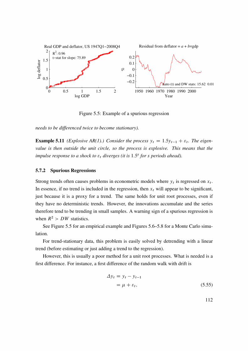
0 0.5 1 1.5 20
0.5
1
1.5
2Real GDP and deflator, US 1947Q1−2008Q4
log GDP
log d
efla
tor
R2: 0.96
t−stat for slope: 75.89
1950 1960 1970 1980 1990 2000
−0.2
−0.1
0
0.1
0.2
Residual from deflator = a + b×gdp
Year
%
Auto (t) and DW stats: 15.62 0.01
Figure 5.5: Example of a spurious regression
needs to be differenced twice to become stationary).
Example 5.11 (Explosive AR(1).) Consider the process yt D 1:5yt�1 C "t . The eigen-
value is then outside the unit circle, so the process is explosive. This means that the
impulse response to a shock to "t diverges (it is 1:5s for s periods ahead).
5.7.2 Spurious Regressions
Strong trends often causes problems in econometric models where yt is regressed on xt .In essence, if no trend is included in the regression, then xt will appear to be significant,just because it is a proxy for a trend. The same holds for unit root processes, even ifthey have no deterministic trends. However, the innovations accumulate and the seriestherefore tend to be trending in small samples. A warning sign of a spurious regression iswhen R2 > DW statistics.
See Figure 5.5 for an empirical example and Figures 5.6–5.8 for a Monte Carlo simu-lation.
For trend-stationary data, this problem is easily solved by detrending with a lineartrend (before estimating or just adding a trend to the regression).
However, this is usually a poor method for a unit root processes. What is needed is afirst difference. For instance, a first difference of the random walk with drift is
�yt D yt � yt�1D �C "t ; (5.55)
112

−0.5 0 0.50
2
4
6
Distribution of bLS
, ρ=0.2
b
−0.5 0 0.50
2
4
6
Distribution of bLS
, ρ=1
b
Illustration of spurious regressions
y and x are uncorrelated AR(1) processes:
Model: yt = ρy
t−1 + ε
t and x
t = ρx
t−1 + η
t
where εt and η
t are uncorrelated
bLS
is the LS estimate of b in
yt = a + bx
t + u
t, T=200
Figure 5.6: Distribution of LS estimator when yt and xt are independent AR(1) processes
which is white noise (any finite difference, like yt � yt�s, will give a stationary series),so we could proceed by applying standard econometric tools to �yt .
One may then be tempted to try first-differencing all non-stationary series, since itmay be hard to tell if they are unit root process or just trend-stationary. For instance, afirst difference of the trend stationary process, (5.52), gives
yt � yt�1 D ˇ C "t � "t�1: (5.56)
Its unclear if this is an improvement: the trend is gone, but the errors are now of MA(1)type (in fact, non-invertible, and therefore tricky, in particular for estimation).
5.7.3 Testing for a Unit Root�
Suppose we run an OLS regression of
yt D ayt�1 C "t ; (5.57)
113

0 0.2 0.4 0.6 0.8 10
10
20
30
40
50
Distribution of R2, ρ=0.2
R2
0 0.2 0.4 0.6 0.8 10
5
10
15
Distribution of R2, ρ=1
R2
−0.2 0 0.2 0.4 0.6 0.80
5
10
15
Distribution of autocorr, ρ=0.2
Autocorrelations of residuals
−0.2 0 0.2 0.4 0.6 0.80
5
10
15
Distribution of autocorr, ρ=1
Autocorrelation of residuals
Figure 5.7: Distribution of R2 and autorrelation of residuals. See Figure 5.6
−5 0 50
0.1
0.2
0.3
0.4
Distribution of t−stat, ρ=0.2
t−stat
−10 0 10 200
0.05
0.1
Distribution of t−stat, ρ=1
t−stat
Figure 5.8: Distribution of t-statistics. See Figure 5.6
where the true value of jaj < 1. The asymptotic distribution of the LS estimator is
pT . Oa � a/ � N �
0; 1 � a2� : (5.58)
114
(The variance follows from the standard OLS formula where the variance of the estimatoris �2 .X 0X=T /�1. Here plimX 0X=T DVar.yt/ which we know is �2=
�1 � a2�).
It is well known (but not easy to show) that when a D 1, then Oa is biased towardszero in small samples. In addition, the asymptotic distribution is no longer (5.58). Infact, there is a discontinuity in the limiting distribution as we move from a stationary toa non-stationary variable. This, together with the small sample bias means that we haveto use simulated critical values for testing the null hypothesis of a D 1 based on the OLSestimate from (5.57).
In practice, the approach is to run the regression (5.57) with a constant (and perhapseven a time trend), calculate the test statistic
DF D Oa � 1Std. Oa/; (5.59)
and reject the null of non-stationarity if DF is less than the critical values published byDickey and Fuller (�2:86 at the 5% level if the regression has a constant, and �3:41 ifthe regression includes a trend).
With more dynamics (to capture any serial correlation in "t in (5.57)), do an aug-
mented DickeyFuller test (ADF)
yt D ı C �1yt�1 C �2yt�2 C "2t , or
�yt D ı C .�1 C �2 � 1/ yt�1 � �2�yt�1 C "2t ; (5.60)
and test if �1C �2 � 1 D 0 (against the alternative, < 0) The critical values are as for theDF test. If "2t is autocorrelated, then add further lags.
In principle, distinguishing between a stationary and a non-stationary series is verydifficult (and impossible unless we restrict the class of processes, for instance, to anAR(2)), since any sample of a non-stationary process can be arbitrary well approximatedby some stationary process et vice versa. The lesson to be learned, from a practical pointof view, is that strong persistence in the data generating process (stationary or not) invali-
dates the usual results on inference. We are usually on safer ground to apply the unit rootresults in this case, even if the process is actually stationary.
115

Bibliography
Brockwell, P. J., and R. A. Davis, 1991, Time series: theory and methods, Springer Verlag,New York, second edn.
Newbold, P., 1995, Statistics for business and economics, Prentice-Hall, 4th edn.
Pindyck, R. S., and D. L. Rubinfeld, 1998, Econometric models and economic forecasts,Irwin McGraw-Hill, Boston, Massachusetts, 4ed edn.
Priestley, M. B., 1981, Spectral analysis and time series, Academic Press.
116

6 Predicting Asset Returns
Reference (medium): Elton, Gruber, Brown, and Goetzmann (2010) 17 (efficient markets)and 26 (earnings estimation)Additional references: Campbell, Lo, and MacKinlay (1997) 2 and 7; Cochrane (2001)20.1
More advanced material is denoted by a star (�). It is not required reading.
6.1 Asset Prices, Random Walks, and the Efficient Market Hypothe-sis
Let Pt be the price of an asset at the end of period t , after any dividend in t has been paid(an ex-dividend price). The gross return (1 C RtC1, like 1.05) of holding an asset withdividends (per current share), DtC1, between t and t C 1 is then defined as
1CRtC1 D PtC1 CDtC1
Pt: (6.1)
The dividend can, of course, be zero in a particular period, so this formulation encom-passes the case of daily stock prices with annual dividend payment.
Remark 6.1 (Conditional expectations) The expected value of the random variable ytC1conditional on the information set in t , Et ytC1 is the best guess of ytC1 using the infor-
mation in t . Example: suppose ytC1 equals xt C "tC1, where xt is known in t , but all we
know about "tC1 in t is that it is a random variable with a zero mean and some (finite)
variance. In this case, the best guess of ytC1 based on what we know in t is equal to xt .
Take expectations of (6.1) based on the information set in t
1C Et RtC1 D Et PtC1 C Et DtC1
Ptor (6.2)
Pt D E tPtC1 C E tDtC1
1C E tRtC1: (6.3)
117
This formulation is only a definition, but it will help us organize the discussion of howasset prices are determined.
This expected return, Et RtC1, is likely to be greater than a riskfree interest rate if theasset has positive systematic (non-diversifiable) risk. For instance, in a CAPM model thiswould manifest itself in a positive “beta.” In an equilibrium setting, we can think of thisas a “required return” needed for investors to hold this asset.
6.1.1 Different Versions of the Efficient Market Hypothesis
The efficient market hypothesis casts a long shadow on every attempt to forecast assetprices. In its simplest form it says that it is not possible to forecast asset prices, but thereare several other forms with different implications. Before attempting to forecast financialmarkets, it is useful to take a look at the logic of the efficient market hypothesis. This willhelp us to organize the effort and to interpret the results.
A modern interpretation of the efficient market hypothesis (EMH) is that the informa-tion set used in forming the market expectations in (6.2) includes all public information.(This is the semi-strong form of the EMH since it says all public information; the strongform says all public and private information; and the weak form says all information inprice and trading volume data.) The implication is that simple stock picking techniquesare not likely to improve the portfolio performance, that is, abnormal returns. Instead,advanced (costly?) techniques are called for in order to gather more detailed informationthan that used in market’s assessment of the asset. Clearly, with a better forecast of thefuture return than that of the market there is plenty of scope for dynamic trading strate-gies. Note that this modern interpretation of the efficient market hypothesis does not ruleout the possibility of forecastable prices or returns. It does rule out that abnormal returnscan be achieved by stock picking techniques which rely on public information.
There are several different traditional interpretations of the EMH. Like the moderninterpretation, they do not rule out the possibility of achieving abnormal returns by usingbetter information than the rest of the market. However, they make stronger assumptionsabout whether prices or returns are forecastable. Typically one of the following is as-sumed to be unforecastable: price changes, returns, or returns in excess of a riskfree rate(interest rate). By unforecastable, it is meant that the best forecast (expected value condi-tional on available information) is a constant. Conversely, if it is found that there is someinformation in t that can predict returns RtC1, then the market cannot price the asset as
118

if Et RtC1 is a constant—at least not if the market forms expectations rationally. We willnow analyze the logic of each of the traditional interpretations.
If price changes are unforecastable, then Et PtC1 � Pt equals a constant. Typically,this constant is taken to be zero so Pt is a martingale. Use Et PtC1 D Pt in (6.2)
Et RtC1 D Et DtC1
Pt: (6.4)
This says that the expected net return on the asset is the expected dividend divided by thecurrent price. This is clearly implausible for daily data since it means that the expectedreturn is zero for all days except those days when the asset pays a dividend (or rather, theday the asset goes ex dividend)—and then there is an enormous expected return for the oneday when the dividend is paid. As a first step, we should probably refine the interpretationof the efficient market hypothesis to include the dividend so that Et.PtC1CDtC1/ D Pt .Using that in (6.2) gives 1 C Et RtC1 D 1, which can only be satisfied if Et RtC1 D 0,which seems very implausible for long investment horizons—although it is probably areasonable approximation for short horizons (a week or less).
If returns are unforecastable, so Et RtC1 D R (a constant), then (6.3) gives
Pt D E tPtC1 C E tDtC1
1CR : (6.5)
The main problem with this interpretation is that it looks at every asset separately andthat outside options are not taken into account. For instance, if the nominal interest ratechanges from 5% to 10%, why should the expected (required) return on a stock be un-changed? In fact, most asset pricing models suggest that the expected return Et RtC1equals the riskfree rate plus compensation for risk.
If excess returns are unforecastable, then the compensation (over the riskfree rate)for risk is constant. The risk compensation is, of course, already reflected in the currentprice Pt , so the issue is then if there is some information in t which is correlated withthe risk compensation in PtC1. Note that such forecastability does not necessarily implyan inefficient market or presence of uninformed traders—it could equally well be due tomovements in risk compensation driven by movements in uncertainty (option prices sug-gest that there are plenty of movements in uncertainty). If so, the forecastability cannot beused to generate abnormal returns (over riskfree rate plus risk compensation). However,it could also be due to exploitable market inefficiencies. Alternatively, you may argue
119

that the market compensates for risk which you happen to be immune to—so you areinterested in the return rather than the risk adjusted return.
This discussion of the traditional efficient market hypothesis suggests that the mostinteresting hypotheses to test are if returns or excess returns are forecastable. In practice,the results for them are fairly similar since the movements in most asset returns are muchgreater than the movements in interest rates.
6.1.2 Martingales and Random Walks�
Further reading: Cuthbertson (1996) 5.3The accumulated wealth in a sequence of fair bets is expected to be unchanged. It is
then said to be a martingale.The time series x is a martingale with respect to an information set˝t if the expected
value of xtCs (s � 1) conditional on the information set ˝t equals xt . (The informationset ˝t is often taken to be just the history of x: xt ; xt�1; :::)
The time series x is a random walk if xtC1 D xt C "tC1, where "t and "tCs areuncorrelated for all s ¤ 0, and E "t D 0. (There are other definitions which require that"t and "tCs have the same distribution.) A random walk is a martingale; the converse isnot necessarily true.
Remark 6.2 (A martingale, but not a random walk). Suppose ytC1 D ytutC1, where utand utCs are uncorrelated for all s ¤ 0, and Et utC1 D 1 . This is a martingale, but not
a random walk.
In any case, the martingale property implies that xtCs D xtC"tCs, where the expectedvalue of "tCs based on ˝t is zero. This is close enough to the random walk to motivatethe random walk idea in most cases.
120
6.2 Autocorrelations
6.2.1 Autocorrelation Coefficients and the Box-Pierce Test
The autocovariances of the yt process can be estimated as
O s D 1
T
TXtD1Cs
.yt � Ny/ .yt�s � Ny/ ; (6.6)
with Ny D 1
T
TXtD1
yt : (6.7)
(We typically divide by T in (6.6) even if we have only T �s full observations to estimate s from.) Autocorrelations are then estimated as
O�s D O s= O 0: (6.8)
The sampling properties of O�s are complicated, but there are several useful large sam-ple results for Gaussian processes (these results typically carry over to processes whichare similar to the Gaussian—a homoskedastic process with finite 6th moment is typicallyenough, see Priestley (1981) 5.3 or Brockwell and Davis (1991) 7.2-7.3). When the trueautocorrelations are all zero (not �0, of course), then for any i and j different from zero
pT
"O�iO�j
#!d N
"0
0
#;
"1 0
0 1
#!: (6.9)
This result can be used to construct tests for both single autocorrelations (t-test or �2 test)and several autocorrelations at once (�2 test).
Example 6.3 (t-test) We want to test the hypothesis that �1 D 0. Since the N.0; 1/ dis-
tribution has 5% of the probability mass below -1.65 and another 5% above 1.65, we
can reject the null hypothesis at the 10% level ifpT j O�1j > 1:65. With T D 100, we
therefore need j O�1j > 1:65=p100 D 0:165 for rejection, and with T D 1000 we need
j O�1j > 1:65=p1000 � 0:052.
The Box-Pierce test follows directly from the result in (6.9), since it shows thatpT O�i
andpT O�j are iid N(0,1) variables. Therefore, the sum of the square of them is distributed
121

as a �2 variable. The test statistics typically used is
QL D TLXsD1
O�2s !d �2L: (6.10)
Example 6.4 (Box-Pierce) Let O�1 D 0:165, and T D 100, so Q1 D 100 � 0:1652 D2:72. The 10% critical value of the �21 distribution is 2.71, so the null hypothesis of no
autocorrelation is rejected.
The choice of lag order in (6.10), L, should be guided by theoretical considerations,but it may also be wise to try different values. There is clearly a trade off: too few lags maymiss a significant high-order autocorrelation, but too many lags can destroy the power ofthe test (as the test statistics is not affected much by increasing L, but the critical valuesincrease).
6.2.2 Autoregressions
An alternative way of testing autocorrelations is to estimate an AR model
yt D c C a1yt�1 C a2yt�2 C :::C apyt�p C "t ; (6.11)
and then test if all slope coefficients (a1; a2; :::; ap) are zero with a �2 or F test. Thisapproach is somewhat less general than the Box-Pierce test, but most stationary timeseries processes can be well approximated by an AR of relatively low order.
See Figure 6.5 for an illustration.The autoregression can also allow for the coefficients to depend on the market situ-
ation. For instance, consider an AR(1), but where the autoregression coefficient may bedifferent depending on the sign of last period’s return
yt D cCaı.yt�1 � 0/yt�1Cbı.yt�1 > 0/yt�1, where ı.q/ D(1 if q is true0 else.
(6.12)
See Figure 6.3 for an illustration.Inference of the slope coefficient in autoregressions on returns for longer data horizons
than the data frequency (for instance, analysis of weekly returns in a data set consistingof daily observations) must be done with care. If only non-overlapping returns are used(use the weekly return for a particular weekday only, say Wednesdays), the standard LS
122
expression for the standard deviation of the autoregressive parameter is likely to be rea-sonable. This is not the case, if overlapping returns (all daily data on weekly returns) areused.
Remark 6.5 (Overlapping returns�) Consider an AR(1) for the two-period return, yt�1Cyt
ytC1 C ytC2 D aC b2 .yt�1 C yt/C "tC2:Two successive observations with non-overlapping returns are then
ytC1 C ytC2 D aC b2 .yt�1 C yt/C "tC2ytC3 C ytC4 D aC b2 .ytC1 C ytC2/C "tC4:
Suppose that yt is not autocorrelated, so the slope coefficient b2 D 0. We can then write
the residuals as
"tC2 D �aC ytC1 C ytC2"tC4 D �aC ytC3 C ytC4;
which are uncorrelated. Compare this to the case where we use overlapping data. Two
successive observations are then
ytC1 C ytC2 D aC b2 .yt�1 C yt/C "tC2ytC2 C ytC3 D aC b2 .yt C ytC1/C "tC3:
As before, b2 D 0 if yt has no autocorrelation, so the residuals become
"tC2 D �aC ytC1 C ytC2"tC3 D �aC ytC2 C ytC3;
which are correlated since ytC2 shows up in both. This demonstrates that overlapping
return data introduces autocorrelation of the residuals—which has to be handled in order
to make correct inference.
123

1990 1995 2000 2005 20100
2
4
6
8SMI
Year
SMI
bill portfolio
1990 1995 2000 2005 2010−10
−5
0
5
10SMI daily excess returns, %
Year
Daily SMI data, 1988:7−2010:9
1st order autocorrelation of returns (daily, weekly, monthly): 0.02 −0.08 0.04
1st order autocorrelation of absolute returns (daily, weekly, monthly): 0.28 0.28 0.17
Figure 6.1: Time series properties of SMI
6.2.3 Autoregressions versus Autocorrelations�
It is straightforward to see the relation between autocorrelations and the AR model whenthe AR model is the true process. This relation is given by the Yule-Walker equations.
For an AR(1), the autoregression coefficient is simply the first autocorrelation coeffi-cient. For an AR(2), yt D a1yt�1 C a2yt�2 C "t , we have264 Cov.yt ; yt/
Cov.yt�1; yt/Cov.yt�2; yt/
375 D264 Cov.yt ; a1yt�1 C a2yt�2 C "t/
Cov.yt�1; a1yt�1 C a2yt�2 C "t/Cov.yt�2; a1yt�1 C a2yt�2 C "t/
375
D
264 a1 Cov.yt ; yt�1/C a2 Cov.yt ; yt�2/C Cov.yt ; "t/a1 Cov.yt�1; yt�1/C a2 Cov.yt�1; yt�2/a1 Cov.yt�2; yt�1/C a2 Cov.yt�2; yt�2/
375 , or
264 0
1
2
375 D264 a1 1 C a2 2 C Var."t/a1 0 C a2 1a1 1 C a2 0
375 : (6.13)
124

1 2 3 4 5−0.1
0
0.1
0.2
0.3Autocorr, daily excess returns
lags (days)
Autocorr with 90% conf band around 0
S&P 500, 1979:1−2010:9
1 2 3 4 5−0.1
0
0.1
0.2
0.3Autocorr, weekly excess returns
lags (weeks)
1 2 3 4 5−0.1
0
0.1
0.2
0.3Autocorr, daily abs(excess returns)
lags (days)
1 2 3 4 5−0.1
0
0.1
0.2
0.3Autocorr, weekly abs(excess returns)
lags (weeks)
Figure 6.2: Predictability of US stock returns
1 2 3 4 5−0.1
−0.05
0
0.05
0.1Autoregression coeff, after negative returns
lags (days)
with 90% conf band around 0
S&P 500 (daily), 1979:1−2010:9
1 2 3 4 5−0.1
−0.05
0
0.05
0.1Autoregression coeff, after positive returns
lags (days)
Figure 6.3: Predictability of US stock returns, results from a regression with interactivedummies
To transform to autocorrelation, divide by 0. The last two equations are then"�1
�2
#D"a1 C a2�1a1�1 C a2
#or
"�1
�2
#D"a1= .1 � a2/a21= .1 � a2/C a2
#: (6.14)
125

1 2 3 4 5−0.1
0
0.1
0.2
0.3
Autocorr, excess returns, smallest decile
lags (days)
1 2 3 4 5−0.1
0
0.1
0.2
0.3
Autocorr, excess returns, 5th decile
lags (days)
1 2 3 4 5−0.1
0
0.1
0.2
0.3
Autocorr, excess returns, largest decile
lags (days)
Autocorr with 90% conf band around 0
US daily data 1979:1−2010:9
Figure 6.4: Predictability of US stock returns, size deciles
If we know the parameters of the AR(2) model (a1, a2, and Var."t/), then we cansolve for the autocorrelations. Alternatively, if we know the autocorrelations, then we cansolve for the autoregression coefficients. This demonstrates that testing if all the autocor-relations are zero is essentially the same as testing if all the autoregressive coefficients arezero. Note, however, that the transformation is non-linear, which may make a differencein small samples.
6.2.4 Variance Ratios
A variance ratio is another way to measure predictability. It is defined as the variance ofa q-period return divided by q times the variance of a 1-period return
VRq DVar
�Pq�1sD0 yt�s
�qVar.yt/
: (6.15)
126
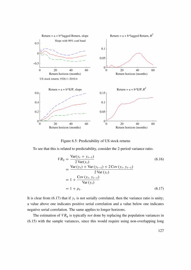
0 20 40 60
−0.5
0
0.5
Return = a + b*lagged Return, slope
Return horizon (months)
Slope with 90% conf band
US stock returns 1926:1−2010:4
0 20 40 600
0.05
0.1
Return = a + b*lagged Return, R2
Return horizon (months)
0 20 40 600
0.2
0.4
0.6Return = a + b*E/P, slope
Return horizon (months)
0 20 40 600
0.05
0.1
0.15Return = a + b*E/P, R
2
Return horizon (months)
Figure 6.5: Predictability of US stock returns
To see that this is related to predictability, consider the 2-period variance ratio.
VR2 D Var.yt C yt�1/2Var.yt/
(6.16)
D Var .yt/C Var .yt�1/C 2Cov .yt ; yt�1/2Var .yt/
D 1C Cov .yt ; yt�1/Var .yt/
D 1C �1: (6.17)
It is clear from (6.17) that if yt is not serially correlated, then the variance ratio is unity;a value above one indicates positive serial correlation and a value below one indicatesnegative serial correlation. The same applies to longer horizons.
The estimation of VRq is typically not done by replacing the population variances in(6.15) with the sample variances, since this would require using non-overlapping long
127

0 20 40 60
0.5
1
1.5
Variance Ratio, 1926−
Return horizon (months)
VR with 90% conf band
0 20 40 60
0.5
1
1.5
Variance Ratio, 1957−
Return horizon (months)
US stock returns 1926:1−2010:4
Confidence bands use asymptotic sampling distribution of VR
Figure 6.6: Variance ratios, US excess stock returns
returns—which wastes a lot of data points. For instance, if we have 24 years of data andwe want to study the variance ratio for the 5-year horizon, then 4 years of data are wasted.Instead, we typically rely on a transformation of (6.15)
VRq DVar
�Pq�1sD0 yt�s
�qVar.yt/
Dq�1X
sD�.q�1/
�1 � jsj
q
��s or
D 1C 2q�1XsD1
�1 � s
q
��s: (6.18)
To estimate VRq, we first estimate the autocorrelation coefficients (using all available datapoints for each estimation) and then calculate (6.18).
Remark 6.6 (�Sampling distribution of bVRq) Under the null hypothesis that there is no
autocorrelation, (6.9) and (6.18) give
pT�bVRq � 1
�!d N
"0;
q�1XsD1
4
�1 � s
q
�2#:
128

Example 6.7 (Sampling distributions of bVR2 and bVR3)pT�bVR2 � 1
�!d N .0; 1/ or bVR2 !d N .1; 1=T /
andpT�bVR3 � 1
�!d N .1; 20=9/ or bVR3 !d N Œ1; .20=9/=T � :
The results in CLM Table 2.5 and 2.6 (weekly CRSP stock index returns, early 1960sto mid 1990s) show variance ratios above one and increasing with the number of lags, q.The results for individual stocks in CLM Table 2.7 show variance ratios close to, or evenbelow, unity. Cochrane Tables 20.5–6 report weak evidence for more mean reversion inmulti-year returns (annual NYSE stock index,1926 to mid 1990s).
See Figure 6.6 for an illustration.
6.3 Other Predictors and Methods
There are many other possible predictors of future stock returns. For instance, both thedividend-price ratio and nominal interest rates have been used to predict long-run returns,and lagged short-run returns on other assets have been used to predict short-run returns.
6.3.1 Lead-Lags
Stock indices have more positive autocorrelation than (most) individual stocks: thereshould therefore be fairly strong cross-autocorrelations across individual stocks. (SeeCampbell, Lo, and MacKinlay (1997) Tables 2.7 and 2.8.) Indeed, this is also what isfound in US data where weekly returns of large size stocks forecast weekly returns ofsmall size stocks.
See Figures 6.7–6.8 for an illustration.
6.3.2 Dividend-Price Ratio as a Predictor
One of the most successful attempts to forecast long-run returns is a regression of futurereturns on the current dividend-price ratio (here in logs)
qXsD1
rtCs D ˛ C ˇq.dt � pt/C "tCq: (6.19)
129
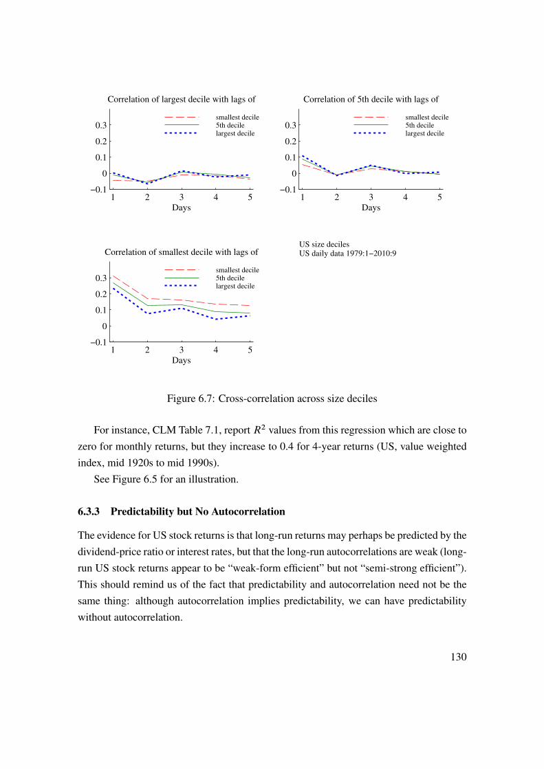
1 2 3 4 5−0.1
0
0.1
0.2
0.3
Correlation of largest decile with lags of
Days
smallest decile5th decile largest decile
1 2 3 4 5−0.1
0
0.1
0.2
0.3
Correlation of 5th decile with lags of
Days
smallest decile5th decile largest decile
1 2 3 4 5−0.1
0
0.1
0.2
0.3
Correlation of smallest decile with lags of
Days
smallest decile5th decile largest decile
US size deciles US daily data 1979:1−2010:9
Figure 6.7: Cross-correlation across size deciles
For instance, CLM Table 7.1, report R2 values from this regression which are close tozero for monthly returns, but they increase to 0.4 for 4-year returns (US, value weightedindex, mid 1920s to mid 1990s).
See Figure 6.5 for an illustration.
6.3.3 Predictability but No Autocorrelation
The evidence for US stock returns is that long-run returns may perhaps be predicted by thedividend-price ratio or interest rates, but that the long-run autocorrelations are weak (long-run US stock returns appear to be “weak-form efficient” but not “semi-strong efficient”).This should remind us of the fact that predictability and autocorrelation need not be thesame thing: although autocorrelation implies predictability, we can have predictabilitywithout autocorrelation.
130
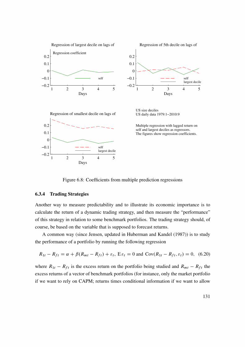
1 2 3 4 5−0.2
−0.1
0
0.1
0.2
Regression of largest decile on lags of
Days
Regression coefficient
self
1 2 3 4 5−0.2
−0.1
0
0.1
0.2
Regression of 5th decile on lags of
Days
self largest decile
1 2 3 4 5−0.2
−0.1
0
0.1
0.2
Regression of smallest decile on lags of
Days
self largest decile
US size deciles US daily data 1979:1−2010:9
Multiple regression with lagged return onself and largest deciles as regressors. The figures show regression coefficients.
Figure 6.8: Coefficients from multiple prediction regressions
6.3.4 Trading Strategies
Another way to measure predictability and to illustrate its economic importance is tocalculate the return of a dynamic trading strategy, and then measure the “performance”of this strategy in relation to some benchmark portfolios. The trading strategy should, ofcourse, be based on the variable that is supposed to forecast returns.
A common way (since Jensen, updated in Huberman and Kandel (1987)) is to studythe performance of a portfolio by running the following regression
R1t �Rf t D ˛ C ˇ.Rmt �Rf t/C "t , E "t D 0 and Cov.R1t �Rf t ; "t/ D 0; (6.20)
where R1t � Rf t is the excess return on the portfolio being studied and Rmt � Rf t theexcess returns of a vector of benchmark portfolios (for instance, only the market portfolioif we want to rely on CAPM; returns times conditional information if we want to allow
131

1 2 3 4 5 6 7 8 9 10 11 12 13 14 15 16 17 18 19 20 21 22 23 24 25
1
2
3
4
5
6
7
8
9
10
11
12
13
14
15
16
17
18
19
20
21
22
23
24
25
0.21
0.22
0.22
0.24
0.27
0.11
0.13
0.11
0.12
0.13
0.06
0.09
0.10
0.10
0.10
0.07
0.10
0.08
0.09
0.08
0.04
0.05
0.04
0.05
0.07
0.21
0.21
0.23
0.24
0.28
0.11
0.13
0.12
0.13
0.13
0.06
0.10
0.11
0.10
0.10
0.06
0.10
0.08
0.09
0.09
0.04
0.05
0.04
0.05
0.07
0.21
0.22
0.23
0.25
0.30
0.11
0.14
0.13
0.14
0.14
0.07
0.11
0.12
0.12
0.12
0.07
0.11
0.10
0.11
0.11
0.06
0.07
0.05
0.06
0.08
0.20
0.22
0.24
0.25
0.30
0.11
0.13
0.12
0.14
0.14
0.07
0.11
0.11
0.11
0.11
0.06
0.10
0.09
0.10
0.11
0.05
0.06
0.04
0.06
0.08
0.19
0.21
0.22
0.24
0.29
0.09
0.12
0.11
0.13
0.14
0.05
0.09
0.10
0.11
0.10
0.05
0.09
0.08
0.09
0.11
0.04
0.05
0.03
0.05
0.07
0.26
0.27
0.27
0.28
0.31
0.17
0.17
0.16
0.16
0.17
0.11
0.14
0.14
0.14
0.13
0.11
0.14
0.12
0.12
0.12
0.09
0.09
0.07
0.08
0.11
0.24
0.26
0.27
0.28
0.32
0.15
0.17
0.16
0.16
0.17
0.11
0.14
0.14
0.15
0.13
0.10
0.14
0.12
0.12
0.13
0.08
0.09
0.07
0.08
0.12
0.24
0.26
0.27
0.29
0.33
0.15
0.17
0.16
0.17
0.17
0.11
0.14
0.15
0.15
0.14
0.09
0.13
0.12
0.12
0.14
0.08
0.09
0.07
0.08
0.11
0.22
0.25
0.26
0.28
0.32
0.14
0.16
0.16
0.17
0.18
0.09
0.14
0.15
0.15
0.13
0.08
0.13
0.12
0.12
0.14
0.07
0.09
0.07
0.08
0.11
0.21
0.24
0.25
0.27
0.32
0.12
0.15
0.15
0.16
0.18
0.09
0.13
0.14
0.15
0.14
0.06
0.12
0.12
0.12
0.14
0.06
0.08
0.06
0.08
0.11
0.27
0.28
0.28
0.30
0.32
0.18
0.19
0.18
0.18
0.18
0.13
0.16
0.16
0.16
0.14
0.13
0.15
0.13
0.13
0.13
0.11
0.10
0.08
0.09
0.12
0.26
0.29
0.29
0.31
0.35
0.19
0.20
0.20
0.20
0.20
0.15
0.18
0.18
0.18
0.17
0.13
0.17
0.16
0.15
0.16
0.11
0.12
0.10
0.11
0.14
0.23
0.26
0.28
0.30
0.33
0.16
0.19
0.19
0.19
0.20
0.12
0.16
0.17
0.17
0.17
0.10
0.15
0.14
0.14
0.16
0.09
0.10
0.09
0.10
0.14
0.24
0.27
0.28
0.30
0.34
0.17
0.19
0.20
0.20
0.21
0.14
0.17
0.17
0.18
0.17
0.11
0.16
0.15
0.15
0.16
0.10
0.11
0.09
0.10
0.13
0.19
0.23
0.24
0.26
0.31
0.12
0.15
0.16
0.17
0.19
0.08
0.13
0.14
0.16
0.15
0.06
0.12
0.12
0.12
0.14
0.04
0.08
0.06
0.08
0.12
0.27
0.28
0.28
0.30
0.32
0.20
0.20
0.19
0.19
0.19
0.15
0.17
0.17
0.17
0.15
0.14
0.16
0.14
0.15
0.14
0.12
0.11
0.09
0.10
0.13
0.24
0.27
0.29
0.30
0.33
0.18
0.21
0.21
0.21
0.21
0.15
0.19
0.18
0.19
0.16
0.12
0.16
0.15
0.15
0.16
0.10
0.11
0.10
0.11
0.13
0.23
0.26
0.28
0.30
0.34
0.17
0.20
0.21
0.21
0.22
0.14
0.18
0.18
0.20
0.17
0.11
0.16
0.16
0.17
0.16
0.10
0.12
0.10
0.13
0.13
0.22
0.25
0.26
0.28
0.32
0.15
0.18
0.19
0.19
0.20
0.12
0.16
0.16
0.17
0.16
0.09
0.14
0.14
0.14
0.15
0.07
0.09
0.07
0.09
0.12
0.21
0.24
0.25
0.26
0.31
0.14
0.16
0.16
0.17
0.19
0.11
0.13
0.14
0.16
0.14
0.08
0.12
0.12
0.12
0.14
0.07
0.08
0.06
0.08
0.10
0.24
0.25
0.26
0.27
0.30
0.18
0.18
0.19
0.18
0.18
0.14
0.17
0.17
0.17
0.15
0.13
0.15
0.14
0.14
0.14
0.11
0.11
0.09
0.11
0.14
0.22
0.24
0.26
0.28
0.31
0.17
0.18
0.20
0.19
0.19
0.14
0.17
0.16
0.17
0.15
0.11
0.15
0.14
0.13
0.14
0.09
0.10
0.08
0.09
0.12
0.23
0.26
0.27
0.28
0.32
0.17
0.19
0.21
0.21
0.21
0.15
0.18
0.18
0.19
0.17
0.11
0.16
0.16
0.15
0.17
0.09
0.11
0.10
0.11
0.13
0.21
0.24
0.27
0.28
0.32
0.16
0.20
0.21
0.22
0.22
0.14
0.18
0.18
0.20
0.17
0.11
0.16
0.16
0.16
0.17
0.09
0.11
0.09
0.11
0.14
0.19
0.22
0.24
0.25
0.29
0.13
0.17
0.18
0.19
0.21
0.11
0.15
0.17
0.18
0.17
0.08
0.13
0.13
0.14
0.16
0.06
0.09
0.07
0.10
0.12
(Auto−)correlation matrix, monthly FF returns
Figure 6.9: Illustration of the cross-autocorrelations, Corr.Rt ; Rt�k/, monthly FF data.Dark colors indicate high correlations, light colors indicate low correlations.
for time-variation in expected benchmark returns). Neutral performance (mean-varianceintersection, that is, that the tangency portfolio is unchanged and the two MV frontiersintersect there) requires ˛ D 0, which can be tested with a t test.
See Figure 6.11 for an illustration.
6.4 Security Analysts
Reference: Makridakis, Wheelwright, and Hyndman (1998) 10.1 and Elton, Gruber,Brown, and Goetzmann (2010) 26
6.4.1 Evidence on Analysts’ Performance
Makridakis, Wheelwright, and Hyndman (1998) 10.1 shows that there is little evidencethat the average stock analyst beats (on average) the market (a passive index portfolio).In fact, less than half of the analysts beat the market. However, there are analysts whichseem to outperform the market for some time, but the autocorrelation in over-performance
132
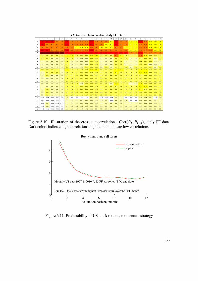
1 2 3 4 5 6 7 8 9 10 11 12 13 14 15 16 17 18 19 20 21 22 23 24 25
1
2
3
4
5
6
7
8
9
10
11
12
13
14
15
16
17
18
19
20
21
22
23
24
25
0.24
0.21
0.19
0.20
0.26
0.09
0.05
0.03
0.03
0.04
0.07
0.05
0.04
0.04
0.03
0.03
0.04
0.04
0.04
0.04
−0.03
−0.02
−0.01
−0.01
−0.02
0.22
0.19
0.20
0.21
0.26
0.09
0.06
0.04
0.04
0.05
0.07
0.06
0.05
0.05
0.05
0.03
0.05
0.06
0.05
0.05
−0.02
−0.01
0.01
0.00
−0.01
0.20
0.19
0.17
0.19
0.25
0.08
0.05
0.04
0.03
0.05
0.06
0.05
0.05
0.04
0.04
0.03
0.04
0.05
0.05
0.04
−0.03
−0.02
−0.00
−0.00
−0.02
0.20
0.19
0.18
0.18
0.26
0.07
0.04
0.04
0.03
0.05
0.06
0.05
0.05
0.05
0.04
0.02
0.04
0.05
0.05
0.04
−0.03
−0.02
−0.00
−0.00
−0.02
0.20
0.19
0.18
0.20
0.26
0.06
0.04
0.03
0.03
0.05
0.04
0.04
0.04
0.04
0.03
0.01
0.03
0.04
0.04
0.04
−0.04
−0.02
−0.01
−0.01
−0.02
0.24
0.22
0.20
0.20
0.24
0.13
0.08
0.06
0.05
0.06
0.11
0.08
0.07
0.06
0.06
0.07
0.08
0.08
0.07
0.06
0.00
0.01
0.02
0.01
0.00
0.20
0.19
0.17
0.18
0.23
0.10
0.06
0.05
0.04
0.05
0.09
0.08
0.07
0.06
0.06
0.07
0.08
0.08
0.07
0.07
−0.00
0.01
0.03
0.02
0.00
0.17
0.16
0.15
0.17
0.22
0.08
0.04
0.03
0.03
0.04
0.08
0.07
0.06
0.05
0.05
0.05
0.07
0.07
0.07
0.06
−0.01
0.00
0.02
0.01
0.00
0.16
0.15
0.14
0.16
0.21
0.07
0.04
0.03
0.02
0.04
0.07
0.06
0.05
0.05
0.05
0.05
0.07
0.07
0.07
0.06
−0.01
0.00
0.02
0.01
0.00
0.16
0.15
0.14
0.16
0.22
0.07
0.04
0.04
0.03
0.05
0.07
0.07
0.06
0.06
0.06
0.05
0.07
0.08
0.08
0.07
−0.00
0.01
0.03
0.02
0.02
0.24
0.21
0.19
0.20
0.24
0.14
0.09
0.07
0.06
0.06
0.13
0.10
0.08
0.06
0.07
0.09
0.09
0.09
0.08
0.07
0.01
0.02
0.03
0.02
0.00
0.20
0.18
0.17
0.19
0.23
0.12
0.07
0.06
0.05
0.06
0.11
0.09
0.08
0.07
0.07
0.08
0.09
0.09
0.08
0.07
0.01
0.02
0.03
0.02
0.01
0.16
0.15
0.14
0.16
0.21
0.08
0.05
0.04
0.03
0.04
0.08
0.07
0.06
0.05
0.06
0.05
0.07
0.07
0.07
0.06
−0.01
0.00
0.02
0.01
0.00
0.15
0.15
0.14
0.16
0.21
0.08
0.05
0.04
0.04
0.05
0.08
0.08
0.07
0.06
0.07
0.06
0.08
0.08
0.08
0.07
−0.00
0.01
0.03
0.02
0.01
0.14
0.14
0.13
0.15
0.21
0.07
0.04
0.03
0.03
0.04
0.07
0.06
0.06
0.05
0.06
0.04
0.06
0.06
0.07
0.06
−0.02
−0.00
0.01
0.01
0.00
0.23
0.21
0.19
0.20
0.23
0.15
0.09
0.07
0.06
0.06
0.14
0.10
0.08
0.07
0.07
0.10
0.10
0.09
0.08
0.08
0.02
0.03
0.04
0.02
0.00
0.18
0.17
0.17
0.18
0.21
0.11
0.08
0.06
0.06
0.06
0.11
0.10
0.09
0.07
0.08
0.08
0.09
0.09
0.09
0.08
0.01
0.02
0.04
0.03
0.01
0.16
0.15
0.15
0.16
0.21
0.09
0.06
0.05
0.05
0.05
0.09
0.08
0.08
0.07
0.07
0.06
0.08
0.08
0.07
0.07
−0.00
0.00
0.02
0.02
0.00
0.13
0.13
0.13
0.14
0.19
0.07
0.04
0.03
0.03
0.04
0.07
0.06
0.06
0.06
0.06
0.04
0.06
0.06
0.07
0.07
−0.02
−0.01
0.01
0.01
0.00
0.13
0.13
0.13
0.14
0.20
0.07
0.04
0.04
0.03
0.05
0.07
0.06
0.06
0.06
0.06
0.04
0.06
0.06
0.07
0.07
−0.02
−0.00
0.02
0.01
0.00
0.21
0.19
0.18
0.19
0.21
0.15
0.10
0.08
0.07
0.07
0.15
0.12
0.10
0.08
0.08
0.12
0.12
0.10
0.09
0.08
0.04
0.04
0.05
0.03
0.01
0.17
0.16
0.16
0.17
0.20
0.12
0.08
0.07
0.06
0.06
0.11
0.11
0.09
0.08
0.08
0.09
0.10
0.10
0.09
0.08
0.02
0.02
0.04
0.03
0.00
0.14
0.15
0.14
0.15
0.19
0.09
0.06
0.05
0.05
0.05
0.10
0.09
0.08
0.07
0.07
0.07
0.09
0.09
0.08
0.08
0.01
0.01
0.03
0.02
0.00
0.12
0.13
0.13
0.14
0.18
0.08
0.05
0.04
0.04
0.05
0.08
0.08
0.08
0.07
0.07
0.06
0.08
0.08
0.08
0.08
−0.00
0.01
0.03
0.02
0.01
0.12
0.12
0.12
0.14
0.18
0.07
0.05
0.05
0.05
0.06
0.08
0.08
0.08
0.07
0.08
0.06
0.08
0.08
0.08
0.09
0.00
0.01
0.04
0.03
0.02
(Auto−)correlation matrix, daily FF returns
Figure 6.10: Illustration of the cross-autocorrelations, Corr.Rt ; Rt�k/, daily FF data.Dark colors indicate high correlations, light colors indicate low correlations.
0 2 4 6 8 10 120
2
4
6
8
Evalutation horizon, months
Buy winners and sell losers
Monthly US data 1957:1−2010:9, 25 FF portfolios (B/M and size)
Buy (sell) the 5 assets with highest (lowest) return over the last month
excess return
alpha
Figure 6.11: Predictability of US stock returns, momentum strategy
133

is weak. The evidence from mutual funds is similar. For them it is typically also foundthat their portfolio weights do not anticipate price movements.
It should be remembered that many analysts also are sales persons: either of a stock(for instance, since the bank is underwriting an offering) or of trading services. It couldwell be that their objective function is quite different from minimizing the squared forecasterrors—or whatever we typically use in order to evaluate their performance. (The numberof litigations in the US after the technology boom/bust should serve as a strong reminderof this.)
6.4.2 Do Security Analysts Overreact?
The paper by Bondt and Thaler (1990) compares the (semi-annual) forecasts (one- andtwo-year time horizons) with actual changes in earnings per share (1976-1984) for severalhundred companies. The paper has regressions like
Actual change D ˛ C ˇ.forecasted change/C residual,
and then studies the estimates of the ˛ and ˇ coefficients. With rational expectations (anda long enough sample), we should have ˛ D 0 (no constant bias in forecasts) and ˇ D 1
(proportionality, for instance no exaggeration).The main findings are as follows. The main result is that 0 < ˇ < 1, so that the
forecasted change tends to be too wild in a systematic way: a forecasted change of 1% is(on average) followed by a less than 1% actual change in the same direction. This meansthat analysts in this sample tended to be too extreme—to exaggerate both positive andnegative news.
6.4.3 High-Frequency Trading Based on Recommendations from Stock Analysts
Barber, Lehavy, McNichols, and Trueman (2001) give a somewhat different picture.They focus on the profitability of a trading strategy based on analyst’s recommendations.They use a huge data set (some 360,000 recommendations, US stocks) for the period1985-1996. They sort stocks in to five portfolios depending on the consensus (average)recommendation—and redo the sorting every day (if a new recommendation is published).They find that such a daily trading strategy gives an annual 4% abnormal return on theportfolio of the most highly recommended stocks, and an annual -5% abnormal return on
134

the least favourably recommended stocks.This strategy requires a lot of trading (a turnover of 400% annually), so trading costs
would typically reduce the abnormal return on the best portfolio to almost zero. A lessfrequent rebalancing (weekly, monthly) gives a very small abnormal return for the beststocks, but still a negative abnormal return for the worst stocks. Chance and Hemler(2001) obtain similar results when studying the investment advise by 30 professional“market timers.”
6.4.4 Economic Experts
Several papers, for instance, Bondt (1991) and Söderlind (2010), have studied whethereconomic experts can predict the broad stock markets. The results suggests that theycannot. For instance, Söderlind (2010) show that the economic experts that participate inthe semi-annual Livingston survey (mostly bank economists) (ii) forecast the S&P worsethan the historical average (recursively estimated), and that their forecasts are stronglycorrelated with recent market data (which in itself, cannot predict future returns).
6.4.5 The Characteristics of Individual Analysts’ Forecasts in Europe
Bolliger (2001) studies the forecast accuracy (earnings per share) of European (13 coun-tries) analysts for the period 1988–1999. In all, some 100,000 forecasts are studied. Itis found that the forecast accuracy is positively related to how many times an analyst hasforecasted that firm and also (surprisingly) to how many firms he/she forecasts. The ac-curacy is negatively related to the number of countries an analyst forecasts and also to thesize of the brokerage house he/she works for.
6.4.6 Bond Rating Agencies versus Stock Analysts
Ederington and Goh (1998) use data on all corporate bond rating changes by Moody’sbetween 1984 and 1990 and the corresponding earnings forecasts (by various stock ana-lysts).
The idea of the paper by Ederington and Goh (1998) is to see if bond ratings driveearnings forecasts (or vice versa), and if they affect stock returns (prices).
1. To see if stock returns are affected by rating changes, they first construct a “normal”
135

return by a market model:
normal stock returnt = ˛ C ˇ � return on stock indext ,
where ˛ and ˇ are estimated on a normal time period (not including the ratingchange). The abnormal return is then calculated as the actual return minus thenormal return. They then study how such abnormal returns behave, on average,around the dates of rating changes. Note that “time” is then measured, individuallyfor each stock, as the distance from the day of rating change. The result is that thereare significant negative abnormal returns following downgrades, but zero abnormalreturns following upgrades.
2. They next turn to the question of whether bond ratings drive earnings forecasts orvice versa. To do that, they first note that there are some predictable patterns inrevisions of earnings forecasts. They therefore fit a simple autoregressive modelof earnings forecasts, and construct a measure of earnings forecast revisions (sur-prises) from the model. They then relate this surprise variable to the bond ratings.In short, the results are the following:
(a) both earnings forecasts and ratings react to the same information, but there isalso a direct effect of rating changes, which differs between downgrades andupgrades.
(b) downgrades: the ratings have a strong negative direct effect on the earningsforecasts; the returns react ever quicker than analysts
(c) upgrades: the ratings have a small positive direct effect on the earnings fore-casts; there is no effect on the returns
A possible reason for why bond ratings could drive earnings forecasts and prices isthat bond rating firms typically have access to more inside information about firms thanstock analysts and investors.
A possible reason for the observed asymmetric response of returns to ratings is thatfirms are quite happy to release positive news, but perhaps more reluctant to release badnews. If so, then the information advantage of bond rating firms may be particularly largeafter bad news. A downgrading would then reveal more new information than an upgrade.
The different reactions of the earnings forecasts and the returns are hard to reconcile.
136

6.4.7 International Differences in Analyst Forecast Properties
Ang and Ciccone (2001) study earnings forecasts for many firms in 42 countries over theperiod 1988 to 1997. Some differences are found across countries: forecasters disagreemore and the forecast errors are larger in countries with low GDP growth, less accountingdisclosure, and less transparent family ownership structure.
However, the most robust finding is that forecasts for firms with losses are special:forecasters disagree more, are more uncertain, and are more overoptimistic about suchfirms.
6.4.8 Analysts and Industries
Boni and Womack (2006) study data on on some 170,000 recommedation for a verylarge number of U.S. companies for the period 1996–2002. Focusing on revisions ofrecommendations, the papers shows that analysts are better at ranking firms within anindustry than ranking industries.
6.5 Technical Analysis
Main reference: Bodie, Kane, and Marcus (2002) 12.2; Neely (1997) (overview, foreignexchange market)Further reading: Murphy (1999) (practical, a believer’s view); The Economist (1993)(overview, the perspective of the early 1990s); Brock, Lakonishok, and LeBaron (1992)(empirical, stock market); Lo, Mamaysky, and Wang (2000) (academic article on returndistributions for “technical portfolios”)
6.5.1 General Idea of Technical Analysis
Technical analysis is typically a data mining exercise which looks for local trends orsystematic non-linear patterns. The basic idea is that markets are not instantaneouslyefficient: prices react somewhat slowly and predictably to news. The logic is essentiallythat an observed price move must be due to some news (exactly which one is not veryimportant) and that old patterns can tell us where the price will move in the near future.This is an attempt to gather more detailed information than that used by the market as awhole. In practice, the technical analysis amounts to plotting different transformations
137

(for instance, a moving average) of prices—and to spot known patterns. This sectionsummarizes some simple trading rules that are used.
6.5.2 Technical Analysis and Local Trends
Many trading rules rely on some kind of local trend which can be thought of as positiveautocorrelation in price movements (also called momentum1).
A moving average rule is to buy if a short moving average (equally weighted or ex-ponentially weighted) goes above a long moving average. The idea is that event signalsa new upward trend. Let S (L) be the lag order of a short (long) moving average, withS < L and let b be a bandwidth (perhaps 0.01). Then, a MA rule for period t could be264buy in t if MAt�1.S/ > MAt�1.L/.1C b/
sell in t if MAt�1.S/ < MAt�1.L/.1 � b/no change otherwise
375 , where (6.21)
MAt�1.S/ D .pt�1 C : : :C pt�S/=S:
The difference between the two moving averages is called an oscillator (or sometimes,moving average convergence divergence2). A version of the moving average oscillator isthe relative strength index3, which is the ratio of average price level on “up” days to theaverage price on “down” days—during the last z (14 perhaps) days.
The trading range break-out rule typically amounts to buying when the price risesabove a previous peak (local maximum). The idea is that a previous peak is a resistance
level in the sense that some investors are willing to sell when the price reaches that value(perhaps because they believe that prices cannot pass this level; clear risk of circularreasoning or self-fulfilling prophecies; round numbers often play the role as resistancelevels). Once this artificial resistance level has been broken, the price can possibly risesubstantially. On the downside, a support level plays the same role: some investors arewilling to buy when the price reaches that value. To implement this, it is common to letthe resistance/support levels be proxied by minimum and maximum values over a data
1In physics, momentum equals the mass times speed.2Yes, the rumour is true: the tribe of chartists is on the verge of developing their very own language.3Not to be confused with relative strength, which typically refers to the ratio of two different asset prices
(for instance, an equity compared to the market).
138
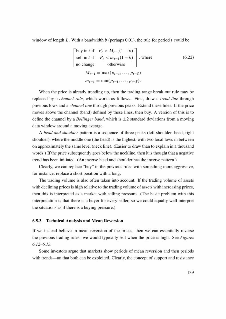
window of length L. With a bandwidth b (perhaps 0.01), the rule for period t could be264buy in t if Pt > Mt�1.1C b/sell in t if Pt < mt�1.1 � b/no change otherwise
375 , where (6.22)
Mt�1 D max.pt�1; : : : ; pt�S/
mt�1 D min.pt�1; : : : ; pt�S/:
When the price is already trending up, then the trading range break-out rule may bereplaced by a channel rule, which works as follows. First, draw a trend line throughprevious lows and a channel line through previous peaks. Extend these lines. If the pricemoves above the channel (band) defined by these lines, then buy. A version of this is todefine the channel by a Bollinger band, which is ˙2 standard deviations from a movingdata window around a moving average.
A head and shoulder pattern is a sequence of three peaks (left shoulder, head, rightshoulder), where the middle one (the head) is the highest, with two local lows in betweenon approximately the same level (neck line). (Easier to draw than to explain in a thousandwords.) If the price subsequently goes below the neckline, then it is thought that a negativetrend has been initiated. (An inverse head and shoulder has the inverse pattern.)
Clearly, we can replace “buy” in the previous rules with something more aggressive,for instance, replace a short position with a long.
The trading volume is also often taken into account. If the trading volume of assetswith declining prices is high relative to the trading volume of assets with increasing prices,then this is interpreted as a market with selling pressure. (The basic problem with thisinterpretation is that there is a buyer for every seller, so we could equally well interpretthe situations as if there is a buying pressure.)
6.5.3 Technical Analysis and Mean Reversion
If we instead believe in mean reversion of the prices, then we can essentially reversethe previous trading rules: we would typically sell when the price is high. See Figures
6.12–6.13.
Some investors argue that markets show periods of mean reversion and then periodswith trends—an that both can be exploited. Clearly, the concept of support and resistance
139

levels (or more generally, a channel) is based on mean reversion between these points. Anew trend is then supposed to be initiated when the price breaks out of this band.
Jan Feb Mar Apr1150
1200
1250
1300
1350
1999
Inverted MA rule, S&P 500
MA(3) and MA(25), bandwidth 0.01
Long MA (−)
Long MA (+)
Short MA
Figure 6.12: Examples of trading rules
6.6 Spurious Regressions and In-Sample Overfit�
References: Ferson, Sarkissian, and Simin (2003), Goyal and Welch (2008), and Camp-bell and Thompson (2008)
6.6.1 Spurious Regressions
Ferson, Sarkissian, and Simin (2003) argue that many prediction equations suffer from“spurious regression” features—and that data mining tends to make things even worse.
Their simulation experiment is based on a simple model where the return predictionsare
rtC1 D ˛ C ıZt C vtC1; (6.23)
where Zt is a regressor (predictor). The true model is that returns follows the process
rtC1 D �CZ�t C utC1; (6.24)
140
−3 −2 −1 0 1 2 30
0.2
0.4
0.6
Distribution of all returns
Return
Mean 0.03
Std 1.18
Daily S&P 500 data 1990:1−2010:9
−3 −2 −1 0 1 2 30
0.2
0.4
0.6
Inverted MA rule: after buy signal
Return
Mean 0.06
Std 1.72
−3 −2 −1 0 1 2 30
0.2
0.4
0.6
Inverted MA rule: after neutral signal
Return
Mean 0.04
Std 0.93
−3 −2 −1 0 1 2 30
0.2
0.4
0.6
Inverted MA rule: after sell signal
Return
Mean 0.00
Std 0.92
Figure 6.13: Examples of trading rules
where the residual is white noise. In this equation, Z�t represents movements in expectedreturns. The predictors follow a diagonal VAR(1)"
Zt
Z�t
#D"� 0
0 ��
#"Zt�1
Z�t�1
#C""t
"�t
#, with Cov
""t
"�t
#!D ˙: (6.25)
In the case of a “pure spurious regression,” the innovations to the predictors are uncor-related (˙ is diagonal). In this case, ı ought to be zero—and their simulations show thatthe estimates are almost unbiased. Instead, there is a problem with the standard deviationof Oı. If �� is high, then the returns will be autocorrelated.
Under the null hypothesis of ı D 0, this autocorrelation is loaded onto the residuals.For that reason, the simulations use a Newey-West estimator of the covariance matrix(with an automatic choice of lag order). This should, ideally, solve the problem with theinference—but the simulations show that it doesn’t: whenZ�t is very autocorrelated (0.95
141

1990 1995 2000 2005 2010
2
4
6
Hold index if MA(3)>MA(25)
Year
SMI
Rule
1990 1995 2000 2005 2010
2
4
6
Hold index if Pt > max(P
t−1,...,P
t−5)
Year
1990 1995 2000 2005 2010
2
4
6
Hold index if Pt/P
t−7 > 1
Year
Daily SMI data
Weekly rebalancing: hold index or riskfree
Figure 6.14: Examples of trading rules
or higher) and reasonably important (so an R2 from running (6.24), if we could, would be0.05 or higher), then the 5% critical value (for a t-test of the hypothesis ı D 0) would be2.7 (to be compared with the nominal value of 1.96). Since the point estimates are almostunbiased, the interpretation is that the standard deviations are underestimated. In contrast,with low autocorrelation and/or low importance of Z�t , the standard deviations are muchmore in line with nominal values.
See Figures 6.15–6.16 for an illustration. They show that we need a combination of anautocorrelated residual and an autocorrelated regressor to create a problem for the usualLS formula for the standard deviation of a slope coefficient. When the autocorrelation isvery high, even the Newey-West estimator is likely to underestimate the true uncertainty.
To study the interaction between spurious regressions and data mining, Ferson, Sarkissian,and Simin (2003) let Zt be chosen from a vector of L possible predictors—which all are
142

−0.5 0 0.5
−0.5
0
0.5
Autocorrelation of xtu
t
ρ
κ = −0.9
κ = 0
κ = 0.9
Model: yt = 0.9x
t + ε
t,
where εt = ρε
t−1 + u
t,
where ut is iid N(0,h) such that Std(ε
t) = 1, and
xt = κx
t−1 + η
t
bLS
is the LS estimate of b in
yt = a + bx
t + u
t
Figure 6.15: Autocorrelation of xtut when ut has autocorrelation �
−0.5 0 0.50
0.05
0.1
Std of LS under autocorrelation, κ = −0.9
ρ
σ2(X’X)
−1
Newey−West Simulated
−0.5 0 0.50
0.05
0.1
Std of LS under autocorrelation, κ = 0
ρ
−0.5 0 0.50
0.05
0.1
Std of LS under autocorrelation, κ = 0.9
ρ
Figure 6.16: Variance of OLS estimator, autocorrelated errors
143

generated by a diagonal VAR(1) system as in (6.25) with uncorrelated errors. It is assumedthat the researcher chooses Zt by running L regressions, and then picks the one with thehighest R2. When �� D 0:15 and the researcher chooses between L D 10 predictors,the simulated 5% critical value is 3.5. Since this does not depend on the importance ofZ�t , it is interpreted as a typical feature of “data mining,” which is bad enough. With theautocorrelation is 0.95, then the importance of Z�t becomes important—“spurious regres-sions” interact with the data mining to create extremely high simulated critical values. Apossible explanation is that the data mining exercise is likely to pick out the most auto-correlated predictor, and that a highly autocorrelated predictor exacerbates the spuriousregression problem.
6.6.2 In-Sample versus Out-of-Sample Forecasting
Goyal and Welch (2008) find that the evidence of predictability of equity returns dis-appears when out-of-sample forecasts are considered. Campbell and Thompson (2008)claim that there is still some out-of-sample predictability, provided we put restrictions onthe estimated models.
Campbell and Thompson (2008) first report that only few variables (earnings priceratio, T-bill rate and the inflation rate) have significant predictive power for one-monthstock returns in the full sample (1871–2003 or early 1920s–2003, depending on predictor).
To gauge the out-of-sample predictability, they estimate the prediction equation usingdata up to and including t � 1, and then make a forecast for period t . The forecastingperformance of the equation is then compared with using the historical average as thepredictor. Notice that this historical average is also estimated on data up to an includingt � 1, so it changes over time. Effectively, they are comparing the forecast performanceof two models estimated in a recursive way (long and longer sample): one model has justan intercept, the other has also a predictor. The comparison is done in terms of the RMSEand an “out-of-sample R2”
R2OS D 1 �XT
tDs.rt � Ort/2 =
XT
tDs.rt � Nrt/2 ; (6.26)
where s is the first period with an out-of-sample forecast, Ort is the forecast based on theprediction model (estimated on data up to and including t � 1) and Nrt is the historicalaverage (also estimated on data up to and including t � 1).
144

The evidence shows that the out-of-sample forecasting performance is very weak—asclaimed by Goyal and Welch (2008).
It is argued that forecasting equations can easily give strange results when they areestimated on a small data set (as they are early in the sample). They therefore try differentrestrictions: setting the slope coefficient to zero whenever the sign is “wrong,” settingthe prediction (or the historical average) to zero whenever the value is negative. Thisimproves the results a bit—although the predictive performance is still weak.
See Figure 6.17 for an illustration.
100 150 200 250 300 3500.16
0.17
0.18
0.19
0.2
Length of data window, months
RMSE, E/P regression vs MA
MA
Regression
100 150 200 250 300 3500.16
0.17
0.18
0.19
0.2
RMSE, max(E/P regression,0) vs MA
Length of data window, months
US stock 1−year returns 1926:1−2010:4
Predictions made for 1957:1−2010:4
Estimation is done on moving data window; forecasts made out of sample
In−sample RMSE: 0.17
Figure 6.17: Predictability of US stock returns, in-sample and out-of-sample
6.7 Empirical U.S. Evidence on Stock Return Predictability
The two most common methods for investigating the predictability of stock returns areto calculate autocorrelations and to construct simple dynamic portfolios and see if theyoutperform passive portfolios. The dynamic portfolio could, for instance, be a simplefilter rule that calls for rebalancing once a month by buying (selling) assets which haveincreased (decreased) by more than x% the last month. If this portfolio outperforms apassive portfolio, then this is evidence of some positive autocorrelation (“momentum”)on a one-month horizon. The following points summarize some evidence which seems to
145

hold for both returns and returns in excess of a riskfree rate (an interest rate).
1. The empirical evidence suggests some, but weak, positive autocorrelation in short
horizon returns (one day up to a month) — probably too little to trade on. Theautocorrelation is stronger for small than for large firms (perhaps no autocorrela-tion at all for weekly or longer returns in large firms). This implies that equallyweighted stock indices have higher autocorrelations than value-weighted indices.(See Campbell, Lo, and MacKinlay (1997) Table 2.4.)
2. Stock indices have more positive autocorrelation than (most) individual stocks:there must be fairly strong cross-autocorrelations across individual stocks. (SeeCampbell, Lo, and MacKinlay (1997) Tables 2.7 and 2.8.)
3. There seems to be negative autocorrelation of multi-year stock returns, for instancein 5-year US returns for 1926-1985. It is unclear what drives this result, how-ever. It could well be an artifact of just a few extreme episodes (Great Depression).Moreover, the estimates are very uncertain as there are very few (non-overlapping)multi-year returns even in a long sample—the results could be just a fluke.
4. The aggregate stock market returns, that is, a return on a value-weighted stockindex, seems to be forecastable on the medium horizon by various information
variables. In particular, future stock returns seem to be predictable by the currentdividend-price ratio and earnings-price ratio (positively, one to several years), orby the interest rate changes (negatively, up to a year). For instance, the coefficientof determination (usually denoted R2, but not to be confused with the return usedabove) for predicting the two-year return on the US stock market by the currentdividend-price ratio is around 0.3 for the 1952-1994 sample. (See Campbell, Lo,and MacKinlay (1997) Tables 7.1-2.) This evidence suggests that expected returnsmay very well be time-varying and correlated with the business cycle.
5. Even if short-run returns, RtC1, are fairly hard to forecast, it is often fairly easyto forecast volatility as measured by jRtC1j or R2tC1 (for instance, using ARCHor GARCH models). For an example, see Bodie, Kane, and Marcus (2002) Fig-ure 13.7. This could possibly be used for dynamic trading strategies on options(which directly price volatility). For instance, buying both a call and a put option (a“straddle” or a “strangle”), is a bet on a large price movement (in any direction).
146

6. It is sometimes found that stock prices behave differently in periods with highvolatility than in more normal periods. Granger (1992) reports that the forecast-ing performance is sometimes improved by using different forecasting models forthese two regimes. A simple and straightforward way to estimate a model for peri-ods of normal volatility is to simply throw out data for volatile periods (and otherexceptional events).
7. It is important to assess forecasting models in terms of their out-of-sample forecast-ing performance. Too many models seem to fit data in-sample, but most of themfail in out-of-sample tests. Forecasting models are of no use if they cannot forecast.
8. There are also a number of strange patterns (“anomalies”) like the small-firms-in-January effect (high returns on these in the first part of January) and the book-to-market effect (high returns on firms with high book/market value of the firm’sequity).
Bibliography
Ang, J. S., and S. J. Ciccone, 2001, “International differences in analyst forecast proper-ties,” mimeo, Florida State University.
Barber, B., R. Lehavy, M. McNichols, and B. Trueman, 2001, “Can investors profit fromthe prophets? Security analyst recommendations and stock returns,” Journal of Fi-
nance, 56, 531–563.
Bodie, Z., A. Kane, and A. J. Marcus, 2002, Investments, McGraw-Hill/Irwin, Boston,5th edn.
Bolliger, G., 2001, “The characteristics of individual analysts’ forecasts in Europe,”mimeo, University of Neuchatel.
Bondt, W. F. M. D., 1991, “What do economists know about the stock market?,” Journal
of Portfolio Management, 17, 84–91.
Bondt, W. F. M. D., and R. H. Thaler, 1990, “Do security analysts overreact?,” American
Economic Review, 80, 52–57.
147

Boni, L., and K. L. Womack, 2006, “Analysts, industries, and price momentum,” Journal
of Financial and Quantitative Analysis, 41, 85–109.
Brock, W., J. Lakonishok, and B. LeBaron, 1992, “Simple technical trading rules and thestochastic properties of stock returns,” Journal of Finance, 47, 1731–1764.
Brockwell, P. J., and R. A. Davis, 1991, Time series: theory and methods, Springer Verlag,New York, second edn.
Campbell, J. Y., A. W. Lo, and A. C. MacKinlay, 1997, The econometrics of financial
markets, Princeton University Press, Princeton, New Jersey.
Campbell, J. Y., and S. B. Thompson, 2008, “Predicting the equity premium out of sam-ple: can anything beat the historical average,” Review of Financial Studies, 21, 1509–1531.
Chance, D. M., and M. L. Hemler, 2001, “The performance of professional market timers:daily evidence from executed strategies,” Journal of Financial Economics, 62, 377–411.
Cochrane, J. H., 2001, Asset pricing, Princeton University Press, Princeton, New Jersey.
Cuthbertson, K., 1996, Quantitative financial economics, Wiley, Chichester, England.
Ederington, L. H., and J. C. Goh, 1998, “Bond rating agencies and stock analysts: whoknows what when?,” Journal of Financial and Quantitative Analysis, 33, 569–585.
Elton, E. J., M. J. Gruber, S. J. Brown, and W. N. Goetzmann, 2010, Modern portfolio
theory and investment analysis, John Wiley and Sons, 8th edn.
Ferson, W. E., S. Sarkissian, and T. T. Simin, 2003, “Spurious regressions in financialeconomics,” Journal of Finance, 57, 1393–1413.
Goyal, A., and I. Welch, 2008, “A comprehensive look at the empirical performance ofequity premium prediction,” Review of Financial Studies 2008, 21, 1455–1508.
Granger, C. W. J., 1992, “Forecasting stock market prices: lessons for forecasters,” Inter-
national Journal of Forecasting, 8, 3–13.
148
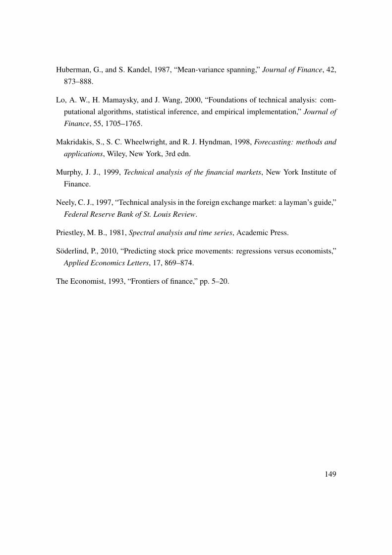
Huberman, G., and S. Kandel, 1987, “Mean-variance spanning,” Journal of Finance, 42,873–888.
Lo, A. W., H. Mamaysky, and J. Wang, 2000, “Foundations of technical analysis: com-putational algorithms, statistical inference, and empirical implementation,” Journal of
Finance, 55, 1705–1765.
Makridakis, S., S. C. Wheelwright, and R. J. Hyndman, 1998, Forecasting: methods and
applications, Wiley, New York, 3rd edn.
Murphy, J. J., 1999, Technical analysis of the financial markets, New York Institute ofFinance.
Neely, C. J., 1997, “Technical analysis in the foreign exchange market: a layman’s guide,”Federal Reserve Bank of St. Louis Review.
Priestley, M. B., 1981, Spectral analysis and time series, Academic Press.
Söderlind, P., 2010, “Predicting stock price movements: regressions versus economists,”Applied Economics Letters, 17, 869–874.
The Economist, 1993, “Frontiers of finance,” pp. 5–20.
149

.D..3
7 Maximum Likelihood Estimation
Reference: Verbeek (2008) 2 and 4More advanced material is denoted by a star (�). It is not required reading.
7.1 Maximum Likelihood
A different route to create a estimate is to maximize the likelihood function.To understand the principle of maximum likelihood estimation, consider the following
examples.
7.1.1 Example: Estimating the Mean with ML
Suppose we know xt � N.�; �2/, but we don’t know the value of � (for now, assumewe know the variance). Since xt is a random variable, there is a probability of everyobservation and the density function of xt is
L D pdf .xt/ D 1p2��2
exp��12
.xt � �/2�2
�; (7.1)
whereL stands for “likelihood.” The basic idea of maximum likelihood estimation (MLE)is to pick model parameters to make the observed data have the highest possible proba-bility. Here this gives O� D xt . This is the maximum likelihood estimator in this example.
What if there are T observations, x1; x2,...xT ? In the simplest case where xi and xjare independent, then the joint pdf is just the product of the individual pdfs (for instance,pdf.xi ; xj / D pdf.xi/ pdf.xj /) so
L D pdf .x1/ � pdf .x2/ � ::: � pdf .xT / (7.2)
D .2��2/�T=2 exp��12
�.x1 � �/2
�2C .x2 � �/2
�2C :::C .xT � �/2
�2
��(7.3)
150

Take logs (log likelihood)
lnL D �T2
ln.2��2/ � 1
2�2
�.x1 � �/2 C .x2 � �/2 C :::C .xT � �/2
�: (7.4)
The derivative with respect to � is
@ lnL@�
D 1
�2Œ.x1 � �/C .x2 � �/C :::C .xT � �/� : (7.5)
To maximize the likelihood function find the value of O� that makes @ lnL=@� D 0, whichis the usual sample average
O� D .x1 C x2 C :::C xT / =T: (7.6)
Remark 7.1 (Coding the log likelihood function) Many software packages want just the
likelihood contribution of data point t (not the ful) lnLt D �12 ln.2��2/� 12�2
.xt � �/2.
7.1.2 Example: Estimating the Variance with ML�
To estimate the variance, use (7.4) and find the value �2 that makes @ lnL=@�2 D 0
0 D @ lnL@�2
D �T2
1
2��22� C 1
2.�2/2
�.x1 � �/2 C .x2 � �/2 C :::C .xT � �/2
�; (7.7)
soO�2 D 1
T
�.x1 � �/2 C .x2 � �/2 C :::C .xT � �/2
�: (7.8)
Notice that we divide by T , not by T � 1, so O�2 must be biased, but the bias disappearsas T !1
7.1.3 MLE of a Regression
To apply this idea to a (multiple) regression model
yt D ˇ0xt C ut ; (7.9)
151

we could assume that ut is iid N.0; �2/. The probability density function of ut is
pdf .ut/ D 1p2��2
exp��12u2t =�
2
�: (7.10)
Since the errors are independent, we get the joint pdf of the u1; u2; : : : ; uT by multiplyingthe marginal pdfs of each of the errors
L D pdf .u1/ � pdf .u2/ � ::: � pdf .uT /
D .2��2/�T=2 exp��12
�u21�2C u22�2C :::C u2T
�2
��: (7.11)
Substitute yt � ˇ0xt for ut and take logs to get the log likelihood function of the sample
lnL DXT
tD1lnLt , where (7.12)
lnLt D �12
ln .2�/ � 12
ln.�2/ � 12
�yt � ˇ0xt
�2=�2: (7.13)
Suppose (for simplicity) that we happen to know the value of �2. It is then clear thatthis likelihood function is maximized by minimizing the last term, which is proportionalto the sum of squared errors: LS is ML when the errors are iid normally distributed (butonly then). (This holds also when we do not know the value of �2—just slightly messierto show it.) See Figure 7.1.
Maximum likelihood estimators have very nice properties, provided the basic distri-butional assumptions are correct, that is, if we maximize the right likelihood function.In that case, MLE is typically the most efficient/precise estimators (at least in very largesamples). ML also provides a coherent framework for testing hypotheses (including theWald, LM, and LR tests).
Example 7.2 Consider the regression model yi D ˇ2xiCui , where we (happen to) know
that ui � N.0; 1/.Suppose we have the following datahy1 y2 y3
iDh�1:5 �0:6 2:1
iand
hx1 x2 x3
iDh�1 0 1
i:
152

Suppose .y1; x1/ D .�1:5;�1/. Try different values of ˇ2 on observation 1
ˇ2 u1 Density function value of u11:6 �1:5 � 1:6 � .�1/ D 0:1 0:40
1:8 �1:5 � 1:8 � .�1/ D 0:3 0:38
2:0 �1:5 � 2:0 � .�1/ D 0:5 0:35
Observation 1 favours ˇ D 1:6; see Figure 7.2. Do the same for observations 2 and 3:
ˇ2 u2 Density function value of u21:6 �0:6 � 1:6 � 0 D �0:6 0:33
1:8 �0:6 � 1:8 � 0 D �0:6 0:33
2:0 �0:6 � 2:0 � 0 D �0:6 0:33
ˇ2 u3 Density function value of u31:6 2:1 � 1:6 � 1 D 0:5 0:35
1:8 2:1 � 1:8 � 1 D 0:3 0:38
2:0 2:1 � 2:0 � 1 D 0:1 0:40
To sum up, observation 1 favours ˇ D 1:6, observation 2 is neutral, and observation 3
favours ˇ D 2. The estimate is a “compromise” that maximixes the joint density (the
product of the individual densities since the ui are independent)
ˇ2 pdf.u1/ � pdf.u2/ � pdf.u3/1:6 0:40 � 0:33 � 0:35 � 0:0471:8 0:38 � 0:33 � 0:38 � 0:0482:0 0:35 � 0:33 � 0:40 � 0:047
so 1:8 has the highest likelihood value of these three alternatives (it is actually the opti-
mum). See Figure 7.2.
Example 7.3 Consider the simple regression where we happen to know that the intercept
is zero, yt D ˇ1xt C ut . Suppose we have the following datahy1 y2 y3
iDh�1:5 �0:6 2:1
iand
hx1 x2 x3
iDh�1 0 1
i:
153

Suppose ˇ2 D 2, then we get the following values for ut D yt � 2xt and its square264�1:5 � 2 � .�1/�0:6 � 2 � 02:1 � 2 � 1
375 D264 0:5
�0:60:1
375 with the square
2640:250:36
0:01
375 with sum 0:62:
Now, suppose instead that ˇ2 D 1:8, then we get264�1:5 � 1:8 � .�1/�0:6 � 1:8 � 02:1 � 1:8 � 1
375 D264 0:3
�0:60:3
375 with the square
2640:090:36
0:09
375 with sum 0:54:
The latter choice of ˇ2 will certainly give a larger value of the likelihood function (it is
actually the optimum). See Figure 7.1.
7.1.4 MLE of a Regression with GARCH(1,1) Errors
Consider a regression model where the residuals are uncorrelated across time, but havetime-varying volatility
yt D b0xt C ut ; where ut is N.0; �2t /: (7.14)
The variance follows the GARCH(1,1) process
�2t D ! C ˛u2t�1 C ˇ�2t�1: (7.15)
(It is assumed that ! > 0; ˛; ˇ � 0; and ˛ C ˇ < 1.)To estimate this model (that is, the parameters in (b; !; ˛; ˇ), we could use a numerical
optimization routine to maximize the log likelihood function
lnL DTXtD1
Lt , where Lt D �12
ln .2�/ � 12
ln �2t �1
2
u2t�2t: (7.16)
This means, in effect, that the optimization routine searches for the values of (b; !; ˛; ˇ)that makes the value of the log likelihood function as large as possible.
Remark 7.4 To perform the estimation, we also need to supply the optimization routine
with a starting value for �21 and make sure that the restrictions on the GARCH parameters
154

−1 −0.5 0 0.5 1
−2
−1
0
1
2
OLS, y = b0 + b
1x + u, b
0=0
Data
fitted
x
y
y: −1.5 −0.6 2.1
x: −1.0 0.0 1.0
b1: 1.8 (OLS)
0 1 2 3 40
5
10Sum of squared errors
b1
0 1 2 3 4−15
−10
−5
0Log likelihood
b1
Figure 7.1: Example of OLS and ML estimation
are fulfilled.
7.2 Key Properties of MLE
No general results on small-sample properties of MLE: can be biased or not...MLE have very nice asymptotic (large-sample) properties, provided we maximize the
right likelihood function. If so, then
1. MLE is consistent (Pr.j O � ˇj > any number/ gets very small as T gets large)
2. MLE is the most efficient/precise estimator, at least asymptotically (efficient =smallest variance)
155
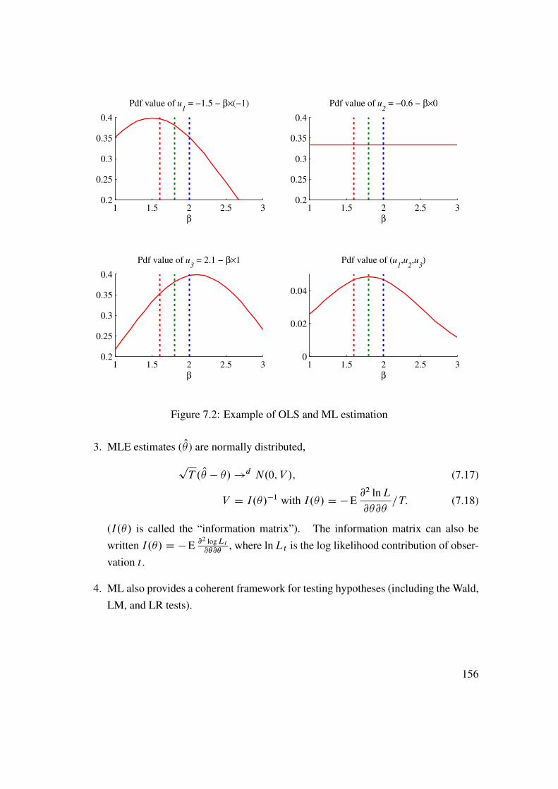
1 1.5 2 2.5 30.2
0.25
0.3
0.35
0.4
Pdf value of u1 = −1.5 − β×(−1)
β1 1.5 2 2.5 3
0.2
0.25
0.3
0.35
0.4
Pdf value of u2 = −0.6 − β×0
β
1 1.5 2 2.5 30.2
0.25
0.3
0.35
0.4
Pdf value of u3 = 2.1 − β×1
β1 1.5 2 2.5 3
0
0.02
0.04
Pdf value of (u1,u
2,u
3)
β
Figure 7.2: Example of OLS and ML estimation
3. MLE estimates ( O� ) are normally distributed,
pT . O� � �/!d N.0; V /; (7.17)
V D I.�/�1 with I.�/ D �E@2 lnL@�@�
=T: (7.18)
(I.�/ is called the “information matrix”). The information matrix can also bewritten I.�/ D �E @2 logLt
@�@�, where lnLt is the log likelihood contribution of obser-
vation t .
4. ML also provides a coherent framework for testing hypotheses (including the Wald,LM, and LR tests).
156

7.2.1 Example of the Information Matrix
Differentiate (7.5) (and assume we know �2) to get
@2 lnL@�@�
D � T�2: (7.19)
The information matrix is
I.�/ D �E@2 lnL@�@�
=T D 1
�2; (7.20)
which we combine with (7.17)–(7.18) to get
pT . O� � �/!d N.0; �2/ or O�!d N.�; �2=T /: (7.21)
This is the standard expression for the distribution of a sample average.
7.3 Three Test Principles
Wald test. Estimate � with MLE, check if O� � �H0 is too large. Example: t-test and F-testLikelihood ratio test. Estimate � with MLE as usual, estimate again by imposing the
H0 restrictions, test if lnL. O�/ � lnL.“ O� with H0 restrictions”/ D 0. Example: comparethe R2 from a model without and with a restriction that some coefficient equals 1/3
Lagrange multiplier test. Estimate � under theH0 restrictions, check if @ lnL=@� D 0for unconstrained model is true when evaluated at “ O� with H0 restrictions”
7.4 QMLE�
A MLE based on the wrong likelihood function (distribution) may still be useful.Suppose we use the likelihood function L and get estimates O� by
@ lnL@�D 0 (7.22)
If L is wrong, then we are maximizing the wrong thing. With some luck, we still getreasonable (concistent) estimates.
Example 7.5 (LS and QMLE) In a linear regression, yt D x0tˇ C "t , the first order
condition for MLE based on the assumption that "t � N.0; �2/ is˙TtD1.yt�x0t O/xt D 0.
157

This has an expected value of zero (at the true parameters), even if the shocks have a, say,
t22 distribution (which would define the correct likelihood function).
The example suggests that if
E@ lnL@�D 0; (7.23)
then the estimates are still consistent. We are doing quasi-MLE (or pseudo-MLE).With QMLE,
pT . O� � �/!d N.0; V /, but
V D I.�/�1 E�@ lnLt@�
�@ lnLt@�
�0�I.�/�1 (7.24)
Practical implication: this is perhaps a “safer” way of constructing tests—since it isless restrictive than assuming that we have the exactly correct likelihood function.
Bibliography
Verbeek, M., 2008, A guide to modern econometrics, Wiley, Chichester, 3rd edn.
158

.D..3
8 ARCH and GARCH
Reference: Bodie, Kane, and Marcus (2005) 13.4Reference (advanced): Taylor (2005) 8–9; Verbeek (2004) 8; Campbell, Lo, and MacKin-lay (1997) 12; Franses and van Dijk (2000)
8.1 Heteroskedasticity
8.1.1 Descriptive Statistics of Heteroskedasticity
Time-variation in volatility (heteroskedasticity) is a common feature of macroeconomicand financial data.
The perhaps most straightforward way to gauge heteroskedasticity is to estimate atime-series of variances on “rolling samples.” For a zero-mean variable, ut , this couldmean
�2t D .u2t�1 C u2t�2 C : : :C u2t�q/=q; (8.1)
where the latest q observations are used. Notice that �2t depends on lagged information,and could therefore be thought of as the prediction (made in t � 1) of the volatility in t .
See Figure 8.1 for an example.Unfortunately, this method can produce quite abrupt changes in the estimate. An
alternative is to apply an exponential moving average (EMA) estimator of volatility, whichuses all data points since the beginning of the sample—but where recent observationscarry larger weights. The weight for lag s is .1 � �/�s where 0 < � < 1, so
�2t D .1 � �/.u2t�1 C �u2t�2 C �2u2t�3 C : : :/; (8.2)
which can also be calculated in a recursive fashion as
�2t D .1 � �/u2t�1 C ��2t�1: (8.3)
The initial value (before the sample) could be assumed to be zero or (perhaps better) the
159

Mon Tue Wed Thu Fri0.03
0.035
0.04
Standard deviation, different weekdays
0 6 12 18
0.02
0.03
0.04
0.05
Standard deviation, different hours
Hour
5−minute data on EUR/USD changes, 1998:1−2010:8
Sample size: 951526
Figure 8.1: Standard deviation for EUR/USD exchange rate changes
(1) (2) (3)
lagged RV 0.76 0.27(10.46) (2.08)
lagged VIX 0.91 0.63(11.90) (6.65)
constant 3.80 -2.70 -1.22(3.88) (-2.01) (-1.51)
R2 0.58 0.62 0.64obs 5139.00 5159.00 5139.00
Table 8.1: Regression of 22-day realized S&P return volatility 1990:1-2010:9. All dailyobservations are used, so the residuals are likely to be autocorrelated. Numbers in paren-theses are t-stats, based on Newey-West with 30 lags.
unconditional variance in a historical sample.This methods is commonly used by practitioners. For instance, the RISK Metrics
uses this method with � D 0:94 for use on daily data. Alternatively, � can be chosen tominimize some criterion function like ˙T
tD1.u2t � �2t /2.
See Figure 8.2 for an example.
160
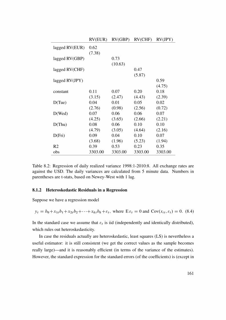
RV(EUR) RV(GBP) RV(CHF) RV(JPY)
lagged RV(EUR) 0.62(7.38)
lagged RV(GBP) 0.73(10.63)
lagged RV(CHF) 0.47(5.87)
lagged RV(JPY) 0.59(4.75)
constant 0.11 0.07 0.20 0.18(3.15) (2.47) (4.43) (2.39)
D(Tue) 0.04 0.01 0.05 0.02(2.76) (0.98) (2.56) (0.72)
D(Wed) 0.07 0.06 0.06 0.07(4.25) (3.65) (2.66) (2.21)
D(Thu) 0.08 0.06 0.10 0.10(4.79) (3.05) (4.64) (2.16)
D(Fri) 0.09 0.04 0.10 0.07(3.68) (1.96) (5.23) (1.94)
R2 0.39 0.53 0.23 0.35obs 3303.00 3303.00 3303.00 3303.00
Table 8.2: Regression of daily realized variance 1998:1-2010:8. All exchange rates areagainst the USD. The daily variances are calculated from 5 minute data. Numbers inparentheses are t-stats, based on Newey-West with 1 lag.
8.1.2 Heteroskedastic Residuals in a Regression
Suppose we have a regression model
yt D b0Cx1tb1Cx2tb2C� � �CxktbkC"t ; where E "t D 0 and Cov.xit ; "t/ D 0: (8.4)
In the standard case we assume that "t is iid (independently and identically distributed),which rules out heteroskedasticity.
In case the residuals actually are heteroskedastic, least squares (LS) is nevertheless auseful estimator: it is still consistent (we get the correct values as the sample becomesreally large)—and it is reasonably efficient (in terms of the variance of the estimates).However, the standard expression for the standard errors (of the coefficients) is (except in
161

1980 1990 2000 20100
10
20
30
40
50GARCH std, annualized
1980 1990 2000 20100
10
20
30
40
50
EMA std, annualized, λ = 0.99
S&P 500 (daily) 1954:1−2010:12
AR(1) of excess returns
with GARCH(1,1) errors
AR(1) coef: 0.10
ARCH&GARCH coefs: 0.08 0.92
1980 1990 2000 20100
10
20
30
40
50
EMA std, annualized, λ = 0.9
Figure 8.2: Conditional standard deviation, estimated by GARCH(1,1) model
1995 2000 2005 20100
20
40
60Std of DAX, GARCH(1,1)
Std
Daily DAX returns 1991:1−2010:9
model: σ2
t = α
0 + α
1u
2
t−1 + β
1σ
2
t−1, u
t is N(0,σ
2
t)
ut is the de−meaned return
α0
α1
β1
Coef
0.032
0.086
0.898
Std err
0.005
0.008
0.009
Figure 8.3: Results for a univariate GARCH model
a special case, see below) not correct. This is illustrated in Figure 8.4.There are two ways to handle this problem. First, we could use some other estimation
method than LS that incorporates the structure of the heteroskedasticity. For instance,
162
combining the regression model (8.4) with an ARCH structure of the residuals—and es-timate the whole thing with maximum likelihood (MLE) is one way. As a by-productwe get the correct standard errors provided, of course, the assumed distribution is cor-rect. Second, we could stick to OLS, but use another expression for the variance of thecoefficients: a “heteroskedasticity consistent covariance matrix,” among which “White’scovariance matrix” is the most common.
To test for heteroskedasticity, we can use White’s test of heteroskedasticity. The nullhypothesis is homoskedasticity, and the alternative hypothesis is the kind of heteroskedas-ticity which can be explained by the levels, squares, and cross products of the regressors—clearly a special form of heteroskedasticity. The reason for this specification is that if thesquared residual is uncorrelated with wt , then the usual LS covariance matrix applies—even if the residuals have some other sort of heteroskedasticity (this is the special casementioned before).
To implement White’s test, let wi be the squares and cross products of the regressors.For instance, if the regressors include .1; x1t ; x2t/ thenwt is the vector (1; x1t ; x2t ; x21t ; x1tx2t ; x
22t )—
since .1; x1t ; x2t/� 1 is .1; x1t ; x2t/ and 1� 1 D 1. The test is then to run a regression ofsquared fitted residuals on wt
O"2t D w0t C vi ; (8.5)
and to test if all the slope coefficients (not the intercept) in are zero. (This can be donebe using the fact that TR2 � �2p, p D dim.wi/ � 1:)
8.1.3 Autoregressive Conditional Heteroskedasticity (ARCH)
Autoregressive heteroskedasticity is a special form of heteroskedasticity—and it is oftenfound in financial data which shows volatility clustering (calm spells, followed by volatilespells, followed by...).
To test for ARCH features, Engle’s test of ARCH is perhaps the most straightforward.It amounts to running an AR(q) regression of the squared zero-mean variable (here de-noted ut )
u2t D ! C a1u2t�1 C : : :C aqu2t�q C vt ; (8.6)
Under the null hypothesis of no ARCH effects, all slope coefficients are zero and theR2 of the regression is zero. (This can be tested by noting that, under the null hypothesis,TR2 � �2q.) This test can also be applied to the fitted residuals from a regression like (8.4).
163

−0.5 −0.4 −0.3 −0.2 −0.1 0 0.1 0.2 0.30
0.01
0.02
0.03
0.04
0.05
0.06
0.07
0.08
0.09
0.1Std of LS estimator under heteroskedasticity
α
Model: yt = 0.9x
t + ε
t,
where εt ∼ N(0,h
t), with h
t = 0.5exp(αx
t
2)
bLS
is the LS estimate of b in
yt = a + bx
t + u
t
σ2(X’X)
−1
White’s
Simulated
Figure 8.4: Variance of OLS estimator, heteroskedastic errors
However, in this case, it is not obvious that ARCH effects make the standard expressionfor the LS covariance matrix invalid—this is tested by White’s test as in (8.5).
8.2 ARCH Models
This section discusses the Autoregressive Conditional Heteroskedasticity (ARCH) model.It is a model of how volatility depends on recent volatility.
There are two basic reasons for being interested in an ARCH model. First, if resid-uals of the regression model (8.4) have ARCH features, then an ARCH model (that is, aspecification of exactly how the ARCH features are generated) can help us estimate the re-gression model by maximum likelihood. Second, we may be interested in understandingthe ARCH features more carefully, for instance, as an input in a portfolio choice processor option pricing.
164
8.2.1 Properties of ARCH(1)
In the ARCH(1) model the residual in the regression equation (8.4), or some other zero-mean variable, can be written
ut � N.0; �2t /, with (8.7)
�2t D ! C ˛u2t�1, with ! > 0 and 0 � ˛ < 1: (8.8)
The non-negativity restrictions on ! and ˛ are needed in order to guarantee �2t > 0. Theupper bound ˛ < 1 is needed in order to make the conditional variance stationary (morelater).
It is clear that the unconditional distribution of ut is non-normal. While the condi-tional distribution of ut is N.0; �2t /, the unconditional distribution of ut is a mixture ofnormal distributions with different (and random) variances. It can be shown that the resultis a distribution which has fatter tails than a normal distribution with the same variance(excess kurtosis)—which is a common feature of financial data.
It is straightforward to show that the ARCH(1) model implies that we in period t canforecast the future conditional variance in t C s as (since �2tC1 is known in t . )
Et �2tCs D N�2 C ˛s�1��2tC1 � N�2
�, with N�2 D !
1 � ˛ ; (8.9)
where N�2 is the unconditional variance. The conditional volatility behaves like an AR(1),and 0 � ˛ < 1 is necessary to keep it positive and stationary.
See Figure 8.5 for an illustration of the fitted volatilies.
8.2.2 Estimation of the ARCH(1) Model
The most common way to estimate the model is to assume that vt �iid N.0; 1/ and toset up the likelihood function. The log likelihood is easily found, since the model isconditionally Gaussian. It is
lnL DTXtD1
Lt , where Lt D �12
ln .2�/ � 12
ln �2t �1
2
u2t�2t: (8.10)
The estimates are found by maximizing the likelihood function (by choosing the parame-ters). This is done by a numerical optimization routine, which should preferably impose
165

1980 1990 2000 20100
10
20
30
40
50ARCH std, annualized
1980 1990 2000 20100
10
20
30
40
50GARCH std, annualized
S&P 500 (daily) 1954:1−2010:12
AR(1) of excess returns
with ARCH(1) or GARCH(1,1) errors
AR(1) coef: 0.10
ARCH coef: 0.33
GARCH coefs: 0.08 0.92
Figure 8.5: ARCH and GARCH estimates
the constraints in (8.8).If ut is just a zero-mean variable (no regression equation), then this just amounts to
choosing the parameters (! and ˛/ in (8.8). Instead, if ut is a residual from a regressionequation (8.4), then we instead need to choose both the regression coefficients (b0; :::; bk)in (8.4) and the parameters (! and ˛) in (8.8). In either case, we need a starting value of�21 D ! C ˛u20. This most common approach is to use the first observation as a “startingpoint,” that is, we actually have a sample from (t D) 0 to T , but observation 0 is only usedto construct a starting value of �21 , and only observations 1 to T are used in the calculationof the likelihood function value.
Notice that if we estimate a regression function and an ARCH model simultaneouswith MLE, then we automatically get the right standard errors of the regression coeffi-cients from the information matrix. There is no need for using any adjusted (“White”)values.
Remark 8.1 (Regression with ARCH(1) residuals) To estimate the full model (8.4) and
(8.8) by ML, we can do as follows.
First, guess values of the parameters b0; :::; bk, and !, and ˛. The guess of b0; :::; bk can
166

be taken from an LS estimation of (8.4), and the guess of ! and ˛ from an LS estimation
of O"2t D ! C ˛ O"2t�1 C "t where O"t are the fitted residuals from the LS estimation of (8.4).
Second, loop over the sample (first t D 1, then t D 2, etc.) and calculate ut D O"t from
(8.4) and �2t from (8.8). Plug in these numbers in (8.10) to find the likelihood value.
Third, make better guesses of the parameters and do the second step again. Repeat until
the likelihood value converges (at a maximum).
Remark 8.2 (Imposing parameter constraints on ARCH(1).) To impose the restrictions
in (8.8) when the previous remark is implemented, iterate over values of .b; Q!; Q / and let
! D Q!2 and ˛ D exp. Q /=Œ1C exp. Q /�.
It is sometimes found that the standardized values of ut , ut=�t , still have too fat tailscompared with N.0; 1/. This would violate the assumption about a normal distribution in(8.10). Estimation using other likelihood functions, for instance, for a t-distribution canthen be used. Or the estimation can be interpreted as a quasi-ML (is typically consistent,but requires different calculation of the covariance matrix of the parameters).
It is straightforward to add more lags to (8.8). For instance, an ARCH(p) would be
�2t D ! C ˛1u2t�1 C : : :C pu2t�p: (8.11)
The form of the likelihood function is the same except that we now need p starting valuesand that the upper boundary constraint should now be ˙p
jD1 j � 1.
8.3 GARCH Models
Instead of specifying an ARCH model with many lags, it is typically more convenient tospecify a low-order GARCH (Generalized ARCH) model. The GARCH(1,1) is a simpleand surprisingly general model, where the volatility follows
�2t D ! C ˛u2t�1 C ˇ�2t�1,with ! > 0; ˛; ˇ � 0; and ˛ C ˇ < 1: (8.12)
The non-negativity restrictions are needed in order to guarantee that �2t > 0 in allperiods. The upper bound ˛ C ˇ < 1 is needed in order to make the �2t stationary andtherefore the unconditional variance finite.
167
Remark 8.3 The GARCH(1,1) has many similarities with the exponential moving aver-
age estimator of volatility (8.3). The main differences are that the exponential moving
average does not have a constant and volatility is non-stationary (the coefficients sum to
unity).
The GARCH(1,1) corresponds to an ARCH.1/with geometrically declining weights,which suggests that a GARCH(1,1) might be a reasonable approximation of a high-orderARCH. Similarly, the GARCH(1,1) model implies that we in period t can forecast thefuture conditional variance (�2tCs) as
Et �2tCs D N�2 C .˛ C ˇ/s�1��2tC1 � N�2
�, with N�2 D !
1 � ˛ � ˇ ; (8.13)
which is of the same form as for the ARCH model (8.9), but where the sum of ˛ and ˇ islike an AR(1) parameter.
To estimate the model consisting of (8.4) and (8.12) we can still use the likelihoodfunction (8.10) and do a MLE (but we now have to choose a value of ˇ as well). Wetypically create the starting value of u20 as in the ARCH(1) model, but this time we alsoneed a starting value of �20 . It is often recommended to use �20 D Var.ut/.
Remark 8.4 (Imposing parameter constraints on GARCH(1,1).) To impose the restric-
tions in (8.12), iterate over values of .b; Q!; Q ; Q/ and let ! D !2, ˛ D exp. Q /=Œ1 Cexp. Q /C exp. Q/�; and ˇ D exp. Q/=Œ1C exp. Q /C exp. Q/�.
See Figure 8.6 for evidence of how the residuals become more normally distributedonce the heteroskedasticity is handled.
Remark 8.5 (Value at Risk) The value at risk (as fraction of the investment) at the ˛ level
(say, ˛ D 0:95) is VaR˛ D � cdf�1.1 � ˛/, where cdf�1./ is the inverse of the cdf—so
cdf�1.1�˛/ is the 1� ˛ quantile of the return distribution. For instance, VaR0:95 D 0:08says that there is only an 5% chance that the loss will be greater than 8% of the investment.
See Figure 8.7 for an illustration. When the return has an N.�; �2/ distribution, then
VaR95% D �.�� 1:64�/. See Figure 8.8 for an example of time-varying VaR, based on a
GARCH model.
168
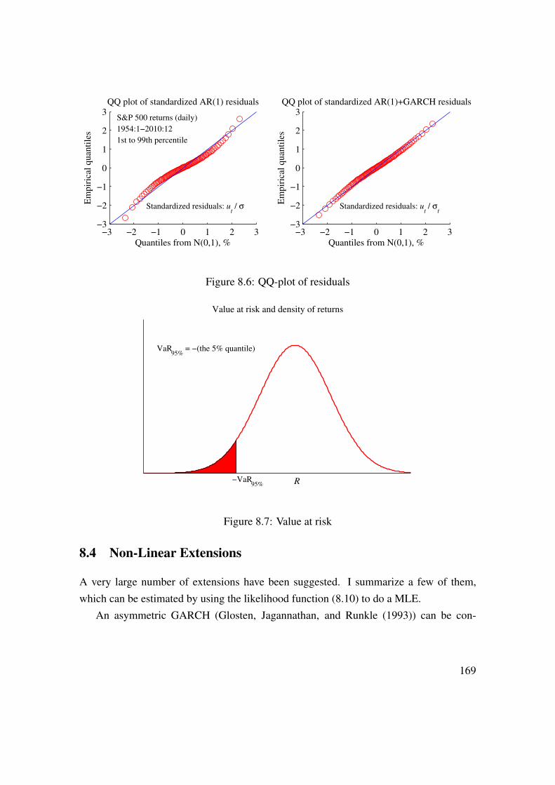
−3 −2 −1 0 1 2 3−3
−2
−1
0
1
2
3
Quantiles from N(0,1), %
Em
pir
ical
quan
tile
s
QQ plot of standardized AR(1) residuals
S&P 500 returns (daily)
1954:1−2010:12
1st to 99th percentile
Standardized residuals: ut / σ
−3 −2 −1 0 1 2 3−3
−2
−1
0
1
2
3
Quantiles from N(0,1), %
Em
pir
ical
quan
tile
s
QQ plot of standardized AR(1)+GARCH residuals
Standardized residuals: ut / σ
t
Figure 8.6: QQ-plot of residuals
Value at risk and density of returns
R−VaR95%
VaR95%
= −(the 5% quantile)
Figure 8.7: Value at risk
8.4 Non-Linear Extensions
A very large number of extensions have been suggested. I summarize a few of them,which can be estimated by using the likelihood function (8.10) to do a MLE.
An asymmetric GARCH (Glosten, Jagannathan, and Runkle (1993)) can be con-
169

1980 1990 2000 20100
1
2
3
4
5GARCH std, %
S&P 500, daily data 1954:1−2010:12
1980 1990 2000 20100
5
10
Value at Risk95%
(one day), %
−4 −2 0 2 40
0.1
0.2
0.3
0.4
Distribution of returns, VaR
Estimated N(), unconditional
Figure 8.8: Conditional volatility and VaR
structed as
�2t D ! C ˛u2t�1 C ˇ�2t�1 C ı.ut�1 > 0/u2t�1, where ı.q/ D(1 if q is true0 else.
(8.14)
This means that the effect of the shock u2t�1 is ˛ if the shock was negative and ˛ C ifthe shock was positive. With < 0, volatility increases more in response to a negativeut�1 (“bad news”) than to a positive ut�1.
The EGARCH (exponential GARCH, Nelson (1991)) sets
ln �2t D ! C ˛jut�1j�t�1
C ˇ ln �2t�1 C ut�1
�t�1(8.15)
Apart from being written in terms of the log (which is a smart trick to make �2t > 0 holdwithout any restrictions on the parameters), this is an asymmetric model. The jut�1j termis symmetric: both negative and positive values of ut�1 affect the volatility in the same
170

way. The linear term in ut�1 modifies this to make the effect asymmetric. In particular,if < 0, then the volatility increases more in response to a negative ut�1 (“bad news”)than to a positive ut�1.
Hentschel (1995) estimates several models of this type, as well as a very generalformulation on daily stock index data for 1926 to 1990 (some 17,000 observations). Moststandard models are rejected in favour of a model where �t depends on �t�1 and jut�1 �bj3=2.
8.5 (G)ARCH-M
It can make sense to let the conditional volatility enter the mean equation—for instance,as a proxy for risk which may influence the expected return.
We modify the “mean equation” (8.4) to include the conditional variance �2t (takenfrom any of the models for heteroskedasticity) as a regressor
yt D x0tb C '�2t C ut : (8.16)
Note that �2t is predetermined, since it is a function of information in t � 1. This modelcan be estimated by using the likelihood function (8.10) to do MLE.
Remark 8.6 (Coding of (G)ARCH-M) We can use the same approach as in Remark 8.1,
except that we use (8.16) instead of (8.4) to calculate the residuals (and that we obviously
also need a guess of ').
Example 8.7 (Theoretical motivation of GARCH-M) A mean variance investor solves
max˛ ERp � �2pk=2; subject to
Rp D ˛Rm C .1 � ˛/Rf ;
where Rm is the return on the risky asset (the market index) and Rf is the riskfree return.
The solution is
˛ D 1
k
E.Rm �Rf /�2m
:
In equilibrium, this weight is one (since the net supply of bonds is zero), so we get
E.Rm �Rf / D k�2m;
171

which says that the expected excess return is increasing in both the market volatility and
risk aversion (k).
8.6 Multivariate (G)ARCH
8.6.1 Different Multivariate Models
This section gives a brief summary of some multivariate models of heteroskedasticity.Suppose ut is an n � 1 vector. For instance, ut could be the residuals from n differentregressions or just n different demeaned return series.
We define the conditional (on the information set in t � 1) covariance matrix of ut as
˙t D Et�1 utu0t : (8.17)
Remark 8.8 (The vech operator) vech(A) of a matrix A gives a vector with the elements
on and below the principal diagonal A stacked on top of each other (column wise). For
instance, vech
"a11 a12
a21 a22
#D
264 a11
a21
a22
375.
It may seem as if a multivariate (matrix) version of the GARCH(1,1) model wouldbe simple, but it is not. The reason is that it would contain far too many parameters.Although we only need to care about the unique elements of ˙t , that is, vech.˙t/, thisstill gives very many parameters
vech.˙t/ D C C Avech.ut�1u0t�1/C Bvech.˙t�1/: (8.18)
For instance, with n D 2 we have264 �11;t
�21;t
�22;t
375 D C C A264 u21;t�1
u1;t�1u2;t�1
u22;t�1
375C B264 �11;t�1
�21;t�1
�22;t�1
375 ; (8.19)
where C is 3 � 1, A is 3 � 3, and B is 3 � 3. This gives 21 parameters, which is alreadyhard to manage. We have to limit the number of parameters. We also have to find away to impose restrictions so ˙t is positive definite (compare the restrictions of positivecoefficients in (8.12)).
172

The Diagonal Model
The diagonal model assumes that A and B are diagonal. This means that every elementof ˙t follows a univariate process. With n D 2 we have264 �11;t
�21;t
�22;t
375 D264c1c2c3
375C264a1 0 0
0 a2 0
0 0 a3
375264 u21;t�1
u1;t�1u2;t�1
u22;t�1
375C264b1 0 0
0 b2 0
0 0 b3
375264 �11;t�1
�21;t�1
�22;t�1
375 ;(8.20)
which gives 3C 3C 3 D 9 parameters (in C , A, and B , respectively). To make sure that˙t is positive definite we have to impose further restrictions. The obvious drawback ofthis model is that there is no spillover of volatility from one variable to another.
The Constant Correlation Model
The constant correlation model assumes that every variance follows a univariate GARCHprocess and that the conditional correlations are constant. With n D 2 the covariancematrix is"
�11;t �12;t
�12;t �22;t
#D"p
�11;t 0
0p�22;t
#"1 �12
�12 1
#"p�11;t 0
0p�22;t
#(8.21)
and each of �11t and �22t follows a GARCH process. Assuming a GARCH(1,1) as in(8.12) gives 7 parameters (2 � 3 GARCH parameters and one correlation), which is con-venient. The price is, of course, the assumption of no movements in the correlations. Toget a positive definite ˙t , each individual GARCH model must generate a positive vari-ance (same restrictions as before), and that all the estimated (constant) correlations arebetween �1 and 1.
Remark 8.9 (Estimating the constant correlation model) A quick (and dirty) method for
estimating is to first estimate the individual GARCH processes and then estimate the cor-
relation of the standardized residuals u1t=p�11;t and u2t=
p�22;t .
By also specifying how the correlation can change over time, we get a dynamic cor-
relation model. It is slightly harder to estimate.See Figure 8.9 for an illustration.
173
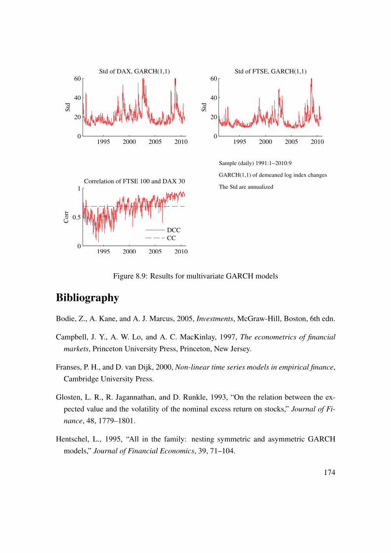
1995 2000 2005 20100
20
40
60Std of DAX, GARCH(1,1)
Std
1995 2000 2005 20100
20
40
60Std of FTSE, GARCH(1,1)
Std
1995 2000 2005 20100
0.5
1Correlation of FTSE 100 and DAX 30
Corr
DCC
CC
Sample (daily) 1991:1−2010:9
GARCH(1,1) of demeaned log index changes
The Std are annualized
Figure 8.9: Results for multivariate GARCH models
Bibliography
Bodie, Z., A. Kane, and A. J. Marcus, 2005, Investments, McGraw-Hill, Boston, 6th edn.
Campbell, J. Y., A. W. Lo, and A. C. MacKinlay, 1997, The econometrics of financial
markets, Princeton University Press, Princeton, New Jersey.
Franses, P. H., and D. van Dijk, 2000, Non-linear time series models in empirical finance,Cambridge University Press.
Glosten, L. R., R. Jagannathan, and D. Runkle, 1993, “On the relation between the ex-pected value and the volatility of the nominal excess return on stocks,” Journal of Fi-
nance, 48, 1779–1801.
Hentschel, L., 1995, “All in the family: nesting symmetric and asymmetric GARCHmodels,” Journal of Financial Economics, 39, 71–104.
174

Nelson, D. B., 1991, “Conditional heteroskedasticity in asset returns,” Econometrica, 59,347–370.
Taylor, S. J., 2005, Asset price dynamics, volatility, and prediction, Princeton UniversityPress.
Verbeek, M., 2004, A guide to modern econometrics, Wiley, Chichester, 2nd edn.
175

.D..3
9 Risk Measures
Reference: Hull (2006) 18; McDonald (2006) 25; Fabozzi, Focardi, and Kolm (2006)4–5; McNeil, Frey, and Embrechts (2005)
9.1 Symmetric Dispersion Measures
9.1.1 Mean Absolute Deviation
The variance (and standard deviation) is very sensitive to the tails of the distribution.For instance, even if the standard normal distribution and a student-t distribution with4 degrees of freedom look fairly similar, the latter has a variance that is twice as large(recall: the variance of a tn distribution is n=.n � 2/ for n > 2). This may or may not bewhat the investor cares about. If not, the mean absolute deviation is an alternative. Let �be the mean, then the definition is
mean absolute deviation D E jR � �j: (9.1)
This measure of dispersion is much less sensitive to the tails—essentially because it doesnot involve squaring the variable.
Notice, however, that for a normally distributed return the mean absolute deviationis proportional to the standard deviation—see Remark 9.1. Both measures will thereforelead to the same portfolio choice (for a given mean return). In other cases, the portfoliochoice will be different (and perhaps complicated to perform since it is typically not easyto calculate the mean absolute deviation of a portfolio).
Remark 9.1 (Mean absolute deviation of N.�; �2/ and tn) If R � N.�; �2/, then
E jR � �j Dp2=�� � 0:8�:
If R � tn, then E jRj D 2pn=Œ.n � 1/B.n=2; 0:5/�, where B is the beta function. For
n D 4, E jRj D 1 which is just 25% higher than for a N.0; 1/ distribution. In contrast,
176

the standard deviation isp2, which is 41% higher than for the N.0; 1/.
See Table 9.1 for an empirical illustration.
Small growth Large valueStd 8.4 5.0VaR (95%) 12.4 7.5ES (95%) 17.3 10.3SemiStd 5.5 3.2Drawdown 77.9 49.4
Table 9.1: Risk measures of monthly returns of two stock indices (%), US data 1957:1-2009:12.
9.1.2 Index Tracking Errors
Value at risk and density of returns
R−VaR95%
VaR95%
= −(the 5% quantile)
Figure 9.1: Value at risk
Suppose instead that our task, as fund managers, say, is to track a benchmark portfolio(returns Rb and portfolio weights wb)—but we are allowed to make some deviations. Forinstance, we are perhaps asked to track a certain index. The deviations, typically measuredin terms of the variance of the tracking errors for the returns, can be motivated by practical
177

considerations and by concerns about trading costs. If our portfolio has the weights w,then the portfolio return is Rp D w0R, where R are the original assets. Similarly, thebenchmark portfolio (index) has the return Rb D w0
bR. If the variance of the tracking
error should be less than U , then we have the restriction
Var.Rp �Rb/ D .w � wb/0˙.w � wb/ � U; (9.2)
where ˙ is the covariance matrix of the original assets. This type of restriction is fairlyeasy to implement numerically in the portfolio choice model (the optimization problem).
9.2 Downside Risk
9.2.1 Value at Risk
The mean-variance framework is often criticized for failing to distinguish between down-side (considered to be risk) and upside (considered to be potential).
The 95% Value at Risk (VaR95%) says that there is only a 5% chance that the return(R) will be less than �VaR95%
Pr.R � �VaR˛/ D 1 � ˛: (9.3)
See Figure 9.1.
Example 9.2 (Quantile of a distribution) The 0.05 quantile is the value such that there is
only a 5% probability of a lower number, Pr.R �quantile0:05/ D 0:05.
We can solve this expression for the VaR˛ as
VaR˛ D � cdf�1R .1 � ˛/, (9.4)
where cdf�1R ./ is the inverse cumulative distribution function of the returns, so cdf�1R .1 �˛/ is the 1 � ˛ quantile (or “critical value”) of the return distribution. For instance,VaR95% is the negative of the 0:05 quantile of the return distribution. Notice that the returndistribution depends on the investment horizon, so a value at risk measure is typicallycalculated for a stated investment period (for instance, one day).
178

If the return is normally distributed, R � N.�; �2/ and c1�˛ is the 1 � ˛ quantile ofa N(0,1) distribution (for instance, �1:64 for 1 � ˛ D 1 � 0:95), then
VaR˛ D �.�C c1�˛�/: (9.5)
This is illustrated in Figure 9.2.Notice that the value at risk for a normally distributed return is a strictly increasing
function of the standard deviation (and the variance). Minimizing the VaR at a given meanreturn therefore gives the same solution (portfolio weights) as minimizing the variance atthe same given mean return. In other cases, the portfolio choice will be different (andperhaps complicated to perform).
Remark 9.3 (Critical values of N.�; �2/) If R � N.�; �2/, then there is a 5% proba-
bility that R � �� 1:64� , a 2.5% probability that R � �� 1:96� , and a 1% probability
that R � � � 2:33� .
Example 9.4 (VaR with R � N.�; �2/) If daily returns have � D 8% and � D 16%,
then the 1-day VaR95% D �.0:08�1:64�0:16/ � 0:18; we are 95% sure that we will not
loose more than 18% of the investment over one day, that is, VaR95% D 0:18. Similarly,
VaR97:5% D �.0:08 � 1:96 � 0:16/ � 0:24.
Example 9.5 (VaR and regulation of bank capital) Bank regulations have used 3 times
the 99% VaR for 10-day returns as the required bank capital.
Remark 9.6 (Multi-period VaR) If the returns are iid, then a q-period return has the
mean q� and variance q�2, where � and �2 are the mean and variance of the one-period
returns respectively. If the mean is zero, then the q-day VaR ispq times the one-day VaR.
Remark 9.7 (VaR from t-distribution) The assumption of normally distributed returns
rules thick tails. As an alternative, suppose the normalized return has a t-distribution
with v degrees of freedomR � �s� tv:
Notice that s2 is not the variance of R, since Var.R/ D vs2=.v � 2/ (assuming v > 2,
so the variance is defined). In this case, (9.5) still holds, but with c1�˛ calculated as
179

−3 0 30
0.1
0.2
0.3
0.4
Density of N(0,1)
c
5% quantile is c = −1.64
x
−40 0 400
1
2
3Density of N(8,16
2)
R
5% quantile is µ + c*σ = −18
−40 0 400
0.5
1
cdf of N(8,162)
R
cdf
0 0.2 0.4 0.6 0.8 1
−40
0
40
Inverse of cdf of N(8,162)
cdf
R
Figure 9.2: Finding critical value of N(�,�2) distribution
the 1 � ˛ quantile of a tv distribution. In practice, for a given value of Var.R/, the t
distribution gives a smaller value of the VaR than the normal distribution. The reason is
that the variance of a t-distribution is very high for low degrees of freedom.
The VaR concept has been criticized for having poor aggregation properties. In par-ticular, the VaR for a portfolio is not necessarily (weakly) lower than the portfolio of theVaRs, which contradicts the notion of diversification benefits. (To get this unfortunateproperty, the return distributions must be heavily skewed.)
Figures 9.3–9.4 illustrate the VaR calculated from a time series model (to be precise,a AR(1)+GARCH(1,1) model) for daily S&P returns.
Remark 9.8 (Backtesting VaR) Figure 9.3 shows the results from “backtesting” a VaR
model (in particular model the volatility is time-varying according to a GARCH model).
For instance, we first find the VaR95% and then calculate what fraction of returns that is
180

1980 1990 2000 20100
1
2
3
4
5GARCH std, %
S&P 500, daily data 1954:1−2010:12
1980 1990 2000 20100
5
10
Value at Risk95%
(one day), %
−4 −2 0 2 40
0.1
0.2
0.3
0.4
Distribution of returns, VaR
Estimated N(), unconditional
Figure 9.3: Conditional volatility and VaR
actually below this number. If the model is correct it should be 5%. We then repeat this
for VaR96% (only 4% of the returns should be below this number).
9.2.2 Expected Shortfall
The expected shortfall (also called conditional VaR) is the expected loss when the returnactually is below the VaR˛, that is,
ES˛ D �E.RjR � �VaR˛/: (9.6)
This might be more informative than the VaR˛, which is the minimum loss that will happenwith a 1 � ˛ probability.
181

0 0.02 0.04 0.06 0.08 0.10
0.01
0.02
0.03
0.04
0.05
0.06
0.07
0.08
0.09
0.1
Theoretical Prob(R<VaR)
Em
pir
ical
Pro
b(R
<V
aR)
Backtesting VaR from GARCH(1,1), daily S&P 500 returns
Daily S&P 500 returns, 1954:1−2010:12
Figure 9.4: Backtesting VaR from a GARCH model, assuming normally distributedshocks
For a normally distributed return R � N.�; �2/ we have
ES˛ D ��C � �.c1�˛/1 � ˛ ; (9.7)
where �./ is the pdf or aN.0; 1/ variable and where c1�˛ is the 1�˛ quantile of a N(0,1)distribution (for instance, �1:64 for 1 � ˛ D 0:05).
Proof. (of (9.7)) If x � N.�; �2/, then E.xjx � b/ D � � ��.b0/=˚.b0/ whereb0 D .b � �/=� and where �./ and ˚./ are the pdf and cdf of a N.0; 1/ variablerespectively. To apply this, use b D �VaR˛ so b0 D c1�˛. Clearly, ˚.c1�˛/ D 1� ˛ (bydefinition of the 1 � ˛ quantile). Multiply by �1.
Example 9.9 (ES) If � D 8% and � D 16%, the 95% expected shortfall is ES95% D�0:08 C 0:16�.�1:64/=0:05 � 0:25 and the 97.5% expected shortfall is ES97:5% D�0:08C 0:16�.�1:96/=0:025 � 0:29.
Notice that the expected shortfall for a normally distributed return (9.7) is a strictly
182
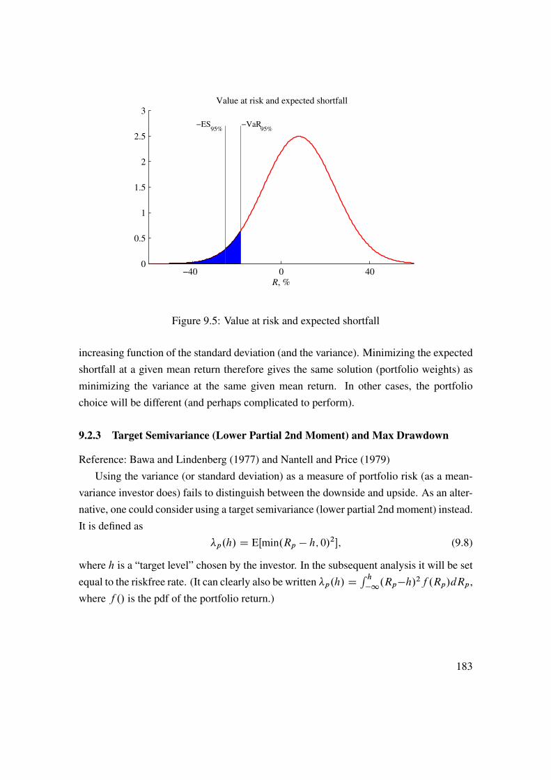
−40 0 400
0.5
1
1.5
2
2.5
3Value at risk and expected shortfall
R, %
−ES95%
−VaR95%
Figure 9.5: Value at risk and expected shortfall
increasing function of the standard deviation (and the variance). Minimizing the expectedshortfall at a given mean return therefore gives the same solution (portfolio weights) asminimizing the variance at the same given mean return. In other cases, the portfoliochoice will be different (and perhaps complicated to perform).
9.2.3 Target Semivariance (Lower Partial 2nd Moment) and Max Drawdown
Reference: Bawa and Lindenberg (1977) and Nantell and Price (1979)Using the variance (or standard deviation) as a measure of portfolio risk (as a mean-
variance investor does) fails to distinguish between the downside and upside. As an alter-native, one could consider using a target semivariance (lower partial 2nd moment) instead.It is defined as
�p.h/ D EŒmin.Rp � h; 0/2�; (9.8)
where h is a “target level” chosen by the investor. In the subsequent analysis it will be setequal to the riskfree rate. (It can clearly also be written �p.h/ D
R h�1.Rp�h/2f .Rp/dRp,
where f ./ is the pdf of the portfolio return.)
183

−60 −40 −20 0 20 40 600
1
2
3Probability density function (pdf)
N(µ,σ2)
µ = 0.08
σ = 0.16
x, %
−60 −40 −20 0 20 40 600
0.02
0.04
Contribution to variance
pdf(x)(x−µ)2
Var(x)=area
x, %
−60 −40 −20 0 20 40 600
0.02
0.04
Contribution to target semivariance
pdf(x)min(x−0.02,0)2
target semivariance(x)=area
x, %
0 0.02 0.04 0.060
0.005
0.01
0.015
0.02
Target semivariance as function of σ2
σ2
N(0.08,σ2)
Target level: 0.02
Figure 9.6: Target semivariance as a function of mean and standard deviation for aN(�,�2) variable
In comparison with a variance
�2p D E.Rp � �p/2; (9.9)
the target semivariance differs on two accounts: (i) it uses the target level h as a referencepoint instead of the mean �p: and (ii) only negative deviations from the reference pointare given any weight. See Figure 9.6 for an illustration (based on a normally distributedvariable).
For a normally distributed variable, the target semivariance �p.h/ is increasing in thestandard deviation (for a given mean)—see Remark 9.10. See also Figure 9.6 for anillustration. This means that minimizing �p.h/ at a given mean return gives the samesolution (portfolio weights) as minimizing �p (or �2p ) at the same given mean return. As
184

0 5 10 150
5
10
15Std and mean
Std, %
Mea
n, %
The markers for target semivariance (sv) indicate the stdof the portfolio that minimizes the target semivariance at the given mean return
MV (risky)
MV (risky&riskfree)
target sv (risky)
target sv (risky&riskfree)
Figure 9.7: Standard deviation and expected returns
time
pric
e
max
draw
dow
n
Figure 9.8: Max drawdown
a result, with normally distributed returns, an investor who wants to minimize the lowerpartial 2nd moment (at a given mean return) is behaving just like a mean-variance investor.In other cases, the portfolio choice will be different (and perhaps complicated to perform).
See Figure 9.7 for an illustration.An alternative measure is the (percentage) maximum drawdown over a given horizon,
for instance, 5 years, say. This is the largest loss from peak to bottom within the givenhorizon–see Figure 9.8. This is a useful measure when the investor do not know exactlywhen he/she has to exit the investment—since it indicates the worst (peak to bottom)outcome over the sample.
185
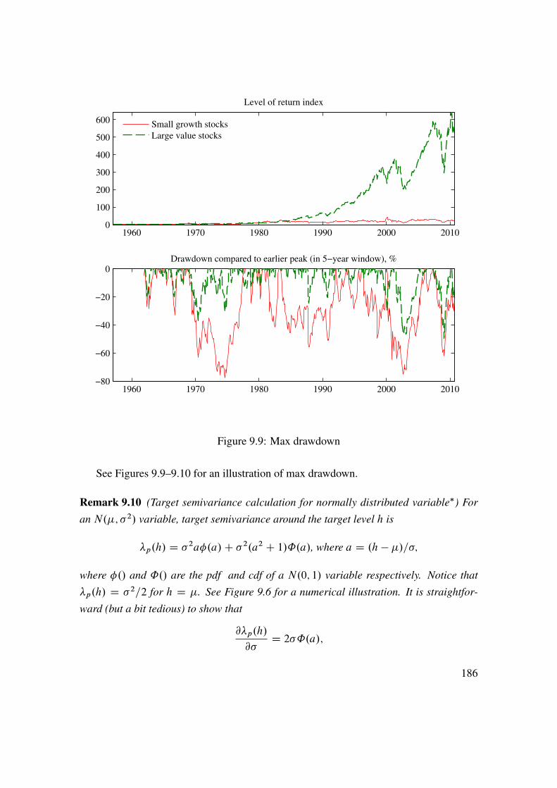
1960 1970 1980 1990 2000 20100
100
200
300
400
500
600
Level of return index
Small growth stocks
Large value stocks
1960 1970 1980 1990 2000 2010−80
−60
−40
−20
0Drawdown compared to earlier peak (in 5−year window), %
Figure 9.9: Max drawdown
See Figures 9.9–9.10 for an illustration of max drawdown.
Remark 9.10 (Target semivariance calculation for normally distributed variable�) For
an N.�; �2/ variable, target semivariance around the target level h is
�p.h/ D �2a�.a/C �2.a2 C 1/˚.a/, where a D .h � �/=�;
where �./ and ˚./ are the pdf and cdf of a N.0; 1/ variable respectively. Notice that
�p.h/ D �2=2 for h D �. See Figure 9.6 for a numerical illustration. It is straightfor-
ward (but a bit tedious) to show that
@�p.h/
@�D 2�˚.a/;
186

1995 1997 2000 2002 2005 2007 20100
1
2
3
4
Level of return index
MSCI world
CT hedge funds
Global govt bonds
1995 1997 2000 2002 2005 2007 2010−60
−50
−40
−30
−20
−10
0Drawdown compared to earlier peak (since start of sample), %
Figure 9.10: Max drawdown
so the target semivariance is a strictly increasing function of the standard deviation.
See Table 9.2 for an empirical comparison of the different risk measures.
Std VaR (95%) ES (95%) SemiStd DrawdownStd 1.00 0.96 0.97 0.96 0.67VaR (95%) 0.96 1.00 0.98 0.99 0.64ES (95%) 0.97 0.98 1.00 0.99 0.64SemiStd 0.96 0.99 0.99 1.00 0.66Drawdown 0.67 0.64 0.64 0.66 1.00
Table 9.2: Correlation of risk measures across monthly returns of the 25 FF portfolios(%), US data 1957:1-2009:12.
187

−20 −10 0 100
2000
4000
6000
8000
Daily excess return, %
Num
ber
of
day
s
Daily returns, full
−20 −10 0 100
5
10
15
20
25
Daily excess return, %
Num
ber
of
day
s
Daily returns, zoomed in vertically
−3 −2 −1 0 1 2 30
2000
4000
6000
8000
Daily excess return, %
Num
ber
of
day
s
Daily returns, zoomed in horizontally
Daily S&P 500 returns, 1957:1−2010:9
The solid line is an estimated normal distribution
Figure 9.11: Distribution of daily S&P returns
9.3 Empirical Return Distributions
Are returns normally distributed? Mostly not, but it depends on the asset type and on thedata frequency. Options returns typically have very non-normal distributions (in partic-ular, since the return is �100% on many expiration days). Stock returns are typicallydistinctly non-linear at short horizons, but can look somewhat normal at longer horizons.
To assess the normality of returns, the usual econometric techniques (Bera–Jarqueand Kolmogorov-Smirnov tests) are useful, but a visual inspection of the histogram and aQQ-plot also give useful clues. See Figures 9.11–9.13 for illustrations.
Remark 9.11 (Reading a QQ plot) A QQ plot is a way to assess if the empirical distri-
bution conforms reasonably well to a prespecified theoretical distribution, for instance,
a normal distribution where the mean and variance have been estimated from the data.
Each point in the QQ plot shows a specific percentile (quantile) according to the empiri-
188

−6 −4 −2 0 2 4 6
−6
−4
−2
0
2
4
6
Quantiles from estimated N(µ,σ2), %
Em
pir
ical
quan
tile
s
QQ plot of daily S&P 500 returns
Daily S&P 500 returns, 1957:1−2010:9
0.1th to 99.9th percentiles
Figure 9.12: Quantiles of daily S&P returns
cal as well as according to the theoretical distribution. For instance, if the 2th percentile
(0.02 percentile) is at -10 in the empirical distribution, but at only -3 in the theoretical
distribution, then this indicates that the two distributions have fairly different left tails.
There is one caveat to this way of studying data: it only provides evidence on theunconditional distribution. For instance, nothing rules out the possibility that we couldestimate a model for time-varying volatility (for instance, a GARCH model) of the returnsand thus generate a description for how the VaR changes over time. However, data withtime varying volatility will typically not have an unconditional normal distribution.
Bibliography
Bawa, V. S., and E. B. Lindenberg, 1977, “Capital market equilibrium in a mean-lowerpartial moment framework,” Journal of Financial Economics, 5, 189–200.
189

−6 −4 −2 0 2 4 6
−5
0
5
Quantiles from N(µ,σ2), %
Em
pir
ical
quan
tile
sQQ plot of daily returns
−10 −5 0 5 10
−10
−5
0
5
10
Quantiles from N(µ,σ2), %
Em
pir
ical
quan
tile
s
QQ plot of weekly returns
−20 −10 0 10
−20
−10
0
10
Quantiles from N(µ,σ2), %
Em
pir
ical
quan
tile
s
QQ plot of monthly returns Circles denote 0.1th to 99.9th percentiles
Daily S&P 500 returns, 1957:1−2010:9
Figure 9.13: Distribution of S&P returns (different horizons)
Fabozzi, F. J., S. M. Focardi, and P. N. Kolm, 2006, Financial modeling of the equity
market, Wiley Finance.
Hull, J. C., 2006, Options, futures, and other derivatives, Prentice-Hall, Upper SaddleRiver, NJ, 6th edn.
McDonald, R. L., 2006, Derivatives markets, Addison-Wesley, 2nd edn.
McNeil, A. J., R. Frey, and P. Embrechts, 2005, Quantitative risk management, PrincetonUniversity Press.
Nantell, T. J., and B. Price, 1979, “An analytical comparison of variance and semivariancecapital market theories,” Journal of Financial and Quantitative Analysis, 14, 221–242.
190

10 Return Distributions (Univariate)
Sections denoted by a star (�) is not required reading.
10.1 Estimating and Testing Distributions
Reference: Harvey (1989) 260, Davidson and MacKinnon (1993) 267, Silverman (1986);Mittelhammer (1996), DeGroot (1986)
10.1.1 A Quick Recap of a Univariate Distribution
The cdf (cumulative distribution function) measures the probability that the random vari-able Xi is below or at some numerical value xi ,
ui D Fi.xi/ D Pr.Xi � xi/: (10.1)
For instance, with an N.0; 1/ distribution, F.�1:64/ D 0:05. Clearly, the cdf valuesare between (and including) 0 and 1. The distribution of Xi is often called the marginal
distribution of Xi—to distinguish it from the joint distribution of Xi and Xj . (See belowfor more information on joint distributions.)
The pdf (probability density function) fi.xi/ is the “height” of the distribution in thesense that the cdf F.xi/ is the integral of the pdf from minus infinity to xi
Fi.xi/ DZ xi
sD�1
fi.s/ds: (10.2)
(Conversely, the pdf is the derivative of the cdf, fi.xi/ D @Fi.xi/=@xi .) The Gaussianpdf (the normal distribution) is bell shaped.
Remark 10.1 (Quantile of a distribution) The ˛ quantile of a distribution (�˛) is the value
of x such that there is a probability of ˛ of a lower value. We can solve for the quantile by
inverting the cdf, ˛ D F.�˛/ as �˛ D F �1.˛/. For instance, the 5% quantile of a N.0; 1/
distribution is �1:64 D ˚�1.0:05/, where ˚�1./ denotes the inverse of an N.0; 1/ cdf.
See Figure 10.1 for an illustration.
191

−3 0 30
0.1
0.2
0.3
0.4
Density of N(0,1)
c
5% quantile is c = −1.64
x
−40 0 400
1
2
3Density of N(8,16
2)
R
5% quantile is µ + c*σ = −18
−40 0 400
0.5
1
cdf of N(8,162)
R
cdf
0 0.2 0.4 0.6 0.8 1
−40
0
40
Inverse of cdf of N(8,162)
cdf
R
Figure 10.1: Finding quantiles of a N(�,�2) distribution
10.1.2 QQ Plots
Are returns normally distributed? Mostly not, but it depends on the asset type and on thedata frequency. Options returns typically have very non-normal distributions (in partic-ular, since the return is �100% on many expiration days). Stock returns are typicallydistinctly non-linear at short horizons, but can look somewhat normal at longer horizons.
To assess the normality of returns, the usual econometric techniques (Bera–Jarqueand Kolmogorov-Smirnov tests) are useful, but a visual inspection of the histogram and aQQ-plot also give useful clues. See Figures 10.2–10.4 for illustrations.
Remark 10.2 (Reading a QQ plot) A QQ plot is a way to assess if the empirical distri-
bution conforms reasonably well to a prespecified theoretical distribution, for instance,
a normal distribution where the mean and variance have been estimated from the data.
Each point in the QQ plot shows a specific percentile (quantile) according to the empiri-
192

cal as well as according to the theoretical distribution. For instance, if the 2th percentile
(0.02 percentile) is at -10 in the empirical distribution, but at only -3 in the theoretical
distribution, then this indicates that the two distributions have fairly different left tails.
There is one caveat to this way of studying data: it only provides evidence on theunconditional distribution. For instance, nothing rules out the possibility that we couldestimate a model for time-varying volatility (for instance, a GARCH model) of the returnsand thus generate a description for how the VaR changes over time. However, data withtime varying volatility will typically not have an unconditional normal distribution.
−20 −10 0 100
2000
4000
6000
8000
Daily excess return, %
Num
ber
of
day
s
Daily returns, full
−20 −10 0 100
5
10
15
20
25
Daily excess return, %
Num
ber
of
day
s
Daily returns, zoomed in vertically
−3 −2 −1 0 1 2 30
2000
4000
6000
8000
Daily excess return, %
Num
ber
of
day
s
Daily returns, zoomed in horizontally
Daily S&P 500 returns, 1957:1−2010:9
The solid line is an estimated normal distribution
Figure 10.2: Distribution of daily S&P returns
193

−6 −4 −2 0 2 4 6
−6
−4
−2
0
2
4
6
Quantiles from estimated N(µ,σ2), %
Em
pir
ical
quan
tile
s
QQ plot of daily S&P 500 returns
Daily S&P 500 returns, 1957:1−2010:9
0.1th to 99.9th percentiles
Figure 10.3: Quantiles of daily S&P returns
10.1.3 Parametric Tests of Normal Distribution
The skewness, kurtosis and Bera-Jarque test for normality are useful diagnostic tools.They are
Test statistic Distributionskewness D 1
T
PTtD1
�xt��
�
�3N .0; 6=T /
kurtosis D 1T
PTtD1
�xt��
�
�4N .3; 24=T /
Bera-Jarque D T6
skewness2 C T24.kurtosis � 3/2 �22:
(10.3)
This is implemented by using the estimated mean and standard deviation. The distribu-tions stated on the right hand side of (10.3) are under the null hypothesis that xt is iidN��; �2
�. The “excess kurtosis” is defined as the kurtosis minus 3.
The intuition for the �22 distribution of the Bera-Jarque test is that both the skewnessand kurtosis are, if properly scaled, N.0; 1/ variables. It can also be shown that they,under the null hypothesis, are uncorrelated. The Bera-Jarque test statistic is therefore a
194

−6 −4 −2 0 2 4 6
−5
0
5
Quantiles from N(µ,σ2), %
Em
pir
ical
quan
tile
sQQ plot of daily returns
−10 −5 0 5 10
−10
−5
0
5
10
Quantiles from N(µ,σ2), %
Em
pir
ical
quan
tile
s
QQ plot of weekly returns
−20 −10 0 10
−20
−10
0
10
Quantiles from N(µ,σ2), %
Em
pir
ical
quan
tile
s
QQ plot of monthly returns Circles denote 0.1th to 99.9th percentiles
Daily S&P 500 returns, 1957:1−2010:9
Figure 10.4: Distribution of S&P returns (different horizons)
sum of the square of two uncorrelated N.0; 1/ variables, which has a �22 distribution.
10.1.4 Nonparametric Tests of General Distributions
The Kolmogorov-Smirnov test is designed to test if an empirical distribution function,EDF.x/, conforms with a theoretical cdf, F .x/. The empirical distribution function isdefined as the fraction of observations which are less or equal to x, that is,
EDF .x/ D 1
T
TXtD1
ı.xt � x/; where ı.q/ D(1 if q is true0 else.
(10.4)
The EDF.xt/ and F .xt/ are often plotted against the sorted (in ascending order) samplefxtgTtD1.
See Figure 10.5 for an illustration.
195

3 3.5 4 4.5 5 5.5 6
0
0.2
0.4
0.6
0.8
1
Empirical distribution function and theoretical cdf
x
data
cdf of N(4,1)
EDF
Figure 10.5: Example of empirical distribution function
3 3.5 4 4.5 5 5.5 6
0
0.2
0.4
0.6
0.8
1
Kolmogorov−Smirnov test
x
The K−S test statistic isthe length of the longest arrow
data
cdf of N(4,1)
EDF
Figure 10.6: K-S test
Example 10.3 (EDF) Suppose we have a sample with three data points: Œx1; x2; x3� DŒ5; 3:5; 4�. The empirical distribution function is then as in Figure 10.5.
196

Define the absolute value of the maximum distance
DT D maxxtjEDF .xt/ � F .xt/j : (10.5)
Example 10.4 (Kolmogorov-Smirnov test statistic) Figure 10.5 also shows the cumula-
tive distribution function (cdf) of a normally distributed variable. The test statistic (10.5)
is then the largest difference (in absolute terms) of the EDF and the cdf—among the ob-
served values of xt .
We reject the null hypothesis that EDF.x/ D F .x/ ifpTDt > c, where c is a critical
value which can be calculated from
limT!1
Pr�p
TDT � c�D 1 � 2
1XiD1
.�1/i�1 e�2i2c2 : (10.6)
It can be approximated by replacing1 with a large number (for instance, 100). Forinstance, c D 1:35 provides a 5% critical value. See Figure 10.7. There is a correspondingtest for comparing two empirical cdfs.
Pearson’s �2 test does the same thing as the K-S test but for a discrete distribution.Suppose you have K categories with Ni values in category i . The theoretical distributionpredicts that the fraction pi should be in category i , with
PKiD1 pi D 1. Then
KXiD1
.Ni � Tpi/2Tpi
� �2K�1: (10.7)
There is a corresponding test for comparing two empirical distributions.
10.1.5 Fitting a Mixture Normal Distribution to Data�
Reference: Hastie, Tibshirani, and Friedman (2001) 8.5A normal distribution often fits returns poorly. If we need a distribution, then a mixture
of two normals is typically much better, and still fairly simple.The pdf of this distribution is just a weighted average of two different (bell shaped)
pdfs of normal distributions (also called mixture components)
f .xt I�1; �2; �21 ; �22 ; �/ D .1 � �/�.xt I�1; �21 /C ��.xt I�2; �22 /; (10.8)
197
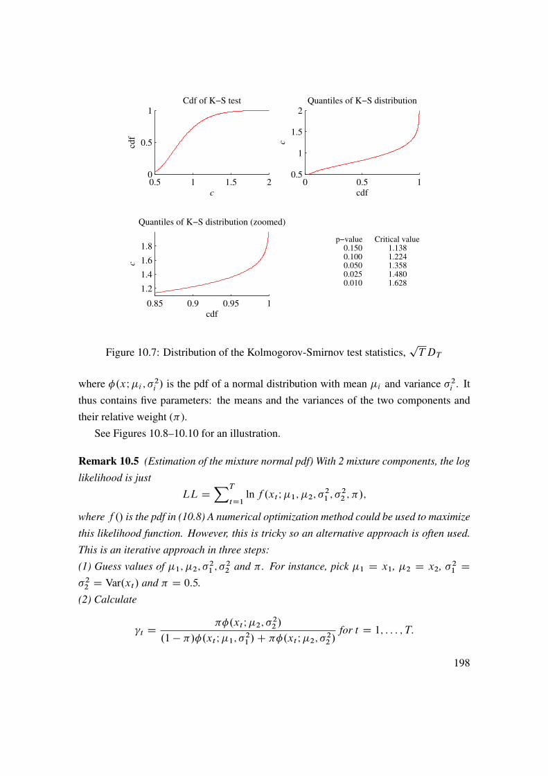
0.5 1 1.5 20
0.5
1Cdf of K−S test
cdf
c
0 0.5 10.5
1
1.5
2Quantiles of K−S distribution
c
cdf
0.85 0.9 0.95 1
1.2
1.4
1.6
1.8
Quantiles of K−S distribution (zoomed)
c
cdf
p−value 0.150 0.100 0.050 0.025 0.010
Critical value 1.138 1.224 1.358 1.480 1.628
Figure 10.7: Distribution of the Kolmogorov-Smirnov test statistics,pTDT
where �.xI�i ; �2i / is the pdf of a normal distribution with mean �i and variance �2i . Itthus contains five parameters: the means and the variances of the two components andtheir relative weight (�).
See Figures 10.8–10.10 for an illustration.
Remark 10.5 (Estimation of the mixture normal pdf) With 2 mixture components, the log
likelihood is just
LL DXT
tD1lnf .xt I�1; �2; �21 ; �22 ; �/;
where f ./ is the pdf in (10.8) A numerical optimization method could be used to maximize
this likelihood function. However, this is tricky so an alternative approach is often used.
This is an iterative approach in three steps:
(1) Guess values of �1; �2; �21 ; �22 and � . For instance, pick �1 D x1, �2 D x2, �21 D
�22 D Var.xt/ and � D 0:5.
(2) Calculate
t D ��.xt I�2; �22 /.1 � �/�.xt I�1; �21 /C ��.xt I�2; �22 /
for t D 1; : : : ; T:
198

−5 −4 −3 −2 −1 0 1 2 3 4 50
0.1
0.2
0.3
0.4
0.5
0.6
Distribution of of S&P500,1957:1−2010:9
Monthly excess return, %
normal pdf
Figure 10.8: Histogram of returns and a fitted normal distribution
(3) Calculate (in this order)
�1 DPT
tD1.1 � t/xtPTtD1.1 � t/
, �21 DPT
tD1.1 � t/.xt � �1/2PTtD1.1 � t/
;
�2 DPT
tD1 txtPTtD1 t
, �22 DPT
tD1 t.xt � �2/2PTtD1 t
, and
� DXT
tD1 t=T .
Iterate over (2) and (3) until the parameter values converge. (This is an example of the
EM algorithm.) Notice that the calculation of �2i uses �i from the same (not the previous)
iteration.
10.1.6 Kernel Density Estimation
Reference: Silverman (1986)A histogram is just a count of the relative number of observations that fall in (pre-
199
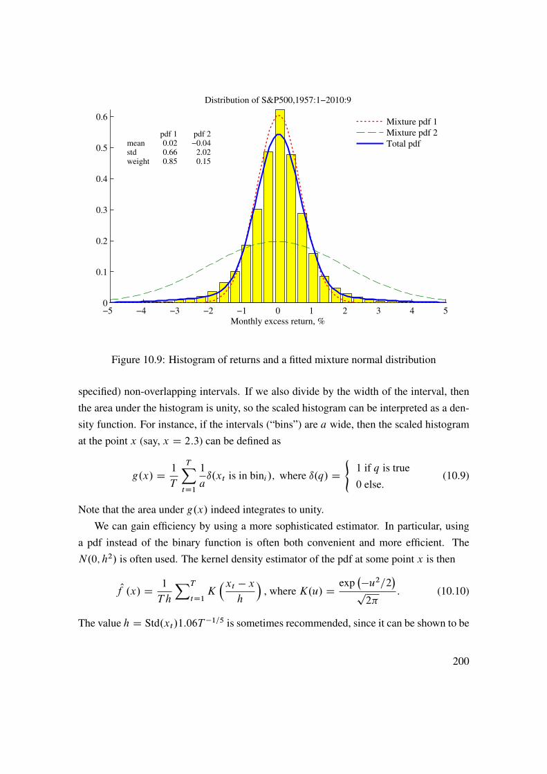
−5 −4 −3 −2 −1 0 1 2 3 4 50
0.1
0.2
0.3
0.4
0.5
0.6
Distribution of S&P500,1957:1−2010:9
Monthly excess return, %
mean std weight
pdf 1 0.02 0.66 0.85
pdf 2 −0.04 2.02 0.15
Mixture pdf 1
Mixture pdf 2
Total pdf
Figure 10.9: Histogram of returns and a fitted mixture normal distribution
specified) non-overlapping intervals. If we also divide by the width of the interval, thenthe area under the histogram is unity, so the scaled histogram can be interpreted as a den-sity function. For instance, if the intervals (“bins”) are a wide, then the scaled histogramat the point x (say, x D 2:3) can be defined as
g.x/ D 1
T
TXtD1
1
aı.xt is in bini/; where ı.q/ D
(1 if q is true0 else.
(10.9)
Note that the area under g.x/ indeed integrates to unity.We can gain efficiency by using a more sophisticated estimator. In particular, using
a pdf instead of the binary function is often both convenient and more efficient. TheN.0; h2/ is often used. The kernel density estimator of the pdf at some point x is then
Of .x/ D 1
T h
XT
tD1K�xt � x
h
�, where K.u/ D exp
��u2=2�p2�
: (10.10)
The value h D Std.xt/1:06T �1=5 is sometimes recommended, since it can be shown to be
200
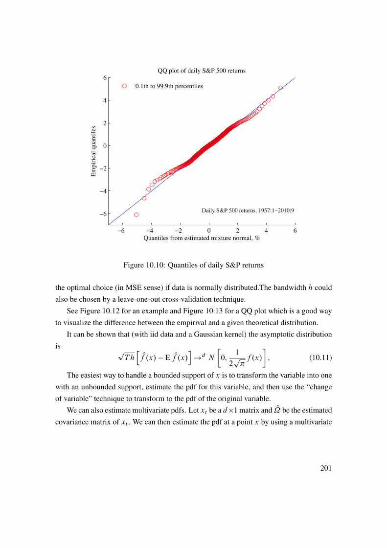
−6 −4 −2 0 2 4 6
−6
−4
−2
0
2
4
6
Quantiles from estimated mixture normal, %
Em
pir
ical
quan
tile
s
QQ plot of daily S&P 500 returns
Daily S&P 500 returns, 1957:1−2010:9
0.1th to 99.9th percentiles
Figure 10.10: Quantiles of daily S&P returns
the optimal choice (in MSE sense) if data is normally distributed.The bandwidth h couldalso be chosen by a leave-one-out cross-validation technique.
See Figure 10.12 for an example and Figure 10.13 for a QQ plot which is a good wayto visualize the difference between the empirival and a given theoretical distribution.
It can be shown that (with iid data and a Gaussian kernel) the asymptotic distributionis p
T hh Of .x/ � E Of .x/
i!d N
�0;
1
2p�f .x/
�; (10.11)
The easiest way to handle a bounded support of x is to transform the variable into onewith an unbounded support, estimate the pdf for this variable, and then use the “changeof variable” technique to transform to the pdf of the original variable.
We can also estimate multivariate pdfs. Let xt be a d�1matrix and O be the estimatedcovariance matrix of xt . We can then estimate the pdf at a point x by using a multivariate
201
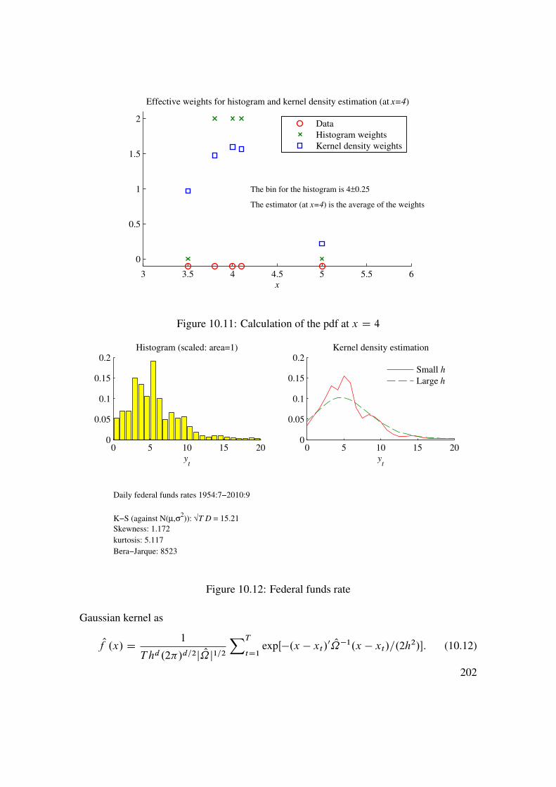
3 3.5 4 4.5 5 5.5 6
0
0.5
1
1.5
2
Effective weights for histogram and kernel density estimation (at x=4)
x
The bin for the histogram is 4±0.25
The estimator (at x=4) is the average of the weights
Data
Histogram weights
Kernel density weights
Figure 10.11: Calculation of the pdf at x D 4
0 5 10 15 200
0.05
0.1
0.15
0.2Histogram (scaled: area=1)
yt
0 5 10 15 200
0.05
0.1
0.15
0.2Kernel density estimation
yt
Small h
Large h
Daily federal funds rates 1954:7−2010:9
K−S (against N(µ,σ2)): √T D = 15.21
Skewness: 1.172
kurtosis: 5.117
Bera−Jarque: 8523
Figure 10.12: Federal funds rate
Gaussian kernel as
Of .x/ D 1
T hd .2�/d=2j O j1=2XT
tD1expŒ�.x � xt/0 O �1.x � xt/=.2h2/�: (10.12)
202

−5 0 5 10 15 20
−5
0
5
10
15
20
Quantiles from estimated N(µ,σ2), %
Em
pir
ical
quan
tile
s
QQ plot of daily federal funds rates
Daily federal funds rates, 1954:7−2010:9
0.1th to 99.9th percentiles
Figure 10.13: Federal funds rate
The value h D 0:96T �1=.dC4/ is sometimes recommended.
10.1.7 “Foundations of Technical Analysis...” by Lo, Mamaysky and Wang (2000)
Reference: Lo, Mamaysky, and Wang (2000)Topic: is the distribution of the return different after a “signal” (TA). This paper uses
kernel regressions to identify and implement some technical trading rules, and then testsif the distribution (of the return) after a signal is the same as the unconditional distribution(using Pearson’s �2 test and the Kolmogorov-Smirnov test). They reject that hypothesisin many cases, using daily data (1962-1996) for around 50 (randomly selected) stocks.
See Figures 10.14–10.15 for an illustration.
10.2 Tail Distribution
Reference: McNeil, Frey, and Embrechts (2005) 7, Alexander (2008) 3
203

Jan Feb Mar Apr1150
1200
1250
1300
1350
1999
Inverted MA rule, S&P 500
MA(3) and MA(25), bandwidth 0.01
Long MA (−)
Long MA (+)
Short MA
Figure 10.14: Examples of trading rules
In risk control, the focus is the distribution of losses beyond some threshold level.This has three direct implications. First, the object under study is the loss
X D �R; (10.13)
that is, the negative of the return. Second, the attention is on how the distribution lookslike beyond a threshold and also on the the probability of exceeding this threshold. In con-trast, the exact shape of the distribution below that point is typically disregarded. Third,modelling the tail of the distribution is best done by using a distribution that allows for amuch heavier tail that suggested by a normal distribution. The generalized Pareto (GP)distribution is often used.
10.2.1 Loss Distribution and the Generalized Pareto Distribution
The generalized Pareto (GP) distribution is often used to model the tail of the loss distri-bution. See Figure 10.16 for an illustration.
Remark 10.6 (Cdf and pdf of the generalized Pareto distribution) The generalized Pareto
distribution is described by a scale parameter (ˇ > 0) and a shape parameter (�). The
204

−3 −2 −1 0 1 2 30
0.2
0.4
0.6
Distribution of all returns
Return
Mean 0.03
Std 1.18
Daily S&P 500 data 1990:1−2010:9
−3 −2 −1 0 1 2 30
0.2
0.4
0.6
Inverted MA rule: after buy signal
Return
Mean 0.06
Std 1.72
−3 −2 −1 0 1 2 30
0.2
0.4
0.6
Inverted MA rule: after neutral signal
Return
Mean 0.04
Std 0.93
−3 −2 −1 0 1 2 30
0.2
0.4
0.6
Inverted MA rule: after sell signal
Return
Mean 0.00
Std 0.92
Figure 10.15: Examples of trading rules
u Loss
90% probability mass (Pu D 0:9)
unknown shape
generalized Pareto dist
Figure 10.16: Loss distribution
cdf (Pr.Z � z/, where Z is the random variable and z is a value) is
G.z/ D(1 � .1C �z=ˇ/�1=� if � ¤ 01 � exp.�z=ˇ/ � D 0;
205

for 0 � z if � � 0 and z � �ˇ=� in case � < 0. The pdf is therefore
g.z/ D(
1ˇ.1C �z=ˇ/�1=��1 if � ¤ 01ˇ
exp.�z=ˇ/ � D 0:
The mean is defined (finite) if � < 1 and is then E.z/ D ˇ=.1��/. Similarly, the variance
is finite if � < 1=2 and is then Var.z/ D ˇ2=Œ.1 � �/2.1 � 2�/�. See Figure 10.17 for an
illustration.
0 0.1 0.2 0.3 0.4 0.50
1
2
3
4
5
6
7
Pdf of generalized Pareto distribution (β = 0.15)
Outcome of random variable
ξ = 0
ξ = 0.25
ξ = 0.45
Figure 10.17: Generalized Pareto distributions
Consider the loss X (the negative of the return) and let u be a threshold. Assumethat the threshold exceedance (X � u) has a generalized Pareto distribution. Let Pu beprobability of the loss being smaller than the threshold, X � u. Then, the cdf of the lossfor values greater than the threshold (Pr.X � x/ for x > u) can be written
Pr.X � x/ D F.x/ D Pu CG.x � u/.1 � Pu/, for x > u; (10.14)
where G.z/ is the cdf of the generalized Pareto distribution. Noticed that, the cdf value isPu at at x D u (or just slightly above u), and that it becomes one as x goes to infinity.
206
Clearly, the pdf is
f .x/ D g.x � u/.1 � Pu/, for x > u; (10.15)
where g.z/ is the pdf of the generalized Pareto distribution. Notice that integrating thepdf from x D u to infinity shows that the probability mass of X above u is 1�Pu. Sincethe probability mass below u is Pu, it adds up to unity (as it should). See Figures 10.16and 10.19 for illustrations.
Remark 10.7 (Random number from a generalized Pareto distribution�) By inverting the
cdf of the generalized Pareto distribution, we can notice that if u is uniformly distributed
on .0; 1�, then we can construct random variables with a GP distribution by
z D ˇ
�Œ.1 � u/�� � 1� if � ¤ 0
z D � ln.1 � u/ˇ � D 0:
In addition, if z is the threshold exceedance (z D X � u/, then the loss (conditional on
being above the threshold u) can be generated as X D uC z.
It is often useful to calculate the tail probability Pr.X > x/, which in the case of thecdf in (10.14) is
Pr.X > x/ D 1 � F.x/ D .1 � Pu/Œ1 �G.x � u/�; (10.16)
where G.z/ is the cdf of the generalized Pareto distribution.
10.2.2 VaR and Expected Shortfall of a GP Distribution
The value at risk, VaR˛ (say, ˛ D 0:95), is the ˛-th quantile of the loss distribution
VaR˛ D cdf�1X .˛/; (10.17)
where cdf�1X ./ is the inverse cumulative distribution function of the losses, so cdf�1X .˛/
is the ˛ quantile of the loss distribution. For instance, VaR95% is the 0:95 quantile of theloss distribution. This clearly means that the probability of the loss to be less than VaR˛equals ˛
Pr.X � VaR˛/ D ˛: (10.18)
207

15 20 25 30 35 40 45 50 55 600
0.2
0.4
0.6
0.8
1
Loss distributions for loss>12, Pr(loss>12) = 10%
Loss, %
Normal dist
GP dist
VaR
18.2
24.5
ES
25.3
48.4
N(0.08,0.162)
generalized Pareto (ξ=0.22,β=0.16)
Figure 10.18: Comparison of a normal and a generalized Pareto distribution for the tail oflosses
(Equivalently, the Pr.X >VaR˛/ D 1 � ˛:)Assuming ˛ is higher than Pu (so VaR˛ � u), the cdf (10.14) together with the form
of the generalized Pareto distribution give the VaR
VaR˛ D
8<: uC ˇ
�
��1�˛1�Pu
���� 1
�if � ¤ 0
u � ˇ ln�1�˛1�Pu
�� D 0
, for ˛ � Pu: (10.19)
Proof. (of (10.19)) Set F.x/ D ˛ in (10.14) and use z D x � u in the cdf fromRemark 10.6 and solve for x.
If we assume � < 1 (to make sure that the mean is finite), then straightforward inte-gration using (10.15) shows that the expected shortfall is
ES˛ D E.X jX � VaR˛/
D VaRa1 � � C
ˇ � �u1 � � , for ˛ > Pu and � < 1: (10.20)
208

10.2.3 Expected Exceedance of a GP Distribution
To locate the cut-off level where the tail “starts,” that is, to choose the value of u. It oftenhelps to study the expected exceedance.
The average exceedance (in data) over some treshold level � is the mean of Xt � �for those observations where Xt > �
Oe.�/ DPT
tD1.Xt � �/ı.Xt > �/PTtD1.Xt > �/
; where ı.q/ D(1 if q is true0 else.
(10.21)
The expected exceedance of a GD distribution is easily found by letting � DVaR˛in the expected shortfall (10.20) and then subtract � from both sides to get the expectedexceedance of the loss over another threshold � > u
e.�/ D E .X � �jX > �/
D ��
1 � � Cˇ � �u1 � � , for � > u and � < 1. (10.22)
The expected exceedance of a generalized Pareto distribution (with � > 0) is increasingwith the threshold level � . This indicates that the tail of the distribution is very long.In contrast, a normal distribution would typically show a negative relation (see Figure10.19for an illustration). This provides a way of assessing which distribution that bestfits the tail of the historical histogram. In addition, if we have decided to use the GPdistribution for the tail, but does not know where the tail starts (the value of u), then it canbe chosen as the lowest value (of �) after which the average exceedance in data (10.21)appears to be a linear function of the threshold.
Remark 10.8 (Expected exceedance from a normal distribution) If X � N.�; �2/, then
E.X � �jX > �/ D �C � �.�0/
1 � ˚.�0/ � �; with �0 D .� � �/=�
where �./ and ˚ are the pdf and cdf of a N.0; 1/ variable respectively.
10.2.4 Estimating a GP Distribution
The estimation of the parameters of the distribution (� and ˇ) is typically done by maxi-mum likelihood. Alternatively, a comparison of the empirical exceedance (10.21) with the
209
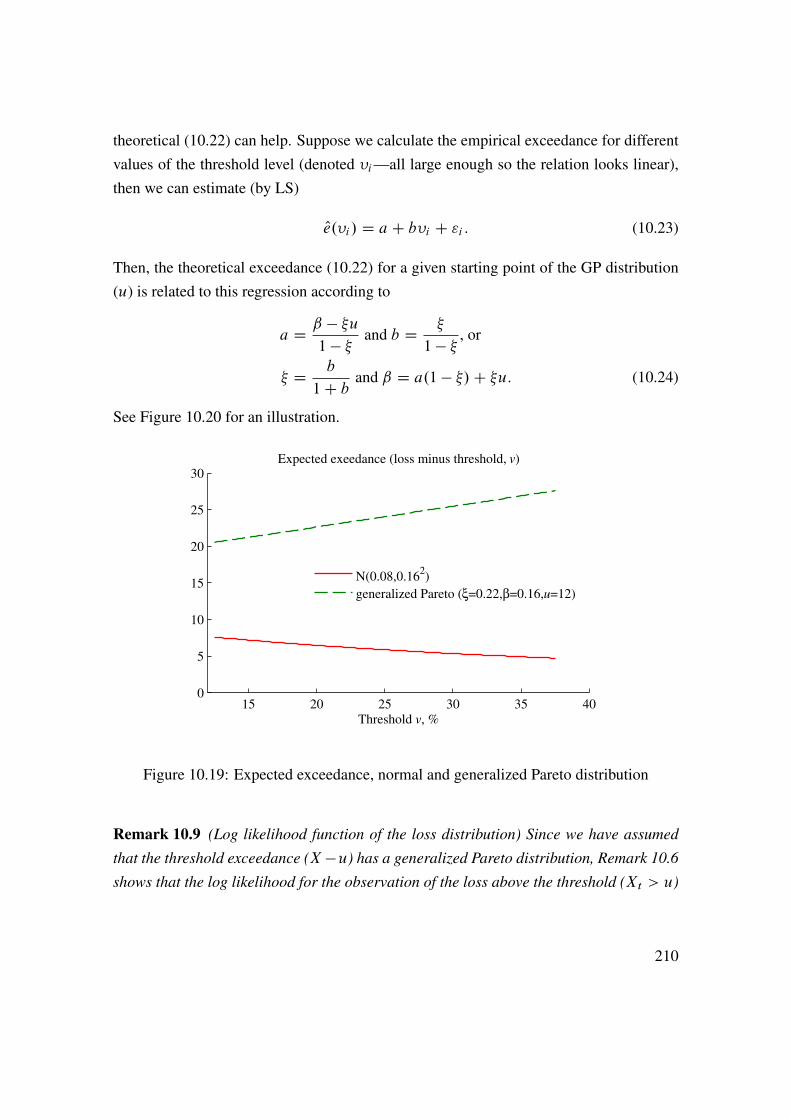
theoretical (10.22) can help. Suppose we calculate the empirical exceedance for differentvalues of the threshold level (denoted �i—all large enough so the relation looks linear),then we can estimate (by LS)
Oe.�i/ D aC b�i C "i : (10.23)
Then, the theoretical exceedance (10.22) for a given starting point of the GP distribution(u) is related to this regression according to
a D ˇ � �u1 � � and b D �
1 � � , or
� D b
1C b and ˇ D a.1 � �/C �u: (10.24)
See Figure 10.20 for an illustration.
15 20 25 30 35 400
5
10
15
20
25
30Expected exeedance (loss minus threshold, v)
Threshold v, %
N(0.08,0.162)
generalized Pareto (ξ=0.22,β=0.16,u=12)
Figure 10.19: Expected exceedance, normal and generalized Pareto distribution
Remark 10.9 (Log likelihood function of the loss distribution) Since we have assumed
that the threshold exceedance (X �u) has a generalized Pareto distribution, Remark 10.6
shows that the log likelihood for the observation of the loss above the threshold (Xt > u)
210

is
L DX
t st. Xt>u
Lt
lnLt D(� lnˇ � .1=� C 1/ ln Œ1C � .Xt � u/ =ˇ� if � ¤ 0
� lnˇ � .Xt � u/ =ˇ � D 0:
This allows us to estimate � and ˇ by maximum likelihood. Typically, u is not estimated,
but imposed a priori (based on the expected exceedance).
0 0.5 1 1.5 2 2.5
0.6
0.8
1
1.2
Expected exceedance
Threshold v, %
Loss
min
us
thre
shold
, v
(50th to 99th percentiles)
u = 1.3, ξ = 0.28, β = 0.52
1.5 2 2.5 3 3.5 40
0.05
0.1
Estimated loss distribution (pdf)
Loss, %
u = 1.3, Pr(loss>u) = 6.7%
ξ = 0.24, β = 0.57
1.5 2 2.5
1.5
2
2.5
Quantiles from estimated GPD, %
Em
pir
ical
quan
tile
s
QQ plot
(94th to 99th percentiles)Daily S&P 500 returns, 1957:1−2010:9
Figure 10.20: Results from S&P 500 data
Example 10.10 (Estimation of the generalized Pareto distribution on S&P daily returns).
Figure 10.20 (upper left panel) shows that it may be reasonable to fit a GP distribution
with a threshold u D 1:3. The upper right panel illustrates the estimated distribution,
211
while the lower left panel shows that the highest quantiles are well captured by estimated
distribution.
Bibliography
Alexander, C., 2008, Market Risk Analysis: Value at Risk Models, Wiley.
Davidson, R., and J. G. MacKinnon, 1993, Estimation and inference in econometrics,Oxford University Press, Oxford.
DeGroot, M. H., 1986, Probability and statistics, Addison-Wesley, Reading, Mas-sachusetts.
Harvey, A. C., 1989, Forecasting, structural time series models and the Kalman filter,Cambridge University Press.
Hastie, T., R. Tibshirani, and J. Friedman, 2001, The elements of statistical learning: data
mining, inference and prediction, Springer Verlag.
Lo, A. W., H. Mamaysky, and J. Wang, 2000, “Foundations of technical analysis: com-putational algorithms, statistical inference, and empirical implementation,” Journal of
Finance, 55, 1705–1765.
McNeil, A. J., R. Frey, and P. Embrechts, 2005, Quantitative risk management, PrincetonUniversity Press.
Mittelhammer, R. C., 1996, Mathematical statistics for economics and business, Springer-Verlag, New York.
Silverman, B. W., 1986, Density estimation for statistics and data analysis, Chapman andHall, London.
212
.D..3
11 Return Distributions (Multivariate)
More advanced material is denoted by a star (�). It is not required reading.
11.1 Recap of Univariate Distributions
The cdf (cumulative distribution function) measures the probability that the random vari-able Xi is below or at some numerical value xi ,
ui D Fi.xi/ D Pr.Xi � xi/: (11.1)
For instance, with an N.0; 1/ distribution, F.�1:64/ D 0:05. Clearly, the cdf valuesare between (and including) 0 and 1. The distribution of Xi is often called the marginal
distribution of Xi—to distinguish it from the joint distribution of Xi and Xj . (See belowfor more information on joint distributions.)
The pdf (probability density function) fi.xi/ is the “height” of the distribution in thesense that the cdf F.xi/ is the integral of the pdf from minus infinity to xi
Fi.xi/ DZ xi
sD�1
fi.s/ds: (11.2)
(Conversely, the pdf is the derivative of the cdf, fi.xi/ D @Fi.xi/=@xi .) The Gaussianpdf (the normal distribution) is bell shaped.
Remark 11.1 (Quantile of a distribution) The ˛ quantile of a distribution (�˛) is the value
of x such that there is a probability of ˛ of a lower value. We can solve for the quantile by
inverting the cdf, ˛ D F.�˛/ as �˛ D F �1.˛/. For instance, the 5% quantile of a N.0; 1/
distribution is �1:64 D ˚�1.0:05/, where ˚�1./ denotes the inverse of an N.0; 1/ cdf.
See Figure 11.1 for an illustration.
213
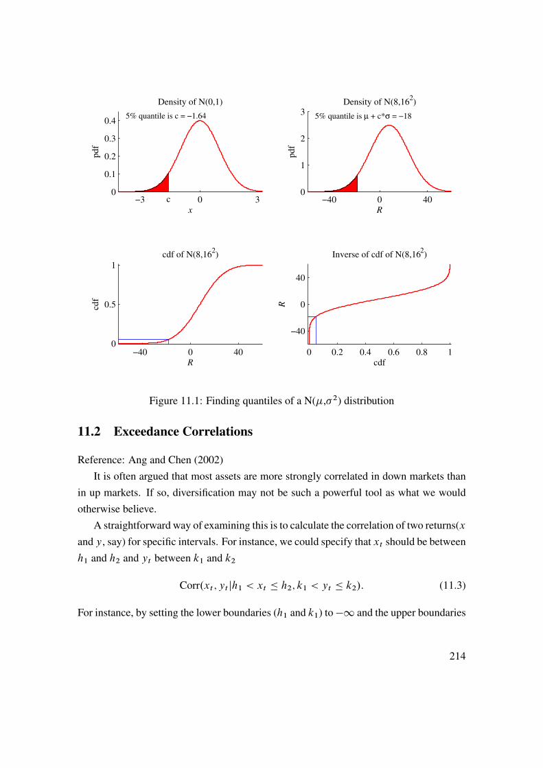
−3 0 30
0.1
0.2
0.3
0.4
Density of N(0,1)
c
5% quantile is c = −1.64
x
−40 0 400
1
2
3Density of N(8,16
2)
R
5% quantile is µ + c*σ = −18
−40 0 400
0.5
1
cdf of N(8,162)
R
cdf
0 0.2 0.4 0.6 0.8 1
−40
0
40
Inverse of cdf of N(8,162)
cdf
R
Figure 11.1: Finding quantiles of a N(�,�2) distribution
11.2 Exceedance Correlations
Reference: Ang and Chen (2002)It is often argued that most assets are more strongly correlated in down markets than
in up markets. If so, diversification may not be such a powerful tool as what we wouldotherwise believe.
A straightforward way of examining this is to calculate the correlation of two returns(xand y, say) for specific intervals. For instance, we could specify that xt should be betweenh1 and h2 and yt between k1 and k2
Corr.xt ; yt jh1 < xt � h2; k1 < yt � k2/: (11.3)
For instance, by setting the lower boundaries (h1 and k1) to�1 and the upper boundaries
214

(h2 and k2) to 0, we get the correlation in down markets.A (bivariate) normal distribution has very little probability mass at low returns, which
leads to the correlation being squeezed towards zero as we only consider data far out inthe tail. In short, the tail correlation of a normal distribution is always closer to zero thanthe correlation for all data points. This is illustrated in Figure 11.2.
In contrast, Figures 11.3–11.4 suggest (for two US portfolios) that the correlation inthe lower tail is almost as high as for all the data and considerably higher than for theupper tail. This suggests that the relation between the two returns in the tails is not welldescribed by a normal distribution. In particular, we need to use a distribution that allowsfor much stronger dependence in the lower tail. Otherwise, the diversification benefits (indown markets) are likely to be exaggerated.
0 0.1 0.2 0.3 0.4 0.50
0.1
0.2
0.3
0.4
0.5
0.6
0.7
Upper boundary (prob of lower value)
Correlation in lower tail, bivariate N(0,1) distribution
ρ=0.75
ρ=0.5
ρ=0.25
Figure 11.2: Correlation in lower tail when data is drawn from a normal distribution withcorrelation �
11.3 Beyond (Linear) Correlations
Reference: Alexander (2008) 6, McNeil, Frey, and Embrechts (2005)The standard correlation (also called Pearson’s correlation) measures the linear rela-
tion between two variables, that is, to what extent one variable can be explained by a
215

−15 −10 −5 0 5 10
−15
−10
−5
0
5
10
Returns of small value stocks, %
Ret
urn
s of
larg
e val
ue
stock
s, %
Daily US data 1979:1−2010:9
Lines mark 5th and 95th percentiles
Extreme returns of two portfolios
All
Low
Mid
High
Corr
0.64
0.68
0.40
0.51
freq
1.00
0.02
0.85
0.02
Figure 11.3: Correlation of two portfolios
0 0.1 0.2 0.3 0.4 0.50.4
0.5
0.6
0.7
0.8
Upper boundary (prob of lower value)
Lower tail correlation
small value stocks and large value stocks
Daily US data 1979:1−2010:9
0.5 0.6 0.7 0.8 0.90.4
0.5
0.6
0.7
0.8
Lower boundary (prob of lower value)
Upper tail correlation
Figure 11.4: Correlation in the tails for two portfolios
216
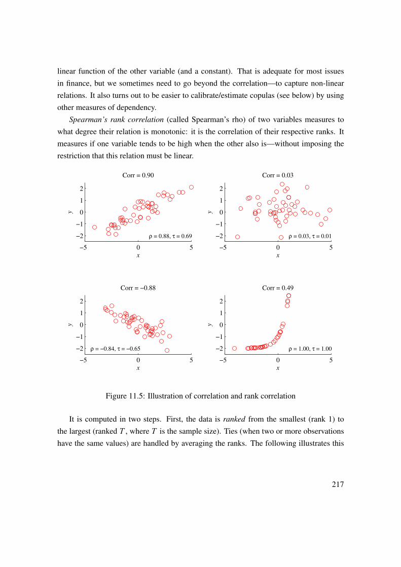
linear function of the other variable (and a constant). That is adequate for most issuesin finance, but we sometimes need to go beyond the correlation—to capture non-linearrelations. It also turns out to be easier to calibrate/estimate copulas (see below) by usingother measures of dependency.
Spearman’s rank correlation (called Spearman’s rho) of two variables measures towhat degree their relation is monotonic: it is the correlation of their respective ranks. Itmeasures if one variable tends to be high when the other also is—without imposing therestriction that this relation must be linear.
−5 0 5
−2
−1
0
1
2
Corr = 0.90
ρ = 0.88, τ = 0.69
x
y
−5 0 5
−2
−1
0
1
2
Corr = 0.03
ρ = 0.03, τ = 0.01
x
y
−5 0 5
−2
−1
0
1
2
Corr = −0.88
ρ = −0.84, τ = −0.65
x
y
−5 0 5
−2
−1
0
1
2
Corr = 0.49
ρ = 1.00, τ = 1.00
x
y
Figure 11.5: Illustration of correlation and rank correlation
It is computed in two steps. First, the data is ranked from the smallest (rank 1) tothe largest (ranked T , where T is the sample size). Ties (when two or more observationshave the same values) are handled by averaging the ranks. The following illustrates this
217

for two variablesxt rank.xt/ yt rank.yt/2 2:5 7 2
10 4 8 3
�3 1 2 1
2 2:5 10 4
(11.4)
In the second step, simply estimate the correlation of the ranks of two variables
Spearman’s � D CorrŒrank.xt/; rank.yt/�: (11.5)
Clearly, this correlation is between �1 and 1. (There is an alternative way of calculatingthe rank correlation based on the difference of the ranks, dt Drank.xt/�rank.yt/, � D1 � 6˙T
tD1d2t =.T
3 � T /. It gives the same result if there are no tied ranks.) See Figure11.5 for an illustration.
The rank correlation can be tested by using the fact that under the null hypothesis therank correlation is zero. We then get
pT � 1 O�!d N.0; 1/: (11.6)
(For samples of 20 to 40 observations, it is often recommended to usep.T � 2/=.1 � O�2/ O�
which has an tT�2 distribution.)
Remark 11.2 (Spearman’s � for a distribution�) If we have specified the joint distribu-
tion of the random variablesX and Y , then we can also calculate the implied Spearman’s
� (sometimes only numerically) as CorrŒFX.X/; FY .Y /� where FX.X/ is the cdf ofX and
FY .Y / of Y .
Kendall’s rank correlation (called Kendall’s � ) is similar, but is based on compar-ing changes of xt (compared to x1; : : : xt�1) with the corresponding changes of yt . Forinstance, with three data points (.x1; y1/; .x2; y2/; .x3; y3/) we first calculate
Changes of x Changes of yx2 � x1 y2 � y1x3 � x1 y3 � y1x3 � x2 y3 � y2;
(11.7)
218
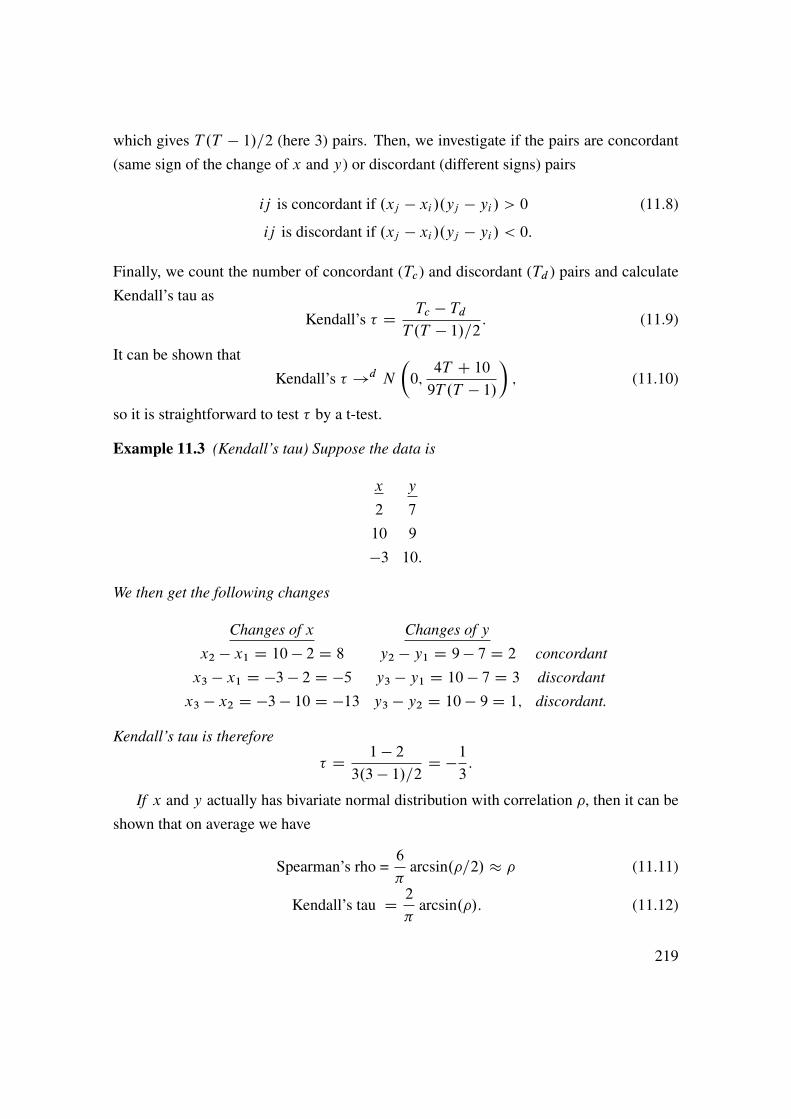
which gives T .T � 1/=2 (here 3) pairs. Then, we investigate if the pairs are concordant(same sign of the change of x and y) or discordant (different signs) pairs
ij is concordant if .xj � xi/.yj � yi/ > 0 (11.8)
ij is discordant if .xj � xi/.yj � yi/ < 0:
Finally, we count the number of concordant (Tc) and discordant (Td ) pairs and calculateKendall’s tau as
Kendall’s � D Tc � TdT .T � 1/=2: (11.9)
It can be shown thatKendall’s � !d N
�0;
4T C 109T .T � 1/
�; (11.10)
so it is straightforward to test � by a t-test.
Example 11.3 (Kendall’s tau) Suppose the data is
x y
2 7
10 9
�3 10:
We then get the following changes
Changes of x Changes of y
x2 � x1 D 10 � 2 D 8 y2 � y1 D 9 � 7 D 2 concordant
x3 � x1 D �3 � 2 D �5 y3 � y1 D 10 � 7 D 3 discordant
x3 � x2 D �3 � 10 D �13 y3 � y2 D 10 � 9 D 1; discordant.
Kendall’s tau is therefore
� D 1 � 23.3 � 1/=2 D �
1
3:
If x and y actually has bivariate normal distribution with correlation �, then it can beshown that on average we have
Spearman’s rho =6
�arcsin.�=2/ � � (11.11)
Kendall’s tau D 2
�arcsin.�/: (11.12)
219

In this case, all three measures give similar messages (although the Kendall’s tau tends tobe lower than the linear correlation and Spearman’s rho). This is illustrated in Figure 11.6.Clearly, when data is not normally distributed, then these measures can give distinctlydifferent answers.
0 0.2 0.4 0.6 0.8 10
0.2
0.4
0.6
0.8
1
Correlation
ρ and τ as a function of the linear correlation (Gaussian distribution)
Spearman’s ρ
Kendall’s τ
Figure 11.6: Spearman’s rho and Kendall’s tau if data has a bivariate normal distribution
A joint ˛-quantile exceedance probability measures how often two random variables(x and y, say) are both above their ˛ quantile. Similarly, we can also define the probabilitythat they are both below their ˛ quantile
G˛ D Pr.x � �x;˛; y � �y;˛/; (11.13)
�x;˛ and �y;˛ are ˛-quantile of the x- and y-distribution respectively.In practice, this can be estimated from data by first finding the empirical ˛-quantiles
( O�x;˛ and O�y;˛) by simply sorting the data and then picking out the value of observation˛T of this sorted list (do this individually for x and y). Then, calculate the estimate
OG˛ D 1
T
XT
tD1ıt ; where ıt D
(1 if xt � O�x;˛ and yt � O�y;˛
0 otherwise.(11.14)
See Figure 11.7 for an illustration based on a joint normal distribution.
220

0 20 40 60 80 1000
50
100
Prob of lower value, %
%Pr(x<quantile,y<quantile), Gauss
corr = 0.25
corr = 0.5
0 2 4 6 8 100
5
10
Prob of lower value, %
%
Pr(x<quantile,y<quantile), Gauss
Figure 11.7: Probability of joint low returns, bivariate normal distribution
11.4 Copulas
Reference: McNeil, Frey, and Embrechts (2005), Alexander (2008) 6, Jondeau, Poon, andRockinger (2007) 6
Portfolio choice and risk analysis depend crucially on the joint distribution of assetreturns. Emprical evidence suggest that many returns have non-normal distribution, es-pecially when we focus on the tails. There are several ways of estimating complicated(non-normal) distributions: using copulas is one. This approach has the advantage thatit proceeds in two steps: first we estimate the marginal distribution of each returns sepa-rately, then we model the comovements by a copula.
11.4.1 Multivariate Distributions and Copulas
Any pdf can also be written as
f1;2.x1; x2/ D c.u1; u2/f1.x1/f2.x2/; with ui D Fi.xi/; (11.15)
where c./ is a copula density function and ui D Fi.xi/ is the cdf value as in (11.1). Theextension to three or more random variables is straightforward.
Equation (11.15) means that if we know the joint pdf f1;2.x1; x2/—and thus also thecdfs F1.x1/ and F2.x2/—then we can figure out what the copula density function mustbe. Alternatively, if we know the pdfs f1.x1/ and f2.x2/—and thus also the cdfs F1.x1/and F2.x2/—and the copula function, then we can construct the joint distribution. (Thisis called Sklar’s theorem.) This latter approach will turn out to be useful.
221

The correlation of x1 and x2 depends on both the copula and the marginal distribu-tions. In contrast, both Spearman’s rho and Kendall’s tau are determined by the copulaonly. They therefore provide a way of calibrating/estimating the copula without having toinvolve the marginal distributions directly.
Example 11.4 (Independent X and Y ) If X and Y are independent, then we know that
f1;2.x1; x2/ D f1.x1/f2.x2/, so the copula density function is just a constant equal to
one.
Remark 11.5 (Joint cdf) A joint cdf of two random variables (X1 and X2) is defined as
F1;2.x1; x2/ D Pr.X1 � x1 and X2 � x2/:
This cdf is obtained by integrating the joint pdf f1;2.x1; x2/ over both variables
F1;2.x1; x2/ DZ x1
sD�1
Z x2
tD�1
f1;2.s; t/dsdt:
(Conversely, the pdf is the mixed derivative of the cdf, f1;2.x1; x2/ D @2F1;2.x1; x2/=@x1@x2.)See Figure 11.8 for an illustration.
Remark 11.6 (From joint to univariate pdf) The pdf of x1 (also called the marginal pdf
of x1) can be calculate from the joint pdf as f1.x1/ DR1x2D�1
f1;2.x1; x2/dx2.
−2
0
2
−20
20
0.1
0.2
x
pdf of bivariate normal distribution, corr=0.8
y−2
0
2
−20
20
0.5
1
x
cdf of bivariate normal distribution, corr=0.8
y
Figure 11.8: Bivariate normal distributions
222

Remark 11.7 (Joint pdf and copula density, n variables) For n variables (11.15) gener-
alizes to
f1;2;:::;n.x1; x2; : : : ; xn/ D c.u1; u2; : : : ; un/f1.x1/f2.x2/ : : : fn.xn/; with ui D Fi.xi/;
Remark 11.8 (Cdfs and copulas�) The joint cdf can be written as
F1;2.x1; x2/ D C ŒF1.x1/; F2.x2/�;
where C./ is the unique copula function. Taking derivatives gives (11.15) where
c.u1; u2/ D @2C.u1; u2/
@u1@u2:
Notice the derivatives are with respect to ui D Fi.xi/, not xi . Conversely, integrating the
density over both u1 and u2 gives the copula function C./.
11.4.2 The Gaussian and Other Copula Densities
The Gaussian copula density function is
c.u1; u2/ D 1p1 � �2
exp���
2�21 � 2��1�2 C �2�222.1 � �2/
�, with �i D ˚�1.ui/; (11.16)
where˚�1./ is the inverse of anN.0; 1/ distribution. Notice that when using this functionin (11.15) to construct the joint pdf, we have to first calculate the cdf values ui D Fi.xi/from the univariate distribution of xi (which may be non-normal) and then calculatethe quantiles of those according to a standard normal distribution �i D ˚�1.ui/ D˚�1ŒFi.xi/�.
It can be shown that assuming that the marginal pdfs (f1.x1/ and f2.x2/) are normaland then combining with the Gaussian copula density recovers a bivariate normal dis-tribution. However, the way we typically use copulas is to assume (and estimate) someother type of univariate distribution, for instance, with fat tails—and then combine with a(Gaussian) copula density to create the joint distribution. See Figure 11.9 for an illustra-tion.
A zero correlation (� D 0) makes the copula density (11.16) equal to unity—so thejoint density is just the product of the marginal densities. A positive correlation makes thecopula density high when both x1 and x2 deviate from their means in the same direction.
223

The easiest way to calibrate a Gaussian copula is therefore to set
� D Spearman’s rho, (11.17)
as suggested by (11.11).Alternatively, the � parameter can calibrated to give a joint probability of both x1
and x2 being lower than some quantile as to match data: see (11.14). The values of thisprobability (according to a copula) is easily calculated by finding the copula function(essentially the cdf) corresponding to a copula density. Some results are given in remarksbelow. See Figure 11.7 for results from a Gaussian copula. This figure shows that ahigher correlation implies a larger probability that both variables are very low—but thatthe probabilities quickly become very small as we move towards lower quantiles (lowerreturns).
Remark 11.9 (The Gaussian copula function�) The distribution function corresponding
to the Gaussian copula density (11.16) is obtained by integrating over both u1 and u2 and
the value is C.u1; u2I �/ D ˚�.�1; �2/ where �i is defined in (11.16) and ˚� is the bi-
variate normal cdf for N
"0
0
#;
"1 �
� 1
#!. Most statistical software contains numerical
returns for calculating this cdf.
Remark 11.10 (Multivariate Gaussian copula density�) The Gaussian copula density for
n variables is
c.u/ D 1pjRj
exp��12� 0.R�1 � In/�
�;
where R is the correlation matrix with determinant jRj and � is a column vector with
�i D ˚�1.ui/ as the i th element.
The Gaussian copula is useful, but it has the drawback that it is symmetric—so thedownside and the upside look the same. This is at odds with evidence from many financialmarkets that show higher correlations across assets in down markets. The Clayton copula
density is therefore an interesting alternative
c.u1; u2/ D .�1C u�˛1 C u�˛2 /�2�1=˛.u1u2/�˛�1.1C ˛/; (11.18)
where ˛ ¤ 0. When ˛ > 0, then correlation on the downside is much higher than on theupside (where it goes to zero as we move further out the tail).
224

See Figure 11.9 for an illustration.For the Clayton copula we have
Kendall’s � D ˛
˛ C 2 , so (11.19)
˛ D 2�
1 � � : (11.20)
The easiest way to calibrate a Clayton copula is therefore to set the parameter ˛ accordingto (11.20).
Figure 11.10 illustrates how the probability of both variables to be below their respec-tive quantiles depend on the ˛ parameter. These parameters are comparable to the thosefor the correlations in Figure 11.7 for the Gaussian copula, see (11.11)–(11.12). The figureare therefore comparable—and the main point is that Clayton’s copula gives probabilitiesof joint low values (both variables being low) that do not decay as quickly as according tothe Gaussian copulas. Intuitively, this means that the Clayton copula exhibits much higher“correlations” in the lower tail than the Gaussian copula does—although they imply thesame overall correlation. That is, according to the Clayton copula more of the overallcorrelation of data is driven by synchronized movements in the left tail. This could beinterpreted as if the correlation is higher in market crashes than during normal times.
Remark 11.11 (Multivariate Clayton copula density�) The Clayton copula density for n
variables is
c.u/ D �1 � nCPniD1u
�˛i
��n�1=˛ �QniD1ui
��˛�1 �QniD1Œ1C .i � 1/˛�
�:
Remark 11.12 (Clayton copula function�) The copula function (the cdf) corresponding
to (11.18) is
C.u1; u2/ D .�1C u�˛1 C u�˛2 /�1=˛:
The following steps summarize how the copula is used to construct the multivariatedistribution.
1. Construct the marginal pdfs fi.xi/ and thus also the marginal cdfs Fi.xi/. For in-stance, this could be done by fitting a distribution with a fat tail. With this, calculatethe cdf values for the data ui D Fi.xi/ as in (11.1).
225
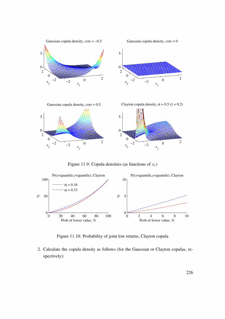
−2 0 2−20
2
0
5
x1
Gaussian copula density, corr = −0.5
x2
−2 0 2−20
2
0
5
Gaussian copula density, corr = 0
x1
x2
−2 0 2−20
2
0
5
x1
Gaussian copula density, corr = 0.5
x2
−2 0 2−20
2
0
5
x1
Clayton copula density, α = 0.5 (τ = 0.2)
x2
Figure 11.9: Copula densities (as functions of xi )
0 20 40 60 80 1000
50
100
Prob of lower value, %
%
Pr(x<quantile,y<quantile), Clayton
α = 0.16
α = 0.33
0 2 4 6 8 100
5
10
Prob of lower value, %
%
Pr(x<quantile,y<quantile), Clayton
Figure 11.10: Probability of joint low returns, Clayton copula
2. Calculate the copula density as follows (for the Gaussian or Clayton copulas, re-spectively):
226

(a) for the Gaussian copula (11.16)
i. assume (or estimate/calibrate) a correlation � to use in the Gaussian cop-ula
ii. calculate �i D ˚�1.ui/, where ˚�1./ is the inverse of a N.0; 1/ distribu-tion
iii. combine to get the copula density value c.u1; u2/
(b) for the Clayton copula (11.18)
i. assume (or estimate/calibrate) an ˛ to use in the Clayton copula (typicallybased on Kendall’s � as in (11.20))
ii. calculate the copula density value c.u1; u2/
3. Combine the marginal pdfs and the copula density as in (11.15), f1;2.x1; x2/ Dc.u1; u2/f1.x1/f2.x2/, where ui D Fi.xi/ is the cdf value according to the marginaldistribution of variable i .
See Figures 11.11–11.12 for illustrations.
Remark 11.13 (Tail Dependence�) The measure of lower tail dependence starts by find-
ing the probability that X1 is lower than its qth quantile (X1 � F �11 .q/) given that X2 is
lower than its qth quantile (X2 � F �12 .q/)
�l D PrŒX1 � F �11 .q/jX2 � F �12 .q/�;
and then takes the limit as the quantile goes to zero
�l D limq!0 PrŒX1 � F �11 .q/jX2 � F �12 .q/�:
It can be shown that a Gaussian copula gives zero or very weak tail dependence,
unless the correlation is 1. It can also be shown that the lower tail dependence of the
Clayton copula is
�l D 2�1=˛ if ˛ > 0
and zero otherwise.
227

Joint pdf, Gaussian copula, corr = −0.5
x1
x2
Notice: marginal distributions are N(0,1)
−2 −1 0 1 2
−2
−1
0
1
2
Joint pdf, Gaussian copula, corr = 0
x1
x2
−2 −1 0 1 2
−2
−1
0
1
2
Joint pdf, Gaussian copula, corr = 0.5
x1
x2
−2 −1 0 1 2
−2
−1
0
1
2
Joint pdf, Clayton copula, α = 0.5
x1
x2
−2 −1 0 1 2
−2
−1
0
1
2
Figure 11.11: Contours of bivariate pdfs
11.5 Joint Tail Distribution
The methods for estimating the (marginal, that is, for one variable at a time) distributionof the lower tail can be combined with a copula to model the joint tail distribution. Inparticular, combining the generalized Pareto distribution (GPD) with the Clayton copulaprovides a flexible way.
This can be done by first modelling the loss (Xt D �Rt ) beyond some threshold (u),that is, the variableXt�u with the GDP. To get a distribution of the return, we simply usethe fact that pdfR.�z/ D pdfX.z/ for any value z. Then, in a second step we calibrate thecopula by using Kendall’s � for the subsample when both returns are less than u. Figures11.13–11.15 provide an illustration.
Remark 11.14 Figure 11.13 suggests that the joint occurrence (of these two assets) of
228
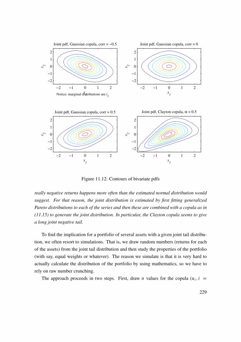
Joint pdf, Gaussian copula, corr = −0.5
x1
x2
Notice: marginal distributions are t5
−2 −1 0 1 2
−2
−1
0
1
2
Joint pdf, Gaussian copula, corr = 0
x1
x2
−2 −1 0 1 2
−2
−1
0
1
2
Joint pdf, Gaussian copula, corr = 0.5
x1
x2
−2 −1 0 1 2
−2
−1
0
1
2
Joint pdf, Clayton copula, α = 0.5
x1
x2
−2 −1 0 1 2
−2
−1
0
1
2
Figure 11.12: Contours of bivariate pdfs
really negative returns happens more often than the estimated normal distribution would
suggest. For that reason, the joint distribution is estimated by first fitting generalized
Pareto distributions to each of the series and then these are combined with a copula as in
(11.15) to generate the joint distribution. In particular, the Clayton copula seems to give
a long joint negative tail.
To find the implication for a portfolio of several assets with a given joint tail distribu-tion, we often resort to simulations. That is, we draw random numbers (returns for eachof the assets) from the joint tail distribution and then study the properties of the portfolio(with say, equal weights or whatever). The reason we simulate is that it is very hard toactually calculate the distribution of the portfolio by using mathematics, so we have torely on raw number crunching.
The approach proceeds in two steps. First, draw n values for the copula (ui ; i D
229

0 20 40 60 80 1000
50
100
Prob of lower value, %
%
Daily US data 1979:1−2010:9
small value stocks and large value stocks
Prob(both returns < quantile)
Data
estimated N()
0 2 4 6 8 100
1
2
3
4
5
Prob of lower value, %
%
Prob(both returns < quantile), zoomed in
Figure 11.13: Probability of joint low returns
1; : : : ; n). Second, calculate the random number (“return”) by inverting the cdf ui DFi.xi/ in (11.15) as
xi D F �1i .ui/; (11.21)
where F �1i ./ is the inverse of the cdf.
Remark 11.15 (To draw n random numbers from a Gaussian copula) First, draw n num-
bers from an N.0;R/ distribution, where R is the correlations matrix. Second, calculate
ui D ˚.xi/, where ˚ is the cdf of a standard normal distribution.
Remark 11.16 (To draw n random numbers from a Clayton copula) First, draw xi for
i D 1; : : : ; n from a uniform distribution (between 0 and 1). Second, draw v from a
gamma(1=˛; 1) distribution. Third, calculate ui D Œ1 � ln.xi/=v��1=˛ for i D 1; : : : ; n.
These ui values are the marginal cdf values.
Remark 11.17 (Inverting a normal and a generalised Pareto cdf) Must numerical soft-
ware packages contain a routine for investing a normal cdf. My lecture notes on the
Generalised Pareto distribution shows how to invert that distribution.
Such simulations can be used to quickly calculate the VaR and other risk measuresfor different portfolios. A Clayton copula with a high ˛ parameter (and hence a highKendall’s � ) has long lower tail with highly correlated returns: when asset takes a dive,
230

1 2 3 4 50
0.05
0.1
0.15
0.2
Loss distribution, small value stocks
Loss, %
u = 0.5, Pr(loss>u) = 11.3%
ξ = 0.29, β = 0.44
Daily US data 1979:1−2010:9
1 2 3 4 50
0.05
0.1
0.15
0.2
Loss distribution, large value stocks
Loss, %
u = 0.5, Pr(loss>u) = 23.7%
ξ = 0.19, β = 0.63
−5 −4 −3 −2 −10
0.05
0.1
0.15
0.2
Return distribution, small value stocks
Return, %
(Only lower tail is shown)
−5 −4 −3 −2 −10
0.05
0.1
0.15
0.2
Return distribution, large value stocks
Return, %
(Only lower tail is shown)
Figure 11.14: Estimation of marginal loss distributions
other assets are also likely to decrease. That is, the correlation in the lower tail of thereturn distribution is high, which will make the VaR high.
Figures 11.16–11.17 give an illustration of how the movements in the lower get moresynchronised as the ˛ parameter in the Clayton copula increases.
Bibliography
Alexander, C., 2008, Market Risk Analysis: Practical Financial Econometrics, Wiley.
Ang, A., and J. Chen, 2002, “Asymmetric correlations of equity portfolios,” Journal of
Financial Economics, 63, 443–494.
Jondeau, E., S.-H. Poon, and M. Rockinger, 2007, Financial Modeling under Non-
Gaussian Distributions, Springer.
231

Joint pdf, independent copula
small value stocks
larg
e val
ue
stock
s
−4 −3 −2 −1−4
−3
−2
−1
Joint pdf, Gaussian copula
Spearman’s ρ = 0.49
small value stocks
larg
e val
ue
stock
s
−4 −3 −2 −1−4
−3
−2
−1
Joint pdf, Clayton copula
Kendall’s τ = 0.35, α = 1.06
small value stocks
larg
e val
ue
stock
s
−4 −3 −2 −1−4
−3
−2
−1
Daily US data 1979:1−2010:9
The marginal distributions of the losses
are estimated GP distributions
Figure 11.15: Joint pdfs with different copulas
McNeil, A. J., R. Frey, and P. Embrechts, 2005, Quantitative risk management, PrincetonUniversity Press.
232
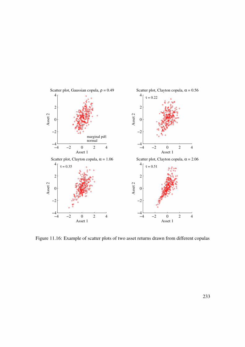
−4 −2 0 2 4−4
−2
0
2
4
Scatter plot, Gaussian copula, ρ = 0.49
Asset 1
Ass
et 2
marginal pdf: normal
−4 −2 0 2 4−4
−2
0
2
4
Scatter plot, Clayton copula, α = 0.56
Asset 1
Ass
et 2
τ = 0.22
−4 −2 0 2 4−4
−2
0
2
4
Scatter plot, Clayton copula, α = 1.06
Asset 1
Ass
et 2
τ = 0.35
−4 −2 0 2 4−4
−2
0
2
4
Scatter plot, Clayton copula, α = 2.06
Asset 1
Ass
et 2
τ = 0.51
Figure 11.16: Example of scatter plots of two asset returns drawn from different copulas
233
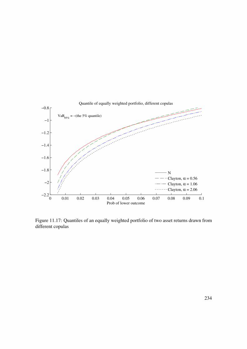
0 0.01 0.02 0.03 0.04 0.05 0.06 0.07 0.08 0.09 0.1−2.2
−2
−1.8
−1.6
−1.4
−1.2
−1
−0.8Quantile of equally weighted portfolio, different copulas
Prob of lower outcome
VaR95%
= −(the 5% quantile)
N
Clayton, α = 0.56
Clayton, α = 1.06
Clayton, α = 2.06
Figure 11.17: Quantiles of an equally weighted portfolio of two asset returns drawn fromdifferent copulas
234
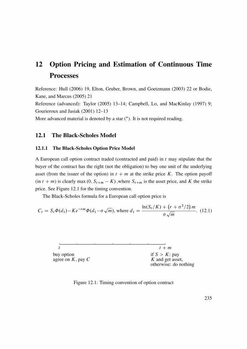
12 Option Pricing and Estimation of Continuous TimeProcesses
Reference: Hull (2006) 19, Elton, Gruber, Brown, and Goetzmann (2003) 22 or Bodie,Kane, and Marcus (2005) 21Reference (advanced): Taylor (2005) 13–14; Campbell, Lo, and MacKinlay (1997) 9;Gourieroux and Jasiak (2001) 12–13More advanced material is denoted by a star (�). It is not required reading.
12.1 The Black-Scholes Model
12.1.1 The Black-Scholes Option Price Model
A European call option contract traded (contracted and paid) in t may stipulate that thebuyer of the contract has the right (not the obligation) to buy one unit of the underlyingasset (from the issuer of the option) in t C m at the strike price K. The option payoff(in t Cm) is clearly max .0; StCm �K/ ;where StCm is the asset price, and K the strikeprice. See Figure 12.1 for the timing convention.
The Black-Scholes formula for a European call option price is
Ct D St˚.d1/�Ke�rm˚.d1��pm/, where d1 D
ln.St=K/C�r C �2=2�m
�pm
: (12.1)
t t C m
buy optionagree on K, pay C
if S > K: payK and get asset,otherwise: do nothing
Figure 12.1: Timing convention of option contract
235

−3 −2 −1 0 1 2 30
0.1
0.2
0.3
0.4
Pdf of N(0,1)
x
Pr(x ≤ −1): 0.16
−3 −2 −1 0 1 2 30
0.1
0.2
0.3
0.4
Pdf of N(0,1)
x
Pr(x ≤ 0.5): 0.69
−3 −2 −1 0 1 2 30
0.5
1
Cdf of N(0,1)
x
Figure 12.2: Pdf and cdf of N(0,1)
where ˚./ is the cumulative distribution function for a variable distributed as N(0,1). Forinstance, ˚.2/ is the probability that y � 2 — see Figure 12.2. In this equation, S0 is theprice of the underlying asset in period t , and r is the continuously compounded interestrate (on an annualized basis).
Some basic properties of the model are illustrated in Figure 12.3. In particular, thecall option price is increasing in the volatility and decreasing in the strike price.
The B-S formula can be derived from several stochastic processes of the underlyingasset price (discussed below), but they all imply that the distribution of log asset price int C m (conditional on the information in t ) is normal with some mean ˛ (not importantfor the option price) and the variance m�2
lnStCm � N.˛;m�2/: (12.2)
236
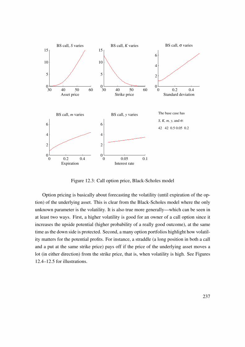
30 40 50 600
5
10
15BS call, S varies
Asset price
30 40 50 600
5
10
15BS call, K varies
Strike price
0 0.2 0.40
2
4
6
BS call, σ varies
Standard deviation
0 0.2 0.40
2
4
6
BS call, m varies
Expiration
0 0.05 0.10
2
4
6
BS call, y varies
Interest rate
The base case has
S, K, m, y, and σ:
42 42 0.5 0.05 0.2
Figure 12.3: Call option price, Black-Scholes model
Option pricing is basically about forecasting the volatility (until expiration of the op-tion) of the underlying asset. This is clear from the Black-Scholes model where the onlyunknown parameter is the volatility. It is also true more generally—which can be seen inat least two ways. First, a higher volatility is good for an owner of a call option since itincreases the upside potential (higher probability of a really good outcome), at the sametime as the down side is protected. Second, a many option portfolios highlight how volatil-ity matters for the potential profits. For instance, a straddle (a long position in both a calland a put at the same strike price) pays off if the price of the underlying asset moves alot (in either direction) from the strike price, that is, when volatility is high. See Figures12.4–12.5 for illustrations.
237

20 30 40 50 60 700
0.02
0.04
0.06
Distribution of future asset price
Asset price
K = 42Std = 0.14
20 30 40 50 60 700
0.02
0.04
0.06
Distribution of future asset price
Asset price
K = 42Std = 0.21
Figure 12.4: Distribution of future stock price
0
K
Stock price
Profit of straddle, call + put
Call(K)
Put(K)
Straddle
Figure 12.5: Profit of straddle portfolio
12.1.2 Implied Volatility
The pricing formula (12.1) contains only one unknown parameter: the standard deviation� in the distribution of lnStCm, see (12.2). With data on the option price, spot price,the interest rate, and the strike price, we can solve for standard deviation: the implied
238
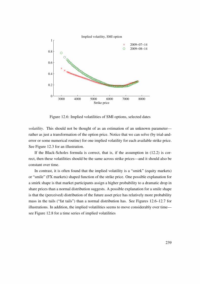
3000 4000 5000 6000 7000 80000
0.2
0.4
0.6
0.8
1
Strike price
Implied volatility, SMI option
2009−07−14
2009−08−14
Figure 12.6: Implied volatilities of SMI options, selected dates
volatility. This should not be thought of as an estimation of an unknown parameter—rather as just a transformation of the option price. Notice that we can solve (by trial-and-error or some numerical routine) for one implied volatility for each available strike price.See Figure 12.3 for an illustration.
If the Black-Scholes formula is correct, that is, if the assumption in (12.2) is cor-rect, then these volatilities should be the same across strike prices—and it should also beconstant over time.
In contrast, it is often found that the implied volatility is a “smirk” (equity markets)or “smile” (FX markets) shaped function of the strike price. One possible explanation fora smirk shape is that market participants assign a higher probability to a dramatic drop inshare prices than a normal distribution suggests. A possible explanation for a smile shapeis that the (perceived) distribution of the future asset price has relatively more probabilitymass in the tails (“fat tails”) than a normal distribution has. See Figures 12.6–12.7 forillustrations. In addition, the implied volatilities seems to move considerably over time—see Figure 12.8 for a time series of implied volatilities
239
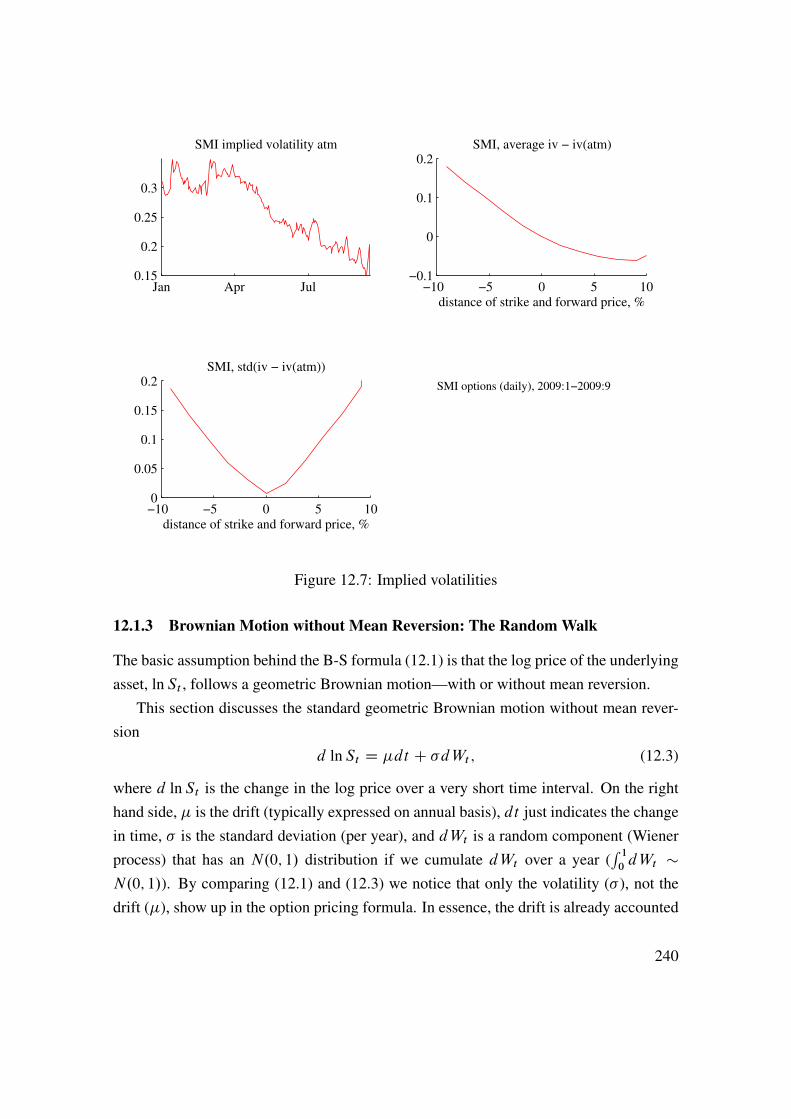
Jan Apr Jul0.15
0.2
0.25
0.3
SMI implied volatility atm
−10 −5 0 5 10−0.1
0
0.1
0.2SMI, average iv − iv(atm)
distance of strike and forward price, %
−10 −5 0 5 100
0.05
0.1
0.15
0.2SMI, std(iv − iv(atm))
distance of strike and forward price, %
SMI options (daily), 2009:1−2009:9
Figure 12.7: Implied volatilities
12.1.3 Brownian Motion without Mean Reversion: The Random Walk
The basic assumption behind the B-S formula (12.1) is that the log price of the underlyingasset, lnSt , follows a geometric Brownian motion—with or without mean reversion.
This section discusses the standard geometric Brownian motion without mean rever-sion
d lnSt D �dt C �dWt ; (12.3)
where d lnSt is the change in the log price over a very short time interval. On the righthand side, � is the drift (typically expressed on annual basis), dt just indicates the changein time, � is the standard deviation (per year), and dWt is a random component (Wienerprocess) that has an N.0; 1/ distribution if we cumulate dWt over a year (
R 10dWt �
N.0; 1/). By comparing (12.1) and (12.3) we notice that only the volatility (� ), not thedrift (�), show up in the option pricing formula. In essence, the drift is already accounted
240

1990 1992 1994 1996 1998 2000 2002 2004 2006 2008 2010 2012
10
20
30
40
50
60
70
80
CBOE volatility index (VIX)
Kuwait
Gulf war
Stock market crash
Asia
LTCM/Russia
9/11
pharma
Iraq
Higher rates
sub prime
Lehman
Greece
Fukushima
Figure 12.8: CBOE VIX, summary measure of implied volatities (30 days) on US stockmarkets
for by the current spot price in the option pricing formula (as the spot price certainlydepends on the expected drift of the asset price).
Remark 12.1 (Alternative stock price process�) If we instead of (12.3) assume the pro-
cess dSt D Q�Stdt C�StdWt , then we get the same option price. The reason is that Itô’s
lemma tells us that (12.3) implies this second process with Q� D �C�2=2. The difference
is only in terms of the drift, which does not show up (directly, at least) in the B-S formula.
Remark 12.2 ((12.3) as a limit of a discrete time process�) (12.3) can be thought of as
the limit of the discrete time process lnSt � lnSt�h D �hC�"t (where "t is white noise)
as the time interval h becomes very small.
We can only observe the value of the asset price at a limited number of times, so weneed to understand what (12.3) implies for discrete time intervals. It is straightforward toshow that (12.3) implies that we have normally distributed changes and that the changes
241

are uncorrelated (for non-overlapping data)
ln.St=St�h/ � N.�h; �2h/ (12.4)
CovŒln.St=St�h/; ln.StCh=St/� D 0: (12.5)
Notice that both the drift and the variance scale linearly with the horizon h. The reasonis, or course, that the growth rates (even for the infinitesimal horizon) are iid.
Remark 12.3 (iid random variable in discrete time) Suppose xt has the constant mean �
and a variance �2. Then E.xtCxt�1/ D 2� and Var.xtCxt�1/ D 2�2C2Cov.xt ; xt�1/.If xt is iid, then the covariance is zero, so Var.xt C xt�1/ D 2�2. In this case, both mean
and variance scale linearly with the horizon.
12.1.4 Brownian Motion with Mean Reversion�
The mean reverting Ornstein-Uhlenbeck process is
d lnSt D �.� � lnSt/dt C �dWt , with � > 0: (12.6)
This process makes lnSt revert back to the mean �, and the mean reversion is faster if �is large. It is used in, for instance, the Vasicek model of interest rates.
To estimate the parameters in (12.6) on real life data, we (once again) have to under-stand what the model implies for discretely sampled data. It can be shown that it impliesa discrete time AR(1)
lnSt D ˛ C � lnSt�h C "t , with (12.7)
� D e��h; ˛ D �.1 � �/, and "t � N�0; �2.1 � �2/=.2�/� : (12.8)
We know that the maximum likelihood estimator (MLE) of the discrete AR(1) is leastsquares combined with the traditional estimator of the residual variance. MLE has thefurther advantage of being invariant to parameter transformations, which here means thatthe MLE of �;� and �2 can be backed out from the LS estimates of �; ˛ and Var."t ) byusing (12.8).
Example 12.4 Suppose �;� and �2 are 2, 0, and 0.25 respectively—and the periods are
years (so one unit of time corresponds to a year) . Equations (12.7)–(12.8) then gives the
242

0 h 2h T D nh
0 h 2h T D nh
Figure 12.9: Two different samplings with same time span T
following AR(1) for weekly (h D 1=52) data
lnSt D 0:96 lnSt�h C "t with Var."t/ � 0:24:
12.2 Estimation of the Volatility of a Random Walk Process
This section discusses different ways of estimating the volatility. We will assume that wehave data for observations in � D 1; 2; ::; n. This could be 5-minute intervals, days orweeks or whatever. Let the time between � and � C 1 be h (years). The sample thereforestretches over T D nh periods (years). For instance, for daily data h D 1=365 (orpossibly something like 1=252 if only trading days are counted). Instead, with weeklydata h D 1=52. See Figure 12.9 for an illustration.
12.2.1 Standard Approach
We first estimate the variance for the sampling frequency we have, and then convert to theannual frequency.
According to (12.4) the growth rates, ln.St=St�h/, are iid over any sampling fre-quency. To simplify the notation, let y� D ln.S�=S��1/ be the observed growth rates.The classical estimator of the variance of an iid data series is
Os2 DXn
�D1.y� � Ny/2 =n, where (12.9)
Ny DXn
�D1y�=n: (12.10)
(This is also the maximum likelihood estimator.) To annualize these numbers, use
O�2 D Os2=h, and O� D Ny=h: (12.11)
243

Example 12.5 If . Ny; Os2/ D .0:001; 0:03/ on daily data, then the annualized values are
.�; �2/ D .0:001 � 250; 0:03 � 250/ D .0:25; 7:5/ if we assume 250 trading days per
year.
Notice that is can be quite important to subtract the mean drift, Ny. Recall that for anyrandom variable, we have
�2 D E.x2/ � �2; (12.12)
so a non-zero mean drives a wedge between the variance (which we want) and the secondmoment (which we estimate if we assume Ny D 0).
Example 12.6 (US stock market volatility) For the US stock market index excess return
since WWII we have approximately a variance of 0:162 and a mean of 0:08. In this case,
(12.12) becomes
0:162 D E.x2/ � 0:082, so E.x2/ � 0:182:Assuming that the drift is zero gives an estimate of the variance equal to 0:182 which is
25% too high.
Remark 12.7 (�Variance vs. second moment, the effect of the maturity) Suppose we are
interested in the variance over an m-period horizon, for instance, because we want to
price an option that matures in tCm. How important is it then to use the variance (m�2)
rather than the second moment? The relative error is
Second moment - variancevariance
D m2�2
m�2D m�2
�2;
where we have used the fact that the second moment equals the variance plus the squared
mean (cf. (12.12)). Clearly, this relative exaggeration is zero if the mean is zero. The
relative exaggeration is small if the maturity is small.
If we have high frequency data on the asset price or the return, then we can choosewhich sampling frequency to use in (12.9)–(12.10). Recall that a sample with n obser-vations (where the length of time between the observations is h) covers T D nh periods(years). It can be shown that the asymptotic variances (that is, the variances in a verylarge sample) of the estimators of � and �2 in (12.9)–(12.11) are
Var. O�/ D �2=T and Var. O�2/ D 2�4=n: (12.13)
244

Therefore, to get a precise estimator of the mean drift, �, a sample that stretches overa long period is crucial: it does not help to just sample more frequently. However, thesampling frequency is crucial for getting a precise estimator of �2, while a sample thatstretches over a long period is unimportant. For estimating the volatility (to use in the B-Smodel) we should therefore use high frequency data.
12.2.2 Exponential Moving Average
The traditional estimator is based on the assumption that volatility is constant—which isconsistent with the assumptions of the B-S model. In reality, volatility is time varying.
A practical ad hoc approach to estimate time varying volatility is to modify (12.9)–(12.10) so that recent observations carry larger weight. The exponential moving average(EMA) model lets the weight for lag s be .1 � �/�s where 0 < � < 1. If we assume thatNy is the same in all periods, then we have
Os2� D �Os2��1 C .1 � �/ .y��1 � Ny/2 : (12.14)
Clearly, a higher � means that old data plays a larger role—and at the limit as � goestowards one, we have the traditional estimator. See Figure 12.11 for a comparison usingdaily US equity returns. This method is commonly used by practitioners. For instance,the RISK Metrics is based on � D 0:94 on daily data. Alternatively, � can be chosen tominimize some criterion function.
Remark 12.8 (EMA with time-variation in the mean�) If we want also the mean to be
time-varying, then we can use the estimator
Os2� D .1 � �/�.y��1 � Ny�/2 C � .y��2 � Ny�/2 C �2 .y��3 � Ny�/2 C : : :
�Ny� D Œy��1 C y��2 C y��3 C : : :� =.� � 1/:
Notice that the mean is estimated as a traditional sample mean, using observations 1 to
� � 1. This guarantees that the variance will always be a non-negative number.
It should be noted, however, that the B-S formula does not allow for random volatility.
245
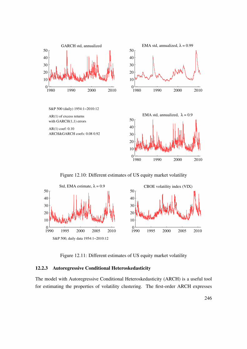
1980 1990 2000 20100
10
20
30
40
50GARCH std, annualized
1980 1990 2000 20100
10
20
30
40
50
EMA std, annualized, λ = 0.99
S&P 500 (daily) 1954:1−2010:12
AR(1) of excess returns
with GARCH(1,1) errors
AR(1) coef: 0.10
ARCH&GARCH coefs: 0.08 0.92
1980 1990 2000 20100
10
20
30
40
50
EMA std, annualized, λ = 0.9
Figure 12.10: Different estimates of US equity market volatility
1990 1995 2000 2005 20100
10
20
30
40
50
Std, EMA estimate, λ = 0.9
S&P 500, daily data 1954:1−2010:12
1990 1995 2000 2005 20100
10
20
30
40
50CBOE volatility index (VIX)
Figure 12.11: Different estimates of US equity market volatility
12.2.3 Autoregressive Conditional Heteroskedasticity
The model with Autoregressive Conditional Heteroskedasticity (ARCH) is a useful toolfor estimating the properties of volatility clustering. The first-order ARCH expresses
246
volatility as a function of the latest squared shock
s2� D ˛0 C ˛1u2��1; (12.15)
where u� is a zero-mean variable. The model requires ˛0 > 0 and 0 � ˛1 < 1 toguarantee that the volatility stays positive and finite. The variance reverts back to anaverage variance (˛0=.1 � ˛1/). The rate of mean reversion is ˛1, that is, the variancebehaves much like an AR(1) model with an autocorrelation parameter of ˛1. The modelparameters are typically estimated by maximum likelihood. Higher-order ARCH modelsinclude further lags of the squared shocks (for instance, u2��2).
Instead of using a high-order ARCH model, it is often convenient to use a first-ordergeneralized ARCH model, the GARCH(1,1) model. It adds a term that captures directautoregression of the volatility
s2� D ˛0 C ˛1u2��1 C ˇ1s2��1: (12.16)
We require that ˛0 > 0, ˛1 � 0, ˇ1 � 0, and ˛1 C ˇ1 < 1 to guarantee that thevolatility stays positive and finite. This is very similar to the EMA in (12.14), except thatthe variance reverts back to the mean (˛0=.1 � ˛1 � ˇ1/). The rate of mean reversion is˛1 C ˇ1, that is, the variance behaves much like an AR(1) model with an autocorrelationparameter of ˛1 C ˇ1.
12.2.4 Time-Variation in Volatility and the B-S Formula
The ARCH and GARCH models imply that volatility is random, so they are (strictlyspeaking) not consistent with the B-S model. However, they are often combined with theB-S model to provide an approximate option price. See Figure 12.12 for a comparison ofthe actual distribution of the log asset price at different horizons (10 and 100 days) whenthe daily returns are generated by a GARCH model—and a normal distribution with thesame mean and variance. To be specific, the figure with a 10-day horizon shows thedistribution of lnStCm, as seen from period t , where lnStCm is calculated as
lnStCm D lnSt C u� C u�C1 C : : :C u�C10; (12.17)
where each of the growth rates (u� ) is drawn from an N.0; s2� ) distribution where thevariance follows the GARCH(1,1) process in (12.16).
247
It is clear the normal distribution is a good approximation unless the horizon is shortand the ARCH component (˛1u2��1) dominates the GARCH component (ˇ1s2��1). Intu-itively, we get (almost) a normal distribution in two cases. First, when the random partof the volatility (˛1u2��1) is relatively small compared to the non-random part (ˇ1s2��1).For instance, if there is no random part at all, then we get exactly a normal distribution(the sum of normally distributed variables is normally distributed—if all the variances aredeterministic). Second, the summing of many uncorrelated growth rates in (12.17) givethe same effect as taking an average: if we average sufficiently many components we geta distribution that looks more and more similar to a normal distribution (this is the centrallimit theorem).
However, to get an option price that is perfectly consistent with a GARCH process,we need to go beyond the B-S model (see, for instance, Heston and Nandi (2000)).
Remark 12.9 (Time-varying, but deterministic volatility�) A time-varying, but non-random
volatility could be consistent with (12.2): if lnStCm is the sum (integral) of normally dis-
tributed changes with known (but time-varying variances), then this sum has a normal
distribution (recall: if the random variables x and y are normally distributed, so is xCy).
A random variance does not fit this case, since a variable with a random variance is not
normally distributed.
Bibliography
Bodie, Z., A. Kane, and A. J. Marcus, 2005, Investments, McGraw-Hill, Boston, 6th edn.
Campbell, J. Y., A. W. Lo, and A. C. MacKinlay, 1997, The econometrics of financial
markets, Princeton University Press, Princeton, New Jersey.
Elton, E. J., M. J. Gruber, S. J. Brown, and W. N. Goetzmann, 2003, Modern portfolio
theory and investment analysis, John Wiley and Sons, 6th edn.
Gourieroux, C., and J. Jasiak, 2001, Financial econometrics: problems, models, and
methods, Princeton University Press.
Heston, S. L., and S. Nandi, 2000, “A closed-form GARCH option valuation model,”Review of Financial Studies, 13, 585–625.
248

−20 −10 0 10 200
0.05
0.1GARCH distribution, T = 10 days
Return
(α β) = (0.8 0.09) N
Sim
−40 −20 0 20 400
0.01
0.02
0.03GARCH distribution, T = 100 days
(α β) = (0.8 0.09)
Return
−15 −10 −5 0 5 10 150
0.05
0.1
0.15GARCH distribution, T = 10 days
(α β) = (0.09 0.8)
Return
−40 −20 0 20 400
0.01
0.02
0.03
0.04GARCH distribution, T = 100 days
(α β) = (0.09 0.8)
Return
Figure 12.12: Comparison of normal and simulated distribution of m-period returns
Hull, J. C., 2006, Options, futures, and other derivatives, Prentice-Hall, Upper SaddleRiver, NJ, 6th edn.
Taylor, S. J., 2005, Asset price dynamics, volatility, and prediction, Princeton UniversityPress.
249
13 Event Studies
Reference: Bodie, Kane, and Marcus (2005) 12.3 or Copeland, Weston, and Shastri(2005) 11Reference (advanced): Campbell, Lo, and MacKinlay (1997) 4More advanced material is denoted by a star (�). It is not required reading.
13.1 Basic Structure of Event Studies
The idea of an event study is to study the effect (on stock prices or returns) of a specialevent by using a cross-section of such events. For instance, what is the effect of a stocksplit announcement on the share price? Other events could be debt issues, mergers andacquisitions, earnings announcements, or monetary policy moves.
The event is typically assumed to be a discrete variable. For instance, it could be amerger or not or if the monetary policy surprise was positive (lower interest than expected)or not. The basic approach is then to study what happens to the returns of those assetsthat have such an event.
Only news should move the asset price, so it is often necessary to explicitly modelthe previous expectations to define the event. For earnings, the event is typically taken tobe the earnings announcement minus (some average of) analysts’ forecast. Similarly, formonetary policy moves, the event could be specified as the interest rate decision minusprevious forward rates (as a measure of previous expectations).
The abnormal return of asset i in period t is
ui;t D Ri;t �Rnormali;t ; (13.1)
where Rit is the actual return and the last term is the normal return (which may differacross assets and time). The definition of the normal return is discussed in detail in Section13.2. These returns could be nominal returns, but more likely (at least for slightly longerhorizons) real returns or excess returns.
Suppose we have a sample of n such events (“assets”). To keep the notation (reason-
250
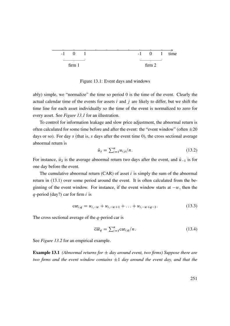
-1 0 1 -1 0 1 time
firm 1 firm 2
Figure 13.1: Event days and windows
ably) simple, we “normalize” the time so period 0 is the time of the event. Clearly theactual calendar time of the events for assets i and j are likely to differ, but we shift thetime line for each asset individually so the time of the event is normalized to zero forevery asset. See Figure 13.1 for an illustration.
To control for information leakage and slow price adjustment, the abnormal return isoften calculated for some time before and after the event: the “event window” (often˙20days or so). For day s (that is, s days after the event time 0), the cross sectional averageabnormal return is
Nus DPniD1ui;s=n: (13.2)
For instance, Nu2 is the average abnormal return two days after the event, and Nu�1 is forone day before the event.
The cumulative abnormal return (CAR) of asset i is simply the sum of the abnormalreturn in (13.1) over some period around the event. It is often calculated from the be-ginning of the event window. For instance, if the event window starts at �w, then theq-period (day?) car for firm i is
cari;q D ui;�w C ui;�wC1 C : : :C ui;�wCq�1: (13.3)
The cross sectional average of the q-period car is
carq DPniD1cari;q=n: (13.4)
See Figure 13.2 for an empirical example.
Example 13.1 (Abnormal returns for ˙ day around event, two firms) Suppose there are
two firms and the event window contains ˙1 day around the event day, and that the
251
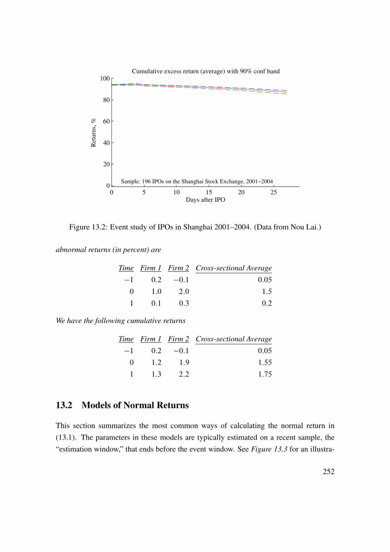
0 5 10 15 20 250
20
40
60
80
100Cumulative excess return (average) with 90% conf band
Days after IPO
Ret
urn
s, %
Sample: 196 IPOs on the Shanghai Stock Exchange, 2001−2004
Figure 13.2: Event study of IPOs in Shanghai 2001–2004. (Data from Nou Lai.)
abnormal returns (in percent) are
Time Firm 1 Firm 2 Cross-sectional Average
�1 0:2 �0:1 0:05
0 1:0 2:0 1:5
1 0:1 0:3 0:2
We have the following cumulative returns
Time Firm 1 Firm 2 Cross-sectional Average
�1 0:2 �0:1 0:05
0 1:2 1:9 1:55
1 1:3 2:2 1:75
13.2 Models of Normal Returns
This section summarizes the most common ways of calculating the normal return in(13.1). The parameters in these models are typically estimated on a recent sample, the“estimation window,” that ends before the event window. See Figure 13.3 for an illustra-
252

tion. (When there is no return data before the event window (for instance, when the eventis an IPO), then the estimation window can be after the event window.)
In this way, the estimated behaviour of the normal return should be unaffected by theevent. It is almost always assumed that the event is exogenous in the sense that it is notdue to the movements in the asset price during either the estimation window or the eventwindow. This allows us to get a clean estimate of the normal return.
The constant mean return model assumes that the return of asset i fluctuates randomlyaround some mean �i
Ri;t D �i C �i;t with E.�i;t/ D Cov.�i;t ; �i;t�s/ D 0: (13.5)
This mean is estimated by the sample average (during the estimation window). The nor-mal return in (13.1) is then the estimated mean. O�i so the abnormal return becomes O�i;t .
The market model is a linear regression of the return of asset i on the market return
Ri;t D ˛iCˇiRm;tC"it with E."i;t/ D Cov."i;t ; "i;t�s/ D Cov."i;t ; Rm;t/ D 0: (13.6)
Notice that we typically do not impose the CAPM restrictions on the intercept in (13.6).The normal return in (13.1) is then calculated by combining the regression coefficientswith the actual market return as O i C OiRm;t , so the the abnormal return becomes O"it .
When we restrict ˛i D 0 and ˇi D 1, then this approach is called the market-adjusted-
return model. This is a particularly useful approach when there is no return data beforethe event, for instance, with an IPO.
Recently, the market model has increasingly been replaced by a multi-factor modelwhich uses several regressors instead of only the market return. For instance, Fama andFrench (1993) argue that (13.6) needs to be augmented by a portfolio that captures thedifferent returns of small and large firms and also by a portfolio that captures the differentreturns of firms with high and low book-to-market ratios.
Finally, another approach is to construct a normal return as the actual return on assetswhich are very similar to the asset with an event. For instance, if asset i is a small man-ufacturing firm (with an event), then the normal return could be calculated as the actualreturn for other small manufacturing firms (without events). In this case, the abnormalreturn becomes the difference between the actual return and the return on the matchingportfolio. This type of matching portfolio is becoming increasingly popular.
253

time
estimation window(for normal return)
event window
Figure 13.3: Event and estimation windows
All the methods discussed here try to take into account the risk premium on the asset.It is captured by the mean in the constant mean mode, the beta in the market model, andby the way the matching portfolio is constructed. However, sometimes there is no data inthe estimation window. The typical approach is then to use the actual market return as thenormal return—that is, to use (13.6) but assuming that ˛i D 0 and ˇi D 1. Clearly, thisdoes not account for the risk premium on asset i , and is therefore a fairly rough guide.
Apart from accounting for the risk premium, does the choice of the model of thenormal return matter a lot? Yes, but only if the model produces a higher coefficient ofdetermination (R2) than competing models. In that case, the variance of the abnormalreturn is smaller for the market model which the test more precise (see Section 13.3 fora discussion of how the variance of the abnormal return affects the variance of the teststatistic). To illustrate this, consider the market model (13.6). Under the null hypothesisthat the event has no effect on the return, the abnormal return would be just the residualin the regression (13.6). It has the variance (assuming we know the model parameters)
Var.ui;t/ D Var."it/ D .1 �R2/Var.Ri;t/; (13.7)
where R2 is the coefficient of determination of the regression (13.6).Proof. (of (13.7)) From (13.6) we have
Var.Ri;t/ D ˇ2i Var.Rm;t/C Var."it/:
254
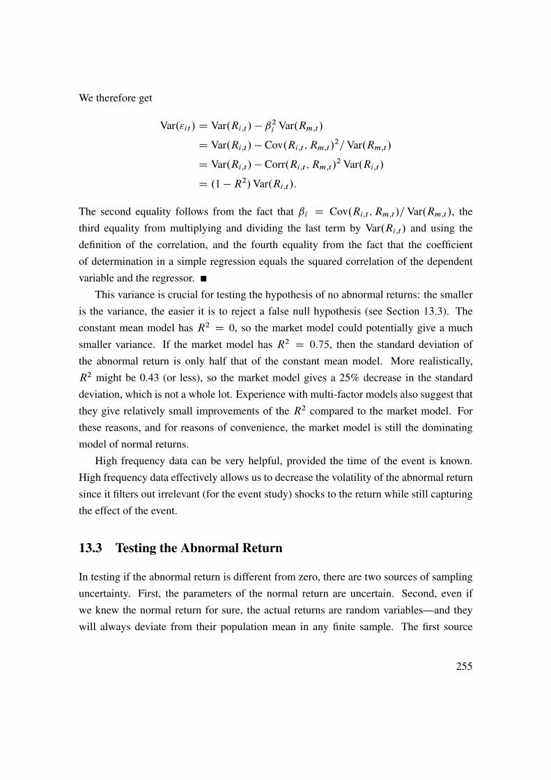
We therefore get
Var."it/ D Var.Ri;t/ � ˇ2i Var.Rm;t/
D Var.Ri;t/ � Cov.Ri;t ; Rm;t/2=Var.Rm;t/
D Var.Ri;t/ � Corr.Ri;t ; Rm;t/2 Var.Ri;t/
D .1 �R2/Var.Ri;t/:
The second equality follows from the fact that ˇi D Cov.Ri;t ; Rm;t/=Var.Rm;t/, thethird equality from multiplying and dividing the last term by Var.Ri;t/ and using thedefinition of the correlation, and the fourth equality from the fact that the coefficientof determination in a simple regression equals the squared correlation of the dependentvariable and the regressor.
This variance is crucial for testing the hypothesis of no abnormal returns: the smalleris the variance, the easier it is to reject a false null hypothesis (see Section 13.3). Theconstant mean model has R2 D 0, so the market model could potentially give a muchsmaller variance. If the market model has R2 D 0:75, then the standard deviation ofthe abnormal return is only half that of the constant mean model. More realistically,R2 might be 0.43 (or less), so the market model gives a 25% decrease in the standarddeviation, which is not a whole lot. Experience with multi-factor models also suggest thatthey give relatively small improvements of the R2 compared to the market model. Forthese reasons, and for reasons of convenience, the market model is still the dominatingmodel of normal returns.
High frequency data can be very helpful, provided the time of the event is known.High frequency data effectively allows us to decrease the volatility of the abnormal returnsince it filters out irrelevant (for the event study) shocks to the return while still capturingthe effect of the event.
13.3 Testing the Abnormal Return
In testing if the abnormal return is different from zero, there are two sources of samplinguncertainty. First, the parameters of the normal return are uncertain. Second, even ifwe knew the normal return for sure, the actual returns are random variables—and theywill always deviate from their population mean in any finite sample. The first source
255

of uncertainty is likely to be much smaller than the second—provided the estimationwindow is much longer than the event window. This is the typical situation, so the rest ofthe discussion will focus on the second source of uncertainty.
It is typically assumed that the abnormal returns are uncorrelated across time andacross assets. The first assumption is motivated by the very low autocorrelation of returns.The second assumption makes a lot of sense if the events are not overlapping in time, sothat the event of assets i and j happen at different (calendar) times. It can also be arguedthat the model for the normal return (for instance, a market model) should capture allcommon movements by the regressors — leaving the abnormal returns (the residuals)uncorrelated across firms. In contrast, if the events happen at the same time, the cross-correlation must be handled somehow. This is, for instance, the case if the events aremacroeconomic announcements or monetary policy moves. An easy way to handle suchsynchronized (clustered) events is to form portfolios of those assets that share the eventtime—and then only use portfolios with non-overlapping events in the cross-sectionalstudy. For the rest of this section we assume no autocorrelation or cross correlation.
Let �2i D Var.ui;t/ be the variance of the abnormal return of asset i . The variance ofthe cross-sectional (across the n assets) average, Nus in (13.2), is then
Var. Nus/ D��21 C �22 C :::C �2n
�=n2 DPn
iD1�2i =n
2; (13.8)
since all covariances are assumed to be zero. In a large sample (where the asymptoticnormality of a sample average starts to kick in), we can therefore use a t -test since
Nus=Std. Nus/!d N.0; 1/: (13.9)
The cumulative abnormal return over q period, cari;q, can also be tested with a t -test.Since the returns are assumed to have no autocorrelation the variance of the cari;q
Var.cari;q/ D q�2i : (13.10)
This variance is increasing in q since we are considering cumulative returns (not the timeaverage of returns).
The cross-sectional average cari;q is then (similarly to (13.8))
Var.carq/ D�q�21 C q�22 C :::C q�2n
�=n2 D qPn
iD1�2i =n
2; (13.11)
256

if the abnormal returns are uncorrelated across time and assets.Figures 4.2a–b in Campbell, Lo, and MacKinlay (1997) provide a nice example of an
event study (based on the effect of earnings announcements).
Example 13.2 (Variances of abnormal returns) If the standard deviations of the daily
abnormal returns of the two firms in Example 13.1 are �1 D 0:1 and and �2 D 0:2, then
we have the following variances for the abnormal returns at different days
Time Firm 1 Firm 2 Cross-sectional Average
�1 0:12 0:22�0:12 C 0:22� =4
0 0:12 0:22�0:12 C 0:22� =4
1 0:12 0:22�0:12 C 0:22� =4
Similarly, the variances for the cumulative abnormal returns are
Time Firm 1 Firm 2 Cross-sectional Average
�1 0:12 0:22�0:12 C 0:22� =4
0 2 � 0:12 2 � 0:22 2 � �0:12 C 0:22� =41 3 � 0:12 3 � 0:22 3 � �0:12 C 0:22� =4
Example 13.3 (Tests of abnormal returns) By dividing the numbers in Example 13.1 by
the square root of the numbers in Example 13.2 (that is, the standard deviations) we get
the test statistics for the abnormal returns
Time Firm 1 Firm 2 Cross-sectional Average
�1 2 �0:5 0:4
0 10 10 13:4
1 1 1:5 1:8
Similarly, the variances for the cumulative abnormal returns we have
Time Firm 1 Firm 2 Cross-sectional Average
�1 2 �0:5 0:4
0 8:5 6:7 9:8
1 7:5 6:4 9:0
257

13.4 Quantitative Events
Some events are not easily classified as discrete variables. For instance, the effect ofpositive earnings surprise is likely to depend on how large the surprise is—not just if therewas a positive surprise. This can be studied by regressing the abnormal return (typicallythe cumulative abnormal return) on the value of the event (xi )
cari;q D aC bxi C �i : (13.12)
The slope coefficient is then a measure of how much the cumulative abnormal returnreacts to a change of one unit of xi .
Bibliography
Bodie, Z., A. Kane, and A. J. Marcus, 2005, Investments, McGraw-Hill, Boston, 6th edn.
Campbell, J. Y., A. W. Lo, and A. C. MacKinlay, 1997, The econometrics of financial
markets, Princeton University Press, Princeton, New Jersey.
Copeland, T. E., J. F. Weston, and K. Shastri, 2005, Financial theory and corporate policy,Pearson Education, 4 edn.
Fama, E. F., and K. R. French, 1993, “Common risk factors in the returns on stocks andbonds,” Journal of Financial Economics, 33, 3–56.
258

14 Kernel Density Estimation and Regression
14.1 Non-Parametric Regression
Reference: Campbell, Lo, and MacKinlay (1997) 12.3; Härdle (1990); Pagan and Ullah(1999); Mittelhammer, Judge, and Miller (2000) 21
14.1.1 Simple Kernel Regression
Non-parametric regressions are used when we are unwilling to impose a parametric formon the regression equation—and we have a lot of data.
Let the scalars yt and xt be related as
yt D b.xt/C "t ; "t is iid and E "t D Cov Œb.xt/; "t � D 0; (14.1)
where b./ is a, possibly non-linear, function.Suppose the sample had 3 observations (say, t D 3, 27, and 99) with exactly the same
value of xt , say 1:9. A natural way of estimating b.x/ at x D 1:9 would then be toaverage over these 3 observations as we can expect average of the error terms to be closeto zero (iid and zero mean).
Unfortunately, we seldom have repeated observations of this type. Instead, we maytry to approximate the value of b.x/ (x is a single value, 1.9, say) by averaging overobservations where xt is close to x. The general form of this type of estimator is
Ob.x/ D w.x1 � x/y1 C w.x2 � x/y2 C : : :C w.xT � x/yTw.x1 � x/C w.x2 � x/C : : :C w.xT � x/
DPT
tD1w.xt � x/ytPTtD1w.xt � x/
; (14.2)
where w.xt � x/=˙TtD1w.xt � x/ is the weight given to observation t . The function
w.xi � x/ is a positive and (weakly) increasing in the distance between xi and x. Notethat denominator makes the weights sum to unity. The basic assumption behind (14.2) isthat the b.x/ function is smooth so local (around x) averaging makes sense.
259

As an example of a w.:/ function, it could give equal weight to the k values of xtwhich are closest to x and zero weight to all other observations (this is the “k-nearestneighbor” estimator, see Härdle (1990) 3.2). As another example, the weight functioncould be defined so that it trades off the expected squared errors, EŒyt � Ob.x/�2, and theexpected squared acceleration, EŒd 2 Ob.x/=dx2�2. This defines a cubic spline (and is oftenused in macroeconomics, where xt D t and is then called the Hodrick-Prescott filter).
A Kernel regression uses a pdf as the weight function w.:/. The pdf of N.0; h2/is commonly used, where the choice of h allows us to easily vary the relative weightsof different observations. This weighting function is positive so all observations get apositive weight, but the weights are highest for observations close to x and then tapers ofin a bell-shaped way. See Figure 14.1 for an illustration.
A low value of h means that the weights taper off fast—the weight function is then anormal pdf with a low variance. With this particular kernel, we get the following estimatorof b.x/ at a point x
Ob.x/ DPT
tD1Kh.xt � x/ytPTtD1Kh.xt � x/
, where Kh.xt � x/ D expŒ�.xt � x/2=.2h2/�hp2�
: (14.3)
Note that Kh.xt � x/ corresponds to the weighting function w.xt � x/ in (14.2).In practice we have to estimate Ob.x/ at a finite number of points x. This could, for
instance, be 100 evenly spread points in the interval between the minimum and maximumvalues observed in the sample. See Figure 14.2 for an illustration. Special correctionsmight be needed if there are a lot of observations stacked close to the boundary of thesupport of x (see Härdle (1990) 4.4).
A good (but computationally intensive) approach to choose h is by the leave-one-outcross-validation technique. This approach would, for instance, choose h to minimize theexpected (or average) prediction error
EPE.h/ DXT
tD1
hyt � Ob�t.xt ; h/
i2=T; (14.4)
where Ob�t.xt ; h/ is the fitted value at xt when we use a regression function estimated ona sample that excludes observation t , and a bandwidth h. This means that each predictionis out-of-sample. To calculate (14.4) we clearly need to make T estimations (for eachxt )—and then repeat this for different values of h to find the minimum.
260

1.4 1.6 1.8 2 2.2 2.4
4
5
Data and weights for b(1.7)
xt
weights⊗
1.4 1.6 1.8 2 2.2 2.40
1
1.4 1.6 1.8 2 2.2 2.4
4
5
Data and weights for b(1.9)
xt
⊗
1.4 1.6 1.8 2 2.2 2.40
1
1.4 1.6 1.8 2 2.2 2.4
4
5
Data and weights for b(2.1)
xt
⊗
1.4 1.6 1.8 2 2.2 2.40
1
Data on x: 1.5 2.0 2.5
Data on y: 5.0 4.0 3.5
N(0,0.252) kernel
ο denotes the data
⊗ denotes the fitted b(x)
Left y−axis: data; right y−axis: weights
Figure 14.1: Example of kernel regression with three data points
If the observations are independent, then it can be shown (see Härdle (1990) 4.2 andPagan and Ullah (1999) 3.3–6) that, with a Gaussian kernel, the estimator at point x isasymptotically normally distributed
pT h
h Ob.x/ � E Ob.x/i!d N
�0;
1
2p�
�2.x/
f .x/
�; (14.5)
where �2.x/ is the variance of the residuals in (14.1) and f .x/ the marginal density of x.To estimate the density function neeeded in (14.5), we can use a kernel density esti-
mator of the pdf at some point x
Of .x/ D 1
T h
XT
tD1K�xt � x
h
�, where K.u/ D exp
��u2=2�p2�
: (14.6)
The value h D Std.xt/1:06T �1=5 is sometimes recommended, since it can be shown to be
261

1.4 1.6 1.8 2 2.2 2.4 2.6
3.5
4
4.5
5
Kernel regression
x
y
Data
h= 0.25
h= 0.2
Figure 14.2: Example of kernel regression with three data points
the optimal choice (in MSE sense) if data is normally distributed and the N.0; 1/ kernelis used. Clearly, using K Œ.xt � x/=h� =h is the same as using pdf of N.x; h2/.
To estimate �2.x/ also needed in (14.5), a non-parametric regression ofhyt � Ob�t.xt/
i2on xt can be used.
Example 14.1 Suppose the sample has three data points Œx1; x2; x3� D Œ1:5; 2; 2:5� and
Œy1; y2; y3� D Œ5; 4; 3:5�. Consider the estimation of b.x/ at x D 1:9. With h D 1, the
numerator in (14.3) isXT
tD1Kh.xt � x/yt D
�e�.1:5�1:9/
2=2 � 5C e�.2�1:9/2=2 � 4C e�.2:5�1:9/2=2 � 3:5�=p2�
� .0:92 � 5C 1:0 � 4C 0:84 � 3:5/ =p2�
D 11:52=p2�:
The denominator isXT
tD1Kh.xt � x/ D
�e�.1:5�1:9/
2=2 C e�.2�1:9/2=2 C e�.2:5�1:9/2=2�=p2�
� 2:75=p2�:
262

0 5 10 15 20−0.2
−0.1
0
0.1Drift vs level, in bins
yt
∆y
t+1
Daily federal funds rates 1954:7−2010:9
0 5 10 15 200
0.5
1
1.5Volatility vs level, in bins
yt
Vol t+
1 V olt+1 = (∆yt+1 − ∆yt+1 )2
Figure 14.3: Federal funds rate, crude non-parametric regression
0 5 10 15 20−0.2
−0.1
0
0.1Drift vs level, kernel regression
yt
∆y t+
1
Daily federal funds rates 1954:7−2010:9
Small h
Large h
0 5 10 15 200
0.5
1
1.5Vol vs level, kernel regression
yt
Vol t+
1
V olt+1 = (∆yt+1 − ∆yt+1 )2
Small h
Large h
Figure 14.4: Federal funds rate, non-parametric regression
The estimate at x D 1:9 is therefore
Ob.1:9/ � 11:52=2:75 � 4:19:
Kernel regressions are typically consistent, provided longer samples are accompaniedby smaller values of h, so the weighting function becomes more and more local as thesample size increases.
See Figures 14.3–14.4 for an example. Note that the volatility is defined as the squareof the drift minus expected drift (from the same estimation method).
263
0 5 10 15 20−0.2
−0.1
0
0.1Drift vs level, kernel regression
yt
∆y
t+1
Daily federal funds rates 1954:7−2010:9
Point estimate and90% confidence band
0 5 10 15 200
0.5
1
1.5Vol vs level, kernel regression
yt
Vol t+
1
V olt+1 = (∆yt+1 − ∆yt+1 )2
Figure 14.5: Federal funds rate, non-parametric regression with confidence bands
14.1.2 Multivariate Kernel Regression
Suppose that yt depends on two variables (xt and zt )
yt D b.xt ; zt/C "t ; "t is iid and E "t D 0: (14.7)
This makes the estimation problem much harder since there are typically few observationsin every bivariate bin (rectangle) of x and z. For instance, with as little as a 20 intervals ofeach of x and z, we get 400 bins, so we need a large sample to have a reasonable numberof observations in every bin.
In any case, the most common way to implement the kernel regressor is to let
Ob.x; z/ DPT
tD1Khx.xt � x/Khz.zt � z/ytPTtD1Khx.xt � x/Khz.zt � z/
; (14.8)
where Khx.xt � x/ and Khz.zt � z/ are two kernels like in (14.3) and where we mayallow hx and hy to be different (and depend on the variance of xt and yt ). In this case.the weight of the observation (xt ; zt ) is proportional to Khx.xt � x/Khz.zt � z/, whichis high if both xt and yt are close to x and y respectively.
See Figure 14.4 for an example.
264

14.2 Examples of Non-Parametric Estimation
14.2.1 A Model for the Short Interest Rate
Interest rate models are typically designed to describe the movements of the entire yieldcurve in terms of a small number of factors. For instance, the model assumes that theshort interest rate, rt , is a mean-reverting AR(1) process
rt D �rt�1 C "t ; where "t � N.0; �2/, so (14.9)
rt � rt�1 D .� � 1/rt�1 C "t ; (14.10)
and that all term premia are constant. This means that the drift is decreasing in the interestrate, but that the volatility is constant.
(The usual assumption is that the short interest rate follows an Ornstein-Uhlenbeckdiffusion process, which implies the discrete time model in (14.9).) It can then be shownthat all interest rates (for different maturities) are linear functions of short interest rates.
To capture more movements in the yield curve, models with richer dynamics are used.For instance, Cox, Ingersoll, and Ross (1985) construct a model which implies that theshort interest rate follows an AR(1) as in (14.9) except that the variance is proportional tothe interest rate level, so "t � N.0; rt�1�2/.
Recently, non-parametric methods have been used to estimate how the drift and volatil-ity are related to the interest rate level (see, for instance, Ait-Sahalia (1996)). Figures14.3–14.4 give an example. Note that the volatility is defined as the square of the driftminus expected drift (from the same estimation method).
14.2.2 Non-Parametric Option Pricing
There seems to be systematic deviations from the Black-Scholes model. For instance,implied volatilities are often higher for options far from the current spot (or forward)price—the volatility smile. This is sometimes interpreted as if the beliefs about the futurelog asset price put larger probabilities on very large movements than what is compatiblewith the normal distribution (“fat tails”).
This has spurred many efforts to both describe the distribution of the underlying assetprice and to amend the Black-Scholes formula by adding various adjustment terms. Onestrand of this literature uses non-parametric regressions to fit observed option prices to
265

the variables that also show up in the Black-Scholes formula (spot price of underlyingasset, strike price, time to expiry, interest rate, and dividends). For instance, Ait-Sahaliaand Lo (1998) applies this to daily data for Jan 1993 to Dec 1993 on S&P 500 indexoptions (14,000 observations). They find interesting patterns of the implied moments(mean, volatility, skewness, and kurtosis) as the time to expiry changes. In particular, thenon-parametric estimates suggest that distributions for longer horizons have increasinglylarger skewness and kurtosis. Whereas the distributions for short horizons are not toodifferent from normal distributions, this is not true for longer horizons.
Bibliography
Ait-Sahalia, Y., 1996, “Testing Continuous-Time Models of the Spot Interest Rate,” Re-
view of Financial Studies, 9, 385–426.
Ait-Sahalia, Y., and A. W. Lo, 1998, “Nonparametric Estimation of State-Price DensitiesImplicit in Financial Asset Prices,” Journal of Finance, 53, 499–547.
Campbell, J. Y., A. W. Lo, and A. C. MacKinlay, 1997, The Econometrics of Financial
Markets, Princeton University Press, Princeton, New Jersey.
Cox, J. C., J. E. Ingersoll, and S. A. Ross, 1985, “A Theory of the Term Structure ofInterest Rates,” Econometrica, 53, 385–407.
Härdle, W., 1990, Applied Nonparametric Regression, Cambridge University Press, Cam-bridge.
Mittelhammer, R. C., G. J. Judge, and D. J. Miller, 2000, Econometric Foundations, Cam-bridge University Press, Cambridge.
Pagan, A., and A. Ullah, 1999, Nonparametric Econometrics, Cambridge UniversityPress.
266