
Lecture Notes Geometric Measure Theory
162
Lecture Notes Geometric Measure Theory Course held by Notes written by Prof. Giovanni Alberti Francesco Paolo Maiale Department of Mathematics Pisa University December 27, 2017
Transcript of Lecture Notes Geometric Measure Theory

Lecture Notes
Geometric Measure Theory
Course held by Notes written by
Prof. Giovanni Alberti Francesco Paolo Maiale
Department of Mathematics
Pisa University
December 27, 2017

Disclaimer
These notes came out of the Geometric Measure Theory course, held by Professor Gio-
vanni Alberti in the second semester of the academic year 2016/2017.
They include all the topics that were discussed in class; I added some remarks, simple
proof, etc.. for my convenience.
I have used them to study for the exam; hence they have been reviewed thoroughly.
Unfortunately, there may still be many mistakes and oversights; to report them, send me
an email at francescopaolo (dot) maiale (at) gmail (dot) com.

Contents
I Introduction to Measure Theory 5
1 Introduction 6
1.1 Plateau’s Problem . . . . . . . . . . . . . . . . . . . . . . . . . . . . . . . . . 6
1.2 Geodesics problem (d = 1) . . . . . . . . . . . . . . . . . . . . . . . . . . . . . 7
1.3 ”Surface” Problem (d > 1) . . . . . . . . . . . . . . . . . . . . . . . . . . . . . 8
2 Measure Theory 9
2.1 Definitions and Elementary Properties . . . . . . . . . . . . . . . . . . . . . . 9
2.2 Weak-∗ Topology on Measures Space . . . . . . . . . . . . . . . . . . . . . . . 12
2.3 Outer Measures . . . . . . . . . . . . . . . . . . . . . . . . . . . . . . . . . . . 17
2.4 Caratheodory Construction . . . . . . . . . . . . . . . . . . . . . . . . . . . . 21
2.5 Hausdorff d-dimensional Measure Hd . . . . . . . . . . . . . . . . . . . . . . . 23
2.6 Hausdorff Dimension of Cantor-Type Sets . . . . . . . . . . . . . . . . . . . . 31
II Covering Results 34
3 Covering Theorem 35
3.1 Vitali Covering Theorem . . . . . . . . . . . . . . . . . . . . . . . . . . . . . . 36
3.2 Besicovitch Covering Theorem . . . . . . . . . . . . . . . . . . . . . . . . . . 41
III Geometric Measure Theory 45
4 Density of Measures 46
4.1 Density of Doubling Locally Finite Measures . . . . . . . . . . . . . . . . . . 46
4.2 Upper Density of the Hausdorff Measure . . . . . . . . . . . . . . . . . . . . . 47
4.3 Upper d-Dimensional Density . . . . . . . . . . . . . . . . . . . . . . . . . . . 52
4.4 Applications . . . . . . . . . . . . . . . . . . . . . . . . . . . . . . . . . . . . . 60
5 Self-Similar Sets 63

IV Rectifiability 71
6 Other measures and dimensions 72
6.1 Geometric Integral Measure . . . . . . . . . . . . . . . . . . . . . . . . . . . . 72
6.2 Invariant Measures on Topological Groups . . . . . . . . . . . . . . . . . . . . 74
7 Lipschitz Functions 78
7.1 Definitions and Main Properties . . . . . . . . . . . . . . . . . . . . . . . . . . 78
7.2 Differentiability of Lipschitz Functions . . . . . . . . . . . . . . . . . . . . . . 79
7.3 Area Formula for Lipschitz Maps . . . . . . . . . . . . . . . . . . . . . . . . . 83
7.4 Coarea Formula for Lipschitz Maps . . . . . . . . . . . . . . . . . . . . . . . . 87
8 Rectifiable Sets 89
8.1 Introduction and Elementary Properties . . . . . . . . . . . . . . . . . . . . . 89
8.2 Tangent Bundle . . . . . . . . . . . . . . . . . . . . . . . . . . . . . . . . . . . 95
8.3 Rectifiability Criteria . . . . . . . . . . . . . . . . . . . . . . . . . . . . . . . . 101
8.4 Area Formula for Rectifiable Sets . . . . . . . . . . . . . . . . . . . . . . . . . 106
V Finite Perimeter Sets 108
9 Bounded Variation Functions 109
9.1 Definition and Elementary Properties . . . . . . . . . . . . . . . . . . . . . . 109
9.2 Alternative Definitions: Bounded Variation on the Real Line . . . . . . . . . 112
9.3 Functional Properties . . . . . . . . . . . . . . . . . . . . . . . . . . . . . . . 114
10 Finite Perimeter Sets 121
10.1 Main Definitions and Elementary Properties . . . . . . . . . . . . . . . . . . . 121
10.2 Approximation Theorem via Coarea Formula . . . . . . . . . . . . . . . . . . 123
10.3 Existence Results for Plateau’s Problem . . . . . . . . . . . . . . . . . . . . . 125
10.4 Capillarity Problem . . . . . . . . . . . . . . . . . . . . . . . . . . . . . . . . 128
10.5 Finite Perimeter Sets: Structure Theorem . . . . . . . . . . . . . . . . . . . . 132
10.6 Back to the Capillarity Problem . . . . . . . . . . . . . . . . . . . . . . . . . 146
11 Appendix 149
11.1 First Variation of a Functional . . . . . . . . . . . . . . . . . . . . . . . . . . 149
11.2 Regularity in Capillarity Problems . . . . . . . . . . . . . . . . . . . . . . . . 154
11.3 Regularity in the F.P.S. Setting . . . . . . . . . . . . . . . . . . . . . . . . . . 155
11.4 Structure of Finite Length Continua in Rn . . . . . . . . . . . . . . . . . . . . 157
11.5 Lower Semi-Continuity: Golab Theorem . . . . . . . . . . . . . . . . . . . . . 159
11.6 Simons’ Cone . . . . . . . . . . . . . . . . . . . . . . . . . . . . . . . . . . . . 159

Part I
Introduction to Measure Theory
5

Chapter 1
Introduction
In this chapter, we introduce the main topics of the course and give a brief overview of whatwe will see and what we will be able to prove by the end of the course.
1.1 Plateau’s Problem
The primary goal and the motivating example of this course is the Plateau’s problem,that is, the problem to find the d-dimensional surface Σ of the minimal area with prescribed(d− 1)-dimensional boundary Γ.
By the end, we will be able to prove that a solution indeed exists, but we will not findit explicitly since it is a NP (hard) numerical problem.
As of now, the problem is not well defined. In fact, the notions of surface, area, andboundary make sense in the smooth setting but, as the examples below show, we need towork in a less regular setting.
More precisely, requiring the surface to be smooth is not enough for modeling reasons(e.g., dip a wire frame into a soap solution, form a soap film, and look for the minimalsurface whose boundary is the wire frame), and also for existence reasons.
Example 1.1. Here we give a list of Plateau’s problems with prescribed boundary condi-tions, and we write down the correct solutions, without proving anything.
(a) Let us identify R4 ∼= C× C and, if d = 2, let us consider the smooth boundary givenby
Γ1 :=(S1 × 0
)∪(0 × S1
).
Surprisingly, every minimizing sequence of smooth surfaces converges to a surfacewhich is not smooth at all. Indeed, the solution of the problem is
Σ1 :=(D2 × 0
)∪(0 ×D2
).
The surface Σ1 is clearly singular at the origin, but the singularity may be removed(by factorizing it into two nonsingular surfaces).

7 1.2. GEODESICS PROBLEM (D = 1)
(b) Let us identify R4 ∼= C× C and, if d = 2, let us consider the smooth boundary givenby
Γ2 :=
(z2, z3) : z ∈ S1.
The solution to the Plateau’s problem is
Σ2 :=
(z2, z3) : z ∈ D2,
which is a non-smooth surface, whose singularity cannot be removed (since the poly-nomial z3
1 = z22 cannot be factorized).
(c) Let us identify R8 ∼= R4×R4 and, if d = 7, let us consider the smooth boundary givenby
Γ3 := S3 × S3.
The minimal surface of prescribed boundary Γ3 is
Σ3 :=
(x1, x2) ∈ R4 × R4 : |x1| = |x2| ≤ 1.
To conclude this introductive chapter, we give a brief overview of the main approaches(studied in this course) to the Plateau’s problem, as d ranges between 1 and ∞.
1.2 Geodesics problem (d = 1)
The geodesics problem (that is, find the shortest curve connecting two points) is, surprisingly,still an open in the non-Riemannian setting. However, in the Riemannian setting, thegeodesics problem is completely solved.
Indeed, if we consider the curves parametrized by paths, the length is a well-definednotion, and the associated functional is lower semi-continuous and coercive; hence the com-pactness is easy to prove.
There are many possible approaches to the geodesics problem, e.g., the Steiner approachand the set theoretical approach, which we describe briefly in the remainder of the section.
Steiner Problem. It is also called networks approach, and it is used to prove the existenceof the geodesics and find the explicit expression for it. The reader may consult [1] for adetailed dissertation on the topic.
Set Theoretical Approach. The main idea is to find a closed and connected set Σ ofminimum length, containing a given finite set Γ. As we shall see later in the course, in thiscase the length is a well defined concept: the Hausdorff distance.
In fact, if X is a suitable space (metric, endowed with Hausdorff distance, etc...), thenthe class defined by
X := K ⊆ X : K compact and connected
is compact and, by Gotab theorem1, H1 is lower semi-continuous on X.
1[4] Let C be an infinite collection of non-empty compact sets all lying in a bounded portion B of Rn.Then there exists a sequence Ej of distinct sets of C convergent in the Hausdorff metric to a non-emptycompact set E.
8 1.3. ”SURFACE” PROBLEM (D > 1)
1.3 ”Surface” Problem (d > 1)
3. The Plateau’s problem is much harder when d = 2, but there are still many approachespossible some of which relying, in a certain sense, on the work already done in the geodesicscase.
Set Theoretical Approach. This approach is highly nontrivial. For example, one mayask what does it mean that a compact set Σ spans a boundary Γ? Moreover, there is anotherproblem one should deal with: the 2-dimensional Hausdorff measure H2 is, generally, notlower semi-continuous. The reader may consult [9] for a complete treatise of the topic.
Remark 1.1. Suppose that d = 2, n = 3 and that Σ is a surface with boundary Γ. If γ isanother closed curve, linked to Γ (by a nonzero linking number), then γ ∩ Σ 6= ∅.
Parametric Approach. This method is essentially due to Douglas [3]. The main ideais the following: since a parametrization φ : D2 → Rn defines surfaces in Rn, the areafunctional is well-defined and given by the formula
A(φ) :=
∫D2
∣∣∣∣ ∂ φ∂ s1∧ ∂ φ
∂ s2
∣∣∣∣ ds1 ds2.
On the other hand, the existence through lower semi-continuity and the compactness are adelicate matter, since coercivity is not an easy property to obtain (the integrand is similarto a determinant).
There is a trick which is similar to the one we can use to find geodesics in the differentialgeometry setting. More precisely, we consider the functional
E(φ) :=1
2
∫D2
|∇φ|2 ds1 ds2.
If we find a minimal point φ for E, then φ will be a conformal parametrized minimumfor A. This trick, on the other hand, heavily depends on a nontrivial theorem: every suchΣ admits a conformal re-parametrization.
The lack of conformal parametrization, though, is what stop us from extending the sametrick to dimension d strictly bigger than 2.
Higher Dimension. If the codimension of Σ is equal to 1 (that is, n = d+ 1), then finiteperimeter sets generalize the notion of open (d+ 1)-dimensional sets with smooth boundaryin Rn.
The class of finite perimeter sets has excellent compactness properties and a notion ofarea lower semi-continuous.
This approach is called ”weak” surfaces approach, and it is essentially due to Caccioppoli[2] and De Giorgi [7]. A different approach, working for any d and n, referred to as integralcurrents, was introduced by Federer and Flaming in their joint paper [6].

Chapter 2
Measure Theory
In this chapter, the chief goal is to give a brief introduction to the theory of measure andacquire the fundamental notions needed for the remainder of the course. The reader withan adequate background, may immediately jump to the next section, and use this one as areference.
In the first part, we introduce the only three classes of measures we shall be concernedabout in this course, and then we study the weak-∗ topology and some of the fundamentalproperties of the weak-∗ convergence.
In the second part, we introduce the notion of outer measure, and we show how it canbe used to construct a measure that belongs to one of the classes mentioned above.
In the final part, we construct the Hausdorff d-dimensional measure, denoted by Hd, andwe prove some of the main properties (e.g., the relation with Lipschitz functions). The lastsection is devoted to the computation of the Hausdorff dimension of a Cantor-type set.
2.1 Definitions and Elementary Properties
Introduction. In this course, we will essentially be only concerned with measures thatbelong to one of the following classes:
(1) Positive, σ-additive measures, defined on the Borel σ-algebra of a reasonable space X,e.g. we might assume X metric, locally compact and separable.1
(2) Positive, σ-subadditive measures, defined on the set of all parts P (X). These aregenerally called outer measures.
(3) Real-valued and vector-valued (bounded) σ-additive measures, defined on the Borelσ-algebra.
Remark 2.1. The Borel σ-algebra B(X) is not closed under the action of continuous maps.
1We are not very specific here since the reader may try, whenever possible, to derive, as an exercise, theminimal assumption on X for an assertion to be true.

10 2.1. DEFINITIONS AND ELEMENTARY PROPERTIES
Proof. Let X = [0, 1] ⊂ R, and let us consider a space-filling curve g : [0, 1] −→ [0, 1]2 andthe projection π : [0, 1]2 −→ [0, 1]; the reader may easily check that the map f := π g :[0, 1] −→ [0, 1] is a continuous function.
Thus, given a Borel set S ⊂ [0, 1]2 with π (S) not Borel, it is easy to prove that theimage of the Borel set g−1(S) under f is not Borel.
In this course, we will often introduce a suitable2 outer measure defined on X and, bytaking the restriction to the Borel σ-algebra (see Theorem 2.14), we automatically obtain ameasure which belongs to the class (1).
Remark 2.2. If X is a separable Banach space3, then the class of measures (3) is thedual space of a particular subspace of C0(X). In the next section, we will also prove that,if the space of measures is endowed with the weak-∗ topology, then this class has goodcompactness properties (that is, the Banach-Alaoglu theorem holds true).
Definition 2.1 (Vector-valued Measure). Let B(X) be a Borel σ-algebra on X, and let Fbe a normed space. A function µ : X −→ F is a σ-additive F -valued measure if
∑n∈N
µ (En) = µ
(⋃n∈N
En
), (2.1)
for any countable disjoint family of Borel sets Enn∈N ⊂ B(X).
Remark 2.3. The identity (2.1) does not only imply the σ-additivity of the measure, butit also gives us a stronger property.
More precisely, the sum on the left-hand side does not depend on the order of the indexes,and thus, if F is a finite-dimensional space, then it is enough to infer that the sum convergesabsolutely.
Representation Theorem. In this final brief paragraph, we sketch the proof of the Rieszrepresentation theorem, according to which the class of measures (3) is the dual of a suitablesubset of the space of all continuous functions.
Definition 2.2 (Total Variation). Let µ be a measure. The total variation of a set E ⊆ Xis the supremum of the measure over the possible countable partitions, that is,
|µ| (E) := sup
+∞∑n=0
|µ(En)|
∣∣∣∣∣ Enn∈N countable partition of E
. (2.2)
Clearly, the total variation is a positive bounded measure, defined on the Borel σ-algebraB(X). The mass of µ is defined by setting
‖µ‖ := |µ| (X). (2.3)
The formula (2.3) defines a norm on the space of all the F -valued σ-Borel measures, whichis also complete. Moreover, it is easy to see that µ is absolutely continuous with respect
2See Section 2.4 for a more precise definition of what suitable means here.
3It is not necessary to require X to be a separable Banach space, but it is more than enough for ourpurposes.

11 2.1. DEFINITIONS AND ELEMENTARY PROPERTIES
to its total variation |µ|, and hence by Radon-Nikodym Theorem there exists a Borelfunction f : X −→ F such that
µ = f · |µ| µ(E) :=
∫E
f(x) d |µ| (x),
with the additional property that its norm is almost everywhere equal to one, that is,|f(x)|F = 1 for |µ|-almost every x ∈ X.
Consequently, vector-valued measures may be identified with the product between apositive measure λ and a function λ-summable, that is, there exists f ∈ L1(λ) such that
µ = f · λ.
This identification is particularly useful when we need to integrate a function g : X −→ Fwith respect to a vector valued measure. Indeed, it turns out that∫
X
g(x) dµ(x) =
∫X
g(x) · f(x) d|µ|(x),
where · is a suitable notion of product4 between f and g.
Notation. Let µ be an Rn-valued measure defined on X. We denote by Λµ the functionalgiven by
g 7−→∫X
g dµ =
∫X
g(x) · f(x) d |µ| (x), (2.4)
where · is the scalar product in Rn.
The map (2.4) is well-defined at every |µ|-summable function g : X −→ Rn function;thus, the functional is well-defined at every continuous function h : X −→ Rn which isinfinitesimal at ∞ (i.e., equal to zero in the one-point compactification of Rn.)
In particular, Λµ is well-defined on C0 (X; Rn) - or, equivalently, on C (X; Rn) if X iscompact -, which is a separable Banach spaces with respect to the supremum norm. Thefunctional
Λµ : C0 (X; Rn) −→ Ris linear and bounded (i.e., continuous). More precisely, from (2.4) it follows that
|Λµ(g)| ≤∫X
|g(x)|d |µ| (x) ≤ ‖g‖C0(X; Rn) ‖µ‖,
which, in turn, implies that ‖Λµ‖ ≤ ‖µ‖. If we set g := f , then it turns out that ‖g‖ =‖f‖ = 1 and that the equality holds true, i.e.
‖Λµ‖ = ‖µ‖.
Theorem 2.3 (Riesz). Let M (X; Rn) be the space of all the Rn-valued measures. Themap
M (X; Rn) −→ (C0 (X; Rn))∗, µ 7−→ Λµ
is an isometry. Moreover, if X is a compact space, then
M (X; Rn) −→ (C (X; Rn))∗, µ 7−→ Λµ
is also an isometry.
4For example it could be a scalar product, or an external product.

12 2.2. WEAK-∗ TOPOLOGY ON MEASURES SPACE
Theorem 2.4 (Riesz). Let F be a finite-dimensional normed space. The map
M (X; F ∗) −→ (C0(X; F ∗))∗, µ 7−→ Λµ
is an isometry. Moreover, if F is a separable Banach space, then
M (X; F ∗) −→ (C0(X; F ∗))∗, µ 7−→ Λµ
is also an isometry, provided that F ∗ is good enough.
2.2 Weak-∗ Topology on Measures Space
In this section, we endow the space of measuresM (X; Rn) with the weak-∗ topology sincethe associated notion of convergence is particularly pleasant.
Definition 2.5 (Measures convergence). A sequence (µn)n∈N ⊂ M (X; Rn) of Rn-valuedmeasures converges weakly-∗ to a measure µ ∈M (X; Rn) if and only if
limn→∞
∫X
g(x) dµn(x) =
∫X
g(x) dµ(x), ∀g ∈ C00 (X; Rn) . (2.5)
Remark 2.4. If X is a compact space, then (µn)n∈N ⊂M (X; Rn) converges weakly-∗ toa measure µ ∈M (X; Rn) if and only if
limn→∞
∫X
g(x) dµn(x) =
∫X
g(x) dµ(x), ∀g ∈ C0 (X; Rn) . (2.6)
Remark 2.5. The notion of strong convergence in the spaceM (X; Rn) is, unfortunately,”too strong”, and, in general, it is not interesting at all. For this reason, from now on wesay that µn converges (in the sense of measures) to µ if (2.5) is satisfied.
Remark 2.6.
(1) The Banach-Alaoglu Theorem, in the particular case ofM (X; Rn), may be statedin the following, particularly simple, way.
Theorem 2.6 (Banach-Alaoglu). Let (µn)n∈N ⊂M (X; Rn) be a sequence with uni-formly bounded masses, that is, there exists C > 0 such that
‖µn‖ ≤ C <∞ ∀n ∈ N.
Then, up to subsequences, it converges in the sense of measures to an element µ ∈M (X; Rn).
(2) Let (µn)n∈N ⊂M (X; Rn) be a sequence of measures with uniformly bounded masses.Then µn converges to µ ∈M (X; Rn) if and only if
limn→∞
∫X
g(x) dµn(x) =
∫X
g(x) dµ(x), ∀g ∈ D,
where D is a dense subset of C0 (X; Rn), e.g. the space of compactly supportedfunctions.

13 2.2. WEAK-∗ TOPOLOGY ON MEASURES SPACE
(3) The ”local version of the theory” works in a very similar way. For example, if weassume that (µn)n∈N ⊂ M (X; Rn) is a sequence of measures with locally boundedmasses, that is, for any K ⊆ X compact there exists C(K) > 0 such that
‖µn‖K ≤ C(k) <∞, ∀n ∈ N,
then we can infer that µn converges in the sense of measures.
Proposition 2.7. Let (µn)n∈N ⊂M (X; R) be a sequence of real-valued positive measures,and assume that it converges to µ ∈M (X; R).
(a) For any open subset A ⊆ X, it turns out that
lim infn→+∞
µn(A) ≥ µ(A).
(b) For any compact subset K ⊆ X, it turns out that
lim supn→+∞
µn(K) ≤ µ(K).
(c) For any relatively compact E ⊆ X such that µ(∂E) = 0, it turns out that
limn→+∞
µn(E) = µ(E).
Proof.
(a) The first assertion is equivalent to the fact that the functional
ΦA :M (X; R) −→ R, λ 7−→∫X
χA dλ
is (weakly-∗) lower semi-continuous for every A ∈ B(R). The characteristic functionof an open set can be approximated by an increasing sequence of continuous function,e.g.,
f (A)n (x) :=
0 if x /∈ A
min
1, sup
r>0n · r |B(x, r) ⊆ A
if x ∈ A.
The supremum of weakly-∗ lower semi-continuous function5 is weakly-∗ lower semi-continuous; thus from the relation
χA(x) = supn∈N
fn(x),
it follows easily that χA is lower semi-continuous. Therefore, if we apply the standardFatou Lemma, it turns out that
lim infn→+∞
µn(A) ≥ µ(A), ∀A ∈ B(R).
5The sequence (fn)n∈N is made up of continuous function, but the supremum will lose the upper semi-continuity.

14 2.2. WEAK-∗ TOPOLOGY ON MEASURES SPACE
(b) This assertion follows immediately from the previous one by taking the complement.On the other hand, we can mimic the proof above and obtain the result directly byproving that
ΦK :M (X; R) −→ R, λ 7−→∫X
χK dλ
is weakly-∗ upper semi-continuous for every K ⊆ X compact. The characteristicfunction of a compact set can be approximated by a decreasing sequence of continuousfunction, e.g.
gn(x) :=
1 if x ∈ K
1−min
0, sup
r>0n · r |B(x, r) ⊆ Kc
if Kc.
The infimum of a collection of (weakly-∗) upper semi-continuous functions is (weakly-∗) upper semi-continuous; thus from the equality
χK(x) = infn∈N
gn(x),
it follows that χK is upper semi-continuous. Therefore, if we apply the reverse in-equality of the Fatou Lemma, it turns out that
lim supn→+∞
µn(K) ≤ µ(K).
(c) Let E ⊆ X be a relatively compact set such that µ (∂E) = 0. The interior part IntEhas the same measure of E and it is open; thus it follows from (a) that
lim infn→+∞
µn(E) = lim infn→+∞
µn (IntE) =≥ µ (IntE) = µ(E).
In a similar fashion, since E is relatively compact, the closure E is compact and hasthe same measure of E; thus it follows from (b) that
lim supn→+∞
µn(E)
= lim supn→+∞
µn(E) ≤ µ(E) = µ(E),
and this proves the sought identity, i.e., limn→+∞ µn(E) = µ(E).
Proposition 2.8. Let (µn)n∈N ⊂M (X; R) be a sequence of real-valued positive measures,and assume that it converges to µ ∈M (X; R).
(a) If X is compact, thenlimn→∞
‖µn‖ = ‖µ‖.
(b) If X is locally compact, then
lim infn→∞
‖µn‖ ≥ ‖µ‖.
In particular, there exists a sequence (µn)n∈N of measures, converging to some µ, suchthat the mass ‖µn‖ does not converge to ‖µ‖.

15 2.2. WEAK-∗ TOPOLOGY ON MEASURES SPACE
Proof.
(a) The norm is weakly-∗ lower semi-continuous; hence it suffices to prove that
µn → µ and X compact =⇒ lim supn→∞
‖µn‖ ≤ ‖µ‖.
By assumption (µn)n∈N is a sequence of positive measures, which means that the massis simply given by ‖µn‖ = µn(X), that is,
‖µn‖ =
∫X
dµn, ∀n ∈ N.
By compactness of X, the convergence in sense of measures is equivalent to (2.6), andthus
‖µn‖ =
∫X
dµn →∫X
dµ = ‖µ‖.
(b) It is enough to provide a counterexample to the convergence. Let X = R and let(xn)n∈N be a sequence of points in R such that xn → +∞ as n→ +∞. If we define
µn := δxn ,
where δy is the delta of Dirac at y, then it is straightforward to prove that µn → 0and ‖µn‖ = 1 for every n ∈ N, that is,
lim infn→+∞
‖µn‖ = 1 > ‖µ‖ = 0.
Definition 2.9 (Tightness). Let (µn)n∈N ⊂M (X; R) be a sequence of real-valued positivemeasures. The sequence is tight if, for every ε > 0, there exists a compact subset Kε ⊂ Xsuch that
µn (X \Kε) ≤ ε, ∀n ∈ N.
Lemma 2.10. Let (µn)n∈N ⊂ M (X; R) be a sequence of real-valued positive measures,converging to an element µ ∈M (X; R). Then the sequence is tight if and only if the massconverges, that is,
‖µn‖n→+∞−−−−−→ ‖µ‖. (2.7)
Proof. If the sequence of the masses converges to ‖µ‖, then the tightness of (µn)n∈N followsfrom the definition (namely, the tail of the masses sequence is as small as we want.)
Vice versa, suppose that the sequence (µn)n∈N is tight. The norm ‖ · ‖ is weakly-∗ lowersemi-continuous; hence it suffices to prove the opposite inequality, that is,
lim supn→∞
‖µn‖ ≤ ‖µ‖.
Let ε > 0 and let Kε ⊂ X be the compact subset satisfying (2.7). If we consider thedecomposition of the ambient space X = Kε ∪Kc
ε , then it turns out that
µn(X) =
∫Kε
dµn +
∫X\Kε
dµn ≤∫X
χKε(x) dµn(x) + ε.

16 2.2. WEAK-∗ TOPOLOGY ON MEASURES SPACE
Finally, we take the limit as n → +∞, and we notice that from (b) of Proposition 2.7 itfollows that that
lim supn→+∞
µn(X) ≤ lim supn→+∞
∫X
χKε dµn + ε ≤ µ(Kε) + ε,
which is enough to conclude the proof since ε > 0 may be taken arbitrarily small.
”Strong” Convergence. In this final paragraph, we introduce a stronger notion of con-vergence, which turns out to be the right replacement for the convergence in norm for thespace of all measures.
Definition 2.11 (Convergence in Variation). Let (µn)n∈N ⊂ M (X; R) be a sequence ofreal-valued measures. The sequence converges in variation to some µ ∈ M (X; R) if andonly if
µn −→ µ and ‖µn‖n→+∞−−−−−→ ‖µ‖. (2.8)
Remark 2.7. The convergence in variation induces a finer topology than the weak-∗ one,and it is the right replacement for the norm convergence.
Remark 2.8. Let (µn)n∈N be a sequence of positive measures converging in variation. Theassertions of Proposition 2.7 hold true, provided that we modify them accordingly with thenew definition:
(b1) For any closed subset C ⊆ X, it turns out that
lim supn→+∞
µn(C) ≤ µ(C).
(c1) For any E ⊆ X such that µ (∂E) = 0, it turns out that
limn→+∞
µn(E) = µ(E).
Remark 2.9. If µn → µ is a converging sequence of Rn-valued measures (not necessarilypositive), then there is a subsequence (nk)k∈N ⊂ (n)n∈N such that
|µnk | → λ,
where λ is a positive measure satisfying λ ≥ |µ|. Moreover, given a relatively compact setE ⊆ X with λ(E) = 0, the reader may prove, as an exercise, that
µn(E)→ µ(E).
Exercise 2.1. Let (µn)n∈N be a sequence of Rn-valued measures converging in variation toan element µ. Prove that:
(1) The sequence of positive measures (|µn|)n∈N weakly-∗ converges to |µ|.
(2) For every subset E ⊆ X such that |µ| (E) = 0, it turns out that µn(E)→ µ(E).
Exercise 2.2. Let X be a suitable ambient space, let (xn)n∈N be a sequence of points inX such that xn → x as n→ +∞, and set µn := δxn − δx. Prove that
|µn| = δxn and |µn| → |µ| = 0.

17 2.3. OUTER MEASURES
2.3 Outer Measures
In this section, we introduce the notion of outer measure, and we set the ground for themain result of this chapter: the Caratheodory construction of a measure defined on theBorel σ-algebra B(X).
Definition 2.12 (Outer Measure). Let X be a set. An outer measure on X is a set functionµ : P (X) −→ [0, ∞], where P(X) denotes the power set, such that
(a) µ(∅) = 0;
(b) µ is monotone, i.e. A ⊆ B =⇒ µ(A) ≤ µ(B);
(c) µ is σ-additive, i.e. Ann∈N ⊂ P (X) =⇒ µ (∪nAn) ≤∑n µ (An).
Example 2.1. A simple example of an outer measure, which is defined on every set X, isgiven by
µ(E) :=
n if |E| = n,
+∞ if |E| ≥ ℵ0.
Example 2.2. Let X := R. The outer measure from which the Lebesgue measure derivesis defined by
µ(E) := inf
∑n∈N|In|
∣∣∣∣∣ E ⊂ ⋂n∈N
In
,
where the In are, for example, open intervals.
Definition 2.13 (Caratheodory measurable). Let µ be an outer measure defined on X. Asubset A ⊆ X is Caratheodory µ-measurable if and only if
µ(E) = µ(E ∩A) + µ(E ∩Ac), ∀E ⊆ X. (2.9)
Theorem 2.14 (Caratheodory). Let M be the class of Caratheodory µ-measurable sets inX. Then M is a σ-algebra and the restriction of µ to M, denoted by µ
¬M, is σ-additive.
Proof. To ease the notation for the reader we divide the proof into three steps.
Step 0. The relation (2.9) is symmetric with respect to the complement; hence A ∈ Mimmediately implies Ac ∈M, and vice versa. In particular, the empty set ∅ belongs toM.
Step 1. Let A1, A2 ∈M. For every E ⊆ X it turns out that
µ(E) = µ(E ∩A1) + µ(E ∩Ac1) =
= µ(E ∩A1 ∩A2) + µ(E ∩A1 ∩Ac2) + µ(E ∩Ac1) ≥
≥ µ (E ∩ (A1 ∩A2)) + µ (E ∩ (A1 ∩A2)c) ,
where the last inequality follows from the monotonicity property of µ. The opposite in-equality is always true as a consequence of the subadditivity of the measure; hence we caninfer that
A1, A2 ∈M =⇒ A1 ∩A2 ∈M.

18 2.3. OUTER MEASURES
Step 2. Let Ann∈N be a disjoint family of elements of M. Then
µ(E) = µ(E ∩A1) + µ(E ∩Ac1) =
= µ(E ∩A1) + µ(E ∩Ac1 ∩A2) + µ(E ∩Ac1 ∩Ac2) =
= µ(E ∩A1) + µ(E ∩A2) + µ(E ∩Ac1 ∩Ac2) =
=
m∑n=1
[µ(E ∩An)] + µ
(E ∩
(m⋃n=1
An
)c).
If we take the supremum, the identity above yields to
µ(E) ≥+∞∑n=1
[µ(E ∩An)] + µ
(E ∩
(+∞⋃n=1
An
)c),
and thus, using the σ-subadditivity of the outer measure µ, we obtain the nontrivial in-equality
µ(E) ≥ µ
(E ∩
(+∞⋃n=1
An
))+ µ
(E ∩
(+∞⋃n=1
An
)c),
that is, the countable union of disjoint elements of M still belongs to M.
Step 3. In a similar fashion, one can prove that µ¬M is σ-additive. In fact, one can take
a family of disjoint elements Ann∈N and take E :=⋃n∈NAn.
This theorem, despite the simple proof, is incredibly powerful. Indeed, it is relativelyeasy to find an outer measure on X and derive a σ-additive measure, while it is much harderto define it directly.
Remark 2.10. The Caratheodory result, on the other hand, gives no information whatso-ever on the σ-algebra M. For example, if we consider the outer measure
µ(E) :=
0 if E = ∅1 if E 6= ∅,
then it is easy to prove that the σ-algebra associated via Theorem 2.14) is the trivial one,that is,
M = ∅, X ,and thus it is not an interesting object to deal with.
The next theorem will give us an easy-to-check criterion for an outer measure to be”interesting,” in the sense that the σ-algebra M contains (at least) the Borel σ-algebra.
Theorem 2.15. Let X be a metric space and let µ be an outer measure defined over X. If
dist(A1, A2) > 0 =⇒ µ(A1 ∪A2) = µ(A1) + µ(A2),
then M contains the Borel algebra.
Proof. First, we notice that it is enough to prove that closed sets belong to M. We dividethe argument into two steps: a particular, fairly straightforward, case and the general case.
19 2.3. OUTER MEASURES
Step 1. Let X be a Cantor-type set (in particular, it is totally disconnected). The identity
µ(E) = µ(E ∩ I) + µ(E ∩ Ic), ∀E ⊆ X,
holds for any interval I contained in X. By construction, the interval I and the complementIc are distant, and this concludes the proof since the intervals generate the Borel σ-algebraof X.
Step 2. Let C ⊆ X be a closed subset, and let us consider the sequence given by
An :=
x ∈ X
∣∣∣∣ d(x, C) ≥ 1
n
.
The sequence (An)n∈N is increasing, and its limit is the complement of C, that is,
An ↑ (X \ C) = Cc.
We may always assume, without loss of generality, that µ(E) < +∞. It follows from themonotonicity of µ that
µ(E) ≥ µ(E ∩ C) + µ(E ∩An), ∀n ∈ N,
and hence, by taking the limit as n→ +∞, an application of Lemma 2.16 proves that
µ (E ∩An)→ µ (E ∩ Cc) ,
which is the nontrivial inequality.
Lemma 2.16. Let An ↑ A be an increasingly converging sequence of subsets, and assumethat
dist(An, Acn+1) > 0 ∀n ∈ N. (2.10)
If the measure of the limit is finite (µ(A) < +∞), then µ(An) ↑ µ(A).
Proof. Let a ∈ R be the real number such that µ(An) ↑ a (it exists, as a consequence of themonotonicity of the sequence). The reader can easily prove that
a ≤ µ(A).
To prove the opposite inequality, we consider the sequence of sets defined by induction asB1 := A1,
Bn := An \Bn−1.
By construction, for every k ∈ N it turns out that
µ(Ak) ≥ µ(A)−+∞∑
n=k+1
µ(Bn),
and thus, if we can prove that the sum∑n∈N µ(Bn) is finite, then we can take the limit as
k → +∞ and find thata = lim inf
k→+∞µ(Ak) ≥ µ(A).

20 2.3. OUTER MEASURES
The assumption (2.10) implies that Bn and Bn+2 are distant for every n ∈ N; therefore wecan decompose the sum as
∑n∈N
µ(Bn) =
+∞∑k=0
µ(B2k) +
+∞∑k=0
µ(B2k+1).
The measure µ satisfies the assumption of Theorem 2.15; hence
∑k∈N
µ(B2k) = µ
(+∞⋃k=0
B2k
)≤ µ(A).
In conclusion, the assumption µ(A) <∞ implies that∑n∈N
µ(Bn) ≤ 2µ(A) <∞,
which is exactly the estimate we needed.
Lemma 2.17. Let (µn)n∈N be a sequence of outer measures. If µn µ or µn µ, thenalso µ is an outer measure.
Proof. We may assume that (µn)n∈N is an increasing sequence of outer measures convergingto some µ, that is, µn µ. The opposite case is obtained in a similar way.
Step 1. The equality µ(∅) = 0 is trivial. If A ⊂ B, then
µn(A) ≤ µn(B) =⇒ µ(A) := supn∈N
µn(A) ≤ supn∈N
µn(B) =: µ(B).
Step 2. Let Akk∈N be any countable collection of subsets of X. Then
µn
(⋃k∈N
Ak
)≤∑k∈N
µn(Ak) ∀n ∈ N,
and it follows from Fatou’s lemma that
µ
(⋃k∈N
Ak
)= lim sup
n→+∞µn
(⋃k∈N
Ak
)≤
≤ lim supn→+∞
∑k∈N
µn(Ak) ≤
≤∑k∈N
lim supn→+∞
µn(Ak) =
=∑k∈N
µ(Ak).

21 2.4. CARATHEODORY CONSTRUCTION
Proposition 2.18. Let X be a compact space, and let µ be a positive finite measure, definedon the Borel σ-algebra. For every E ⊆ X Borel it turns out that
µ(E) = inf µ(A) |A ⊇ E, A is open =
= inf µ(K) |K ⊆ E, K compact .
The first identity is usually referred to as outer-regularity of a measure; the second oneinner-regularity of a measure.
Sketch of the Proof. First, we notice that the space X is compact, and thus the inner-regularity follows from the outer-regularity by passing to the complement. If we define themeasure
ν(E) := inf µ(A) |A ⊇ E, A is open ,then it is easy to prove that this is an outer measure (thus outer-regular by definition),which is additive on distant sets.
It follows from Theorem 2.15 that ν is a positive measure on the Borel σ-algebra. Finally,since µ(A) = ν(A) for every open subset A, a straightforward application of the MonotoneClass Theorem6 allows us to infer that µ ≡ ν on the whole σ-algebra of Borel.
Remark 2.11. Let X and Y be spaces satisfying suitable assumption (e.g., metric andlocally compact.) If E is a Borel subset of X, and f : E −→ Y is a continuous function,then f(E) is universally measurable7, but it is, in general, not Borel.
2.4 Caratheodory Construction
Let X be a metric space, let F ⊆ P(X) be a family of subsets, and let ρ : F −→ [0, +∞]be the associated gauge function. We also assume that
(a) ∅ ∈ F ;
(b) ρ(∅) = 0.
For every positive real number δ ∈ (0, +∞] and every E ∈ P(X), we define
Ψδ(E) := inf
∑n∈N
ρ(Fn)
∣∣∣∣∣ Fnn∈N ⊂ F , diam(Fn) < δ,⋃n∈N
Fn ⊇ E
, (2.11)
where the diameter of a set F is defined by setting
diam(F ) := sup d(x, x′) | x, x′ ∈ F .
It may not be clear at this moment, but it is crucial to take the infimum only over countablecovers in the definition (2.11). We assume that
inf ∅ = +∞,
6A monotone class is a collection of sets which is closed under countable monotone union and intersection.
7Definition. The set f(E) ⊂ Y is universally measurable if and only if, for every finite positive measureµ on Y , there are two Borel sets A ⊆ f(E) ⊆ B such that µ(A) = µ(B).

22 2.4. CARATHEODORY CONSTRUCTION
in such a way that the function
(0, +∞] 3 δ 7−→ Ψδ
is (weakly) decreasing. In particular, for any E ∈ P(X) we define
Ψ(E) := limδ→0+
Ψδ(E) = supδ>0
Ψδ(E). (2.12)
Lemma 2.19.
(a) For any δ > 0, the set function Ψδ is an outer measure and it is additive on sets whichare distant more than δ in F , that is, for every A1, A2 ∈ F such that d(A1, A2) > δ,it turns out that
Ψδ(A1 ∪A2) = Ψδ(A1) + Ψδ(A2).
(b) The limit set function Ψ is an outer measure and it is additive on distant set of F ,that is, for every A1, A2 ∈ F such that d(A1, A2) > 0, it turns out that
Ψ(A1 ∪A2) = Ψ(A1) + Ψ(A2).
In particular, the outer measure Ψ satisfies the assumption of Theorem 2.15.
Proof.
(a) The reader may prove that Ψδ is an outer measure, as a relatively straightforwardcheck of the characterizing properties; here we only show that it is additive on distantsets.
Let Enn∈N be an admissible countable cover of A1 ∪ A2, with diam(En) < δ. Byassumption
d(A1, A2) > δ,
therefore it is immediate to check that, for any n ∈ N, either En∩A1 6= ∅ or En∩A2 6=∅. For i = 1, 2, let us set
Ii := n ∈ N : : En ∩Ai 6= ∅ ,
and consider the countable covers E := Enn∈I1 and F := Enn∈I2 of A1 and A2
respectively. Then the nontrivial inequality follows easily:
Ψδ(A1) + Ψδ(A2) ≤∑n∈I1
ρ(En) +∑n∈I2
ρ(En) =
=∑n∈N
ρ(En) = Ψδ(A1 ∪A2).
(b) This assertion is an immediate consequence of (a) and Lemma 2.17.
Corollary 2.20. The limit set function Ψ is a σ-additive measure defined on the σ-algebraof Borel.

23 2.5. HAUSDORFF D-DIMENSIONAL MEASURE HD
Example 2.3 (Lebesgue Measure). Let X = Rd, and let us consider the collection of allrectangles, that is,
F = I1 × · · · × Id | Ii ⊂ R interval .
The gauge function associated to this collection is given by
ρ (I1 × · · · × Id) =
d∏i=1
|Ii| ,
where |I| denotes the length of the interval I ⊂ R. For every δ ∈ (0, +∞], it is easy toprove that
Ψδ = Ψ = Ld,
where Ld denotes the d-dimensional Lebesgue measure. Moreover, the limit function coin-cides with the gauge function on rectangles set, i.e.,
Ψ (I1 × · · · × Id) = ρ (I1 × · · · × Id) .
Exercise 2.3. Let X = Q and F be the family of 1-dimensional rectangles, that is,
F = I | I ⊂ R interval .
Prove thatρ (I) = |I| =⇒ Ψδ ≡ 0.
Hint: the set of all rational numbers Q is totally disconnected countable space, and thus wecan take countable covers made up of points, whose length - in the sense of ρ - is zero.)
2.5 Hausdorff d-dimensional Measure Hd
Let X be a metric space, let d ∈ [0, ∞) be any positive real number, let F = P(X) be thefamily of all subsets, and let
ρ (E) = (diam(E))d
be the gauge function. The Hausdorff outer measure is defined by formula (2.11), but thereis also a multiplicative constant (depending on d only), that is,
Hdδ(E) = cdΨδ(E).
The Hausdorff measure is the limit as δ → 0+, that is, it is defined by formula (2.12) up tothe same multiplicative constant:
Hd(E) = cdΨ(E).
The constant cd, for integer values of d, is defined as follows:
cd :=αd2d,
where αd is the measure of the d-dimensional unitary ball, that is,
αd =πd/2
Γ(d2 + 1).

24 2.5. HAUSDORFF D-DIMENSIONAL MEASURE HD
Lemma 2.21 (Properties of the Hausdorff Measure).
(a) If d = 0, then Hd is the counting measure.
(b) If X = Rn, then
Hd (λE) = λdHd (E) , ∀λ > 0, ∀E ⊆ Rn.
(c) If f : E ⊆ X −→ Y is an isometry, then
Hd (f(E)) = Hd (E) .
(d) If f : E ⊆ X −→ Y is an L-Lipschitz map, then
Hd (f(E)) ≤ LdHd (E) .
(e) Let X := Rn, and let Ψδ be the outer measure associated to the rectangles gaugefunction. For every δ ∈ (0, +∞] and every E ⊆ Rn, it turns out that
Hdδ(E) = Ψδ(E).
Moreover, the Hausdorff d-dimensional measure and the Lebesgue d-dimensional mea-sure coincide on Rn, that is,
Hd ≡ Ld.
Proof.
(a) Let E be a finite set with n := |E|. Since E is discrete, there exists a real numberε > 0 such that any countable cover of E made up by sets of diameter less than ε,must be of cardinality at least n.
On the other hand, there is a trivial covering by n nonempty sets of diameter lessthan ε (i.e., small neighborhoods of the n points); hence H0(E) = n. Employing themonotonicity of the outer measures, this proves the claim.
(b) First, we observe that any subset A ⊂ Rn has the following property: for every positiveconstant λ > 0, it turns out that
diam (λA) = λ · diam(A).
Let E ⊆ Rn be given, and let Enn∈N be an optimal cover8 for E of diameter δ > 0.It follows easily that λEnn∈N is a countable cover for the rescaling λE, of diameterλδ. Hence
Hdλδ (λE) ≤ cd∑n∈N
(diam (λEn))d
=
= cdλd∑n∈N
(diam (En))d
= λdHdδ(E),
and, by taking the limit as δ approaches 0+, we infer that
Hd (λE) ≤ λdHd (E) .
8A cover realizing the infimum in definition (2.11).

25 2.5. HAUSDORFF D-DIMENSIONAL MEASURE HD
In a similar fashion, let Fnn∈N be an optimal cover for λE of diameter δ > 0. Itfollows easily that λ−1Enn∈N is a countable cover for E, of diameter λ−1δ. Hence
Hdλ−1δ (E) ≤ cd∑n∈N
(diam (En))d
=
= cdλ−d∑n∈N
(diam (λEn))d
= λdHdδ(λE),
and, by taking the limit as δ approaches 0+, we infer that
Hd (λE) ≥ 1
λdHd (E) .
(c) First, we notice that for every isometry f : X −→ Y and every subset E ⊆ X, it turnsout that
d(x, x′) = d(f(x), f(x′)) =⇒ diam(E) = diam (f(E)) .
The argument shown in (b) applies here without any significant change, provided thatwe take into account the property above.
(d) Let Enn∈N be a countable cover of E with diameter less than or equal to δ > 0.The map f is L-Lipschitz, and thus f(En)n∈N is a countable cover of f(E) withdiameter less than or equal to Lδ. Therefore
HdLδ (f(E)) ≤ cd∑n∈N
(diam (f(En)))d ≤
≤ cdLd∑n∈N
(diam (En))d
= LdHdδ(E),
and the thesis follows by taking the limit as δ approaches 0+.
(e) This assertion is rather nontrivial, and we give a sketch of the proof after we introducethe Steiner symmetrization and the isoperimetrical inequality (see Theorem 2.27.)
Lemma 2.22. Let E be a Borel set contained in a d-dimensional surface Σ ⊂ Rn of classC1. Then the d-dimensional Hausdorff measure of E is the d-dimensional volume, that is,
Hd(E) = vold(E).
Proof. The proof presented here is not rigorous, but the reader may try to expand it, fillthe gaps and fix the imprecision as a particularly useful exercise.
Step 1. Fix δ > 0 and cover the surface Σ with a countable collection U := Unn∈N ofsets such that, for every n ∈ N, there is an almost-isometry
fn : Un∼−−→ An ⊆ Rd,
where An is a flat subset of Rd. More precisely, there exists δ > 0 such that
(1− δ) · d (x, x′) ≤ d (fn(x), fn(x′)) ≤ (1 + δ) · d (x, x′) ,
where d is the distance of the metric space X.

26 2.5. HAUSDORFF D-DIMENSIONAL MEASURE HD
Step 2. The set E may be written as the disjoint union of a collection of subsets E :=Enn∈N satisfying the inclusion En ⊆ Un for every n ∈ N, that is,
E =⊔n∈N
En.
The d-dimensional volume of E is given by the sum of the d-dimensional volumes of theEns, i.e.,
vold(E) =∑n∈N
vold(En),
which is equal, taking the preimages via the almost-isometries, to
vold(E) =
(∑n∈NLd(f−1n (An) ∩ En
))· (1 +O(δ)).
The function fn is (1 + δ)-Lipschitz; hence
Hd(E) =∑n∈NHd(En) =
(∑n∈NHd (fn(En))
)· (1 +O(δ)),
and this concludes the proof since the right-hand side coincides with vold(E).
Remark 2.12. The Hausdorff measure Hd does not change if we replace the family F withthe following alternatives:
(1) Closed Sets. The diameter of a set A coincides with the diameter of its closure A.
(2) Open Sets. Given a set A, for every ε > 0 one can find an open set Bε such that
A ⊆ Bε and diam(Bε) ≤ diam(A) + ε.
(3) Convex Sets. In the particular case X = Rn, the reader may prove that the diameterof the convex hull of A is equal to the diameter of A.
On the other hand, one cannot replace the family F with, e.g., the family of balls9.
Hausdorff Spherical Measure. Let X be a metric space, let d ∈ [0, ∞) be any positivereal number, let Fs be the family of all the balls, and let
ρ (E) = (diam(E))d
be the gauge function. The spherical Hausdorff outer measure is defined by formula (2.11),but there is also a multiplicative constant (depending on d only), that is,
Hdδ, s(E) = cdΨδ, s(E).
The spherical Hausdorff measure is the limit as δ → 0+, that is, it is defined by formula(2.12) up to the same multiplicative constant:
Hds(E) = cdΨ(E).
9The reader may prove this assertion formally, but the rough idea behind it is evident: in general, ar-diameter set is not contained in a r-diameter ball (see, e.g., an equilateral triangle).

27 2.5. HAUSDORFF D-DIMENSIONAL MEASURE HD
Lemma 2.23. There is a constant C > 0 such that
Hd(E) ≤ Hds(E) ≤ C · Hd(E), ∀E ⊆ X.
Proof. Let E ⊆ X be a subset of X, and let Enn∈N be a countable covering of E withsets whose diameter is strictly less than δ.
Step 1. Let xn ∈ En be a sequence of points, and let us consider the family of balls definedby
Bn := B (xn, diam(En)) .
By construction, one can easily check that
En ⊂ Bn and diam (Bn) = 2diam(En),
and thus Bnn∈N is a covering of E, made up of balls whose diameter does not exceed 2δ.
Step 2. A straightforward application of the definitions proves the inequality
Hd2δ, s(E) ≤∑n≥0
cd (diam(Bn))d
= 2dcd∑n≥0
(diam(En))d.
If we take the infimum over all such families Enn∈N, then we get the thesis with C = 2d,that is,
Hd(E) ≤ Hds(E) ≤ 2d · Hd(E), ∀E ⊆ X.
One easily notices that 2d is not the sharp constant, and it can be improved up to
C(d) :=
(2n
n+ 1
) d2
,
but we will not furnish a proof of this result in the course.
Lemma 2.24. Let E be a Borel set contained in a d-dimensional surface Σ ⊂ Rn of classC1. Then
Hd(E) = vold(E) = Hds(E).
Proof. The argument is along the lines of the one used in Lemma 2.22.
Lemma 2.25. Let d < d′ be two real numbers, and let E ⊆ X be any subset.
(1) If Hd(E) is finite, then Hd′(E) = 0.
(2) If Hd′(E) > 0, then Hd(E) = +∞.
In particular, for a fixed set E, the function d 7−→ Hd(E) is decreasing, and it attains afinite nonzero value at most once.
Proof.

28 2.5. HAUSDORFF D-DIMENSIONAL MEASURE HD
(1) Let Enn∈N be a covering of E, whose diameter does not exceed a fixed δ > 0. Bydefinition, it turns out that
Hd′
δ (E) ≤∑n≥0
(diam(En))d′ ≤ δd
′−d ·∑n≥0
(diam(En))d, (2.13)
which, in turn, implies that
Hd′
δ (E) ≤ δd′−d · Hdδ(E).
In conclusion, we notice that d′ − d is strictly greater than 0, and hence the thesisfollows by taking the limit as δ → 0+.
(2) The inequality (2.13) may be rewritten as
Hdδ(E) ≥ δd−d′· Hd
′
δ (E),
and thus we conclude as in (1) since d− d′ is strictly less than 0.
Definition 2.26 (Hausdorff Dimension). Let E ⊆ X. The Hausdorff dimension of E,denoted by dimHE, is the unique real number such thatH
d(E) = 0 d > dimHE
Hd(E) = +∞ d < dimHE.
Remark 2.13 (Basic Properties).
(a) If d = dimHE is the Hausdorff dimension of E, then Hd(E) might be either zero orinfinite (i.e., it is not necessarily finite).
(b) The Hausdorff dimension of a countable union is equal to the supremum of the Haus-dorff dimensions, that is,
dimH⋃n∈N
En = supn∈NdimHEn .
(c) Let (En)n∈N ⊂ P(R) and assume that dimHEn d. The dimension of the union isequal to d, that is,
dimH⋃n∈N
En = d,
and the Hausdorff measure of the union is zero:
Hd(⋃n∈N
En
)= 0.
Exercise 2.4. Let E ⊆ X. The following properties are equivalent:
(a) The Hausdorff measure of E is zero, i.e. Hd(E) = 0.

29 2.5. HAUSDORFF D-DIMENSIONAL MEASURE HD
(b) For every ε > 0 there is a countable cover Enn∈N, whose diameters satisfy theinequality ∑
n≥0
(diam (En))d ≤ ε.
(c) The ∞-Hausdorff measure of E is zero, i.e. Hd∞(E) = 0.
Theorem 2.27 (Hd ≡ Ld). Let X := Rn. For every δ > 0 and every E ⊆ X, it turns outthat
Hd(E) = Hdδ(E) = Ld(E).
Before we can give the proof of this result, we need to introduce two fundamental tools(the isoperimetrical property of balls and the Steiner symmetrization), which are also ex-tremely important per se.
Theorem 2.28 (Isoperimetrical Property of Balls). Let B(r) be the closed ball centered atthe origin of radius r in Rd. Among all closed sets with given diameter in Rd, the ball B(r)has maximum Lebesgue measure, that is,
cd (diam(Br))d
= Ld (B(r)) ≥ Ld(E), ∀E ⊆ X : diam(E) = 2r.
Sketch. The proof of the isoperimetrical property is a direct consequence of the Steinersymmetrization (the reader may consult [5, pp 195–198] for a rigorous argument.)
Symmetrization Construction. Let E ⊆ Rd be a bounded closed subset and let V bean affine hyperplane in Rd. For every point x ∈ V , we may consider the 1-dimensionalsubspace ex, orthogonal to V , and replace the intersection ex ∩ E by a closed segment,centered at x0, with the same length10. From now on, we denote by E the symmetrizationof E.
Symmetrization Properties. Let E ⊆ Rd be a bounded closed subset and let V be anaffine hyperplane in Rd. The reader may prove that the Lebesgue measure does not change,that is,
Ld(E) = Ld(E),
while the diameter decreases, that is,
diam(E) ≥ diam(E).
Moreover, one could easily prove that the set E is closed.
10Hausdorff measure.

30 2.5. HAUSDORFF D-DIMENSIONAL MEASURE HD
Proof (d = 2). In this particular case the proof is fairly straightforward (it suffices to lookat Figure 2.1), but the idea for d > 2 is exactly the same.
Let E be any subset of R2, and consider an orthogonal basis e1, e2 of the real plane. If
we denote by E the Steiner symmetrization of E with respect to e1 first, and e2 after, thenit is easy to prove that E symmetric with respect to the origin, and it is thus contained in
a ball of diameter diam(E)
.
Figure 2.1: Idea of the proof in dimension 2
Proof of Theorem 2.27 . Recall that the normalization constant of the Hausdorff measureis given by
cd =αd2d,
and thus, for every ball Bx, r := B(x, r) ⊆ Rd, it turns out that
vold(Bx, r) = cd (diam(Bx, r))d.
Step 1. First, we notice that it suffices to prove that
Hd∞(E) ≥ Ld(E), ∀E ⊆ Rd,
in order to obtain the first inequality, that is,
Hd(E) ≥ Ld(E), ∀E ⊆ Rd.
Let Enn∈N be a countable cover of E. It follows from the isoperimetrical property of balls(see Theorem 2.28) that
cd (diam(En))d ≥ Ld(En),

31 2.6. HAUSDORFF DIMENSION OF CANTOR-TYPE SETS
and thuscd∑n∈N
(diam(En))d
=∑n∈N
cd (diam(En))d ≥ Ld(E).
By taking the infimum of the left-hand side, we conclude that
Hd∞(E) ≥ Ld(E).
Step 2. The opposite inequality follows if we are able to prove that
Hdδ(E) ≤ Ld(E), ∀E ⊆ Rd, ∀ δ > 0.
Let En be a countable optimal cover for computing the Lebesgue measure11 of E. Theoptimal cover cannot be made up of cubes or rectangles12, but by Vitali’s Covering Lemma3.1 it follows that it can be chosen among all covers made up of (closed) balls. Moreover,for every fixed ε > 0, there exists a collection of balls Bnn∈N such that
ε+ Ld(E) ≥∑n∈NLd(Bn) =
∑n∈N
cd (diam(Bn))d ≥ Hdδ(E),
and this concludes the proof by arbitrariness of δ > 0.
2.6 Hausdorff Dimension of Cantor-Type Sets
In this brief section, we compute the Hausdorff dimension of the standard Cantor set C, andwe generalize the process to more elaborate sets.
Lemma 2.29. Let C be the standard Cantor set. Its Hausdorff dimension is given by
d := dimH (C) =ln 2
ln 3,
and the Hausdorff measure is finite, that is,
0 < Hd (C) < +∞.
Proof. In this proof for simplicity purposes we assume that the renormalization constant cdis equal to 1, and we prove that the Hausdorff measure of C is bounded as follows:
1
2≤ Hd(C) ≤ 1.
Upper bound. The bound from above is, as usual, relatively easy to prove: it is enoughto find a cover for the Cantor set C satisfying the bound. By definition
C =
∞⋂k=0
2k⋃i=1
Ik, i
,
11In particular, the cover does not need to be optimal for computing the Hausdorff measure.
12The reader may prove, as an exercise, that covers made up of cubes or rectangles yield to the soughtinequality up to a constant strictly bigger than one.

32 2.6. HAUSDORFF DIMENSION OF CANTOR-TYPE SETS
where the diameter of each interval is given by
|Ik, i| = 3−k.
Fix δ > 0, and consider the minimal integer k ∈ N such that 3−k < δ. Clearly
C ⊂2k⋃i=1
Ik, i,
and this implies, by σ-subadditivity, that
Hdδ (C) ≤2k∑i=1
Hdδ (Ik, i) ≤ 2k1
3dk= 1.
Lower bound. First, we notice that
Hdδ (C) ≥ Hd∞ (C) ,
and thus it is enough to prove the lower bound for the ∞ measure, that is,
Hdδ (C) ≥ Hd∞ (C)?≥ 1
2.
Let Enn∈N be a countable cover of C, and assume that each En is open and convex.Moreover, by compactness, we may assume that there are only finitely many. Fix n ∈ Nand take the smallest interval Ik, i := In that contains En. The reader may prove by herselfthat
|In| ≤ 3 |En| ,
as a consequence of the fact that, if In splits into I ′n and I ′′n , then En must intersect both13
(otherwise In would not be minimal, as required.) As a consequence of our claim, it turnsout that ∑
n∈N(diam (En))
d ≥ 3−d∑n∈N
(diam (In))d
=
= 3−d =1
2.
The equality is left as an exercise for the reader. The rough idea behind it is to throw awaythe repeated intervals In in the previous sum; it is not hard to prove that, in this way, weend up with finitely many.
Remark 2.14. Let C be a Cantor set and let d be its Hausdorff dimension. The lowerbound is not sharp, and one could prove that
Hd(C) = 1.
13N.B. There could be points of En lying between I′n and I′′n , but, since they do not belong to the Cantorset, we can ignore them (with some care).

33 2.6. HAUSDORFF DIMENSION OF CANTOR-TYPE SETS
Exercise 2.5 (Cantor-Type Set). Fix 0 < λ < 1, and let us consider the following partitionof the unitary interval:
Iλ =
[0,λ
2
]t[λ
2, 1− λ
2
]t[1− λ
2, 1
].
Let Cλ be the generalized Cantor set, that is
Cλ =
∞⋂k=0
2k⋃i=1
I(λ)k, i
,
where |I(λ)k, i | =
(λ2
)k. Prove that the Hausdorff dimension of Cλ is given by the solution of
the equation
2
(λ
2
)dλ= 1,
and, actually, it turns out that0 < Hdλ(Cλ) ≤ 1.
Remark 2.15. The Hausdorff dimension of Cλ is explicitly given by
dλ =log 2
log 2− log λ,
and thus we get any Hausdorff dimension in (0, 1) as λ ranges in [0, 1].

Part II
Covering Results
34

Chapter 3
Covering Theorem
In this chapter, we investigate several covering theorems, that is, the possibility, givena family F of balls covering E, to extract a subfamily F ′ which covers E and behaves”better.”
More precisely, let X be a metric space and µ a measure define on B(X); we would liketo extract a subfamily F ′ satisfying one of the following properties:
(a) The collection F ′ is a disjoint covering of E. It is, clearly, the best possibility we couldbe hoping for, but, unfortunately, it is false1 even in R2.
(b) The collection F ′ is a covering of E made up of balls that do not overlap ”too much”(i.e., the measure of the overlapping portion is arbitrarily small.)
(c) The collection F ′ is a disjoint covering of µ-almost all of E, that is, the portion of Ethat is not covered has measure zero.
(d) The collection F ′ is a covering of E satisfying the inequality∑B∈F ′
µ(B) ≤ µ(E) + ε.
In this chapter, we are mainly concerned with two classes of covering theorems, dependingon the ambient space:
(1) Covering theorems that works on every metric space X, provided that the measure µsatisfies some extra assumptions.
(2) Covering theorems that works only on X := Rn, with no requirement on the measureµ.
1Exercise. Prove that the unitary square [0, 1]2 in R2 cannot be covered by disjoint balls.

36 3.1. VITALI COVERING THEOREM
3.1 Vitali Covering Theorem
In this section, to ease the notation we denote by B(x, r) the closed ball of center x and
radius r, and by B(x, r) the closed ball of center x and radius 5r.
Lemma 3.1 (Vitali Covering Lemma). Let X be a metric space, let F := B(xi, ri)i∈I bea family of closed balls with uniformly bounded radii that covers a set E ⊆ X. Then thereexists a disjoint subfamily F ′ such that the rescaling
F ′ := B(xi, ri) |B(xi, ri) ∈ F ′
is a covering of E.
Remark 3.1. The uniform bound on the radii of the family F is fundamental, and it isimpossible to drop it. Indeed, there is a simple counterexample in the real plane R2. Thefamily
F := B(n, n) | n ∈ N ,
is an increasing covering of the upper-half plane E. Therefore, any disjoint subfamily isnecessarily formed by a single ball, and hence it cannot cover E for any n ∈ N (see Figure3.1.)
Figure 3.1: Necessity of the uniform boundedness on radii
Proof. We first prove the result by assuming some additional properties, and then we reducethe general case to it with a simple trick.
Step 1. Assume that the family F = B(xn, rn)n∈N is a countable cover of E, andassume also that the sequence of the radii is weakly decreasing, i.e. r1 ≥ r2 ≥ . . . . Toconstruct the disjoint subfamily, we proceed as follows:

37 3.1. VITALI COVERING THEOREM
(1) The first ball B1 automatically belongs to F ′.
(2) The second ball B2 either intersect B1 or it does not. If the latter holds true, then weadd B2 to the family F ′; if the former alternative holds true, we solely throw it away.
(3) Iterate the process for every n ≥ 3 - taking into account all of the intersections withthe balls that were previously added to the subfamily F ′.
At this point, we only need to prove that the rescaled collection of balls F ′ is a covering ofE. Clearly, we may equivalently show that every ball Bn is a subset of an element in F ′. Inparticular, for every n ∈ N there are only two possible outcomes:
(i) The ball Bn already belongs to F ′, and thus there is nothing to prove.
(ii) The ball Bn intersects the ball Bm for some m < n. The distance between the centersxn and xm is less than or equal to the sum of the radii, which means that
d(xm, xn) ≤ rm + rn ≤ 2rm =⇒ B(xn, rn) ⊂ B(xm, 3rm) ⊂ Bm.
Step 2. In the general case, we cannot assume that the family is countable or that the radiigive an increasing sequence, and thus everything depends on the boundedness assumption.More precisely, there exists a real number R > 0 such that
B(xi, ri) ∈ F =⇒ ri ≤ R.
Let us consider the following partition
Fn :=
B ∈ F
∣∣∣∣ R
2n+1< r ≤ R
2n
, ∀n ∈ N,
in such a way that we can extract a subfamily from each Fn as follows:
(i) Extract a maximal (with respect to the inclusion) disjoint subfamily F ′0 from F0.
(ii) Extract a maximal disjoint subfamily F ′1 from F1, satisfying the additional require-ment that it does not intersect any element of F ′0.
(iii) Iterate the process for n ≥ 3 - taking into account all of the intersections with thesubfamilies already chosen in the previous steps.
Let F ′ = ∪n∈NF ′n: we need to show that the rescaled family F ′ is a covering of E. Clearly,
we may equivalently show that every ball Bn is a subset of an element in F ′. In particular,for every B(x, r) ∈ FN there are only two possible outcomes:
(i) The ball B(x, r) already belongs to F ′M for some M ∈ N, and thus there is nothingto prove.
(ii) The ball B(x, r) intersects the ball B(y, s), with B(y, s) ∈ F ′M for some M ≤ N .It follows that r ≤ 2s, and therefore the distance between the centers is less than orequal to the sum of the radii, which means that
d(x, y) ≤ r + s ≤ 3s =⇒ B(x, r) ⊆ B(y, s).

38 3.1. VITALI COVERING THEOREM
Theorem 3.2 (Vitali Covering Theorem). Let X be a metric space, let µ be a doubling2
locally finite measure3, and let E ⊆ X be a Borel set. Then, for every ε > 0 and every Ffine cover4. of E made up of closed balls, there exists a disjoint subfamily F ′ ⊂ F whichcovers µ-almost all of E, that is,
µ
(E \
⋃B∈F ′
B
)= 0,
and the mass does not exceed µ(E) ”too much”, that is,∑B∈F ′
µ(B) ≤ µ(E) + ε. (3.1)
Remark 3.2. The statement of the Vitali covering theorem makes sense, but there is atopological issue which may not be apparent: The disjoint subfamily needs to be countable,and thus we need some additional assumptions on X (locally compact, separable, etc.)
Figure 3.2: Idea of the proof
Proof. Assume, without loss of generality, that µ(E) < ∞, and fix an open neighborhoodA0 of E satisfying the additional property
µ (A0 \ E) ≤ ε ∧ µ(E)
2C3, (3.2)
2Definition. A measure µ is doubling if and only if there exists a positive constant C > 0 such that
µ (B(x, 2r)) ≤ C µ (B(x, r)) .
3Definition. A measure µ is locally finite if and only if for every x ∈ X there exists a neighborhoodUx 3 x such that µ(Ux) < +∞.
4Definition. Let F be a family of closed balls that covers E. We say that F is fine if and only if eachx ∈ E is the center of a closed ball in F with arbitrarily small radius.
39 3.1. VITALI COVERING THEOREM
where C is the doubling constant.
Step 1. Let us consider the collection of balls
F0 := B(x, r) ∈ F |B(x, r) ⊆ A0 .
By construction, this is still a cover of E, and thus, by Lemma 3.1, it follows that thereexists a disjoint subfamily of balls F ′0 such that the rescaling F ′0 covers E.
Step 2. We apply the doubling property of µ three times (since 22 < 5 < 23), and it iseasy to see that we can find a lower bound for the measure of F ′0:
µ(E) ≤∑B∈F ′0
µ(B)≤ C3
∑B∈F ′0
µ(B) =⇒∑B∈F ′0
µ(B) ≥ µ(E)
C3.
In a similar fashion5, we obtain the following estimate6:
C3∑B∈F ′0
µ(B) ≤ C3(µ(⋃F ′0 ∩ E
)+ µ
(⋃F ′0 \ E
))≤
≤ C3µ(⋃F ′0 ∩ E
)+µ(E)
2,
from which it follows thatµ(E)
2C3≤ µ
((⋃F ′0)∩ E
).
As an immediate consequence, the measure of the portion of E that has not been coveredyet by F ′0 may be estimated as follows:
µ(E \
⋃F ′0)≤(
1− 1
2C3
)µ(E). (3.3)
Step 3. Let us take a suitable finite subfamily F ′′0 , and let E1 := E\⋃F ′′0 . The inequality
(3.3) proves that
µ (E1) ≤(
1− 1
3C3
)µ(E).
The process can now be iterated in the following way: Let A1 be an open neighborhoodof E1 satisfying the additional requirement7 that E1 ⊂ A1 ⊂ (
⋃F ′′0 )
c, and notice that
everything works out smoothly as in the previous steps. In particular, it turns out that
µ (Ek) ≤(
1− 1
3C3
)kµ(E),
5Hint. Decompose E as the disjoint union of the interior part (∩) and the exterior part (\). Then, applythe subadditivity of the measure and the assumption (3.2) on the measure of the open setA0.
6Notation. The union of all the elements in a collection is denoted by⋃F :=
⋃B∈F
B.
7Here we use the finiteness of the subfamily F ′′0 to ensure that the complement is an open set.

40 3.1. VITALI COVERING THEOREM
and thus the inevitable candidate is given by
F ′ :=⋃n∈NF ′′n .
The reader may check, as an exercise, that the following properties hold (and conclude theproof):
(1) The family F ′ is disjoint.
(2) The family F ′ is a covering of µ-almost all of E. Hint: prove that
E \⋃n∈NF ′′n =
⋂n∈N
En.
(3) The measure is arbitrarily near to the measure of E, that is,∑B∈F ′
µ(B) ≤ µ(E) + ε.
Lemma 3.3. Let X be a metric space, and let µ be a doubling locally finite measure. LetE ⊆ X be a Borel subset, and let F be a fine cover of E. Then there exist a finite disjointsubfamily F ′′ and a positive real number δ > 0 such that
µ(E \
⋃F ′′)≤ δ · µ(E).
Proof. The statement follows easily from the proof of the Vitali’s Covering Theorem 3.2.
Lemma 3.4. Let X be a metric space, and let µ be a doubling locally finite measure. LetE0 ⊂ X be a Borel null-set, let ε > 0 be a positive real number, and let F be a fine cover ofE. Then there exist a subfamily F ′′, which covers E0, such that∑
B∈F ′′µ(B) ≤ ε.
Proof. Let A0 be an open neighborhood of E0 satisfying the inequality
µ(A0) ≤ ε
C3.
Let us consider the family of balls
G :=Bi := B(xi, ri)
∣∣∣Bi ⊂ A0 and Bi ∈ F.
The reader may check, as an exercise, that G is a fine cover of E0. By Vitali’s CoveringLemma 3.1 we can find a disjoint subfamily G′ such that G′ covers E0; hence, we set
F ′′ := G′.
By construction F ′′ ⊂ F , and it is also a covering for E0 such that∑B∈G′
µ(B)≤ C3
∑B∈G′
µ(B) ≤ C3µ(A0) ≤ ε,
which is exactly what we wanted to prove.

41 3.2. BESICOVITCH COVERING THEOREM
Remark 3.3. The cover F need not be fine in the statement of Lemma 3.4, but, since thisis the only result in this section whose assumptions can be weakened, we will just ignore it.
Theorem 3.5. Let X be a metric space, and let µ be a doubling locally finite measure. LetE ⊆ X be a Borel subset, let ε > 0 be a positive real number, and let F be a fine cover ofE. Then there exists a subfamily F ′, which covers E, such that∑
B∈F ′µ(B) ≤ µ(E) + ε,
that is we can cover E completely with balls, whose measure does not exceed too much µ(E),by dropping the disjoint requirement.
Proof. First, we notice that the Vitali’s Covering Theorem 3.2 allows us to restrict outattention to null-set (i.e., µ(E) = 0.) Then, we apply Lemma 3.4 to conclude.
3.2 Besicovitch Covering Theorem
In this section, we investigate a different type of covering theorem, which is, actually, verysimilar to the Vitali’s result.
The originality of the Besicovitch covering theorem is that it works without furtherassumption on the measure µ, provided that X is the Euclidean space Rn.
Lemma 3.6 (Besicovitch Covering Lemma). Let X := Rn, and let
F := B(xi, ri)i∈I
be a family of closed balls with uniformly bounded radii, which is also a fine cover of a Borelset E ⊂ Rn. Then there exist a natural number N := N(n), which depends only on thedimension n, and F1, . . . , FN+1 ⊂ F disjoint subfamilies such that
N+1⋃i=1
Fi ⊇ E.
Before we work out the details of the proof of this result, we need to state a technicallemma that allows us to infer easily that the natural number N(n) depends solely on thedimension of the ambient space.
Lemma 3.7. There exists a constant N := N(n) ∈ N, depending only on the dimensionof the ambient space, such that for any finite collection of closed balls B0, . . . , Bp ⊂ Rnsatisfying
(a) B0 ∩Bi 6= ∅ for every i = 1, . . . , p;
(b) the 0th ball has the smaller radius, that is r0 ≤ ri, for any i = 1, . . . , p;
(c) the center xi of the ball Bi does not belong to the ball Bj for every i 6= j ∈ 1, . . . , p;
it turns out that p ≤ N(n). Moreover, the conclusion does not change if we replace theassumption (b) with a slightly different one, that is

42 3.2. BESICOVITCH COVERING THEOREM
(b)′ r0 ≤ 2 ri, for any i = 1, . . . , p.
Proof. See [10, pp. 99–101].
Proof of Lemma 3.6. We first prove the result by assuming some additional properties, andthen we reduce the general case to it with a simple trick.
Step 1. Assume that the family F = B(xn, rn)n∈N is a countable fine cover of E, andassume also that the sequence of the radii is weakly decreasing, i.e. r1 ≥ r2 ≥ . . . . Toconstruct the disjoint subfamilies, we proceed as follows:
(1) Select any index j ∈ 1, . . . , N + 1 and add the ball B(x0, r0) to the subfamily Fj .
(2) Assume that n− 1 balls have already been placed in F1, . . . , FN+1, or thrown away.Let i1, . . . , ik ⊂ 1, . . . , n− 1 be the subset of the indices of the kept balls.
(3) We consider the n-th ball, and we notice that there are only two possible outcomes:
(i) If xn belongs to⋃kj=1Bij , then we throw the ball Bn away.
(ii) If xn does not belong to⋃kj=1Bij , then there is an index i ∈ 1, . . . , N +1 such
that Bn can be added to Fi, and that subfamily is still disjoint.
We argue by contradiction. If such an index i does not exist, then, for anyj ∈ 1, . . . , N + 1, there exists a ball Bj ∈ Fj such that Bj ∩ Bn 6= ∅. ByLemma 3.7 we immediately derive the contradiction N + 1 ≤ N , which is exactlywhat we needed to conclude the first part of the proof.
Step 2. In the general case, we cannot assume that the family is countable or that the radiigive an increasing sequence, and thus everything depends on the boundedness assumption.More precisely, there exists a real number R > 0 such that
B(xi, ri) ∈ F =⇒ ri ≤ R. (3.4)
Let us put a well order on F := Bαα<ω for some ordinal ω satisfying the additionalproperty
α′ < α =⇒ rα < 2 rα′ ,
which is always possible as a result of (3.4). The construction is no different than theprevious one, but we do need to use the transfinite induction. In particular, we proceed asfollows:
(i) Select any index j ∈ 1, . . . , N + 1 and add the ball B(x0, r0) to the subfamily Fj .
(ii) Assume that α′ balls have already been placed in F1, . . . , FN+1, or thrown away. Letτ ⊂ α′ be the subset of the indices of the kept balls.
(iii) Let α > α′. There are two possible outcomes:
(i) If xα belongs to⋃j∈τ Bj , then we throw the ball Bα away.
(ii) If xα does not belong to⋃j∈τ Bj , then there is an index i ∈ 1, . . . , N + 1 such
that Bα can be added to Fi, and that subfamily is still disjoint.
43 3.2. BESICOVITCH COVERING THEOREM
Lemma 3.8. Let X = Rn, and let µ be a locally finite measure. Let E ⊆ X be a Borelsubset, and let F be a fine cover of E. Then there exist a finite disjoint subfamily F ′′ anda positive real number δ > 0 such that
µ(E \
⋃F ′′)≤ δ · µ(E).
Proof. By Besicovitch Covering Lemma 3.6 there areN := N(n) disjoint subfamilies F1, . . . , FN ⊂F , whose union covers E, that is
E ⊂N⋃i=1
Fi.
For every i ∈ 1, . . . , N we set
Ei := E \⋃Fi,
and the reader may readily check that there exists an index i ∈ 1, . . . , N such that
µ(Ei) ≤µ(E)
N.
The thesis follows immediately by taking to a proper finite subfamily of Fi.
Remark 3.4. It is not necessary for F to be a fine cover, but it is enough to have eachpoint of E be the center of such a ball.
Lemma 3.9. Let X := Rn, and let µ be a locally finite measure. Let E0 ⊂ X be a Borelnull-set, let ε > 0 be any positive number, and let F be a fine cover of E. Then there exista subfamily F ′′, which covers E0, such that∑
B∈F ′′µ(B) ≤ ε.
Proof. Let A0 be an open neighborhood of E0 satisfying the inequality
µ(A0) ≤ ε
N.
Let us consider the family of balls
G := Bi := B(xi, ri) |Bi ⊆ A0 .
The reader may check, as an exercise, that G is a fine cover of E0. By Besicovitch CoveringLemma 3.6 we can find disjoint subfamilies G1, . . . , GN covering E0. Set
F ′′ :=
N⋃i=1
Gi,
and notice that it is also a covering of E0 satisfying the additional property
∑B∈F ′′
µ(B) =
N∑i=1
[∑B∈Gi
µ(B)
]≤ N · µ(A0) ≤ ε.
Indeed, the sum of the measures of the balls inside any subfamily Gi (as a consequence ofthe disjointness) needs to be equal or less than the measure of A0.

44 3.2. BESICOVITCH COVERING THEOREM
Theorem 3.10 (Besicovitch Covering Theorem). Let X := Rn and let µ be a locally finitemeasure. Let E ⊆ X be a Borel subset, let ε > 0 be any positive real number and let F be afine cover of E. Then there exists a disjoint subfamily F ′, which covers µ-almost all of E,satisfying the inequality ∑
B∈F ′µ(B) ≤ µ(E) + ε.
Proof. This is a direct consequence8 of the Besicovitch Covering Lemma 3.6 and Lemma3.8.
8The argument is very similar to the one used in Vitali’s lemma. The reader may try to fill-in the detailsas an exercise.
Part III
Geometric Measure Theory
45

Chapter 4
Density of Measures
In this brief chapter, we investigate the notion of density associated with a measure µ. Inparticular, we first study the upper density related to the d-dimensional Hausdorff measure,and then we show that some of its essential properties may be generalized to other measuressatisfying certain assumptions.
4.1 Density of Doubling Locally Finite Measures
In this section, we prove that the density of a doubling1 locally finite measure µ is a well-defined quantity.
Definition 4.1 (Density). Let E ⊆ X be a Borel subset of a metric space. The density ofa measure µ of the set E is given, at the point x ∈ X, by the following limit:
Θ(µ, E, x) := limr→0
µ (E ∩B(x, r))
µ (B(x, r)).
Theorem 4.2. Let µ be a (doubling) locally finite measure defined on a metric space X,and let E ⊆ X be a Borel subset. Then the density is either 1 or 0, that is,
Θ(µ, E, x) := limr→0
µ (E ∩B(x, r))
µ (B(x, r))=
1 for µ-almost every x ∈ E,
0 for µ-almost every x /∈ E.
Remark 4.1. The theorem holds true even if µ is not a doubling measure. Indeed, one canrequire µ to be asymptotically doubling, that is
limr→0
µ (B(x, 2r))
µ (B(x, r))< +∞
for µ-almost every x ∈ X.
Proof. Here we only prove that the density is 1 for µ-almost every x ∈ E. The reader mayeither prove the other case with a similar argument or obtain it automatically by taking thecomplement.
1This assumption is necessary if X is a general metric space, but we can drop it if X = Rn.

47 4.2. UPPER DENSITY OF THE HAUSDORFF MEASURE
Step 1. Fix λ ∈ (0, 1), and let us consider the set
Eλ :=
x ∈ E
∣∣∣∣ lim infr→0
µ (E ∩B(x, r))
µ (B(x, r))< λ
.
It is easy to see that we may equivalently prove that measure2 of Eλ is zero for any λ, thatis
µ(Eλ) = 0, ∀λ ∈ (0, 1).
Step 2. Let F be the family of all the closed balls B(x, r) with center x ∈ Eλ and radiussatisfying the inequality
µ (E ∩B(x, r))
µ (B(x, r))≤ λ,
which is possible because the inferior limit of the ratio is estimated by λ in Eλ. Then F is afine cover of Eλ, and thus by Vitali’s Covering Theorem 3.2 there exists a disjoint subfamilyF ′, covering µ-almost all of Eλ, such that∑
B∈F ′µ(B) ≤ µ(Eλ) + ε.
An easy estimate for the measure of Eλ follows:
µ(Eλ) ≤∑B∈F ′
µ (E ∩B) ≤ λ∑B∈F ′
µ (B) ≤ λ(µ(Eλ) + ε).
In conclusion, if we take the limit as ε→ 0+, then we obtain the estimate
µ(Eλ) ≤ λµ(Eλ),
and this the sought contradiction since we assumed λ to be strictly less than 1.
4.2 Upper Density of the Hausdorff Measure
In this section, we focus our efforts on the upper density of the d-dimensional Hausdorffmeasure since we can find a lower bound and an upper bound explicitly.
Definition 4.3 (Upper Density). Let E be a Borel subset of a metric space X. The upperd-dimensional density (with respect to Hd) of E at the point x is defined by setting
Θ∗d(E, x) := lim supr→0+
Hd (E ∩B(x, r))
αdrd, (4.1)
where αd2−d is the renormalization constant introduced the definition of the Hausdorff
measure, and B(x, r) denotes the closed ball of center x and radius r.
2Here, we would need to check carefully that the set Eλ is actually Borel! The intuitive idea behindthis goes as follows: The density ratio is increasing with respect to r, and thus it is a Borel function. Theinferior limit for r → 0, on the other hand, can be computed using rational sequences for the radii; thus itis Borel, and so is the set Eλ. The reader may try to fill in the details here as an exercise.

48 4.2. UPPER DENSITY OF THE HAUSDORFF MEASURE
Theorem 4.4. Let E be a Borel subset of a metric space X, and assume that E is locallyHd-finite. Then the following properties hold true:
(a) The upper density of external points (outer density) is almost everywhere zero, thatis,
Θ∗d(E, x) = 0, for Hd-almost every x /∈ E.
(b) The upper density is bounded from below, that is,
1
2d≤ Θ∗d(E, x), for Hd-almost every x ∈ E.
(c) If X ∼= Rn, then the upper density is bounded from above by 1, that is,
Θ∗d(E, x) ≤ 1, for Hd-almost every x ∈ E.
(d) If X is a generic metric space, then the upper density is bounded from above by aslightly different constant, that is,
Θ∗d(E, x) ≤ 5d, for Hd-almost every x ∈ E.
Remark 4.2. The reason we are only concerned with upper density is the following: Thereexists E ⊆ R with finite and positive Hausdorff measure such that the lower density is 0 forHd-almost every x ∈ E.
On the other hand, there is a dual concept of the Hausdorff dimension, called the packingdimension. Similar statements hold for this kind of measure, but the lower density replacesthe upper one (see, e.g., [8, pp. 81–86].)
Proof.
(a) Fix m > 0 and let us consider the set
Em := x /∈ E |Θ∗d(E, x) > m .
The thesis follows easily if we can prove that the d-dimensional Hausdorff measure ofEm is equal to zero for any fixed m.
Let µ := Hd ¬E the restriction to E of the d-dimensional Hausdorff measure, andnotice that µ is locally finite by construction. Let A be an open neighborhood of Em,and let us consider the family of balls
F =B(x, r)
∣∣∣B(x, r) ⊂ A, x ∈ Em and Hd(E ∩B(x, r)
)> m · αdrd
.
The reader may easily prove that F is a fine cover of Em. Thus, by Vitali’s CoveringLemma 3.1 it follows that there exists a disjoint subfamily F ′ ⊂ F such that F ′ isalso a covering of Em. A straightforward computation proves that
µ(A) ≥∑B∈F ′
µ(B) ≥ m · αd∑B∈F ′
r(B)d =
=m
5dαd2d
∑B∈F ′
(diam(B)
)d≥
≥ m
5dHd∞(Em),
49 4.2. UPPER DENSITY OF THE HAUSDORFF MEASURE
since Em ⊆ ∪B∈F ′B. By definition, the set Em is disjoint from E, and thus µ(Em) = 0(as µ is the restriction to E), and, by regularity (of the measure µ), we can alwayschoose A in such a way that µ(A) is as small as we want. It turns out that
ε ≥ m
5dHd∞(Em), ∀ ε > 0 =⇒ Hd(Em) = 0
since Hd(E) = 0 is equivalent to Hd∞(E) = 0.
(b) We divide the proof into three steps: we prove it in a very particular case, and thenwe reduce it to the general case using a simple trick.
Fix m < 2−d and let us consider the set
Em := x ∈ E |Θ∗d(E, x) < m .
Let µ := Hd ¬E the restriction to E of the d-dimensional Hausdorff measure, andnotice that µ is locally finite by construction. By assumption, for every x ∈ Em thereis a real number r0(x) := r0 > 0 such that
Hd(E ∩B(x, r0)
)< m · αdrd0 . (4.2)
Step 1. Assume that3 the inequality above holds for every r > 0, uniformly withrespect to x. Let F := Fi | i ∈ I be a covering of Em made up of balls, and considerthe family of balls F ′ := Bi | i ∈ I defined in the following way:
1) The radius of Bi is equal to the radius of Fi for any i ∈ I.
2) The center of Bi is a point of Em for any i ∈ I.
3) The collection of balls F ′ covers Em.
We can easily estimate the Hausdorff measure of Em as follows:
2dHd(Em) ≥ αd∑Fi∈F
µ(Fi) ≥ αd∑Bi∈I
(diam(Bi))d ≥ 1
m
∑i∈IHd (E ∩Bi) ,
from which it follows that
2dHd(Em) ≥ 1
mHd(Em) =⇒ Hd(Em) = 0
since m < 2−d by assumption.
Step 2. Assume now that the inequality (4.2) does not hold uniformly for everyr > 0, but there is a uniform constant r0 > 0 such that (4.2) holds true for everyx ∈ E and every r ≤ r0.
In a similar fashion, we can estimate the outer measure Hdδ for δ < r0/2 - up to anarbitrarily small error ε > 0 -, that is, for every ε > 0 we obtain the inequality
2dHd(Em) + ε ≥ 1
mHdδ(Em),
which immediately impliesHd(Em) = 0,
since m < 2−d by assumption.
3We will get rid of this assumption in the next step using a simple trick.

50 4.2. UPPER DENSITY OF THE HAUSDORFF MEASURE
Step 3. Finally, assume that the inequality (4.2) is not uniform with respect to x,that is, for any x ∈ Em, it holds for r0 := r0(x) > 0. We consider the set
Em, r0 :=x ∈ E
∣∣∣Hd (E ∩B(x, r))< m · αdrd, ∀ r ≤ r0
and we prove, using the previous step, that this set has measure zero for any choiceof r0 > 0 and m < 2−d.
(c) We first give a rough idea of the proof of this assertion and then we formalize itcorrectly.
Step 0. Fix m > 1 and let us consider the set
Em := x ∈ E |Θ∗d(E, x) > m .
Let µ := Hd ¬E the restriction to E of the d-dimensional Hausdorff measure, andnotice that µ is locally finite by construction. By assumption, there are infinitelymany balls such that
µ(B(x, r)
)= Hd
(B(x, r) ∩ E
)> m · αdrd,
and thusµ(Em) '
∑i
µ(Bi) ≥ m ·αd2d
∑i
(2ri)d ≥ m · Hd(Em).
In conclusion, since µ is the restriction of Hd to E, it suffices to notice that Em ⊂ Eto infer that
Hd(Em) = µ(Em) ≥ m · Hd(Em),
which is absurd since m > 1.
Step 1. Fix δ > 0 and let us consider the collection of balls
F :=
B(x, r)
∣∣∣∣ x ∈ Em, r ≤ δ
2and Hd
(B(x, r) ∩ E
)> m · αdrd
.
It is easy to prove that F is a fine cover of Em. By Besicovitch Covering Lemma 3.6,for every ε > 0 we can extract a subfamily F ′ ⊂ F such that F ′ is a covering of Emand
µ(Em) + ε ≥∑B∈F ′
µ(B).
A straightforward computation proves that
µ(Em) + ε ≥∑B∈F ′
µ(B) ≥
≥ m∑B∈F ′
αdr(B)d =
= m · αd2d
∑B∈F ′
(2r(B))d ≥
≥ mHdδ(Em).

51 4.2. UPPER DENSITY OF THE HAUSDORFF MEASURE
Therefore, if we take the limit as δ and ε goes to 0+, then it turns out that
Hd(Em) + ε = µ(Em) + ε ≥ mHdδ(Em) =⇒ Hd(Em) ≥ mHd(Em),
which is absurd since m > 1.
(d) Let µ := Hd ¬E the restriction to E of the d-dimensional Hausdorff measure, andnotice that µ is locally finite by construction. Unfortunately, the measure µ does nothave the doubling property (or the asymptotic one); therefore we need to rely on adifferent covering theorem.
Fix m > 5d, fix δ > 0, let A be an open neighborhood of Em, and let us consider thefamily of closed balls
F :=B(x, r) ⊂ A
∣∣∣ x ∈ Em, r ≤ δ and Hd(B(x, r) ∩ E
)> m · αdrd
.
The cover F is fine, and thus there exists a disjoint subfamily F ′ ⊂ F such that F ′covers Em. Then
µ(A) ≥∑B∈F ′
µ(B) ≥
≥ m∑B∈F ′
αd r(B)d =
=m
5dαd2d
∑B∈F ′
(2r(B))d≥
≥ m
5dHdδ′(Em),
where δ′ = 10δ. We conclude the proof by noticing that, since µ is a regular measure(both inner and outer regular), we have
Hd(Em) = µ(Em) = infA⊃Em
µ(A)
and hence, by taking the limit as δ, ε→ 0+, it turns out that
Hd(Em) ≥ m
5dHdδ′(Em) =⇒ Hd(Em) = 0.
Remark 4.3. In the previous results, we used the covering theorems assuming either thatX = Rn or µ doubling, but for the applications we need them to be true for a larger classof measures. More precisely, the two statements
A1) If E ⊂ X is a Borel subset and F is a fine cover of E, then for any ε > 0 there existsa disjoint subfamily F ′ ⊂ F , covering E µ-almost everywhere, such that∑
B∈F ′µ(B) ≤ µ(E) + ε.

52 4.3. UPPER D-DIMENSIONAL DENSITY
A2) If E ⊂ X is a Borel subset and F is a fine cover of E, then for any ε > 0 there existsa subfamily F ′ ⊂ F , covering E, such that∑
B∈F ′µ(B) ≤ µ(E) + ε.
hold true even for a measure µ = µ′¬F , where µ′ is doubling and F is arbitrary (actually,
it is enough to ask µ µ′¬F .)
4.3 Upper d-Dimensional Density
Support. Let µ be a measure defined on a metric space X. The support of µ is thesmallest closed subset F ⊂ X such that the complement F c is a null set, that is,
spt(µ) = inf F ⊂ X | F is closed and µ(F c) = 0 .
The measure µ is supported on a Borel set E ⊂ X if the complement of E is a null set forµ. In particular, the set E contains the support of µ, that is,
spt(µ) ⊆ E.
Definition 4.5. Let µ and λ be two measures defined on the same metric space X. We saythat µ is orthogonal to λ, and we denote it by µ ⊥ λ, if and only if they are supported ondisjoint Borel sets.
Remark 4.4. The support of a measure µ is a well-defined notion, but it is not the optimalone concerning the orthogonality. Indeed, the reader may prove, as an exercise, that thereexists a measure µ orthogonal to a measure λ such that
spt(µ) ∩ spt(λ) 6= ∅.
Hint. Consider the Lebesgue measure and the Dirac measure on the real line.
Lemma 4.6. Let λ and µ be locally finite measures defined on a metric space X. Assumethat λ is orthogonal to µ and λ satisfies the assumption A2). Then the Radon-Nikodymderivative is zero, that is,
dλ
dµ(x) := lim
r→0
λ(B(x, r)
)µ(B(x, r)
) = 0,
for µ-almost every x ∈ X.
Proof. Fix m > 0, let F ⊂ X be a Borel set satisfying
λ (F c) = 0 and µ(F ) = 0,
and let
Em :=
x /∈ F
∣∣∣∣ lim supr→0+
dλ
dµ(x) > m
.

53 4.3. UPPER D-DIMENSIONAL DENSITY
Since F is a µ-null set, we may equivalently prove that µ(Em) = 0 for every fixed m > 0.Consider the family of closed balls
F :=B(x, r)
∣∣∣ x ∈ Em, λ(B(x, r)
)≥ mµ
(B(x, r)
).
The reader may check that F is a fine cover of Em; hence, by assumption A2) it followsthat for every ε > 0 there exists a subfamily F ′ ⊂ F such that
Em ⊆⋃B∈F ′
B and∑B∈F ′
λ(B) ≤ λ(Em) + ε.
The complement of F is a λ-null set, and thus we finally infer that
λ(Em)︸ ︷︷ ︸=0
+ε ≥ m∑B∈F ′
µ(B) ≥ mµ(Em) =⇒ µ(Em) = 0.
Corollary 4.7. Let λ and µ be locally finite measures defined on a metric space X. Assumethat λ is orthogonal to µ and λ satisfies the assumption A2). Then the Radon-Nikodymderivative is infinite, that is,
dµ
dλ(x) = +∞,
for µ-almost every x ∈ X.
Theorem 4.8. Let µ be locally finite measures defined on a metric space X satisfying theassumption A2), and let f ∈ Lploc(X, µ) be a function. Then
−∫B(x, r)
|f(y)− f(x)|p dµ(y)r→0−−−→ 0,
for µ-almost every x ∈ X.
Proof. Fix ε > 0. By Lusin’s Theorem4 we can always find a continuous function f : X −→R and a subset E ⊂ X such that
f∣∣E
= f∣∣E
and µ (X \ E) < ε.
The complement of E can be taken arbitrarily small; thus it suffices to prove the theoremfor µ-almost every x ∈ E. In particular, given x ∈ E it turns out that
−∫B(x, r)
|f(y)− f(x)|p dµ(y) = −∫B(x, r)∩E
|f(y)− f(x)|p dµ(y) + −∫B(x, r)\E
|f(y)− f(x)|p dµ(y) =
=1
µ(Br) [∫
Br∩E
∣∣∣f(y)− f(x)∣∣∣p dµ(y) +
∫Br\E
|f(y)− f(x)|p dµ(y)
](∗)≤
(∗)≤[ω(f)]p
+2p−1
µ(Br) ∫
B(x, r)\E[|f(x)|p + |f(y)|p] dµ(y),
4Lusin’s Theorem: Let (X, Σ, µ) be a Radon measure space and let Y be a second-countable topo-logical space. If f : X → Y is a measurable function and ε > 0, then for any A ∈ Σ there is a closed set Ewith µ(A \ E) < ε such that f
∣∣E
is continuous.
54 4.3. UPPER D-DIMENSIONAL DENSITY
where ω(f)
denotes the oscillation of f , and the inequality (∗) follows from the following
trivial fact: If p ≥ 1, then for any real numbers a and b it turns out that
|a− b|p ≤ 2p−1(|a|p + |b|p).
Let us consider the measures
λ1 :=[|f |p 1X\E
]· µ and λ2 := 1X\E · µ,
and let µ be the restriction of µ to the set E. Then
−∫B(x, r)
|f(y)− f(x)|p dµ(y) ≤[ω(f)]p
+ 2p−1λ1
(B(x, r)
)µ(B(x, r)
) + 2p−1 |f(x)|pλ2
(B(x, r)
)µ(B(x, r)
) ,from which it easily follows that:
1) The oscillation ω(f)
goes to 0 as r → 0+ for every x ∈ E, as a consequence of the
continuity of f .
2) The measures λ1 and λ2 are both orthogonal to µ; hence both the ratios go to 0 asr → 0+, for µ-almost every x ∈ X, which means for µ-almost every x in E.
Definition 4.9. The function f : X −→ R is Lp-approximately continuous if and only if
−∫B(x, r)
|f(y)− f(x)|p dµ(y)r→0+
−−−−→ 0
for µ-almost every x ∈ X.
Corollary 4.10. Let µ be locally finite measures defined on a metric space X satisfying theassumption A2), and let f ∈ Lploc(X, µ) be a function. Then
−∫B(x, r)
f(y) dµ(y)r→0+
−−−−→ f(x),
for µ-almost every x ∈ X.
Proof. By Jensen’s inequality5, it turns out that
Lqloc(Ω) ⊂ Lploc(Ω), ∀ q < p,
and thus we can apply Theorem 4.8 with p = 1.
5Let (Ω, G, µ) be a probability space. If g : Ω −→ R is a µ-summable function, and if ϕ : R −→ R is aconvex function, then
ϕ
(∫Ωg(x) dµ(x)
)≤∫
Ωϕ g(x) dµ(x).

55 4.3. UPPER D-DIMENSIONAL DENSITY
Theorem 4.11. Let µ and λ be locally finite measures satisfying the assumption A2).Assume that there is a decomposition
λ = f · µ+ λs,
where λs denotes the singular part of the measure λ. Then the density of λ with respect toµ can be computed pointwise, and it is equal to
dλ
dµ(x) = f(x),
for µ-almost every x ∈ X.
Proof. By Lemma 4.6 it turns out that
dλsdµ
(x) = 0
for µ-almost every x ∈ X. On the other hand, by Theorem 4.8 it follows that
dλacdµ
(x) = f(x),
where λac denotes the part of λ which is absolutely continuous with respect to µ, that is,
λac = f · µ.
Upper Density. Let µ be a locally finite measure defined on a metric space X, and letd > 0 be a positive real number. The d-dimensional upper density at the point x withrespect to µ is defined by setting
Θ∗d(µ, x) := lim supr→0+
µ(B(x, r)
)αdrd
, (4.3)
where αd2d
is the renormalization constant used in the definition of the Hausdorff measure.
Theorem 4.12. Let µ be a locally finite measure defined on a metric space X, and let d > 0be a positive real number. The following properties are equivalent:
(1) The upper density is finite and nonzero, that is,
0 < Θ∗d(µ, x) < +∞,
for µ-almost every x ∈ X.
(2) There is a locally summable function f ∈ L1loc
(X, Hd
)such that
µ = f · Hd.
The proof of this theorem is rather involved. Hence, we split it into different propositionsand lemmas and, at the end of the section, we get much more than the statement above.

56 4.3. UPPER D-DIMENSIONAL DENSITY
Proposition 4.13. Let µ be a locally finite measure on X and let d > 0. Suppose that thereis f ∈ L1
loc
(Hd)
such that µ = f · Hd. Then
2−d f(x) ≤ Θ∗d(µ, x) ≤ 5d f(x) for Hd-almost every x ∈ X.
In particular the upper-density of µ is finite and nonzero (0 < Θ∗d(µ, x) < +∞) for µ-almostany x ∈ X.
Proof. We first prove the result in some particular cases, and then we generalize it using asimple trick.
Step 1. Assume that X = Rn and assume that there are constants m < M ∈ R such that
0 < m < f(x) ≤M < +∞ for Hd-almost every x ∈ X s.t. f(x) 6= 0.
Set E := x ∈ X | f(x) 6= 0 and consider the measure λ := 1E · Hd. Clearly λ is locallyfinite, and thus we can easily compute the density ratio, that is,
µ(B(x, r)
)αdrd
=1
αdrd
∫B(x, r)
f(y) dHd(y) =
=1
αdrd
∫B(x, r)
f(y) dλ(y) =
=λ(B(x, r)
)αd rd
−∫B(x, r)
f(y) dλ(y).
Since λ is equal to the restriction to E of the d-dimensional Hausdorff measure, it followsfrom Theorem 4.4 that
lim supr→0
λ(B(x, r)
)αdrd
∈[
1
2d, 5d]
for Hd-almost every x ∈ E. On the other hand, the Lebesgue result (see Corollary 4.10)implies that
−∫B(x, r)
f(y) dλ(y)r→0−−−→ f(x),
for Hd-almost every x ∈ E, which is exactly what we wanted to prove.
Step 2. Let X be any reasonable6 space and assume that there are constants m < M ∈ Rsuch that
0 < m < f(x) ≤M < +∞
for Hd-almost every x ∈ X such that f(x) 6= 0. Let f1 and f2 be finite sums of step functionsin such a way that
f1(x) ≤ f(x) ≤ f2(x).
6Here we do not specify what kind of assumptions are needed on X, but any space that ”looks like” Rnwill do. The reader may try, as an exercise, to find the minimal assumptions that can make the argumentof the second step work.

57 4.3. UPPER D-DIMENSIONAL DENSITY
We claim that2−df1(x) ≤ Θ∗d(µ, x) ≤ 5df2(x)
for Hd-almost every x ∈ X such that f(x) 6= 0.
Step 2.1. Let α1, . . . , αm ∈ R and A1, . . . , Am ⊂ X, and assume that
f1(x) =
m∑i=1
αi1Ei ,
where Ei = E ∩Ai for every i = 1, . . . , m. The following inequality of measures is tirvial
µ ≥m∑i=1
αi 1Ei · Hd,
and hence
Θ∗d(Ei, x) ≥ αi2−d(x∈Ei)
= f1(x) 2−d
for Hd-almost every x ∈ Ei. The union of the Eis is almost all of E, and thus it turns outthat
2−df1(x) ≤ Θ∗d(µ, x)
for Hd-almost every x ∈ E.
Step 2.2. Let us consider the function
f2(x) =
m∑i=1
βi1Ei ,
where the family Ei := Ai ∩ Ei=1, ...,m is disjoint. Since E =⊔i=1, ...,mEi, it turns out
that Θ∗d(µ, x) = 0 for Hd-almost every x /∈ E. If x ∈ Ej , then
Θ∗d(µ, x) ≤m∑i=1
βiΘ∗d (Ei, x) = βjΘ
∗d(Ej , x) ≤ 5df2(x)
for Hd-almost every x ∈ Ej , as a consequence of Theorem 4.4.
Step 3. Assume f ∈ L1loc
(Rn, Hd
). Fix m > 1, set
Em :=
x ∈ E
∣∣∣∣ 1
m≤ f(x) ≤ m
,
and let µ = µm + µm be the Radon-Nikodym decomposition of µ associated to Em. Moreprecisely, we consider the decomposition
µm = f 1Em · Hd and µm = f 1E\Em · Hd,
in such a way that
µ(B(x, r)
)µm
(B(x, r)
) r→0−−−→ 1 for µm-almost every x ∈ E.

58 4.3. UPPER D-DIMENSIONAL DENSITY
Since µm is singular, it turns out that
Θ∗d(µ, x) = Θ∗d(µm, x) ≤ 5df(x)
for µm-almost every x ∈ E, i.e., for Hd-almost every x ∈ Em The union of the Ems coversalmost all of E; thus
Θ∗d(µ, x) ≤ 5df(x)
for µ-almost every x ∈ E. If, on the other hand, x /∈ E, then we can prove7 that thed-dimensional upper density is equal to 0 for Hd-almost every x /∈ E.
Step 4. Let X be a reasonable metric space and let f be a function in L1loc
(X, Hd
). This
step follows from the previous ones since for a locally summable function, for every ε > 0,there are constants m, M > 0 and Em,M ⊆ X such that
0 < m < f(x) ≤M < +∞
for Hd-almost every x ∈ E such that f(x) 6= 0 and Hd(Em,M ) < ε.
Lemma 4.14. Let µ be a locally finite measure with finite d-dimensional upper density, thatis,
Θ∗d(µ, x) < +∞
for µ-almost every x ∈ X. Then µ is absolutely continuous with respect to the Hausdorffmeasure Hd, that is,
Hd(E) = 0 =⇒ µ(E) = 0.
Sketch of the Proof. By assumption, if r > 0 is small enough, it turns out that
µ(B(x, r)
)αdrd
≤ m.
Let E be a Hd-null subset of X, that is Hd(E) = 0. For any m, ρ > 0 let us consider thecollection of sets
Em, ρ =
x ∈ E∣∣∣∣∣∣µ(B(x, r)
)αdrd
≤ m for every r < ρ
.
The countable union over the rational numbers covers almost every point of E, that is,⋃(m, ρ)∈Q2
Em, ρ = µ-almost all of E,
since there may be A ⊂ X null set such that
x ∈ A =⇒ Θ∗d(µ, x) = +∞.
It is clearly enough to prove that the measure of Em, ρ is equal to 0 for every fixed couple(m, ρ) ∈ Q2.
7The reader may prove this assertion in a similar fashion to Theorem 4.4.

59 4.3. UPPER D-DIMENSIONAL DENSITY
By assumption Hd(Em, ρ) = 0, and thus Hdδ(Em, ρ) = 0. In particular, for every ε > 0there exists a covering Eii∈Im, ρ for Em, ρ satisfying the additional property
diam(Ei) < δ and∑i
(diam(Ei))d ≤ ε.
Let us consider the closed ball Bi := B(xi, ri), centered at xi ∈ Ei ∩ E with radius ri =diam(Ei), for every i ∈ Im, ρ. The collection of balls Bii∈Im, ρ covers Em, ρ, and thus
µ(Em, ρ) ≤∑
i∈Im, ρ
µ(Bi) ≤ mαd∑
i∈Im, ρ
rdi ≤ mαd∑
i∈Im, ρ
(diam(Ei))d ≤ mαd · ε,
which is exactly what we wanted to prove.
Lemma 4.15. Let µ be a locally finite measure defined on a metric space X. Fix m > 0and let
Em := x ∈ E |Θ∗d(µ, x) > m .
The d-dimensional Hausdorff measure of Em is bounded from above, that is,
Hd(Em) ≤ 5d
mµ(Em).
Proof. Let A be an open neighborhood of Em, and let us consider the collection of closedballs
F :=
B(x, r)
∣∣∣∣∣∣B(x, r) ⊆ A andµ(B(x, r)
)αdrd
> m
.
The reader may prove that F is a fine cover of Em; thus by Vitali’s covering Lemma 3.1there exists a disjoint subfamily F ′ ⊂ F such that F ′ covers Em. It follows that
µ(A) ≥∑B∈F ′
µ(B) ≥
≥ m∑B∈F ′
αdrd =
=m
5dαd2d
∑B∈F ′
(10r)d ≥
≥ mαd10d
∑B∈F ′
(diam(B)
)d≥ m
5dHd∞(Em).
In particular, to estimateHdδ it is enough to consider a cover made up of balls whose diameteris less than δ/10. If we take the infimum with respect to A and the supremum with respectto δ > 0, then it turns out that
Hd(Em) ≤ 5d
mµ(Em).

60 4.4. APPLICATIONS
Corollary 4.16. Let µ be a locally finite measure defined on a metric space X and assumethat
Θ∗d(µ, x) > 0
for µ-almost every x ∈ X. Then µ is supported on the set
E := x ∈ X |Θ∗d(µ, x) > 0 ,
which is σ-finite with respect to Hd.
Proof. It follows immediately from the previous theorem since
E =⋃n∈N
E 1n
and we have, for every n ∈ N, the estimate
Hd(E 1n
) ≤ 5d
mµ(E 1
n) < +∞.
Proposition 4.17. Let µ be a locally finite measure defined on a metric space X and assumethat
0 ≤ Θ∗d(µ, x) < +∞
for µ-almost every x ∈ X. Thenµ = f · Hd
for some locally summable function f ∈ L1loc(Hd).
Proof. By Lemma 4.14, the measure µ is absolutely continuous with respect to the d-dimensional Hausdorff measure Hd, while the previous corollary implies that µ is supportedon the set E defined above. Therefore
µ λ := 1E · Hd,
and λ is σ-finite; thus the Radon-Nikodym theorem implies that µ = f · λ.
Remark 4.5. Notice that the Radon-Nikodym theorem cannot be applied directly to Hdsince the Hausdorff measure is not σ-finite (which is a necessary assumption for the resultto hold true.)
4.4 Applications
In this final brief section, we investigate some of the main applications of the theory devel-oped so far (especially to Cantor sets.)
Corollary 4.18. Let E be a Borel set contained in a metric space X, and let d ≥ 0 be apositive real number. Assume that there exists a finite measure µ, defined on X, such that:
(a) The d-dimensional upper density is finite, that is, Θ∗d(µ, x) < +∞ for µ-almost everyx ∈ E.

61 4.4. APPLICATIONS
(b) The set E is not null with respect to µ, that is, µ(E) > 0.
Then the d-dimensional Hausdorff measure of E is strictly bigger than zero.
Proof. By Theorem 4.12, the measure λ := 1E · µ is absolutely continuous with respect toHd; therefore the Hausdorff measure of the set E cannot be zero (otherwise also µ(E) wouldbe equal to zero).
Cantor Set. We have proved in the previous chapter that
d :=log 2
log 3,
is the Hausdorff dimension of the Cantor set C, and recall that Hd(C) > 0.
Remark 4.6. The Cantor set is defined by setting
C :=
+∞⋂i=0
Ci,
where C0 = [0, 1], C1 = [0, 1/3]∪ [2/3, 1] and Ck is the disjoint union of 2k intervals, whoselength is equal to 3−k.
Proposition 4.19. Let
Φ(Ii, j) = Φ(Ii+1, k) + Φ(Ii+1, k+1)
be a set function (that preserves the mass). Then Φ can be uniquely extended to a finitemeasure ν on R, which is supported on the Cantor set C.
Proof. Let F = Ii, ji, j∈N∪∅ and let µ be the outer measure on C given by the Caratheodoryconstruction. We claim that the following properties are satisfied:
(a) For every i, j ∈ N it turns out that µ(Ii, j) = Φ(Ii, j).
(b) The outer measure µ is additive on distant sets (and thus the restriction to the Borelσ-algebra is a σ-additive measure.)
As a consequence of the second claim, the restriction of µ to the Borel σ-algebra, denotedby ν, is exactly the sought measure. The reader may prove, as an exercise, that the measuredefined in this way is unique.
(a) Let us consider the outer measure
µ (Ii, j) := inf Φ(Ek) | Ek ∈ F and Ii, j ⊆ Ek .
Notice that (Ek)k∈N is an open covering of C and, for every i, j ∈ N, the interval Ii, jis compact. It follows that there exists a finite subfamily Ei1 , . . . , Eik such that
µ (Ii, j) = inf`=1, ..., k
Φ(Ei`).
This proves that µ(Ii, j) = Φ(Ii, j) for every i, j since Φ is additive on distant sets8.
8It follows easily from the definition of Φ and of C.

62 4.4. APPLICATIONS
(b) We consider the outer measure
µδ (Ii, j) := inf Φ(Ek) | Ek ∈ F , diam(Ek) ≤ δ and Ii, j ⊆ Ek .
Then µδ coincides with µ on a suitable class of sets, and it is larger on where thedistance is bigger than δ. This concludes the proof.
Canonical Measure on C. Let µ be the measure given by Proposition 4.19 associatedto the set function
Φ(Ii, j) = 2−i.
It is enough to prove that Θ∗d(µ, x) < +∞ for µ-almost every x ∈ C. First, we notice thatfor every x ∈ C, it turns out that
Θ∗d(µ, x) := limdiam(Ii, j)→0, x∈Ii, j
µ(Ii, j)
(diam(Ii, j))d
=2−i
3−id= 1.
ThenΘ∗d(µ, x) ∈
[c1Θ∗d(µ, x), c2Θ∗d(µ, x)
],
and this is exactly what we wanted to prove. Indeed, the closed ball B(x, r) satisfies theinequality 3−i−1 < r ≤ 3−i, and thus B(x, r) ∩ C ⊆ Ii, j for some j ∈ N.

Chapter 5
Self-Similar Sets
In this brief chapter, we investigate the notion of Hutchinson’s fractals (or self-similar sets),and we prove that, under suitable assumptions, given a certain number of similarities, thereexists a unique compact self-similar set with a precise Hausdorff dimension d.
Definition 5.1 (Self-Similar). A subset E ⊆ Rn is self-similar if there exist a finite collec-tion φ1, . . . , φN of similarities
φi(x) := xi + λi ·Rix, where Ri ∈ O(n) and λi ∈ (0, 1),
such that
E =
N⋃i=1
φi(E).
Remark 5.1. If the φi(E) are (essentially) disjoint1, then we expect the Hausdorff dimen-sion of E to be equal to the unique solution of the equation
N∑i=1
λdi = 1. (5.1)
It is important to stress that the Hausdorff dimension should be equal to d, but, a priori,there is no guarantee that the d-dimensional Hausdorff measure of E is finite. We now statetwo lemmas that explain what we mean by should be equal to.
Lemma 5.2. The equation (5.1) admits a unique solution d ≥ 0, provided that the λis arepositive and strictly less than one.
Lemma 5.3. If the φi(E) are (essentially) disjoint and if there exists d ≥ 0 such that0 < Hd(E) < +∞, then d is the unique solution of (5.1).
Proof. This is a straightforward application of the properties of the Hausdorff measure:
E =
N⊔i=1
φi(E) =⇒ Hd(E) =
N∑i=1
Hd (φi(E)) =
(N∑i=1
λdi
)Hd(E),
1More precisely, we say that φi(E) and φj(E) are essentially disjoint if and only if Ln (φi(E) ∩ φj(E)) =0.

64
that is, the factor(∑N
i=1 λdi
)needs to be equal to one for the identity to hold.
Hutchinson Construction of Self-Similar Sets. Let be given φ1, . . . , φN similaritieswith scaling factors λi ∈ (0, 1). For the next theorem to be true, we need to introduce theopen set condition.
The open set condition (OSC). The finite family of similarities φ1, . . . , φN satisfiesthe open set condition if and only if there exists a nonempty open set V ⊂ Rn such that
N⋃i=1
φi(V ) ⊆ V and φi(V ) ∩ φj(V ) = ∅ for i 6= j.
Theorem 5.4 (Hutchinson). Let be given a finite collection φ1, . . . , φN of similarities withscaling factors λi ∈ (0, 1) satisfying the (OSC) condition. Then there exists a unique self-similar compact set C ⊆ Rn, that is,
C =
N⋃i=1
φi(C).
The Hausdorff dimension of C is the unique solution d of the equation (5.1), and the d-dimensional Hausdorff measure of C is finite and nonzero, that is,
0 < Hd(C) < +∞.
The proof of this theorem is hard, and we need extra care to deal properly with the openset condition. For this reason, we replace it with a stronger condition:
φi(V)∩ φj
(V)
= ∅, ∀ i 6= j.
More precisely, we assume that the images of V via the similarities are distant.
Proof. Let X := V , and let F := F ⊆ X | F is closed. be the family of all the closed (andthus compact) subsets of X.
Step 1. The Hausdorff distance induces a structure of metric space on F . Indeed, if wedenote by Ur(A) an open neighborhood of A with diameter r, then one can prove that
dH(C1, C2) := inf r > 0 | C1 ⊆ Ur(C2) and C2 ⊆ Ur(C1) ,
is a metric. Moreover, the following implications hold2:
(a) If X is complete, then (F , dH) is complete.
(b) If X is compact, then (F , dH) is compact.
2These two statements are not related to the content of this course; hence both are left as an exercisefor the reader.
65
Step 2. Let us consider the following operator
Φ : F −→ F , F 7−→N⋃i=1
φi(F ).
between two Banach spaces, and let λmax := maxi=1, ..., N λi ∈ (0, 1). By definition, it turnsout that
dH (Φ(F1), Φ(F2)) ≤ λmax · dH(F1, F2),
which means that the operator Φ is a contraction. The Banach fixed point theorem3 provesthat there exists a unique fixed point C which is given by
limj→+∞
Φj(F ),
for every F ∈ F . In particular, one can choose X as a starting point for the sequence.
Step 3. First, we observe that
X ⊃ Φ(X) ⊃ Φ2(X) ⊃ · · · =⇒ limj→+∞
Φj(X) =⋂j∈N
Φj(X) = C.
For any j ∈ N and any j-tuple of indices (i1, . . . , ij) ∈ 1, . . . , Nj , we denote by Xi1, ..., ij
the iterated image of X, that is,
Xi1, ..., ij := φij · · · φi1(X).
This notation is particularly useful since we can now express C as an infinite intersection offinite unions (a fairly straightforward generalization of the construction of the Cantor set),that is, ⋂
j∈N
⋃1≤i1, ..., ij≤N
Xi1, ..., ij
= C. (5.2)
Step 4. In this brief step, we want to find an upper bound on the d-dimensional Haus-dorff measure of C and, more precisely, we prove that
Hd(C) ≤ αd2d
(diam(X))d.
Fix δ > 0, choose j so that λjmax · diam(X) < δ, and observe that
diam(Xi1, ..., ij
)≤ λjmax · diam(X) and diam
(Xi1, ..., ij
)= λi1 . . . λij · diam(X).
As a consequence of the identity (5.2), it follows that the familyXi1, ..., ij
is a covering of
C with diameter less than δ as (i1, . . . , ij) ranges in the set of all the j-tuples; hence
Hdδ(C) ≤ αd2d
∑1≤i1, ..., ij≤N
(diam
(Xi1, ..., ij
))d ≤≤ αd
2d(diam(X))
d∑
1≤i1, ..., ij≤N
(λi1 . . . λij
)d.
3Theorem. Let B be a Banach space, and let T : B −→ B be a contraction. Then there exists aunique b ∈ B such that T (b) = b, and for every x ∈ B it turns out that b is the limit point of the sequencexn := Tnxn∈N.

66
The right-hand side is, up to a constant, equal to (diam(X))d
since
∑1≤i1, ..., ij≤N
(λi1 . . . λij
)d=
(N∑i=1
λdi
)j= 1.
In particular, notice that the existence of the fixed point C and the upper bound on the d-dimensional Hausdorff measure rely on the completeness ofX only: all the other assumptionsare necessary for the lower bound!
Step 5. The lower bound is rather delicate, and the rough idea behind it is to constructa probability measure µ on C such that
Θ∗d(µ, x) < +∞, ∀x ∈ C.
More precisely, we construct µ as the weak limit of a sequence of probability measures(µk)k∈N as follows. Let x ∈ C be a point, and let µ0 := δx be the Dirac measure centeredat that point. We define the measure
µ1 := λd1δφ1(x) + · · ·+ λdNδφN (x),
where the renormalization constants need to be chosen in this way since the problem isasymmetrical4 as the weight is not uniformly distributed.
Step 5.1. Let us denote by xi1, ..., ij the image via the collection φ1, . . . , φN of x, that is,
xi1, ..., ij := φij · · · φi1(x).
The jth element of the sequence is thus given by
µj :=∑
1≤i1, ..., ij≤N
(λi1 . . . λij
)dδxi1, ..., ij .
The set function µj is a probability measure defined on C for every j ∈ N; hence there existsa subsequence5 µjk that converges to a probability measure µ. We now claim that for everyj ∈ N and for every j-tuple of indices (i1, . . . , ij) ∈ 1, . . . , Nj , it turns out that
µ(Xi1, ..., ij
)= λdi1 . . . λ
dij .
It is easy to see that for any k ≥ j, we have
µk(Xi1, ..., ij
)= λdi1 . . . λ
dij ,
and hence our claim follows immediately if we can pass this identity to the limit as k → +∞.
Here we use the strong replacement for the open set condition: For every j-tuple, theset Xi1, ..., ij is both open and closed in C, and thus we can take the limit for k → +∞.
4The reader may check that a different choice of renormalization constants yields to a different result(e.g., with 1/N).
5The whole sequence converges to µ, but we do not use this fact in the proof. On the other hand, wewill use this property in the next chapters; thus the reader may try to prove it by herself.

67
Step 5.2. Fix x ∈ C. Then x is uniquely identified by a sequence of indices (ij)j∈N insuch a way that x ∈ Xi1, ..., ij for every j ∈ N. Moreover, we have the identity
µ(Xi1, ..., ij
)[diam(Xi1, ..., ij )
]d =1
diam(X)d, (5.3)
since diam(Xi1, ..., ij ) = λi1 . . . λij · diam(X) by construction.
It remains to prove that (5.3) is enough to infer that the d-dimensional upper density ofµ is finite. Fix x ∈ C and fix 0 < r < dmin, where
dmin := infi, j=1, ..., N
d (φi(x), φj(x)) .
There exists a natural number j ∈ N such that
dmin · λi1 . . . λij+1< r ≤ dmin · λi1 . . . λij ,
and thereforeB(x, r) ∩ C ⊆ Xi1, ..., ij .
It follows thatµ(B(x, r)
)≤ µ
(Xi1, ..., ij
),
and this is enough to estimate the density ratio, that is,
µ(B(x, r)
)rd
≤µ(Xi1, ..., ij
)(dmin · λi1 . . . λij
)d =
(1
dmin · diam(X)
)d< +∞.
Step 5.3 It remains to prove that
Θ∗d(µ, x) < +∞, ∀x ∈ C
is enough to infer that Hd(C) > 0 strictly. Suppose that
Br ⊆ X ⊆ BR,
and let ρ > 0 be a fixed real number. Denote by S the space of all finite sequences(i1, . . . , ij) such that the following inequality holds:
λmin · ρ ≤ λi1 . . . λij ≤ ρ. (5.4)
It follows that the collection
X :=Xi1, ..., ij : (i1, . . . , ij) ∈ S
is disjoint, and thus every Xi1, ..., ij ∈ X contains a ball of radius r · λi1 . . . λij and it iscontained in a ball of radius R · λi1 . . . λij . By (5.4) we infer that
Br·λmin·ρ ⊆ Xi1, ..., ij ⊆ BR·ρ.
In particular, every ball of radius ρ intersects q sets of the collection X , where
q :=
(1 + 2R
λminr
)n.

68
Moreover, by definition the support of µi1, ..., ij is contained in Xi1, ..., ij for every j ≥ 1, andtherefore
µ =∑
(i1, ..., ij)∈S
(λi1 . . . λij
)dµi1, ..., ij .
For every ball Bρ of radius ρ such that Bρ ∩Xi1, ..., ij 6= ∅, it turns out that
µ(Bρ) ≤∑
(i1, ..., ij)∈S
(λi1 . . . λij
)dµi1, ..., ij (Rn),
which means that
µ(Bρ) ≤ qρd =q|Bρ|d
2d
whenever |Bρ| < |X|. Let Uii∈I be a countable cover of C, and notice that
C ⊆⋃i∈I
Bi where |Bi| ≤ 2|Ui|,
from which it follows that
1 = µ(X) ≤∑i∈I
µ(Bi) ≤ q∑i∈I|Ui|d ' qHd(E),
and thus Hd(E) ≥ q−1 > 0, which is what we wanted to prove.
Examples. In the following figures one can see many applications of the Hutchinson The-orem.
Figure 5.1: Fractal 1

69
Figure 5.2: Fractal 2
Figure 5.3: Fractal 3

70
Figure 5.4: Fractal 4

Part IV
Rectifiability
71

Chapter 6
Other measures and dimensions
In this chapter, we first introduce the integralgeometric measure, and then we investigatethe Haar invariant k-dimensional measure.
In the second half, we show how the Haar measure may be used to define an invariantmeasure on the Grassmannian manifold G(n, m), which will be extremely useful to studyrectifiable sets.
6.1 Geometric Integral Measure
In this first section, we propose an alternative k-dimensional measure to the Hausdorff oneand, at the same time, we exhibit a motivational example for introducing the notion ofinvariant measures.
Definition (1-dimensional). Let E ⊆ Rn be a subset, and fix a projection
PL : Rn −→ L
onto a 1-dimensional linear subspace (i.e., a line). We may easily define (see Figure 6.1) ameasure, which is invariant under translation but not under rotations, as follows:∫
x∈L#(P−1L (x) ∩ E
)dH1(x), (6.1)
where #(·) denotes the cardinality function.
In order to define a rotation-invariant measure, the simplest idea that comes in mindis to consider the average value of (6.1), as L ranges in the set of all the 1-dimensionalsubspaces of Rn. More precisely, we ”define” the 1-dimensional integralgeometric measureas follows:
I1(E) := −∫L∈G(n, 1)
[∫x∈L
#(P−1L (x) ∩ E
)dH1(x)
]. (6.2)
The measure (6.2) is not well-defined, since we do not know which measure we need to useto integrate over all L ∈ G(n, 1); we will come back to this issue later.

73 6.1. GEOMETRIC INTEGRAL MEASURE
Figure 6.1: One-dimensional translation-invariant measure.
Definition (k-dimensional). The same construction can be easily generalized to a k-dimensional measure. Indeed, if we denote by G(n, k) the Grassmannian manifold (i.e, theset of all k-dimensional subspaces of Rn) then, it turns out that
Ik(E) := ck, n −∫V ∈G(n, k)
[∫x∈V
#(P−1V (x) ∩ E
)dHk(x)
](6.3)
is a measure, which is invariant under translations and rotations. The reader may provethat, if the renormalization constant ck, n is chosen properly, then
Ik(E) = Lk(E) = Hk(E),
provided that E is contained in a k-hyperplane of Rn.
Definition Issue. The k-dimensional integralgeometric measure (6.3) is not well-defined(as we have already mentioned in the 1-dimensional case.) Indeed, we are taking the av-erage integral over all the elements of the Grassmannian manifold (n, k), but we have notintroduced yet a measure on that space that is also invariant.
This issue is the main reason why we are so interested in developing (at least partially)the theory of invariant measures. At the end of the chapter, we will be able to prove theexistence of an invariant measure γn, k on the Grassmannian manifold (n, k).
Basic Properties. To conclude this introduction we give a list of relevant and compellingfacts about the k-dimensional geometric integral measure and leave them as exercises forthe reader.

74 6.2. INVARIANT MEASURES ON TOPOLOGICAL GROUPS
Lemma 6.1. Let E be a subset of a h-dimensional surface Σ. Assume that h > k strictly,and that the h-dimensional volume of Σ is positive. Then Ik(E) = +∞.
Remark 6.1. The k-dimensional Hausdorff measure is, in general, different from the k-dimensional geometric integral measure.
More precisely, it may happen that for some subset E ⊂ Rn, the Hausdorff dimension isdimH(E) > k, but Ik(E) = 0.
Example 6.1 (Cantor Set). Let us consider the set C2 ⊂ R2 given by the product of twoCantor-type set with scaling factor equal to 1/4 (see Figure 6.1.)
In particular, we have the similarities Φ1, . . . , Φ4, all with scaling factor equal to 1/4,in such a way that C2 is a self-similar fractal set in the sense of Hutchinson, that is,
C2 =
4⋃i=1
Φi(C2).
By Theorem 5.4, the Hausdorff dimension of C2 is the unique solution to the equation
4
(1
4
)d= 1 =⇒ d = 1,
but the reader may prove, as an exercise, that I1(C2) = 0.
Figure 6.2: Cantor Square
6.2 Invariant Measures on Topological Groups
In this section, we examine the assumptions needed for the existence and uniqueness of aninvariant measure defined on a topological group G.
Definition 6.2 (Push-Forward). Let µ be a positive measure on X, and let f : X −→ Ybe a Borel function. The push-forward measure of µ via f is defined by setting
f#µ(E) := µ(f−1(E)
), ∀E ∈ B(Y ).

75 6.2. INVARIANT MEASURES ON TOPOLOGICAL GROUPS
Lemma 6.3. Let (X, B(X)) and (Y, B(Y )) be measurable spaces, and let µ be a positivemeasure on X. Then the push-forward f#µ is a well-defined measure on the the Borelσ-algebra of Y .
Topological Groups. Let G be a topological group. For any y ∈ G, we denote by τy theleft-multiplication (x 7→ y · x) and by τ∗y the right-multiplication (x 7→ x · y).
Definition 6.4 (Invariant Measure). Let µ be a measure defined on a topological group G.The measure µ is left-invariant on G if and only if
(τy)# µ = µ ∀ y ∈ G.
In a similar fashion, the measure µ is right-invariant if and only if(τ∗y)
#µ = µ ∀ y ∈ G,
and, clearly, µ is invariant if and only if µ is both left-invariant and right-invariant.
We are now ready to state the existence and uniqueness results. We will not prove thesecond theorem in this course, but we will give, at the end of the section, a complete sketchof the proof of the first result (which is the only one we shall be using in this course).
Theorem 6.5. Let G be a compact group. Then there exists a unique invariant probabilitymeasure on G, called Haar measure.
Theorem 6.6. Let G be a locally compact and separable group. Then there exists a locallyfinite invariant measure on G, which is unique up to a multiplicative constant.
Grassmannian Manifold. The Grassmannian G(n, k) is, in general, not a group. There-fore, we cannot apply to it the theorem stated above, but there is another way around since,
as we shall see soon, we can identify G(n, k) with a quotient GΓ, where Γ satisfies certainproperties.
Let G be a topological group acting on a set X, and let τ : G × X −→ X be the leftaction map, that is,
τ(g, x) = g · x.
In order to be coherent with the previous paragraph, we denote by τg(x) the element τ(g, x)so that
τg1·g2 = τg1τg2 .
A measure µ defined on X is invariant under the action of G if and only if
(τg)# µ = µ
for every g ∈ G. However, in this general setting, the existence (let alone the uniqueness) ofan invariant measure is not guaranteed and, actually, we can exhibit an easy counterexampleassuming both G and X compact.
Example 6.2. Let X = P1(R) ∼= R∪0 and let G be the group of all the projective trans-formation of X. Since the translation group is contained in G, the only possible invariantmeasure is the 1-dimensional Lebesgue measure. On the other hand, the Lebesgue measureis not invariant under homothety, and hence there are no invariant measures.
76 6.2. INVARIANT MEASURES ON TOPOLOGICAL GROUPS
Theorem 6.7. Let G be a topological group acting on a set X. An invariant measure (notnecessarily unique) exists if one of the following conditions is satisfied:
(1) The group G is abelian (or, more generally, it satisfies the Weyl condition1.)
(2) The set X is isomorphic to the quotient GH, where H is a closed subspace2 of G.
Remark 6.2. If µ is a left-invariant measure on G and π : G −→ GH is a projection ontoa closed subset, then the push-forward π#µ is also an invariant measure.
The non-oriented Grassmannian manifold G(n, k) is diffeomorphic to a certain quotient,so that, by Theorem 6.7, an invariant measure γn, k exists. In particular, we will finally beable to show that the integralgeometric k-dimensional measure (6.3) is well-defined.
Lemma 6.8. Let O(m) denote the group of the orthogonal m×m matrices. Then there isa diffeomorphism
G(n, k) ∼= O(n)(O(k)×O(n− k)),
where O(k) × O(n − k) is the space of orthogonal matrices made up of a k × k orthogonalblock and a (n− k)× (n− k) orthogonal block.
The reader may work out the details of the proof by themselves, but the intuitive ideabehind it is simple: Given W ∈ G(n, k) element of the Grassmannian manifold, consideran orthonormal basis w1, . . . , wk for it. Complete it to an orthonormal basis w1, . . . , wnof Rn and, at this point, define an equivalence class naturally (that is, up to change oforthonormal basis for W and the complement of W separately.)
In conclusion, as promised, we sketch the proof of Theorem 6.5 in the special case ofG Lie group, and we give a complete proof (of the existence, at least) in the case of Gcommutative).
Proof 1. Let G be a k-dimensional Lie group. The idea is to define a left-invariant k-formω, that is, a k-form such that the pull-back according to τy is ω itself. Then it suffices tocheck that
µ(E) :=
∫E
ω
is the sought invariant measure, and also that it is unique.
Proof. Let G be a commutative group, and let P be the space of probability measures definedon G. For any g ∈ G, set
Pg :=µ ∈ P
∣∣∣ (τg)# µ = µ
be the subset of P containing all the g-invariant probability measures defined on X.
1We do not need to deal with this delicate condition, but the interested reader may find more informationhere.
2Notice that H does not need to be a normal subgroup of G.

77 6.2. INVARIANT MEASURES ON TOPOLOGICAL GROUPS
Step 1. We want to prove that, for every g ∈ G, the subset Pg is nonempty. Fix µ0 ∈ Pand let us consider, for every n ∈ N, the probability measure defined by setting
µn :=µ0 + (τg)# µ0 + · · ·+ (τgn)# µ0
n+ 1∈ P,
where gn denotes the product of n copies of g.
By compactness there exists a subsequence µnk weakly-∗ converging to a measure µ∞.We now claim that µ∞ is a τg-invariant probability measure. Indeed, by definition of µn, itfollows that
(τg)# µnk → µ∞ =⇒ (τg)# µ∞ = µ∞.
Step 2. We want to prove that the intersection of all the Pg is nonempty, which is clearlyenough to infer the existence of an invariant measure.
Let g, h ∈ G be two elements, let µ0 ∈ Pg be an invariant measure, and let µ∞ be theweakly-∗ limit of the sequence
µn :=µ0 + (τh)# µ0 + · · ·+ (τhn)# µ0
n+ 1∈ P.
The set Pg is weakly-∗ closed; therefore µ∞ ∈ Pg ∩ Ph. By induction we can prove thatthe family Pgg∈G has the finite intersection property, and thus, by compactness of G, itimmediately follows that ⋂
g∈GPg 6= ∅.
Step 3. We want to prove that the intersection above contains only one element. In orderto do that, we define the convolution product of two measures by setting
µ1 ∗ µ2(E) := (µ1 × µ2) ((x1, x2) | x1 + x2 ∈ E ) .
The reader may prove that the convolution is commutative, and also that
µ1 ∗ µ2 = µ1,
if µ1 is an invariant measure.
This is enough to infer that the invariant measure is unique. Indeed, if λ, µ ∈ ∩g∈GPgare two invariant measures, then the properties above of the convolution implies that
µ = µ ∗ λ = λ ∗ µ = λ =⇒ µ = λ.

Chapter 7
Lipschitz Functions
In the first half of the chapter, we present some of the basic properties of Lipschitz mapsand their relations to Hausdorff measures.
In the second half, we derive the so-called area formula for Lipschitz maps and we showthe close relations with the coarea formula.
7.1 Definitions and Main Properties
In this section, we introduce Lipschitz function and Lipschitz maps (between metric spaces),and we state some of the main properties (which explains why they are such a good replace-ment in geometric measure theory for C1 functions.)
Definition 7.1 (Lipschitz). Let X and Y be metric spaces. A map f : X −→ Y is Lipschitzif there exists a positive constant L > 0 such that
dY (f(x), f(y)) ≤ L · dX (x, y)
for every x, y ∈ X. The Lipschitz constant of f is the optimal one, that is,
Lip(f) := inf L > 0 | dY (f(x), f(y)) ≤ L · dX (x, y) for every x, y ∈ X .
Compactness. We now present an Ascoli-Arzela result, that is, a compactness criteriafor Lipschitz maps.
Theorem 7.2. Let (fn)n∈N be a sequence of maps fn : X −→ Y between compact metricspaces, and assume that it is uniformly Lipschitz, that is, each fn has the same Lipschitzconstant.
Then there exists a subsequence (fnk)k∈N converging uniformly to a Lipschitz map f∞ :X −→ Y with the same Lipschitz constant.
This result follows immediately from an application of the typical Ascoli-Arzela theoremfor metric spaces, but the reader may notice that the assumptions are not optimal. Indeed,one may only assume that X is locally compact and Y is a pre-compact space.

79 7.2. DIFFERENTIABILITY OF LIPSCHITZ FUNCTIONS
Extension Property. Lipschitz functions f : X −→ R have an excellent extension prop-erty, which preserves the Lipschitz constant so that, even if it is defined on a subset E ⊂ X,we can always talk about f as a function defined on X.
Lemma 7.3 (Mc Shame). Let f : E ⊂ X −→ R be a Lipschitz function. There existsF : X −→ R such that
F∣∣E
= f and Lip(F ) = Lip(f).
Proof. Let L := Lip(f), and set
F (x) := inf f(y) + L · dX(x, y) | y ∈ E . (7.1)
The reader may prove by themselves that F is an extension of f , and also that F is aL-Lipschitz map (since it is a lower envelope.)
The extension is, in general, not unique. Indeed, we can easily define a different extensionby setting
F (x) := sup f(y)− L · dX(x, y) | y ∈ E . (7.2)
The reader may check that (7.1) and (7.2) define, in general, two different extension of f .The extension property is also true for Y := Rm-valued functions, but the argument abovedoes not preserve the Lipschitz constant in general.
Lemma 7.4. Let f : E ⊂ X −→ Rm be a Lipschitz function. There exists F : X −→ Rmsuch that
F∣∣E
= f and Lip(F ) ≤√m · Lip(f).
Proof. Let L := Lip(f). We may extend each component by setting
Fi(x) := inf fi(y) + L · dX(x, y) | y ∈ E . (7.3)
The reader may prove by themselves that F = (F1, . . . , Fm) is an extension of f satisfyingthe properties mentioned above.
If X and Y are metric spaces, then there is no guarantee that such an extension exists.On the other hand, if they are Hilbert spaces, then there is a highly nontrivial theorem thatproves the existence of an extension that preserves the Lipschitz constant.
Theorem 7.5 (Kirszbraun). Let f : E ⊆ X −→ Y be a Lipschitz map between Hilbertspaces. Then there exists F : X −→ Y such that
F∣∣E
= f and Lip(F ) = Lip(f).
7.2 Differentiability of Lipschitz Functions
In this section, we investigate the Lusin property of Lipschitz maps (from Rn to Rm) withC1 maps and, in particular, we prove that Lipschitz maps are Ln-almost everywhere differ-entiable.

80 7.2. DIFFERENTIABILITY OF LIPSCHITZ FUNCTIONS
Theorem 7.6 (Lusin Property). Let f : Rn −→ R be a Lipschitz map. Then, for everyε > 0 there exists a function gε ∈ C1(Rn; R) satisfying the following properties:
(1) The two maps coincide up to a set of measure at most ε, that is,
Ln (x ∈ Rn | f(x) 6= gε(x)) ≤ ε.
(2) The Lipschitz constant is bounded from above, that is,
Lip(gε) ≤ Lip(f).
We will not prove this theorem entirely as we will only sketch the proof of a ”local”statement. On the other hand, at the end of the section we briefly show how to obtain theglobal statement via a partition of unity (but this is a highly nontrivial result!)
Regularity. First, we prove that Lipschitz maps from Rn to R (and thus to Rm) arealmost everywhere differentiable with respect to the Lebesgue measure.
Theorem 7.7 (Rademacher). Let f : Rn −→ R be a Lipschitz map. Then f is Ln-almosteverywhere differentiable.
Remark 7.1. The extension property (i.e., Mc Shame Lemma 7.3) automatically gives usthe Rademacher theorem for Lipschitz maps defined on a subset E ⊂ Rn.
Remark 7.2. The statement of the Rademacher theorem presented here is not the mostgeneral possible. Indeed, the proof we are about to give works for Lipschitz maps withvalues in any finite-dimensional normed space.
On the other hand, for infinite-dimensional Banach spaces, the statement is usually false.There is a particular class of Banach spaces for which the theorem holds, usually referredin the literature as Banach spaces with the Lusin property).
Lemma 7.8. Let f : Rn −→ R be a Lipschitz map. Then f belongs to W 1,∞loc (Rn), that is,
the distributional gradient Df is essentially bounded.
Sketch of the Proof. Given a locally summable f ∈ L1loc(Rn), and given a direction v ∈ Rn,
it is a well-known fact that the distributional directional derivative is given by
∂f
∂v= limh→0
f − τhvfh
.
Since f is a Lipschitz map, we easily infer that
supx∈Rn
∣∣∣∣f(x)− τhvf(x)
h
∣∣∣∣ ≤ Lip(f)|v|,
that is, the directional distributional derivative belongs to L∞(Rn), and so also the distri-butional gradient.
Remark 7.3. For every p ∈ [1, +∞) it turns out that
W 1,∞loc (Rn) ⊂W 1, p
loc (Rn).

81 7.2. DIFFERENTIABILITY OF LIPSCHITZ FUNCTIONS
Theorem 7.9. Let f : Rn −→ R be a continuous Sobolev function, that is f ∈ W 1, ploc (Rn)
for some p ∈ (n, +∞). Then f is Ln-almost everywhere differentiable, and the pointwisegradient agrees with the distributional gradient for Ln-almost every x ∈ Rn.
Proof. Fix a ball B := B (x, r).
Step 1. We claim that
ω (f, B) ≤ C(n) · r(−∫B
|∇f(x)|p dx
)1/p
, (7.4)
where C(n) is a universal constant1 and ω is oscillation function, that is,
ω (f, B) := sup |f(x)− f(x)| | |x− x| < r .
Step 2. In order to prove (7.4), we notice that we can always reduce to the case B =B (0, 1) by composing with the transformation
x 7−→ x− xr
.
The Poincare inequality gives the inequality2∣∣∣∣∣∫B(0, 1)
f(x) dx− −∫B(0, 1)
f(x) dx
∣∣∣∣∣ ≤ c(n)‖∇f‖Lp(B),
from which we infer that
Φ(f) = ‖∇f‖Lp(B(0, 1)) +
∣∣∣∣∣ −∫B(0, 1)
f(x) dx
∣∣∣∣∣is equivalent to the usual W 1, p(B(0, 1)) norm. Therefore, we apply Sobolev embeddingtheorem and obtain the inequality
‖f‖∞, B(0, 1) ≤ c1(n)
[‖∇f‖Lp(B(0, 1)) +
∣∣∣∣∣ −∫B(0, 1)
f(x) dx
∣∣∣∣∣].
In conclusion, it turns out that
ω (f, B) ≤ 2 ‖f‖∞ ≤ 2 c1(n)
[‖∇ f‖Lp(B(0, 1)) +
∣∣∣∣∣ −∫B(0, 1)
f(x) dx
∣∣∣∣∣],
and, by replacing f with f − av(f), we infer that (7.4) holds true since the left-hand sidedoes not change if we add a constant to the function.
1We say that a constant is universal if it depends only on the dimension of the ambient space
2The constant depends only on the dimension n since the domain is the unitary ball!

82 7.2. DIFFERENTIABILITY OF LIPSCHITZ FUNCTIONS
Step 3. For every h ∈ Rn it turns out that
|f(x+ h)− f(x)| ≤ C(n)|h|(−∫B
|∇f(x)|p dx
)1/p
.
Therefore, if L is a linear application, it turns out that
|f(x+ h)− f(x)− Lh| ≤ C(n)|h|(−∫B
|∇f(x)− L|p dx
)1/p
,
and this concludes the proof. Indeed, if x is a point of Lp-approximate continuity of ∇f ∈ Lploc(Rn), and if we take L := ∇f(x), then it turns out that
|f(x+ h)− f(x)−∇f(x)h| ≤ C(n)|h|O(1) = C(n)O(‖h‖).
The Rademacher theorem for Lipschitz maps follows easily combining the lemma andthe theorem above. We are finally ready to state the local version of the Lusin propertytheorem and to give, at least, the main ideas behind it.
Theorem 7.10. Let f : Rn −→ R be a Ln-almost everywhere differentiable map, and let Ωbe an open bounded subset of Rn. For every ε > 0 there exist a compact subset Kε ⊂ Ω anda function gε ∈ C1(Rn; R) satisfying the following properties:
(1) The two maps coincide up to a set of measure at most ε, that is,
f∣∣Kε
= gε∣∣Kε
and Ln (Ω \Kε) ≤ ε.
(2) The Lipschitz constant is bounded from above, that is,
Lip(gε) ≤ Lip(f) + ε
provided that f is Lipschitz.
Proof. LetD := x ∈ Rn | f is differentiable at x
be the set of points where f is differentiable. Then, for any x ∈ D, it turns out that
ω(x, r) := sup|h|<r
∣∣∣∣f(x+ h)−∇f(x)h
h
∣∣∣∣→ 0
decreasingly as r → 0+. For every ε > 0 we can find a compact set Kε ⊂ Ω such that
(a) Ln (Ω \Kε) ≤ ε;
(b) ∇f is continuous at each point of Kε (Lusin);
(c) ωr(x) 0 as r → 0+, uniformly with respect to x ∈ Kε.

83 7.3. AREA FORMULA FOR LIPSCHITZ MAPS
The reader may check these assertions as an exercise3. Let A = Rn \Kε be the complementof Kε in Ω; for any integer i ∈ Z we consider the set
Ai :=
x ∈ A
∣∣∣∣ 1
2i+1< d(x, Kε) <
1
2i−1
.
Clearly Aii∈Z is a covering of A; hence there exists a smooth partition of unity σii∈Zsubordinated to it, with the additional property
|∇σi| ≤ 2i+3.
Let ρ be a regularizing kernel with support contained in the unitary ball, and assume alsothat
∫ρ = 1 and
∫xρ = 0. If we let ρi := ρ 1
2i+1be the rescaling, then we can set
g(x) :=
f(x) if x ∈ Kε,∑i∈Z
(f(x)σi(x)) ∗ ρi(x) if x /∈ Kε.
To conclude the proof the reader may check that
(a) f ≡ g on Kε;
(b) g is smooth on A;
(c) g is differentiable at every x ∈ Kε and ∇g = ∇f on A.
7.3 Area Formula for Lipschitz Maps
The main result of this section is the following theorem.
Theorem 7.11. Let Σ be a d-dimensional surface of class C1, and let f : Ω −→ Σ be aLipschitz function defined on an open subset Ω ⊆ Rd. Then for every E ⊆ Ω Borel it turnsout that ∫
Σ
mf, E(y) dHd(y) =
∫E
Jf(x) dLd(x), (7.5)
where mf, E(y) := #(f−1(y) ∩ E
)and Jf(x) denotes the Jacobian4 of f at x.
Remark 7.4. If f is an injective Lipschitz function, the area formula (7.5) reduces to anexpression we are more familiar with (the substitution of variables in integral calculus):
Hd (f(E)) =
∫E
Jf(x) dHd(x). (7.6)
Remark 7.5. The codomain Σ does not need to be a d-dimensional surface, but it is enoughto require Σ Riemannian manifold since a scalar product is all we need to define orthonormalbasis.
3Hint. The second assertion follows from the Lusin theorem, while the third one follows from the Egorovtheorem.
4The Jacobian, in this abstract setting, will be defined below in Definition 7.14.

84 7.3. AREA FORMULA FOR LIPSCHITZ MAPS
Remark 7.6 (Jacobian, I). If Σ is a d-dimensional surface embedded in Rn for some nand f is differentiable at x, then the Jacobian of f at x can be easily computed using thestandard formula
Jf(x) =
√det (∇tf(x))
T(∇tf(x)), (7.7)
where ∇t denotes tangent gradient. More precisely, if we look at f as a function from Ω toRn, then the differential at x is a linear map
dfx : TxΩ ∼= Rd −→ Rn.
By choosing orthonormal bases of both Rd and Rn, we obtain a matrix that represents thelinear map dfx, which is also the matrix representing ∇tf(x).
Proof. We notice that the adjoint map (dfx)∗
sends Tf(x)Σ ∼= Rn to Rd since the scalarproduct canonically identifies a vector space with its dual. The linear map
(dfx)∗ dfx : TxΣ −→ TxΣ
is represented by the square matrix (∇tf(x))T
(∇tf(x)) by construction, and thus we inferthat the formula (7.7) holds.
Remark 7.7. The main result of this section (7.5) is right as it is stated, but the readermay notice that the proof we present completely ignores the measurability issues5.
A weaker statement, which can be proved as an exercise, with no measurability issue tocheck, is given by the following theorem.
Theorem 7.12. Let f : Ω ⊆ Rd −→ Rn be a Lipschitz function defined on an open subsetΩ ⊆ Rd. Then for every F ⊂ Rn Borel set it turns out that∫
F
#(f−1(y)
)dHd(y) =
∫f−1(F )
Jf(x) dx. (7.8)
A stronger (more general) statement, which requires a lot of work to be proved rigorously,is given by the following theorem.
Theorem 7.13. Let Σ be a d-dimensional surface of class C1, and let f : Ω −→ Σ bea Lipschitz function defined on an open subset Ω ⊆ Rd.For every positive Borel functionh : Ω −→ [0, +∞], it turns out that∫
Σ
[∑s∈f(x)
h(s)] dHd(x) =
∫Ω
h(x)Jf(x) dx. (7.9)
Area Formula. In this final paragraph, the main goal is to sketch the proof of (7.5). Thefirst step is, as promised, to give meaning to the Jacobian of a Lipschitz function.
Definition 7.14 (Jacobian). Let f : Ω ⊆ Rd −→ Rn be a function differentiable at x, andd ≤ n. The d-dimensional Jacobian of f at x, denoted by Jdf(x), is defined by setting
Jdf(x) = sup
Hd (∇tf(x)(P ))
Hd[P ]
∣∣∣∣∣ P is a d-dimensional
parallelepiped contained in Rd
.
5A nice exercise would be to clean up the proof and make it rigorous.

85 7.3. AREA FORMULA FOR LIPSCHITZ MAPS
We are now ready to prove the area formula (7.5). We shall see soon that it is animmediate consequence of two technical lemmas.
Lemma 7.15. Let A ⊆ Ω be an open set such that the restriction f∣∣A
is a diffeomorphism,that is, injective and with maximal rank:
rank (df(s)) = d.
Then the push-forward measure
µ := f#
(1A(x)Jf(x) · Ld
)is equal to the measure
1f(A) · Hd.
In particular, given the subset F = f(A) ⊆ Σ as in (7.8), it turns out that
Hd (F ) =
∫A
Jf(s) ds,
that is, the area formula (7.5) holds if F = f(E) for every E Borel.
Lemma 7.16. Let E ⊆ Ω be a Borel set such that Jf(s) = 0 for every s ∈ E (i.e., the rankof the differential map is not maximal). Then
Hd (f(E)) = 0
and the area formula (7.5) holds for every such E.
Suppose, for now, that both lemmas hold true. Then, for every Borel set E ⊂ Ω, it isenough to split it into countably many pieces Ei satisfying the following properties:
i) The restriction f∣∣Ei
is a diffeomorphism for every i ∈ I.
ii) The complement set
E \⋃i∈I
Ei
is the set of all points s ∈ E such that the differential of f at s has rank strictly lessthan d.
Proof of Lemma 7.15. First, we notice that the thesis follows easily if we can prove that theRadon-Nikodym density
dµ
d(1f(A) · Hd
) (s) = 1 (7.10)
for every s ∈ f(A).
Step 0. Suppose that (7.10) holds. The measure µ is supported, by definition, in the setf(A) and it has no singular part6; hence
f#
(1A Jf · Ld
)= 1f(A) · Hd.
6Indeed, if µ has a singular part, then there exists a point s ∈ f(A) such that (7.10) is +∞, against ourassumption.

86 7.3. AREA FORMULA FOR LIPSCHITZ MAPS
Step 1. Recall that
dµ
d(1f(A) · Hd
) (s) = 1 ⇐⇒ µ (B(s, r))
Hd ((B(s, r)) ∩ Σ)
r→0+
−−−−→ 1,
and thus it is enough to find an asymptotic estimate of both the numerator and the denom-inator.
Step 2. If πs : Rn −→ TsΣ is the orthogonal projection onto TsΣ, then it turns out that
(1− o(1)) · |x− y| ≤ |π(x)− π(y)| ≤ |x− y|
that is, the projection is an almost-isometry. It follows that
Hd (B(s, r) ∩ Σ) ∼ Hd (π (B(s, r) ∩ Σ)) ∼ αdrd.
Step 3. In a similar fashion, given a ball Br := B(0, r) ⊆ TsΣ, one can consider theellipsoid7
Er := df−1 (Br) .
The image of Er according to f has measure
µ (f(s+ Er)) ∼ µ (B(s, r)) ,
and, on the other hand, it is easy to show that
µ (f(s+ Er)) =
∫s+Er
Jf(x) dx = Jf(s) |s+ Er| = Jf(s)|Br|Jf(s)
= |Br|.
In particular, it turns out that
µ (B(s, r)) ∼ µ (f(s+ Er)) ∼ |Br| = αdrd,
which is exactly what we wanted to prove.
Proof of Lemma 7.16. By assumption, for every point s ∈ E and positive real number r > 0small enough, it turns out that
f (B(s, r)) ⊆ Bk<d (f(s), O(r))×B (f(s), o(r)) ,
where O(−) and o(−) are, respectively, the Landau’s symbols. It follows that
Hd (f(B(s, r))) ' O(r)k · o(r)d−k ∼ o(rd),
and this is enough to conclude since we can cover the ellipsoid with a countable union ofballs satisfying the estimate above, that is,
∑i
diam ((Bi))d ∼
(O(r)
o(r)
)k· o(r)d ∼ o(rd),
which is exactly what we wanted to prove.
7The preimage of a ball via the differential is an ellipsoid because the rank is maximal.

87 7.4. COAREA FORMULA FOR LIPSCHITZ MAPS
7.4 Coarea Formula for Lipschitz Maps
Coarea. Let f : Ω ⊆ Rn −→ Rm be a map of class C1, and assume that m < n. Ifh : Ω −→ [0, +∞] is a positive function, then the coarea formula is given by∫
Rn
[∫f−1(y)∩Ω
h(x) dHn−m(x)
]dy =
∫Ω
h(x)J(f)(x) dx, (7.11)
where
J(f)(x) =
√det(
(∇f(x)) (∇f(x))t)∈ M(n× n, R)
is a suitable notion of Jacobian. The proof of formula (7.11) is simple, and it is left to thereader to fill in the details in what follows.
Sketch of the Proof.
Particular Case. If f : R2 −→ R is the projection over the first coordinate, then theformula reduces to the Fubini-Tonelli theorem.
General Case. In the general case, the main idea is to split the set Ω as
Ω = Ωs t Ωn,
where Ωs is the set of all singular points (i.e., all the x ∈ Ω such that the Jacobian at x hasnon-maximal rank), and Ωn is the set of all points such that the Jacobian is a matrix ofmaximal rank.
The formula (7.11) clearly holds at every point of the first kind since the Jacobian is notinvertible (i.e., J(f)(x) = 0), while the set f−1(x) ∩ Ω is Hn−m-null as expected.
The formula for regular points, on the other hand, can be easily deduced from theparticular case discussed above (f : R2 −→ R projection) via a simple change of variables.

88 7.4. COAREA FORMULA FOR LIPSCHITZ MAPS
Figure 7.1: Idea of the coarea formula: integrate first along the blue lines, and then integratethe result along the violet lines

Chapter 8
Rectifiable Sets
In this chapter, we shall be mainly concerned with the notions of d-dimensional rectifiableand purely unrectifiable sets in metric spaces.
In the first section, we furnish the definitions of rectifiable (and purely unrectifiable) setthrough Lipschitz maps, and we state some of the main criteria in Rn.
In the second section, we work towards a (suitably weak) definition of the tangent bundlefor rectifiable sets, and, in the next section, we end up proving that any Borel set E withan approximate tangent cone and d-dimensional lower density bounded from below is d-rectifiable.
In the last section, we prove the area formula for rectifiable sets using the characterizationas the union of the graphs of Lipschitz maps.
8.1 Introduction and Elementary Properties
Definition 8.1 (Rectifiable Set). Let X be a metric space. A Borel set E ⊆ X is a d-dimensional rectifiable set if and only if there exists a collection of Borel sets Eii∈N suchthat
E =
+∞⋃i=0
Ei,
satisfying the following properties:
1) E0 is a Hd-null set, and
2) Ei ⊂ fi(Rd), where fi : Rd −→ X is a Lipschitz function for every i ≥ 1.
Remark 8.1. Let X be a metric space, and let E ⊂ X be a d-dimensional rectifiable set.Then the Hausdorff dimension of E is less than or equal to d, i.e.,
dimHE ≤ d

90 8.1. INTRODUCTION AND ELEMENTARY PROPERTIES
Proof. Let Eii∈N be the collection given by the definition of d-rectifiable set. The assump-tion that E0 is a Hd-null set immediately implies that
dimHE0 ≤ d.
On the other hand, by Lemma 2.21 it follows that a Lipschitz map does not increase theHausdorff dimension, that is,
dimHRd = d =⇒ dimHfi(Rd) ≤ d,
which is enough to infer (as a consequence of Remark 2.13) that
E =⋃i∈N
Ei =⇒ dimHE = supi∈N
dimHEi ≤ d.
Exercise 8.1. Prove that Hd(E) = 0 does not imply that E is contained in a countableunion of Lipschitz images of Rd, that is,
E 6⊆⋃n∈N
fn(Rd).
Exercise 8.2. Prove that there exists a Borel set E0 ⊆ R2 such that Hd(E0) = 0 whichcannot be covered by a rectifiable curve (hint: self-similar sets).
Proposition 8.2 (Criteria of Rectifiability). Let X := Rn, and let E ⊂ X be a Borel set.The following assertions are equivalent:
(a) The set E is d-rectifiable.
(b) There exists a collection of Borel sets Eii∈N such that
E =
+∞⋃i=0
Ei,
satisfying the following properties:
1) E0 is a Hd-null set.
2) Ei ⊂ fi(Ai), where Ai ⊆ Rd is an open subset and fi : Ai −→ Rn is a differen-tiable function.
(c) There exists a collection of Borel sets Eii∈N such that
E =
+∞⋃i=0
Ei,
satisfying the following properties:
1) E0 is a Hd-null set.
2) Ei ⊂ fi(Ai), where Ai ⊆ Rd is an open subset and fi : Ai −→ Rn is a diffeomor-phism.

91 8.1. INTRODUCTION AND ELEMENTARY PROPERTIES
(d) There exists a collection of Borel sets Eii∈N such that
E =
+∞⋃i=0
Ei,
satisfying the following properties:
1) E0 is a Hd-null set.
2) Ei ⊂ Σi, where Σi is a d-dimensional surface of class C1 contained in Rn.
Proof. By definition (differentiable maps are Lipschitz) (b) =⇒ (a), while the oppositeimplications is a straightforward consequence of the following result.
Lemma 8.3. Let f : Rd −→ Rn be a Lipschitz map. Then there is a collection fii∈N of functionsof class C1 and a Hd-null Borel set A0 such that
f(Rd) ⊆⋃i∈N
fi(Rd) ∪A0.
Proof. By Theorem 7.6, Lipschitz maps have the Lusin property in the class of differentiable mapsC1; hence, for every i ∈ N, there exists a differentiable map fi : Rd −→ Rn such that
|Ei| :=∣∣x ∈ Rd | fi(x) 6= f(x)
∣∣ ≤ 1
i.
The reader may easily prove that, by construction, it turns out that
f(Rd) ⊂
(⋃i∈N
fi(Rd)
)∪
(f
(⋂i∈N
Ei
)).
In particular, the image of the intersection is a Hd-null set since
Ld(⋂i∈N
Ei
)= 0 =⇒ Hd
(⋂i∈N
Ei
)= 0,
and f is a Lipschitz map (see Lemma 2.21).
Clearly (c) =⇒ (b) (since diffeomorphisms are also differentiable maps); thus we onlyneed to prove the opposite implication.
Suppose (b) holds, and let Eii∈N be the collection of Borel sets satisfying the definition,i.e,,
E =
+∞⋃i=0
Ei,

92 8.1. INTRODUCTION AND ELEMENTARY PROPERTIES
where E0 is a Hd-null set and Ei ⊂ fi(Ai) for differentiable maps fi : Ai −→ Rn. For everyi ≥ 1 we consider a partition of Ai
Ai = Amaxi tAmini ,
whereAmaxi := x ∈ Ai | dfx has maximal rank
andAmini := x ∈ Ai | dfx has NOT maximal rank .
Recall that Amini is a Hd-null set for every differentiable map fi. Hence, we can considerthe collection of Borel sets given by
E0 := E0 ∪
⋃i≥1
f(Amini
) and Ei := fi (Amaxi )
together with the diffeomorphisms fi∣∣Amaxi
.
In conclusion, it remains to prove the equivalence (c) =⇒ (d). The ”only if” part isimmediate from the definitions, while the ”if” part is left to the reader as a simple exercise(in the same spirit of the implications we have already proved here).
Remark 8.2. If X := Rn, we just proved that Lipschitz maps may be replaced by C1 mapsin the definition of d-rectifiable set. On the other hand, it is not possible to replace C1 bya more regular space Ck≥2 since C1 does not have the Lusin property in C2.
Definition 8.4 (Purely Unrectifiable). Let X be a metric space. A Borel set E ⊆ X is ad-dimensional unrectifiable set if and only if
Hd(E ∩ f
(Rd))
= 0 for every Lipschitz map f : Rd −→ X.
Proposition 8.5 (Criteria of Unrectifiability). Let X := Rn, and let E ⊂ X be a Borel set.The following assertions are equivalent:
(a) E is purely d-unrectifiable.
(b) For every C1 map f : Rd −→ Rn it turns out that
Hd(E ∩ f
(Rd))
= 0.
(c) For every diffeomorphism f : A ⊆ Rd −→ Rn defined on an open subset A, it turnsout that
Hd (E ∩ f (A)) = 0.
(d) For every d-dimensional surface Σ ⊆ Rn of class C1 it turns out that
Hd (E ∩ Σ) = 0.
Notation. From now on, we will use purely unrectifiable and 1-purely unrectifiable assynonyms.
Proposition 8.6. Let X = R2. For every d ∈ (0, 2] there exists a compact set Kd ⊂ R2
such that dimHK = d and K purely unrectifiable.
Proof. Here we present the proof of the assertion for d ∈ (0, 2). The reader may extend theconstruction to dimension 2 as an exercise.

93 8.1. INTRODUCTION AND ELEMENTARY PROPERTIES
Step 1. First, we claim that if K = K1 ×K2 is a product of compact subsets of R, then
L1 (K1) = L1 (K2) = 0 =⇒ K purely unrectifiable.
Indeed, let C be a curve of class C1 (a submanifold of R2). Since C is locally the graph of afunction, we may assume, without loss of generality, that
C =
(x1, g(x1))∣∣ g ∈ C1 (R; R)
.
The 1-dimensional Hausdorff measure of the intersection K ∩ C may be computed by parts,and thus we can use the assumption on the Lebesgue measure to obtain
H1 (K ∩ C) ≤ H1 ((K1 × R) ∩ C) =
∫K1
√1 + g2 dt = 0.
Therefore, we conclude that K is purely 1-unrectifiable as a consequence of Proposition 8.5.
Step 2. If K1 = K2 are self-similar fractals (in Hutchinson sense) of dimension d′, thenthe product K = K1 ×K2 has Hausdorff dimension 2d′.
Indeed, the reader may prove that for any two separable metric spaces X and Y with Ytotally bounded that
dimHX + dimH Y ≤ dimH (X × Y ) ≤ dimHX + dimB Y,
where dimB Y denotes the upper box counting dimension of Y (see, e.g. [8]). In particular,if Y has equal Hausdorff and upper box counting dimension (which holds if Y is a compactinterval) then
dimHX + dimH Y = dimH (X × Y ) .
Step 3. In conclusion, in Section 2.6 we have proved that there is a Cantor-type set ofevery dimension d ∈ (0, 1). Hence, for every d ∈ (0, 1), the product Cd × Cd is a purelyunrectifiable set of dimension 2d ∈ (0, 2), which is exactly what we wanted to exhibit.
Proposition 8.7. Let E ⊂ X be a Borel set with finite Hausdorff measure Hd(E) < +∞.Then E is the union of a d-rectifiable part and a purely d-unrectifiable part, that is,
E = Er ∪ Epu.
Proof. Let us consider the family
F = F ⊂ E | F is a d-rectifiable subset .
Let m := supHd(F ) | F ∈ F
, and let (Fn)n∈N ⊂ F be a maximizing sequence, that is,
Hd(Fn) m.
If we setEr :=
⋃n∈N
Fn,

94 8.1. INTRODUCTION AND ELEMENTARY PROPERTIES
then it turns out that Er ∈ F (being rectifiable is closed under countable unions), and theHausdorff dimension of Er is exactly m. In conclusion, we set
Epu := E \ Er,
and we prove1, by contradiction, that Epu is purely d-unrectifiable.
Indeed, suppose that E′ := E \ Er is not purely d-unrectifiable. Let us consider thefamily
F ′ = F ⊂ E′ | F is a d-rectifiable subset ,
which is not empty by assumption. Let m′ := sup dimH F | F ∈ F ′ , and let (Fn)n∈N ⊂ Fbe a maximizing sequence, that is,
Hd(Fn) m′.
If we setE′r :=
⋃n∈N
Fn,
then it turns out that Er ∈ F ′, and the Hausdorff dimension of E′r is exactly m′. Inparticular, it turns out that
Er := Er ∪ E′ris a d-rectifiable set with Hausdorff dimension ≥ m; thus we have derived a contradictionwith the maximality of Er.
Characterization of d-rectifiable sets in Rn. In this final paragraph, we state twofundamental criteria for rectifiable sets (but we do not give the proof of them).
Theorem 8.8 (Marstrand-Preiss). Let E ⊆ Rn be a Borel set. If Hd(E) < +∞ and
limr→0
Hd (E ∩B(x, r))
αdrd6= 0, ∞
exists for Hd-almost every x ∈ E, then d is an integer, and E is a d-rectifiable set.
Remark 8.3. If E ⊆ Rn is a d-rectifiable set with positive Hausdorff measure Hd(E) > 0,then for almost every V ∈ G(n, d) it turns out that
Hd (PV (E)) > 0.
Theorem 8.9 (Besicovitch-Federer). Let E ⊆ Rn be a Borel set. If E is purely d-unrectifiable, then
Hd (PV (E)) = 0
for γn, d-almost every V ∈ G(n, d).
Proof. This result is the main topic of my seminary. I will try to upload some written notesabout it after the exam.
1The reader may prove this assertion as an exercise.

95 8.2. TANGENT BUNDLE
8.2 Tangent Bundle
In this section, we want to introduce a weaker notion of the tangent bundle for rectifiablesets. From now on, we will denote by E a d-rectifiable set in Rn unless stated otherwise.
Proposition 8.10. Let Σ and Σ′ be d-dimensional surfaces of class C1. Then the tangentplanes are equal at almost every point in the intersection x ∈ Σ ∩ Σ′, that is,
Tx Σ = Tx Σ′.
The proof of this assertion is a mere consequence of the following Lemma since the setof all points x ∈ Σ ∩ Σ′ such that Σ is transversal to Σ′ (i.e., where the tangent planes donot coincide) is negligible for the Hausdorff/Lebesgue measure.
Lemma 8.11. Let f, f : Rd −→ R be functions of class C1(Rd). Then
∇f(x) = ∇f(x)
for Ld-almost every point x ∈ Rd such that f(x) = f(x).
Proof. We may always assume without loss of generality that f ≡ 0. Let K denote the setof the zeros of f , and let x ∈ K be a density point, that is,
limr→0
Hd (K ∩B(x, r))
αd rd= 1.
Suppose that ∇f(x) ≥ ε > 0. By continuity, there exist a positive constant δi > 0 and apoint yi ∈ Rn such that f(yi) 6= 0 and yi ∈ B(x, δi). In particular, by choosing a suitablesequence δi 0, it turns out that
B
(yi,
δi2
)∩K = ∅.
We are now ready to derive a contradiction. The Hausdorff density of K at x cannot beequal to one because there is a sequence of balls shrinking down to x that does not intersectK. More precisely, it turns out that
limi→+∞
Hd (Kc ∩B(yi, ri))
αd rdi> 0 =⇒ lim
r→0
Hd (K ∩B(x, r))
αd rd< 1.
Definition 8.12 (Tangent Bundle). Let E be a Borel d-rectifiable set. A map T from E tothe Grassmannian manifold G(n, d) that sends x to T (x) is a weak tangent bundle for theset E if and only if for every Σ d-dimensional surface of class C1 it turns out that
Tx Σ = T (x)
for Hd-almost every x ∈ Σ ∩ E.
Proposition 8.13. A d-rectifiable Borel set E ⊂ Rn admits a ”unique” - up to Hd negligiblesets - weak tangent bundle.
96 8.2. TANGENT BUNDLE
Proof. By Proposition 8.2 there exists a collection of Borel subsets Eii∈N such that
E =
+∞⋃i=0
Ei,
satisfying the following properties:
(1) The set E0 is Hd-null.
(2) For every i ≥ 1 there is a d-dimensional surface Σi ⊂ Rn of class C1 such that Ei ⊂ Σi.
Therefore, we set
T (x) :=
Tx Σ1 x ∈ E1,
Tx Σ2 x ∈ E2 \ E1,
. . . ,
and, for every point
x /∈⋃i≥1
Ei,
we set T (x) to be equal to any d-dimensional vector space. The reader may easily check
that T is the sought map since it is unique up to the negligible set(⋃
i≥1Ei
)c.
Approximate Tangent. In this brief paragraph, we introduce an even weaker notioncalled approximate tangent plane. From now on, we shall assume that E is a d-rectifiableBorel set, which is locally Hd-finite, that is for every p ∈ E there is an open neighborhoodUp 3 p such that
Hd(Up) < +∞.
Definition 8.14 (Cone). Let α be a fixed angle, let x ∈ Rn be a point and let V bea d-dimensional plane in Rn. The cone of angle α around V centered at x is defined bysetting
C (x, V, α) := x′ ∈ Rn : |x′ − x| · sin(α) ≥ d(x− x′, V ) .
Definition 8.15 (Strong Tangent Plane). Let V ∈ G(n, d) be a d-dimensional plane. If Eis a Borel set and x ∈ E a point, then V is a strong tangent plane to E at x if and only iffor every α > 0 there exists a positive radius r0 > 0 such that
E ∩B(x, r) ⊆ C (x, V, α) for every r ≤ r0.
Definition 8.16 (Approximate Tangent Plane). Let V ∈ G(n, d) be a d-dimensional plane.If E is a Borel set and x ∈ E a point, then V is an approximate tangent plane to E at x ifand only if for every α > 0 it turns out that
Hd ((E ∩B(x, r)) \ C (x, V, α)) = o(rd), (8.1)
andHd ((E ∩B(x, r)) ∩ C (x, V, α)) ∼ αdrd. (8.2)
Theorem 8.17. Let E ⊆ Rn be a Borel set. If E is a d-rectifiable Hd-locally finite set, thenthe weak tangent bundle T (x) is the approximate tangent plane to E at x for Hd-almostevery x ∈ E.
Proof. We divide the argument into different steps to highlight what we are doing here.

97 8.2. TANGENT BUNDLE
Step 1. First, observe that the thesis is equivalent to the following assertion: For everyi ≥ 1 the vector space Tx Σi is the approximate tangent plane to E at x for Hd-almost everyx ∈ E ∩ Σi.
Step 2. Let us define the measures
λ := 1Σi · Hd,
µ′ := 1Σi\E · Hd,
µ′′ := 1E\Σi · Hd.
Fix α > 0 and x ∈ Σi, and let V := Tx Σi be the d-dimensional tangent plane. Byconstruction, it turns out that
Hd ((E ∩B(x, r)) ∩ C (x, V, α)) = λ (B(x, r) ∩ C (x, V, α))− µ′ (B(x, r) ∩ C (x, V, α)) +
· · ·+ µ′′ (B(x, r) ∩ C (x, V, α))(8.3)
since the restriction Hd ¬E is equal to λ− µ′ + µ′′.
Step 3. By definition, as r goes to 0
λ (B(x, r) ∩ C (x, V, α)) ∼ Hd (E ∩B(x, r)) ,
and thusλ (B(x, r) ∩ C (x, V, α)) ∼ αdrd for r sufficiently small.
Step 4. We now claim that
µ′ (B(x, r) ∩ C (x, V, α)) = o(rd)
for Hd-almost every x ∈ E ∩ Σi. Indeed, we observe that
µ′ (B(x, r) ∩ C (x, V, α)) ≤ Hd (B(x, r) ∩ (Σi \ E)) ,
and thus it suffices to show2 that the density of Σi \E is 0 at almost every point of E withrespect to the measure λ (which is, by the way, rather intuitive). Indeed, if
Θ (Σi \ E, λ, x) =Hd (B(x, r) ∩ (Σi \ E))
Hd (Σi ∩B(x, r))= 0,
then the numerator must be an element of the class o(rd) since the denominator is ∼ αdrd.
2This assertion is left as a simple exercise for the reader.

98 8.2. TANGENT BUNDLE
Step 5. In a similar fashion, we claim that
µ′′ (B(x, r) ∩ C (x, V, α)) = o(rd)
for Hd-almost every x ∈ E ∩ Σi. This is an easy consequence of the inequality
µ′′ (B(x, r) ∩ C (x, V, α)) ≤ µ′′ (B(x, r)) .
Indeed, the right-hand side is an element of the class o(rd) since µ′′ is orthogonal to λ byconstruction, and thus the density with respect to λ is zero for λ-almost every x. Moreprecisely,
dµ′′
dλ(x) = lim
r→0
Hd (B(x, r))
λ (B(x, r))= 0,
and the denominator is ∼ αdrd as in the previous step.
Step 6. In the same spirit, the reader may prove that
Hd ((E ∩B(x, r)) \ C (x, V, α)) = o(rd)
using the same decomposition introduced in (8.3).
Exercise 8.3. Let Σ be a line in R2, and let
E := Σ ∪
( ⋃n∈N
∂B(xn, rn)
),
where xnn∈N is a dense countable collection of points in R2 and (rn)n∈N is a summablefamily of positive real numbers. Prove that:
1) The set E is d-rectifiable.
2) The set E is locally H1-finite.
3) For almost every x ∈ Σ it turns out that
H1 ((E \ Σ) ∩B(x, r)) = o(r).
Remark 8.4. According to the statement of Theorem 8.17, it might happen that the massis distributed only on one side of the tangent plane (see Figure 8.1).
To prove that the statement can be improved (i.e., the situation described above cannothappen), we need to introduce a different definition of approximate tangent plane, which iseasier to deal with, and then prove that it is stronger than Definition 8.16.
Definition 8.18 (Approximate Tangent Plane). Let ψx, r : B(x, r) −→ B(0, 1) be themagnifying glass map, that is,
ψx, r(x′) :=
x′ − xr
,
and let Ex, r be the image of E via ψx, r. An element V of the Grassmannian manifoldG(n, d) is an approximate tangent plane to the set E at the point x if and only if
1Ex, r · Hd 1V · Hd
locally weakly-∗, that is,∫Ex, r
ϕ(t) dHd(t) r→0−−−→∫V
ϕ(t) dHd(t), ∀ϕ ∈ C0c (Rd).

99 8.2. TANGENT BUNDLE
Figure 8.1: The mass is distributed only on one side of the approximate tangent plane.
Remark 8.5. If V is an approximate tangent plane to E at x in the sense of Definition8.18, then V is an approximate tangent plane to E at x in the sense of Definition 8.16.
Proof. Let us consider the following measures:
µx, r := 1Ex, r · Hd and µx := 1V · Hd.
The d-dimensional Hausdorff measure of ∂B(0, 1) ∩ V is equal to zero since B(0, 1) ∩ V isa d-dimensional set (which means that the boundary has dimension d− 1); hence
µx, r µx =⇒ µx, r (B(0, 1))r→0−−−→ µx (B(0, 1)) ,
as a consequence of Proposition 2.7. By definition, we have µx (B(0, 1)) = αd and
µx, r (B(0, 1)) = Hd (Ex, r ∩B(0, 1)) =1
rdHd (E ∩B(x, r)) ,
which implies a condition weaker than (b), that is
Hd (E ∩B(x, r)) ∼ αdrd as r → 0+.
In a similar fashion, it turns out that
µx, r (B(0, 1) ∩ C(0, V, α))r→0−−−→ µ (B(0, 1) ∩ C(0, V, α)) = αd,

100 8.2. TANGENT BUNDLE
from which it follows that
Hd (E ∩B(x, r) ∩ C(0, V, α)) ∼ αdrd as r → 0+,
that is, the condition (b) holds. The reader may prove, in a similar way, that the condition(a) also holds true.
Theorem 8.19. Let E ⊆ Rn be a Borel set. If E is d-rectifiable and locally Hd-finite,then T (x) is the approximate tangent plane (Definition 8.18) to E at x for Hd-almost everyx ∈ E.
Sketch of the Proof. We divide the argument into different steps to ease the notation.
Step 1. First, observe that the thesis is equivalent to the following assertion: For everyi ≥ 1 the vector space Tx Σi is the approximate tangent plane to E at x for Hd-almost everyx ∈ E ∩ Σi.
Step 2. Fix i ≥ 1 and let Σx, r be the image of Σi via ψx, r. We consider the measures
λx, r := 1Σx, r · Hd,
µ′x, r := 1Σx, r\Ex, r · Hd,
µ′′x, r := 1Ex, r\Σx, r · Hd,
in such a way that the following decomposition holds:
µx, r = λx, r − µ′x, r + µ′′x, r.
Step 3. The reader may prove that
λx, r 1V · Hd,
locally weakly-∗, using the fact that the projection πx, r : σx, r −→ V is an almost-isometry.
Step 4. In a similar way to what we have done in the proof of Theorem 8.17, one cancheck that
µ′x, r 0 ⇐⇒ µ′x, r (BR)r→0−−−→ 0 for any fixed radius R > 0
as a consequence of Proposition 2.7. We now observe that
µ′x, r (B(0, 1)) = Hd (B(0, 1) ∩ (Σx, r \ Ex, r)) =1
rdHd (B(x, r) ∩ (Σi \ E))
r→0−−−→ 0
since Hd (B(x, r) ∩ (Σi \ E)) is an element of the class o(rd), as proved in Theorem 8.17.

101 8.3. RECTIFIABILITY CRITERIA
Step 5. Similarly, by Proposition 2.7 it follows that
µ′′x, r 0 ⇐⇒ µ′′x, r (BR)r→0−−−→ 0 for any fixed radius R > 0.
We now observe that
µ′′x, r (B(0, 1)) = Hd (B(0, 1) ∩ (Ex, r \ Σx, r)) =1
rdHd (B(x, r) ∩ (E \ Σi)) ,
thus it suffices to prove that the right-hand side goes to zero as r → 0+. Indeed, the limitof the ratio is the Radon-Nikodym density, which is zero as a consequence of the fact thatthe two measures are orthogonal:
1
rdHd (B(x, r) ∩ (E \ Σi))
r→0−−−→d(1E\Σ · Hd
)d (1Σ · Hd)
= 0.
8.3 Rectifiability Criteria
The primary goal of this section is to relate d-rectifiable set with properties of the ap-proximate tangent plane. More precisely, in this section we denote by V ∈ G(n, d) ad-dimensional plane, by E ⊆ Rn a Borel set, and we fix a point x ∈ Rn.
Definition 8.20 (Tangent Cone). Fix α ∈ (0, π/2). The cone C(x, V, α) is tangent to aset E at x if there exists a positive constant r0 > 0 such that
B(x, r) ∩ E ⊆ C(x, V, α), ∀ r ≤ r0.
Theorem 8.21. Assume that E admits a tangent cone at every point x ∈ E. Then thereare (at most) countably many Lipschitz functions fi : Rd −→ Rn such that
E ⊆⋃i≥1
fi(Rd).
In particular, the set E is d-rectifiable.
Proof. We first prove a particular case, and then we reduce the general case to it using astandard argument.
Step 1. Let us assume3 that:
a) The d-dimensional plane V , the angle α and the radius r0 do not depend on the pointx ∈ E.
b) The linear space V is a straight d-dimensional plane.
3We will get rid of these extra assumptions later. It is important to understand that the argumentpresented in the first step only proves a particular case.

102 8.3. RECTIFIABILITY CRITERIA
We divide the ambient space in strips of thickness r0 sinα, that is,
Rn =⋃i∈Z
Si, with |Si| = r0 sinα.
The set E is thus given by the union
E =⋃i∈Z
(E ∩ Si) ,
which means that it is enough to prove that the intersection of E with each strip Si iscontained in the graph of a Lipschitz map, that is,
E ∩ Si ⊂ Γ(gi),
where gi : V −→ V ⊥ is Lipschitz4. By assumption, it turns out that (see Figure 8.2) theintersection of E with each strip is contained in the cone centered at any x ∈ E ∩ Si, thatis,
E ∩ Si ⊂ C(x, V, α) ∀x ∈ E ∩ Si.
Therefore, if we denote by (x, y) the coordinates associated with the decomposition V ⊕V ⊥ = Rn, then one can prove that
|y′ − y| ≤ tan(α) · |x′ − x|,
which means that the y coordinate furnishes a Lipschitz map (see Figure 8.3).
Step 2. We are now ready to get rid of the extra assumptions, one by one.
(i) Assume that α and r0 do not depend on the point x ∈ E, and fix an angle α′ > α.
The cones of the form C(0, V, α), as V ranges in the set of all admissible d-dimensionalplanes, are contained in a finite family C(0, Vi, α
′) of slightly ampler cones. We canreduce to the first step by splitting E in the finite union associated to the family above,that is,
E =
N⋃i=1
Ei,
with Vi fixed d-dimensional straight plane for each i = 1, . . . , N .
(ii) Assume that the radius r0 does not depend on the point x ∈ E.
For every α ∈ Q there exists α′(α) > α such that the cones of the form C(0, V, α),as V ranges in the set of all admissible d-dimensional planes, are contained in a givenfinite family C(0, Vi, α
′(α)) of slightly ampler cones. We can reduce to the first stepby splitting E in the (at most) countable union
E =⋃α∈Q
Nα′(α)⋃i=1
Ei
.4The graph of the function gi is a subset of Rn since gi sends V to its orthogonal, and V ⊕ V ⊥ = Rn.

103 8.3. RECTIFIABILITY CRITERIA
(iii) Finally, if no extra assumption holds, then it suffices to consider the collection
Er := x ∈ E | r0(x) < r
and split E as follows
E =⋃
r, α∈Q
Nr, α′(α)⋃i=1
Er, i
.
Figure 8.2: Sketch of the first step.
Definition 8.22 (Approximate Tangent Cone). Fix α ∈ (0, π/2). The cone C(x, V, α) is aapproximately tangent to a set E at x if and only if
Hd ((B(x, r) ∩ E) \ C(x, V, α)) = o(rd).
Theorem 8.23. Assume that E admits an approximate tangent cone at every point x ∈ E,and assume also that the lower density is bounded from below, that is,
Θ∗(E, x) > 0 ∀x ∈ E.
Then there are (at most) countably many Lipschitz functions fi : Rd −→ Rn such that
E ⊆⋃i≥1
fi(Rd).
In particular, the set E is d-rectifiable.

104 8.3. RECTIFIABILITY CRITERIA
Figure 8.3: The coordinates give a Lipschitz map.
Corollary 8.24. If E admits an approximate tangent cone at Hd-almost every point x ∈ E,and the lower density is bounded from below, i.e.,
Θ∗(E, x) > 0 for Hd-almost every point x ∈ E,
then the set E is d-rectifiable.
Proof of Theorem 8.23. We first prove a particular case, and then we reduce the generalcase to it using a standard argument.
Step 1.1. Let us assume that:
a) The d-dimensional plane V and the angle α are the same for every points x ∈ E.
b) There exist r0 > 0 and δ > 0 such that for every x ∈ E it turns out that
Hd (E ∩B(x, r)) ≥ δ · rd, (8.4)
for every r ≤ r0.
First, we notice that the existence of an approximate tangent plane implies that for everyr ≤ r0 it turns out that
Hd ((E ∩B(x, r)) \ C (x, V, α)) ≤ δ′ · rd, (8.5)

105 8.3. RECTIFIABILITY CRITERIA
where δ′ is a positive constant that can be chosen arbitrarily. To prove the particular case,we first need to show that there exists a radius r > 0 such that
E ∩ (V ×B (x0, r)) ⊂ Γ(g),
where x0 ∈ V ⊥ and Γ(g) is the graph of a Lipschitz function g : V −→ V ⊥.
Step 1.2. Fix an angle α′ ∈ (α, π/2), and fix a point x ∈ E. We claim that
E ∩B(x0,
r0
2
)⊆ C (x, V, α′) .
We argue by contradiction. Suppose that there exists a point
x′ ∈(E ∩B
(x0,
r0
2
))\ C (x, V, α′) ,
and let r, r′ > 0 be positive real numbers such that
B(x′, r′) ⊂ B(x, r) and B(x′, r′) ∩ C(x, V, α) = ∅.
More precisely, let us consider the following radii:
r := 2 |x− x′| and r′ := |x− x′| sin(α′ − α).
The assumptions (8.4) and (8.5) proves that
δ′ · rd ≥ Hd ((E ∩B(x, r)) \ C (x, V, α)) ≥ Hd (E ∩B(x′, r′)) ≥ δ · (r′)d,
from which we can derive a contradiction by fixing δ′ such that
δ′ < δ ·(
sin(α′ − α)
2
)d.
Step 1.3. In this final step, the goal is to clean the proof of the particular case by fixingthe values of δ′ and α′ in such a way that the contradiction above holds. In particular, letus consider
α′ =2α+ π
4,
and
δ′ =δ
2·(
1
2sin
(π − 2α
4
))d.
In the previous step, we proved that
E ∩B(x0,
r0
2
)⊆ C (x, V, α′) ,
and this is enough to infer that
E ∩ (V ×B (x0, r)) ⊆ Γ(g),
where g : V −→ V ⊥ is a Lipschitz function of constant tan(α′), provided that the thicknessof the cylinder strips 2r is less or equal than (r0/2) · sin(α′), that is,
r ≤ r0
4sin
(π + 2α
4
).

106 8.4. AREA FORMULA FOR RECTIFIABLE SETS
Step 2. In the general case, it is enough to consider the countable covering of E definedby setting
En :=
x ∈ E
∣∣∣∣ (8.4) and (8.5) holds for r = δ =1
n
.
Corollary 8.25. If E admits a tangent plane at every point x ∈ E, then the set E isd-rectifiable.
8.4 Area Formula for Rectifiable Sets
Summary. Let Σ be a d-dimensional surface of class C1, and let f : Ω −→ Σ be a Lipschitzfunction defined on an open subset Ω ⊆ Rd. In Section 7.3 we proved that for every Borelset E ⊆ Ω it turns out that∫
y∈Σ
mf, E(y) dHd(y) =
∫E
Jf(x) dLd(x), (8.6)
where mf, E(y) := #(f−1(y) ∩ E
)and Jf(x) is the Jacobian of f at x.
The formula presented here may be extend with little efforts to a more general setting.More precisely, let Σ′ be a d-dimensional surface of class C1, and let f : Σ′ −→ Σ be aLipschitz function. The (area) formula∫
Σ
∑s∈f−1(x)
h(s)
dHd(x) =
∫Σ′h(x)Jf(x) dLd (8.7)
holds, and the proof is very similar5 to the one presented in Section 7.3.
Rectifiable Sets. Let E ⊂ Rn be a d-rectifiable set, and let f : E −→ f(E) be a Lipschitzfunction6. In this paragraph, we want to prove that for every Borel set F ⊆ f(E) it turnsout that ∫
y∈Fmf, E(y) dHd(y) =
∫f−1(F )
Jf(x) dLd(x), (8.8)
where Jf(x) denotes the Jacobian of f at x, that is
Jf(x) :=
√det (∇tf(x))
T(∇tf(x)). (8.9)
Definition 8.26 (Tangent Differential). The function f : E −→ X ⊆ Rm is tangentiallydifferentiable at Hd-almost every x ∈ E if and only if there exists a linear map L : TxE −→Rm such that
f(x′) = f(x) + L (π(x− x′)) + o(|x− x′|)for every x′ ∈ E, where π is the projection onto the tangent space TxE.
5The reader may try to fill in the details as an exercise. Indeed, it is enough to take a compatible atlas
for the surface Σ′ and use the previous result (8.6) on each chart ϕ : U∼−−→ V . To conclude, the reader may
use a suitable partition of unity and prove that the formula glues as expected.
6The codomain is not important since the image of E via f is always a d-rectifiable set.

107 8.4. AREA FORMULA FOR RECTIFIABLE SETS
Remark 8.6. If we consider a Lipschitz extension f : Rn −→ Rm of f , then f is tangentiallydifferentiable at x ∈ E if and only if there exists a linear map L : Rn −→ Rm such that
f(x+ h) = f(x) + Lh+ o(|h|) ∀h ∈ TxE.
Proof of Area Formula. Let Eii≥0 be given by the equivalent definition of rectifiableset (see Proposition 8.2), that is
E =
+∞⋃i=0
Ei,
and the collection satisfies the following properties:
(a) The d-dimensional Hausdorff measure of E0 is zero.
(b) The set Ei is contained in a surface of class C1, denoted by Σi, for every i ≥ 1.
(c) The restriction f∣∣Ei
may be extended to a differentiable function Fi : Σi −→ Rm.
(d) The set Ei is equal to the disjoint union of E′i and E′′i , where E′i is the set of pointsx ∈ Ei where the rank of dfx is not maximal, and E′′i is the set of points where it ismaximal.
For every i ≥ 1, the function Fi : Σi −→ Σ′i is differentiable, and thus the area formulaholds for every x ∈ F−1
i (Σ′i) ∩ E′′i :
∫Σ′i
∑s∈F−1
i (x)∩S′′i
h(s)
dHd(x) =
∫S′′i
h(x)Jf(x) dLd(x). (8.10)
In a similar fashion, the area formula also holds for every x ∈ F−1i (Σ′i) ∩ E′i since the
Jacobian is zero at every point, and the image of a Hd-null set via a differentiable functionis also Hd-null.
Remark 8.7. Recall that, if two Lipschitz functions agree on a subset, then they have thesame tangential gradient at almost every x in the intersection (see Lemma 8.11).
The area formula introduced in this final section can be slightly improved. Indeed, wedo not need to consider a Lipschitz function f , but it is enough to require the followingproperties:
(i) The function f is differentiable almost everywhere.
(ii) The function f sends Hd-null sets into Hd-null sets.
Exercise 8.4. Prove that for every d ∈ (0, +∞) there exists a set E such that Hd(E) isfinite and nonzero, but the lower density is zero:
Θ∗(E, x) = 0 for Hd-almost every x ∈ E.

Part V
Finite Perimeter Sets
108

Chapter 9
Bounded Variation Functions
In this brief chapter, we introduce the notion of bounded variation functions, and we inves-tigate some of the main properties (extension, approximation, compactness, trace, etc.)
Notation. In this chapter, we denote by | · | the Lebesgue measure Ln(·), and we denoteby dx the differential dLn(x), unless it is necessary to indicate the dimension.
9.1 Definition and Elementary Properties
Definition 9.1 (Bounded Variation). Let Ω ⊆ Rn be an open set. A function u : Ω −→ Ris of bounded variation on Ω, and we denote it by u ∈ BV(Ω), if and only if the followingproperties hold:
(i) The function u belongs to L1(Ω).
(ii) There exists a vector-valued measure µ = (µ1, . . . , µn) ∈M (Ω; Rn) such that∫Ω
∂ϕ
∂xi(x)u(x) dx = −
∫Ω
ϕ(x) dµi(x), ∀ϕ ∈ C∞c (Ω) (9.1)
for every i = 1, . . . , n.
Remark 9.1. Let u ∈ L1(Ω) be a summable function, and let us denote by Du the weakderivative (in the sense of distributions). Then the condition (9.1) is equivalent to requiringthat u is weakly differentiable and Du is Rn-valued measure.
Remark 9.2. In a similar fashion, the condition (9.1) is equivalent to the existence of apositive real-valued measure λ and a vector-valued function τ : Ω −→ Rn such that∫
Ω
∂ϕ
∂xi(x)u(x) dx = −
∫Ω
ϕ(x)τi(x) dλ(x), ∀ϕ ∈ C∞c (Ω) (9.2)
for every i = 1, . . . , n.
There is an equivalent definition of the set BV(Ω) that relies more on the vector-valuedstructure of Rn (that is, it is not equivalent in a generic metric space.)

110 9.1. DEFINITION AND ELEMENTARY PROPERTIES
Definition 9.2 (Bounded Variation). Let Ω ⊆ Rn be an open set. A function u : Ω −→ Ris of bounded variation on Ω, and we denote it by u ∈ BV(Ω), if and only if the followingproperties hold:
(i) The function u belongs to L1(Ω).
(ii) There exists a vector-valued measure µ ∈M (Ω; Rn) such that∫Ω
div (ϕ) (x)u(x) dx = −∫
Ω
ϕ(x) dµ(x), ∀ϕ ∈ C∞c (Ω) (9.3)
for every i = 1, . . . , n.
Remark 9.3. In a similar fashion, the condition (9.3) is equivalent to the existence of apositive real-valued measure λ and a vector-valued function τ : Ω −→ Rn such that∫
Ω
div (ϕ) (x)u(x) dx = −∫
Ω
ϕ(x) · τ(x) dλ(x), ∀ϕ ∈ C∞c (Ω) (9.4)
for every i = 1, . . . , n, where · denotes the scalar product between two Rn vectors.
Exercise 9.1. Let Ω ⊆ Rn. A function u satisfies (9.1) if and only if it satisfies (9.3), i.e.,the given definitions are actually equivalent.
Remark 9.4. The space BV(Ω), endowed with the norm
‖u‖BV(Ω) = ‖u‖L1(Ω) + |Du| (Ω), (9.5)
is a non-separable Banach space.
Proof. The space(BV(Ω), ‖ · ‖BV(Ω)
)is clearly a Banach space, as it can be checked quickly
by the reader; thus it is enough to prove that it is not separable.
We prove that BV ([0, 1]) is not separable since the general case follows from a similarargument. For every α ∈ (0, 1) let us consider the characteristic function
1α := 1[α, 1].
For every choice α 6= β ∈ [0, 1], it turns out that
‖1α − 1β‖BV([0, 1]) = 2 + |α− β|,
and hence we can consider the family of balls
Bα :=ψ ∈ BV ([0, 1])
∣∣ ‖ψ − 1α‖BV([0, 1]) ≤ 1.
This collection of balls is indexed by the interval [0, 1], which means that it is a family withthe cardinality of the continuum. Therefore we can infer that BV ([0, 1]) is not separablesince each dense subset must intersect every ball Bα in at least one point, which means thatany dense subset has a cardinality bigger or equal than the continuum.
Remark 9.5. The measure µ given by (9.1) is unique (since the weak derivative in the senseof distribution is unique, up to set of measure zero). We shall denote it by Du through theentire chapter since the symbol ∇u is reserved for the classical/pointwise gradient.

111 9.1. DEFINITION AND ELEMENTARY PROPERTIES
Lemma 9.3. Let u ∈ L1(Ω) be a summable function. Then u belongs to BV(Ω) if and onlyif the induced linear functional, defined by
Λu : C∞c (Ω) −→ R, ϕ 7−→∫
Ω
div (ϕ) (x)u(x) dx,
is bounded with respect to the uniform norm ‖ · ‖∞.
Proof.
” =⇒ ” Assume that u ∈ BV(Ω). The absolute value of the functional can be easilyestimated using the identity (9.3) as follows:∣∣∣∣∫
Ω
div (ϕ) (x)u(x) dx
∣∣∣∣ =
∣∣∣∣−∫Ω
ϕ(x) dµ(x)
∣∣∣∣ ≤ ‖ϕ‖∞|µ|(Ω),
where |µ|(Ω) denotes the total variation. In particular, the linear functional Λu is boundedwith respect to the uniform norm, and thus it can be extended up to the closure of thedomain, that is,
Λu : C∞c (Ω) = C00 (Ω) −→ R,
where C00 (Ω) denotes the set of all continuous functions on Ω that are infinitesimal on the
boundary ∂Ω. Notice that the identity (9.3) holds for every function ϕ ∈ C10 (Ω) since the
divergence operator is not defined on the set of all continuous functions.
” ⇐= ” Vice versa, assume that u ∈ L1(Ω) and Λu is a bounded functional with respectto the uniform norm. From the Riesz Representation Theorem 2.3 one can find a measureµ ∈M (Ω; Rn) such that∫
Ω
div(ϕ)(x)u(x) dx =: Λu(ϕ) =
∫Ω
ϕ(x) dµ(x).
In particular, the function u satisfies the property (9.3), that is u is weakly differentiable(in the sense of distributions) and its weak derivative is equal to −dµ, accordingly with thedefinition of bounded variation functions.
Example 9.1.
1) The Sobolev space W 1, 1(Ω) is contained in BV(Ω) for every bounded set Ω ⊂ Rn.
Indeed, let f ∈ W 1, 1(Ω) be a Sobolev function, and denote by g ∈ L1(Ω) its weakderivative. It suffices to show that the distribution associated with g is a vector-valuedmeasure in M (Ω; Rn) satisfying (9.3) holds. By definition of weak derivative∫
Ω
div (ϕ) (x)u(x) dLn(x) = −∫
Ω
ϕ(x)g(x) dLn(x), ∀ϕ ∈ C∞c (Ω),
thus it is enough to set µ := g · Ln, which is well defined because g is a summablefunction.

1129.2. ALTERNATIVE DEFINITIONS: BOUNDED VARIATION ON THE REAL LINE
2) If E ⊆ Ω is an open bounded set with differentiable (C1 is enough) boundary, thenthe characteristic function 1E belongs to BV (Rn).
The distributional derivative is zero on both Int(E) and Ω \ E; hence it is a measuresupported on the boundary ∂E. More precisely, one can check that
D1E = νi 1∂E · Hn−1,
where νi denotes the inner normal vector. Indeed, for any ϕ ∈ C∞c (Rn; Rn) it turnsout that∫
Rndiv(ϕ)(x)1E(x) dx =
∫E
div(ϕ)(x) dx= −∫∂E
ϕ(x)νi(x) dHn−1(x),
where the red identity follows from the divergence theorem.
Remark 9.6. The characteristic 1E introduced above is the first example of a function ofbounded variation on Rn which is not also Sobolev function. Moreover, it turns out that
sup‖ϕ‖≤1
|Λ1E(ϕ)| ≤ Hn−1(∂E).
We will see (in the next chapter) that the inequality above is, for every smooth set E, anequality:
‖Λ1E(ϕ)‖∗ = Hn−1(∂E).
9.2 Alternative Definitions: Bounded Variation on theReal Line
In this brief section, we want to discuss a different definition of the space BV ([a, b]; R),which is still used in some fields of mathematics (as partial differential equations evolutiontheory).
Definition 9.4 (Bounded Variation, II). A function u is of bounded variation on [a, b] ⊆ Rif and only if the total variation is finite, i.e.
Tv(u) := supP∈P
n−1∑i=0
|u(xi+1)− u(xi)| < +∞, (9.6)
where P is the set of all finite partitions of the interval [a, b].
Definition 9.5 (Essential Variation). A function u is of bounded essential variation on[a, b], and we denote it by u ∈ BVess ([a, b]), if and only if
Tvess(u) := supP∈Pess
n−1∑i=0
|u(xi+1)− u(xi)| < +∞, (9.7)
where Pess is the set of all finite partitions of the interval [a, b] with extremal points xi suchthat u is L1-approximate continuous at xi for every i.
Remark 9.7. The essential total variation (9.7) is closely related to the total variationintroduced in (9.6) since, as one can easily check, it turns out that
Tvess(u) = infw(x) = u(x) a.e.
Tv(w).
1139.2. ALTERNATIVE DEFINITIONS: BOUNDED VARIATION ON THE REAL LINE
The next result shows that the definition of bounded variation introduced in this sectionis related to the one we will be dealing with in this course through the finiteness of theessential variation.
Theorem 9.6. A function u belongs to BV ((a, b)) (in the sense of definition (9.1)) if andonly if u ∈ L1((a, b)) and Tvess(u) < +∞.
Lemma 9.7. Let u ∈ BV ((a, b)). There exists a constant1 c ∈ R such that
u(x) = c+
∫ x
a
dµ(x) = c+ µ ((a, x)) (9.8)
for L1-almost every x ∈ (a, b).
Proof. It is enough to notice that the identity (9.8) is equivalent to the following identity:(u(x)−
∫ x
a
dµ(x)
)′= 0. (9.9)
Proof of Theorem 9.6.
” =⇒ ” Assume that u ∈ BV ((a, b)). By (9.8) there exists a constant c ∈ R such that
u(x) = c+ µ ((a, x)) .
The function u is summable by definition; thus it is enough to prove that the total essentialvariation is finite. The explicit expression for u immediately yields to
Tvess(u) := supP∈Pess
n−1∑i=0
|µ ((a, xi+1))− µ ((a, xi))| = supP∈Pess
n−1∑i=0
|µ ((xi, xi+1))| .
In particular, we notice that the total essential variation is bounded by the mass of µ, andthus it is finite by assumption:
Tvess(u) = supP∈Pess
n−1∑i=0
|µ ((xi, xi+1))| ≤ |Du| ((a, b)) < +∞.
” ⇐= ” This assertion is left as an exercise for the reader.
1In the proof of Theorem 9.6 is not necessary to know the exact value of c, but the reader may try toprove that it is equal to the trace.

114 9.3. FUNCTIONAL PROPERTIES
9.3 Functional Properties
In this final section, we investigate some of the main functional properties of boundedvariation functions (extension operator, trace operator, approximation results, etc.) whichwill be extensively used when we introduce the notion of finite perimeter set.
Definition 9.8 (Lipschitz Boundary). A domain Ω ⊂ Rn with Lipschitz boundary is anopen subset, which is locally the graph of a Lipschitz map with respect to some choice oforthogonal bases.
Theorem 9.9 (Extension). Let Ω ⊂ Rn be a bounded set with Lipschitz boundary ∂Ω. Thenthere exists2 an extension operator
E : BV(Ω) −→ BV(Rn).
Theorem 9.10 (Approximation, I). The immersion
C∞ (Rn) → BV (Rn)
is dense, that is, for every u ∈ BV (Rn) there exists a sequence (un)n∈N ⊂ C∞ (Rn) suchthat
un −→ u in L1(Rn),
∇un · Ln Du weakly (in the sense of distributions),
‖∇un‖L1(Rn) −→ ‖Du‖ .
Proof.
Step 1. Let ρ ∈ C∞c (Rn) be a mollifier and, for any ε > 0, consider the scaling
ρε(x) :=1
εnρ(xε
).
The function uε := ρε ∗ u belongs to C∞c (Rn) and a standard approximation argument isenough to infer that
uε → u in L1(Rn).
Step 2. The key point of the proof is the following inequality (from which the last twoproperties will follow immediately):
‖ρε ∗Du‖L1(Rn) = ‖∇uε‖L1(Rn)
?≤ ‖Du‖ . (9.10)
If we give this inequality for granted, then we can easily conclude that the family of functions(∇uε)ε>0 is uniformly bounded in L1(Rn). In particular,
(∇uε · Ld
)ε>0
is a uniformly
bounded sequence of measures, and therefore (by an Ascoli-Arzela compactness theorem)it converges in sense of measures to a vector-valued measure µ ∈ M(Rn; Rn). For everyϕ ∈ C∞c (Rn) it turns out that∫
Rn∇uε(x)ϕ(x) dx = −
∫Rnuε(x)div(ϕ)(x) dx,
2The operator E is, in general, not unique in any sense.

115 9.3. FUNCTIONAL PROPERTIES
and the left-hand side converges to ∫Rnϕ(x) dµ(x),
while the right-hand side converges to
−∫Rnu(x)div(ϕ)(x) dx
as ε→ 0+. In particular, we obtain the identity∫Rnϕ(x) dµ(x) = −
∫Rnu(x)div(ϕ)(x) dx =
∫Rnϕ(x) d(Du)(x), ∀ϕ ∈ C∞c (Rn),
which implies that µ = Du (e.g., using the fundamental lemma in Calculus of Variations).
Step 3. The third property follows easily from the fact that ‖ · ‖L1(Rn) is a lower semi-continuous function. Indeed, we have that
lim infε→0+
‖∇uε‖L1(Rn) ≥ ‖Du‖ ,
which gives the sought convergence of the masses, as the opposite inequality holds by (9.10).
Theorem 9.11 (Approximation, II). Let Ω ⊂ Rn be a bounded set with Lipschitz boundary∂Ω. The immersion
C∞(Ω)→ BV (Ω)
is dense, that is, for every u ∈ BV (Ω) there exists a sequence (un)n∈N ⊂ C∞ (Ω) such thatun −→ u in L1(Ω),
∇un · Ln Du in the weak sense of distributions,
‖∇un‖L1(Rn) −→ |Du| (Ω).
Proof. The key idea is to extend u to Rn via an extension operator
E : BV(Ω) −→ BV(Rn),
which exists as a consequence of Theorem 9.9, and apply the first approximation result tothe function E(u) (see Theorem 9.10).
We need to be careful though: It is in general false that every extension operator Ecan be used here since, e.g., the sequence uε, which approximates E(u), does not satisfythe third property (see Figure 9.1). More precisely, the norm is lower semi-continuous andhence
lim infε→0+
‖∇uε‖L1(Rn) ≥ ‖Du‖ ,
but the opposite inequality needs not to hold. Indeed, we need to ask E to be an extensionoperator satisfying the following key property:
|DE(u)| (∂Ω) = 0. (9.11)
Such an extension operator exists, but it needs to be chosen carefully (we will not discussthis further, but the reader may try to do it as an exercise).

116 9.3. FUNCTIONAL PROPERTIES
Remark 9.8. The immersionC∞
(Ω)→ BV (Ω)
is not dense with respect to the norm (9.5).
Exercise 9.2. Let Ω be a bounded set with Lipschitz boundary ∂Ω, and let u ∈ BV(Ω).Prove that the following is an extension operator
E : BV(Ω) −→ BV(Rn), u 7−→ u(x) :=
u(x) x ∈ Ω
0 x /∈ Ω,
and prove also that it is not the right one for the proof of Theorem 9.11.
Figure 9.1: What could go wrong in the proof?
Remark 9.9. Recall that the Sobolev critical exponent in Rn is defined by setting
1∗ :=n
n− 1.
Theorem 9.12 (Sobolev Embedding). Let Ω ⊂ Rn be a bounded set with Lipschitz boundary∂Ω. The immersion
BV (Ω) → Lp(Ω)
is continuous for every 1 ≤ p ≤ 1∗ and compact for every 1 ≤ p < 1∗.
Characterization of BV(Rn). In this brief paragraph, we want to state and prove auseful characterization of BV(Rn), which is exactly the one that does not work for L1(Rn).
Proposition 9.13. Let u ∈ L1(Rn). The following assertions are equivalent:

117 9.3. FUNCTIONAL PROPERTIES
(1) The function u belongs to BV(Rn).
(2) There is a constant C > 0 such that
‖τhu− u‖L1(Rn) ≤ C|h|.
Proof.
” =⇒ ” Assume that u ∈ C∞(Rn) in such a way that
u(x+ hei)− u(x)
h
h→0+
−−−−→ ∂u
∂xi.
First, we notice that it suffices to prove the thesis for an orthonormal basis of directions,e.g. e1, . . . , en. A simple computation yields to
‖τiu− u‖L1(Rn) =
∫Rn|u(x+ hei)− u(x)| dx ≤
≤∥∥∥∥ ∂u∂xi
∥∥∥∥L1(Rn)
|h|,
which is enough to conclude using the density of C∞(Rn) in BV(Rn).
” ⇐= ” Vice versa, it suffices to prove that for every weakly differentiable summablefunction u it turns out that
u(x+ hei)− u(x)
h
h→0+
−−−−→ Diu
in the sense of distributions.
Theorem 9.14. Let Ω be either Rn or a bounded subset of Rn with Lipschitz boundary ∂Ω.If (un)n∈N ⊂ BV(Ω) is a bounded sequence, then there exists a subsequence (nk)k∈N suchthat
unk → u ∈ BV(Ω) in L1(Ω),
Dunk Du weakly-∗ (in the sense of measures).
Proof. The sequence of measures (Dun)n∈N is bounded by assumption; hence, up to sub-sequences, it converges in the weak sense of measures to a measure µ in M (Ω; Rn). BySobolev Embedding Theorem 9.12 the immersion
BV(Ω) → L1(Ω)
is compact, and thus the sequence (un)n∈N ⊂ L1(Ω) is relatively compact, which means that- up to subsequences - it converges strongly (with respect to the L1 norm) to an element u.To conclude the proof, it remains to prove that
µ = Du.
The same argument used in the proof of Theorem 9.10 works here; therefore it is left to thereader to fill in the details.

118 9.3. FUNCTIONAL PROPERTIES
Trace Operator. In the last paragraph of this section, we investigate the trace operator,and we state the main theorem (which is somewhat equivalent to the one valid for Sobolevspaces), and we briefly explain why in the finite perimeter setting, we cannot introduceboundary condition using the trace operator.
Theorem 9.15 (Trace Operator). The trace operator, defined by
T : C1(Ω)−→ L1 (∂Ω) , u 7−→ u
∣∣∂Ω,
is bounded with respect to the ‖ · ‖BV(Ω) norm, and it can be uniquely extended to a linearoperator
T : BV(Ω) −→ L1 (∂Ω) .
Remark 9.10. Recall that the space C1(Ω)
is dense in BV(Ω) in the weak sense (seeTheorem 9.10). This embedding is the main difference with the Sobolev spaces setting wementioned above and, as we will see later, it is also the reason why the trace operator is notused to assign boundary conditions.
Remark 9.11. Recall that the trace operator defined on W 1, p(Ω) can be used to assignboundary conditions as follows. Let (un)n∈N ⊂ W 1, p(Ω) be a minimizing sequence for afunctional F (u) : W 1, p(Ω) −→ R, and assume that
Tun = g.
If un u weakly in W 1, p(Ω), then the Sobolev trace theorem implies that Tu = g, which isexactly what we would like to happen when trying to find a solution for a minimum problem.
On the other hand, if (un)n∈N is a bounded sequence in BV(Ω), then - up to subsequences- un converges to u strongly in L1(Ω). However, in general, it is not true that Tun converges(in any reasonable sense) to Tu (as we shall prove in the following examples).
Example 9.2. Let Ω := (0, 1). Consider the sequence (un)n∈N ⊂ BV ((0, 1)) that is definedas it is portrayed in Figure 9.2. Clearly, for every n ∈ N, it turns out that
Tun(0) = 0 and Tun(1) = 1,
but un converges pointwise to u(x) ≡ 1 on Ω, which means that a boundary condition isnot preserved under the limit (Tu(0) = 1). The reader may check by herself that
un 1 in BV(Ω),
that is, un → u in L1(Ω),
‖un‖BV(Ω) ≤M ∀n ∈ N.
Example 9.3. Let Ω ⊆ Rn, and consider the sequence of subsets (Ek)k∈N ⊂ P (Ω) definedas it is portrayed in Figure 9.3. Moreover, assume that for any n ∈ N
(a) Ek is smooth,
(b) Ek ⊂ Ω, and
(c) the measure Hn−1(∂Ek) is of the same order of Hn−1(∂Ω).

119 9.3. FUNCTIONAL PROPERTIES
Figure 9.2: First Counterexample
The sequence given by the characteristic functions uk := 1Ek ∈ BV(Ω) is uniformly boundedsince the following properties hold:
(a) ‖uk‖L1(Ω) ≤ Hn(Ω);
(b) ‖Duk‖ = Hn−1 (∂Ek)→ Hn−1(∂Ω) as n goes to +∞.
Clearly, the limit of the sequence uk is the characteristic function of Ω, that is, the constantfunction 1 ∈ BV(Ω). The reader may easily prove that
Tun = 0 but Tu = 1,
which means that Tun does not converge in any reasonable sense to Tu.

120 9.3. FUNCTIONAL PROPERTIES
Figure 9.3: Second Counterexample

Chapter 10
Finite Perimeter Sets
In this final chapter, we introduce the notion of finite perimeter set, and we also presenta variational setting that allows us to prove the existence of a solution to the Plateau’sproblem (for suitable boundary conditions) and the capillarity problem.
In the second half of the chapter, we introduce the essential and the reduced boundary,and we prove the Structure Theorem due to De Giorgi and Federer.
10.1 Main Definitions and Elementary Properties
In this section, we present the definition of finite perimeter set, and we exploit the theoryof bounded variation functions introduced in the previous chapter to derive approximationand compactness results.
Definition 10.1 (Finite Perimeter Set). Let E ⊆ Rn. We say that E has finite perimeterif and only if the characteristic function has bounded variation, that is,
1E ∈ BV (Rn) .
Recall that the functional associated to 1E is given by
Λ1E(ϕ) :=
∫E
div(ϕ)(x) dx,
and it is bounded with respect to the uniform norm. The perimeter of E is defined by theoperator norm of the functional Λ1E
(ϕ), that is,
Per(E) := ‖Λ1E‖∗ .
Definition 10.2 (Relative F.P.S.). Let Ω ⊆ Rn be an open set, and let E ⊆ Ω be a subset.We say that E has finite perimeter in Ω if and only if
1E ∈ BV (Ω) .
The perimeter of E in Ω is defined by the operator norm of the functional associated to 1E ,that is,
PerΩ(E) = ‖Λ1E‖∗ ,
where Λ1Edenotes the restriction of the functional to the space C∞c (Ω).

122 10.1. MAIN DEFINITIONS AND ELEMENTARY PROPERTIES
Remark 10.1. Let E ⊆ Ω ⊆ Rn be a smooth subset (e.g., assume that the boundary of Eis at least of class C1). The reader may prove that the perimeter of E in Ω is simply givenby the following formula:
PerΩ(E) = Hn−1 (∂E ∩ Ω) . (10.1)
Hint. A similar argument to the one used in the Example 9.1 works here. In particular, wenotice that the derivative of the characteristic function is given by
D (1E) = νi1∂E∩Ω · Hn−1.
Remark 10.2. It is important to notice that, in general, the formula
PerΩ(E) = Hn−1 (∂E)
is not true, not even if E is smooth. The intuitive idea is clear: Since Ω is an open set, theboundary of E may overlap with the boundary of Ω as it happens in Figure 10.1.
Figure 10.1: The boundary of the set E partially overlaps with the boundary of Ω. Thereforeonly the magenta part of ∂E contributes to the perimeter of E in Ω.
Compactness Results. In this paragraph, we state two compactness results for finiteperimeter sets, both of which derive from the functional properties of bounded variationsfunctions.
Notation. Let Ω be an open set, and let E, F ⊆ Ω be two subsets. The distance betweenE and F is the n-Lebesgue measure of the symmetric difference, that is,
d(E, F ) := ‖1E − 1F ‖L1(Ω) = Ln (E4F ) .

123 10.2. APPROXIMATION THEOREM VIA COAREA FORMULA
Theorem 10.3 (Compactness, I). Let (Ek)k∈N ⊂ P(Rn) be a uniformly bounded sequenceof finite perimeter sets, that is,
Per(Ek) < +∞ and Ek ⊆ Ω′ ⊂⊂ Ω,
where Ω ⊂ Rn is a bounded open subset. Then there exist a finite perimeter set E ⊆ Ω andan increasing subsequence (nk)k∈N such that
d(Ek, E)k→+∞−−−−−→ 0.
Moreover, the perimeter is a lower semi-continuous functional, that is
lim infk→+∞
(Per(Ek)) ≥ Per(E).
Remark 10.3. The assumption ”(Ek)k∈N is a uniformly bounded sequence” is crucial here,otherwise one can exhibit the easy counterexample
Ek := B(k,1
2),
which is a collection given by integer translations of a ball centered at zero with radius onehalf.
Theorem 10.4 (Compactness, II). Let (Ek)k∈N ⊂ P(Rn) be a uniformly bounded sequenceof finite perimeter sets, that is,
Ln (Ek) , Per(Ek) ≤ c < +∞.
Then there exist a finite perimeter set E ⊆ Ω and an increasing subsequence (nk)k∈N suchthat
|(Ek4E) ∩B(x, r)| k→+∞−−−−−→ 0, ∀B(x, r) ⊆ Rn.
Moreover, the perimeter is a lower semi-continuous functional, that is
lim infk→+∞
(Per(Ek)) ≥ Per(E).
10.2 Approximation Theorem via Coarea Formula
The primary goal of this section is to prove that any finite perimeter set can be approximatedvia a sequence of smooth (e.g. C∞ boundary) sets. In order to prove this assertion, we willneed to use the coarea formula presented in Section 7.4.
Theorem 10.5. Let E ⊆ Rn be a finite perimeter set. Then there exists a sequence ofsmooth (boundary of class C∞) sets (Ek)k∈N such thatEk
d−→ E,
Hn−1 (∂Ek) = Per(Ek)k→+∞−−−−−→ Per(E),
where d denotes the symmetric distance introduced in the previous section.

124 10.2. APPROXIMATION THEOREM VIA COAREA FORMULA
Proof. Let ρ be a mollifier kernel. Denote by ρε the ε-rescaling, which is defined in the usualway:
ρε(x) :=1
εnρ(xε
).
Let uε := ρε ∗ 1E be the convolution. For every sε ∈ [0, 1] and ε > 0 the set
Esε, ε := x ∈ Ω | uε(x) > sε
is open and smooth, provided that we pick an sε such that it is not a critical value (whichis always possible by Sard’s Lemma).
Step 1. We claim that, if δ ≤ sε ≤ 1− δ, then
uεL1(Ω)−−−−→ u =⇒ Esε, ε
d−→ E. (10.2)
Indeed, a straightforward application of the Fubini-Tonelli’s theorem proves that
‖uε − u‖L1(Ω) =
∫ 1
0
d (E, Es, ε) ds.
On the other hand, for every s′ < s it turns out that Es′, ε ⊇ Es, ε; hence we can easilyestimate the L1-norm of the difference as follows:
‖uε − u‖L1(Ω) ≥∫ 1
sε
|E \ Esε, ε| ds ≥ (1− sε) · |E \ Esε, ε| ,
where \ denotes the usual difference between two sets.
In particular, if we take sε strictly less than 1, then ‖uε−u‖L1(Ω) → 0 implies |E \ Esε, ε| →0, which is exactly what we wanted to prove.
Step 2. The function uε is smooth (by convolution). Hence we can apply the coareaformula (7.11) with h ≡ 1 and f = uε to obtain the following relation:∫
Rn|∇uε(x)| dx =
∫ 1
0
Hn−1(u−1ε (s)
)ds,
where u−1ε (s) = ∂Es, ε if s is a regular value1. One can easily prove that
1
1− 2δPer(E) ≥ 1
1− 2δ
∫ 1
0
Per(Es, ε) ds ≥ −∫ 1−δ
δ
Per(Es, ε) ds,
for δ > 0 small enough; hence there exists a non-null (with respect to the Lebesgue measure)set of regular values in the interval [δ, 1− δ] such that
1
1− 2δPer(E) ≥ Per(Esε, ε) =⇒ lim sup
ε→0+
Per(Esε, ε) ≤1
1− 2δPer(E)
for every regular value sε ∈ [δ, 1− δ]. Recall that the perimeter is a lower semi-continuousfunctional; hence we only need to refine the estimate and rule δ out of the equation.
Exercise 10.1. State the approximation theorem in a smooth bounded domain Ω ⊂ Rn.
1In particular, the formula holds with u−1ε (s) = ∂Es, ε for Ln-almost every s ∈ [0, 1] since the set of
singular values is negligible by Sard’s Lemma.

125 10.3. EXISTENCE RESULTS FOR PLATEAU’S PROBLEM
10.3 Existence Results for Plateau’s Problem
Introduction. Let Ω ⊂ Rn be a bounded smooth subset of Rn. Assume that Γ is theboundary of a regular hypersurface G ⊂ ∂Ω, that is,
Γ = ∂G.
The Plateau’s problem consists of finding the minimal hypersurface Σ contained in Ω suchthat its boundary is given by Γ, that is, satisfying the boundary condition ∂Σ = Γ.
Finite Perimeter Setting. Let E be a subset of Ω satisfying the following condition:
∂E ∩ ∂Ω = G.
If Σ is a regular hypersurface given by the intersection ∂E ∩Ω, then the following relationsholds:
Per(E) = Hn−1 (∂E ∩ ∂Ω) +Hn−1(Σ). (10.3)
This identity allows us to infer that minimizing the functional Hn−1(Σ) is equivalent tominimizing the functional Per(E) among all finite perimeter sets E such that
T (1E) = 1G .
Figure 10.2: Plateau’s Problem in the F.P.S. formulation.

126 10.3. EXISTENCE RESULTS FOR PLATEAU’S PROBLEM
Remark 10.4. In the previous sections, we proved that the perimeter is a nice functional,which is also semi-lower continuous. Hence the equivalent formulation in the f.p.s. set-ting should be enough to demonstrate the existence of a solution. But, as the problem isformulated now, many things could go wrong:
1) Assume that one can find a solution of the minimum problem (10.3). How can onerecover a surface Σ?
2) The minimum of the functional (10.3) actually exists?
3) If (En)n∈N is a minimizing sequence, then the trace T (1En) may not converge to 1G ,as proved in the previous chapter.
4) Topological issues. The hypersurface G with boundary Γ may not even exist.
Figure 10.3: In this Plateau’s problem, the minimizing surface Σ makes an extra contactwith the boundary of Ω, which means that T (1En) does not converge to 1G .
Alternative Formulation. The Plateau’s problem needs to be reformulated differently(in the f.p.s. setting) to avoid the issues listed above (except the topological ones, whichare way more delicate to deal with).
Let Ω ⊂ Rn be a bounded smooth subset of Rn. Assume that Γ is the boundary of aregular hypersurface G ⊂ ∂Ω, that is,
Γ = ∂G.

127 10.3. EXISTENCE RESULTS FOR PLATEAU’S PROBLEM
Let E0 be a fixed subset contained in the complement of Ω, that is, E0 ⊂ Rn \ Ω. ThePlateau’s problem, again, constist of finding the minimal hypersurface Σ contained in Ωsuch that
∂Σ = Γ.
In the finite perimeter setting, the idea is to look for the minimum point(s) of the functional
Per(E)−Hn−1(∂E0 \ Ω
)(10.4)
among all finite perimeter sets E satisfying the following condition:
E \ Ω = E0 up to Ln-null sets.
Figure 10.4: In this picture, one can see how the trace issues are no longer a treat using thisalternative formulation of the Plateau’s problem.
Plateau’s problem. In this brief paragraph, we summarize the classical formulation ofthe Plateau’s problem and we reinterpret it into the finite perimeter set framework.
C1) Given Ω be a bounded smooth subset of Rn.
C2) Given Γ be a (n− 2)-dimensional surface contained in ∂Ω.
C3) Goal: Find a (n − 1)-dimensional surface Σ such that ∂Σ = Γ and Σ minimizes thearea functional Hn−1(Σ).

128 10.4. CAPILLARITY PROBLEM
In the finite perimeter set framework, the Plateau’s problem can be formulated in thefollowing way:
F1) Given Ω be a bounded smooth subset of Rn.
F2) Given G ⊂ ∂Ω such that there exists a finite perimeter set E0 in Rn contained in thecomplement of Ω, that is,
E0 ⊆ Rn \ Ω and T (1E0) = 1G
up to Ln-null sets.
F3) Goal: Find a finite perimeter set E in Rn such that E \ Ω is - up to Ln-null sets -equal to E0, such that E is a minimum point of the perimeter functional.
In conclusion, a natural question arises: For which G there exists E0 satisfying theproperty F2)? Surprisingly, it is enough to ask that G is any Borel set as a consequence ofthe following theorems.
Theorem 10.6. The trace operator
T : C1(Ω)−→ L1 (∂Ω) , u 7−→ u
∣∣∂Ω
is surjective.
Remark 10.5. In general, the trace operator introduced above does not admit a linearright inverse.
Theorem 10.7. Let u be a characteristic function in L1 (∂Ω). Then there exists a finiteperimeter set E ⊆ Rn such that
T (1E) = u.
In particular, the only problems one needs to deal with in Plateau’s problem are oftopological nature (see, e.g., Figure 10.5).
Conclusion. To conclude this chapter, we sketch the framework and the solution of aPlateau’s problem. The reader may refer to Figure 10.6 for a better understanding of whatis going on, but the main idea is to take Γ equal to the disjoint union of two circumferences(lying on the planes π1 and π2 respectively), and G equal to the disjoint union of the twoclosed disks.
The set Ω is convex, but once again the condition on the trace is not closed. Thereforethis example shows how important is the introduction of a different formulation where theoperator T does not appear.
The solution of the minimum problem depends on the distance d between the planes π1
and π2, and it is either a catenoid or a disjoint union of disks.
10.4 Capillarity Problem
Introduction. Let Ω ⊂ Rn be an open bounded subset of Rn. In this section, we shalldiscuss the capillarity problem equilibrium when the container (Ω) is fixed and the volume

129 10.4. CAPILLARITY PROBLEM
Figure 10.5: The surface Γ is not the boundary of any hypersurface G contained in the torusΩ.
of the liquid is fixed. More precisely, the drop of liquid (denoted by E), contained in Ω,is at equilibrium if and only if it is a critical point (local minima) of the capillarity energyfunctional
F (E) := Hn−1 (∂E ∩ Ω) + σHn−1 (∂E ∩ ∂Ω) , (10.5)
where σ ∈ R is a constant, subject to the constraint that the volume is fixed, e.g. |E| = m.
In the Appendix, we shall prove that, if we set the first variation of the functional Fequal to zero, then we find that the mean curvature H is constant. More precisely, it is equalto the Lagrange multiplier associated with the constraint on2 Σf , and θ := θY is constanton Γ and equal to the so-called Young angle, i.e. the solution to the following trigonometricequation:
cos(θY ) = −σ.
Remark 10.6. Suppose that the drop of liquid is subject to the action of the gravitationalforce. Then one needs to slightly modify the functional F to take into account the gravityin the following way:
G (E) := Hn−1 (∂E ∩ Ω) + σHn−1 (∂E ∩ ∂Ω) +
∫E
~g · x. (10.6)
2We denote by Σf the free portion of the surface, that is, the portion of the surface that does not lie on∂Ω.

130 10.4. CAPILLARITY PROBLEM
Figure 10.6: Example of Plateau’s problem
The reader may compute the first variation of the functional G and set it equal to zero. Itis not hard to check that the mean curvature H is not constant anymore.
Finite Perimeter Formulation. In the f.p.s. framework, we can translate the capillarityproblem associated to the functional F (subject to the volume constraint) as follows:
F1) Given Ω bounded smooth subset of Rn.
F2) Goal: Find a finite perimeter set E ⊆ Ω in Rn, with fixed volume |E| = m, whichminimizes the functional
F (E) = PerΩ(E) + σHn−1 (Σc) , (10.7)
where 1Σc = T (1E) denotes the portion of the surface Σ that lies on the boundary ofΩ.
Proposition 10.8. Suppose that σ /∈ [−1, 1]. Then the minimization problem (10.7), withfixed volume, is ill-posed.
Remark 10.7. More precisely, we shall prove that the functional (10.7) is not lower semi-continuous with respect to the distance d whenever |σ| > 1.
Proof. Let us consider the sequence of subsets (E1/n)n∈N portrayed in Figure 10.8, andsuppose that E1/n is smooth for every n ∈ N. If |σ| > 1, then one can prove that the

131 10.4. CAPILLARITY PROBLEM
Figure 10.7: Capillarity Problem
functional F is not lower semi-continuous using this sequence, that is,
F (E1/n) =∣∣Σf ∣∣+ |Σc|+ o(1)
ε→0+
−−−−→∣∣Σf ∣∣± |Σc| < F (E).
In other words, the relaxation of the functional F is given by
F (E) =
∣∣Σf ∣∣+ |Σc| , if σ > 1,∣∣Σf ∣∣− |Σc| if σ < −1,
and this is enough to prove the claim above since
σ > 1 =⇒ F (E) < F (E) =∣∣Σf ∣∣+ σ |Σc| ,
and similarly
σ < −1 =⇒ F (E) > F (E) =∣∣Σf ∣∣+ σ |Σc| .
Claim. If σ ∈ [−1, 1], then the functional (10.7) is lower semi-continuous.
The proof of this claim cannot be tackled with the tools introduced in this section sincewe need to use more sophisticated methods. We will come back to this result in the nextchapter.

132 10.5. FINITE PERIMETER SETS: STRUCTURE THEOREM
Figure 10.8: Left: Sequence when σ > 1. Right: Sequence when σ < −1.
10.5 Finite Perimeter Sets: Structure Theorem
The primary goal of this section is to state and prove the structure theorem for finiteperimeter set, due to both De Giorgi and Federer (it appeared in different papers, but weshall merge them to obtain a very reasonable result.)
Lemma 10.9. Let E ⊂ Rn be a bounded subset of Rn such that ∂E is a Lipschitz boundary.If νe is the external normal to E, then
D(1E) = −νe 1∂E · Hn−1
and, in particular, it turns out that
Per(E) = Hn−1 (∂E) . (10.8)
Proof. The identity follows immediately from the divergence theorem for Lipschitz bound-aries.
Example 10.1. In general, the Hn−1 measure of the boundary ∂E does not coincide withthe perimeter of the set Per(E). For example, if E is any Ln-null set, then it is easy toprove that
Per(E) = Per(∅) = 0.
On the other hand, the interior of E is empty and hence
Hn−1 (∂E) = Hn−1(E),
and this last quantity is, in general, strictly positive.

133 10.5. FINITE PERIMETER SETS: STRUCTURE THEOREM
There is a result which links the notion of the perimeter, and the Hausdorff measure ofthe boundary for every Borel set E Borel, but the proof is rather involved. Here we statethe result and sketch the proof of a slightly weaker statement.
Theorem 10.10. For every E ⊂ Rn Borel, it turns out that
Per(E) ≤ Hn−1 (∂E) . (10.9)
Theorem 10.11. There is a constant c > 1 such that
Per(E) ≤ c · Hn−1 (∂E) (10.10)
for every E ⊂ Rn Borel.
Sketch of the Proof. We can assume without loss of generality that E is a closed and boundedBorel set with finite Hausdorff measure of the boundary, that is,
Hn−1 (∂E) < +∞.
Step 1. Let δ > 0 be a positive number, and let Bδi i∈N be a collection of open balls ofuniformly bounded radii ri ≤ δ, which is an optimal cover of the boundary ∂E with respectto the spherical Hausdorff measure. By compactness of ∂E, it turns out that
∂E ⊆N(δ)⋃i=1
Bδi ,
where N(δ) is a positive integer. In particular, we have the estimate
N(δ)∑i=1
(2ri)n−1 ≤ Hn−1
s (∂E) ≤ C · Hn−1(∂E),
as a consequence of the fact that the Hausdorff measure is equivalent to the Hausdorffspherical measure. Let
Eδ := E ∪N(δ)⋃i=1
Bδi ,
and notice that Eδd−→ E as δ → 0+, that is,
|Eδ4E| = |Eδ \ E|δ→0+
−−−−→ 0,
since we assumed E to be a closed set.
Step 2. Suppose that the balls intersect transversally. Then the boundary ∂Eδ is Lip-schitz, which means that the perimeter formula (10.8) holds. Moreover, the perimeterfunctional is a lower semi-continuous function, and therefore
Per(E) ≤ lim infδ→0+
Per(Eδ) = lim infδ→0+
Hn−1 (∂Eδ) .

134 10.5. FINITE PERIMETER SETS: STRUCTURE THEOREM
On the other hand, the boundary of Eδ is covered by the finite family of δ-balls, whichmeans that
Hn−1 (∂Eδ) ≤ Hn−1
(N⋃i=1
∂Bδi
)≤
≤N∑i=1
Hn−1(∂Bδi
)≤
≤ C ′N∑i=1
(2ri)n−1 ≤ c · Hn−1 (∂E) ,
where c := C · C ′ is the sought constant.
Exercise 10.2. Let E ⊂ R be a finite perimeter set. Prove that E is, up to L1-null sets,the union of finitely many intervals.
Lemma 10.12. Let E ⊆ R be a finite perimeter set. There exists a representative of E,also denoted by E, such that formula (10.8) holds.
Proof. The function 1E belongs to BV(R) by assumption. Therefore, by Lemma 9.7 thereexists a constant c ∈ R such that
1E(x) = c+ µ ([−∞, x]) ,
where µ denotes the weak derivative D(1E). The reader may prove that, if µ(x) = 0for every x ∈ R, then this is a continuous representative of 1E that satisfies the formula(10.8).
Proposition 10.13. Let E ⊂ Rn and n ≥ 2. Then there exists a Borel set E such that norepresentative of E satisfies the perimeter formula (10.8), that is, the inequality is strict forevery representative E′ of E.
Proof. Let xnn∈N ⊂ R2 be a dense sequence of points, and let (rn)n∈N be a sequence ofpositive real numbers satisfying the condition∑
n∈Nn · rn < +∞. (10.11)
Step 1. Let
L :=∑n∈N
rn < +∞
and set Bn := B(xn, rn). We define inductively a sequence of finite perimeter sets given bythe symmetric differences, that is,E0 = B0,
En = En−1 4Bn.

135 10.5. FINITE PERIMETER SETS: STRUCTURE THEOREM
We claim that (1En)n∈N ⊂ BV(R2) is a Cauchy sequence with respect to the ‖ · ‖BV-norm.If the claim holds, then we can infer that
1EnL1
−−→ 1E ,
and also thatD(1E) = ± ν 1Σ · H1,
whereΣ =
⋃n∈N
∂B(xn, rn)
is a 1-rectifiable surface. In fact, it is enough to notice that
∂En =
n⋃i=0
∂Bi =⇒ H1 (∂En) ≤ 2πL,
andD1En = ± νn 1∂En · H1.
Step 2. We now prove the claim. By definition of symmetric difference it turns out that
1En = 1B0+(1B1\E0
− 1B1∩E0
)+ · · · =:
n∑i=0
ui,
and therefore it is equivalent to show that
+∞∑i=0
‖ui‖BV(Rn) < +∞.
The L1-norm of ui may be roughly estimated by the area of the ball Bi, which means that
‖ui‖L1(Rn) = π · r2i .
In a similar way, the total variation of the derivative may be estimated by
‖Dui‖ = 2π · ri + 2H1 (∂Ei−1 ∩Bi) ≤ 2π(i+ 1)ri,
and therefore the assumption (10.11) proves the claim.
In particular, the support of the measure D1E is the whole plane R2, and hence everyrepresentative of E has boundary containing the support of 1E , that is,
”∂E = R2.”
We finally infer that no representative E of E has H1-finite boundary.
Main Result. In this final paragraph, we are finally ready to state and prove the so-calledstructure theorem due to De Giorgi and Federer. The proof is quite involved. Therefore wewill need a lot of work to get through it.

136 10.5. FINITE PERIMETER SETS: STRUCTURE THEOREM
Definition 10.14 (Essential Boundary). Let E be a Borel set in Rn. The essential boundaryof E in Rn is defined by
∂∗E := x ∈ ∂E |Θn (E, x) 6= 0, 1 or Θn (E, x) does not exist ,
where Θn denotes the n-dimensional Hausdorff density.
Remark 10.8. The essential boundary is, in general, strictly contained in the boundary. Forexample, if ∂E is locally the graph of a function f that admits a cuspid p, then p ∈ ∂E\∂∗E.
Definition 10.15 (Normal Vector Field). If Σ is a (n−1)-rectifiable set, then η : Σ −→ Rnis a normal vector field if |η(x)| = 1 for every x ∈ Σ and
η(x) ⊥ Tan(Σ, x) for Hn−1-almost every x ∈ Σ.
Theorem 10.16 (De Giorgi-Federer). Let E be a finite perimeter set in Rn (or in Ω).Then the following assertions hold:
(1) The essential boundary ∂∗E is Hn−1-finite.
(2) The essential boundary ∂∗E is (n− 1)-rectifiable.
(3) There exists a normal vector field η which is ”inner normal” in the following sense:
Ln((E4 (x+M+
η(x)))∩Bx, r
) rn as r → 0+ (10.12)
for Hn−1-almost every x ∈ ∂∗E.
(4) The derivative of the characteristic function of E is given by
D(1E) = 1∂∗E η · Hn−1 (10.13)
Remark 10.9. The assertion (10.12) is completely equivalent to the following one:
1
r(E − x)
L1loc(R
n)−−−−−→r→0+ M+η(x). (10.14)
Corollary 10.17. Under the assumptions of the Theorem 10.16 it turns out that
Θn(E, x) =1
2
for Hn−1-almost every x ∈ ∂∗E.
Corollary 10.18. Under the assumptions of the Theorem 10.16 it turns out that
Per(E) = Hn−1 (∂∗E) <∞.
In a different paper, Federer proved that also a sort of converse of this theorem holdstrue, but we will only state it here since the proof is far beyond the reach of this course.
Theorem 10.19 (Federer). Let E ⊆ Rn be a Borel set such that Hn−1(∂∗E) < +∞. ThenE is a finite perimeter set.
Exercise 10.3. Let E ⊆ Rn be a set with empty essential boundary, that is ∂∗E = ∅.Prove that either |E| = 0 or |R \ E| = 0.
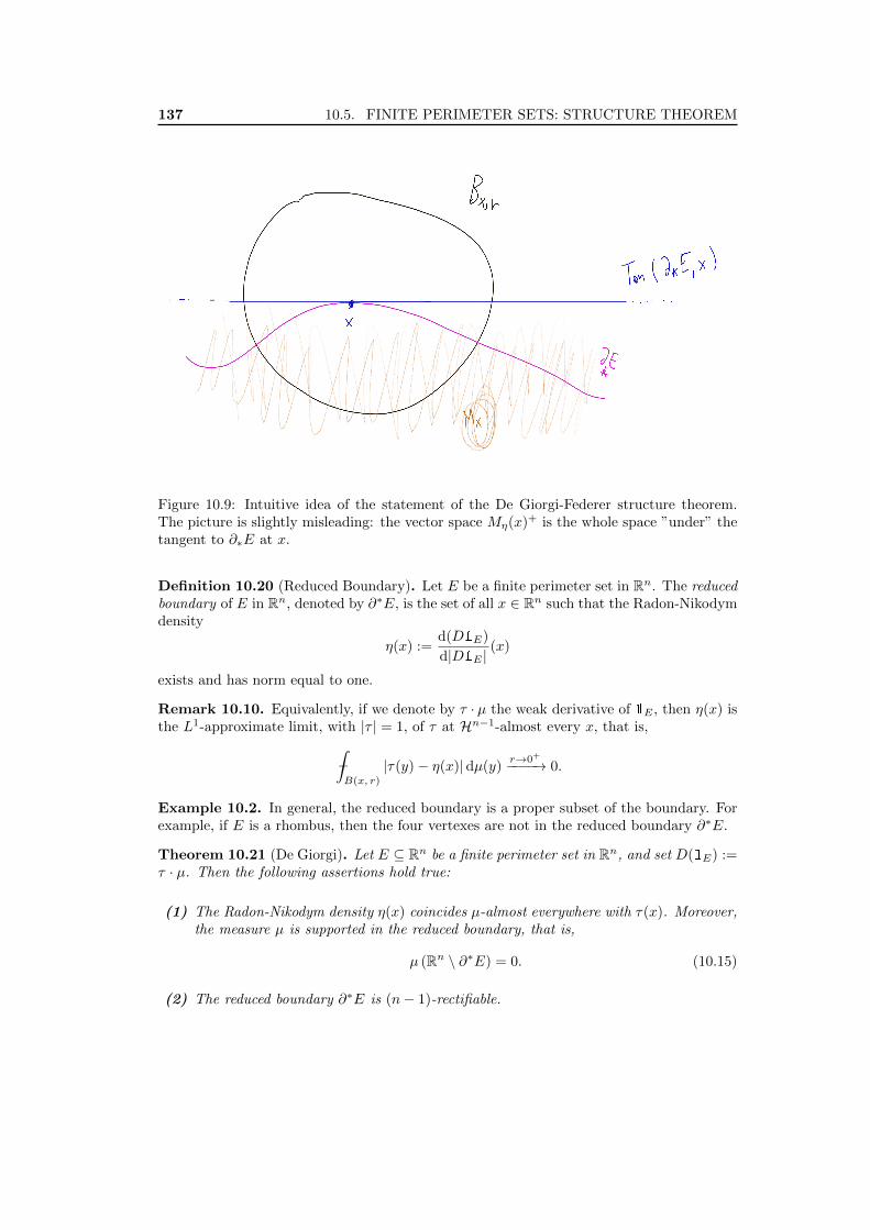
137 10.5. FINITE PERIMETER SETS: STRUCTURE THEOREM
Figure 10.9: Intuitive idea of the statement of the De Giorgi-Federer structure theorem.The picture is slightly misleading: the vector space Mη(x)+ is the whole space ”under” thetangent to ∂∗E at x.
Definition 10.20 (Reduced Boundary). Let E be a finite perimeter set in Rn. The reducedboundary of E in Rn, denoted by ∂∗E, is the set of all x ∈ Rn such that the Radon-Nikodymdensity
η(x) :=d(D1E)
d|D1E |(x)
exists and has norm equal to one.
Remark 10.10. Equivalently, if we denote by τ · µ the weak derivative of 1E , then η(x) isthe L1-approximate limit, with |τ | = 1, of τ at Hn−1-almost every x, that is,
−∫B(x, r)
|τ(y)− η(x)|dµ(y)r→0+
−−−−→ 0.
Example 10.2. In general, the reduced boundary is a proper subset of the boundary. Forexample, if E is a rhombus, then the four vertexes are not in the reduced boundary ∂∗E.
Theorem 10.21 (De Giorgi). Let E ⊆ Rn be a finite perimeter set in Rn, and set D(1E) :=τ · µ. Then the following assertions hold true:
(1) The Radon-Nikodym density η(x) coincides µ-almost everywhere with τ(x). Moreover,the measure µ is supported in the reduced boundary, that is,
µ (Rn \ ∂∗E) = 0. (10.15)
(2) The reduced boundary ∂∗E is (n− 1)-rectifiable.

138 10.5. FINITE PERIMETER SETS: STRUCTURE THEOREM
(3) The measure µ is the restriction of the (n− 1)-dimensional Hausdorff measure to thereduced boundary, that is,
µ = Hn−1 ¬ ∂∗E. (10.16)
(4) The Radon-Nikodym density η(x) is normal to the reduced boundary at x for everyx ∈ ∂∗E, that is,
η(x)⊥ = Tan∗ (∂∗E, x)
where Tan∗ (−, ·) denotes the approximate tangent plane.
(5) The normal vector field η satisfies the following property:
Ln((E4 (x+M+
η(x)))∩Bx, r
) rn as r → 0+ (10.17)
for every x ∈ ∂∗E. Equivalently,
1
r(E − x)
L1loc(R
n)−−−−−→r→0+ M+η(x). (10.18)
Corollary 10.22. Under the assumptions of the Theorem 10.21 it turns out that
Θn(E, x) =1
2
for every x ∈ ∂∗E.
The proof of De Giorgi’s Theorem 10.21 will follow reasonably quickly from a sequenceof many technical lemmas that we will patently state and prove here.
In order to ease the statements of the following results, we will fix a point x ∈ ∂∗E anddenote it by 0 unless otherwise stated.
Lemma 10.23. There exists an universal constant c := c(n) > 0 such that
µ(Br) ≤ c · rn−1. (10.19)
In particular, it turns out that there exists an universal constant c′ := c′(n) > 0 such that
µ(Br) ≤ c′ · Hn−1 (∂Br ∩ E) . (10.20)
Proof. Set Er := E ∩Br.
Step 1. We claim that, for almost every r > 0, the weak derivative of the characteristicfunction satisfies an additive formula:
D(1Er ) = 1Br ·D(1E) + 1E ·D(1Br ). (10.21)
We notice that the integral of η(0) with respect to the measure D(1Er ) is given by∫Rnη(0) dD(1Er ) = 0,

139 10.5. FINITE PERIMETER SETS: STRUCTURE THEOREM
since η(0) is constant. On the other hand, it follows from (10.21) that∫Rnη(0) dD(1Er ) =
∫Br
η(0)η(x) dµ(x) +
∫E
η(0)dD(1Br )(x) =
=
∫Br
η(0)η(x) dµ(x) +
∫∂Br∩E
η(0)νinn(x) dHn−1(x),
where νinn(x) denotes the inner normal vector to the sphere at x. In particular, it turnsout that ∫
Br
η(0)η(x) dµ(x) = −∫∂Br∩E
η(0)νinn(x) dHn−1(x) ≤
≤ Hn−1(∂Br) ∼ αnrn−1,
where the inequality follows from the fact that both νinn and η are vectors of norm less orequal than 1.
In conclusion, we notice that for r → 0+ the left-hand side of the inequality above isasymptotically equivalent to µ(Br), which means that there exists a r0 > 0 small enoughsuch that
1
2µ(Br) ≤
∫Br
η(0)η(x) dµ(x) ≤ Hn−1(∂Br) ∼ c(n) · rn−1,
for almost every 0 < r < r0.
Step 2. We now sketch the proof of the claim (10.21). More precisely, we show that theformula holds for every f.p.s. E and almost every r > 0 - even when 0 does not belong tothe reduced boundary -.
Step 2.1. First, we notice that (10.21) holds for every smooth f.p.s. E that is also transver-sal to the boundary of the ball Br. Indeed, one can easily prove that
∂Er =(∂Br ∩ E
)∪(Br ∩ ∂E
).
Step 2.2. Let En be an approximation of E by smooth sets, that is
EnL1loc−−−→ E.
Choose r > 0 in such a way that ∂Enr is transversal to the sphere ∂Br for every n ∈ N. Theprevious step proves that En satisfies (10.21) for every n ∈ N, which means that we canpass the identity to the limit3.
Lemma 10.24. There are two universal constants c := c(n), c′ := c′(n) > 0 such that forevery r > 0 small enough
c · rn ≤ |E ∩Br| ≤ c′ · rn, (10.22)
andc · rn ≤ |Ec ∩Br| ≤ c′ · rn. (10.23)
3We will not give any detail, but one needs to be careful to the notion of convergence that comes intoplay here.

140 10.5. FINITE PERIMETER SETS: STRUCTURE THEOREM
Remark 10.11. It is easy to prove that the complement of a f.p.s. is also a f.p.s. withthe same weak derivative up to null sets. In particular, the inequality (10.22) implies theinequality (10.23) by passing to the complement.
Proof. Set Er := E ∩Br.
Step 1. We claim that the following isoperimetrical inequality holds: For every r > 0there exists an universal constant c := c(n) > 0 such that
v(r)n−1n ≤ c · Per(Er), (10.24)
where v(r) denotes the Lebesgue measure of Er. If the inequality holds, then it is easy tosee that
v(r)n−1n ≤ c1 · ‖D(1Er )‖ ≤
≤ c2(PerBr (E) +Hn−1 (E ∩ ∂Br)
)≤
≤ c3 · Hn−1 (E ∩ ∂Br) = c3 · v(r),
sincePerBr (E) = |D(1E)|(Br) = µ(Br),
and clearly µ(Br) and Hn−1 (E ∩ ∂Br) are comparable quantities as a consequence of theprevious result.
Step 2. The symbol v denotes the classic derivative of v since a Lipschitz function isalmost everywhere differentiable (by Rademacher Theorem 7.7). The reader may prove, asan exercise, that the formula used above holds:
v(r) = Hn−1 (E ∩ ∂Br) for almost every r > 0. (10.25)
Step 3. In conclusion, we notice that v(r) is an almost everywhere differentiable functionwhich satisfies the following inequality:
v(r)n−1n ≤ c3 · v(r).
A straightforward computation yields to
v(r) ≥ c(n) · rn,
which is exactly the nontrivial part of (10.22). The trivial one, on the other hand, followsimmediately from the worst estimate possible:
v(r) ≤ |Br| ∼ c′(n) · rn.

141 10.5. FINITE PERIMETER SETS: STRUCTURE THEOREM
Step 4. It remains to prove the the claimed isoperimetrical inequality (10.24); surprisingly,it follows easily from a far more general theorem.
Precisely, one can prove that there exists a universal constant c := c(n) such that forany given F bounded f.p.s., it turns out that
|F |n−1n ≤ c(n) · Per(F ).
Recall that the immersionBV(Ω) → L1∗(Ω),
where 1∗ = nn−1 , is continuous (and compact). Therefore, there exists a universal constant
c′ := c′(n) > 0 such that‖u‖
Lnn−1 (Ω)
≤ c′ · ‖u‖BV(Ω).
The reader may prove that one can always replace the BV(Ω)-norm with the total variation‖Du‖ if u is, for example, compactly supported. The isoperimetrical inequality followsimmediately by taking u := 1F for every bounded f.p.s. F .
Lemma 10.25. Let Er := 1r (E − x) = 1
rE. Then
ErL1loc−−−→M+
η(0), (10.26)
or, equivalently, it turns out that∣∣∣(E4M+η(0)) ∩Br
∣∣∣ rn as r → 0+. (10.27)
Proof. Denote by ηr and µr the rescaling of η and µ respectively, in such a way that
D(1Er ) = ηr · µr.
Step 1. By Lemma 10.23 it turns out that
µr(B1) =µ(Br)
rn−1≤ c(n) =⇒ µr(BR) ≤ c(n) ·Rn−1 (10.28)
for every R > 0. Similarly, by Lemma 10.24 it turns out that
c1(n) ≤ |Er ∩B1| ≤ c′1(n),
from which it follows that
c1(n) ·Rn ≤ |Er ∩BR| ≤ c′1(n) ·Rn (10.29)
for every R > 0. The compactness property of the f.p.s. (see Theorem 10.3), together withthe inequality (10.28), imply that, up to subsequences,
1Er
L1loc−−−→ 1E0
D (1Er )locally−−−−→ D (1E0
)

142 10.5. FINITE PERIMETER SETS: STRUCTURE THEOREM
for some f.p.s. E0. Since 0 belongs to the reduced boundary ∂∗E, we have that
−∫Br
|η(x)− η(0)|dµ(x)r→0+
−−−−→ 0,
which means that for every R > 0
−∫BR
|ηr(x)− η(0)|dµr(x)r→0+
−−−−→ 0.
We may assume without loss of generality that η(0) = e1, where e1, . . . , en is the standardorthonormal basis of Rn. It turns out that
D (1E0) = η(0) · µ0,
from which we infer that Di (1E0) is zero for every i = 2, . . . , n.
Step 2. By Lemma 10.26 it turns out that 1E0has a representative which depends only
on the first variable x1, and thus we can infer that
E0 = x0 +M+η(0)
for some x0 ∈ Rn. It remains to prove that x0 is necessarily equal to zero.
We argue by contradiction: suppose that x0 is not 0. Then one can find a radiusR > 0 small enough such that the Lebesgue measure of the intersection E0 ∩BR is zero, incontradiction with the inequality (10.29). Therefore
E0 = M+η(0) and Er
L1loc−−−→ E0 = M+
η(0),
which is exactly what we wanted to prove.
Lemma 10.26. Let f ∈ L1loc(Rn) be a function such that
Dif ≡ 0 ∀ i = 2, . . . , n.
Then there exists f ∈ L1loc(R) such that
f(x1) = f(x1, . . . , xn) for Ln-almost every x = (x1, x2, . . . , xn) ∈ Rn.
Lemma 10.27. Let Er := 1r (E − x) = 1
rE. Then
D(1Er )locally−−−−→ D(1M+
η(0)) = η(0)1η(0)⊥ · Hn−1. (10.30)
Lemma 10.28. For every r > 0 it turns out that
µ(Br) ∼ αn−1rn−1. (10.31)
Proof. We divide the argument into two steps to ease the notation.

143 10.5. FINITE PERIMETER SETS: STRUCTURE THEOREM
Step 1. First, we deduce from Lemma 10.27 that
|D(1Er )|locally−−−−→
∣∣∣D(1M+η(0)
)∣∣∣ . (10.32)
Indeed, if η(0) = e1, then
−∫BR
|ηr(x)− η(0)|dµr(x)r→0+
−−−−→ 0, ∀R > 0
implies that ∣∣∣∣∂ 1Er∂x1
∣∣∣∣ r→0+
−−−−→∣∣∣∣∂ 1E0
∂x1
∣∣∣∣ ,which is exactly what we wanted to prove since E0 = M+
η(0).
Step 2. From (10.32) it follows that4
µ(Br)
rn−1= µr(B1) −−−→ Hn−1(η(0)⊥ ∩B1) = αn−1
for almost every r > 0. To conclude the proof, we need the following auxiliary lemma.
Lemma 10.29. Let (λn)n∈N be a sequence of vector measures on X. Assume that λn :=τn · µn converges in the sense of measures (weakly-∗) to a measue λ := τ · µ, and assumethat there exists a constant vector v such that∫
X
|τn − v|(x) dµn(x)n→+∞−−−−−→ 0.
Then µn converges to µ and λ = v · µ almost everywhere.
We have finally introduced all the technical tools to prove the statements of the DeGiorgi’s theorem presented above.
Proof of Theorem 10.21.
(1) The first statement about the density and the support of µ is an immediate conse-quence of the argument used in the next point.
(2) We sketch two different proofs of the fact that the reduced boundary is (n − 1)-rectifiable. The first proof is due to De Giorgi, while the second one relies more onthe sequence of technical lemmas above.
(a) For every r0 > 0 and δ0 > 0 we consider
Sr0, δ0 :=x ∈ ∂∗E
∣∣∣ ∣∣∣(E4(x+M+η(x))) ∩B(x, r)
∣∣∣ ≤ δ0rn for every r ≤ r0..
4Here the reader needs to be careful. The convergence is not true in general, but one can prove that itis enough to ask that Hn−1(η(0)⊥ ∩B1) = 0.

144 10.5. FINITE PERIMETER SETS: STRUCTURE THEOREM
The idea is to prove that each Sr0, δ0 is (n− 1)-rectifiable. In fact, we know thatthe countable union of d-rectifiable set is also d-rectifiable, and hence the thesisfollows from the fact that
∂∗E =⋃
(n,m)∈N2
S 1n ,m
.
(b) The support of the measure µ is contained in the reduced boundary ∂∗E; henceby Lemma 10.28 we can infer that
µ (B(x, r)) ∼ αn−1rn−1 for µ-almost every x ∈ ∂∗E.
We claim that there exists F ⊆ spt(µ) such that
c1 1F · Hn−1 ≤ µ ≤ c2 1F · Hn−1 and µ (∂∗E \ F ) = 0.
Indeed, it is enough to notice that µ (E \ ∂∗E) = 0 as the support of µ is containedin the reduced boundary. Moreover, the (n−1)-dimensional upper density is zeroat almost every point of F , that is,
Θ∗(µ, x) = 0 for Hn−1-almost every x ∈ F ,
and this implies that Hn−1 (∂∗E \ F ) = 0,
Hn−1 (∂∗E4F ) = 0.
The measure µ is thus equivalent to the restriction of the Hn−1 measure to thereduced boundary, that is, there are two constants c1, c2 > 0 such that
c′1 1∂∗E · Hn−1 ≤ µ ≤ c′2 1∂∗E · Hn−1 =⇒ µ ∼ Hn−1 ¬ ∂∗E.
We deduce that the blowup of µ at x is given by
1η(x)⊥ · Hn−1,
which means that η(x)⊥ is the approximate tangent plane of ∂∗E at x.
Moreover, the lower density is bounded from below; therefore, by Corollary 8.24,we can finally infer that ∂∗E is (n− 1)-rectifiable.
(3) In the previous point we have proved that µ is equivalent to 1∂∗E ·Hn−1, which meansthat there exists a function g such that
µ = 1∂∗E g · Hn−1.
Therefore it is enough to show that g is equal to 1 Hn−1-almost everywhere. The(n− 1)-dimensional upper density of the Hausdorff measure is given by
Θ∗n−1(∂∗E, x) = 1 for Hn−1-almost every x ∈ ∂∗E,
while the (n− 1)-dimensional upper density of µ is given by
Θ∗n−1(µ, x) = 1 for µ-almost every x ∈ ∂∗E.
In particular, it follows that g = 1 almost everywhere (with respect to either µ orHn−1).

145 10.5. FINITE PERIMETER SETS: STRUCTURE THEOREM
(4) This assertion also follows immediately from the second proof of (2).
(5) This assertion simply summarize the content of Lemma 10.25.
We are finally ready to prove the De Giorgi-Federer Theorem 10.16. The reduced bound-ary is a subset of the essential boundary, therefore everything follows from the previous resultif we are able to prove that
Hn−1 (∂∗E \ ∂∗E) = 0.
Proposition 10.30 (Isoperimetrical Inequality). Let E ⊆ Rn be a finite perimeter set inB(x, r). Then there exists an universal constant c := c(n) > 0 such that5
(|E| ∧ |B(x, r) \ E|)n−1n ≤ c · PerB(x, r)(E). (10.33)
Proof. The Sobolev Embedding Theorem implies that the immersion
BV(B(x, r)) → L1∗(B(x, r)),
where 1∗ = nn−1 , is continuous. Therefore, there exists a universal constant c := c(n) > 0
(which does not depend on the radius and the center of the ball) such that
‖u‖L
nn−1 (B(x, r))
≤ ‖u‖BV(B(x, r)).
We replace the BV(B(x, r)) norm with the equivalent one
‖Du‖+
∣∣∣∣∣ −∫B(x, r)
u
∣∣∣∣∣ .It turns out that
‖u− −∫B(x, r)
u‖L
nn−1 (B(x, r))
≤ c(n) ‖Du‖.
By symmetry, we may assume without loss of generality that |E| < |B(x, r) \ E|. Then itis easy to prove that
1E(x)− |E||B(x, r)|
>1
2, if x ∈ E,
and the thesis follows from the inequality above since
c(n) ‖Du‖ ≥ ‖u− −∫B
u‖L
nn−1 (B(x, r))
≥ 1
2|E|
n−1n .
Lemma 10.31. Under the assumptions of the Theorem 10.16, it turns out that
µ (B(x, r)) rn−1 =⇒ Θ∗n(E, x) ∈ 0, 1.
In particular, the point x does not belong to the essential boundary ∂∗E.
5The inequality presented here is not sharp! The result can be refined, but it is not necessary for ourpurposes.

146 10.6. BACK TO THE CAPILLARITY PROBLEM
Proof. Let x ∈ Rn be a point such that Θn(E, x) 6= 0, 1 (i.e., x belongs to the essentialboundary). Then there exists δ > 0 and a sequence (rn)n∈N converging to 0 such that either
∃ (rnk)k∈N : rkk→+∞−−−−−→ 0 and
|E ∩B(x, rnk)|rnnk
≥ δ,
or
∃ (rnk)k∈N : rkk→+∞−−−−−→ 0 and
|E ∩B(x, rnk)|rnnk
≤ αn − δ,
Either way the function
R 3 r 7−→ |E ∩B(x, r)|rn
is continuous; hence there exists λ′ < λ real numbers such that
λ′ ≤ |E ∩B(x, rnk)|rnnk
< λ
for rnkk→+∞−−−−−→ 0. On the other hand, the isoperimetrical inequality (10.33) implies that
|E ∩B(x, r) \ E|n−1n ≤ c · PerB(x, r)(E) = µ (B(x, r)) ,
from which we derive a contradiction with the assumption µ(B(x, r)) rn−1 by noticingthat
λ′rn−1 ≤ |E ∩B(x, r) \ E|n−1n ≤ c · PerB(x, r)(E) = µ (B(x, r))
for every r > 0 small enough.
Lemma 10.32. Under the assumptions of the Theorem 10.16, it turns out that
Hn−1 (∂∗E \ ∂∗E) = 0.
Proof. Equivalently, we may prove that for Hn−1-almost every point x /∈ ∂∗E, it turns outthat x does not belong to ∂∗E as well. By Lemma 10.31, it suffices to prove that
µ (B(x, r)) rn−1,
but this follows easily from the fact that
µ = Hn−1 ¬ ∂∗E.
10.6 Back to the Capillarity Problem
We are finally ready to prove the existence of a solution to the capillarity problem for anyσ ∈ [−1, 1] using the new notion of essential boundary.

147 10.6. BACK TO THE CAPILLARITY PROBLEM
Framework. Fix Ω ⊂ Rn regular bounded open set, and fix a volume
0 < m < |Ω|.
The capillarity energy is given by
F (E) := Hn−1(Σf ) + σHn−1(Σc), (10.34)
where we define Σf := ∂∗E ∩ Ω,
Σc := ∂∗E ∩ ∂Ω.
Theorem 10.33. The functional (10.34) is lower semi-continuous on the set of all finiteperimeter set. Moreover, there exists (at least) a minimum point E for F for every σ ∈[−1, 1].
Proof. We split the proof into two cases: positive and negative σ.
Case ”1 ≤ σ ≥ 0”: The functional (10.34) can be equivalently written as
F (E) = σHn−1(∂∗E) + (1− σ)Hn−1(Σf)
=
= σ · Per(E) + (1− σ) · PerΩ(E).
(10.35)
In particular, the functional (10.35) is equal to the convex sum of two lower semi-continuousfunctionals, which means that it is also lower semi-continuous.
The functional F is also coercive. Indeed, let (En)n∈N ⊂ X be a uniformly boundedsequence, that is, there exists a constant M ∈ R such that
F (En) ≤M, ∀n ∈ N.
Then, up to subsequences, there exists a finite perimeter set E such that EnX−→ E. If σ is
strictly greater than 0, then the perimeters are equibounded
σ · Per(En) ≤ F (En) ≤M,
which means that we can apply a compactness theorem for f.p.s. and conclude that thefunctional is coercive. On the other hand, if σ = 0, then the coerciveness follows immediatelyfrom the following estimate:
Per(En) ≤ Hn−1(∂Ω) + PerΩ(En) ≤ Hn−1(∂Ω) +M < +∞.
Case ”−1 ≥ σ ≤ 0”: The idea is to pass everything to the complement, that is, weconsider as a variable for the functional (10.34) the set Ec := Ω \ E instead of E. Inparticular, we notice that there are nice relations between the surfaces, that is,Σfc = Σf ,
Σcc = ∂Ω \ Σc.

148 10.6. BACK TO THE CAPILLARITY PROBLEM
It turns out that
F (E) = σHn−1(∂Ω)− σHn−1(∂Ω) + F (E) =
= σHn−1(∂Ω) +Hn−1(Σfc ) + |σ|Hn−1(Σcc) =
= F|σ|(Ec) + σHn−1(∂Ω).
(10.36)
Since σHn−1(∂Ω) is a constant, we can immediately reduce to the previous case 1 ≥ |σ| ≥0.
Remark 10.12. The restriction of (10.34) to any smooth subset Ω in X agrees with theclassical capillarity energy presented in the previous section, and the relaxation of F to X isgiven by F itself. Therefore every minimizing sequence, made up of smooth sets, convergesto the minimum of F on X .
Remark 10.13. Up to dimension 8, the inner regularity theory of the capillarity problemworks just fine; the boundary regularity, on the other hand, is quite messy.
Remark 10.14. A similar problem arises when dealing with Plateau’s type problems. Moreprecisely, the surface
Σ = (∂∗Emin) ∩ Ω
is closed (in Ω), and it is also analytic up to dimension 7. As we shall prove at the endof the course, starting from dimension 8, one can find a counterexample to this statement(actually, it is possible to find a minimal surface such that it is analytic outside of a closedsingular set of dimension n− 8).

Chapter 11
Appendix
11.1 First Variation of a Functional
Framework. Let Σ be a d-rectifiable and Hd-finite set in Rn, and let (Φt)t∈R be a oneparameter family of diffeomorphisms of Rn such that Φ0 = idRn . Let
v(x) :=dΦt(x)
dt
∣∣t=0
,
and suppose that Σt := Φt(Σ) is the collection of all the competitors (of Σ) to a certainminimum problem.
Lemma 11.1. Let x ∈ Σ be a point, and let e1, . . . , ed be an orthonormal basis of thetangent space Tan(Σ, x). Then it turns out that
dHd(Σt)dt
∣∣t=0
=
∫Σ
divT (v)(x) dHd(x), (11.1)
where divT (−) denotes the divergence along the tangent plane, that is,
divT (v)(x) =
d∑i=1
∂ (〈v, ei〉)∂ei
(x).
Proof. The map Φt is a diffeomorphism for every t; hence we can apply the area formula(7.6) to Σt, and obtain the following identity:
Hd (Σt) =
∫Σ
JT (Φt)(x) dHd(x), (11.2)
where JT denotes the tangential Jacobian, that is,
JT (Φt) =√
det ((∇TΦt)t(∇TΦt)).
Fix x ∈ Σ. By Taylor’s expansion theorem one can prove thatΦt(x) = x+ t v(x) +Ox(t),
dΦt(x) = Id + tdv(x) +Ox(t).

150 11.1. FIRST VARIATION OF A FUNCTIONAL
Let e1, . . . , en be an orthonormal basis of Rn such that e1, . . . , ed is an orthonormalbasis of the tangent space Tan(Σ, x). Then we can write the relations above as follows:
∇TΦt =
[Idd×d 0
0 0
]+ t
(∇T v
0
)+Ox(t).
If we refer to the first matrix on the right-hand side by J , then it is easy to prove that
(∇TΦt)t(∇TΦt)(x) = Idd×d(x) + t
(J t∇T v(x) + (∇T v(x))
tJ)
+Ox(t),
from which it follows that
JT (Φt)(x) =√
det ((∇TΦt)t(∇TΦt)) '
'√
1 + t · tr(J t∇T v(x) + (∇T v(x))
tJ)
+Ox(t) =
=√
1 + 2tdivT (v)(x) +Ox(t) '
' 1 + tdivT (v)(x) +Ox(t),
where the first approximation ' follows from the Taylor’s expansion
det(Idn×n + tA) ' 1 + tTr(A) + o(t) as t→ 0,
and the last approximation follows from the Taylor’s expansion of√
1 + x. In particular, itturns out that∫
Σ
JT (Φt)(x) dHd(x) =
∫Σ
(1 + tdivT (v)(x) +Ox(t)) dHd(x) =
= Hd(Σ) + t
∫Σ
divT (v)(x) dHd(x) + o(t).
Notice that the remainder needs a reasonable assumption to behave properly: For example,we can require either Σ bounded or Φt is the identity outside of a compact set K for everyt ∈ R.
In conclusion, it is enough to take the derivative with respect to the time of (11.2), andevaluate it at t = 0, to obtain exactly the sought formula (11.1).
Theorem 11.2 (Divergence Theorem). Let Σ be a compact (d − 1)-dimensional surfacewith a boundary ∂Σ of class C2. Then
d
dtHd−1(Σt)
∣∣t=0
= −∫
Σ
~H(x)v(x) dHd−1(x) +
∫∂Σ
η∂Σ(x)v(x) dHd−2(x), (11.3)
where ~H(x) is the mean curvature vector of Σ at x and η∂Σ is the outward normal of ∂Σ atx.
Lemma 11.3. Let Σ0 ⊂ Rn be a hypersurface which minimizes the area (the (n − 1)-dimensional volume) among all Σ such that
Σ4Σ0 ⊂⊂ Ω,
where Ω is a fixed open set in Rn. Then
~HΣ0(x) = 0, ∀x ∈ Ω ∩ Σ0.

151 11.1. FIRST VARIATION OF A FUNCTIONAL
Proof. Let v be a compactly supported smooth vector field on Ω. Then there exists a family(Φt)t∈I of diffeomorphisms with v as initial speed1 and Φ0 = idRn . It turns out that thehypersurfaces (Σt)t∈I := (Φt(Σ0))t∈I are all competitors for the area problem; hence thefunction
t 7−→ Hn−1(Σt)
has a (local) minimum at t = 0. From the divergence formula (11.3) we obtain the relation
d
dtHn−1(Σt)
∣∣t=0
= 0 =⇒∫
Σ
~HΣ0(x)v(x) dHn−1(x) = 0,
since the boundary term is equal to zero. Therefore, a straightforward application of thefundamental lemma in calculus of variation allows us to infer that
~HΣ0(x) = 0, ∀x ∈ Ω ∩ Σ0.
Remark 11.1. If Σ is a finite perimeter set, then a similar computation shows that∫∂∗Σ
divT (v) = 0,
which means that we cannot choose any smooth vector field v when dealing with it.
We can summarize the results obtained in this section with a slightly different version ofthe divergence formula (11.3), which holds for every smooth vector field v.
Proposition 11.4. Let Σ be a compact (n−1)-dimensional (hyper)surface with a boundary∂Σ of class C2. Then∫
Σ
divT (v)(x) dHn−1(x) = −∫
Σ
~H(x)v(x) dHn−1(x) +
∫∂Σ
η∂Σ(xv(x) dHn−2(x) (11.4)
for every2 v ∈ C∞(Rn).
Proof. We can decompose the vector field as follows:
v = vN · η∂Σ + vT ,
where vN is the normal component, and vT is the tangential component. Then one caneasily check that the following identity holds:
divT (v) = divT (vN )
=0
·η∂Σ + vN · divT (η∂Σ) + divT (vT ).
We notice that divT (η∂Σ) is the trace of the second fundamental form, which means that
divT (η∂Σ) = | ~H|(x) =: H(x).
1For example, the reader may consider the family of diffeomorphisms Φt(x) := x + t v(x), which iswell-defined in a small neighborhood of 0.
2Here we can take any smooth vector field v because Σ is compact by assumption. If not, then v needsto be a compactly supported vector field.

152 11.1. FIRST VARIATION OF A FUNCTIONAL
The usual divergence theorem for a smooth vector field gives us the identity∫Σ
divT (v) dHn−1(x) =
∫∂Σ
v(x)η∂Σ(x) dHn−2(x).
If we plug the first relation (for the divergence) into the second one (divergence theorem forsmooth functions), then it turns out that∫
Σ
divT (v)(x) dHn−1(x) = −∫
Σ
~H(x)v(x) dHn−1(x) +
∫∂Σ
η∂Σ(x)v(x) dHn−2(x),
which is exactly what we wanted to prove.
Remark 11.2. Let Σ ⊂ Rn be a compact (n− 1)-dimensional surface with a boundary ∂Σ
of class C2. If Σ minimizes the (n− 1)-dimensional volume among all Σ such that(Σ4Σ
)∩ ∂Σ = ∅,
then the mean curvature ~HΣ is identically equal to 0.
We can state and prove a similar result for finite perimeter sets, but first we need a tech-nical result concerning the closure of BV(Ω) with respect to the action of a diffeomorphism.
Lemma 11.5. Let Ω be a fixed open set in Rn, and let Φ be a diffeomorphism of Ω. Ifu ∈ BV(Ω), then the composition u Φ−1 also belongs to BV(Ω).
Lemma 11.6. Let Ω be a fixed open set in Rn, and let E be a finite perimeter set whichminimizes the perimeter inside Ω among all E f.p.s. in Ω such that
E4 E ⊂⊂ Ω
up to null sets. Then it turns out that∫∂∗E
divT (v) dHn−1 = 0, ∀ v ∈ C∞c (Ω).
Proof. Fix v compactly supported smooth vector field on Ω. Then there exists a family(Φt)t∈I of diffeomorphisms with v as initial speed3 and Φ0 = idRn . Since Φt(x) = x for everyx which does not belong to the support of v, Lemma 11.6 proves that (Et)t∈I := (Φt(E0))t∈Iis a collection of finite perimeter set such that
∂∗Et = Φt(∂∗E).
In particular, the f.p.s. Et are all competitors for the perimeter problem; hence the function
t 7−→ PerΩ(Et)
admits a (local) minimum at t = 0. The thesis follows from a simple identity which is leftto the reader:
d (PerΩ(Et))
dt
∣∣t=0
=
∫∂∗E
divT (v) dHn−1.
3For example, the reader may consider the family of diffeomorphisms Φt(x) := x + t v(x), which iswell-defined in a small neighborhood of 0.

153 11.1. FIRST VARIATION OF A FUNCTIONAL
Definition 11.7 (Weak Mean Curvature). Let Σ be a d-rectifiable set in Rn. We say thatΣ has mean curvature in the weak sense if and only if there exists ~g ∈ Lp
(Rn, Hd ¬Σ
)such
that ∫Σ
divT (v)(x) dHd(x) =
∫Σ
~g(x)v(x) dHd(x), ∀ v ∈ C∞c (Rn).
Remark 11.3. Let Σ be a compact (n − 1)-dimensional (hyper)surface with a boundary∂Σ of class C2. If Σ admits a weak mean curvature ~g, then the following properties hold:
(i) The weak mean curvature ~g coincides with the mean curvature ~H almost everywhere.
(ii) The boundary of Σ is empty4.
Definition 11.8 (k-Varifold). An integral k-dimensional varifold is a couple (Σ, θ), whereΣ is a k-rectifiable set in Rn, and θ : Σ −→ N is a function in L1
(Rn, Hk ¬Σ
).
Definition 11.9 (Varifold W.M.C.). Let (Σ, θ) be a k-dimensional varifold in Rn. We saythat Σ has mean curvature in the weak sense if and only if there exists ~g ∈ Lp
(Rn, Hd ¬Σ
)such that∫
Σ
θ(x)divT (v)(x) dHk(x) =
∫Σ
θ(x)~g(x)v(x) dHk(x), ∀ v ∈ C∞c (Rn).
Exercise 11.1. Let Σ be a compact (n − 1)-dimensional (hyper)surface with a boundary∂Σ of class C2, and let θ ∈ BV(Σ; N). Suppose that∫
Σ
θ(x) div(v)(x) dHk(x) = −∫
Σ
v(x) dθ(x)
for every tangent vector field v ∈ C∞c (Σ). Prove that:
(i) The weak mean curvature ~g coincides with the mean curvature ~H almost everywhere.
(ii) The boundary of Σ is empty.
(iii) The function θ is locally constant.
Exercise 11.2. Let Σ be a compact (n − 1)-dimensional (hyper)surface with a boundary∂Σ of class C2, and let θ ∈ C∞(Σ; R). Suppose that∫
Σ
θ(x) div(v)(x) dHk(x) = −∫
Σ
v(x) dθ(x)
for every tangent vector field v ∈ C∞c (Σ). Prove or disprove the following formula:
~g = ~H − ∇T θθ
.
4This follows fairly easily from the integration by parts formula.

154 11.2. REGULARITY IN CAPILLARITY PROBLEMS
11.2 Regularity in Capillarity Problems
Framework. Let Ω ⊂ Rn be an open bounded subset of Rn. In this section, we shalldiscuss the capillarity problem equilibrium when the container (Ω) is fixed and the volumeof the liquid is fixed. More precisely, the drop of liquid (denoted by E), contained in Ω,is at equilibrium if and only if it is a critical point (local minima) of the capillarity energyfunctional
F (E) := Hn−1 (∂E ∩ Ω) + σHn−1 (∂E ∩ ∂Ω) , (11.5)
where σ ∈ R is a constant, subject to the constraint that the volume is fixed, e.g. |E| = m.
Mean Curvature. Assume that E is a f.p.s. which minimizes the capillarity energy (11.5)and satisfies the constraint on the volume. If E is regular enough, then one can prove thatHf is constant on the free portion of the surface Σf ,
θY is constant on the boundary Γ.
More precisely, the free mean curvature Hf is the Lagrange multiplier associated to thevolume constraint, while θY is the solution of the trigonometric equation
cos θY = −σ. (11.6)
The first assertion is easy to prove. Let (Φt)t∈I be a family of diffeomorphisms fixing theboundary, and choose a smooth vector field v in such a way that the volume constraint isnot violated, that is,
the constraint is preserved ⇐⇒∫
Σfv · η = 0,
which means that the first variation of the volume is zero. As a result of the technical toolsintroduced in the previous section, it turns out that if we set the first variation equal tozero, then we obtain ∫
ΣfH(v · η) = 0, ∀ v ∈ C∞c :
∫Σfv · η = 0.
The Du Bois-Reymond’s fundamental lemma in calculus of variation allows us to infer that
H∣∣Σf
= c =⇒ Hf = c,
that is, the free mean curvature is constant. The proof of (11.6) is very similar, but we needto consider a family of transformations which moves the boundary.
Remark 11.4. If E is not regular enough, then one might translate the problem in thesetting of k-varifolds, and prove that the weak mean curvature is constant on Σf . Unfor-tunately, it is not easy at all to give a meaning to θ, and recover something like formula(11.6).

155 11.3. REGULARITY IN THE F.P.S. SETTING
11.3 Regularity in the F.P.S. Setting
Introduction. Let Ω ⊂ Rn be an open bounded subset of Rn, and let E be a finiteperimeter set in Ω minimizing the perimeter PerΩ(−) among all f.p.s. E such that
E4 E ⊂⊂ Ω.
Theorem 11.10. The essential boundary ∂∗E is closed in Ω, and there is a representativeof E in its equivalence class which satisfies the following properties:
(a) The topological boundary ∂E coincides with the essential boundary ∂∗E.
(b) The perimeter formula is satisfies, that is,
PerΩ(E) = Hn−1(∂E).
Moreover, the representative above can be uniquely characterized as follows:
E = x ∈ E |Θ(E, x) = 1 .
Lemma 11.11. There exists a universal constant δ0 := δ0(n) > 0 such that for every(x0, r0) ∈ Ω× R satisfying B(x0, r0) ⊂ Ω, it turns out that
|E ∩B(x0, r0)|αnrn0
≤ δ0 =⇒∣∣∣E ∩B (x0,
r0
2
)∣∣∣ = 0,
|E ∩B(x0, r0)|αnrn0
≥ 1− δ0 =⇒∣∣∣E ∩B (x0,
r0
2
)∣∣∣ = |B(x0, r0)| ,
almost everywhere.
Truncation Argument. Fix (x0, r0) ∈ Ω× R. For every r ∈ [ r02 , r0], set
Er := E \B(x0, r).
Step 1. The set E minimizes the perimeter; hence
PerΩ(Er) ≥ PerΩ(E).
The usual isoperimetrical inequality yields to5
c(n) |E ∩B(x0, r)|1−1n ≤ PerB(x0, r)(E) =
= Hn−1 (∂∗E ∩B(x0, r)) ≤
≤ Hn−1 (E ∩ ∂B(x0, r))
5The last inequality needs to be justified. The reader should check very carefully the details since a lotof issues could arise here.

156 11.3. REGULARITY IN THE F.P.S. SETTING
for almost every r ∈ [ r02 , r0]. Recall that
D(1Er ) = 1Ω\B(x0, r)D(1E) + ν 1E∩∂B(x0, r) · Hn−1,
from which it follows that
∂∗Er =(∂∗E \B(x0, r)
)∪ (E ∩ ∂B(x0, r))
for almost every admissible r.
Step 2. Let v(r) := |E ∩B(x0, r)| be the n-dimensional Lebesgue measure. Then6
v(r) = Hn−1 (E ∩ ∂B(x0, r)) for a.e. admissible r.
It follows from the isoperimetrical inequality that
c(n) v(r)1− 1n ≤ v(r),
from which it follows that7
v (r0)1n − v
(r0
2
) 1n ≥ c(n)
n
r0
2.
If we rearrange the inequality, then we obtain the following estimate:
v(r0
2
) 1n ≤
[α
1nn
(v(r0)
αnrn0
) 1n
− c(n)
2n
]r0.
In particular, the thesis follows by choosing the universal constant δ0 in such a way thatv(r0/2) is either 0 or equal to the volume of the ball, that is,
δ0 =1
αn
(c(n)
2n
)n.
Proof of Theorem 11.10. Everything is obvious except the fact that ∂∗E is a closed set; weshall show that the complement is open.
Case 1. Fix a point x0 with density Θ(E, x0) equal to 0. Then there exists r0 > 0 smallenough such that
|E ∩B(x0, r0)|αnrn0
≤ δ0,
and thus by Lemma 11.11 it turns out that∣∣∣E ∩B (x0,r0
2
)∣∣∣ = 0.
In particular, it turns out that
Θ(E, x) = 0 ∀x ∈ E ∩B(x0,
r0
2
).
6Here the reader needs to be extremely careful. A priori v is simply differentiable in the weak sense ofdistributions, while in the computation above we need to deal with the classical derivative of v.
7To solve the differential inequality one needs to divide by v. If v(r) 6= 0 for a.e. admissible r, theneverything is fine. On the other hand, if v(r) = 0 in the middle of the interval, then one needs to check thatv is strictly increasing, and thus r : v(r) = 0 is a null set.

157 11.4. STRUCTURE OF FINITE LENGTH CONTINUA IN RN
Case 2. Fix a point x0 with density Θ(E, x0) equal to 1. Then there exists r0 > 0 smallenough such that
|E ∩B(x0, r0)|αnrn0
≥ 1− δ0,
and thus by Lemma 11.11 it turns out that∣∣∣E ∩B (x0,r0
2
)∣∣∣ =∣∣∣B (x0,
r0
2
)∣∣∣ .In particular
Θ(E, x) = 1 ∀x ∈ E ∩B(x0,
r0
2
),
which means that the complement of ∂∗E is open (i.e., ∂∗E is closed).
Exercise 11.3. What happens if the f.p.s. E minimizes the perimeter PerΩ(−) among all
f.p.s. E such thatE4 E ⊂⊂ Ω,
subject to a volume constraint? Is ∂∗E still closed?
11.4 Structure of Finite Length Continua in Rn
The main goal of this section is to prove that a continua (= compact and connected) set Kin Rn with finite length is the image of a surjective path γ such that
Length(γ) ≤ 2 · H1(K) < +∞.
Definition 11.12. Let I := [a, b]. A continuous path γ : I −→ Rn of finite length hasconstant speed c if and only if
Length(γ, J) < c · Length(γ, I)
for every J ⊂ I.
Remark 11.5 (Arc Length). Let γ : I −→ Rn be a continuous path of finite length L. Ifwe set
σ(s) := inf t ∈ [a, b] | Length (γ, [a, t]) ≥ Ls ,
then the riparametrization γ σ : [0, 1] −→ Rn is a continuous path with constant speed L.
Remark 11.6 (Tangent Plane). Let K be a continua set in Rn. Then the tangent planeTan(K, x) is the vector space in the classical sense for H1-almost every x.
Lemma 11.13. Let K be a continua set in Rn with finite length. Then K is connected byarcs and, more precisely, it is connected by injective paths of finite length.
Sketch of the Proof. The main idea is to obtain the injective path γ as the uniform limit(with respect to the Hausdorff distance) of a sequence of finite length paths γδ satisfyingcertain properties.

158 11.4. STRUCTURE OF FINITE LENGTH CONTINUA IN RN
Step 1. Fix x0, x ∈ K. For every δ > 0 we may consider the (almost) shortest δ-chain ofpoints xδ0, . . . , x
δn ∈ K and times 0 =: tδ0 ≤ · · · ≤ tδn := 1, where n depends on δ, such that
the following properties hold:
i) The first point is x0 := xδ0, and the final point is x := xδn for every δ > 0.
ii) The distance between two consecutive points is less than δ, that is,
|xδi − xδi−1| < δ,
and the total length is less than the length of K, that is,
n∑i=1
|xδi − xδi−1| < H1(K).
iii) For every i = 1, . . . , n it turns out that γδ reaches the point xδi at the time tδi .
iv) The Lipschitz constant of γδ is less or equal than 4 times its length.
The reader may prove that the curve γ can be obtained as the uniform limit of the sequence(γδ)δ>0.
Theorem 11.14. Let K be a continua set in Rn with finite length. Then there exists asurjective path γ : [0, 1] −→ K such that
Length(γ) ≤ 2 · H1(K) < +∞.
In particular, every continua H1-finite set is rectifiable.
Proof. The assertion is an immediate consequence of Lemma 11.13.
Remark 11.7 (Degree). The degree of γ at x, which will be denoted by deg(γ, x), is well-defined for H1-almost every x. In particular, for every vector field v ∈ C∞c (Rn; Rn), itturns out that ∫
v(γi(s)) γi(s) ds = 0
for every i ∈ N, which means that∫v(γ(s)) γ(s) ds = 0, ∀ v ∈ C∞c (Rn; Rn).
Since v(γn) converges uniformly to v(γ) and γn converges to γ in L∞w∗ (i.e., in the weak-∗topology of L∞), then the area formula implies that
0 =
∫v(γ(s))
γ(s)
|γ(s)|J(γ)(s)ds =
∫K
v(x)∑
s∈γ−1(x)
τ(s) · deg(γ, x) dH1(x),
where
τ(s) :=γ(s)
|γ(s)|indicates the orientation of the curve. In particular, it turns out that
τ(x) · deg(γ, x) = 0
for H1-almost every x, which means that the cardinality of the set γ−1(x) is even for H1-almost every x.

159 11.5. LOWER SEMI-CONTINUITY: GOLAB THEOREM
11.5 Lower Semi-Continuity: Golab Theorem
In this brief section, we use the structure theorem of a continua set to prove the famousGolab compactness result.
Theorem 11.15 (Golab). Let (Ki)i∈N be a sequence of continua sets in Rn. If Ki convergesto a continua set K with respect to the Hausdorff distance, then
lim infi→+∞
H1(Ki) ≥ H1(K).
Proof. By Theorem 11.14 for every i ∈ N there exists a surjective path γi of finite lengththat parametrizes the corresponding continua set Ki. Up to subsequences, it turns out thatγi converges to some path γ, which parametrizes K.
The preimage γ−1(x) is nonempty, and its cardinality is even (see Remark 11.7). There-fore, one can easily infer that∣∣γ−1(x)
∣∣ ≥ 2 at H1-almost every x ∈ K,
which means that
H1(K) ≤ 1
2· Length(γ).
The length is a semi-lower continuous functional
Length(γ) ≤ lim infi→+∞
Length(γi),
and by Theorem 11.14 it turns out that
Length(γ) ≤ lim infi→+∞
Length(γi) ≤ 2 lim infi→+∞
H1(Ki).
If we combine the two inequalities, then we obtain the thesis:
H1(K) ≤ 1
2· Length(γ) ≤ lim inf
i→+∞H1(Ki).
11.6 Simons’ Cone
In this final section, we show that the minimality of the functional Hn−1(− ∩K) may beachieved via a calibration. We shall apply this result to prove the minimality of the Simons’Cone, which is a singular surface, in dimension n = 8.
Theorem 11.16 (Minimality through Calibration). Let Σ0 be a compact (n−1)-dimensionalhypersurface in Rn with boundary ∂Σ0 oriented by a continuous unit normal η0. Assumethat there exists a calibration for Σ0, that is, a vector field v, defined on the space Rn, withthe following properties:
(i) The vector field v coincides with η0 on Σ0.

160 11.6. SIMONS’ CONE
(ii) The norm of v is less than or equal to 1.
(iii) The divergence of v is identically zero.
Then Σ0 is the hypersurface minimizing the functional Hn−1(−) among all the (n − 1)-dimensional hypersurfaces Σ with the same boundary, oriented in the same way.
Proof. A straightforward computation shows that
Hn−1(Σ0) =
∫Σ0
v · η0 dHn−1 =
=
∫Σ
v · η0 dHn−1 ≤
≤ Hn−1(Σ),
where the blue equality follows from (i), and the red follows from (ii), (iii), and the diver-gence theorem.
Theorem 11.17 (Minimality through Calibration, II). Let Σ0 be a complete (n − 1)-dimensional hypersurface in Rn without boundary. Assume that there exist a Borel set Eand a calibration for Σ0, that is, a vector field v, defined on the space Rn, with the followingproperties:
(i) The vector field v coincides with η0 on Σ0.
(ii) The norm of v is less than or equal to 1.
(iii) The divergence of v is less than or equal to zero in E, and greater than or equal tozero in the complement Rn \ E.
(iv) The surface Σ0 is the boundary of E, and η0 is the outwards normal.
Then Σ0 is the hypersurface minimizing the functional Hn−1(−∩K) among all the (n− 1)-dimensional hypersurfaces Σ which agrees with Σ outside of a compact set K.
Simons’ Cone. The surface
ΣS :=
(x, y) ∈ R4 × R4 | |x| = |y|
admits a calibration v. In particular, the Simons’ cone is the minimal surface (with respectto the (n − 1)-dimensional Hausdorff measure) in dimension n = 8, and it is easy to provethat the origin (0, 0) is a singular point (as stated in the final remark of the previouschapter). We will not present a proof here, but the calibration is given by
v(x, y) :=∇f(x, y)
f(x, y), where f(x, y) =
|x|4 − |y|4
4,
and the Borel set E is given by
E :=
(x, y) ∈ R4 × R4 | |x| < |y|.

Index
approximate tangent cone, 99approximate tangent plane, 92approximately continuous function, 53
Besicovitch Covering Lemma, 40Besicovitch Covering Theorem, 42bounded variation, 105
alternative definition, 108
Caratheodory measurable, 16Caratheodory Theorem, 16cone, 92
essential boundary, 131
fine cover, 37finite perimeter set, 117
relative, 117
Hausdorff dimension, 27Hausdorff measure, 23
upper density, 45Hausdorff spherical measure, 26Hutchinson Theorem, 63
Lipschitz boundary, 109Lipschitz map, 75
Ascoli-Arzela Theorem, 75Kirszbraun Theorem, 76Mc Shame Theorem, 76
measure, 9asymptotically doubling, 44Banach-Alaoglu, 11convergence in variation, 15density, 44doubling, 36integralgeometric, 69invariant, 72locally finite, 36mass, 9orthogonal, 50
outer measure, 16push-forward, 71support, 50tightness, 14total variation, 9vector-valued, 9weak-∗ convergence, 11
open set condition (OSC), 63
purely unrectifiable set, 88
Rademacher Theorem, 77rectifiable set, 85reduced boundary, 132Riesz Theorem, 10
self-similar set, 62set diameter, 21Sobolev critical exponent, 112Sobolev Embedding Theorem, 112space-filling curve, 8strong tangent plane, 92
tangent bundle, 91tangent cone, 97trace theorem, 114
universally measurable, 21
varifold, 147Vitali Covering Lemma, 35Vitali Covering Theorem, 36
weak mean curvature, 147varifold, 147
161

Bibliography
[1] Alexei A. Tuzhilin Alexander O. Ivanov. Minimal NetworksThe Steiner Problem andIts Generalizations. CRC Press, 1994.
[2] Renato Caccioppoli. Sulla quadratura delle superfici piane e curve. Atti Accad. Naz.Lincei Rnd. Cl. Sci. Fis. Mat. Natur., 6:142–146, 1927.
[3] Jesse Douglas. Solution of the problem of plateau. Transactions of the AmericanMathematical Society, 33(1):263–321, 1931.
[4] K. J. Falconer. The Geometry of Fractal Sets. Cambridge University, New York, NY,USA, 1986.
[5] Hebert Federer. Geometric Measure Theory. Classics in Mathematics. Springer-VerlagBerlin Heidelberg, 1 edition, 1996.
[6] Herbert Federer and Wendell H. Fleming. Normal and integral currents. Annals ofMathematics, 72(3):458–520, 1960.
[7] Ennio De Giorgi. Definizione ed espressione analitica del perimetro di un insieme. AttiAccad. Naz. Lincei Rnd. Cl. Sci. Fis. Mat. Natur., 14:29–41, 1953.
[8] Pertti Mattila. Geometry of Sets and Measures in Euclidean Spaces. Cambriidge studiesin advanced mathematics. Cambridge University, 1995.
[9] E. R. Reifenberg. Solution of the plateau problem form-dimensional surfaces of varyingtopological type. Acta Mathematica, 104(1):1–92, 1960.
[10] Harold R. Parks Steven G. Krantz. Geometric Integration Theory. Cornerstones, 2008.
162


![Boundary measures for geometric inferencequentin.mrgt.fr/files/research/boundary.pdfferential geometry [21] and geometric measure theory [14]. In this paper, we show that they can](https://static.fdocuments.us/doc/165x107/5f43550272bd1f247f191f20/boundary-measures-for-geometric-ferential-geometry-21-and-geometric-measure-theory.jpg)