Lecture Notes for the Course on Unit-6 - Neutron Transport Theory
74
NMNR-Unit-5 – Neutron Transport Theory Fundamentals and Solution Methods – Part 2 1 Lecture Notes for the Course on NUMERICAL METHODS FOR NUCLEAR REACTORS Prof. WALTER AMBROSINI University of Pisa, Italy Unit-6 - Neutron Transport Theory Fundamentals and Solution Methods – Part 2 NOTICE: These notes were prepared by Prof. Ambrosini mainly on the basis of the material adopted by Prof. Bruno Montagnini for the lectures he held up to years ago, when he left to Prof. Ambrosini the charge of the course held for the Degree in Nuclear Engineering at the University of Pisa. This material is freely distributed to Course attendees or to anyone else requesting it. It has not the worth of a textbook and it is not intended to be an official publication. It was conceived as the notes that the teacher himself would take of his own lectures in the paradoxical case he could be both teacher and student at the same time (sometimes space and time stretch and fold in strange ways). It is also used as slides to be projected during lectures to assure a minimum of uniform, constant quality lecturing, regardless of the teacher’s good and bad days. As such, the material contains reference to classical textbooks and material whose direct reading is warmly recommended to students for a more accurate understanding. In the attempt to make these notes as original as feasible and reasonable, considering their purely educational purpose, most of the material has been completely re-interpreted in the teacher’s own view and personal preferences about notation. In this effort, errors in details may have been introduced which will be promptly corrected in further versions after discovery. Requests of clarification, suggestions, complaints or even sharp judgements in relation to this material can be directly addressed to Prof. Ambrosini at the e-mail address: [email protected]
Transcript of Lecture Notes for the Course on Unit-6 - Neutron Transport Theory

NMNR-Unit-5 – Neutron Transport Theory Fundamentals and Solution Methods – Part 2 1
Lecture Notes for the Course on
NUMERICAL METHODS FOR NUCLEAR REACTORS
Prof. WALTER AMBROSINI
University of Pisa, Italy
Unit-6 - Neutron Transport Theory Fundamentals
and Solution Methods – Part 2
NOTICE: These notes were prepared by Prof. Ambrosini mainly on the basis of the material adopted by Prof. Bruno
Montagnini for the lectures he held up to years ago, when he left to Prof. Ambrosini the charge of the course held for
the Degree in Nuclear Engineering at the University of Pisa. This material is freely distributed to Course attendees or to
anyone else requesting it. It has not the worth of a textbook and it is not intended to be an official publication. It was
conceived as the notes that the teacher himself would take of his own lectures in the paradoxical case he could be both
teacher and student at the same time (sometimes space and time stretch and fold in strange ways). It is also used as
slides to be projected during lectures to assure a minimum of uniform, constant quality lecturing, regardless of the
teacher’s good and bad days. As such, the material contains reference to classical textbooks and material whose direct
reading is warmly recommended to students for a more accurate understanding. In the attempt to make these notes as
original as feasible and reasonable, considering their purely educational purpose, most of the material has been
completely re-interpreted in the teacher’s own view and personal preferences about notation. In this effort, errors in
details may have been introduced which will be promptly corrected in further versions after discovery. Requests of
clarification, suggestions, complaints or even sharp judgements in relation to this material can be directly addressed to
Prof. Ambrosini at the e-mail address: [email protected]
NMNR-Unit-5 – Neutron Transport Theory Fundamentals and Solution Methods – Part 2 2
SPATIAL ASYMPTOTIC APPROXIMATIONS
FOR THE SPHERICAL HARMONICS METHOD
The plane case with dependence on energy
• Taking into account the dependence on energy, the transport
equation for the plane case is: ( )
( ) ( ) =µφΣ+∂
µφ∂µ ,,,
,,ExEx
x
Ext
( ) ( ) ( ) ( )µ+µ′µ′′φµ→′Σϕ′′π
+= ∑ ∫ ∫ ∫
∞
=
π
−,,,,,
4
12
0
0
2
0
1
1ExSdExPEExdEd
l
l
lsl
• Making use of mathematical developments similar to the ones
adopted for the monokinetic case and assuming
( ) ( ) ( )∑∞
=
µφπ
+=µφ
0
,4
12,,
m
mm PExm
Ex with ( ) ( ) ( )∫− µµµφπ=φ1
1,,2, dPExEx mm
( ) ( ) ( )∑∞
=
µπ
+=µ
0
,4
12,,
m
mm PExSm
ExS with ( ) ( ) ( )∫− µµµπ=1
1,,2, dPExSExS mm
it is possible to reach the energy dependent spherical harmonics
form (we omit the demonstration) ( ) ( )
( ) ( )ExExx
Ex
l
l
x
Ex
l
llt
ll ,,,
12
1,
12
11 φΣ+∂
φ∂
+
++
∂
φ∂
++−
( ) ( ) ( )ExSEdExEEx llsl ,,, +′′φ→′Σ= ∫ ( )...,1,0=l
being a system of infinite integrodifferential equations in ( )Exl ,φ
• The PN approximation consists in truncating the series at the ( )1+N -
th term obtaining 1+N equations ( Nl ...,,1,0= )
Asympotitc spatial dependence for PN and the BN approximations
• In the case of homogeneous regions it is possible to adopt a
procedure different from the spatial discretization, based on a
simple asymptotic approximation
• In the case of calculations aimed to provide the fine group energy
spectrum, a spatial trend of the flux of exponential type (for non
multiplying media) or sinusoidal one (for multiplying media) may
roughly represent the effect of leakages

NMNR-Unit-5 – Neutron Transport Theory Fundamentals and Solution Methods – Part 2 3
• Therefore, for a multiplying medium an imaginary exponential
trend is accepted. The imaginary exponential is more convenient
from a mathematical point ot view than a sinusoidal one, just taking
care to consider only the real part of both the flux and the source
(assumed to be isotropic)
( ) ( ) xiBeEEx
−µϕ=µφ ,,, ( ) ( ) xiBeESExS
−
π=µ 0
4
1,,
• As a consequence, for the coefficients of the Legendre polynomials
it is
( ) ( ) xiBnn eEEx
−ϕ=ϕ ,
• With these definitions, substituting into the relation ( ) ( ) ( )µφΣ+
∂
µφ∂µ ,,,
,,ExEx
x
Ext
( ) ( ) ( ) ( )µ+′′φ→′Σµπ
+= ∑ ∫
∞
=
,,,,4
12
0
ExSEdExEExPl
l
lsll
and dividing both sides by the common factor xiBe
− , it is obtained
( )[ ] ( ) ( ) ( ) ( ) ( )ESEdEEEPn
EEiBn
nsnnt 0
0 4
1
4
12,
π+′′ϕ→′Σµ
π
+=µϕΣ+µ− ∑ ∫
∞
=
On this basis, we can now proceed in two different ways:
1. PN equations in asymptotic form
We can substitute the expression of the flux in terms of Legendre
polynomials at the left hand side, by the relation:
( ) ( ) ( )∑∞
=
µϕπ
+=µϕ
0 4
12,
n
nn PEn
E
Making use for ( )µµ nP of the equavalent expression obtained in
terms of Legendre polynomials ( ) ( )µ+
+µ+
+−+ 11
1212
1nn P
n
nP
n
n,
multiplying both side by ( )µlP and integrating on 11 ≤µ≤− , it is
found:
( ) ( ) ( ) ( ) ( ) ( ) ( )ESEdEEEEEEl
lE
l
liB llslltll 0011
12
1
12δ+′′ϕ→′Σ=ϕΣ+
ϕ
+
++ϕ
+− ∫+−
( )Nl ...,,1,0=
which represent the PN equations in asymptotic form.

NMNR-Unit-5 – Neutron Transport Theory Fundamentals and Solution Methods – Part 2 4
2. BN Equations
As a variant of the above, before including the expression of the flux
in terms of Legendre polynomials and of performing the “scalar
product” by ( )µlP , we divide both sides by ( ) µ−Σ iBEt :
( )( )
( ) ( ) ( ) ( )( ) µ−Σπ
+′′ϕ→′Σµπ
+
µ−Σ=µϕ ∑ ∫
∞
= iBE
ESEdEEEP
n
iBEE
tn
nsnnt
0
0 4
1
4
121,
Then we multiply by ( )µlP and we integrate from -1 to 1:
( ) ( )( )
=π
ϕ=µµµϕ∫− 2
,1
1
EdPE l
l
( ) ( )( )
( ) ( ) ( ) ( )( )
µµ−Σ
µ
π+′′ϕ→′Σµ
µ−Σ
µµ
π
+= ∫∑ ∫ ∫ −
∞
=−
diBE
PESEdEEEd
iBE
PPn
t
l
n
nsnt
ln1
1
0
0
1
1 44
12
and we multiply both sides by ( )EtΣπ2
( ) ( ) ( ) ( )
( )
( ) ( ) ( ) ( ) ( )
( )
µ
µΣ
−
µµ+′′ϕ→′Σµ
µΣ
−
µµ+=ϕΣ ∫∑ ∫ ∫ −
∞
=−
d
E
Bi
PPESEdEEEd
E
Bi
PPnEE
t
l
n
nsn
t
lnlt
1
1
00
0
1
11
21
2
12
We now introduce the coefficients (new functions to be calculated
on the basis of Legendre polynomials):
( ) =zA nl ,
( ) ( )µ
µ−
µµ∫− d
zi
PP nl1
1 12
1
obtaining
( ) ( ) ( )( )
( ) ( )( )
( )ESE
BAEdEEE
E
BAnEE
tl
n
nsnt
nllt 00,
0
,12
Σ+′′ϕ→′Σ
Σ+=ϕΣ ∑ ∫
∞
=
The functions nlA , satisfy the recurrence condition
( ) ( ) ( ) ( ) ( )zi
zAlzAnzAnzi
nl,nlnlnl
δ=−+−+ −+ 1,1,, 112
1
and it is
nlln AA ,, = e ( ) 0...753
1arctg1 642
0,0 ≈+−+−≈= zperzzz
zz
zA
( ) ( ) ( )[ ]11
0,00,11,0 −== zAiz
zAzA ( ) ( )zAiz
zA 1,01,1
1=
The BN approximation consists again in truncating at Nl = the
system of infinite integral equations thus obtained. It can be
noted that:
♦ this occurs automatically, putting ( ) 0=→′Σ EEsn for Nn >
the BN equations converge more rapidly than the
corresponding PN; for instance, in the case of isotropic

NMNR-Unit-5 – Neutron Transport Theory Fundamentals and Solution Methods – Part 2 5
scattering, an “exact” expression is obtained for 0ϕ and also
the higher order coefficients can be obtained exactly;
it is foreseeable that also for anisotropic scattering the
process converges more rapidly, as shown below.
For 0=N (B0 approximation) for 0=l we have
( ) ( )( )
( ) ( ) ( )
+′′ϕ→′Σ
Σ=ϕΣ ∫ ESEdEEE
E
BAEE s
tt 0000,00
and this equation is “exact” (no need of truncation of higher
order terms!); in order to get the angular flux in addition to 0ϕ , it
is possible to write
( )( )
( ) ( ) ( )
π
+′′ϕ→′Σπµ−Σ
=µϕ ∫ 44
11, 0
00
ESEdEEE
BiEE s
t
As an alternative, it is possible to obtain all the needed ( )Elϕ
from the equation
( ) ( ) ( )( )
( ) ( )( )
( )ESE
BAEdEEE
E
BAnEE
tl
n
nsnt
nllt 00,0
,12
Σ+′′ϕ→′Σ
Σ+=ϕΣ ∑ ∫
∞
=
whose RHS involves only 0ϕ and 0S .
For 1=N (B1 approximation) with some passages, the following
system of two equations in two unknowns is obtained
( ) ( ) ( ) ( ) ( ) ( )ESEdEEEEiBEE st 00010 +′′ϕ→′Σ=ϕ−ϕΣ ∫
( )( ) ( ) ( ) ( ) ( ) EdEEEE
iBEE
E
Bg st
t
′′ϕ→′Σ=ϕ−ϕΣ
Σ ∫ 11013
where
( )( )
( )zA
zAzzg
0,0
0,02
13 −= (
31
2z
−≈ per 0≈z )
As it can be noted, an advantage with respect to the PN equations
is that the BN equations do not refer to higher order components
of the flux (no need for truncating! ⇒⇒⇒⇒ faster convergence)

NMNR-Unit-5 – Neutron Transport Theory Fundamentals and Solution Methods – Part 2 6
DPN APPROXIMATIONS • The expression of the
angular flux in terms of
Legendre polynomials is
inadequate for dealing with
the discontinuity at a planar
surface (across 0=µ )
• In fact, the neutrons
contributing to the angular
flux for 0>µ are generated
in one region, while those
contributing to the flux for
0<µ come from the other,
and the two regions can be quite different in terms of sources and
properties
• This is not true for a curved surface. However, the presence of such
a discontinuity is very evident in the case of an interface with the
void)
( ) 00, <µ=µφ sx or ( ) 00, >= µµφ sx
depending on where the interface is located
• In order to overcome this difficulty, J.J. Yvon proposed to adopt
different expansions of the angular flux in the two intervals
01 ≤µ≤− and 10 ≤µ≤
• Considering for the sake of simplicity the monokinetic case, it is:
( ) ( ) ( ) ( ) ( ) ( )[ ]∑=
−−++ +µφ+−µφ+=µφN
n
nnnn PxPxnx0
121212,
where
( ) ( )
<µ
≥µ−µ=−µ+
00
01212 n
n
PP ( ) ( )
≥µ
<µ+µ=+µ−
00
01212 n
n
PP
• Substituting this expression in the steady state equation of neutron
transport for the monokineitc case and for a generally anisotropic
scattering (without source)
( ) ( ) ( ) ( ) ( ) ( ) ( ) µ′µ′µ′φµΣ+
=µφΣ+∂
µ∂φµ ∑ ∫
∞
=−
dPxPxl
xxx
xl
l
lslt
0
1
1,
2
12,
,
and multiplying both sides by ( )12 −µ+mP o ( )12 +µ−
mP then integrating
on 11 ≤µ≤− , it is:
µ > 0 µ < 0
x
NMNR-Unit-5 – Neutron Transport Theory Fundamentals and Solution Methods – Part 2 7
( ) ( ) ( )( ) ( )xx
dx
xd
dx
xd
m
m
dx
xd
m
mmt
mmm ±±±
+±
− φΣ+φ
±φ
+
++
φ
+2
12
1
12
11
( ) ( ) ( ) ( ) ( )[ ]∑∑=
−−++∞
=
± φ+φ+Σ+=N
n
nnlnnlsl
l
lm xpxpnxpl00
1212
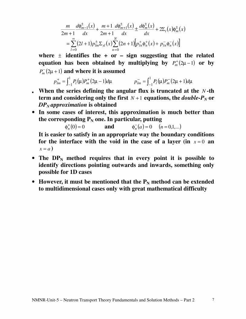
where ± identifies the + or – sign suggesting that the related
equation has been obtained by multiplying by ( )12 −µ+mP or by
( )12 +µ−mP and where it is assumed
( ) ( )∫−++ µ−µµ=
1
112 dPPp mllm ( ) ( )∫−
−− µ+µµ=1
112 dPPp mllm
• When the series defining the angular flux is truncated at the N -th
term and considering only the first 1+N equations, the double-PN or
DPN approximation is obtained
• In some cases of interest, this approximation is much better than
the corresponding PN one. In particular, putting
( ) 00 =φ+n and ( ) 0=φ−
an ( )...,1,0=n
It is easier to satisfy in an appropriate way the boundary conditions
for the interface with the void in the case of a layer (in 0=x an
ax = )
• The DPN method requires that in every point it is possible to
identify directions pointing outwards and inwards, something only
possible for 1D cases
• However, it must be mentioned that the PN method can be extended
to multidimensional cases only with great mathematical difficulty

NMNR-Unit-5 – Neutron Transport Theory Fundamentals and Solution Methods – Part 2 8
THE INTEGRAL EQUATION
FOR 1D AND 2D PROBLEMS 1D Geometry
• Considering an isolated slab included in the interval ax ≤≤0 with
isotropic scattering and indipendent source, in Cartesian
coordinates the transport equation in integral form
( )( )
( ) ( ) ( )∫ ∫ ′
′+′′′φ→′′Σ
′−π=φ
∞′τ−
V
s
Err
VdErSEdErEErrr
eEr ,,,
4, 00 02
,,
becomes
( )( )
( ) ( ) ( )∫ ∫ ′′′
′+′′′φ→′′Σ
′−π=φ
∞′τ−
V
s
Err
zdydxdExSEdExEExrr
eEx ,,,
4, 00 02
,,
or
( ) ( ) ( ) ( )( )
∫ ∫∫∫ ′′−π
′
′+′′′φ→′′Σ′=φ
∞
∞−
′τ−∞
∞−
∞aErr
s zdrr
eydExSEdExEExxdEx
0 2
,,
00 04
,,,,
where the integration along the coordinates other than x is isolated
at the right, to be made first as as afucntion of any x
• It is now convenient to change the integration variables, so that we
can take full profit of the 1D characteristics of the problem
• The reference frame is selected such that 0,0,xr =
zyxr ′′′=′ ,,
then introducing polar coordinates in the plane zy ′′ , with azimuth ϕ
and vector radius p 22
zyp ′+′=
0 ′x x a
′r
r
θ
0
y
x
z
′r
r
′x
ϕ
θp

NMNR-Unit-5 – Neutron Transport Theory Fundamentals and Solution Methods – Part 2 9
• It is therefore ( ) ( )
( )[ ] dpppxx
edzd
rr
eyd
ErrErr
∫∫∫∫∞
′τ−π∞
∞−
′τ−∞
∞− +′−πϕ=′
′−π′
0 22
,,2
02
,,
44
• Now it is therefore convenient to substitute to p the variable t
defined as:
( )xx
pxx
xx
rrt
′−
+′−=
′−
′−=
θ≡
22
cos
1
( )∞<≤ t1
obtaining
( ) ( ) 22222
1
rr
dpp
pxx
dpp
t
dt
pxx
dpp
xxdt
′−=
+′−=⇒
+′−′−=
and then
ϕ′−=ϕ dt
dtrrddpp
2
• We have therefore: ( ) ( )
( )[ ]( )
t
dtedpp
pxx
edzd
rr
eyd
tExxErrErr
∫∫∫∫∫∞ ′τ−∞
′τ−π∞
∞−
′τ−∞
∞−=
+′−πϕ=′
′−π′
1
,,
0 22
,,2
02
,,
2
1
44
where it can be noted that we used the “obvious” relation:
( ) ( ) ( )tExxExx
Err ,,cos
,,,, ′τ=
θ
′τ=′τ
In fact, we recognise that when the neutron trajectory is inclined
with respect to the x axis, this results just in an increase by a factor
θcos1 in the number of mean free paths involved in their flight
• So defining the exponential integral functions
( )n
tzn
t
dtezE ∫
∞ −=1
it is
( ) ( )[ ] ( ) ( ) ( )∫ ∫ ′
′+′′′φ→′′Σ′τ=φ
∞a
s xdExSEdExEExExxEEx0 00 01 ,,,,,
2
1,
• In the monokinetic case it is:
( ) ( )[ ] ( ) ( ) ( )[ ]∫ ′′+′φ′Σ′τ=φa
s xdxSxxxxEx0 001 ,
2
1
• When the layer [ ]a,0 is homogeneous (same material everywhere), it
is simply ( ) xxxx t ′−Σ=′τ , and therefore
( ) [ ] ( ) ( ) ( )[ ]∫ ′′+′φ′Σ′−Σ=φa
st xdxSxxxxEx0 001
2
1

NMNR-Unit-5 – Neutron Transport Theory Fundamentals and Solution Methods – Part 2 10
• If we choose the meen free path as length scale (i.e., substituting to
x the coordinate xtΣ=τ ) it is
( ) ( ) ( ) ( ) ( )[ ]∫Σ
τ′τ′+τ′φτ′Στ′−τΣ
=τφa
st
tdSE
0 0012
1
• This relation can be reached also for a non-homogeneous layer.
Putting:
( ) ( )∫ ′′′′Σ=τ→x
t xdxxx0
( )dxxd tΣ=τ
and, expressing the flux as a function of τ in place of x , it is
( ) ( ) ( ) ( ) ( )[ ]∫τ
τ′τ′+τ′φτ′τ′−τ=τφa
dscE0 01
2
1
where
t
scΣ
Σ= 0 and
t
Ss
Σ= 0
0
That is coincident with reation obtained in the case of a
homogenoeus layer by substituting atΣ with the more general form
( )dxxa
ta ∫ Σ=τ0
.
2D Geometry
• We consder a “geenralized cylinder” (not necessarily circular)
infinite in height and isolated having a volume V having as
intersection with the plane 0=z the general surface 0A
• We also assume that the scattering and the independent source are
isotropic
• If the variables in the problem depend only on x and y , the integral
transport equation becomes
( )( )
( ) ( ) ( )∫ ∫ ′′′
′′+′′′′φ→′′′Σ
′−π=φ
∞′τ−
V
s
Err
zdydxdEyxSEdEyxEEyxrr
eEyx ,,,,,,
4,, 00 02
,,
or
( ) ( ) ( ) ( )( )
∫ ∫∫ ′′−π
′′+′′′′φ→′′′Σ′′=φ
∞
∞−
′τ−∞
0
2
,,
00 04
,,,,,,,,
A
Err
s zdrr
eEyxSEdEyxEEyxydxdEyx
where we now isolated in the RHS the integration over z
• Therefore, also in the 2D case an appropriate choice of the
coordinate helps in obtaining a final compact form; it is:
0,,0 yxrr ≡=
and zyxr ′′′≡′ ,,
NMNR-Unit-5 – Neutron Transport Theory Fundamentals and Solution Methods – Part 2 11
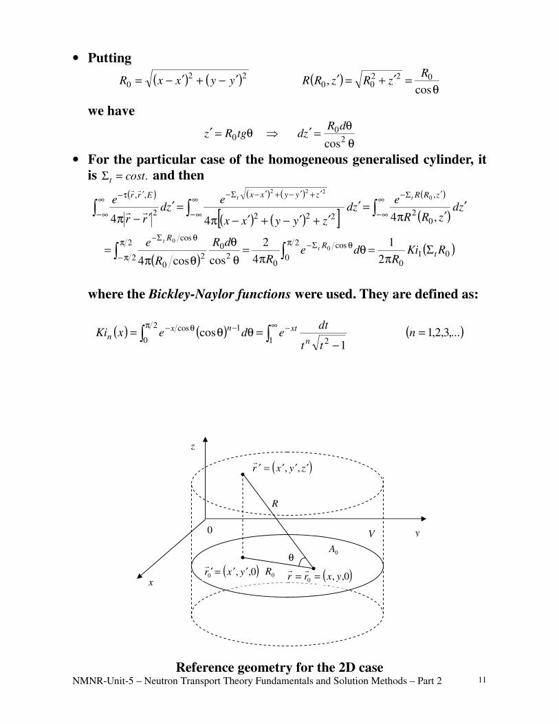
• Putting
( ) ( )220 yyxxR ′−+′−= ( )
θ=′+=′
cos, 022
00
RzRzRR
we have
θ
θ=′⇒θ=′
20
0cos
dRzdtgRz
• For the particular case of the homogeneous generalised cylinder, it
is .tsoct =Σ and then
( ) ( ) ( )
( ) ( )[ ]( )
( )zd
zRR
ezd
zyyxx
ezd
rr
ezRRzyyxxErr tt
′′π
=′′+′−+′−π
=′′−π
∫∫∫∞
∞−
′Σ−∞
∞−
′+′−+′−Σ−∞
∞−
′τ−
,444 02
,
2222
,, 0222
( )( )01
0
2
0
cos
02
02
2 20
cos
2
1
4
2
coscos4
0
0
RKiR
deR
dR
R
et
RR
t
t
Σπ
=θπ
=θ
θ
θπ= ∫∫
π θΣ−π
π−
θΣ−
where the Bickley-Naylor functions were used. They are defined as:
( ) ( ) ( )...,3,2,11
cos1 2
2
0
1cos =−
=θθ= ∫∫∞ −π −θ−
ntt
dtedexKi
n
xtnxn
Reference geometry for the 2D case
x
y
z
0
( )
r r x y= =0 0, ,( )
′ = ′ ′r x y0 0, ,
( )
′ = ′ ′ ′r x y z, ,
V
A0
R0
R
θ

NMNR-Unit-5 – Neutron Transport Theory Fundamentals and Solution Methods – Part 2 12
• In the general case in which the cylinder is non-homogeneous, it is
( ) ( )θ
′τ=′τ
cos
,,,, 00 ErrErr
and then ( ) ( )
( ) θ
θ′−
θ′−π=′
′−π∫∫
πθ′τ−
∞
∞−
′τ−
2
002
0 2
00
cos,,
2
,,
coscos2
1
4
00 drr
rr
ezd
rr
eErrErr
( ) ( )[ ]ErrKirr
derr
Err,,
2
1
2
1001
00
2
0
cos,,
00
00 ′τ′−π
=θ′−π
= ∫π θ′τ−
• It can be then concluded that
( ) ( )[ ] ( ) ( ) ( )∫ ∫ ′
′+′′′φ→′′Σ
′−π
′τ=φ
∞
0
0000 00000
0010 ,,,
2
,,,
A
s AdErSEdErEErrr
ErrKiEr
• In the particular case of a monokinetic problem
( ) ( )[ ] ( ) ( ) ( )[ ]∫ ′′+′φ′Σ′−π
′τ=φ
0
00000000
0010
2
,
A
s AdrSrrrr
rrKir
• Finally, if the cylinder is homogeneous
( )[ ]
( ) ( )[ ]∫ ′′+′φΣ′−π
′−Σ=φ
0
0000000
0010
2A
st
AdrSrrr
rrKir
FINAL CONSIDERATIONS
The above explains why in 1D and 2D codes based on the integral
equations, collision probabilities involve exponential integral functions
and Bickley-Naylor functions, respectively
As usual, we note that in reduced dimensionality problems we need
anyway to consider that neutrons travel in the 3D space, integrating
along the neglected dimensions in order to obtain the overall
contribution of neutron sources that are actually distributed in a 3D
space

NMNR-Unit-5 – Neutron Transport Theory Fundamentals and Solution Methods – Part 2 13
DISCRETE ORDINATE METHOD
OR “SN” METHOD
General considerations
• The discrete ordinate method is based on the solution of the
interodifferential equation discretised both in the space and in the
angular coordinates
• This method represents the main technique for the solution of the
integrodifferential transport equation since it allows to easily obtain
a solution with any degree of approximation as a function of the
available computational resources
• The first algorithms of these methods can be traced back to
methods adopted for stellar atmospheres; the technique was then
extended mainly owing to B. Carlson to nuclear energy applications
• The remarkable efficiency of these methods, named SN metods,
makes them to be often preferred to others
The one-dimensional case in cartesian coordinates
Discretised equations
• From the steady-state integro-differential equation
( ) ( ) ( ) ( ) ( ) ( )Ω+Ω′′Ω′′φΩ→Ω′′Σ=ΩφΣ+Ωφ⋅Ω ∫
vrSdvdvrvvrvrvrvrgrad str ,,,,,,
we can firstly consider (just for simplicity) the monokinetic case
with isotropic scattering
( ) ( ) ( ) ( ) ( ) ( )Ω+Ω′Ω′φπ
Σ=ΩφΣ+Ωφ⋅Ω ∫
,,4
,, rSdrr
rrrgrad str
and we finally consider the already obtained form for 1D geometry ( ) ( ) ( )
( )( ) ( )µ+µ′µ′φ
Σ=µφΣ+
∂
µφ∂µ ∫− ,,
2,
, 1
1xSdx
xxx
x
x st (°)
• In order to solve this equation, we define M discrete directions and
corresponding weighting coefficients
Mµµµ ...,,, 21 Mwww ...,,, 21
• In particular, making use of the weighting coefficients mw
(quadrature coefficients) it is possible to calculate in an
approxomated way the integral at RHS of (°), that is:
( ) ( )∑∫=
−µφ≈µ′µ′φ
M
m
mm xwdx1
1
1,,

NMNR-Unit-5 – Neutron Transport Theory Fundamentals and Solution Methods – Part 2 14
• Owing to this discretisation of the angular coordinate Eq. (°) is
transformed into the following
( )( ) ( )
( )( ) ( )m
M
n
nns
mtm
m xSxwx
xxx
xµ+µφ
Σ=µφΣ+
∂
µφ∂µ ∑
=
,,2
,,
1
( )m M= 1, ...,
• The choice of the weighting coefficients mw and, then of the
quadrature formulations is generally made with reference to an
even number of discrete ordinates mµ chosen in a symmetric way
with respect to 0=µ
• It is, therefore:
mmMm µ−=µ>µ −+10
==−+
2...,,2,11
Mmww mmM
• The reason of the choice of symmetrically distributed values with
respect to 0=µ with equal weights is due to the intent to assign the
same importance to particles streaming along different directions
• The even number of directions is then adopted in order to avoid the
existence of a value of m such that 0=µm ; this would pose
problems, since:
♦ the derivative term would disappear in the equation, compelling to
treat this direction in a different way with respect to the others
♦ as already noted, the direction characterised by 0=µ can be the
one at which discontinuities may appear in flux along the angular
coordinate
• The advantage to choose an even number of discrete ordinates also
appears in particular when boundary conditions are imposed:
♦ in the case of pure reflection, for instance at 0=x , it is:
( ) ( )
=µφ=µφ −+
2...,,2,1,0,0 1
MmmMm
♦ for a free surface (interface to the void) in ax = , instead, it is:
( )
+==µφ M
Mma m ...,,1
20,
• In principle, there is anyway a considerable freedom in determining
the directions
• A very frequent choice is the one (of Wick-Chandrasekhar) in which
the mµ are assigned such that they are the M zeroes of the Legendre
polynomial of order M : ( ) ( )MmP mM ...,,2,10 ==µ

NMNR-Unit-5 – Neutron Transport Theory Fundamentals and Solution Methods – Part 2 15
• Its is moreover requested that ( )Mmwm ...,,2,10 =>
and that the weighting is such to provide an exact integration over
11 ≤µ≤− of all the polynomials of order up to 1−M ; it is therefore:
∑ ∫=
−
+=µµ=µ
M
m
nnmm
disparin
parinn
dw1
1
1
0
,1
2
( )1...,,2,1,0 −= Mn
• It is necessary to note that the previous relationships with odd n is
identically satisfied for any set of mµ and mw respecting the
requirements
mmMm µ−=µ>µ −+10
==−+
2...,,2,11
Mmww mmM
• Therefore it is possible to determine the M independent parameters
mµ and mw ( )2...,,1 Mm = in order to exactly integrate all the
polynomials having order 22...,,2,0 −M (and also those of order
12 −M , since that this is and odd number)
• We have therefore:
( ) ( ) ( ) ( ) ( )1...,,1,0,12
21
11
−=+
δ=µµµ=µµ ∫∑ −
=
Mlkk
dPPPPw kllk
M
m
mlmkm
( ) ( ) ( ) ( )φ µ φ µ φ µ φ µ0 0 0 01 4 2 3, , ; , ,= = ( ) ( )φ µ φ µa a, ,3 4 0= =
Pure reflection Free surface
Discrete ordinate in the planarcase and boundary conditions ( )4=M
x
2µ
1µ4µ
3µ
a 0
µ = 0
2µ
1µ4µ
3µ
0
µ = 0
µ = −1 µ = 1 µ = −1 µ = 1

NMNR-Unit-5 – Neutron Transport Theory Fundamentals and Solution Methods – Part 2 16
• With these requirements µm and wm are given by the Gauss-
Legendre quadrature parameters reported in the above table for 6,4,2=M
• It is possible to show that, with this choice, the method is equivalent
to the on of spherical harmonics NP , with 1−= MN :
1−≡ MM PS
• The numerical solution is obtained by writing the equations in the
form ( )
( ) ( ) ( )mmtm
m xqxxx
xµ=µφΣ+
∂
µφ∂µ ,,
, ( )Mm ...,,1=
and iterating on the scattering source by the scheme: [ ]( )
( ) [ ]( ) [ ]( )mt
mt
tm
t
m xqxxx
xµ=µφΣ+
∂
µφ∂µ +
+
,,, 1
1
( )Mm ...,,1=
[ ]( )( ) [ ]( ) ( )m
M
n
nt
ns
mt
xSxwx
xq µ+µφΣ
=µ ∑=
++,,
2,
1
11
• It is obviously needed also a spatial discretisation:
♦ the interval ax ≤≤0 is subdivided into I subintervals with
uniform properties
2=N 000.121 == ww 57735.021 =µ−=µ
4=N 65215.032 == ww 33998.032 =µ−=µ
34785.041 == ww 86114.041 =µ−=µ
6=N 46791.043 == ww 23862.043 =µ−=µ
36076.052 == ww 66121.052 =µ−=µ
17132.061 == ww 93247.061 =µ−=µ
Gauss-Legendre quadrature parameters (from Bell & Glasstone, 1979)
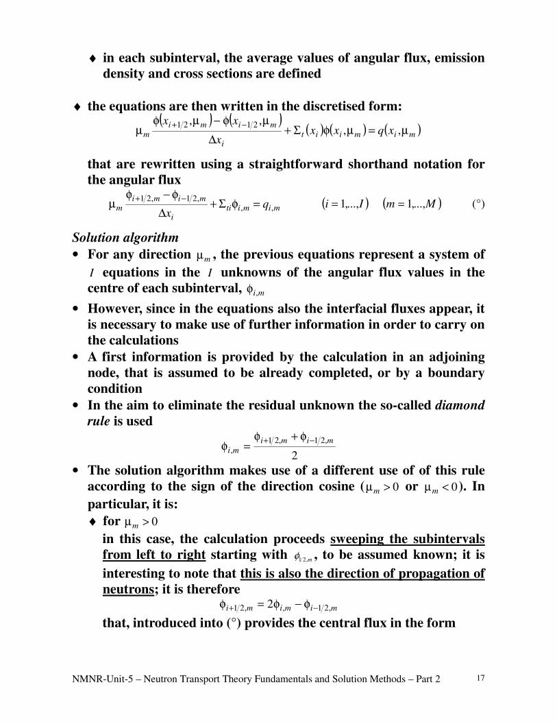
Spatial discretisation for the discrete ordinate method
0>µ
x x1 2
x1 x3 xi
xi−1xi+1 x I −1
x I x3 2
x5 2 xi−1 2 xi+1 2
x I −1 2 x I +1 2
ix∆ 0<µ
NMNR-Unit-5 – Neutron Transport Theory Fundamentals and Solution Methods – Part 2 17
♦ in each subinterval, the average values of angular flux, emission
density and cross sections are defined
♦ the equations are then written in the discretised form: ( ) ( )
( ) ( ) ( )mimiiti
mimi
m xqxxx
xxµ=µφΣ+
∆
µφ−µφµ
−+,,
,, 2121
that are rewritten using a straightforward shorthand notation for
the angular flux
mimitii
mimim q
x,,
,21,21=φΣ+
∆
φ−φµ
−+ ( )Ii ...,,1= ( )Mm ...,,1= (°)
Solution algorithm
• For any direction mµ , the previous equations represent a system of
I equations in the I unknowns of the angular flux values in the
centre of each subinterval, mi,φ
• However, since in the equations also the interfacial fluxes appear, it
is necessary to make use of further information in order to carry on
the calculations
• A first information is provided by the calculation in an adjoining
node, that is assumed to be already completed, or by a boundary
condition
• In the aim to eliminate the residual unknown the so-called diamond
rule is used
2
,21,21
,
mimi
mi
−+ φ+φ=φ
• The solution algorithm makes use of a different use of of this rule
according to the sign of the direction cosine ( 0>µm or 0<µm ). In
particular, it is:
♦ for 0>µm
in this case, the calculation proceeds sweeping the subintervals
from left to right starting with φ1 2,m , to be assumed known; it is
interesting to note that this is also the direction of propagation of
neutrons; it is therefore
mimimi ,21,,21 2 −+ φ−φ=φ
that, introduced into (°) provides the central flux in the form

NMNR-Unit-5 – Neutron Transport Theory Fundamentals and Solution Methods – Part 2 18
tim
mim
mi
mi x
qx
Σµ
∆+
µ
∆+φ
=φ−
21
2,,21
, (°°)
once the central flux is known, it is therefore possible to evaluate
the interfacial flux mimimi ,21,,21 2 −+ φ−φ=φ to be used in the
calculation of the next subinterval;
♦ for 0<µm
unlike in the case 0>µm , the calculation proceeds from right to
left; it is again worth to note that this is also the direction of
propagation of neutrons (now it is, in fact, 0cos <θ=µ mm ); we put
therefore:
mimimi ,21,,21 2 +− φ−φ=φ
that, introduced into (°) allows to obtain the central flux in the
form:
tim
mim
mi
mi x
qx
Σµ
∆+
µ
∆+φ
=φ
+
21
2,,21
,
once the central flux is known, it is therefore possible to evaluate
the interfacial flux mimimi ,21,,21 2 +− φ−φ=φ to be used in the
calculation of the next subinterval.
• The order of accuracy obtained by the diamond rule can be
analysed considering the particular case of zero emission density
and constant total cross section ( )
( ) 0,,
=µφΣ+µφ
µ mtm
m xxd
xd
whose exact solution is
( ) ( ) ( ) mt xxmm exx
µ′−Σ−µ′φ=µφ /,,
In particular, putting 21−=′ ixx and 21+= ixx it is h
mimi e−
−+ φ=φ ,21,21
where
m
t xh
µ
∆Σ=

NMNR-Unit-5 – Neutron Transport Theory Fundamentals and Solution Methods – Part 2 19
Making use of the relations
tim
mim
mi
mi x
qx
Σµ
∆+
µ
∆+φ
=φ−
21
2,,21
, and mimimi ,21,,21 2 −+ φ−φ=φ
it is finally found 21
21,21,21
h
hmimi
+
−φ=φ −+
to be considered in view that ( )3
21
21hO
h
he
h ++
−=−
• Notwithstanding the high accuracy of the method, considering the
above relationship it can be noted that when 2>h it is 021 <φ +i even
if 021 >φ −i
• It is a typical problem of this method encountered during
calculation advancement that occurs when the relationships
mimimi ,21,,21 2 −+ φ−φ=φ 0>µm
mimimi ,21,,21 2 +− φ−φ=φ 0<µm
provide negative values of the interface flux
• The problem can be solved by using a finer spatial discretisation, in
order to get 2<h ; however, this is not always convenient, e.g. in the
case of strongly absorbing regions and/or very much inclined
direactions
• However, it is possible to correct (“fix”) the flux making use of one
of two simple rules for “fix-up”
♦ 1st RULE (“step method”)
for 0>µm whenever it is 02 ,21,,21 <φ−φ=φ −+ mimimi , it is assumed
mimi ,,21 φ=φ + (instead of the diamond rule), then calculating mi,φ as
a consequence of this choice by (°); similarly in case of 0<µm ,…
(just exchange the role of the two interfaces);
♦ 2nd RULE (“set offending flux to zero and recompute”)
for 0>µm whenever it is 02 ,21,,21 <φ−φ=φ −+ mimimi , it is assumed
0,21 =φ + mi (instead of the diamond rule), then calculating mi,φ as a
consequence of this choice by (°);similarly in case of 0<µm , …
(just exchange the role of the two interfaces).
• Unfortunately the use of these rules decreases the accuracy of the
method from the second order to the first one

NMNR-Unit-5 – Neutron Transport Theory Fundamentals and Solution Methods – Part 2 20
• Let us just note that the assumption of an isotrpic scattering source
is not at all needed for the application of the above describe
algorithm; on the contrary, discrete ordinates methods are
particularly suitable for dealing with scattering anisotropy
• In fact, when the anisotrpy of scattering in the laboratory reference
frame is up to the order L , making use of the expansion in
Legendre polynomials, we have
( ) ( ) ( ) ( ) ( ) ( ) ( )µ+φµΣ+
=µφΣ+∂
µφ∂µ ∑
=
,2
12,
,
0
xSxPxl
xxx
x L
l
llslt
with ( ) ( ) ( )∫− µ′µ′φµ′=φ1
1, dxPx ll
• The discrete ordinate form of this equation is therefore given by
( )( ) ( ) ( ) ( ) ( ) ( )m
L
l
lmlslmtm
m xSxPxl
xxx
xµ+φµΣ
+=µφΣ+
∂
µφ∂µ ∑
=
,2
12,
,
0
( )Mm ...,,1=
( ) ( ) ( )∑=
µφµ=φM
n
nnlnl xPwx0
,
• On the basis of this relationship, it is then possible to set up a
solution algorithm quite similar to the one just described for the
case of the isotropic scattering
The one-dimensional case in spherical coordinates
Form of the transport equation
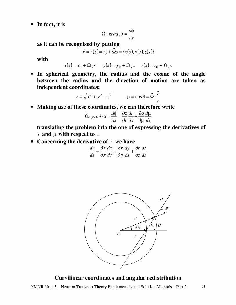
• In the figure reported in the next page, an unfortunate feature of
the transport equation in curvilinear coordinates is described; it
consists in the fact that the angular coordinate identifying the
direction of neutrons changes during the rectilinear motion of
neutron
• As a consequence of this phenomenon, known as angular
redistribution, the “streaming” term of the integro-differential
equation involves derivatives in the angular coordinate
• In order to obtain the streaming term in spherical coordinates, it is
necessary to remember that it represents a differentiation along the
direction of motion of neutrons
NMNR-Unit-5 – Neutron Transport Theory Fundamentals and Solution Methods – Part 2 21
• In fact, it is
ds
dgradr
φ=φ⋅Ω
as it can be recognised by putting
( ) ( ) ( ) ( ) szsysxsrsrr ,,0 ≡Ω+==
with ( ) sxsx xΩ+= 0 ( ) sysy yΩ+= 0 ( ) szsz zΩ+= 0
• In spherical geometry, the radius and the cosine of the angle
between the radius and the direction of motion are taken as
independent coordinates:
222zyxr ++≡
r
r
⋅Ω=θ≡µ cos
• Making use of these coordinates, we can therefore write
ds
d
ds
dr
rds
dgradr
µ
∂µ
∂φ+
∂
∂φ=
φ=φ⋅Ω
translating the problem into the one of expressing the derivatives of
r and µ with respect to s
• Concerning the derivative of r we have
ds
dz
z
r
ds
dy
y
r
ds
dx
x
r
ds
dr
∂
∂+
∂
∂+
∂
∂=
Curvilinear coordinates and angular redistribution
′θ
θ
r
Ω
∆θ
′r
0
NMNR-Unit-5 – Neutron Transport Theory Fundamentals and Solution Methods – Part 2 22
• Since making use of the previous definitions it is
r
x
x
r=
∂
∂
r
y
y
r=
∂
∂
r
z
z
r=
∂
∂
and
xds
dxΩ= y
ds
dyΩ= z
ds
dzΩ=
it is
µ=⋅Ω=Ω+Ω+Ω=r
r
r
z
r
y
r
x
ds
drzyx
• Similarly, for the derivative with respect to µ we have:
∂
∂+
∂
∂+
∂
∂⋅Ω−
++⋅Ω
=
⋅Ω=
µ
ds
dz
z
r
ds
dy
y
r
ds
dx
x
r
r
rk
ds
dzj
ds
dyi
ds
dx
rr
r
ds
d
ds
d2
Ω+Ω+Ω
⋅Ω−Ω+Ω+Ω⋅
Ω= zyxzyx
r
z
r
y
r
x
r
rkji
r 2
( )rr
r
rr
r
r
22
3
21
111 µ−
=
⋅Ω−=
⋅Ω−=
• The transport equation in spherical coordinates for the monokinetic
case and isotropic scattering becomes therefore
( ) ( ) ( ) ( )( )
( ) ( )µ+µ′µ′φΣ
=µφΣ+∂µ
µ∂φµ−+
∂
µ∂φµ ∫− ,,
2,
,1, 1
1
2
rSdrr
rrr
rr
r st
• In view of the spatial and angular discretisation, it is convenient to
recast the streaming term into a conservative form, i.e., in a form
that allows integration over a finite volume of the coordinates with
“exact” neutron conservation
• In spherical geometry, the control volumes on which we need to
integrate are spherical shells; by integrating the streaming term
over the general shell with inner and outer radiuses 1r and 2r and
over all directions, we have:
( ) µφππφ ddrrdVdgradr
rr ∫∫∫ ∫ −
Ω⋅∇=Ω⋅Ω1
1
2 242
1
( ) ( ) ( )1
2
12
2
2
2 4442
1
rJrrJrdrrJrr
rπππ −=⋅∇= ∫
• In order to make this result be obtained easily after multiplication
by 24 rπ , the streaming term is rewritten as
( ) ( )[ ]
µ∂
∂φµ−+
∂
∂φµ=
µ∂
∂φµ−+µφ−µφ+
∂
∂φµ=φµ−
∂µ
∂+φ
∂
∂µ
rrrrrrrr
rr
2222
2
11221
1

NMNR-Unit-5 – Neutron Transport Theory Fundamentals and Solution Methods – Part 2 23
It is
( ) ( )[ ]∫∫ −µ
φµ−∂µ
∂+φ
∂
∂µππ
1
1
22
2
2 11
242
1
dr
rrr
drrr
r
( )[ ]
0
1
1
221
1
21824
2
1
2
2
1
=
−−µφµ−
∂µ
∂π+
µφµπ
∂
∂π= ∫∫∫∫ ddrrdrdr
r
r
r
Jr
r
r
( ) ( ) ( )[ ]12
122
22 44
2
1
rJrrJrdrJrr
r
r−π=
∂
∂π= ∫
• The conservative form of the transport equation in spherical
coordinates is therefore:
( ) ( )[ ] ( ) ( )( )
( ) ( )µ+µ′µ′φΣ
=µφΣ+φµ−∂µ
∂+φ
∂
∂µ∫− ,,
2,1
1 1
1
22
2rSdr
rrr
rr
rr
st
• Finally, introducing the emission density
( )( )
( ) ( )µ+µ′µ′φΣ
=µ ∫− ,,2
,1
1rSdr
rrq s
we have
( ) ( )[ ] ( ) ( ) ( )µ=µφΣ+φµ−∂µ
∂+φ
∂
∂µ,,1
1 22
2rqrr
rr
rrt (°)
Discretised equations
• In similarity with the Cartesian plane case, also in spherical
geometry there is no variation of the angular flux with the angle ϕ
• Therefore, the angular discretisation affects only µ
• The spatial discretisation is made in similarity with what already
observed for the plane case in Cartesian coordinates
• The rectangular discretisation domain shown in the Figure at the
bottom of this page is so obtained, where the “diamond”, giving the
name to the already mentioned rule, is clearly shown
• By integrating (°) on this domain and in ϕd over π<ϕ< 20 , it is:
( ) ( )[ ]04
1121
21
21
21
222
2
2
0=π
−φΣ+µ∂
φµ−∂+
∂
φ∂µµϕ ∫∫∫
+
−
+
−
µ
µ
π i
i
m
m
r
r t drrqrr
r
rdd
from which we have
( ) ( )[ ] µµφπ−µφπµπ −−++
µ
µ∫+
−
drrrr iiiim
m
,4,42 212
21212
2121
21
( ) ( ) ( ) ( )[ ]∫+
−−−++ µφµ−−µφµ−π+
21
2121
22121
221
2,1,18
i
i
r
r mmmm drrrr
( ) 04221
21
21
21
2 =π−φΣµπ+ ∫∫+
−
+
−
µ
µ
i
i
m
m
r
r t drrqd

NMNR-Unit-5 – Neutron Transport Theory Fundamentals and Solution Methods – Part 2 24
• It can be noted that the use of the conservative form of the
transport equation allowed a quite easy integration
• The three obtained integral terms are then approximated. For the
first term, it is
( ) ( )[ ] µµφπ−µφπµπ −−++
µ
µ∫+
−
drrrr iiiim
m
,4,42 212
21212
2121
21 ( )miimiimm AAw ,2121,21214 −−++ φ−φµπ≅
where we assumed
( )21212
1−+ µ−µ= mmmw ( )2121
2
1−+ µ+µ=µ mmm 2
2121 4 ±± π= ii rA
and mi ,21±φ represents the mean angular flux on the angular element
mm wπ4=∆Ω holding fot the two surfaces at the radiuses 21−ir or 21+ir :
( )∫∫+
−
µ
µ ±
π
± µµφϕπ
=φ21
21
,4
121
2
0,21m
m
drdw
im
mi
• The second term is now approximated as:
( ) ( ) ( ) ( )[ ]∫+
−−−++ µφµ−−µφµ−π
21
2121
22121
221
2,1,18
i
i
r
r mmmm drrrr
( )21,2121,214 −−++ φ−φπ≈ mimmim aa
where 21, ±φ mi is the mean flux over the volume iV (spherical shell
between 21−ir and
21+ir ), corresponding to 21−µ
i and
21+µi
( )∫+
−
πµφ=φ ±±21
21
22121, 4,
1 i
i
r
r mi
mi drrrV
( )321
321
3
4−+ −π= iii rrV
while the constants 21−ma e 21+ma represent the effect of anfular
redistribution, whose value will be described later
• The third integral is finally approximated as :
Angular and space discretisation in spherical geometry
µ
r
µm+1 2
µm
µm−1 2
ri−1 2 ri+1 2ri

NMNR-Unit-5 – Neutron Transport Theory Fundamentals and Solution Methods – Part 2 25
( ) ( )imimtiim
r
r t qVwdrrqdi
i
m
m
−φΣπ≅π−φΣµπ ∫∫+
−
+
−
µ
µ442
21
21
21
21
2
where imφ and imq represent mean values of the angular flux and of
the emission density over m∆Ω and iV in the spherical shell
( )∫ ∫ ∫π µ
µ
+
−
+
−
πµφµϕπ
=φ2
0
221
21
21
21
4,4
1 m
m
i
i
r
rim
im drrrddVw
( )∫ ∫ ∫π µ
µ
+
−
+
−
πµµϕπ
=2
0
221
21
21
21
4,4
1 m
m
i
i
r
rim
im drrrqddVw
q
• Adopting the above approximations, the discretised neutron
transport equation in 1D spherical geometry takes the form
( )miimiim AA ,2121,2121 −−++ φ−φµ ( )21,2121,21
1−−++ φ−φ+ mimmim
m
aaw
( ) 0=−φΣ+ imimtii qV
• In order to obtain the angular discretisation coefficients, one
proceeds as follows:
♦ it is noted that for uniform and istropic flux it is
mimimi ,,21,21 φ=φ=φ −+
requiring that streaming term is zero, so that
imimti q=φΣ ;
then, it must be requested that
( ) 21212121 +−−+ −=−µ mmiimm aaAAw (*)
♦ however, in the general case the term depending on the angular
derivative must become zero when integrated over all the
directions; therefore, since it must be
( ) 021,2121,211
21,2121,21 =φ−φ=φ−φ ++=
−−++∑ iMiM
M
m
mimmim aaaa ;
since 21,iφ and 21, +φ Mi are arbitrary, it must be also
02121 == +Maa
• So, assuming 021 =a the equation (*) allows to calculate all the
coefficients ma by recurrence.
Solution algorithm
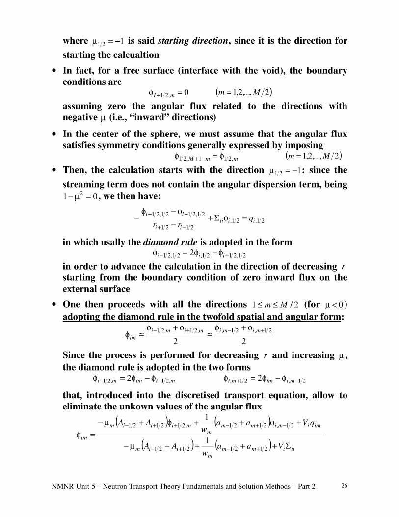
• The directions are chosen so that
1...0...1 212112212223121 =µ<µ<µ<<µ<=µ<µ<<µ<µ<µ=− +−++ MMMMMM
NMNR-Unit-5 – Neutron Transport Theory Fundamentals and Solution Methods – Part 2 26
where 121 −=µ is said starting direction, since it is the direction for
starting the calcualtion
• In fact, for a free surface (interface with the void), the boundary
conditions are ( )2,...,2,10,21 MmmI ==φ +
assuming zero the angular flux related to the directions with
negative µ (i.e., “inward” directions)
• In the center of the sphere, we must assume that the angular flux
satisfies symmetry conditions generally expressed by imposing ( )2,...,2,1,211,21 MmmmM =φ=φ −+
• Then, the calculation starts with the direction 121 −=µ : since the
streaming term does not contain the angular dispersion term, being
012 =µ− , we then have:
21,21,2121
21,2121,21iiti
ii
iiq
rr=φΣ+
−
φ−φ−
−+
−+
in which usally the diamond rule is adopted in the form
21,2121,21,21 2 +− φ−φ=φ iii
in order to advance the calculation in the direction of decreasing r
starting from the boundary condition of zero inward flux on the
external surface
• One then proceeds with all the directions 2/1 Mm ≤≤ (for 0<µ )
adopting the diamond rule in the twofold spatial and angular form:
22
21,21,,21,21 +−+− φ+φ≅
φ+φ≅φ
mimimimi
im
Since the process is performed for decreasing r and increasing µ ,
the diamond rule is adopted in the two forms
miimmi ,21,21 2 +− φ−φ=φ 21,21, 2 −+ φ−φ=φ miimmi
that, introduced into the discretised transport equation, allow to
eliminate the unkown values of the angular flux
( ) ( )
( ) ( ) tiimmm
iim
imimimmm
miiim
im
Vaaw
AA
qVaaw
AA
Σ++++µ−
+φ++φ+µ−
=φ
+−+−
−+−++−
21212121
21,2121,212121
1
1

NMNR-Unit-5 – Neutron Transport Theory Fundamentals and Solution Methods – Part 2 27
where use is made of the definition of the angular differentiation
coefficients
• Once the values of the angular flux for all the directions with 0<µ
are computed, the following symmetry condition is used ( )2,...,2,1,211,21 MmmmM =φ=φ −+
in order to assigne the flux in the centre of the sphere for the
directions with 0>µ . The calculations then proceeds for increasing
r and µ , making use of the diamond rule in the two forms
miimmi ,21,21 2 −+ φ−φ=φ 21,21, 2 −+ φ−φ=φ miimmi
• Even in the spherical case, it is possible to encounter problems
related to the negative fluxes requiring the use of “fix-up” rules
• In some cases a non completely correct behaviour of the flux in the
centre of the sphere has be noted, to be attributed to a non-uniform
distribution of truncation erroras a function of r
• The condition ( )2,...,2,1,211,21 MmmmM =φ=φ −+
has been also considered criticisable, preferring sometimes the
relationship
00
=∂µ
∂φ
→r
discretised imposing that the angular flux at the centre of the
sphere is equal in all the directions
Sample advancement scheme for an S8 method with 10 radial nodes
r
µ
0
increasing µ
decreasing r
increasing µ
increasing r
Starting direction Zero angular flux
Symmetric angular flux

NMNR-Unit-5 – Neutron Transport Theory Fundamentals and Solution Methods – Part 2 28
The multidimensional case in Cartesian coordinates
Discretised equations
• In the multidimensional cases it is convenient to write the integro-
differential equation in the form
( )[ ] ( ) ( ) ( ) 0,,, =Ω−ΩφΣ+ΩφΩ
rqrrrdiv t
where again the following relationship has been used
( ) ( )[ ]ΩφΩ=Ωφ⋅Ω
,, rdivrgradr
• Considering a volume around the location kjiijk zyxr ,,=
, it is
kjiijk zyxV ∆∆∆= i
ijkkjjkijki
x
VzyAA
∆=∆∆== +− ,21,21
j
ijkkikjikji
y
VzxAA
∆=∆∆== +− ,21,,21,
k
ijkjikijkij
z
VyxAA
∆=∆∆== +− 21,21,
( ) ( ) ( )i I j J k K= = =1 1 1,..., ; ,..., ; ,...,
• To the general direction, mΩ
, the solid angle mm wπ=∆Ω 4 is then
assigned. We then define the average values of the flux over the
solid angle and the volume and also on the volume faces
∫ ∫π
φΩπ
=φ
m ijkw Vijkmmijk dVd
Vw4
,4
1 ∫ ∫
π±±
±
φΩπ
=φ
m jkiw Ajkimmjki dAd
Aw4,21
,,21
,21
4
1
∫ ∫π±
±
±
φΩπ
=φ
m kjiw Akjimmkji dAd
Aw4,21,
,,21,
,21,
4
1 ∫ ∫
π±±
±
φΩπ
=φ
m kijw Akijmmkij dAd
Aw421,
,21,
21,
4
1
• By integrating the transport equation over the solid angle
mm wπ=∆Ω 4 and over ijkV we have:
Reference frame and elementary volume
Ωm
dΩ ζm
µm
ηm0
y
z
x
∆xi
∆y j
∆zk
Ai jk−1 2,
Ai jk+1 2,
Ai j k, ,−1 2
Ai j k, ,+1 2
Aij k, +1 2
Aij k, −1 2
Vijk

NMNR-Unit-5 – Neutron Transport Theory Fundamentals and Solution Methods – Part 2 29
( )[ ] ( ) ( ) ( ) 0,,,
4
=
Ω−ΩφΣ+ΩφΩΩ∫ ∫
π m ijkw V
t dVrqrrrdivd
• The first term in this equation can be approximated as follows:
( )[ ] ( )[ ] ( ) ( )∫ ∫∫ ∫∫ ∫π ∂ππ
Ωφ⋅ΩΩ=ΩφΩΩ≅ΩφΩΩ
m ijkm ijkm ijk w V
mem
w V
mm
w V
dAruddVrdivddVrdivd
444
,,,
• Then, putting
mmm ζηµ≡Ω ,,
we have
( ) ( ) ( ) mjkijkimjkijkimm
w V
mem AAwdArud
m ijk
,21,21,21,21
4
4, −−++
π ∂
φ−φµπ≅Ωφ⋅ΩΩ∫ ∫
( ) ( )mijkkijmijkkijmmkijkjimkijkjim AAAA ,2121,,2121,,21,21,,21,21. −−++−−++ φ−φζ+φ−φη+
• Considering the previous definitions, it is:
( ) ( )
∆
φ−φµπ≅Ωφ⋅ΩΩ
−+
π ∂∫ ∫
i
mjkimjki
mijkm
w V
memx
VwdArud
m ijk
,21,21
4
4,
∆
φ−φζ+
∆
φ−φη+
−+−+
k
mijkmijk
mj
mkjimkji
mzy
,21,21,21,,21,
• It is also put
( ) ( ) ( ) ( )mijkmijkijktijkm
w V
t qVwdVrqrrd
m ijk
,,,
4
4,, −φΣπ≅Ω−ΩφΣΩ∫ ∫π
where it is
( )∫ ∫π
ΩΩπ
=
m ijkw Vijkmmijk dVrqd
Vwq
4
, ,4
1
• We finally have
i
mjkimjki
mx∆
φ−φµ
−+ ,21,21
k
mijkmijk
mj
mkjimkji
mzy ∆
φ−φζ+
∆
φ−φη+
−+−+ ,21,21,21,,21,
mijkmijkijkt q ,,, =φΣ+ ( ) ( ) ( ) ( )mNmKkJjIi ...,,1;...,,1;...,,1;...,,1 ====
representing the discrete ordinate form of the transport equation
for the multi-dimensional case
Solution algorithm and choice of directions
• Also in this case the solution algorithm takes into account the
direction of motion of neutrons and then of the sign of direction
cosines mµ , mη and mζ of mΩ
NMNR-Unit-5 – Neutron Transport Theory Fundamentals and Solution Methods – Part 2 30
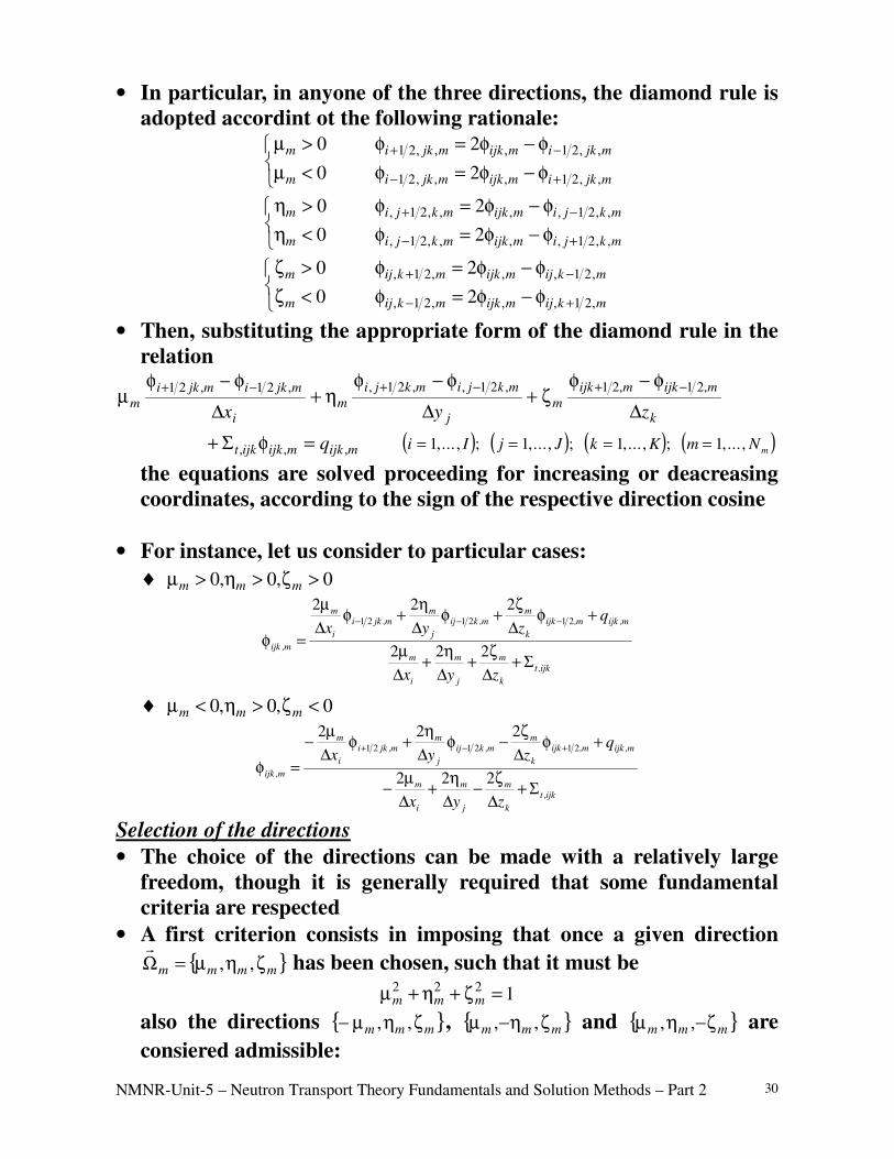
• In particular, in anyone of the three directions, the diamond rule is
adopted accordint ot the following rationale:
φ−φ=φ<µ
φ−φ=φ>µ
+−
−+
mjkimijkmjkim
mjkimijkmjkim
,,21,,,21
,,21,,,21
20
20
φ−φ=φ<η
φ−φ=φ>η
+−
−+
mkjimijkmkjim
mkjimijkmkjim
,,21,,,,21,
,,21,,,,21,
20
20
φ−φ=φ<ζ
φ−φ=φ>ζ
+−
−+
mkijmijkmkijm
mkijmijkmkijm
,21,,,21,
,21,,,21,
20
20
• Then, substituting the appropriate form of the diamond rule in the
relation
i
mjkimjki
mx∆
φ−φµ
−+ ,21,21
k
mijkmijk
mj
mkjimkji
mzy ∆
φ−φζ+
∆
φ−φη+
−+−+ ,21,21,21,,21,
mijkmijkijkt q ,,, =φΣ+ ( ) ( ) ( ) ( )i I j J k K m Nm= = = =1 1 1 1,..., ; ,..., ; ,..., ; ,...,
the equations are solved proceeding for increasing or deacreasing
coordinates, according to the sign of the respective direction cosine
• For instance, let us consider to particular cases:
♦ 0,0,0 >ζ>η>µ mmm
ijk,t
k
m
j
m
i
m
m,ijkm,ijk
k
mm,kij
j
mm,jki
i
m
m,ijk
zyx
qzyx
Σ+∆
ζ+
∆
η+
∆
µ
+φ∆
ζ+φ
∆
η+φ
∆
µ
=φ
−−−
222
222212121
♦ 0,0,0 <ζ>η<µ mmm
ijk,t
k
m
j
m
i
m
m,ijkm,ijk
k
mm,kij
j
mm,jki
i
m
m,ijk
zyx
qzyx
Σ+∆
ζ−
∆
η+
∆
µ−
+φ∆
ζ−φ
∆
η+φ
∆
µ−
=φ
+−+
222
222212121
Selection of the directions
• The choice of the directions can be made with a relatively large
freedom, though it is generally required that some fundamental
criteria are respected
• A first criterion consists in imposing that once a given direction
mmmm ζηµ=Ω ,,
has been chosen, such that it must be
1222 =ζ+η+µ mmm
also the directions mmm ζηµ− ,, , mmm ζη−µ ,, and mmm ζ−ηµ ,, are
consiered admissible:

NMNR-Unit-5 – Neutron Transport Theory Fundamentals and Solution Methods – Part 2 31
this allows imposing in a simple and direct way reflective conditions
orthogonal to the there axes of the reference frame
• Whenever such choice is made, it is possible to consider only the
directions included in a single octant, then translating the results to
the others
• A particularly interesting choice is the one consisting in imposing
that the adimissible directions are invariant to 90° rotation around
any axis of the reference frame
• These “level symmetric quadratures” are characterisedby the fact of
being selected making use of asingle degree of freedom. In fact, it is
assumed that the direction cosines are all chosen by a single set,
defined as 1...0...1 2/112/ <<<<<−<<−<− MM tttt
• Now, let us assume that we select three cosines such that
kmjmim ttt =ζ=η=µ
In this case, it must be obviously
1222 =++ kji ttt (a)
So, making the further choice im t=µ and 1+=η jm t , in order to
satisfy the normalisation relationships we require that 1−=ζ km t :
121
21
2 =++ −+ kji ttt (b)
By subtracting side by side (b) to (a) we get 2
1222
1 −+ −=− kkjj tttt
Since j and k are arbitrary, we have:
( )CittCtt iii 121
221
2 −+=⇒+= −
Finally, since it must be
122/
21
21 =++ Mttt
we finally get
( )2
312 21
−
−=
M
tC
• Since such quadratures involve for each axis 2M positive and 2M
negative values for each direction cosine, they are considered “SM
quadratures” (actually the general name is “SN”)
• The total number of directions per each octant is ( ) 8/2+MM and
the overall number on the unity radius sphere is ( )2+MM

NMNR-Unit-5 – Neutron Transport Theory Fundamentals and Solution Methods – Part 2 32
• For the weighting coefficients, a normalization on each octant is
generally adopted ( )
∑+
=
=8/2
1
1MM
m
Imw
where Imw = is the weighting coefficient for a general direction
related to the first octant
• As a consequence the scalar flux in ijkr
can be obtained by the
angular flux by the relationship ( )
∑+
=
φ=φ2
1
,8
1 MM
m
mijkmijk w
• In each octant we also assume that the directions obtained by
permutation of direction cosines have the same weight
• However, even considering all these limitations, it is possible to
envisage different choices for the weighting coefficients
• For instance, it is possible to request that the maximum possible
degree of Legendre polynomials in the three directions be
integrated exactly; this leads to the so-called LQn quadratures
Livello m µm wm
S2 1 1 3/ 1
S4 1 0.3500212 0.3333333
2 0.8688903
S6 1 0.2666355 0.1761263
2 0.6815076 0.1572071
3 0.9261808
S8 1 0.2182179 0.1209877
2 0.5773503 0.0907407
3 0.7867958 0.0925926
4 0.9511897
LQn parameters for SN quadratures
• Otherwise, it can be preferred to assign a fraction of the area of the
sphere to any direction, to be used as its weight

NMNR-Unit-5 – Neutron Transport Theory Fundamentals and Solution Methods – Part 2 33
• The above considerations, related to the 3D case, can be easily
applied also to 2D systems; in such a case an SM method will involve
a total number of directions equal to ( ) 2/2 MM + in the four
quadrants
S2 S4
S6 S8
Qualitiative indication of the directions for SN
in the octant with positive direction cosines
Acceleration methods for discrete ordinates
General considerations
• In the above treatment it was assumed that the emission density, q ,
was assigned
• For purely absorption problems this corresponds to the actual
situation, but in most cases having a practical interest the scattering
introduces a variability of emission density as a function of flux
• As already mentioned, the problem is solved by iterating on the
scattering source, starting with an initial guess and adopting an
appropriate convergence criterion
• As already mentioned, the problem is solved by iterating on the
scattering source, starting with an initial guess of angular flux and
adopting an appropriate convergence criterion

NMNR-Unit-5 – Neutron Transport Theory Fundamentals and Solution Methods – Part 2 34
• However, convergence may not be fast in cases of optically thick
regions and when the scattering within a given energy group is
considerable
• In such cases, an acceleration procedure is necessary
“Coarse mesh-rebalance”
• This technique is based on the fact that a distribution of angular flux
obtained after reaching convergence must satisfy the neutron balance
• On the contrary, this is generally not true for the angular flux
obtained at some iteration, which is based on the scattering source
guessed at the previous iteration
• The basic idea of the method is therefore to modify the angular flux
distribution by multiplying it by variable factors to be determined
in “macro-regions” (coarse meshes) just imposing the neutron
balance
• As we already discussed, the neutron continuity equation can be
obtained from the integro-differential equation integrated over the
whole solid angle:
( ) ( ) ( ) ( ) ( ) ( )∫∫ ∫∫∫ππ πππ
ΩΩ+Ω′Ω′φΩ′⋅ΩΣΩ=ΩΩφΣ+ΩΩφ⋅Ω44 444
,,,,, drSdrrddrrdrgrad str
and then
( ) ( ) ( ) ( ) ( ) ( )∫∫ ∫∫∫ππ πππ
ΩΩ+ΩΩ′⋅ΩΣΩ′Ω′φ=ΩΩφΣ+ΩΩφΩ44 444
,,,,, drSdrdrdrrdrdiv st
and, again
( ) ( ) ( ) ( ) ( ) ( )rSrrrrrJdiv st
+φΣ=φΣ+
or
( ) ( ) ( ) ( )rSrrrJdiv r
=φΣ+
where we have put ( ) ( ) ( )rrr str
Σ−Σ=Σ
• The integration domain, already subdivided into many relatively
small nodes for the solution of the transport equation by the SN
method, is now subdivided into mN larger regions (“coarse
meshes”)
• We than impose that the neutron balance is satisfied in every region
mV

NMNR-Unit-5 – Neutron Transport Theory Fundamentals and Solution Methods – Part 2 35
( ) ( ) ( ) ( )∫∫∫ =φΣ+
mmm VV
r
V
dVrSdVrrdVrJdiv
obtaining
( ) ( ) ( ) ( )∫∫∑ ∫ =φΣ+Γ⋅′ Γ ′ mmmm VV
r
m
e dVrSdVrrdurJ
• For reasons that will be clear in a while, it is convenient to
subdivide the current at each interface between adjoining regions
into the “inward” and the “outward” contributions. It is therefore:
( ) ( ) ( ) ( ) ( )∫∫∑ ∫∑ ∫ =φΣ+Γ−Γ′ Γ
−′ Γ
+
′′ mmmmmm VV
r
mm
dVrSdVrrdrJdrJ
• In this equation, we now assume that the scalar flux and the
currents are numerically obtained by integrating the angular flux
obtained at the l -th iteration by the SN method
• Identifying this angular flux distribution by ( )Ωφ
,~
rl , we assume that
it can be multiplied by a coefficient (presently unknown) that is
different for each region. The purpose of this action is to impose the
fulfillment of the neuotrn balance:
( ) ( )Ωφ=Ωφ +
,~
,1rfr
lm
l mVr ∈
( ) ( )Ωφ=Ωφ +
,~
,1
rfrl
ml 0, >⋅ΩΓ∈ ′ emm ur
( ) ( )Ωφ=Ωφ ′+
,~
,1rfr
lm
l 0, <⋅ΩΓ∈ ′ emm ur
• We can therefore put:
Macro-regions for the “coarse-mesh rebalance”
Vm Vm′
Γmm′

NMNR-Unit-5 – Neutron Transport Theory Fundamentals and Solution Methods – Part 2 36
( ) ( ) ( ) ( )rfdrfdrrl
ml
ml
φ=ΩΩφ=ΩΩφ=φ ∫∫ππ
+ ~,
~,
44
1
( ) ( ) ( ) ( )rJfdurfdurrJl
m
u
el
m
u
el
ee
−′
<⋅Ω
′
<⋅Ω
+− =Ω⋅ΩΩφ=Ω⋅ΩΩφ= ∫∫
~,
~,
00
1 mmr ′Γ∈
( ) ( ) ( ) ( )rJfdurfdurrJl
m
u
el
m
u
el
ee
+
>⋅Ω>⋅Ω
++ =Ω⋅ΩΩφ=Ω⋅ΩΩφ= ∫∫
~,
~,
00
1 mmr ′Γ∈
• By substituting the above formulas in the neutron balance, we have:
( ) ( ) ( ) ( ) ( )∫∑ ∫∫∑ ∫ =
Γ−
φΣ+Γ
′′
Γ
−′ Γ
+
′′ mmmmmm Vm
ml
m
V
lr
m
ldVrSfdrJfdVrrdrJ ~~~
and, putting
( ) ( ) ( )∫∑ ∫ φΣ+Γ=′ Γ
+
′ mmm V
lr
m
lmm dVrrdrJa
~~
( )∫′Γ
−′ Γ=
mm
drJal
mm
~ ( )∫=
mV
m dVrSb
we have ( )mm
mm
mmmmmm Nmbfafa ...,,2,1==− ∑≠′
′′
representing a linear system with sparse matrix in the unknowns mf
• The solution of this system allows therefore to obtain the new
approximation of the angular flux to be used as a guess of the next
iteration cycle on the scattering source
Diffusion Synthetic Acceleration (DSA)
• This technique makes use of a low-order approximation of the
transport operator in order to improve convergence
• For the sake of simplicity, we will restrict the treatment to the case
of isotropic scattering and independent source; the neutron
transport equation is
( ) ( ) ( ) ( ) ( ) ( )π
=Ω′Ω′φπ
Σ−ΩφΣ+Ωφ⋅Ω ∫
π4
,4
,, 0
4
rSdr
rrrrgrad s
tr
• Using an operator notation, we put
( ) ⋅Σ+⋅⋅Ω=⋅ rgradH tr
0 ( )
Ω′⋅π
Σ=⋅ ∫
π
dr
H s
4
14
⋅−⋅=⋅ 10 HHH
obtaining
( ) ( ) ( ) ( )π
=Ωφ−Ωφ=Ωφ4
,,, 010
rSrHrHrH

NMNR-Unit-5 – Neutron Transport Theory Fundamentals and Solution Methods – Part 2 37
• By integrating both sides of the above equation on all the directions,
it is
( ) ( )rSdrH
0
4
, =ΩΩφ∫π
• We now introduce the low-order transport operator as the neutron
diffusion operator ( ) ( ) ⋅Σ+⋅−=⋅ rgradrDdivH rra
• The transport operator can be thus written as the summation of the
lower order operator plus the difference operator
( )[ ] ( ) ( )rSdrHHH aa
0
4
, =ΩΩφ−+∫π
• Since the diffusion operator works directly on the scalar flux, the
following notation can be adopted
( ) ( )rHdrH aa
φ=ΩΩφ∫π4
,
thus obtaining
( ) ( ) ( ) ( )∫π
ΩΩφ−−=φ4
0 , drHHrSrH aa
• This suggests to use the iterative scheme
( ) ( ) ( ) ( )∫π
+ ΩΩφ−−=φ4
01
,~
drHHrSrHl
al
a
or
( ) ( )[ ] ( ) ( )∫π
+ ΩΩφ−=φ−φ4
01 ,
~~drHrSrrH
llla
(°)
where ( )Ωφ
,~
rl is the angular flux obtained by the transport operator
making use of the scalar flux obtained at the l -th iteration and
included in the scattering term:
( ) ( ) ( )π
+Ωφ=Ωφ4
,,~
010
rSrHrH
ll
(°°)
• We can now note that
( ) ( ) ( )Ωφ−Ωφ=Ωφ
,~
,~
,~
10 rHrHrHlll
• Making use of (°°), the above becomes
( ) ( ) ( ) ( ) ( ) ( )[ ] ( )π
+Ωφ−Ωφ=Ωφ−π
+Ωφ=Ωφ4
,~
,,~
4,,
~0
110
1
rSrrHrH
rSrHrH lllll
• Substituting this result into (°), it is found
( ) ( )[ ] ( ) ( ) ( )[ ] ( )∫π
+ Ω
π+Ωφ−Ωφ−=φ−φ
4
010
1
4,
~,
~d
rSrrHrSrrH
lllla

NMNR-Unit-5 – Neutron Transport Theory Fundamentals and Solution Methods – Part 2 38
( ) ( )[ ] ( ) ( )[ ] ΩΩφ−Ωφ=φ−φ ∫π
+drrHrrH
lllla
4
11 ,,
~~
• It can be noted that the above allows to obtain a new guess of the
scalar flux operating with the diffusion operator
( ) ( ) ⋅Σ+⋅−=⋅ rgradrDdivH rra
( )Ω′⋅
π
Σ=⋅ ∫
π
dr
H s
4
14
Thus obtaining
( ) ( )( ) ( ) ( )[ ] ( ) ( ) ( )[ ]rrrrrrgradrDdivll
sll
rr
φ−φΣ=φ−φΣ− + ~~1
• Therefore, once ( )rl φ and ( )r
l φ~
are known, this “easier” formulation
allows to update the scalar flux for the next iteration.
“Ray effects”
• A classical problem faced by the application of the SN methods of
limited order is the occurrence of oscillations in the computed
scalar flux having no physical meaning
• The amplitude of such oscillations can be reduced by increasing the
order of the SN method, while their frequency increases
• The reason for such behaviour of SN methods can be considered a
direct consequence of the discretization in the angular coordinate
• In fact, since the scalar flux is calculated as a weighted average of
the angular flux obtained for a limited number of directions, it may
happen that its value is perturbed by the discontinuities that the
angular flux may show in some particular cases
• The Figure below reports the case of a neutron source (the central
region) surrounded by a region assumed to be characterised by a
scattering macroscopic cross section sufficiently smaller than the
total one ( Σ Σs t<< )

NMNR-Unit-5 – Neutron Transport Theory Fundamentals and Solution Methods – Part 2 39
• By imposing a boundary condition of free surface on the external
boundary, the problem should be typically one-dimensional, and we
should expect that on circles (as the dashed one) the scalar flux
should be constant
• It must be recognised that the above case, chose just for purpose of
proposing an example, is very peculiar, because:
- a 1D case should be treated by an appropriate technique taking
advantage of one-dimensionality;
- Cartesian coordinates would anyway approximate the circular
regions with an irregular boundary.
• However, the presented case has the merit to show even more
clearly than other examples reported below in the exercises the
consequence of a ray effect
• In fact, assuming to calculate the flux along the dashed circle in the
Figure with the S2 method and considering that, owing to the
relatively large value of the absorption cross section, the flux is
mostly made by “first flight” neutrons coming from the source, the
resulting scalar flux would result oscillatory, being larger in the
location B than in A
• This is because the “first flight” neutrons that give a substantial
contribution to the scalar flux can hardly reach the location A from
S2 S4
Typical situation of the occurrence of the “ray effects”
A
B
A B

NMNR-Unit-5 – Neutron Transport Theory Fundamentals and Solution Methods – Part 2 40
the source through the few directions that do not intercept it;
viceversa, in the case of point B there is a direction that itercepts the
point starting from the source, giving a larger contribution to the
angular flux
• The mitigation of the problem can be obtained by using more many
directions, e.g. by an S4 scheme; as it can be argued from the figure
the expected oscillations in the scalar flux will be smaller than with
the S2 method, though their number will increase along the
circumference
• Another possible solution is to replace the angular discretisation (a
sort of angular “collocation”) with angular averages over direction
intervals. These methods improve the effect at low orders, though
they do not completely solve the problem

NMNR-Unit-5 – Neutron Transport Theory Fundamentals and Solution Methods – Part 2 1
GAUSSIAN QUADRATURES
(See Ghelardoni Marzulli “Argomenti di Analisi Numerica” ETS 1980 Vol. II, p. 115 e pp. 132
e sgg.)
Theorem
Considered M distinct values of the abscissa Mxxx ,...,, 21 , in the set of
quadratures having the form
( ) ( )∫ ∑=
≈b
a
M
i
ii xfwdxxf1
there is only one quadrature having exactly the accuracy at least equal
to M-1 (i.e, that provides exact integrations of all the polynomials in
[ ]ba, having degree up to M-1)
• In fact, we need solving the system
( )
( )MMMi
M
i
i
i
M
i
i
M
i
i
abM
xw
abxw
abw
−=
−=
−=
−
=
=
=
∑
∑
∑
1......
2
1
1
1
22
1
1
whose (“Vandermonde”) determinant is certainly non-zero
• Whenever the Mxxx ,...,, 21 are not assigned, it is possible to
determine the M coefficients iw and the ix such that it is possible to
integrate exactly polynomials up to the degree 2M-1. We have in
fact the equations
( )
( )MMMi
M
i
i
i
M
i
i
M
i
i
abM
xw
abxw
abw
2212
1
22
1
1
2
1......
2
1
−=
−=
−=
−
=
=
=
∑
∑
∑

NMNR-Unit-5 – Neutron Transport Theory Fundamentals and Solution Methods – Part 2 2
Theorem
If the points Mxxx ,...,, 21 are the zeroes of the M degree orthogonal
polynomials over [ ]ba, it is possible to construct a quadrature formula
( ) ( )∫ ∑=
≈b
a
M
i
ii xfwdxxf1
having accuracy of order 2M-1 whose coefficients are the numbers
( )∫ −=b
a iMi dxxlw ,1 ( )Mi ,...,1=
with ( )xl iM ,1− l’i-th interpolating polynomial having degree M-1
( )( ) ( )( ) ( )
( ) ( )( ) ( )Miiiiii
MiiiM
xxxxxxxx
xxxxxxxxxl
−⋅⋅⋅−−⋅⋅⋅−
−⋅⋅⋅−−⋅⋅⋅−=
+−
+−−
111
111,1
• Such formulations take the name of Gaussian quadratures
• When the interval of definition is [ ]1,1− , the orthogonal polynomials
are Legendre polynomials and the above formulations take the
name of Gauss-Legendre quadratures

NMNR-Unit-5 – Neutron Transport Theory Fundamentals and Solution Methods – Part 2 3
EXERCISES WITH AN IN-HOUSE CODE
Solution of the Integro-differential Equation of Neutron Transport
in Cartesian 3D Geometry with the Discrete Ordinate Method
1. Description of the Method
The FORTRAN programme is based on the relations already described during
lectures for the SN methods.
In particular:
• the transport equation:
( )[ ] ( ) ( ) ( ) 0=Ω−ΩφΣ+ΩφΩ
,rq,rr,rdiv t
is spatially discretised as
i
m,jkim,jki
mx∆
φ−φµ
−+ 2121
k
m,ijkm,ijk
m
j
m,kj,im,kj,i
mzy ∆
φ−φζ+
∆
φ−φη+
−+−+ 21212121
m,ijkm,ijkijk,t q=φΣ+ ( ) ( ) ( ) ( )mN...,,m;K...,,k;J...,,j;I...,,i 1111 ====
• the “diamond rule” is applied coherently with the sign of direction cosines:
φ−φ=φ<µ
φ−φ=φ>µ
+−
−+
mjkimijkmjkim
mjkimijkmjkim
,,21,,,21
,,21,,,21
20
20
φ−φ=φ<η
φ−φ=φ>η
+−
−+
mkjimijkmkjim
mkjimijkmkjim
,,21,,,,21,
,,21,,,,21,
20
20
φ−φ=φ<ζ
φ−φ=φ>ζ
+−
−+
mkijmijkmkijm
mkijmijkmkijm
,21,,,21,
,21,,,21,
20
20
obtaining formulations having the form:

NMNR-Unit-5 – Neutron Transport Theory Fundamentals and Solution Methods – Part 2 4
♦ 000 >ζ>η>µ mmm ,,
ijk,t
k
m
j
m
i
m
m,ijkm,ijk
k
mm,kij
j
mm,jki
i
m
m,ijk
zyx
qzyx
Σ+∆
ζ+
∆
η+
∆
µ
+φ∆
ζ+φ
∆
η+φ
∆
µ
=φ
−−−
222
222212121
♦ 000 <ζ>η<µ mmm ,,
ijk,t
k
m
j
m
i
m
m,ijkm,ijk
k
mm,kij
j
mm,jki
i
m
m,ijk
zyx
qzyx
Σ+∆
ζ−
∆
η+
∆
µ−
+φ∆
ζ−φ
∆
η+φ
∆
µ−
=φ
+−+
222
222212121
• The “step” rule for fix-up” is used when
021 <φ + m,jk,i with 000 >ζ>η>µ mmm ,, ;
in place of the diamond rule, it is assumed
m,ijkm,jk,i φ=φ + 21
and the average flux is obtained as
m,jk,i
ijk,t
k
m
j
m
i
m
m,ijkm,ijk
k
mm,kij
j
mm,jki
i
m
m,ijk
zyx
qzyx
21
212121
22
22
+
−−−
φ=
Σ+∆
ζ+
∆
η+
∆
µ
+φ∆
ζ+φ
∆
η+φ
∆
µ
=φ
• LQn quadratures are used for the admisssible directions and their weights (up to
S8)
(from E.E. Lewis and W.F. Miller, Jr. "Computational Methods of Neutron Transport", John Wiley
and Sons, 1984)

NMNR-Unit-5 – Neutron Transport Theory Fundamentals and Solution Methods – Part 2 5
In particular:
the directions are generated in the octant with ( ) 82+NN positive direction
cosines, obtaining those in the othe octants by rotation around the Cartesian
axes;
given from the previous table the value of 1µ , the other values are obtained by:
( )Cii 12
1
2 −+µ=µ ( )
2
312 2
1
−
µ−=
NC
the weighting factors are obtained by the previous tables, where the last table
specifies the weighting factors for directions labeled by a given value of n in
the first table
in the aim to minimize memory use, the value of the angular flux for any
direction is not stored in memory, assigning its contribution to the scalar fux in
an incremental way for each direction
• the scalar flux is calculated as: ( )
∑+
=
φ=φ2
18
1 NN
m
m,ijkmijk w
where the weighting coefficients are normalized over an octant
• Taking into account this formulation, the emission density must be properly
evaluated; in fact, multiplying by 8mkji wzyx ∆∆∆ boths sides of the relationship
k
m,ijkm,ijk
m
j
m,kj,im,kj,i
m
i
m,jkim,jki
mzyx ∆
φ−φζ+
∆
φ−φη+
∆
φ−φµ
−+−+−+ 212121212121
m,ijkm,ijkijk,t q=φΣ+
and taking the summation over m, it is
( ) ( )
kj
NN
m
m,jkimm
NN
m
m,jkimm zyww ∆∆
φµ−φµ ∑∑+
=−
+
=+
2
1
21
2
1
218
1
( ) ( )
ki
NN
m
m,kijmm
NN
m
m,kijmm zxww ∆∆
φη−φη+ ∑∑+
=−
+
=+
2
1
21
2
1
218
1
( ) ( )
ji
NN
m
m,ijkmm
NN
m
m,ijkmm yxww ∆∆
φζ−φζ+ ∑∑+
=−
+
=+
2
1
21
2
1
218
1
( ) ( )
kjim,ijk
NN
m
mkji
NN
m
m,ijkmijk,t zyxqwzyxw ∆∆∆=∆∆∆φΣ+ ∑∑+
=
+
=
2
1
2
1 8
1
8
1

NMNR-Unit-5 – Neutron Transport Theory Fundamentals and Solution Methods – Part 2 6
and then
+∆∆⋅−⋅ −+ kjjkijki zyiJiJ
2121 kikijkij zxjJjJ ∆∆⋅−⋅ −+
2121
jiijkijk yxkJkJ ∆∆⋅−⋅+ −+
2121 kjiijkkjiijkijk,t zyxqzyx ∆∆∆=∆∆∆φΣ+
where i
, j
e k
represent the unit vectors parallel to the Cartesian axes and it is
assumed
( )
∑+
=±± φµ=⋅
2
1
21218
1 NN
m
m,jkimmjki wiJ
( )
∑+
=±± φη=⋅
2
1
21218
1 NN
m
m,kijmmkij wjJ
( )
∑+
=±± φζ=⋅
2
1
21218
1 NN
m
m,ijkmmijk wkJ
( )
∑+
=
=2
18
1 NN
m
m,ijkmijk qwq
The obtained balance equation obviously represents the neutron balance on the
volume.
For the emission density, it is noted that in the case of isotropic scattering and
independent source it is:
( )
ijk
NN
m
m,ijkmijkijkm,ijk qqwqqq ==⇒= ∑+
=
2
18
1
where use is made of the relationship
( )
18
1 2
1
=∑+
=
NN
m
mw
In summary, it is necessary to remember that in the definition of the emission
density the weighting factors are normalised to one instead of π4 .
For isotropic sources, it is:
( ) ( )
ijk
NN
m
m,ijkms
NN
m
m,ijkm,ijksmijk swswq +φΣ=+φΣ= ∑∑+
=
+
=
2
1
2
1 8
1
8
1

NMNR-Unit-5 – Neutron Transport Theory Fundamentals and Solution Methods – Part 2 7
and then
ijkijksm,ijk sq +φΣ=
Finally, since the emission density contains the scattring source, it is possible
to iterate on the flux starting from an estimate of the emission density based on the
independent source only:
ijkm,ijk sq =0
2. Structure of the program input file
An example of input file is reported hereafter.
Number of x layers Number of y layers Number of z layers Order of the SN Method
1 1 1 6
x Layer Thickness Number of nodes in each x layer (repeat for each layer)
4. 40
y Layer Thickness Number of nodes in each y layer (repeat for each layer)
4. 40
z Layer Thickness Number of nodes in each z layer (repeat for each layer)
10. 40
Sigma Tot. in general Sigma Scatt. in general Source in general
0.750000 0.500000 0.
Number of regions with properties different from the general ones
4
Characteristics of the regions:
x1 x2 y1 y2 z1 z2 SigmaTot. SigmaScatt. Source
0.5 1.5 1.5 2.5 2. 8. 0.750000 0.500000 1.
1.5 2.5 0.5 1.5 2. 8. 0.750000 0.500000 1.
2.5 3.5 1.5 2.5 2. 8. 0.750000 0.500000 1.
1.5 2.5 2.5 3.5 2. 8. 0.750000 0.500000 1.
Boundary conditions: value of the flux on the six lateral surfaces
West Face East Face South Face North Face Bottom Face Top Face
0. 0. 0. 0. 0. 0.
Max. Error on Flux
1.d-05
As it can be noted, the programme allows defining different discretization steps in
different layers along the three axes.
General nuclear properties are assigned for the material in the integration
domain, though in parallelepipedal regions it is possible to specify different values

NMNR-Unit-5 – Neutron Transport Theory Fundamentals and Solution Methods – Part 2 8
for the cross sections and the source. In this way, it is possible to specify problems
characterized by different sources and property distributions.
It is possible to assign over the six lateral surfaces boundary conditions in
terms of inward angular fluxes (isotropic for the inward directions). Imposing that
these fluxes are zero, an isolated body is considered. By convention, assigning
negative fluxes, pure reflective conditions are assumed by the code.

NMNR-Unit-5 – Neutron Transport Theory Fundamentals and Solution Methods – Part 2 9
3. First Applications
Isolated Cube Made of Absorbing Material
with Internal Source in a Cubical Region
• Input deck
Number of x layers Number of y layers Number of z layers Order of the SN Method
1 1 1 2
x Layer Thickness Number of nodes in each x layer (repeat for each layer)
4. 40
y Layer Thickness Number of nodes in each y layer (repeat for each layer)
4. 40
z Layer Thickness Number of nodes in each z layer (repeat for each layer)
4. 40
Sigma Tot. in general Sigma Scatt. in general Source in general
0.750000 0.500000 0.
Number of regions with properties different from the general ones
1
Characteristics of the regions:
x1 x2 y1 y2 z1 z2 SigmaTot. SigmaScatt. Source
1. 3. 1. 3. 1. 3. 0.750000 0.500000 1.
Boundary conditions: value of the flux on the six lateral surfaces
West Face East Face South Face North Face Bottom Face Top Face
0. 0. 0. 0. 0. 0.
Max. Error on Flux
1.d-05
• Check on the distribution of the discrete ordinates for the different orders of the
method
4 2
S=1
43 /t =Σ
ts / Σ=Σ 32
Ωm
dΩ ζm
µm
ηm0
y
z
x
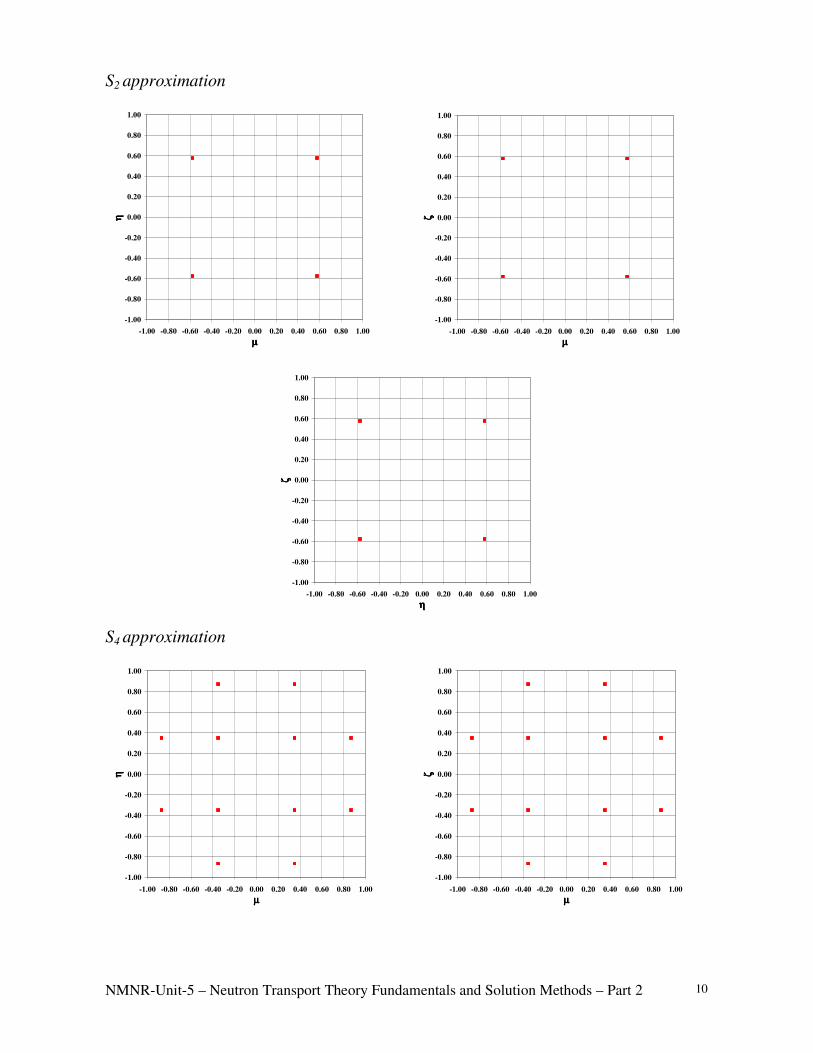
NMNR-Unit-5 – Neutron Transport Theory Fundamentals and Solution Methods – Part 2 10
S2 approximation
-1.00
-0.80
-0.60
-0.40
-0.20
0.00
0.20
0.40
0.60
0.80
1.00
-1.00 -0.80 -0.60 -0.40 -0.20 0.00 0.20 0.40 0.60 0.80 1.00
µµµµ
ηη ηη
-1.00
-0.80
-0.60
-0.40
-0.20
0.00
0.20
0.40
0.60
0.80
1.00
-1.00 -0.80 -0.60 -0.40 -0.20 0.00 0.20 0.40 0.60 0.80 1.00
µµµµ
ζζ ζζ
-1.00
-0.80
-0.60
-0.40
-0.20
0.00
0.20
0.40
0.60
0.80
1.00
-1.00 -0.80 -0.60 -0.40 -0.20 0.00 0.20 0.40 0.60 0.80 1.00
ηηηη
ζζ ζζ
S4 approximation
-1.00
-0.80
-0.60
-0.40
-0.20
0.00
0.20
0.40
0.60
0.80
1.00
-1.00 -0.80 -0.60 -0.40 -0.20 0.00 0.20 0.40 0.60 0.80 1.00
µµµµ
ηη ηη
-1.00
-0.80
-0.60
-0.40
-0.20
0.00
0.20
0.40
0.60
0.80
1.00
-1.00 -0.80 -0.60 -0.40 -0.20 0.00 0.20 0.40 0.60 0.80 1.00
µµµµ
ζζ ζζ

NMNR-Unit-5 – Neutron Transport Theory Fundamentals and Solution Methods – Part 2 11
-1.00
-0.80
-0.60
-0.40
-0.20
0.00
0.20
0.40
0.60
0.80
1.00
-1.00 -0.80 -0.60 -0.40 -0.20 0.00 0.20 0.40 0.60 0.80 1.00
ηηηη
ζζ ζζ
S6 approximation
-1.00
-0.80
-0.60
-0.40
-0.20
0.00
0.20
0.40
0.60
0.80
1.00
-1.00 -0.80 -0.60 -0.40 -0.20 0.00 0.20 0.40 0.60 0.80 1.00
µµµµ
ηη ηη
-1.00
-0.80
-0.60
-0.40
-0.20
0.00
0.20
0.40
0.60
0.80
1.00
-1.00 -0.80 -0.60 -0.40 -0.20 0.00 0.20 0.40 0.60 0.80 1.00
µµµµ
ζζ ζζ
-1.00
-0.80
-0.60
-0.40
-0.20
0.00
0.20
0.40
0.60
0.80
1.00
-1.00 -0.80 -0.60 -0.40 -0.20 0.00 0.20 0.40 0.60 0.80 1.00
ηηηη
ζζ ζζ

NMNR-Unit-5 – Neutron Transport Theory Fundamentals and Solution Methods – Part 2 12
S8 approximation
-1.00
-0.80
-0.60
-0.40
-0.20
0.00
0.20
0.40
0.60
0.80
1.00
-1.00 -0.80 -0.60 -0.40 -0.20 0.00 0.20 0.40 0.60 0.80 1.00
µµµµ
ηη ηη
-1.00
-0.80
-0.60
-0.40
-0.20
0.00
0.20
0.40
0.60
0.80
1.00
-1.00 -0.80 -0.60 -0.40 -0.20 0.00 0.20 0.40 0.60 0.80 1.00
µµµµ
ζζ ζζ
-1.00
-0.80
-0.60
-0.40
-0.20
0.00
0.20
0.40
0.60
0.80
1.00
-1.00 -0.80 -0.60 -0.40 -0.20 0.00 0.20 0.40 0.60 0.80 1.00
ηηηη
ζζ ζζ
• It can be noted that:
Increasing the order of the approximation, the unity radius sphere is gradually
populated by directions;
the directions are the same for ±90° rotations with respect to any frame axis.

NMNR-Unit-5 – Neutron Transport Theory Fundamentals and Solution Methods – Part 2 13
Results:
Cubic Source Problem
Plane z = Lz / 2
Plane z =0
Grid: 40x40x40 with S2 Approximation
The explanation of the behaviour observed on the lateral surfaces becomes evident
considering that the adimissible directions are in a too small number to provide a
sufficiently detailed representation of the scalar flux.
For instance, in the position illustrated in the following figure the 8 directions
do not intersect the source, resulting in a minimum of the scalar flux.
This occurs with perfect symmetry for any lateral surface.

NMNR-Unit-5 – Neutron Transport Theory Fundamentals and Solution Methods – Part 2 14
Cubic Source Problem
Grid: 40x40x40 with S4 Approximation
Plane z = Lz / 2
Plane z =0
Cubic Source Problem
Grid: 40x40x40 with S6 Approximation
Plane z = Lz / 2
Plane z =0

NMNR-Unit-5 – Neutron Transport Theory Fundamentals and Solution Methods – Part 2 15
Cubic Source Problem
Grid: 40x40x40 with S8 Approximation
Plane z = Lz / 2
Plane z =0
The “ray effect” is particularly clear in the case of the S2 approximation, that
provides a totally unrealistic trend of the scalar flux on the plane z = 0, to be
considered in view of the only eight admissible directaion (one per each octant).
By increasing the number of directions, the problem is mitigated, though
oscillatory trends are anyway observed, to be put in relation with ray effects.
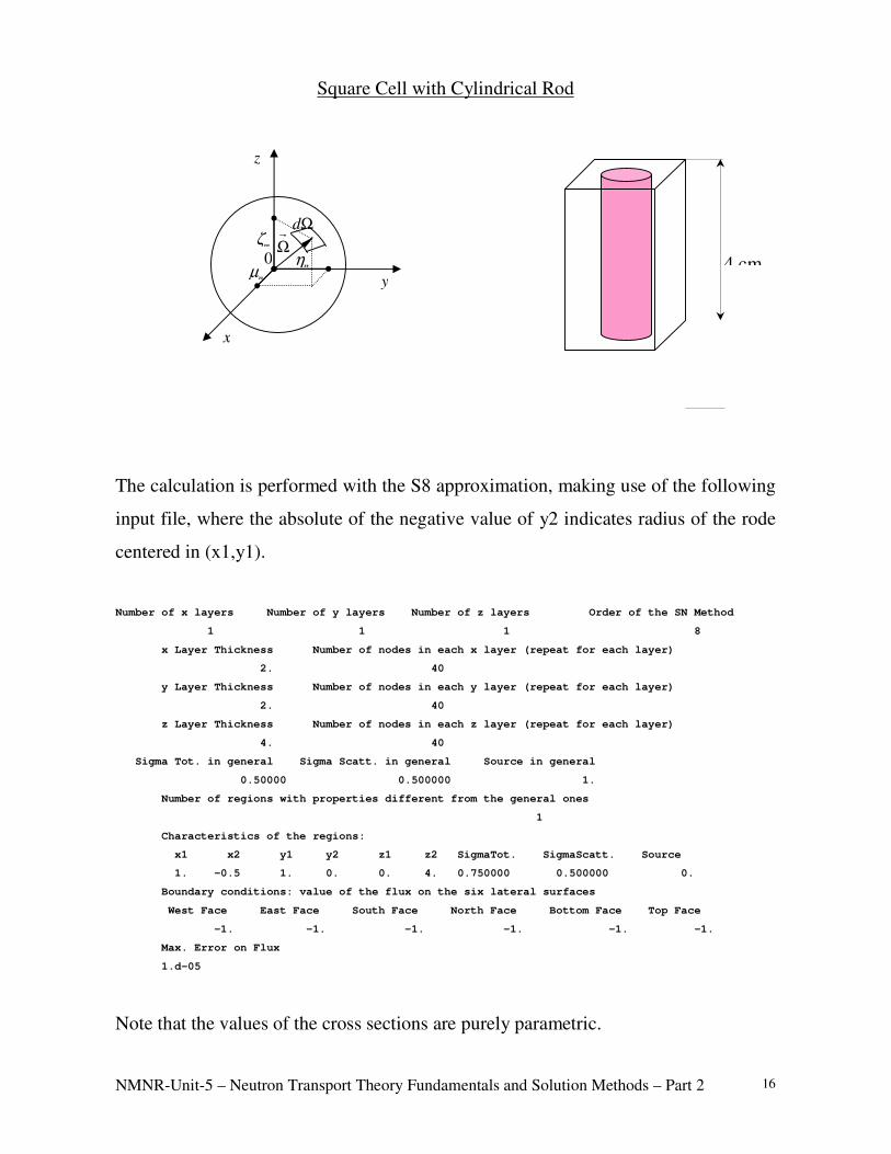
NMNR-Unit-5 – Neutron Transport Theory Fundamentals and Solution Methods – Part 2 16
Square Cell with Cylindrical Rod
The calculation is performed with the S8 approximation, making use of the following
input file, where the absolute of the negative value of y2 indicates radius of the rode
centered in (x1,y1).
Number of x layers Number of y layers Number of z layers Order of the SN Method
1 1 1 8
x Layer Thickness Number of nodes in each x layer (repeat for each layer)
2. 40
y Layer Thickness Number of nodes in each y layer (repeat for each layer)
2. 40
z Layer Thickness Number of nodes in each z layer (repeat for each layer)
4. 40
Sigma Tot. in general Sigma Scatt. in general Source in general
0.50000 0.500000 1.
Number of regions with properties different from the general ones
1
Characteristics of the regions:
x1 x2 y1 y2 z1 z2 SigmaTot. SigmaScatt. Source
1. -0.5 1. 0. 0. 4. 0.750000 0.500000 0.
Boundary conditions: value of the flux on the six lateral surfaces
West Face East Face South Face North Face Bottom Face Top Face
-1. -1. -1. -1. -1. -1.
Max. Error on Flux
1.d-05
Note that the values of the cross sections are purely parametric.
Ωm
dΩ ζm
µm
ηm0
y
z
x
4 cm

NMNR-Unit-5 – Neutron Transport Theory Fundamentals and Solution Methods – Part 2 17
The results show a classical spatial trend of the thermal flux (the source is located in
the moderator). A considerable depression of the flux is noted in the rod in the plane
z = Lz/2. Flux oscillations due to the "ray effects" are again observed.
It is also interesting to note that that along an axial plane the flus is absolutely
independent from the z coordinate, testifying for the effectiveness of the choice of
reflective boundary conditions on the top and bottom planes in transforming the 3D
problem into a 2D one.

NMNR-Unit-5 – Neutron Transport Theory Fundamentals and Solution Methods – Part 2 18
Plane z = 2 cm
Plane y = 0

NMNR-Unit-5 – Neutron Transport Theory Fundamentals and Solution Methods – Part 2 19

NMNR-Unit-5 – Neutron Transport Theory Fundamentals and Solution Methods – Part 2 20
Benchmark Problem Iron-Water
(v. H. Khalil, Nucl. Sci. Eng., 90, pp.263-280, 1985)
The problem is simulated in 3D version with reflective conditions on the faces
orthogonal to the z axis. The input file is the following
Number of x layers Number of y layers Number of z layers Order of the SN Method
1 1 1 8
x Layer Thickness Number of nodes in each x layer (repeat for each layer)
30. 30
y Layer Thickness Number of nodes in each y layer (repeat for each layer)
30. 30
z Layer Thickness Number of nodes in each z layer (repeat for each layer)
10. 10
Sigma Tot. in general Sigma Scatt. in general Source in general
3.33 3.31 0.
Number of regions with properties different from the general ones
3
Characteristics of the regions:

NMNR-Unit-5 – Neutron Transport Theory Fundamentals and Solution Methods – Part 2 21
x1 x2 y1 y2 z1 z2 SigmaTot. SigmaScatt. Source
0. 12. 0. 12. 0. 10. 3.33 3.31 1.
15. 21. 0. 21. 0. 10. 1.33 1.105 0.
0. 21. 15. 21. 0. 10. 1.33 1.105 0.
Boundary conditions: value of the flux on the six lateral surfaces
West Face East Face South Face North Face Bottom Face Top Face
-40. 0. -40. 0. -40. -40.
Max. Error on Flux
1.d-05
It can be noted that the average value of the flux in region 1 is 4.09e01, in in
agreement with tabulated data.
4. Proposed activities
• Analyse the computer program trying to indentify the following phases of the
calculation:
assignement of directions and of the related weights;
solution of the transport equation in agreement with the sign of direction
cosines;
updating the emission density.

NMNR-Unit-5 – Neutron Transport Theory Fundamentals and Solution Methods – Part 2 22
c---------------------------------------------------------------------c
c c
c Program for the solution of the integrodifferential equation c
c for transport in 3D geometry c
c c
c This programme has been set up for teaching purposes c
c and was not subjected to a sifficiently thorough validation c
c to assure the quantitative correctness of the results c
c c
c W. Ambrosini, DIMNP, Dicember 2000 c
c c
c---------------------------------------------------------------------c
program tras3d
implicit double precision (a-h,o-z)
c
include 'tras3dc.for'
c
open (unit=5,file='schermo.dat')
open (unit=6,file='tras3d.out')
open (unit=7,file='tras3d.ord')
open (unit=8,file='trasxy.txt')
open (unit=9,file='trasxz.txt')
open (unit=10,file='trasyz.txt')
open (unit=11,file='trasxy1.txt')
open (unit=12,file='trasxz1.txt')
open (unit=13,file='trasyz1.txt')
open (unit=14,file='trasxy2.txt')
open (unit=15,file='trasxz2.txt')
open (unit=16,file='trasyz2.txt')
c
c Pi is calculaetd
c
pi = 4.d00 * datan (1.d00)
c
c Reading the number of layers along the thtee axes and of the order of the method
c
read (5,*)
read (5,*) nlax,nlay,nlaz,nordin
c
c Reading of the thickness of the layer and assignment of the node coordinates (x)
c
read (5,*)
c
x(1) = 0.d00
i = 1
c
do ilax = 1,nlax
read (5,*) deltx,nlx
dx = deltx / dfloat (nlx)
c
do ix = 1,nlx
i = i + 1
x(i) = x(i-1) + dx
xm(i-1) = x(i-1) + 0.5d00 * dx
enddo
c
enddo
c
nx = i - 1
c
c Reading of the thickness of the layer and assignment of the node coordinates (y)
c
read (5,*)
c
y(1) = 0.d00
j = 1
c
do ilay = 1,nlay
read (5,*) delty,nly
dy = delty / dfloat (nly)
c
do iy = 1,nly
j = j + 1
y(j) = y(j-1) + dy
ym(j-1) = y(j-1) + 0.5d00 * dy
enddo
c
enddo
c
ny = j - 1
c
c Reading of the thickness of the layer and assignment of the node coordinates (z)
c
read (5,*)
c
z(1) = 0.d00
k = 1
c
do ilaz = 1,nlaz
read (5,*) deltz,nlz
dz = deltz / dfloat (nlz)

NMNR-Unit-5 – Neutron Transport Theory Fundamentals and Solution Methods – Part 2 23
c
do iz = 1,nlz
k = k + 1
z(k) = z(k-1) + dz
zm(k-1) = z(k-1) + 0.5d00 * dz
enddo
c
enddo
c
nz = k - 1
c
c Reading of cross sections and of the source for general nodes
c
read (5,*)
read (5,*) sigmat,sigmas,sourt
c
do i = 1,nx
do j = 1,ny
do k = 1,nz
sigt(i,j,k) = sigmat
sigs(i,j,k) = sigmas
sour(i,j,k) = sourt
enddo
enddo
enddo
c
c Reading of the number and of the position of the regions having
c properties different from the general ones
c
read (5,*)
read (5,*) nreg
c
read (5,*)
read (5,*)
c
do ir = 1,nreg
read (5,*) x1,x2,y1,y2,z1,z2,sigmat,sigmas,sval
c
if(x2.gt.0.d00) then
do i = 1,nx
do j = 1,ny
do k = 1,nz
if( (xm(i).ge.x1).and.(xm(i).le.x2)
& .and.(ym(j).ge.y1).and.(ym(j).le.y2)
& .and.(zm(k).ge.z1).and.(zm(k).le.z2) ) then
sour(i,j,k) = sval
sigt(i,j,k) = sigmat
sigs(i,j,k) = sigmas
endif
enddo
enddo
enddo
c
else
radius = dabs ( x2 )
c
do i = 1,nx
distx = xm(i) - x1
c
do j = 1,ny
disty = ym(j) - y1
rad = dsqrt ( distx * distx + disty * disty )
c
do k = 1,nz
if( (rad.le.radius)
& .and.(zm(k).ge.z1).and.(zm(k).le.z2) ) then
sour(i,j,k) = sval
sigt(i,j,k) = sigmat
sigs(i,j,k) = sigmas
endif
enddo
enddo
enddo
c
endif
c
enddo
c
c Reading of the inward fluxes at the six lateral surfaces
c
read (5,*)
read (5,*)
read (5,*) phiawf,phiaef,phiasf,phianf,phiabf,phiatf
c
c Definition of the maximum erro between two subsequent iterations
c
read (5,*)
read (5,*) epsphi
c
c Assignmenet of the discrete ordinates
c

NMNR-Unit-5 – Neutron Transport Theory Fundamentals and Solution Methods – Part 2 24
call diradm
c
c Assignement of the initial value of the source and of the fluxes at previous iteration
c
do i = 1,nx
do j = 1,ny
do k = 1,nz
q(i,j,k) = sour(i,j,k)
c
oldphi(i,j,k) = 0.d00
c
enddo
enddo
enddo
c
do im = 1,nm
c
do j = 1,ny
do k = 1,nz
phiaem(j,k,im) = dabs (phiaef)
phiawm(j,k,im) = dabs (phiawf)
enddo
enddo
c
do i = 1,nx
do k = 1,nz
phiasm(i,k,im) = dabs (phiasf)
phianm(i,k,im) = dabs (phianf)
enddo
enddo
c
do i = 1,nx
do j = 1,ny
phiabm(i,j,im) = dabs (phiabf)
phiatm(i,j,im) = dabs (phiatf)
enddo
enddo
c
enddo
c
c Loop for iteration on te scattering source
c
do iscat = 1,10000000
c
call trasp
c
call sscat
c
c Cechk on convergence on flux
c
dphimx = 0.d00
c
imax = 1
jmax = 1
kmax = 1
c
do i = 1,nx
do j = 1,ny
do k = 1,nz
c
absdif = dabs ( phi(i,j,k) - oldphi(i,j,k) )
c
if(dphimx.lt.absdif) then
dphimx = absdif
imax = i
jmax = j
kmax = k
endif
c
enddo
enddo
enddo
c
write(*,100) iscat,dphimx
write(*,*) imax,jmax,kmax
write(*,*) phi(imax,jmax,kmax),oldphi(imax,jmax,kmax)
write(6,100) iscat,dphimx
c
c Criterion for stopping the iterations
c
if(dphimx.lt.epsphi) goto 10
c
c Assigning the flux at the old iterations
c
do i = 1,nx
do j = 1,ny
do k = 1,nz
c
oldphi(i,j,k) = phi(i,j,k)
c
enddo

NMNR-Unit-5 – Neutron Transport Theory Fundamentals and Solution Methods – Part 2 25
enddo
enddo
c
enddo
c
10 continue
c
nxh = nx / 2
nyh = ny / 2
nzh = nz / 2
c
c Mapa for the planes z = zmax / 2 and z = 0
c
do i = 1,nx
do j = 1,ny
c
write(8,200) xm(i),ym(j),phi(i,j,nzh)
write(11,200) xm(i),ym(j),phi(i,j,1)
write(14,200) xm(i),ym(j),phi(i,j,nz)
c
enddo
enddo
c
c Maps for the plane y = ymax / 2 and y = 0
c
do i = 1,nx
do k = 1,nz
c
write(9,200) xm(i),zm(k),phi(i,nyh,k)
write(12,200) xm(i),zm(k),phi(i,1,k)
write(15,200) xm(i),zm(k),phi(i,ny,k)
c
enddo
enddo
c
c Maps for the plane x = xmax / 2 and x = 0
c
do j = 1,ny
do k = 1,nz
c
write(10,200) ym(j),zm(k),phi(nxh,j,k)
write(13,200) ym(j),zm(k),phi(1,j,k)
write(16,200) ym(j),zm(k),phi(nx,j,k)
c
enddo
enddo
c
stop
100 format(/,1x,' Iterazione sulla Sorgente di Scattering N. ',i6,
& ' Errphi = ',e14.7,/)
200 format(3(1x,e14.7))
end
c----------------------------------------------------------------------c
c c
c Subroutine generating admissible directins in an octant c
c c
c----------------------------------------------------------------------c
subroutine diradm
implicit double precision (a-h,o-z)
c
include 'tras3dc.for'
c
c
c Assignement of the discrete ordinetes and of their weights
c
nm = nordin * ( nordin + 2 )
noct = nm / 8
c
c Parameters for the quadrature LQ2
c
if(nordin.eq.2) then
c
rsqr3 = 1.d00 / dsqrt(3.d00)
c
ami(1) = rsqr3
eta(1) = rsqr3
zeta(1) = rsqr3
c
w(1) = 1.d00
c
call rotoct (1)
c
c Parameters for the quadrature LQ4
c
elseif(nordin.eq.4) then
c
ami1 = 0.3500212d00
ami2 = dsqrt ( 1.d00 - 2.d00 * ami1 * ami1 )
c
weight = 1.d00 / 3.d00
c
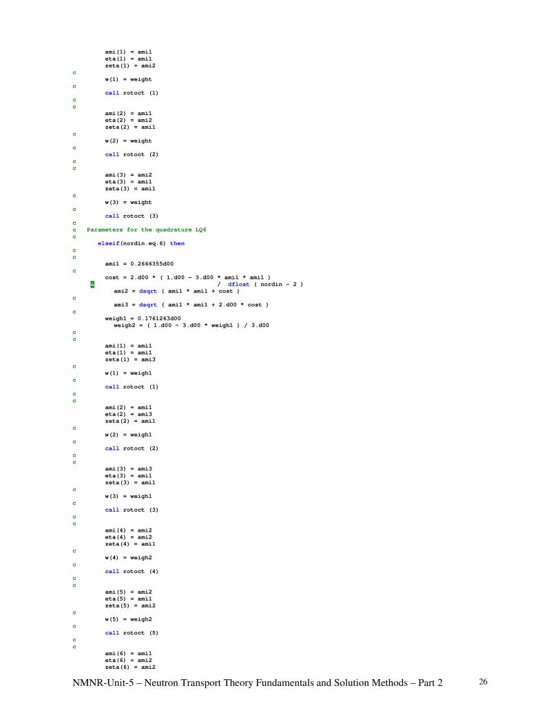
NMNR-Unit-5 – Neutron Transport Theory Fundamentals and Solution Methods – Part 2 26
ami(1) = ami1
eta(1) = ami1
zeta(1) = ami2
c
w(1) = weight
c
call rotoct (1)
c
c
ami(2) = ami1
eta(2) = ami2
zeta(2) = ami1
c
w(2) = weight
c
call rotoct (2)
c
c
ami(3) = ami2
eta(3) = ami1
zeta(3) = ami1
c
w(3) = weight
c
call rotoct (3)
c
c Parameters for the quadrature LQ6
c
elseif(nordin.eq.6) then
c
c
ami1 = 0.2666355d00
c
cost = 2.d00 * ( 1.d00 - 3.d00 * ami1 * ami1 )
& / dfloat ( nordin - 2 )
ami2 = dsqrt ( ami1 * ami1 + cost )
c
ami3 = dsqrt ( ami1 * ami1 + 2.d00 * cost )
c
weigh1 = 0.1761263d00
weigh2 = ( 1.d00 - 3.d00 * weigh1 ) / 3.d00
c
c
ami(1) = ami1
eta(1) = ami1
zeta(1) = ami3
c
w(1) = weigh1
c
call rotoct (1)
c
c
ami(2) = ami1
eta(2) = ami3
zeta(2) = ami1
c
w(2) = weigh1
c
call rotoct (2)
c
c
ami(3) = ami3
eta(3) = ami1
zeta(3) = ami1
c
w(3) = weigh1
c
call rotoct (3)
c
c
ami(4) = ami2
eta(4) = ami2
zeta(4) = ami1
c
w(4) = weigh2
c
call rotoct (4)
c
c
ami(5) = ami2
eta(5) = ami1
zeta(5) = ami2
c
w(5) = weigh2
c
call rotoct (5)
c
c
ami(6) = ami1
eta(6) = ami2
zeta(6) = ami2

NMNR-Unit-5 – Neutron Transport Theory Fundamentals and Solution Methods – Part 2 27
c
w(6) = weigh2
c
call rotoct (6)
c
c Parameters for the quadrature LQ8
c
elseif(nordin.eq.8) then
c
c
ami1 = 0.2182179d00
c
cost = 2.d00 * ( 1.d00 - 3.d00 * ami1 * ami1 )
& / dfloat ( nordin - 2 )
ami2 = dsqrt ( ami1 * ami1 + cost )
c
ami3 = dsqrt ( ami1 * ami1 + 2.d00 * cost )
c
ami4 = dsqrt ( ami1 * ami1 + 3.d00 * cost )
c
weigh1 = 0.1209877d00
weigh2 = 0.0907407d00
weigh3 = ( 1.d00 - 3.d00 * weigh1 - 6.d00 * weigh2 )
c
c
ami(1) = ami1
eta(1) = ami1
zeta(1) = ami4
c
w(1) = weigh1
c
call rotoct (1)
c
c
ami(2) = ami1
eta(2) = ami4
zeta(2) = ami1
c
w(2) = weigh1
c
call rotoct (2)
c
c
ami(3) = ami4
eta(3) = ami1
zeta(3) = ami1
c
w(3) = weigh1
c
call rotoct (3)
c
c
ami(4) = ami1
eta(4) = ami2
zeta(4) = ami3
c
w(4) = weigh2
c
call rotoct (4)
c
c
ami(5) = ami2
eta(5) = ami1
zeta(5) = ami3
c
w(5) = weigh2
c
call rotoct (5)
c
c
ami(6) = ami1
eta(6) = ami3
zeta(6) = ami2
c
w(6) = weigh2
c
call rotoct (6)
c
c
ami(7) = ami2
eta(7) = ami3
zeta(7) = ami1
c
w(7) = weigh2
c
call rotoct (7)
c
c
ami(8) = ami3
eta(8) = ami1
zeta(8) = ami2

NMNR-Unit-5 – Neutron Transport Theory Fundamentals and Solution Methods – Part 2 28
c
w(8) = weigh2
c
call rotoct (8)
c
c
ami(9) = ami3
eta(9) = ami2
zeta(9) = ami1
c
w(9) = weigh2
c
call rotoct (9)
c
c
ami(10) = ami2
eta(10) = ami2
zeta(10) = ami2
c
w(10) = weigh3
c
call rotoct (10)
c
endif
c
do im = 1,nm
c
c Assignement of the corresponding diretions by rotation around the coordinate axes
c
do imr = 1,nm
if ( (ami(imr).eq.-ami(im)).and.(eta(imr).eq.eta(im))
& .and.(zeta(imr).eq.zeta(im)) ) irx(im) = imr
if ( (ami(imr).eq.ami(im)).and.(eta(imr).eq.-eta(im))
& .and.(zeta(imr).eq.zeta(im)) ) iry(im) = imr
if ( (ami(imr).eq.ami(im)).and.(eta(imr).eq.eta(im))
& .and.(zeta(imr).eq.-zeta(im)) ) irz(im) = imr
enddo
c
c Check on the normalisation of direction cosines
c
check = ami(im)*ami(im) + eta(im)*eta(im) + zeta(im)*zeta(im)
c
write(7,100) im,ami(im),eta(im),zeta(im),w(im),check
c
enddo
c
return
100 format(1x,i5,5(1x,e14.7))
end
c----------------------------------------------------------------------c
c c
c Subroutine to generate direction in the octants with c
c negative direction cosine c
c c
c----------------------------------------------------------------------c
subroutine rotoct (i)
implicit double precision (a-h,o-z)
c
include 'tras3dc.for'
c
im = i + noct
c
c ami < 0 , eta > 0 , zeta > 0
c
w(im) = w(i)
c
ami(im) = - eta(i)
eta(im) = ami(i)
zeta(im) = zeta(i)
c
c ami < 0 , eta < 0 , zeta > 0
c
im = i + noct * 2
c
w(im) = w(i)
c
ami(im) = - ami(i)
eta(im) = - eta(i)
zeta(im) = zeta(i)
c
c ami > 0 , eta < 0 , zeta > 0
c
im = i + noct * 3
c
w(im) = w(i)
c
ami(im) = eta(i)
eta(im) = - ami(i)
zeta(im) = zeta(i)
c

NMNR-Unit-5 – Neutron Transport Theory Fundamentals and Solution Methods – Part 2 29
c ami > 0 , eta > 0 , zeta < 0
c
im = i + noct * 4
c
w(im) = w(i)
c
ami(im) = ami(i)
eta(im) = eta(i)
zeta(im) = - zeta(i)
c
c ami < 0 , eta > 0 , zeta < 0
c
im = i + noct * 5
c
w(im) = w(i)
c
ami(im) = - eta(i)
eta(im) = ami(i)
zeta(im) = - zeta(i)
c
c ami < 0 , eta < 0 , zeta < 0
c
im = i + noct * 6
c
w(im) = w(i)
c
ami(im) = - ami(i)
eta(im) = - eta(i)
zeta(im) = - zeta(i)
c
c ami > 0 , eta < 0 , zeta < 0
c
im = i + noct * 7
c
w(im) = w(i)
c
ami(im) = eta(i)
eta(im) = - ami(i)
zeta(im) = - zeta(i)
c
return
end
c----------------------------------------------------------------------c
c c
c Subroutine for solving 3D transport equations c
c c
c----------------------------------------------------------------------c
subroutine trasp
implicit double precision (a-h,o-z)
c
include 'tras3dc.for'
c
c Zeroing the scalar flux
c
do i = 1,nx
do j = 1,ny
do k = 1,nz
c
phi(i,j,k) = 0.d00
c
enddo
enddo
enddo
c
c Loop on the directions
c
do im = 1,nm
c
write(*,100) im
write(6,100) im
100 format(1x,' Processamento della direzione ',i6)
c
c Discussion of the sign of direction cosines and
c boundary conditions: assignef flux or reflection
c
c
c BC along the x axis
c
if(ami(im).gt.0.d00) then
i1 = 1
i2 = nx
ist = 1
c
do j = 1,ny
do k = 1,nz
if(phiawf.ge.0.d00) then
phiax(1,j,k) = phiawf
else
phiax(1,j,k) = phiawm(j,k,irx(im))
endif
enddo

NMNR-Unit-5 – Neutron Transport Theory Fundamentals and Solution Methods – Part 2 30
enddo
c
else
i1 = nx
i2 = 1
ist = - 1
c
do j = 1,ny
do k = 1,nz
if(phiaef.ge.0.d00) then
phiax(nx+1,j,k) = phiaef
else
phiax(nx+1,j,k) = phiaem(j,k,irx(im))
endif
enddo
enddo
c
endif
c
c BC along the y axis
c
if(eta(im).gt.0.d00) then
j1 = 1
j2 = ny
jst = 1
c
do i = 1,nx
do k = 1,nz
if(phiasf.ge.0.d00) then
phiay(i,1,k) = phiasf
else
phiay(i,1,k) = phiasm(i,k,iry(im))
endif
enddo
enddo
c
else
j1 = ny
j2 = 1
jst = - 1
c
do i = 1,nx
do k = 1,nz
if(phianf.ge.0.d00) then
phiay(i,ny+1,k) = phianf
else
phiay(i,ny+1,k) = phianm(i,k,iry(im))
endif
enddo
enddo
c
endif
c
c BC along the z axis
c
if(zeta(im).gt.0.d00) then
k1 = 1
k2 = nz
kst = 1
c
do i = 1,nx
do j = 1,ny
if(phiabf.ge.0.d00) then
phiaz(i,j,1) = phiabf
else
phiaz(i,j,1) = phiabm(i,j,irz(im))
endif
enddo
enddo
c
else
k1 = nz
k2 = 1
kst = - 1
c
do i = 1,nx
do j = 1,ny
if(phiatf.ge.0.d00) then
phiaz(i,j,nz+1) = phiatf
else
phiaz(i,j,nz+1) = phiatm(i,j,irz(im))
endif
enddo
enddo
c
endif
c
c Solution of neuutron balance equations
c sweeping the three spatial axes accordin to the sign of direction cosines
c

NMNR-Unit-5 – Neutron Transport Theory Fundamentals and Solution Methods – Part 2 31
do i = i1,i2,ist
dx = x(i+1) - x(i)
auxx = 2.d00 * dabs(ami(im)) / dx
c
do j = j1,j2,jst
dy = y(j+1) - y(j)
auxy = 2.d00 * dabs(eta(im)) / dy
c
do k = k1,k2,kst
dz = z(k+1) - z(k)
auxz = 2.d00 * dabs(zeta(im)) / dz
c
c Construction of some useful quantities
c
if(ist.eq.1) then
addx = auxx * phiax(i,j,k)
else
addx = auxx * phiax(i+1,j,k)
endif
c
if(jst.eq.1) then
addy = auxy * phiay(i,j,k)
else
addy = auxy * phiay(i,j+1,k)
endif
c
if(kst.eq.1) then
addz = auxz * phiaz(i,j,k)
else
addz = auxz * phiaz(i,j,k+1)
endif
c
c Evaluation of tye central flus by the neutron balanve
c
ifixx = 0
ifixy = 0
ifixz = 0
c
20 denom = auxx + auxy + auxz + sigt(i,j,k)
c
phiac(i,j,k) = ( addx + addy + addz + q(i,j,k) ) / denom
c
c Application of the diamond rule and, in case of negative interface flux,
c use of the "step" fix-up rule, then recalculating the central flux
c
if(ist.eq.1) then
c
if(ifixx.eq.0) then
phiax(i+1,j,k) = 2.d00 * phiac(i,j,k) - phiax(i,j,k)
else
phiax(i+1,j,k) = phiac(i,j,k)
endif
c
if(phiax(i+1,j,k).lt.0.d00) then
auxx = dabs(ami(im)) / dx
addx = auxx * phiax(i,j,k)
ifixx = ifixx + 1
c write(*,111) im,i,j,k
c write(6,111) im,i,j,k
111 format(1x,' Fix-up lungo x: direzione ',i5,' nodo ',3i6)
goto 20
endif
c
else
c
if(ifixx.eq.0) then
phiax(i,j,k) = 2.d00 * phiac(i,j,k) - phiax(i+1,j,k)
else
phiax(i,j,k) = phiac(i,j,k)
endif
c
if(phiax(i,j,k).lt.0.d00) then
auxx = dabs(ami(im)) / dx
addx = auxx * phiax(i+1,j,k)
ifixx = ifixx + 1
c write(*,111) im,i,j,k
c write(6,111) im,i,j,k
goto 20
endif
c
endif
c
if(jst.eq.1) then
c
if(ifixy.eq.0) then
phiay(i,j+1,k) = 2.d00 * phiac(i,j,k) - phiay(i,j,k)
else
phiay(i,j+1,k) = phiac(i,j,k)
endif
c
if(phiay(i,j+1,k).lt.0.d00) then

NMNR-Unit-5 – Neutron Transport Theory Fundamentals and Solution Methods – Part 2 32
auxy = dabs(eta(im)) / dy
addy = auxy * phiay(i,j,k)
ifixy = ifixy + 1
c write(*,112) im,i,j,k
c write(6,112) im,i,j,k
112 format(1x,' Fix-up lungo y: direzione ',i5,' nodo ',3i6)
goto 20
endif
c
else
c
if(ifixy.eq.0) then
phiay(i,j,k) = 2.d00 * phiac(i,j,k) - phiay(i,j+1,k)
else
phiay(i,j,k) = phiac(i,j,k)
endif
c
if(phiay(i,j,k).lt.0.d00) then
auxy = dabs(eta(im)) / dy
addy = auxy * phiay(i,j+1,k)
ifixy = ifixy + 1
c write(*,112) im,i,j,k
c write(6,112) im,i,j,k
goto 20
endif
c
endif
c
if(kst.eq.1) then
c
if(ifixz.eq.0) then
phiaz(i,j,k+1) = 2.d00 * phiac(i,j,k) - phiaz(i,j,k)
else
phiaz(i,j,k+1) = phiac(i,j,k)
endif
c
if(phiaz(i,j,k+1).lt.0.d00) then
auxz = dabs(zeta(im)) / dz
addz = auxz * phiaz(i,j,k)
ifixz = ifixz + 1
c write(*,113) im,i,j,k
c write(6,113) im,i,j,k
113 format(1x,' Fix-up lungo z: direzione ',i5,' nodo ',3i6)
goto 20
endif
else
c
if(ifixz.eq.0) then
phiaz(i,j,k) = 2.d00 * phiac(i,j,k) - phiaz(i,j,k+1)
else
phiaz(i,j,k) = phiac(i,j,k)
endif
c
if(phiaz(i,j,k).lt.0.d00) then
auxz = dabs(zeta(im)) / dz
addz = auxz * phiaz(i,j,k+1)
ifixz = ifixz + 1
c write(*,113) im,i,j,k
c write(6,113) im,i,j,k
goto 20
endif
c
endif
c
c Assignment of the contribution of the direction ot the scalar flux
c
phi(i,j,k) = phi(i,j,k) + 0.125d00 * phiac(i,j,k) * w(im)
c
c Assignement of the angular flux on thelateral surface
c to allow imposing pure reflection boundary conditions
c
if(i.eq.1) then
phiawm(j,k,im) = phiax(i,j,k)
elseif(i.eq.nx) then
phiaem(j,k,im) = phiax(nx+1,j,k)
endif
c
if(j.eq.1) then
phiasm(i,k,im) = phiay(i,j,k)
elseif(j.eq.ny) then
phianm(i,k,im) = phiay(i,ny+1,k)
endif
c
if(k.eq.1) then
phiabm(i,j,im) = phiaz(i,j,k)
elseif(k.eq.nz) then
phiatm(i,j,im) = phiaz(i,j,nz+1)
endif
c
enddo
c

NMNR-Unit-5 – Neutron Transport Theory Fundamentals and Solution Methods – Part 2 33
enddo
c
enddo
c
enddo
c
return
end
c----------------------------------------------------------------------c
c c
c Subroutine for undating the emission density c
c from the new scattering source c
c c
c----------------------------------------------------------------------c
subroutine sscat
implicit double precision (a-h,o-z)
c
include 'tras3dc.for'
c
c Assignement of density emission
c
do i = 1,nx
do j = 1,ny
do k = 1,nz
q(i,j,k) = sour(i,j,k) + sigs(i,j,k) * phi(i,j,k)
c
enddo
enddo
enddo
c
return
end

NMNR-Unit-5 – Neutron Transport Theory Fundamentals and Solution Methods – Part 2 34
Suggested personal work: new calculations cases to be analysed:
a) Benchmark Problem IAEA EIR-2 (v. H. Khalil, Nucl. Sci. Eng., 90, pp.263-280, 1985)
b) Prism with imposed inner flux
c) Different sources in a prisamtic domain
d) Parametric analyses of the already analysed cases, discussing the results
e) Comparison between the results that can be obtained by different
approximations for the angular discretisation