Lecture Notes for PHY 405Classical Mechanics

From Thorton & Marion’s Classical Mechanics

Prepared byDr. Joseph M. Hahn

Saint Mary’s UniversityDepartment of Astronomy & Physics

September 14, 2005

Chapter 3: Oscillations

SHO—simple harmonic oscillator

Start with mass m attached to a spring.

If m is displaced a distance x from equilibrium,

the spring pulls back with a force F = −kx, known as Hooke’s Law

(Robert Hooke, 1676), where k > 0 is the spring constant.

Solve this problem with Newton II, F = mr. The EOM for mass m is

or F = −kx = mx for this 1D problem

so x + ω20x = 0

where ω20 ≡ k/m

this EOM has solution x(t) = A sin(ω0t − δ)

where A = amplitude of the motion

ω0 = spring’s angular frequency (radians/time)

δ = phase constant

1

Energy of a SHO

the KE is T =1

2mx2 =

1

2mA2ω2

0 cos2(ω0t − δ)

use F = −∇U, ie F = −∂U

∂x, to get the system’s PE:

U(x) = −∫ x

0

Fdx =1

2kx2 =

1

2kA2 sin2(ω0t − δ)

so E = T + U =1

2kA2 =

1

2mA2ω2

0

or E =constant, as expected for a conservative force.

Period of a SHO

period τ = time for the motion to repeat

τ =2π

ω0= 2π

√

m

k

frequency ν0 =1

τ=

1

2π

√

k

m=

ω0

2π

Don’t confuse the angular frequency ω0 with the frequency ν0 = ω0/2π.

2

The plane pendulum

Mass m hangs at the end of a massless rod of length `.

Use Newton II, F = mr, to solve for the pendulum’s motion.

Fig. 3-13.

The pendulum is confined to a plane, so this is seemingly a 2D problem.

What is this problem’s natural coordinate system?

Choose a coordinate system that confines the motion to 1D,

ie, use polar coordinates r and θ

What is the mass’s radial acceleration? its tangential acceleration?

force perpendicular to rod Fθ = −mg sin θ

m is an arclength `θ from equilibrium position,

so its velocity = `θ and acceleration = `θ

so NII is − mg sin θ = m`θ

or θ + ω20 sin θ = 0 where ω2

0 ≡ g

`

This nonlinear EOM is discussed in greater detail in Chap. 4.

3

However we can solve this EOM when the motion is small, ie, |θ| � 1:

use small θ approx: sin θ ' θ − 1

3!θ3 +

1

5!θ5 · · · (D.28)

⇒ sin θ ' θ to lowest order in small θ

θ + ω20θ ' 0 ⇐ EOM for SHO

What is the solution to this EOM?

θ(t) ' A sin(ω0t − δ)

Initial conditions

The constants A & δ are determined by your initial conditions.

First note that θ = Aω0 cos(ω0t − δ).

Suppose your initial conditions are

θ(t = 0) = θ0 pendulum’s initial displacement˙θ(t = 0) = θ0 initial angular velocity

We need to write the express the unknown A, δ in terms of the known θ0, θ0:

then − A sin δ = θ0

and A cos δ = θ0/ω0

ratio the above: tan δ = −θ0ω0

θ0

is the phase

sum the squares: A2 = θ20 + (θ0/ω0)

2 to get the amplitude

4

Phase diagrams

Note that a particle’s trajectory, x(t), is completely specified as a function

of time once its initial conditions, x(0) and x(0) are specified.

The point P (x(t), x(t)) at some time t can be regarded as a

spot in phase space at time t.

A system with n degrees of freedom has a 2n–dimensional phase space.

As t varies over time,

P (x, x) describes the particle’s trajectory through this phase space.

To graphically illustrates the particle’s time–history, plot x(t) versus x(t).

Plotting x vs x for various initial conditions thus reveals the particle’s range

of possible motions—this is a phase diagram.

Fig. 3-5.

5

The SHO has a rather simple phase diagram:

x(t) = A sin(ω0t − δ)

x(t) = Aω0 cos(ω0t − δ)

so(x

A

)2

+

(

x

Aω0

)2

= 1,

which is the equation for an ellipse where

A = ellipse’s semimajor axis,

Aω0 = ellipse’s semiminor axis.

The phase diagram for more complicated systems, like the NL pendulum,

can be much more interesting...

Can trajectories in phase space cross?

Keep in mind that solutions to NII are unique.

6

Phase Diagram for a Nonlinear (NL) Pendulum

Fig. 3-13.

This discussion comes from Section 4.4.

Recall that the exact EOM for mass m is θ + ω20 sin θ = 0 where ω2

0 = g/`.

We say this EOM is NL due to the term sin θ = θ − θ3/6 + · · · (D.28)

First, examine the system’s PE, U(θ):

Recall that

U(θ) = −∫ θ

θref=?

F · dr

where position vector r = `θr

so differential path length dr = `dθθ

and F = Frr + Fθθ = mg cos θr − mg sin θθ

so F · dr = −mg` sin θdθ

and U(θ) = mg`

∫ θ

θref=0

sin θ′dθ′ = − mg` cos θ′|θ0

= mg`(1 − cos θ) = m`2ω20(1 − cos θ)

Note that U is periodic in θ.

7

Find the equilibrium sites θeq, which is easily done by inspecting U(θ).

More formally, θeq satisfies

∂U

∂θ

∣

∣

∣

∣

θeq

= m`2ω20 sin θeq = 0

⇒ θeq = 0,±π

Which equilibria are stable? unstable? Again, inspect U(θ).

Alternatively, check sign of k:

k =∂2U

∂θ2

∣

∣

∣

∣

θeq

= m`2ω20 cos θeq

for θeq = 0, k = m`2ω20 > 0 ⇒ stable

for θeq = ±π, k = −m`2ω20 < 0 ⇒ unstable

8

Now calculate the system’s KE, T = 12mv2.

If the end of the pendulum is moving with an angular velocity θ,

what is the pendulum’s linear velocity?

Thus T = 12m`2θ2.

The system’s total energy is

E = T + U =1

2m`2θ2 + m`2ω2

0(1 − cos θ)

=1

2m`2ω2

0

(

θ

ω0

)2

+ 2(1 − cos θ)

Is E conserved? Why?

Can we use this expression to draw a phase diagram, θ(θ)? How?

Note that(

θ

ω0

)2

+ 2(1 − cos θ) =2E

m`2ω20

≡ E ′2

where E ′2 = a (constant) dimensionless energy

9

First, consider small–amplitude motion, ie, when |θ| � 1:

cos θ ' 1 − 1

2θ2 + · · · Eqn. D.29 of text

so

(

θ

E ′ω0

)2

+

(

θ

E ′

)2

= 1

which again is the same eqn’ for an ellipse as obtained previous for the SHO:

Where is the stable equilibrium site for this system?

What would happen to these trajectories if a small amount of friction were

added to the system?

Friction causes particles to settle towards the stable equilibria;

such sites in phase space are known as attractors.

10

Now lets consider the more general case where the amplitude of the motion

|θ| is no longer small:(

θ

ω0

)2

+ 2(1 − cos θ) = E ′2

Keep in mind that the first term represents the system’s KE, the second is PE.

In particular, lets consider the case of very energetic motion,

ie, E ′ � 1 so θ/ω0 � 1 (ie, the system’s energy is nearly all KE),

while the PE term is O(1), and is negligible.

⇒ θ ' ±E ′ω0 ' constant:

Which way should the arrows point?

11

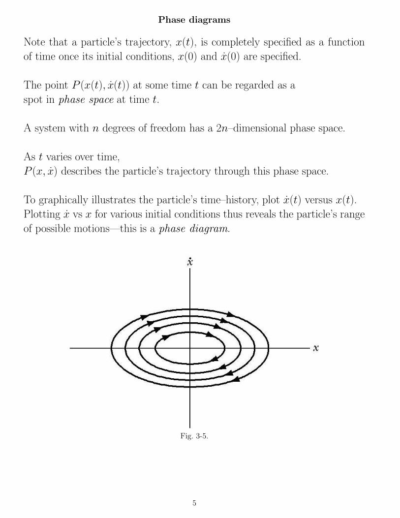
Now consider the motion of a pendulum with just enough energy

to swing up to θ = π:

What is this system’s energy, E0?

Note that in this case, θ = 0 when θ = π,

so E ′2 = 4 =2E0

m`2ω20

⇒ E0 = 2m`2ω20 = U(θ = π) as expected.

Add this trajectory to the phase diagram:

Fig. 4–11

Note that this phase diagram is periodic in θ;

The zone between −π < θ < π is referred to a unit cell; identical unit cells

also lie left & right of the central unit cell.

12

What is special about the trajectory that has energy E0?

This curve is known as the separatrix,

since it divides the phase space into two types of motion:

1. oscillatory motion: where E < E0 and |θ| < θmax, ie, the pendulum

oscillates. Here, θmax is the solution to E = U(θmax) = m`2ω20(1− cos θmax)

1. circulating motion: where E > E0 and θ is unrestricted,

ie, the pendulum rotates.

Note that the separatrix passes through the unstable equilibrium points.

Note also that in our examination of the NL pendulum, we have *not* solved

the system’s EOM. Rather, all we have done is invoked energy conservation,

and then analyzed E(θ, θ) graphically.

This graphical analysis of a physics problem can be quite handy; even tho

we have not solve the EOM analytically, we have obtained an understanding

of the range of possible motions that a NL pendulum might exhibit, by

simply sketching its phase diagram.

Problem Set #2

due ?

1. Draw a phase diagram for the system described in problem 2–43.

Locate stable and unstable equilibria in your sketch, and label the separatrix,

if present.

13

Damped SHO

Now consider mass m attached to a spring, but add friction to the problem.

Many frictional forces are proportional to velocity,

so we will adopt Ffriction = −br where constant b > 0.

What is Newton II for this problem?

F = −kx − bx = mx

so x + 2βx + ω20x = 0

where β ≡ b

2m= damping parameter, has units of frequency

and ω0 =

√

k

m= angular frequency, aka the natural oscillation frequency

Solution for when β 6= ω0:

x(t) = e−βt(A1eγt + A2e

−γt)

where A1,A2 are constant amplitudes

and γ ≡√

β2 − ω20 which can be a real or imaginary frequency

Note that the coefficients A1 and A2 can also be complex.

Nonetheless, this expression should always result in x(t) being real

since it is a physical quantity.

Additional problem for Problem Set #2:

2.A. Substitute x(t) into the EOM and verify that it is a solution.

14

Underdamped motion

Occurs when β < ω0, eg, light damping.

In this case, γ is complex:

γ = iω1

where ω21 ≡ ω2

0 − β2

so x(t) = e−βt(A1eiω1t + A2e

−iω1t)

Note that

eia = cos a + i sin a, Eqn. (D.44)

so x = e−βt [A1(cos ω1t + sin ω1t) + iA2(cos ω1t − sin ω1t)]

= e−βt [(A1 + A2) cos ω1t + i(A1 − A2) sin ω1t]

Since x(t) is real, this implies that:

A1 + A2 is real and that A1 − A2 is imaginary.

However we can always replace the 2 unknowns A1 and A2

with two other unknowns A and δ that are a little more handy:

A1 + A2 → A cos δ

i(A1 − A2) → A sin δ

so x(t) = Ae−βt(cos ω1t cos δ + sin ω1t sin δ)

Simplify further using the trig identity D.12 of Appendix D:

cos(a ± b) = cos a cos b ∓ sin a sin b

so x(t) = Ae−βt cos(ω1t − δ)

where δ = phase coefficient

⇒underdamped motion=SHO × exponential damping of the amplitude over

a e–fold damping timescale τdamp = β−1 = 2m/b.

15

Phase diagram for an underdamped SHO:

Fig. 3-10b.

The phase diagram for an underdamped SHO simply spirals towards the

equilibrium point.

Note that ω1 = is the oscillator’s natural oscillation frequency,

while T = 2π/ω1 = oscillation ‘period’

Where in this phase diagram is this particle at time t = T, 2T, 3T , etc?

Also plot x(t) for this underdamped oscillator.

16

Overdamped motion

Recall that the EOM is

x + 2βx + ω20x = 0

which has solution x(t) = e−βt(A1eγt + A2e

γt) where γ =√

β2 − ω20

Overdamped motion occurs when β > ω0, ie, the damping is heavy:

γ =√

β2 − ω20 is real

so x(t) = A1e−(β−γ)t + A2e

−(β+γ)t

where constants A1 & A2 are determined by initial conditions

overdamped systems ⇒ exponential return to equilibrium

Overdamped systems do not oscillate.

17

Critical damping

Occurs when β = ω0.

Solution x(t) = (A + Bt)e−βt.

Additional problem for Assignment #2:

2.B. show that this is a solution of the EOM.

Critical damping returns the particles to its equilibrium with the fewest

overshoots.

Examples of critically damped systems: the pneumatic tube on a screen door,

auto shock absorbers.

Fig. 3-6.

18

Problem Set #2

due Tuesday October 4

at start of class

Problems 1, 2A, 2B, & text problems 3–7, 3–11, 3–40, 3–42, 3–45.

Example 3.3

A pendulum of mass m and length ` moves through oil that resists the motion

with force Fres = −2m√

g/`(`θ). The bob is initially released from position

θ = θ0. Find the motion, θ(t), θ(t), and sketch the system’s phase diagram.

Fig. 3-13.

What coordinate system should we use?

Asses the forces:

gravitational Fgrav = mg cos θr − mg sin θθ

frictional Fres = −2m√

g/`(`θ)θ

Note that the radial forces balance: T = mg cos θ

19

the θ force: Fθ = −mg sin θ − 2m√

g/`(`θ) = maθ

What is the acceleration aθ in the θ direction? `θ,

so the EOM is θ + 2

√

g

`θ +

g

`sin θ = 0

or θ + 2βθ + ω20 sin θ = 0

where β =

√

g

`and ω2

0 =g

`For small displacements sin θ ' θ

so θ + 2βθ + ω20θ = 0

Is the bob’s motion underdamped? Overdamped?

Since β = ω0, the motion is critically damped.

What is the solution for the bob’s motion?

Recall that θ(t) = (A + Bt)e−βt where constants A, B

are determined by initial conditions: θ(0) = θ0 and θ(0) = 0

⇒ A = θ0.

Since θ = [B − β(A + Bt)]e−βt = 0 when t = 0 ⇒ B = βA so

θ(t) = θ0(1 + βt)e−βt

θ(t) = −θ0β2te−βt

20

Note that θ → 0 when t � Tdamping,

where Tdamping = 1/β is the damping timescale.

Also note that the angular velocity θ initially grows

(in a negative sense) as θ ' −θ0β2t when t � Tdamping,

but that θ → 0 when t � Tdamping.

Ultimately, all trajectories dive for the origin in the phase diagram:

Fig. 3-14.

Are there any attractors in this phase diagram?

21

Sinusoidal Driving Forces

Again, lets consider mass m attached to spring k that rests on a place with

friction coefficient b.

But now add a sinusoidal driving force F0 cos(ωt) due to a piston that is also

pushing on m:

force F (t) = −kx − bx + F0 cos(ωt) = mx

so x + 2βx + ω20x = A cos(ωt)

where A = F0/m = the driving acceleration, and ω = driving frequency.

The general solution is

x(t) = xc(t) + xp(t)

where xc(t) = complimentary solution, ie, the solution for when A = 0

and xp(t) = particular solution, ie, the solution for when A 6= 0

Note that we have already obtained the complimentary solution:

xc(t) = e−βt(A1eγt + A2e

−γt)

where γ =√

β2 − ω20

xc is called the transient part of the solution since it decays away as ∼ e−βt.

The constants A1 and A2 will depend on initial conditions x(0) and x(0).

However the system eventually ‘loses memory’ of initial conditions

(eg, A1, A2) later when t � Tdamping = 1/β.

22

Now get the particular solution xp:

Insert x = xc + xp into the EOM.

Obviously, only the xp terms survive:

xp + 2βxp + ω20xp = A cos(ωt)

Since the driving force ∝ cos(ωt),

we likely need a similar term in the particular solution. Try

xp(t) = D cos(ωt − δ) where amplitude D and phase-shift δ are constants

It will be convenient to expand xp using trig identity D.12:

cos(a ± b) = cos a cos b ∓ sin a sin b

so xp = D cos(ωt − δ) = D(cosωt cos δ + sin ωt sin δ)

and xp = ωD(− sin ωt cos δ + cos ωt sin δ)

and xp = ω2D(− cos ωt cos δ − sin ωt sin δ)

Insert these into equation of motion and collect sin ωt and cos ωt terms:

cos ωt{−ω2D cos δ + 2βωD sin δ + ω20D cos δ − A]+

sin ωt[−ω2D sin δ − 2βωD cos δ + ω20D sin δ} = 0

or cos ωt{−A + D[(ω20 − ω2) cos δ + 2βω sin δ]}+

sin ωtD{(ω20 − ω2) sin δ − 2βω cos δ} = 0

Note that the LHS must be zero for any time t.

What does this say about the coefficients in the {}?

23

the sin ωt coefficient yields

(ω20 − ω2) sin δ = 2βω cos δ

sosin δ

cos δ= tan δ =

2βω

ω20 − ω2

≡ Y

X

thus sin δ =Y√

X2 + Y 2=

2βω√

(ω20 − ω2)2 + (2βω)2

and cos δ =X√

X2 + Y 2=

ω20 − ω2

√

(ω20 − ω2)2 + (2βω)2

Note that the driving force has a phase ωt,

while the system’s response has the phase ωt − δ,

so δ is the phase difference that exists between the driving force and the

response of the system; it is a consequence of friction, β.

Now get the amplitude D from the coefficient of the cos ωt term:

D[(ω20 − ω2) cos δ + 2βω sin δ] = A

so D =A

(ω20 − ω2) cos δ + 2βω sin δ

= A/[(ω20 − ω2)2 + (2βω)2]/

√

(ω20 − ω2)2 + (2βω)2

=A

√

(ω20 − ω2)2 + (2βω)2

D is often referred to as the system’s forced amplitude.

It is usually convenient to think of D(ω) and δ(ω)

as functions of the driving frequency ω.

24

The complete solution for the motion of the damped/driven oscillator is

x(t) = xc + xp = xc + D(ω) cos[ωt − δ(ω)]

where the complimentary (ie, transient) solution xc decays away as e−βt.

The steady–state part, xp, is usually the more interesting part of the solution.

Note that all of the information about the system’s initial conditions,

x(0) and ˙x(0), are contained in the transient part xc,

so the system eventually loses memory of its initial state as xc → 0.

Resonances

When building a driven oscillator, the driving frequency ω is usually tunable.

Often you are interested in determining the driving frequency ω that maxi-

mizes the system’s response D(ω).

This occurs are the resonant frequency ω = ωR:

write D(ω) =A

√

f(ω)

where f(ω) = (ω20 − ω2)2 + (2βω)2

The resonance frequency ωR is obtained by setting df/dω|ωR= 0, ie

2(ω20 − ω2

R)(−2ωR) + 8β2ωR = 0

so ω20 − ω2

R = 2β2 or ωR =√

ω20 − 2β2

Note that for a lightly damped system with β � ω0,

the resonance frequency is nearly the system’s naturally oscillation frequency,

ωR ' ω0.

25

Fig. 3-16.

Recall that

D(ω) =A

√

(ω20 − ω2)2 + (2βω)2

= response to driving force

and sin δ =2βω

√

(ω20 − ω2)2 + (2βω)2

and cos δ =ω2

0 − ω2

√

(ω20 − ω2)2 + (2βω)2

Another characteristic of a resonance is that the system’s response is

in–phase when ω � ωR. For a lightly damped system (β � ω0)

sin δ ' 2βω/ω20 � 1 ⇒ δ ' 0.

But when ω � ωR, cos δ ' −1 ⇒ δ ' π

Plots of D(ω) and δ(ω) can all be parameterized by a

dimensionless ‘quality factor’ Q:

Q =ωR

2β

26

Q is a dimensionless measure of the friction in your oscillator.

It is also an indicator of the ‘width’ of the resonance,

Example: an audio speaker is a driven/damped oscillator, typically has

Q ∼ 100.

Electronic circuits, like a stereo receiver tuned to a radio station, has

Q ∼ 104, while lasers can have Q ∼ 1010.

The Fig. shows that a high–Q system (ie. one with small friction β)

has as large response (ie. large D(ω)) at the resonant frequency ω = ωR.

Simple example

Springs k1 and k2 = 2k1 are attached to mass m which slides with friction

coefficient b or β = b/2m =√

k1/100m. What is this system’s Q?

the EOM is F = −k1x − k2x − bx = mx

so x + ω20x + 2βx = 0

where ω20 = (k1 + k2)/m = 3k1/m = natural osc’ freq’2

the resonant frequency is ωR =√

ω20 − 2β2

=

√

3k1

m− 2k1

100m=

√

298k1

100m

and Q =ωR

2β=

√

298k1/100m

2√

k1/100m=

√298

2' 8.6

Not an especially high–quality oscillator...

27

Superposition of Discrete Driving Forces

Thus far we have considered a damped SHO driven by a single sinusoidal

force F (t) = mA cos(ωt):

the EOM is x + ω20x + 2βx = A cos(ωt)

and its solution is x(t) = xc(t) + xp(t)

where xc = complimentary (or transient) part, is damped by friction,

and xp = D cos(ωt − δ) = particular solution (eg, the forced response).

What if there two distinct driving forces operating with different frequencies:

F (t)/m = A1 cos(ω1t − φ1) + A2 cos(ω2t − φ2)?

How will the system’s forced solution xp change?

(Note that the driving force has acquired a phase φ;

to account for this, simply replace ωt → ωt − φ in the solution.)

We anticipate that xp = D1 cos(ω1t − φ1 − δ1) + D2 cos(ω2t − φ2 − δ2)

⇒ for each driving acceleration An operating at frequency ωn,

the system responds with a displacement xn(t) = Dn cos(ωnt − φn − δn).

And if there are N distinct driving forces

F (t) =N∑

n=1

Fn(t) = mN∑

n=1

An cos(ωnt − φn)

we anticipate the solution is x(t) = xc(t) + xp(t) = xc +∑

xn(t).

28

To verify this solution, insert x = xc + xp into the EOM:

xp + ω20xp + 2βxp = F/m.

Recall that the contribution from the transient part, xc, sum to zero, so

N∑

n=1

[

xn + ω20xn + 2βxn − An cos(ωnt − φn)

]

= 0

Note that the xn and its derivatives are sinusoids in ωnt, which means that

they are drawn from a complete set of orthogonal functions.

What does this say about the quantity in the []?

⇒ xn + ω20xn + 2βxn = An cos(ωnt − φn)

and we already know the solution to this eqn:

xn(t) = Dn cos(ωnt − φn − δn)

where Dn(ωn) =An

√

(ω20 − ω2

n)2 + (2βωn)2= amplitude of nth response

and tan δn =2βωn

ω20 − ω2

n

= nth phase shift

The total solution is x(t) = xc(t)+∑

xn(t) where xc is the transient response,

determined by initial conditions.

29

Continuous Spectrum of Driving Forces

We just solve for the motion of a damped SHO when it is driven by a

combination of N discrete forces F (t) =∑

Fn

that operate at N discrete frequencies ωn.

However this solution might not appear to be very useful, since it might not

be widely applicable.

We would much rather have the solution to the more general problem where

F (t) = any arbitrary driving force that is periodic over time T = 2π/ω:

How can we use the preceding results to solve this more general problem?

We would like to replace F (t) with∑

Fn(t),

since we know the solution to the EOM in this case.

To do this, Fourier expand the driving force F (t), that is, assume that

F (t)

m=

1

2a0 +

∞∑

n=1

[an cos(nωt) + bn sin(nωt)]

which can also be written as =∞∑

n=0

An cos(nωt − φn) via trig identity

Note we have replaced the nth driving frequency ωn → nω, where ω = 2π/T .

30

The solution to the EOM has the usual form x(t) = xc + xp where

xp =∞∑

n=0

xn(t)

where xn(t) = Dn cos(nωt − φn − δn)

where Dn and δn are (since ωn → nω):

Dn(ω) =An

√

(ω20 − n2ω2)2 + (2βnω)2

and tan δn =2βnω

ω20 − n2ω2

Applying these results to the problem of a damped SHO

that is driven by an arbitrary force F (t) that is periodic in time T = 2π/ω

requires doing the following calculations:

1. Fourier expand F (t) to get the an, bn coefficients

2. relating the an, bn to the An, φn

3. Forming the solution x(t) = xc +∑

xn

4. Satisfying initial conditions x(0) and x(0),

which yields the A1, A2 appearing in xc = e−βt(A1eγt + A2e

−γt)

31

Example: a damped SHO driven by a sawtooth function

This calculation come from example 3.6, and will illustrate the above 4 steps.

A SHO having natural oscillation frequency ω0 and a damping frequency β

is driven by a sawtooth function:

Fig. 3-19.

F (t)

m=

At

τover time −τ/2 < t < τ/2,

and repeating over other times.

What is the driving frequency ω?

32

Step 1: Fourier expand F (t)

Assume that F (t) can be written as

F (t)

m=

1

2a0 +

∞∑

n=1

[an cos(nωt) + bn sin(nωt)]

To get the an coefficient, multiply by cos(n′ωt) where n′ = unspecified int’,

and integrate over one forcing cycle τ = 2π/ω:

1

m

∫ τ/2

−τ/2

F (t) cos(n′ωt)dt =

∞∑

n=1

an

∫ τ/2

−τ/2

cos(nωt) cos(n′ωt)dt

use trig identity, from D.12 cos α cos β =1

2cos(α + β) +

1

2cos(α − β)

so cos(nωt) cos(n′ωt) =1

2cos[(n + n′)ωt] +

1

2cos[(n − n′)ωt]

and RHS =∞∑

n=1

1

2an

∫ τ/2

−τ/2

{cos[(n + n′)ωt] + cos[(n − n′)ωt]}dt

Consider only single nth term in this sum.

When n 6= n′, what do these integrals evaluate to?

What about the n = n′ term?

⇒ RHS =1

2an′

∫ τ/2

−τ/2

dt

=τ

2an′ =

π

ωan′

⇒ an =ω

π

∫ τ/2

−τ/2

F (t)

mcos(nωt)dt

How do you solve for the bn?

bn =ω

π

∫ τ/2

−τ/2

F (t)

msin(nωt)dt

These are the general formulae for the an, bn.

33

sawtooth example

F (t)

m=

At

τ

so an =Aω

πτ

∫ τ/2

−τ/2

t cos(nωt)dt

Note that the integrand f(t) = t cos(nωt) is odd, ie f(−t) = −f(t).

What does this say about the an?

An even function has f(−t) = f(t).

so bn =Aω

πτ

∫ τ/2

−τ/2

t sin(nωt)dt

u–substitution: u = nωt so du = nωdt

and bn =Aω

πτ (nω)2

∫ +nωτ/2=+nπ

−nπ

u sin(u)du

=A

2π2n2(sin u − u cos u)|+nπ

−nπ

=A

2π2n2[sin(nπ) − sin(−nπ) − nπ cos(nπ) − nπ cos(−nπ)]

= −A cos(nπ)

πn= −A(−1)n

πn=

A(−1)n+1

πn

34

sawtooth example

ThusF (t)

m=

At

τ=

∞∑

n=1

bn sin(nωt)

=A

π

[

sin(ωt) − 1

2sin(2ωt) +

1

3sin(3ωt) · · ·

]

Fig. 3-20.

In practice, one keeps simply sums enough terms in the infinite series that

your representation of the force F (t) is sufficiently accurate.

35

Step 2: Get the An, φn from the an, bn

Recall that in general,

F (t)

m=

1

2a0 +

∞∑

n=1

[an cos(nωt) + bn sin(nωt)] =

∞∑

n=0

An cos(nωt − φn)

=∞∑

n=0

[An cos(nωt) cos φn + An sin(nωt) sin φn] by (D.12)

⇒ an = An cos φn and bn = An sin φn

so An =√

a2n + b2

n and tan φn = bn/an

back to sawtooth example

In this case, An = |bn| = A/πn,

while tan φn = bn/an is problematic for this example.

Instead use bn = An sin φn = |bn| sin φn

⇒ sin φn = sgn(bn) = (−1)n+1 = ±1

so φn = (−1)n+1π

2

36

Step 3: form the solution

form the solution x(t) = xc +∞∑

n=0

xn

where xc(t) = e−βt(A1eγt + A2e

−γt) = transient solution

xn(t) = Dn cos(nωt − φn − δn) = nth forced solution

where Dn(ω) =An

√

(ω20 − n2ω2)2 + (2βnω)2

and tan δn =2βnω

ω20 − n2ω2

for the sawtooth problem

An =A

πn

so Dn(ω) =A/πn

ω20 − n2ω2

What is δn for this system?

and x = xc + xp = xc + x1 + x2 + x3 · · ·

= xc +A cos(ωt − π/2)

π(ω20 − ω2)

+A cos(2ωt + π/2)

2π(ω20 − 4ω2)

+A cos(3ωt − π/2)

3π(ω20 − 9ω2)

· · ·

37

Step 4: determine initial conditions

ie, adjust the A1 and A2 in the transient solution xc = e−βt(A1eγt +A2e

−γt)

so that initial conditions can be satisfied.

sawtooth

Suppose initial conditions x(0) = 0 and x(0) = 0

note that xp(0) = 0 ⇒ xc = 0

so A1 = −A2

also xc = γA1 − γA2 = 0 at time t = 0

⇒ A1 = A2

What does this say about the sawtooth oscillator’s transient motion?

What are the resonant frequencies for the sawtooth oscillator?

What is the system’s response when driven near its nth resonance?

In this case, the system’s response is dominated by the nth resonant term:

x(t) ' xn =A cos[nωt + (−1)nπ/2]

nπ(ω20 − n2ω2)

38