Lecture Notes for Math 414: Linear Algebra II Fall 2015 ......... v= av+ bv If F = R, \real vector...

$: Lecture Notes for Math 414: Linear Algebra II Fall 2015 ......... v= av+ bv If F = R, \real vector space" If F = C, \complex vector space" From here on out V will always denote a vector$
Lecture Notes for Math 414: Linear Algebra IIFall 2015, Michigan State University

Matthew Hirn

December 11, 2015

Beginning of Lecture 1

1 Vector Spaces

What is this course about?

1. Understanding the structural properties of a wide class of spaces whichall share a similar additive and multiplicative structurestructure = “vector addition and scalar multiplication”→ vector spaces

2. The study of linear maps on finite dimensional vector spaces

We begin with vector spaces. First two examples:

1. Rn = n-tuples of real numbers x = (x1, . . . , xn), xk ∈ Rvector addition: x+y = (x1, . . . , xn)+(y1, . . . , yn) = (x1+y1, . . . , xn+yn)scalar multiplication: λ ∈ R, λx = λ(x1, . . . , xn) = (λx1, . . . , λxn)

2. Cn [on your own: review 1.A on complex numbers]

1.B Definition of Vector Space

Scalars: Field F (assume F = R or C unless otherwise stated). So the previoustwo vector spaces can be written as Fn with scalars F

Let V be a set (for now).

1

Fall 2015 Math 414: Linear Algebra II

Definition 1 (Vector addition). u, v ∈ V , assigns an element u+ v ∈ V

Definition 2 (Scalar multiplication). λ ∈ F, v ∈ V , assigns an elementλv ∈ V

Definition 3 (Vector space). A set V is a vector space over the field F ifvector addition and scalar multiplication are defined, and the following prop-erties hold (u, v, w ∈ V , a, b ∈ F):

1. Commutativity: u+ v = v + u

2. Associativity: (u+ v) + w = u+ (v + w) and (ab)v = a(bv)

3. Additive Identity: ∃ 0 ∈ V such that v + 0 = v

4. Additive Inverse: for every v there exists w such that v + w = 0

5. Multiplicative Identity: 1v = v

6. Distributive Properties: a(u+ v) = au+ av and (a+ b)v = av + bv

If F = R, “real vector space”If F = C, “complex vector space”

From here on out V will always denote a vector space

Two more examples of vector spaces:

1. F∞: x = (x1, x2, . . .) just like Fn

2. FS = the set of functions f : S → F from S to F [check on your own]

Now for some important properties...

Proposition 1. The additive identity is unique.

Proof. Let 01 and 02 be any two additive identities. Then

01 = 01 + 02 = 02 + 01 = 02

Proposition 2. The additive inverse is unique.

2


Proof. Let w1 and w2 be two additive inverses of v. Then:

w1 = w1 + 0 = w1 + (v + w2) = (v + w1) + w2 = 0 + w2 = w2

Now we can write −v as the additive inverse of v and define subtraction asv−w = v+ (−w). On the other hand, we still don’t “know” that −1v = −v!

Notation: We have 0F and 0V . In the previous two propositions we dealt with0V . Next we will handle 0F. We just write 0 for either and use the context todetermine the meaning.

Proposition 3. 0Fv = 0V for every v ∈ V

Proof.0v = (0 + 0)v = 0v + 0v =⇒ 0v = 0

Now the other way around...

Proposition 4. λ0 = 0 for every λ ∈ F

Proposition 5. (−1)v = −v for all v ∈ V

Proof.v + (−1)v = 1v + (−1)v = (1 + (−1))v = 0v = 0

Now use uniqueness of additive inverse.

End of Lecture 1

3



Warmup: Is the empty set ∅ a vector space?Answer: No since 0 /∈ ∅

1.C Subspaces

A great way to find “new” vector spaces is to identify subsets of an existingvector space which are closed under addition and multiplication.

Definition 4 (Subspace). U ⊂ V is a subspace of V if U is also a vectorspace (using the same vector addition and scalar multiplication as V ).

Proposition 6. U ⊂ V is a subspace if and only if:

1. 0 ∈ U

2. u,w ∈ U =⇒ u+ w ∈ U

3. λ ∈ F and u ∈ U =⇒ λu ∈ U

Now we can introduce more interesting examples of vector spaces, many ofwhich are subspaces of FS for some set S [you should verify these are vectorspaces]:

1. P(F) = {p : F→ F : p(z) = a0 + a1z + · · · amzm︸︷︷︸deg(p)=m

, ak ∈ F ∀ k,m ∈ N}

2. C(R;R) = real valued continuous functions

3. Cm(Rn;R) = real valued functions with continuous partial derivativesup to order m

4. R([0, 1]) = {f : [0, 1]→ R :∫ 1

0 f(x) dx <∞}.

5. Fm,n = the set of all m× n matrices with entries in F

6. S = {x : [0, 1]→ Rn : x′(t) is continuous and x′(t) = Ax(t), where A ∈Rn,n}

Another convenient way to get new vector spaces is to add subspaces together(this is like the union of two sets, but for vector spaces!).

4


Definition 5 (Sum of subsets). Suppose U1, . . . , Um ⊂ V . Then:

U1 + · · ·+ Um := {u1 + · · ·+ um : u1 ∈ U1, . . . , um ∈ Um}.

Proposition 7. Suppose U1, . . . , Um are subspaces of V . Then U1 + · · ·+Umis the smallest subspace of V containing U1, . . . , Um.

An example:

U1 = {x ∈ R3 : x1 + x2 + x3 = 0}U2 = {x ∈ R3 : x3 = 0}

U1 + U2 = {x ∈ R3 : x = y + z, y1 + y2 + y3 = 0 and z3 = 0}U1 + U2 = {x ∈ R3 : x = a(−1, 0, 1) + b(1,−1, 0) + c(1, 0, 0) + d(0, 1, 0)}

(1)

U1 + U2 = R3

Note there is redundancy in (1). We will be especially interested in situationsthat avoid this redundancy, i.e., subspace summations U1 + · · · + Um whenthe representation u1 + · · ·+ um is unique.

Definition 6 (Direct sum). Suppose that U1, . . . , Um are subspaces of V .

• U1 + · · · + Um is a direct sum if each element of U1 + · · · + Um can bewritten in only one way as u1 + · · ·+ um where uk ∈ Uk.

• If U1 + · · ·+ Um is a direct sum, then we denote it as U1 ⊕ · · · ⊕ UmExamples:

1. Let Uk be the subspace of Fn such that only the kth coordinate isnonzero:

Uk = {(0, . . . , 0︸︷︷︸k−1

, x, 0, . . . , 0) : x ∈ F}

ThenRn = U1 ⊕ · · · ⊕ Un

2. Recall the previous example with redundancy. That is not a direct sum.We can change U2 though to get a direct sum:

U1 = {x ∈ R3 : x1 + x2 + x3 = 0}U2 = {x ∈ R3 : x1 = x2 = x3}R3 = U1 ⊕ U2

5


Notice in the second example that U1∩U2 = {0}. This leads us to the followingproposition.

Proposition 8. Let U,W be subspaces of V . Then,

V = U ⊕W ⇐⇒ U ∩W = {0}

The first example makes it tempting to propose the same pairwise inter-section property for any number of subspaces, but this is not true! [try tocome up with an example, then see the book] Instead we have the followingproposition, which we can use to prove Proposition 8.

Proposition 9. Suppose U1, . . . , Um are subspaces of V . Then

U1 + · · ·+ Um is a direct sum ⇐⇒0 = u1 + · · ·+ um, uk ∈ Uk, only when uk = 0 ∀ k

Proof. The ⇒ direction is clear.For the ⇐ direction, let v ∈ U1 + · · · + Um and suppose we have two repre-sentations:

v = u1 + · · ·+ um = w1 + · · ·+ wm

Then0 = (u1 − w1) + · · ·+ (um − wm)

Since uk − wk ∈ Uk, we must have uk = wk for each k.

[try to prove Proposition 8 on your own using Proposition 9, then see thebook].

2 Finite Dimensional Vector Spaces

2.A Span and Linear Independence

We saw last time that summing subspaces gives rise to new vector spaces.Now we keep track of each of the vectors that generate these spaces.

Definition 7 (Linear combination). w is a linear combination of the vectorsv1, . . . , vm ∈ V if ∃ a1, . . . , am ∈ F such that

w = a1v1 + · · · amvm

6


Definition 8 (Span). The span of v1, . . . , vm ∈ V is

span(v1, . . . , vm) = {a1v1 + · · · amvm : ak ∈ F ∀ k}

Analogous to the sum of subspaces, we have the following result.

Proposition 10. span(v1, . . . , vm) is the smallest subspace of V containingv1, . . . , vm.

Nomenclature: If span(v1, . . . , vm) = V then we say that v1, . . . , vm spans V .

Definition 9 (Finite dimensional vector space). V is finite dimensional ifthere exists a finite number of vectors v1, . . . , vm (a list) such that span(v1, . . . , vm) =V .

Definition 10 (Infinite dimensional vector space). V is infinite dimensionalif it is not finite dimensional.

End of Lecture 2

7



Warmup: Is this a vector space?

1. {f ∈ C((0, 1);R) : f(x) = x−p for some p > 0}Answer: No (all three properties fail)

2. {f ∈ C(R;R) : f is periodic of period σ}Answer: Yes (contains zero function, closed under addition and scalarmultiplication)

Examples:

1. P(F) is infinite dimensional [see the proof in the book].

2. Pm(F) = {p ∈ P(F) : deg(p) ≤ m} is finite dimensional:

span(1, z, z2, . . . , zm) = Pm(F)

3. U = {f ∈ C(R;R) : f is periodic of period n for some n ∈ N}U is infinite dimensional

Proof. Let L = v1, . . . , vm be an arbitrary list from U , so that each vkhas period nk ∈ N. If ` = lcm(n1, . . . , nm), then any linear combinationfrom L will have period which is at most `. Therefore if p is a primenumber such that p > `, sin(2π

p x) /∈ L, but sin(2πp x) ∈ U , and thus

span(L) 6= U . Since L was arbitrary we can conclude that no finite listwill span U .

It will be very useful to record if a list of vectors v1, . . . , vm has no redundancyin its span, just as we isolated sums of subspaces with no redundancy bydefining the direct sum.

Definition 11 (Linear independence). v1, . . . , vm ∈ V are linearly independentif whenever 0 = a1v1 + · · ·+ amvm, then necessarily a1 = · · · = am = 0.

Definition 12 (Linear dependence). v1, . . . , vm ∈ V are linearly dependentif ∃ a1, . . . am with at least one ak 6= 0 and 0 = a1v1 + · · ·+ amvm.

The notions of linear independence and linear dependence are extremely im-portant!

Examples:

8


1. (1, 0, 0), (0, 1, 0) are linearly independent in F3

2. 1, z, . . . , zm are linearly independent in P(F) [Why? Use the fact thata polynomial of degree m has at most m distinct zeros]

3. Recall example from sum of subspaces:

• (−1, 0, 1), (1,−1, 0), (1, 0, 0), (0, 1, 0) are linearly dependent

• (−1, 0, 1), (1,−1, 0), (1, 1, 1) are linearly independent

The following is a very useful lemma...

Lemma 1 (Linear Dependence Lemma, LDL). If v1, . . . , vm ∈ V are linearlydependent and v1 6= 0, then ∃ k ∈ {2, . . . ,m} such that

1. vk ∈ span(v1, . . . , vk−1)

2. If the vk is removed from v1, . . . , vm then the resulting span is the sameas the original.

Proof. Let L = v1, . . . , vm. For #1, by definition of linear dependence ∃ a1, . . . , amnot all zero such that 0 = a1v1 + · · ·+amvm. Let k ∈ {2, . . . ,m} be the largestindex such that ak 6= 0. Then:

vk = −a1

akv1 − · · · −

ak−1

akvk−1 (2)

For #2, let L∗ = L \ {vk}. Since L∗ ⊂ L, span(L∗) ⊂ span(L). Let u ∈span(L). Then:

u = a1v1 + ak−1vk−1 + akvk + ak+1vk+1 + · · ·+ amvm

Substitute (2) in for vk and the sum is now in terms of L∗, i.e., u ∈ span(L∗).Thus span(L) ⊂ span(L∗).

Now for our first theorem.

Theorem 1. If V = span(v1, . . . , vn) and w1, . . . , wm are linearly independentin V , then m ≤ n.

9


Proof. We will use the two lists and make successive reductions and additionsusing Lemma 1.Note: w1, . . . , wm linearly indpendent ⇒ wk 6= 0 ∀ k [why?]

Add & reduce: Since V = span(v1, . . . , vn) and w1 ∈ V , then w1, v1, . . . , vnare linearly dependent. So Lemma 1 says at least one of the vk can be re-moved. Up to a relabeling, we may assume it is vn. So span(w1, v1, . . . , vn−1)is the same as span(v1, . . . , vn).

Now we can repeat: w2 ∈ V = span(w1, v1, . . . , vn−1) so w2, w1, v1, . . . , vn−1

are linearly dependent. Use Lemma 1 again, which says that one of them canbe removed. The question is which? If it is w1, then w1 ∈ span(w2), which isa contradiction; so it must be one of the v1, . . . , vn−1. Without loss of gener-ality (WLOG), we may assume it is vn−1 and so span(w2, w1, v1, . . . , vn−2) =span(w2, v1, . . . , vn−1) = V .

Keep repeating. At each stage one of the vk must be removed, else Lemma 1implies that wj ∈ span(w1, . . . wj−1) which is a contradiction.

The process stops when either we run out of w’s (m ≤ n) or we run outof v’s (m > n). If m > n, then span(w1, . . . , wn) = V and m > n. Thuswm /∈ span(w1, . . . , wn) = V , but this is a contradiction since wk ∈ V ∀ k.

Proposition 11. If V is finite dimensional and U is a subspace of V , thenU is finite dimensional.

End of Lecture 3

10



2.B Bases

span+ linear independence = basis

Definition 13. v1, . . . , vn ∈ V is a basis of V if span(v1, . . . , vn) = V andv1, . . . , vn are linearly independent.

Proposition 12. v1, . . . , vn ∈ V is a basis of V if and only if∀ v ∈ V, ∃! a1, . . . , an ∈ F such that

v = a1v1 + · · · anvn

The notion of a basis is extremely important because it allows us to define acoordinate system for our vector spaces!

Examples:

1. (1, 0, . . . , 0), (0, 1, 0, . . . , 0), . . . , (0, . . . , 0, 1) is the standard basis of Fn.

2. 1, z, . . . , zm is the standard basis for Pm(F)

3. Let ZN = {0, 1, . . . , N − 1} (with addition mod N) and let V = {f :ZN → C}. The standard (time side) basis for V is δ0, . . . , δN−1 where

δk(n) =

{1 n = k0 n 6= k

Indeed,

f(n) =N−1∑k=0

f(k)δk(n)

Fourier analysis tells us that another (frequency side) basis for V ise0, . . . , eN−1 where

ek(n) =1√Ne2πikn/N

and

f(n) =N−1∑k=0

akek(n)

11


with

ak = f(k) =1√N

N−1∑n=0

f(n)e−2πikn/N

The coefficients ak define the function f(k) which is the Fourier transformof f .

If v1, . . . , vn spans V , it should have enough vectors to make a basis. Indeed:

Proposition 13. If L = v1, . . . , vn spans V , then L can be reduced to a basis.

Proof. If L is linearly independent, then we are done. So assume it is not.We will selectively throw away vectors using the LDL.

Step 1: If v1 = 0 remove v1

Step 2: If v2 ∈ span(v1), remove v2

Step k: If vk ∈ span(v1, . . . , vk−1), remove vk

Stop at Step n, getting a new list L∗ = w1, . . . , wm. We still have span(L∗) =V since we only discarded vectors that were in the span of other vectors. Wealso have the property:

wk /∈ span(w1, . . . , wk−1), ∀ k > 1

Thus by the contrapositive of LDL, L∗ is linearly independent, and hence abasis.

Corollary 1. If V is finite dimensional, it has a basis.

We just removed stuff from a spanning set to get a basis. We can also addstuff to a linearly independent set to get a basis.

Proposition 14. If L = u1, . . . , um ∈ V is linearly independent, then L canbe extended to a basis.

Proof. Let w1, . . . , wn be a basis of V . Thus

L∗ = u1, . . . , um, w1, . . . , wn

spans V . Apply the procedure in the proof of Proposition 13, and note thatnone of the u’s get deleted [why?].

12


Now we show that every subspace U has a complementary subspace W thattogether direct sum to V .

Proposition 15. Suppose V is finite dimensional and that U is a subspaceof V . Then there exists another subspace W such that

V = U ⊕W

Proof. V finite dimensional⇒U finite dimensional⇒ U has a basis u1, . . . , um.By the previous proposition we can extend u1, . . . , um to a basis of V , sayL = u1, . . . , um, w1, . . . , wn. We show that W = span(w1, . . . , wn) is the an-swer.

We need to show: (1) V = U + W , and (2) U ∩ W = {0}. Since L is abasis, for any v ∈ V we have:

v = a1u1 + · · ·+ amum︸︷︷︸u∈U

+ b1w1 + · · ·+ bnwn︸︷︷︸w∈W

= u+ w ∈ U +W

Now suppose that v ∈ U ∩W . Then

v = a1u1 + · · ·+ amum = b1w1 + · · ·+ bnwn

which implies

a1u1 + · · ·+ amum − b1w1 − · · · − bnwn = 0

But L is linearly independent so a1 = · · · = am = b1 = · · · = bn = 0.

2.C Dimension

Since a basis gives a unique representation of each v ∈ V , we should be ableto say that the number of vectors in basis is the dimension of V . But to doso, we need to make sure every basis of V has the same number of vectors.Indeed:

Theorem 2. Any two bases of a finite dimensional vector space have thesame length.

Proof. Let B1 = v1, . . . , vm and B2 = w1, . . . , wn be two bases of V . Since B1

is linearly independent and B2 spans V , m ≤ n. Flipping the roles of B1 andB2, we get n ≤ m.

13


Definition 14. The dimension of V is the length of B for any basis B.

Proposition 16. If U is a subspace of V , then dimU ≤ dimV

Examples:

1. dimFn = nRemark: dimR2 = 2 and dimC = 1, even though R2 can be identi-fied with C. The scalar field F cannot be ignored when computing thedimension of V !

2. dimPm(F) = m+ 1

Let L = v1, . . . , vn. If dimV = n, then we need only check if L is linearlyindependent OR if span(L) = V to conclude that L is a basis for V .

Proposition 17. Suppose dimV = n and let L = v1, . . . , vn.

1. If L is linearly independent, then L is a basis

2. If span(L) = V , then L is a basis.

Proof. Use Proposition 14 for (1) and Proposition 13 for (2).

End of Lecture 4

14



Theorem 3. dimV <∞, U1 and U2 subspaces of V . Then

dim(U1 + U2) = dimU1 + dimU2 − dim(U1 ∩ U2)

Proof. Proof will use 3 objects:

1. B = u1, . . . , um = basis of U1 ∩ U2

2. L1 = v1, . . . , vj = extension of B so that B ∪ L1 = basis for U1

3. L2 = w1, . . . , wk = extension of B so that B ∩ L2 = basis for U2.

We will show that L = B ∪L1 ∪L2 is a basis for U1 +U2. This will completethe proof since if it is true, then

dim(U1+U2) = m+j+k = (m+j)+(m+k)−m = dimU1+dimU2−dim(U1∩U2)

Clearly L spans U1 + U2 since span(L) contains both U1 and U2.

Now we show linear independence. Suppose:∑i

aiui +∑l

blvl +∑p

cpwp = 0 (3)

Then: ∑p

cpwp = −∑i

aiui −∑l

blvl ∈ U1

But wp ∈ U2 by assumption, so∑p

cpwp ∈ U1 ∩ U2 ⇒∑p

cpwp =∑q

dquq for some dq

Now, (u1, . . . , um, w1, . . . , wk) is a basis for U2. Thus:∑p

cpwp −∑q

dquq = 0⇒ cp = 0, dq = 0, ∀ p, q

Therefore (3) reduces to ∑i

aiui +∑l

blvl = 0

Repeat the previous argument.

15


3 Linear Maps

V,W always vector spaces.

3.A The Vector Space of Linear Maps

Definition 15. Let V,W be vector spaces over the same field F. A functionT : V → W is a linear map if it has the following two properties:

1. additivity: T (u+ v) = Tu+ Tv, ∀u, v ∈ V

2. homogeneity: T (λv) = λ(Tv) ∀λ ∈ F, v ∈ V

The set of all linear maps from V to W is denoted L(V,W ).

Note: You could say T is linear if it “preserves the vector space structures ofV and W .”

Examples (read the ones in the book too!):

• Fix a point x0 ∈ R. Evaluation at x0 is a linear map:

T : C(R;R)→ RTv = v(x0)

• The anti-derivative is a linear map:

T : C(R;R)→ C1(R;R)

(Tv)(x) =

∫ x

0

v(y) dy

• Fix b ∈ F. Define the forward shift operator as:

T : F∞ → F∞

T (v1, v2, v3, . . .) = (b, v1, v2, v3, . . .)

T is a linear map if and only if b = 0 [why?].

Next we show that we can always find a linear map that takes whatevervalues we want on a basis, and furthermore, that it is completely determinedby these values.

16


Theorem 4. Let v1, . . . , vn be a basis for V and let w1, . . . , wn ∈ W . Thenthere exists a unique linear map T : V → W such that

Tvk = wk, ∀ k

Proof. Define T : V → W as

T (a1v1 + · · · anvn) = a1w1 + · · ·+ anwn

Clearly Tvk = wk for all k. It is easy to see that T is linear as well [see thebook].

For uniqueness, let S : V → W be another linear map such that Svk = wkfor all k. Then:

S(a1v1+· · · anvn) =n∑k=1

S(akvk) =n∑k=1

akSvk =n∑k=1

akwk = T (a1v1+· · ·+anvn)

The previous theorem is elementary, but highlights the fact that amongst allthe maps from V to W , linear maps are very special.

Theorem 5. L(V,W ) is a vector space with the following vector addition andscalar multiplication operations:

• vector addition: S, T ∈ L(V,W ), (S + T )(v) = Sv + Tv ∀ v ∈ V

• scalar mult.: T ∈ L(V,W ), λ ∈ F, (λT )(v) = λ(Tv) ∀ v ∈ V

Theorem 6. L(V,W ) is finite dimensional and

dimL(V,W ) = (dimV )(dimW )

Proof. Suppose dimV = n and dimW = m and let

BV = v1, . . . , vnBW = w1, . . . , wm

be bases for V and W respectively. Define the linear transform Ep,q : V → Was

Ep,q(vk) =

{0 k 6= qwp k = q

, p = 1, . . . ,m, q = 1, . . . , n

17


By Theorem 4, this uniquely defines each Ep,q. We are going to show thatthese mn transformations {Ep,q}p,q form a basis for L(V,W ).

Let T : V → W be a linear map. For each 1 ≤ k ≤ n, let a1,k, . . . , am,kbe the coordinates of Tvk in the basis BW :

Tvk =m∑p=1

ap,kwp

To prove spanning, we wish to show that:

T =m∑p=1

n∑q=1

ap,qEp,q (4)

Let S be the linear map on the right hand side of (4). Then for each k,

Svk =∑p

∑q

ap,qEp,qvk

=∑p

ap,kwp

= Tvk

So S = T , and since T was arbitrary, {Ep,q}p,q spans L(V,W ).

To prove linear independence, suppose that

S =∑p

∑q

ap,qEp,q = 0

Then Svk = 0 for each k, so∑p

ap,kwp = 0, ∀ k

But w1, . . . , wm are linearly independent, so ap,k = 0 for all p and k.

End of Lecture 5

18



Warmup: Let U,W be 5-dimensional subspaces of R9. Can U ∩W = {0}?Answer: No. First note that dim{0} = 0. Then, using Theorem 3 we have:

dimR9 = 9 ≥ dim(U1 + U2) = dimU1 + dimU2 − dim(U1 ∩ U2)

= 10− dim(U1 ∩ U2)

⇒ dim(U1 ∩ U2) ≥ 1

Proposition 18. If T : V → W is a linear map, then T (0) = 0.

Proof.T (0) = T (0 + 0) = T (0) + T (0)⇒ T (0) = 0

Usually the product of a vector from one vector space with a vector fromanother vector space is not well defined. However, for some pairs of linearmaps, it is useful to define their product.

Definition 16. If T ∈ L(U, V ) and S ∈ L(V,W ), then the product ST ∈L(U,W ) is

(ST )(u) = S(Tu), ∀u ∈ U

Note: You must make sure the range of T is in the domain of S!Another note: Multiplication of linear maps is not commutative! In otherwords, in general ST 6= TS.

3.B Null Spaces and Ranges

For a linear map T , the collection of vectors that get mapped to zero and thecollection of those that do not are very important.

Definition 17. For T ∈ L(V,W ), the null space of T , nullT , is:

nullT = {v ∈ V : Tv = 0}

See examples in the book.

Proposition 19. For T ∈ L(V,W ), nullT is a subspace of V .

19


Proof. Check if it contains zero, closed under addition, closed under scalarmultiplication:

• T (0) = 0 so 0 ∈ nullT

• u, v ∈ nullT , then T (u+ v) = Tu+ Tv = 0 + 0 = 0

• u ∈ nullT , λ ∈ F, then T (λu) = λTu = λ0 = 0

Definition 18. A function T : V → W is injective if Tu = Tv implies u = v.

Proposition 20. Let T ∈ L(V,W ). Then

T is injective⇐⇒ nullT = {0}

Proof. For the ⇒ direction, we already know that 0 ∈ nullT . Thus T (v) =0 = T (0), but since T is injective v = 0.

For the ⇐ direction, we have:

Tu = Tv ⇒ T (u− v) = 0⇒ u− v = 0⇒ u = v

Definition 19. For T : V → W , the range of T is:

rangeT = {Tv : v ∈ V }

Proposition 21. If T ∈ L(V,W ), then rangeT is a subspace of W .

Definition 20. A function T : V → W is surjective if rangeT = W .

Theorem 7 (Rank-Nullity Theorem). Suppose V is finite dimensional andT ∈ L(V,W ). Then rangeT is finite dimensional and

dimV = dim(nullT ) + dim(rangeT )

Proof. Let u1, . . . , um be a basis for nullT , and extend it to a basis u1, . . . , um, v1, . . . , vnof V . So we need to show that dim rangeT = n. To do so we prove thatTv1, . . . , T vn is a basis for rangeT .

20


Let v ∈ V and write:

v = a1u1 + · · ·+ amum + b1v1 + · · ·+ bnvn⇒ Tv = b1Tv1 + · · ·+ bnTvn

Thus span(Tv1, . . . , T vn) = rangeT

Now we show that Tv1, . . . , T vn are linearly independent. Suppose

c1Tv1 + · · ·+ cnTvn = 0

⇒ T (c1v1 + · · ·+ cnvn) = 0

⇒ c1v1 + · · ·+ cnvn ∈ nullT

⇒ c1v1 + · · ·+ cnvn = d1u1 + · · ·+ dmum

But v1, . . . , vn, u1, . . . , um are linearly independent, so cj = dk = 0 for all j, k.Thus Tv1, . . . , T vn are linearly independent.

Corollary 2. Suppose V,W are finite dimensional and let T ∈ L(V,W ).Then:

1. If dimV > dimW then T is not injective.

2. If dimV < dimW then T is not surjective.

Proof. Use the Rank-Nullity Theorem:

1. dim nullT = dimV − dim rangeT ≥ dimV − dimW > 0

2. dim rangeT = dimV − dim nullT ≤ dimV < dimW

End of Lecture 6

21


Beginning of Lecture 7Very important applications:

• Homogeneous systems of equationsm equations and n unknowns:

n∑k=1

a1,kxk = 0

... (5)n∑k=1

am,kxk = 0

where aj,k ∈ F and x = (x1, . . . , xn) ∈ Fn.Can you solve all m equations simultaneously? Clearly x = 0 is a solu-tion. Are there any others? Define T : Fn → Fm:

T (x1, . . . , xn) =

(n∑k=1

a1,kxk, . . . ,

n∑k=1

am,kxk

)(6)

Note: T (0) = 0 is equivalent to saying 0 is a solution of (5). Further-more,

Nontrivial solutions exist for (5)⇐⇒ dim nullT > 0

But by the Rank-Nullity Theorem:

dim nullT > 0⇐⇒ dimFn − dim rangeT > 0

Since dim rangeT ≤ m,

if n > m =⇒ Nontrivial solutions exist for (5)

• Inhomogeneous systems of equations: Let ck ∈ F and consider:

n∑k=1

a1,kxk = c1

... (7)n∑k=1

am,kxk = cm

22


New question, can you say for all c = (c1, . . . , cm) ∈ Fm there exists atleast one solution to (7)? Using the same T as defined in (6), we have:

A solution exists for (6)⇐⇒ ∀c ∈ Fm,∃x ∈ Fn s.t. T (x) = c

⇐⇒ rangeT = Fm

⇐⇒ dim rangeT = m

⇐⇒ dimFn − dim nullT = m

⇐⇒ dim nullT = n−m

Since dim nullT ≥ 0, if n < m then certainly there exists c ∈ Fm suchthat no solution exists for (7).

3.C Matrices

Definition 21. Let T ∈ L(V,W ) and let BV = v1, . . . , vn and BW = w1, . . . , wmbe bases of V andW respectively. The matrix of T with respect to BV and BWis the m×n matrixM(T ;BV ,BW ) (or justM(T ) when BV and BW are clear)with entries Aj,k defined by:

Tvk =m∑j=1

Aj,kwj, ∀ k = 1, . . . , n

Note: Recall the proof of the fact that dimL(V,W ) = mn. In that proof wewere implicitly using the matrix representation of T .

Another note: Recall the idea that a basis BV = v1, . . . , vn for a vector spaceV gives coordinates for V . That is, for all v ∈ V , there exists a1, . . . , an ∈ Fsuch that

v = a1v1 + · · ·+ anvn

So the n-tuple (a1, . . . , an) ∈ Fn is a coordinate representation of the vector vin the basis BV . If we change the basis, say to B′V , we change the coordinaterepresentation of v say to (a′1, . . . , a

′n), but we do not change v.

Similarly, the matrix M(T ;BV ,BW ) can be thought of as a coordinate rep-resentation of the linear map T ∈ L(V,W ) with respect to the bases BV andBW . If we change the bases, we get a new matrix representation of T , but wedo not change T ; it is still the same linear map. [we will come back to thiswith an example later]

23


Definition 22. Fm,n is the set of all m× n matrices with entries in F.

Proposition 22. Fm,m is a vector space with the standard matrix additionand scalar multiplication.

Proposition 23. dimFm,n = mn.

We will derive matrix multiplication from the desire thatM(ST ) =M(S)M(T )for all S, T for which ST makes sense. Suppose T : U → V , S : V → W ,and that BV = {vr}nr=1 is basis for V , BW = {wj}mj=1 is a basis for W , andBU = {uk}pk=1 is a basis for U . LetM(S) = A andM(T ) = C. Then for each1 ≤ k ≤ p:

(ST )uk = S

(∑r=1

nCr,kvr

)

=n∑r=1

Cr,kSvr

=n∑r=1

Cr,k

m∑j=1

Aj,rwj

=m∑j=1

(n∑r=1

Aj,rCr,k

)wj

Thus we define matrix multiplication as:

(AC)j,k =n∑r=1

Aj,rCr,k

[read the rest of 3.C on matrix multiplication on your own]

End of Lecture 7

24



3.D Invertibility and Isomorphic Vector Spaces

Definition 23. A linear map that is both injective and surjective is calledbijective.

Definition 24. A linear map T ∈ L(V,W ) is invertible if ∃S ∈ L(W,V )such that ST = IV and TS = IW . Such a map S is an inverse of T .

Proposition 24. An invertible linear map has a unique inverse.

Proof. Let S1 and S2 be two inverses of T ∈ L(V,W ). Then:

S1 = S1I = S1(TS2) = (S1T )S2 = IS2 = S2

Notation: Thus we can denote the inverse of T as T−1 ∈ L(W,V ).

Theorem 8.

T ∈ L(V,W ) is invertible⇐⇒ T is bijective

Proof. For the =⇒ direction: Need to show T is injective and surjective.Suppose:

Tv1 = Tv2 ⇒ T−1Tv1 = T−1Tv2 ⇒ v1 = v2

since T−1T = I. Thus T is injective.Now suppose w ∈ W . Then:

TT−1w = w ⇒ T (T−1w)︸︷︷︸∈V

= w

and so T is surjective.

Now for the ⇐= direction: Need to show T is invertible. To do so we de-fine a map S ∈ L(W,V ) and show that ST = I and TS = I.Define S : W → V as:

Sw := unique v ∈ V s.t. Tv = w (i.e., Sw = v ⇔ Tv = w)

25


Note S is well defined only because T is bijective! By construction we haveTS = I. To show that ST = I, let v ∈ V , then:

T (STv) = (TS)(Tv) = Tv ⇒ ST = I since T is injective

Now we need to show that S ∈ L(W,V ). For additivity let w1, w2 ∈ W :

T (Sw1 + Sw2) = TSw1 + TSw2 = w1 + w2

⇒ S(w1 + w2) = Sw1 + Sw2 by definition of S

For homogeneity use a similar argument:

T (λSw) = λT (Sw) = λw ⇒ S(λw) = λSw

We now want to formalize the notion of when two vector spaces are essentiallythe same.

Definition 25. Two parts:

• An isomorphism is an invertible linear map (i.e., a bijection)

• V,W are isomorphic if there exists T ∈ L(V,W ) such that T is anisomorphism. We write V ∼= W .

Theorem 9.V ∼= W ⇐⇒ dimV = dimW

Proof. For the =⇒ direction, we know then there is a bijection T ∈ L(V,W ).Thus nullT = {0} and rangeT = W , so by Rank-Nullity Theorem:

dimV = dim nullT + dim rangeT = 0 + dimW = dimW

For the ⇐= direction, let v1, . . . , vn be a basis for V and let w1, . . . , wn be abasis for W . Define T : V → W as:

T (c1v1 + · · ·+ cnvn) = c1w1 + · · · cnwn

It is easy to see T ∈ L(V,W ), T is injective, T is surjective. Thus T definesan isomorphism.

Corollary 3. If dimV = n, then V ∼= Fn.

26


Remark: This proves that we can think of the coordinates of any v ∈ V in abasis BV = v1, . . . , vn as a unique representation in Fn, with the vector spacestructure of V carried over to Fn. Indeed, define the matrix of v ∈ V withrespect to the basis BV as the n× 1 matrix:

M(v;BV ) :=

c1...cn

where

v = c1v1 + · · ·+ cnvn

The linear map M(·,BV ) : V → Fn (note Fn,1 ∼= Fn trivially) is an isomor-phism.

Corollary 4. If dimV = n and dimW = m, then L(V,W ) ∼= Fm,n.

Proof. This follows easily since we already proved that dimL(V,W ) = (dimV )(dimW ).

Proposition 25. Let BV = v1, . . . , vn be a basis of V and let BW = w1, . . . , wmbe a basis of W . Then M(·;BV ,BW ) : L(V,W )→ Fm,n is an isomorphism.

Proposition 26. Let T ∈ L(V,W ), let v ∈ V , and let BV and BW be basesof V and W respectively. Then:

M(Tv;BW ) =M(T ;BV ,BW )M(v;BV )

[See the book for the proofs of the previous two propositions.]

Example: Let D ∈ L(P3(R),P2(R)) be the differentiation operator, definedby Dp = p′. Let’s compute the matrix M(D) of D with respect to thestandard bases B3 = 1, x, x2, x3 of P3(R) and B2 = 1, x, x2 of P2(R). SinceDxn = (xn)′ = nxn−1 we have:

M(D;B3,B2) =

0 1 0 00 0 2 00 0 0 3

End of Lecture 8

27



Example: Let D ∈ L(P3(R),P2(R)) be the differentiation operator, definedby Dp = p′. Let’s compute the matrix M(D) of D with respect to thestandard bases B3 = 1, x, x2, x3 of P3(R) and B2 = 1, x, x2 of P2(R). SinceDxn = (xn)′ = nxn−1 we have:

M(D;B3,B2) =

0 1 0 00 0 2 00 0 0 3

Now lets consider a different basis for P3(R), for example B′3 = 1 + x, x +x2, x2 + x3, x3. Compute:

D(1 + x) = 1

D(x+ x2) = 1 + 2x

D(x2 + x3) = 2x+ 3x2

D(x3) = 3x2

Thus:

M(D;B′3,B2) =

1 1 0 00 2 2 00 0 3 3

Now consider the specific polynomial p ∈ P3(R),

p(x) = 2 + x+ 3x2 + 5x3 =⇒ p′(x) = 1 + 6x+ 15x2

The coordinates of p in B3 and B′3, as well as p′ in B2, are:

M(p;B3) =

2135

M(p;B′3) =

2−141

M(p′;B2) =

1615

Computing Dp in terms of matrix multiplication with respect to B3 and B2

28


we should get back M(p′;B2); indeed:

M(Dp;B2) =M(D;B3,B2)M(p;B3)

=

0 1 0 00 0 2 00 0 0 3

2135

=

1615

=M(p′;B2)

We should also be able to compute Dp in terms of matrix multiplication butwith respect to B′3 and B2 and still get back M(p′;B2); indeed:

M(Dp;B2) =M(D;B′3,B2)M(p;B′3)

=

1 1 0 00 2 2 00 0 3 3

2−141

=

1615

=M(p′;B2)

Remark: As we said earlier, the choice of bases determines the matrix rep-resentation M(T ;BV ,BW ) of the linear map T ∈ L(V,W ). Later on we willprove important results about the choice of the bases the give the “nicest”possible matrix representation of T .

Definition 26. A linear map T ∈ L(V, V ) =: L(V ) is an operator.

Remark: For the matrix of an operator T ∈ L(V ), we assume that we takethe same basis BV for both the domain V and the range V , and thus writeit as M(T ;BV ) := M(T ;BV ,BV ). Furthermore, M(T ;BV ) ∈ Fn,n, wheredimV = n, and so we see that M(T ;BV ) is a square matrix.

Theorem 10. Suppose V is finite dimensional and T ∈ L(V ). Then thefollowing are equivalent:

29


1. T is bijective (i.e., invertible)

2. T is surjective

3. T is injective

Remark: Not true if V is infinite dimensional!

Proof. We prove this by proving that 1⇒ 2⇒ 3⇒ 1.Clearly 1⇒ 2 so that part is done.Now suppose T is surjective, i.e., rangeT = V . Then by the Rank-NullityTheorem:

dimV = dim nullT + dim rangeT

⇒ dimV = dim nullT + dimV

⇒ dim nullT = 0

⇒ nullT = {0}⇒ T is injective

So that takes care of 2⇒ 3.Now suppose T is injective. Then nullT = {0} and dim nullT = 0. Onceagain use the Rank-Nullity Theorem:

dimV = dim nullT + dim rangeT

⇒ dimV = 0 + dim rangeT

⇒ rangeT = V

Thus T is surjective. Since we assumed it was injective, this means T isbijective and so we have 3⇒ 1 and we are done.

4 Polynomials

Read on your own!

5 Eigenvalues, Eigenvectors, and Invariant Sub-spaces

Extremely important subject matter that is the heart of Linear Algebra andis used all over mathematics, applied mathematics, data science, and more.

30


For example, consider a graph G = (V , E) consisting of vertices V and edgesE ; for example see Figure 1. You can encode this graph with a 6× 6 matrix

Figure 1: Graph with 6 vertices and 7 edges

L so that:

Lj,k =

degree of vertex k, j = k−1, j 6= k and there is an edge between vertices j and k0, otherwise

This matrix is called the graph Laplacian and it encodes connectivity proper-ties of the graph through its eigenvalues and eigenvectors. If the nodes in thegraph represent webpages, and the edges represent hyperlinks between thewebpages, then a similar type of matrix represents the world wide web, andits eigenvectors and eigenvalues form the foundation of how Google computessearch results!

5.A Invariant Subspaces

At the beginning of the course we defined a structure on sets V through thenotion of a vector space. We then examined this structure further throughsubspaces, bases, and related notions. We then extended our study throughlinear maps between vector spaces, culminating in the Rank-Nullity Theo-rem and the notion of an isomorphism between two vector spaces with thesame structure. Now we examine the structure of linear operators. The ideais that we will study the structure of T ∈ L(V ) by finding nice structuraldecompositions of V relative to T .

Thought experiment: Let T ∈ L(V ) and suppose

V = U1 ⊕ · · · ⊕ Um

31


To understand T , we would need only understand Tk = T |Uk for each k =1, . . . ,m. However, Tk may not be in L(Uk); indeed, Tk might map Uk tosome other part of V . This is a problem, since we would like each restrictedlinear map Tk to be an operator itself on the subspace Uk. This leads us tothe following definition.

Definition 27. Suppose T ∈ L(V ). A subspace U of V is invariant under Tif Tu ∈ U for all u ∈ U , i.e., T |U ∈ L(U).

Examples: {0}, V , nullT , rangeT

Must an operator have any invariant subspaces other than {0} and V ? Wewill see... We begin with the study of one dimensional invariant subspaces.

End of Lecture 9

32



Definition 28. Suppose T ∈ L(V ). A scalar λ ∈ F is an eigenvalue of T ifthere exists v ∈ V , v 6= 0, such that

Tv = λv

Such a v is called an eigenvector of T .

Proposition 27. T ∈ L(V ) has a one dimensional invariant subspace if andonly if T has an eigenvalue.

Proof. First suppose that T has a one dimensional invariant subspace, whichwe denote as U . Since dimU = 1, U must be of the form:

U = {λv : λ ∈ F} = span(v)

for some v ∈ V , v 6= 0. Since T is invariant under U , Tv ∈ U . Thus thereexists λ ∈ F such that Tv = λv.

Now suppose that T has an eigenvalue λ ∈ F. Then there exists v ∈ V ,v 6= 0, such that Tv = λv. Then U = span(v) is an invariant subspace underT .

Proposition 28. Suppose V is finite dimensional, T ∈ L(V ), and λ ∈ F.The following are equivalent:

1. λ is eigenvalue of T

2. T − λI is not injective

3. T − λI is not surjective

4. T − λI is not invertible

Example: The Laplacian for V = {f ∈ C∞([−π, π];C) : f(−π) = f(π)} isdefined as:

∆f =d2f

dx2

The eigenvalues and eigenvectors of ∆ are:

λ = −k2, k ∈ Z, v(x) = eikx = cos kx+ i sin kx

Notice the similarity between the eigenvectors of ∆ and the Fourier Transformdefined earlier on ZN ...

33


Theorem 11. Let T ∈ L(V ). If λ1, . . . , λm are distinct eigenvalues of Tand v1, . . . , vm are corresponding eigenvectors, then v1, . . . , vm are linearlyindependent.

Proof. Proof by contradiction. Suppose v1, . . . , vm are linearly dependent.Using the LDL, let k be the smallest index such that

vk ∈ span(v1, . . . , vk−1) (8)

Thus

vk = a1v1 + · · ·+ ak−1vk−1

⇒ Tvk = a1Tv1 + · · ·+ ak−1Tvk−1

⇒ λkvk = a1λ1v1 + · · ·+ ak−1λk−1vk−1

We also can conclude:

vk = a1v1 + · · ·+ ak−1vk−1

⇒ λkvk = a1λkv1 + · · ·+ ak−1λkvk−1

Combining the two expansions of λkvk yields:

0 = a1(λk − λ1)v1 + · · ·+ ak−1(λk − λk−1)vk−1

Since k is the smallest index satisfying (8), v1, . . . , vk−1 must be linearly in-dependent. Thus a1 = · · · = ak−1 = 0 since λk − λj 6= 0 for all k 6= j. Butthen vk = 0, which is a contradiction.

Corollary 5. Suppose V is finite dimensional. Then T ∈ L(V ) has at mostdimV distinct eigenvalues.

End of Lecture 10

34



5.B Eigenvectors and Upper-Triangular Matrices

One of the main differences between operators and general linear maps is thatwe can take powers of operators! This will lead to many interesting results...

Definition 29. Let T ∈ L(V ) and let m ∈ Z, m > 0.

• Tm = T · · ·T (composition m times)

• T 0 = I

• If T is invertible, then T−m = (T−1)m

Definition 30. Suppose T ∈ L(V ) and let p ∈ P(F) be given by:

p(z) = a0 + a1z + a2z2 + · · ·+ amz

m

Then p(T ) ∈ L(V ) is defined as:

p(T ) = a0I + a1T + a2T2 + · · ·+ amT

m

Theorem 12. Let V 6= {0} be a finite dimensional vector space over C. Thenevery T ∈ L(V ) has an eigenvalue.

Proof. Suppose dimV = n > 0 and choose v ∈ V , v 6= 0. Then:

L = v, Tv, T 2v, . . . , T nv

is linearly dependent because the length of L is n + 1. Thus there existsa0, . . . , an ∈ C, not all zero, such that

0 = a0v + a1Tv + a2T2v + · · ·+ anT

nv

Consider the polynomial p ∈ P(C) with coefficients given by a0, . . . , an. Bythe Fundamental Theorem of Algebra,

p(z) = a0 + a1z + · · ·+ anzn = c(z − λ1) · · · (z − λm), ∀ z ∈ C,

where m ≤ n, c ∈ C, c 6= 0, and λk ∈ C. Thus:

0 = a0v + a1Tv + · · ·+ anTnv

= (a0I + a1T + · · ·+ anTn)v

= c(T − λ1I) · · · (T − λmI)v

Thus (T −λkI)v = 0 for at least one k, which means T −λkI is not injective,which implies that λk is eigenvalue of T .

35


Example: Theorem 12 is not true for real vector spaces! Take for example the

following operator T ∈ L(F2) defined as:

T (w, z) = (−z, w)

If F = R, then T is a counterclockwise rotation by 90 degrees. Since a 90degree rotation of any nonzero v ∈ R2 will never equal a scalar multiple ofitself, T has no eigenvalues!

On the other hand, if F = C, then by Theorem 12 T must have at leastone eigenvalue. Indeed it has two, λ = i and λ = −i [see the book p. 135].

Recall we want a nice decomposition of V as V = U1 ⊕ · · · ⊕ Um, whereeach Uk is an invariant subspace of T , so that to understand T ∈ L(V ) weonly need to understand T |Uk. We will accomplish this by finding bases of Vthat yield matrices M(T ) with lots of zeros.

As a first baby step, let V be a complex vector space. Then T ∈ L(V ) musthave at least one eigenvalue λ and a corresponding eigenvector v∗. Extend v∗to a basis of V :

BV = v∗, v2, . . . , vn

Then:

M(T ;BV ) =

λ0 ∗...0

(9)

Furthermore, if we define U1 = span(v∗) and U2 = span(v2, . . . , vn), thenV = U1 ⊕ U2. The subspace U1 is a one dimensional invariant subspace of Vunder T , but U2 is not necessarily. It is a start though! Now let’s try to dobetter...

Definition 31. A matrix is upper triangular if all the entries below the di-agonal equal 0: λ1 ∗

. . .0 λm

There is a useful connection between upper triangular matrices and invariantsubspaces:

36


Proposition 29. Suppose T ∈ L(V ) and BV = v1, . . . , vn is a basis for V .Then the following are equivalent:

1. M(T ;BV ) is upper triangular

2. Tvk ∈ span(v1, . . . , vk) for each k = 1, . . . , n

3. span(v1, . . . , vk) is invariant under T for each k = 1, . . . , n

Proof. First we prove 1 ⇐⇒ 2. Let A = M(T ;BV ). Then by the definitionof A we have:

Tvk =n∑j=1

Aj,kvj

But thenTvk ∈ span(v1, . . . , vk)⇐⇒ Aj,k = 0 ∀ j > k︸︷︷︸

A is upper triangular

Clearly 3 =⇒ 2

We finish the proof by showing 2 =⇒ 3. Fix k. From 2 we have:

Tv1 ∈ span(v1) ⊂ span(v1, . . . , vk)

Tv2 ∈ span(v1, v2) ⊂ span(v1, . . . , vk)...

Tvk ∈ span(v1, . . . , vk)

Thus if v ∈ span(v1, . . . , vk), then Tv ∈ span(v1, . . . , vk) as well.

Now can improve upon our “baby step” (9) above by showing that given aneigenvector v∗ with eigenvalue λ, we can extend it to a basis BV such thatM(T ;BV ) is upper triangular.

Theorem 13. Suppose V is a finite dimensional complex vector space andT ∈ L(V ). Then there exists a basis BV such that M(T ;BV ) is upper trian-gular.

End of Lecture 11

37



Warmup: Suppose T ∈ L(V ) and 6I − 5T + T 2 = 0. What are the possi-ble eigenvalues of T?

Answer: 6I − 5T + T 2 = 0 implies that (T − 2I)(T − 3I) = 0. Now let v 6= 0be an eigenvector of T with eigenvalue λ. Then 0 = (T − 2I)(T − 3I)v =(λ− 2)(λ− 3)v, which implies that λ = 2 or λ = 3.

Theorem 14. Suppose V is a finite dimensional complex vector space andT ∈ L(V ). Then there exists a basis BV such that M(T ;BV ) is upper trian-gular.

Proof. Induction on dimV . Clearly the result is true when dimV = 1.

Now suppose the result is true for all complex vector spaces with dimen-sion n− 1 or less, and let V be a complex vector space with dimV = n. Weknow that V has one eigenvalue λ. Define:

U = range (T − λI)

Since T − λI is not surjective, dimU < dimV . Furthermore, U is invariantunder T ; indeed, let u ∈ U :

Tu = (T − λI)u︸︷︷︸∈U

+ λu︸︷︷︸∈U

Thus T = T |U ∈ L(U), and we can apply the induction hypothesis to Tand U . In particular, there exists a basis BU = u1, . . . , um of U such thatM(T ;BU) is upper triangular.

Extend BU to a basis for V :

BV = u1, . . . , um, v1, . . . , v`, `+m = n

Since M(T ;BU) is upper triangular, by Proposition 29 we have:

Tuk = T uk ∈ span(u1, . . . , uk) for all k = 1, . . . ,m.

Furthermore,

Tvj = (T − λI)vj︸︷︷︸∈U

+ λvj︸︷︷︸∈span(vj)

∈ span(u1, . . . , um, vj) ⊂ span(u1, . . . , um, v1, . . . , vj)

38


Thus T and BV satisfy condition 2 of Proposition 29, and so M(T ;BV ) isupper triangular.

Upper triangular matrices a very useful for determining if T ∈ L(V ) is in-vertible...

Proposition 30. Let T ∈ L(V ) and let B be a basis for which M(T ;B) isupper triangular. Then

T is invertible⇐⇒ all diagonal entries of M(T ;B) are nonzero

Proof. Let B = v1, . . . , vn and let A = M(T ;B). Easier to prove “not (a)⇐⇒ not (b)”.

First suppose T is not invertible; we want to show that some entry ofM(T ;B)is zero. T not invertible ⇒ T not injective ⇒ there exists v 6= 0 such thatTv = 0. Expand v in B:

v =n∑j=1

cjvj

Let k be the index satisfying the following: ck 6= 0 and cj = 0 for all j > k(note that possibly k = n). If k = 1, then v = c1v1 ⇒ Tv1 = 0⇒ A1,1 = 0. Ifk > 1 then:

v =k∑j=1

cjvj

Tv =k∑j=1

cjTvj

0 =k−1∑j=1

cjTvj + ckTvk

⇒ Tvk = −k−1∑j=1

(cjck

)Tvj ∈ span(v1, . . . , vk−1),

where in the last line we used Proposition 29. But also by Proposition 29,

k−1∑j=1

bjvj = Tvk =k∑j=1

Aj,kvj

39


and since B is a basis we must have Ak,k = 0.

Now suppose some entry on the diagonal of M(T ;B) is zero. If A1,1 = 0then Tv1 = 0 and so T is not injective, and hence not invertible. If Ak,k = 0for k > 1, then by Proposition 29 we have:

Tvk =k∑j=1

Aj,kvj =k−1∑j=1

Aj,kvj ∈ span(v1, . . . , vk−1) (10)

Consider now the linear map T = T |span(v1,...vk). By (10),

T ∈ L(span(v1, . . . , vk), span(v1, . . . , vk−1))

Thus T cannot be injective since it maps a k-dimensional vector space to a(k−1)-dimensional vector space. In particular, there exists v∗ ∈ span(v1, . . . , vk)

such that T v∗ = 0. But then Tv∗ = 0, and so T is not injective, and hencenot invertible.

End of Lecture 12

40



Not only can upper triangular matrices tell us when T ∈ L(V ) is invert-ible, they also tell us precisely what the eigenvalues of T are!

Proposition 31. Let T ∈ L(V ) and suppose A =M(T ) is upper triangular.Then:

λ is an eigenvalue of T ⇐⇒ λ = Ak,k for some k

Proof. Let A =M(T ) have diagonal entries given by Ak,k = λk:

A =M(T ) =

λ1 ∗. . .

0 λm

Let λ ∈ F. Then

M(T − λI) =

λ1 − λ ∗. . .

0 λm − λ

Thus by Proposition 30 T−λI is not invertible (and hence λ is an eigenvalue)if and only if λ = λk for some k.

5.C Eigenspaces and Diagonal Matrices

Definition 32. A diagonal matrix is a square matrix that is 0 everywhereexcept possibly the diagonal: λ1 0

. . .0 λm

Note: If M(T ;B) is upper triangular, then the diagonal entries are preciselythe eigenvalues of T (since diagonal matrices are upper triangular).

Definition 33. Suppose T ∈ L(V ) and λ ∈ F. The eigenspace of T corre-sponding to λ is:

E(λ, T ) = null (T − λI)

Note: T |E(λ,T ) = λI (so eigenspaces are invariant subspaces)

41


Proposition 32. Suppose V is finite dimensional and T ∈ L(V ). Supposealso that λ1, . . . , λm are distinct eigenvalues of T . Then:

E(λ1, T ) + · · ·+ E(λm, T ) (11)

is a direct sum and furthermore

dimE(λ1, T ) + · · ·+ dim(λm, T ) ≤ dimV

Proof. Let uk ∈ E(λk, T ) and suppose that

u1 + · · ·+ um = 0

Since eigenvectors corresponding to distinct eigenvalues are linearly indepen-dent, each uk = 0 and so (11) is a direct sum.

Furthermore, by #16 of 2.C (HW1),

dimE(λ1, T )+ · · ·+dimE(λm, T ) = dim(E(λ1, T )⊕· · ·⊕E(λm, T )) ≤ dimV

End of Lecture 13

42



Definition 34. An operator T ∈ L(V ) is diagonalizable if there exists a basisB such that M(T ;B) is diagonal.

Proposition 33. Suppose V is finite dimensional and T ∈ L(V ). Then: Tis diagonalizable ⇔ V has a basis of eigenvectors of T .

Proof. An operator T ∈ L(V ) has a diagonal matrix with respect to a basisB = v1, . . . , vn if and only if Tvk = λkvk for each k.

Example: Not every operator is diagonalizable, even over complex vector

spaces! Consider T ∈ L(C2) defined as:

T (w, z) = (z, 0)

Then T 2 = 0. Now let v 6= 0 be an eigenvector with eigenvalue λ. Then0 = T 2v = T (Tv) = λTv = λ2. Thus λ = 0. Even though dimE(0, T 2) = 2,we see that

E(0, T ) = {(w, 0) : w ∈ C}and so dim(0, T ) = 1. Therefore V does not have a basis of eigenvectors ofT , and so T is not diagonalizable. We will address examples like this muchlater with the notion of generalized eigenvectors...

On the other hand, if we have enough distinct eigenvalues, we know thatT is diagonalizable:

Proposition 34. If T ∈ L(V ) has dimV < ∞ distinct eigenvalues, then Tis diagonalizable.

Proof. Let dimV = n and suppose T ∈ L(V ) has distinct eigenvalues λ1, . . . , λnwith corresponding eigenvectors v1, . . . , vn. The eigenvectors are linearly in-dependent because they correspond to distinct eigenvalues, and thus theyform a basis for V . Thus T is diagonalizable.

Note: The converse is not true! Take any diagonal matrix with non-uniqueentries on the diagonal.

Finally, our main result for this chapter. Namely, if T is diagonalizable, thenwe can achieve our stated goal of decomposing V as V = U1⊕· · ·⊕Un, whereeach Uk is an invariant subspace of V under T and dimUk = 1.

43


Theorem 15. Suppose V is finite dimensional and T ∈ L(V ). Let λ1, . . . , λmdenote distinct eigenvalues of T . Then the following are equivalent:

1. T is diagonalizable

2. V has a basis consisting of eigenvectors of T

3. There exist one dimensional invariant subspaces U1, . . . , Un of V suchthat V = U1 ⊕ · · · ⊕ Un

4. V = E(λ1, T )⊕ · · · ⊕ E(λm, T )

5. dimV = dimE(λ1, T ) + · · ·+ dimE(λm, T )

Proof. Many parts. The plan is:

1⇐⇒ 2⇐⇒ 3, 2 =⇒ 4 =⇒ 5 =⇒ 2

• 1⇐⇒ 2: Simply Proposition 33.

• 2 =⇒ 3: Let B = v1, . . . , vn be basis of eigenvectors of V . Define Uk =span(vk). Then each Uk is a 1-dimensional invariant subspace of V underT , and since B is a basis it is clear V = U1 ⊕ · · · ⊕ Un.

• 3 =⇒ 2: For each k, let vk ∈ Uk, vk 6= 0. Since Uk is a 1-dimensionalinvariant subspace under T , each vk is an eigenvector of T . Furthermoreeach v ∈ V can be written uniquely as:

v = u1 + · · ·+ un,

where uk ∈ Uk and therefore uk = akvk for some ak ∈ F. Thus v1, . . . , vnis a basis for V .

• 2 =⇒ 4: Let v1, . . . , vn be a basis of eigenvectors for V , and subdividethe list according to the unique eigenvalues of T , so that:

v(`)1 , . . . , v

(`)k`

corresponds to λ`, for ` = 1, . . . ,m

and k1 + k2 + · · ·+ km = n. Then any v ∈ V can be written as:

v =m∑`=1

k∑j=1

aj,` v(`)j︸︷︷︸

∈E(λ`,T )

∈ E(λ1, T )⊕ · · · ⊕ E(λm, T )

44


• 4 =⇒ 5: This is simply 2.C #16, which you did for homework!

• 5 =⇒ 2: Choose a basis for each E(λ`, T ), say v(`)1 , . . . , v

(`)k`

, where k1 +· · · + km = n by assumption. Let L be the list of all of these vectorsconcatenated together. To show L is linearly independent, suppose:

m∑`=1

k∑j=1

aj,` v(`)j︸︷︷︸

u`∈E(λ`,T )

= 0

m∑`=1

u` = 0

Each u` is eigenvector of T corresponding to a distinct eigenvalue λ`;thus u1, . . . , um must be linearly independent and so u` = 0 for all `.

But then aj,` = 0 for all j = 1, . . . , k` and for each `, since v(`)1 , . . . , v

(`)k`

are linearly independent.

End of Lecture 14

45



6 Inner Product Spaces

We now introduce geometrical aspects such as length and angle into thesetting of abstract vector spaces.

6.A Inner Products and Norms

We begin by looking at Rn.

Definition 35. The norm of x = (x1, . . . , xn) ∈ Rn is:

‖x‖ =√x2

1 + · · ·+ x2n

Definition 36. For x, y ∈ Rn, the dot product of x and y is:

x · y = x1y1 + · · ·+ xnyn.

Notice that ‖x‖2 = x · x.

Example: In R2, ‖x‖ =√x2

1 + x22 which is just the length of x, and

x · y = ‖x‖‖y‖ cos θ,

where θ is the angle between x and y.

Properties of the dot product:

• x · x ≥ 0 ∀x ∈ Rn

• x · x = ‖x‖2 = 0⇐⇒ x = 0

• x · y = y · x

• Fix y ∈ Rn. Then Ty(x) = x · y is a linear map, i.e., Ty ∈ L(Rn,R).

Now we want to generalize the dot product to abstract vector spaces. Firstlets consider Cn. Let λ = a+ ib ∈ C be a complex scalar. Recall that:

• |λ| =√a2 + b2

46


• |λ|2 = λλ

For z ∈ Cn, the norm is defined as:

‖z‖ =√|z1|2 + · · ·+ |zn|2

Note that:‖z‖2 = z1z1 + · · ·+ znzn

If we want z · z = ‖z‖2, then the previous line implies that we should definethe dot product on Cn as:

w · z = w1z1 + · · ·+ wnzn

This leads us to the generalization of the dot product to abstract vectorspaces:

Definition 37. An inner product on V is a function 〈·, ·〉 : F2 → F that hasthe following properties:

1. Positive Definitness:〈v, v〉 ≥ 0 ∀ v ∈ V〈v, v〉 = 0⇐⇒ v = 0

2. Linearity in the first argument:〈u+ v, w〉 = 〈u,w〉+ 〈v, w〉 ∀u, v, w ∈ V〈λu, v〉 = λ〈u, v〉 ∀λ ∈ F, ∀u, v ∈ V

3. Conjugate Symmetry:

〈u, v〉 = 〈v, u〉 ∀u, v ∈ V

Examples:

1. Euclidean inner product on Fn. Let w = (w1, . . . , wn, z = (z1, . . . , zn) ∈Fn:

〈w, z〉 = w1z1 + · · ·+ wnzn

2. Weighted Euclidean inner product on Fn. Fix c = (c1, . . . , cn) ∈ Rn

with ck ≥ 0. Then for w, z ∈ Fn,

〈w, z〉c = c1w1z1 + · · ·+ cnwnzn

47


3. Define V = L2(R) as:

L2(R) = {f : R→ R :

∫ ∞−∞|f(x)|2 dx <∞}

One can verify this is a real vector space. Since it is a subset of thevector space of all functions mapping R to R, we need to show (1) itcontains an additive identity (zero), (2) it is closed under addition, and(3) it is closed under scalar multiplication. Indeed, f ≡ 0 ∈ L2(R), andfurthermore if f ∈ L2(R) then λf ∈ L2(R) for any λ ∈ R since∫ ∞

−∞|λf(x)|2 dx = λ2

∫ ∞−∞|f(x)|2 dx <∞

The trickiest part is that it is closed under addition; i.e., if f, g ∈ L2(R),then f + g ∈ L2(R). First note:∫ ∞−∞|f(x)+g(x)|2 dx =

∫ ∞−∞|f(x)|2 dx︸︷︷︸

I

+

∫ ∞−∞|g(x)|2 dx︸︷︷︸

II

+2

∫ ∞−∞

f(x)g(x) dx︸︷︷︸III

Since f, g ∈ L2(R), we know that the first two terms are finite. Thatleaves the third term. That this is finite follows from what’s known inReal Analysis as Holder’s Inequality. However, we can in fact prove itwith more elementary tools. First let a, b ∈ R and note that:

(a− b)2 ≥ 0⇒ a2 − 2ab+ b2 ≥ 0⇒ ab ≤ a2

2+b2

2

Now let f(x) = a and g(x) = b. Then:∫ ∞−∞

f(x)g(x) dx ≤∫ ∞−∞

|f(x)|2

2+|g(x)|2

2dx <∞ (12)

Thus L2(R) is a vector space! We can add an inner product to it bydefining the inner product as:

〈f, g〉 =

∫ ∞−∞

f(x)g(x) dx

By what we just showed in (12), the inner product is well defined.Furthermore, it is easy to verify that all of the properties of an inner

48


product hold, except for “definiteness” property: 〈f, f〉 = 0 ⇒ f = 0.This is a bit technical but follows from Real Analysis. Now L2(R) iswhat we call an inner product space. Any inner product can always beused to define the norm of a vector. In this case, we get the L2-norm:

‖f‖2 =√〈f, f〉 =

(∫ ∞−∞|f(x)|2 dx

)1/2

In fact L2(R) is a special inner product space called a Hilbert space,but we leave that for more advanced math classes...

Definition 38. An inner product space is a vector space V along with aninner product on V .

Important Note: For the rest of chapter 6, we assume V is an innerproduct space.

Definition 39. For v ∈ V an inner product space, the norm of v is:

‖v‖ =√〈v, v, 〉

End of Lecture 15

49



Proposition 35. The following basic properties hold:

1. For each fixed u ∈ V , the function Tu(v) = 〈v, u〉 is linear, i.e., Tu ∈L(V,F).

2. 〈0, v〉 = 0 ∀ v ∈ V

3. 〈v, 0〉 = 0 ∀ v ∈ V

4. 〈u, v + w〉 = 〈u, v〉+ 〈u,w〉 ∀u, v, w ∈ V

5. 〈u, λv〉 = λ〈u, v〉 ∀λ ∈ F and u, v ∈ V

6. ‖v‖ = 0⇐⇒ v = 0

7. ‖λv‖ = |λ|‖v‖ ∀λ ∈ F

Proof. The proofs are all very simple and in the book.

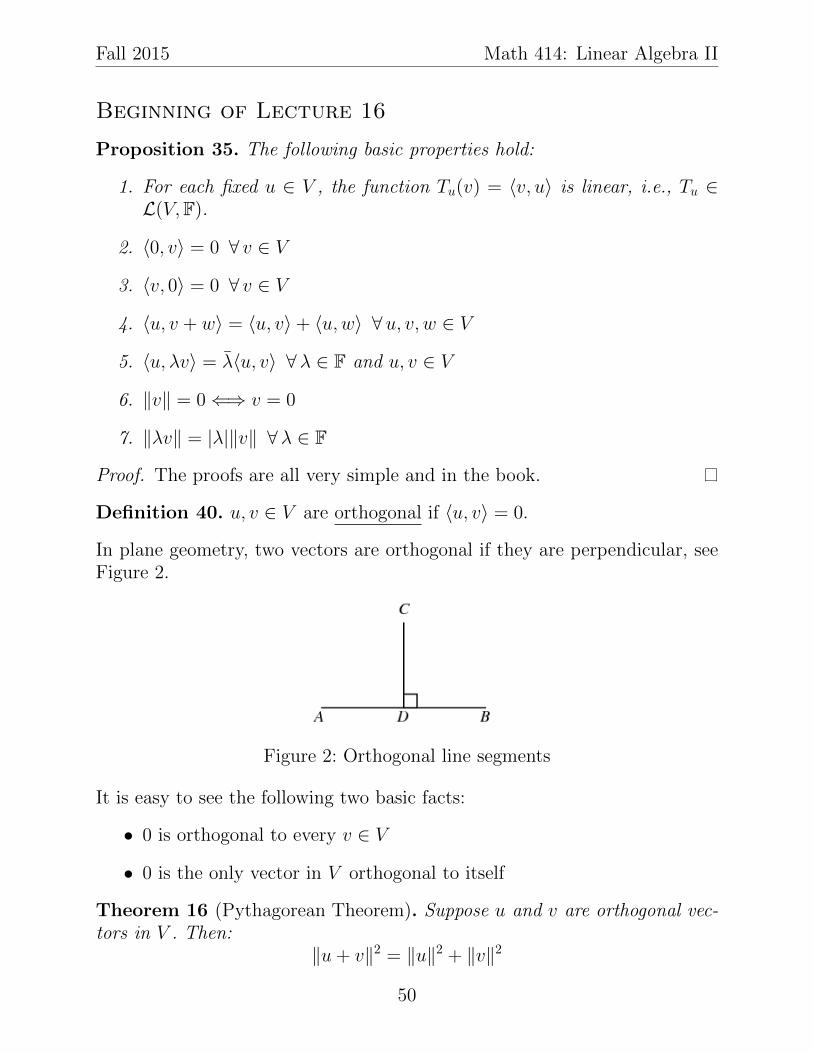
Definition 40. u, v ∈ V are orthogonal if 〈u, v〉 = 0.

In plane geometry, two vectors are orthogonal if they are perpendicular, seeFigure 2.

Figure 2: Orthogonal line segments

It is easy to see the following two basic facts:

• 0 is orthogonal to every v ∈ V

• 0 is the only vector in V orthogonal to itself

Theorem 16 (Pythagorean Theorem). Suppose u and v are orthogonal vec-tors in V . Then:

‖u+ v‖2 = ‖u‖2 + ‖v‖2

50


Figure 3: Orthogonal decomposition of u

Proof.

‖u+ v‖2 = 〈u+ v, u+ v〉= 〈u, u〉+ 〈u, v〉+ 〈v, u〉+ 〈v, v〉= ‖u‖2 + ‖v‖2

Now consider the following problem: Suppose u, v ∈ V with v 6= 0. We wantto write u as:

u = cv + w, 〈v, w〉 = 0

From the book, we have the picture in Figure 3. The question is, what are cand w?

First write u as:u = cv + (u− cv)

We need to choose c such that:

0 = 〈u− cv, v〉 = 〈u, v〉 − c‖v‖2 ⇒ c = 〈u, v〉/‖v‖2

We summarize this in the following proposition:

Proposition 36. Suppose u, v ∈ V with v 6= 0. Set:

c =〈u, v〉‖v‖2

and w = u− 〈u, v〉‖v‖2

v.

51


Then:〈w, v〉 = 0 and u = cv + w

Theorem 17 (Cauchy-Schwarz Inequality). Suppose u, v ∈ V . Then:

|〈u, v〉| ≤ ‖u‖‖v‖

Furthermore,|〈u, v〉| = ‖u‖‖v‖ ⇐⇒ u = cv

Proof. If v = 0 then both sides are zero. Thus assume v 6= 0, and apply theorthogonal decomposition to u:

u =〈u, v〉‖v‖2

+ w, 〈v, w〉 = 0

By the Pythagorean Theorem:

‖u‖2 =

∥∥∥∥〈u, v〉‖v‖2v

∥∥∥∥2

+ ‖w‖2

=|〈u, v〉|2

‖v‖2+ ‖w‖2

≥ |〈u, v〉|2

‖v‖2

Now multiply both sides by ‖v‖2.

For the second part, we see from the above proof that equality holds if andonly if w = 0. But then:

w = u− 〈u, v〉‖v‖2

v = 0⇐⇒ u =〈u, v〉‖v‖2

v

The Cauchy-Schwarz Inequality is one of the most important, and most used,inequalities in all of mathematics! Lets now use it to prove the triangle in-equality for general inner product spaces; Figure 6 gives the plane geometryintuition.

52


Figure 4: The triangle inequality for R2

Figure 5: Parallelogram equality in R2

Theorem 18 (Triangle Inequality). Suppose u, v ∈ V . Then:

‖u+ v‖ ≤ ‖u‖+ ‖v‖,

with equality if and only if u = cv for c ≥ 0.

The next result is the Parallelogram Equality, which also has a geometricinterpretation in R2; see Figure 7.

Proposition 37. Suppose u, v ∈ V . Then:

‖u+ v‖2 + ‖u− v‖2 = 2(‖u‖2 + ‖v‖2)

End of Lecture 16

53


Lecture 17: Midterm 1

Chapters 1-5

Lecture 18: Review of Midterm 1 Solutions

54



Theorem 19 (Triangle Inequality). Suppose u, v ∈ V . Then:

‖u+ v‖ ≤ ‖u‖+ ‖v‖,

with equality if and only if u = cv for c ≥ 0.

Proof. For the first part:

‖u+ v‖2 = 〈u+ v, u+ v〉= 〈u, u〉+ 〈v, v〉+ 〈u, v〉+ 〈v, u〉= 〈u, u〉+ 〈v, v〉+ 〈u, v〉+ 〈u, v〉= ‖u‖2 + ‖v‖2 + 2Re〈u, v〉≤ ‖u‖2 + ‖v‖2 + 2|〈u, v〉|≤ ‖u‖2 + ‖v‖2 + 2‖u‖‖v‖ [Cauchy-Schwarz]

= (‖u‖+ ‖v‖)2

The proof above shows that equality holds if and only if:

1. Re〈u, v〉 = |〈u, v〉|, and

2. |〈u, v〉| = ‖u‖‖v‖From the Cauchy-Schwartz inequality, we know #2 holds if and only if u = cvfor some c ∈ F. For #1, consider an arbitrary λ = a+ ib ∈ C, where a, b ∈ R.Then Reλ = a and |λ| =

√a2 + b2, so Reλ = |λ| if and only if λ = a ≥ 0.

Thus #1 holds if and only if 〈u, v〉 ≥ 0, which combined with u = cv, impliesthat equality holds if and only if c ≥ 0.

The next result is the Parallelogram Equality, which also has a geometricinterpretation in R2; see Figure 7.

Proposition 38. Suppose u, v ∈ V . Then:

‖u+ v‖2 + ‖u− v‖2 = 2(‖u‖2 + ‖v‖2)

Proof. Simply compute:

‖u+ v‖2 + ‖u− v‖2 = 〈u+ v, u+ v〉+ 〈u− v, u− v〉= ‖u‖2 + ‖v‖2 + 〈u, v〉+ 〈v, u〉+ ‖u‖2 + ‖v‖2 − 〈u, v〉+ 〈v, u〉= 2(‖u‖2 + ‖v‖2)

55


Figure 6: The triangle inequality for R2

Figure 7: Parallelogram equality in R2

6.B Orthonormal Bases

Definition 41. A list of vectors e1, . . . , em ∈ V is orthonormal if

〈ej, ek〉 =

{1 if j = k [norm 1]0 if j 6= k [orthogonal]

}= δ(j − k),

whereδ : Z→ C, δ(0) = 1 and δ(n) = 0, ∀n 6= 0.

Examples:

1. The standard basis in Fn

2. Recalls the vector space V = {f : ZN → C}, where ZN = {0, . . . , N −1}, and the Fourier basis:

ek : ZN → C, ek(n) =1√Ne2πikn/N .

Define an inner product on this vector space:

〈f, g〉 =N−1∑n=0

f(n)g(n)

56


Now V is an inner product space and e0, . . . , eN−1 is an orthonormallist. We can verify this:

〈ej, ek〉 =N−1∑n=0

ej(n)ek(n)

=1

N

N−1∑n=0

e2πijn/Ne−2πikn/N

=1

N

N−1∑n=0

e2πi(j−k)n/N

=

1N

∑N−1n=0 1 = 1

N ·N = 1 if j = k

1N ·

1−(e2πi(j−k)/N )N

1−e2πi(j−k)/N = 1N ·

1−e2πi(j−k)1−e2πi(j−k)/N = 1

N ·1−1

1−e2πi(j−k)/N = 0 if j 6= k

Since e0, . . . , eN−1 is also a basis, we call it an orthonormal basis.

Definition 42. An orthonormal basis of V is an orthonormal list of vectorsin V that is also a basis of V .

End of Lecture 19

57



Definition 43. An orthonormal basis of V is an orthonormal list of vectorsin V that is also a basis of V .

Orthonormal lists and bases are very convenient! For example:

Proposition 39. If e1, . . . , em is an orthonormal list of vectors in V , then:

‖a1e1 + · · ·+ amem‖2 = |a1|2 + · · ·+ |am|2, ∀ a1, . . . , am ∈ F.

Proof. Expand the left hand side:∥∥∥∥∥m∑k=1

akek

∥∥∥∥∥2

=m∑j=1

m∑k=1

〈ajej, akek〉

=m∑j=1

m∑k=1

ajak〈ej, ek〉

=m∑j=1

m∑k=1

ajakδ(j − k)

=m∑k=1

|ak|2

Corollary 6 (Important!). Every orthonormal list of vectors is linearly in-dependent.

Proof. Suppose e1, . . . , em is an orthonormal list of vectors in V and a1, . . . , am ∈F are such that:

m∑k=1

akek = 0.

Then by the previous proposition, |a1|2 + · · ·+ |am|2 = 0, which means ak = 0for all k since |ak|2 ≥ 0. Thus e1, . . . , em are linearly independent.

Proposition 40. If dimV = n and e1, . . . , en ∈ V is an orthonormal list ofvectors, then e1, . . . , em is an orthonormal basis.

Proof. By the previous corollary such a list must be linearly independent,and since n = dimV it then must be a basis.

58


In general, given a basis v1, . . . , vn of V and a vector v ∈ V , we know thereexists a1, . . . , an ∈ F such that

v = a1v1 + · · ·+ anvn

However, computing a1, . . . , an can be difficult. If we use an orthonormal basisthough, the calculation becomes very easy!

Theorem 20. Suppose e1, . . . , en is an orthonormal basis of V and v ∈ V .Then:

v =n∑k=1

〈v, ek〉︸︷︷︸ak

ek

and

‖v‖2 =n∑k=1

|〈v, ek〉|2

Proof. Because e1, . . . , en is a basis of V , there exists a1, . . . , an ∈ F such that

v =n∑k=1

akek

Now compute the inner product of both sides of the previous equation withej:

〈v, ej〉 = 〈n∑k=1

akek, ej〉 =n∑k=1

ak〈ek, ej〉 =n∑k=1

akδ(j − k) = aj

The second equation on ‖v‖2 now follows immediately from Proposition 39.

Since orthonormal bases are so useful, how do we go about finding them?The next algorithm shows how to turn any linearly independent list into anorthonormal list with the same span.

Theorem 21 (Gram-Schmidt). Suppose v1, . . . , vm ∈ V are linearly indepen-dent. Define:

e1 =v1

‖v1‖,

and then for k = 2, . . . ,m, define ek inductively by:

ek =vk −

∑k−1j=1〈vk, ej〉ej∥∥∥vk −∑k−1j=1〈vk, ej〉ej

∥∥∥ (13)

59


Then e1, . . . , em ∈ V is an orthonormal list of vectors such that:

span(v1, . . . , vk) = span(e1, . . . , ek), ∀ k = 1, . . . ,m.

Remark: Step two of the Gram-Schmidt algorithm is:

e2 =v2 − 〈v2, e1〉e1

‖v2 − 〈v2, e1〉e1‖=

1

‖v2 − 〈v2, e1〉e1‖·(v2 −

〈v2, v1〉‖v1‖2

v1

)which looks very similar to our orthogonal decomposition theorem from 6.A.The only difference is that e2 is normalized to have norm one. The idea ofGram-Schmidt is to iterate on this decomposition. Now for the proof:

Proof. Proof by induction on k. For k = 1, clearly span(v1) = span(e1), andso our base case holds.

Now suppose that for 1 < k < m we have

span(v1, . . . , vk−1) = span(e1, . . . , ek−1),

and let us consider e1, . . . , ek. First note that vk /∈ span(v1, . . . , vk−1) (be-cause they are linearly independent) and thus vk /∈ span(e1, . . . , ek−1). Thusdenominator of ek in (13) is not zero and so it is well defined. Clearly it hasnorm one, i.e., ‖ek‖ = 1.

Now let 1 ≤ j < k. Then:

〈ek, ej〉 =

⟨vk −

∑k−1j=1〈vk, ej〉ej∥∥∥vk −∑k−1j=1〈vk, ej〉ej

∥∥∥ , ek⟩

=〈vk, ej〉 − 〈vk, ej〉∥∥∥vk −∑k−1

j=1〈vk, ej〉ej∥∥∥

= 0

Thus e1, . . . , ek is an orthonormal list.

By the definition of ek, we have:

vk =

∥∥∥∥∥vk −k−1∑j=1

〈vk, ej〉ej

∥∥∥∥∥ ek +k−1∑j=1

〈vk, ej〉ej

60


and so vk ∈ span(e1, . . . , ek). Thus by the inductive hypothesis,

span(v1, . . . , vk) ⊂ span(e1, . . . , ek).

But both lists v1, . . . , vk and e1, . . . , ek are linearly independent, and thusboth subspaces have dimension k. Therefore they must be equal.

End of Lecture 20

61



Example: Let’s use Gram-Schmidt find an orthonormal basis of P2([−1, 1];R)with the inner product:

〈p, q〉 =

∫ 1

−1

p(x)q(x) dx.

Let’s start with the standard basis 1, x, x2 which is linearly independent butnot orthonormal. We start by computing:

‖1‖2 =

∫ 1

−1

12 dx = 2

Thus:e1 = 1/‖1‖ = 1/

√2

Now we need to compute e2. So we compute:

x− 〈x, e1〉e1 = x−(∫ 1

−1

x1√2dx

)1√2

= x

and also:

‖x− 〈x, e1〉e1‖2 = ‖x‖2 =

∫ 1

−1

x2 dx =2

3.

Thus:

e2 =x− 〈x, e1〉e1

‖x− 〈x, e1〉e1‖=

√3

2x

Now we need to compute e3. We have:

x2 − 〈x2, e1〉e1 − 〈x2, e2〉e2 = x2 −(∫ 1

−1

x2 1√2dx

)1√2−

(∫ 1

−1

x2

√3

2x dx

)√3

2x

= x2 − 1

3

62


and also

‖x2 − 〈x2, e1〉e1 − 〈x2, e2〉e2‖2 =

∥∥∥∥x2 − 1

3

∥∥∥∥2

=

∫ 1

−1

(x2 − 1

3

)2

dx

=

∫ 1

−1

(x4 − 2

3x2 +

1

9

)dx =

8

45.

Hence:

e3 =

√45

8

(x2 − 1

3

).

Thus

B =1√2,

√3

2x,

√45

8(x2 − 1/3)

is an orthonormal basis for P2([−1, 1];R).

The Gram-Schmidt algorithm can be used to prove several useful facts, whichwe do now.

Proposition 41. Every finite dimensional inner product space has an or-thonormal basis.

Proof. Choose any basis of V and apply the Gram-Schmidt algorithm to itto get an orthonormal basis.

Just as we can extend any linearly independent list to a basis, we can alsoextend any orthonormal list to an orthonormal basis.

Proposition 42. If V is a finite dimensional inner product space, then everylist of orthonormal vectors in V can be extended to an orthonormal basis ofV .

Proof. Let e1, . . . , em ∈ V be an orthonormal list. Since they are linearlyindependent, we can extend them to a basis:

e1, . . . , em, v1, . . . , vn

63


Now apply the Gram-Schmidt algorithm to this basis. Since e1, . . . , em areorthonormal, as you can verify the Gram-Schmidt algorithm will leave themunchanged. Thus we get an orthonormal basis of the form:

e1, . . . , em, f1, . . . , fn

Now we return to upper-triangular matrices. Recall that we previously showedthat if V is a finite dimensional complex vector space, then for each T ∈ L(V )there is a basis B such thatM(T ;B) is upper triangular. When V is an innerproduct space, we would like to take B to be an orthonormal basis.

Proposition 43. Suppose T ∈ L(V ). If M(T ;B) is upper triangular forsome basis B, then there exists an orthonormal basis B′ such that M(T ;B′)is upper triangular.

Proof. Suppose M(T ;B) is upper triangular and B = v1, . . . , vn. Then Uk =span(v1, . . . , vk) is invariant under T for each k = 1, . . . , n.

Apply the Gram-Schmidt algorithm to B, producing an orthonormal basisB′ = e1, . . . , en. We claim B′ is the desired basis. Indeed,

span(e1, . . . , ek) = span(v1, . . . , vk) = Uk, ∀ k = 1, . . . , n.

Therefore span(e1, . . . , ek) is invariant under T for each k = 1, . . . , n. ThusM(T ;B′) is upper triangular.

Remark: The above proposition holds for any inner product space and op-erator T for which there exists some basis B such that M(T ;B) is uppertriangular. In particular, V can be a real vector space, if such a B exists. Ofcourse when V is a complex vector space, we can guarantee the result...

Theorem 22 (Schur’s Theorem). If V is a finite dimensional complex innerproduct space and T ∈ L(V ), then there exists an orthonormal basis B′ suchthat M(T ;B′) is upper triangular.

Proof. Since V is a finite dimensional complex vector space, there exists abasis B such thatM(T ;B) is upper triangular. Now apply the previous propo-sition.

End of Lecture 21

64



Definition 44. A function ϕ is a linear functional on V if ϕ ∈ L(V,F).

Examples:

• Fix an arbitrary u ∈ V . Then:

ϕ : V → Fv 7→ ϕ(v) = 〈v, u〉

is a linear functional on V .

• Fix an arbitrary continuous function f ∈ C([−1, 1];R). Then:

ϕ : P2([−1, 1];R)→ R

p 7→ ϕ(p) =

∫ 1

−1

p(x)f(x) dx

is a linear functional on P([−1, 1];R).

Remark: It is tempting to write ϕ(p) = 〈p, f〉, but we may not havef ∈ P2([−1, 1];R). For example, f(x) = cos(x) or f(x) = ex, and so〈p, f〉 does not necessarily make sense. Thus the next result is quiteremarkable...

Theorem 23 (Riesz Representation Theorem). Suppose V is finite-dimensionaland ϕ ∈ L(V,F). Then there is a unique vector u ∈ V such that

ϕ(v) = 〈v, u〉, ∀v ∈ V

Proof. First we show that there exists a u ∈ V such that ϕ(v) = 〈v, u〉, thenwe show that u is unique. Let e1, . . . , en be an orthonormal basis of V . Then:

ϕ(v) = ϕ

(n∑k=1

〈v, ek〉ek

)

=n∑k=1

〈v, ek〉ϕ(ek)

= 〈v,n∑k=1

ϕ(ek)ek〉

65


Thus setting:

u =n∑k=1

ϕ(ek)ek

we have ϕ(v) = 〈v, u〉 for all v ∈ V .

Now we prove that u is unique. Suppose u1, u2 ∈ V such that

ϕ(v) = 〈v, u1〉 = 〈v, u2〉, ∀ v ∈ V

Then:0 = 〈v, u1〉 − 〈v, u2〉 = 〈v, u1 − u2〉, ∀ v ∈ V

Taking v = u1 − u2 implies ‖u1 − u2‖2 = 0 which implies that u1 − u2 = 0and so u1 = u2. Therefore u is unique.

Remark (con’t): Returning to the example above, even if f ∈ C([−1, 1];R)

and f /∈ P2([−1, 1];R), there still exists a unique q ∈ P2([−1, 1];R) such that:

ϕ(p) =

∫ 1

−1

p(x)f(x) dx =

∫ 1

−1

p(x)q(x) dx = 〈p, q〉, ∀ p ∈ P2([−1, 1];R).

Furthermore, we can compute what q is by selecting an orthonormal basise1, e2, e3 for P2([−1, 1];R) (like the one we computed earlier) and using theformula:

q = ϕ(e1)e1 + ϕ(e2)e2 + ϕ(e3)e3

This works in general.

End of Lecture 22

66



6.C Orthogonal Complements and Minimization Prob-

lems

Definition 45. If U ⊂ V , then the orthogonal complement of U is:

U⊥ = {v ∈ V : 〈v, u〉 = 0, ∀u ∈ U}

Geometrical Examples:

• If U is a line in V = R2, then U⊥ is the line orthogonal U that passesthrough the origin.

• If U is a line in V = R3, then U⊥ is the plane orthogonal to U thatcontains the origin.

• If U is a plane in V = R3, then U⊥ is the line orthogonal to U thatpasses through the origin.

Proposition 44. The following are basic properties of the orthogonal com-plement:

1. If U ⊂ V , then U⊥ is a subspace of V

2. {0}⊥ = V

3. V ⊥ = {0}

4. If U ⊂ V , then U ∩U⊥ ⊂ {0}. If U is a subspace of V , then U ∩U⊥ ={0}.

5. If U ⊂ V and W ⊂ V ad U ⊂ W , then W⊥ ⊂ U⊥

Proof. We go through the list:

1. We need to show U⊥ contains 0, is closed under addition and scalarmultiplication.

• Clearly 〈0, u〉 = 0 ∀u ∈ U , thus 0 ∈ U⊥.

• Now suppose v, w ∈ U⊥. If u ∈ U , then:

〈v + w, u〉 = 〈v, u〉+ 〈w, u〉 = 0 + 0 = 0 =⇒ v + w ∈ U⊥

67


• Suppose λ ∈ F and v ∈ U⊥. If u ∈ U , then

〈λv, u〉 = λ〈v, u〉 = λ · 0 = 0 =⇒ λv ∈ U⊥

2. 〈v, 0〉 = 0 ∀ v ∈ V =⇒ v ∈ {0}⊥, so {0}⊥ = V

3. Suppose v ∈ V ⊥. Then 〈v, v〉 = 0 =⇒ v = 0. Thus V ⊥ = {0}.

4. Suppose U ⊂ V and v ∈ U ∩ U⊥. Then we must have 〈v, v〉 = 0 =⇒v = 0, and so U ∩ U⊥ ⊂ {0}. If U is a subspace of V , then 0 ∈ U andby above 0 ∈ U⊥, so U ∩ U⊥ = {0}.

5. This is clear.

Recall early on we proved that if U is a subspace of V , then there exists asecond subspace W of V such that V = U ⊕W . We now show that we cantake W = U⊥.

Proposition 45. If U is a finite dimensional subspace of V , then

V = U ⊕ U⊥

Proof. From the previous proposition we know that U ∩U⊥ = {0}, so we justneed to show that U + U⊥ = V . Let v ∈ V and let e1, . . . , em be an ONB ofU . Clearly then:

v =m∑k=1

〈v, ek〉ek︸︷︷︸u∈U

+ v −m∑k=1

〈v, ek〉ek︸︷︷︸w

We want to show w ∈ U⊥. But this is clear since:

∀ k = 1, . . . ,m, 〈w, ek〉 = 〈v, ek〉 − 〈v, ek〉 = 0 =⇒ w ∈ U⊥

Corollary 7. If V is finite dimensional and U is a subspace of V , then:

dimU⊥ = dimV − dimU

Proposition 46. If U is a finite dimensional subspace of V , then

U = (U⊥)⊥

68


Proof. We prove this in two parts:

• First we show that U ⊂ (U⊥)⊥. Suppose u ∈ U . Then by definition ofU⊥,

〈v, u〉 = 0 = 〈u, v〉, ∀ v ∈ U⊥

But the above also implies that u ∈ (U⊥)⊥ since

(U⊥)⊥ = {w ∈ V : 〈w, v〉 = 0, ∀ v ∈ U⊥}

• Now we show that (U⊥)⊥ ⊂ U . Suppose that v ∈ (U⊥)⊥. v ∈ V so wecan write it as:

v = u+ w, u ∈ U, w ∈ U⊥ =⇒ v − u = w ∈ U⊥

But by the above, we also have u ∈ U ⊂ (U⊥)⊥ and so:

v − u ∈ (U⊥)⊥ ⇒ v − u ∈ U⊥ ∩ (U⊥)⊥ ⇒ v − u = 0⇒ v = u⇒ v ∈ U

End of Lecture 23

69



Now we use the fact that V = U ⊕U⊥ to define the orthogonal projection ofV onto U .

Definition 46. Suppose U is a finite dimensional subspace of V .The orthogonal projection of V onto U is the operator PU ∈ L(V ) definedas:

PUv = u, where v = u+ w, u ∈ U, w ∈ U⊥

Remark: Since the decomposition v = u+w ∈ U ⊕U⊥ is unique, the orthog-onal projection PU is well defined.

Example: Recall from earlier we have: If u, v ∈ V and u 6= 0, then

v = cu+ w, 〈u,w〉 = 0, c =〈v, u〉‖u‖2

Thus if U = span(u), then

PUv = cu =〈v, u〉‖u‖2

u

More generally, if U is an arbitrary finite dimensional subspace of V ande1, . . . , em is an ONB for U , then:

PUv =m∑k=1

〈v, ek〉ek (14)

This is just one of many properties of PU :

Proposition 47. If U is a finite dimensional subspace of V and v ∈ V , then:

1. PU ∈ L(V )

2. PUu = u ∀u ∈ U

3. PUw = 0 ∀w ∈ U⊥

4. rangePU = U

5. nullPU = U⊥

70


6. v − PUv ∈ U⊥

7. P 2U = PU

8. ‖PUv‖ ≤ ‖v‖

Proof. We prove each part:

1. This follows from (14) and the linearity of the inner product in the firstargument.

2. If u ∈ U , then u = u+ 0 ∈ U ⊕ U⊥, and thus PUu = u.

3. If w ∈ U⊥, then w = 0 + w ∈ U ⊕ U⊥, and thus PUw = 0.

4. This is clear

5. Part 3 implies that U⊥ ⊂ nullPU . Now suppose that v ∈ nullPU , i.e.,PUv = 0. Then if v = u + w ∈ U ⊕ U⊥, we must have PUv = u = 0,which implies that v = 0 + w = w ∈ U⊥ and so nullPU ⊂ U⊥.

6. If v = u+ w ∈ U ⊕ U⊥, then:

v − PUv = (u+ w)− u = w ∈ U⊥

7. If v = u+ w ∈ U ⊕ U⊥ then:

(P 2U)v = PU(PUv) = PUu = u = PUv

8. If v = u+ w ∈ U ⊕ U⊥ then:

‖PUv‖2 = ‖u‖2 ≤ ‖u‖2 + ‖w‖2 = ‖v‖2

We now turn to a very important minimization problem: Given a subspaceU of V and a point v ∈ V , find a point u0 ∈ U such that ‖v− u0‖ is as smallas possible. In other words, find u0 ∈ U such that:

‖v − u0‖ = minu∈U‖v − u‖ ⇐⇒ ‖v − u0‖ ≤ ‖v − u‖, ∀u ∈ U

In fact the orthogonal projection gives the solution!

71


Theorem 24. Suppose U is a finite dimensional subspace of V , v ∈ V , andu ∈ U . Then:

‖v − PUv‖ ≤ ‖v − u‖.Furthermore,

‖v − PUv‖ = ‖v − u‖ ⇐⇒ u = PUv

Proof. We have:

‖v − PUv‖2 ≤ ‖ v − PUv︸︷︷︸∈U⊥

‖2 + ‖PUv − u︸︷︷︸∈U

‖2

= ‖(v − PUv) + (PUv − u)‖2

= ‖v − u‖2

The inequality is an equality if and only if:

‖v − PUv‖ = ‖v − u‖ ⇔ ‖v − PUv‖2 = ‖v − PUv‖2 + ‖PUv − u‖2

⇔ ‖PUv − u‖2 = 0

⇔ PUv = u

Please read the very interesting Example 6.58 in the book.

End of Lecture 24

72



7 Operators on Inner Product Spaces

We now explore the structure of operators on inner product spaces, whichwe have been building towards for quite a while now. This will lead to someof the most important results in all of Linear Algebra. In particular, we willcompletely characterize those operators that are diagonalizable, giving us acomplete solution to the questions we asked at the beginning of Chapter 5.

Notation: V and W are inner product spaces over the same field F. Some-times we will write 〈·, ·〉V for the inner product on V and 〈·, ·〉W for the innerproduct on W .

7.A Self-Adjoint and Normal Operators

Definition 47. Suppose T ∈ L(V,W ). The adjoint of T is the functionT ∗ : W → V such that:

〈Tv, w〉W = 〈v, T ∗w〉V , ∀ v ∈ V, ∀w ∈ W

Warmup: Show the T ∗ is well-defined.

Solution: Fix T ∈ L(V,W ) and w ∈ W and consider the linear functionalϕ ∈ L(V,F) defined as:

ϕ(v) = 〈Tv, w〉By the Riesz Representation Theorem, there exists a unique vector u ∈ Vsuch that:

〈Tv, w〉 = ϕ(v) = 〈v, u〉Define T ∗w := u.

Example: Consider the vector space:

V = {f ∈ C∞([0, 1];R) : f (k)(0) = f (k)(1) ∀ k = 0, 1, 2, . . .}

Define the inner product on V as:

〈f, g〉 =

∫ 1

0

f(x)g(x) dx, f, g ∈ V

73


Let T ∈ L(V ) be the differentiation operator, i.e., T = D where

Df = f ′

Let’s compute the adjoint of D using integration by parts:

〈Df, g〉 =

∫ 1

0

Df(x)g(x) dx

=

∫ 1

0

f ′(x)g(x) dx

= f(x)g(x)|x=1x=0 −

∫ 1

0

f(x)g′(x) dx

= 0−∫ 1

0

f(x)g′(x) dx

=

∫ 1

0

f(x) · (−Dg(x)) dx

= 〈f,−Dg〉

Thus, D∗ = −D.

We have used this technique before, but it will be especially useful whendealing with adjoints and so we write it down here:

Lemma 2. Let u,w ∈ V . If:

〈v, u〉 = 〈v, w〉, ∀ v ∈ V,

then u = w.

Proof. Indeed,

〈v, u〉 = 〈v, w〉, ∀ v ∈ V =⇒ 〈v, u− w〉 = 0, ∀ v ∈ V

Since it is true for all v ∈ V , we can take v = u− w and we then have:

〈u− w, u− w〉 = 0 =⇒ ‖u− w‖2 = 0 =⇒ u− w = 0 =⇒ u = w

Proposition 48. If T ∈ L(V,W ), then T ∗ ∈ L(W,V )

74


Proof. Need to show additivity and homogeneity of T ∗. Let w1, w2 ∈ W andv ∈ V :

〈v, T ∗(w1 + w2)〉V = 〈Tv, w1 + w2〉W= 〈Tv, w1〉W + 〈Tv, w2〉W= 〈v, T ∗w1〉V + 〈v, T ∗w1〉V= 〈v, T ∗w1 + T ∗w2〉V

Therefore T ∗(w1 + w2) = T ∗w1 + T ∗w2.

Now let w ∈ W , λ ∈ F, and v ∈ V :

〈v, T ∗(λw)〉V = 〈Tv, λw〉W= λ〈Tv, w〉W= λ〈v, T ∗w〉V= 〈v, λT ∗w〉V

and so T ∗(λw) = λT ∗w

Proposition 49. The following properties of the adjoint hold:

1. (S + T )∗ = S∗ + T ∗, ∀S, T ∈ L(V,W )

2. (λT )∗ = λT ∗, ∀λ ∈ F, ∀T ∈ L(V,W )

3. (T ∗)∗ = T, ∀T ∈ L(V,W )

4. I∗ = I, where I ∈ L(V ) is the identity operator, i.e., Iv = v ∀v ∈ V

5. (ST )∗ = T ∗S∗, ∀T ∈ L(V,W ), ∀S ∈ L(W,U)

Proof. The proofs of #1 and #2 are very similar to the proof that T ∗ islinear. The proof of #4 is also quite easy.

To prove #3, let v ∈ V and w ∈ W ,

〈w, (T ∗)∗v〉 = 〈T ∗w, v〉 = 〈v, T ∗w〉 = 〈Tv, w〉 = 〈w, Tv〉

To prove #5, let v ∈ V and u ∈ U ,

〈v, (ST )∗u〉 = 〈STv, u〉 = 〈Tv, S∗u〉 = 〈v, T ∗S∗u〉

End of Lecture 25

75



The null space and range of T are related to the null space and range ofT ∗ through the orthogonal complement, as we now prove.

Proposition 50. If T ∈ L(V,W ), then:

1. nullT ∗ = (rangeT )⊥

2. rangeT ∗ = (nullT )⊥

3. nullT = (rangeT ∗)⊥

4. rangeT = (nullT ∗)⊥

Proof. We prove #1 first:

w ∈ nullT ∗ ⇐⇒ T ∗w = 0

⇐⇒ 〈v, T ∗w〉 = 0, ∀ v ∈ V⇐⇒ 〈Tv, w〉 = 0, ∀ v ∈ V⇐⇒ w ∈ (rangeT )⊥

Thus nullT ∗ = (rangeT )⊥.

The rest now follow easily. Indeed, taking the orthogonal complement of bothsides of #1 gives #4. Replacing T with T ∗ in #1 gives #3, and in number#4 gives #2.

We now relate the adjoint to matrices.

Definition 48. The conjugate transpose of an m×n matrix A ∈ Fm,n is the

n×m matrix A† ∈ Fn,m defined as:

A†j,k = Ak,j, ∀ j = 1, . . . , n, k = 1, . . . ,m

Proposition 51. Let T ∈ L(V,W ), BV = e1, . . . , en be an ONB of V , andBW = f1, . . . , fm be an ONB of W (note: they must be orthonormal!!). Then:

M(T ∗;BW ,BV ) =M(T ;BV ,BW )†

76


Proof. Let A =M(T ;BV ,BW ). Recall that Aj,k is defined by writing Tek asa linear combinations of f1, . . . , fm:

Tek =m∑j=1

Aj,kfj =m∑j=1

〈Tek, fj〉Wfj =⇒ Aj,k = 〈Tek, fj〉W

where the second equality follows since BW is an ONB.

Now let B =M(T ∗;BW ,BV ). Then B is defined as:

T ∗fk =n∑j=1

Bj,kej =n∑j=1

〈T ∗fk, ej〉V ej =⇒ Bj,k = 〈T ∗fk, ej〉V

But then:

Bj,k = 〈T ∗fk, ej〉 = 〈ej, T ∗fk〉 = 〈Tej, fk〉 = Ak,j = A†j,k

Now we focus in on operators T ∈ L(V ), where V is an inner product space.We shall be particularly interested in the following operators.

Definition 49. An operator T ∈ L(V ) is self-adjoint if T = T ∗, i.e.,

〈Tv, w〉 = 〈v, Tw〉, ∀ v, w ∈ V

Remark: The previous proposition shows that for a general T ∈ L(V ), ifB is an ONB for V , then M(T ∗;B) = M(T ;B)†. But if T is self-adjoint,then T = T ∗ and so M(T ;B) = M(T ∗;B) = M(T ;B)†, which implies thatM(T ;B) is symmetric and real valued.

Proposition 52. The eigenvalues of self-adjoint operators are real valued(even when F = C).

Proof. Let T ∈ L(V ) be self-adjoint, λ ∈ F and eigenvalue of T , and v ∈ Va corresponding nonzero eigenvector so that Tv = λv. Then:

λ‖v‖2 = 〈λv, v〉 = 〈Tv, v〉 = 〈v, Tv〉 = 〈v, λv〉 = λ‖v‖2 ⇒ λ = λ⇒ λ ∈ R

77


Proposition 53. Let V be a complex inner product space and T ∈ L(V ).

If 〈Tv, v〉 = 0, ∀ v ∈ V, then T = 0

Proof. Suppose 〈Tv, v〉 = 0, ∀ v ∈ V . Let u,w ∈ V and consider the cleverrewriting of 〈Tu,w〉:

〈Tu,w〉 =1

4〈T (u+ w), u+ w︸︷︷︸

v1

〉 − 1

4〈T (u− w), u− w︸︷︷︸

v2

〉

+1

4〈T (u+ iw), u+ iw︸︷︷︸

v3

〉i− 1

4〈T (u− iw), u− iw︸︷︷︸

v4

〉i

=1

4(〈Tv1, v1〉+ 〈Tv2, v2〉+ 〈Tv3, v3〉i+ 〈Tv4, v4〉i)

= 0

Thus 〈Tu,w〉 = 0, ∀u,w ∈ V . Taking w = Tu, we get ‖Tu‖2 = 0, ∀u ∈ V ,which implies that Tu = 0 for all u ∈ V , and so T = 0.

Remark: False if F = R. Take V = R2 and T to be a 90-degree rotation.

Proposition 54. Suppose V is a complex inner product space and T ∈ L(V ).Then:

T is self-adjoint⇐⇒ 〈Tv, v〉 ∈ R, ∀ v ∈ V

Proof. Let v ∈ V , then:

〈Tv, v〉−〈Tv, v〉 = 〈Tv, v〉−〈v, Tv〉 = 〈Tv, v−〈T ∗v, v〉 = 〈(T−T ∗)v, v〉 (15)

If 〈Tv, v〉 ∈ R, then by (15):

0 = 〈(T − T ∗)v, v〉 =⇒ T − T ∗ = 0 [by previous Proposition] =⇒ T = T ∗

Conversely, if T is self=adjoint then (15) also implies:

〈Tv, v〉 − 〈Tv, v〉 = 0 =⇒ 〈Tv, v〉 = 〈Tv, v〉 =⇒ 〈Tv, v〉 ∈ R

Remark: Also false if F = R since 〈Tv, v〉 ∈ R for all T ∈ L(V ), includingthose that are not self-adjoint.

End of Lecture 26

78



Proposition 55. If T is self-adjoint and 〈Tv, v〉 = 0 for all v ∈ V , thenT = 0 (even if F = R).

Proof. If F = C then we already proved this. So assume that F = R, andsuppose that T is self-adjoint and 〈Tv, v〉 = 0 for all v ∈ V . Let u,w ∈ V ;then:

〈T (u+ w), u+ w〉 − 〈T (u− w), u− w〉 =

= 〈Tu, u〉+ 〈Tu,w〉+ 〈Tw, u〉+ 〈Tw,w〉 − 〈Tu, u〉+ 〈Tu,w〉+ 〈Tw, u〉 − 〈Tw,w〉= 2〈Tu,w〉+ 2〈Tw, u〉= 2〈Tu,w〉+ 2〈u, Tw〉 [F = R]

= 4〈Tu,w〉 [T = T ∗]

Thus, let v1 = u+ w and v2 = u− w:

〈Tu,w〉 =1

4(〈Tv1, v1〉+ 〈Tv2, v2〉) = 0, ∀u,w ∈ V =⇒ T = 0

Self-adjoint operators are a subset of the following class of important opera-tors.

Definition 50. T ∈ L(V ) is normal if

TT ∗ = T ∗T

Example: Recall the vector space:

V = {f ∈ C∞([0, 1];R) : f (k)(0) = f (k)(1), ∀ k = 0, 1, 2, . . .}

and the differentiation operator D ∈ L(V ),

Df = f ′

We showed that D∗ = −D. Thus D is not self adjoint, but

DD∗ = D(−D) = −D2 = (−D)D = D∗D

and so D is normal.

79


Proposition 56.

T is normal ⇐⇒ ‖Tv‖ = ‖T ∗v‖, ∀ v ∈ V

Proof. We have:

T is normal ⇐⇒ T ∗T − TT ∗ = 0

⇐⇒ 〈(T ∗T − TT ∗)v, v〉 = 0, ∀ v ∈ V (16)

⇐⇒ 〈T ∗Tv, v〉 = 〈TT ∗v, v〉, ∀ v ∈ V⇐⇒ ‖Tv‖2 = ‖T ∗v‖2, ∀ v ∈ V

where (16) follows from the previous Proposition since T ∗T − TT ∗ is self-adjoint.

Corollary 8. Suppose T ∈ L(V ) is normal. If v ∈ V is an eigenvector of Twith eigenvalue λ, then v is an eigenvector of T ∗ with eigenvalue λ.

Proof. T normal implies that T − λI is normal since:

(T − λI)(T − λI)∗ = (T − λI)(T ∗ − λI)

= TT ∗ − λT − λT ∗ + |λ|2I= T ∗T − λT ∗ − λT + |λ|2I= (T ∗ − λI)(T − λI)

= (T − λI)∗(T − λI)

Then by the previous Proposition:

0 = ‖(T − λI)v‖ = ‖(T − λI)∗v‖ = ‖(T ∗ − λI)v‖ =⇒ T ∗v = λv

Proposition 57. If T is normal, then the eigenvectors of T correspondingto distinct eigenvalues are orthogonal.

Proof. Let α, β be distinct eigenvalues of T with corresponding eigenvectorsu, v so that

Tu = αu and Tv = βv

From the previous Corollary we have T ∗v = βv. Thus:

(α− β)〈u, v〉 = α〈u, v〉 − β〈u, v〉 = 〈αu, v〉 − 〈u, βv〉 = 〈Tu, v〉 − 〈u, T ∗v〉 = 0

Since α 6= β, we must have 〈u, v〉 = 0.

80


7.B The Spectral Theorem

Two flavors, real and complex. As is often the case, the complex version is infact easier. So we start with that.

Complex Spectral Theorem

Theorem 25 (Complex Spectral Theorem). Suppose F = C and T ∈ L(V ).Then the following are equivalent:

1. T is normal

2. V has an ONB consisting of eigenvectors of T

3. T has a diagonal matrix with respect to some ONB of V

End of Lecture 27

81



Theorem 26 (Complex Spectral Theorem). Suppose F = C and T ∈ L(V ).Then the following are equivalent:

1. T is normal



Proof. We prove this in parts:

• (2) ⇐⇒ (3) follows from our work in Chapter 5.

• (3) =⇒ (1): Let B be an ONB such that M(T ;B) is diagonal. Then

M(T ∗;B) =M(T ;B)† =⇒M(T ∗;B) is diagonal

But then since diagonal matrices commute we have:

M(TT ∗;B) =M(T ;B)M(T ∗;B) =M(T ∗;B)M(T ;B) =M(T ∗T ;B)

=⇒ TT ∗ = T ∗T

since L(V ) and Cn,n are isomorphic under the linear mapM : L(V )→Cn,n.

• Now suppose that T is normal. By Schur’s Theorem there exists andONB B = e1, . . . , en such that M(T ;B) is upper triangular; write thematrix as:

M(T ;B) =

a1,1 · · · a1,n. . . ...

0 an,n

=⇒M(T ∗;B) =M(T ;B)† =

a1,1 0... . . .a1,n · · · an,n

We now show thatM(T ;B) is in fact a diagonal matrix. Indeed, becauseB is an ONB and T is normal:

‖Te1‖2 = |a1,1|2

‖Te1‖2 = ‖T ∗e1‖2 = |a1,1|2 + |a1,2|2 + · · ·+ |a1,n|2

=⇒ a1,2 = · · · = a1,n = 0

82


Now we also have:

‖Te2‖2 = |a1,2|2 + |a2,2|2 = 0 + |a2,2|2 = |a2,2|2

‖Te2‖2 = ‖T ∗e2‖2 = |a2,2|2 + |a2,3|2 + · · · |a2,n|2

=⇒ a2,3 = · · · = a2,n = 0

Continuing in this fashion we see that all off-diagonal entries must bezero.

Next week we will prove the Real Spectral Theorem:

Theorem 27 (Real Spectral Theorem). Suppose F = R and T ∈ L(V ). Thenthe following are equivalent:

1. T is self-adjoint



End of Lecture 28

83



Warmup: If we change F = R, where does the proof of the Complex SpectralTheorem fall apart?

Answer: To prove (1) =⇒ (3) we used Schur’s Theorem, which only appliesto complex vector spaces.

Real Spectral Theorem

We now aim to prove the Real Spectral Theorem:





The Real Spectral Theorem is harder to prove and as such we will first needsome preliminary results.

Consider the quadratic polynomial p ∈ P2(R):

p(x) = x2 + bx+ c, x, b, c ∈ R

Note the following:

If b2 < 4c, then x2 + bx+ c =

(x+

b

2

)2

+

(c− b2

4

)> 0, ∀x ∈ R

In particular p(x) > 0 so it has a multiplicative inverse for all x ∈ R, namelyp(x) · (1/p(x)) = 1. A similar type of reasoning leads to the following result.

Proposition 58. If T ∈ L(V ) is self-adjoint and b, c ∈ R satisfy b2 < 4c,then

p(T ) = T 2 + bT + cI

is invertible.

84


Proof. Let v ∈ V , v 6= 0. Then:

〈p(T )v, v〉 = 〈(T 2 + bT + cI)v, v〉= 〈T 2v, v〉+ b〈Tv, v〉+ c〈v, v〉= 〈Tv, Tv〉+ b〈Tv, v〉+ c‖v‖2

≥ ‖Tv‖2 − |b|‖Tv‖‖v‖+ c‖v‖2 [Cauchy-Schwarz]

=

(‖Tv‖ − |b|‖v‖

2

)2

+

(c− b2

4

)‖v‖2

> 0

Thus p(T )v 6= 0 =⇒ p(T ) is injective, and hence invertible.

End of Lecture 29

85



Proposition 59. If V 6= {0} and T ∈ L(V ) is self-adjoint, then T has aneigenvalue (even if F = R).

To prove this, we are going to need the following proposition from Chapter4 on polynomials.

Proposition 60. If p ∈ P(R) is a non-constant polynomial, then p has aunique factorization (except for re-ordering) of the form:

p(x) = c(x− λ1) · · · (x− λm)(x2 + b1x+ c1) · · · (x2 + bMx+ cM),

where

m+M ≥ 1

c ∈ R, c 6= 0

λ1, . . . , λm ∈ Rb1, . . . , bM ∈ Rc1, . . . , cM ∈ R

b2j < 4cj, ∀ j

Proof of Proposition 59. If F = C then T has an eigenvalue even if it is notself-adjoint (recall this from Chapter 5), so we can assume that F = R.

Let n = dimV and choose any v ∈ V with v 6= 0; then:

v, Tv, T 2v, . . . , T nv must be linearly dependent

Thus there exists a0, . . . , an ∈ R, not all zero, such that

0 =n∑k=0

akTkv

Define p(x) = a0 + a1x+ · · · anxn. Then using Proposition 60 we have:

p(x) = a0 + a1x+ · · ·+ anxn

= c(x− λ1) · · · (x− λm)(x2 + b1x+ c1) · · · (x2 + bMx+ cM)

86


Thus:

0 = a0v + a1Tv + · · · anT nv= (a0 + a1T + · · · anT n)v= c(T − λ1I) · · · (T − λmI)(T 2 + b1T + c1I) · · · (T 2 + bMT + cMI)v (17)

By Proposition 58, each T 2+bjT+cjI is invertible. Also, c 6= 0, so m > 0 sinceotherwise the RHS of (17) would be an invertible (hence injective) operatoracting a nonzero vector v, but the LHS is zero, and thus we would have acontradiction. Therefore,

0 = (T − λ1I) · · · (T − λmI)v =⇒ T − λjI is not injective for some j

=⇒ λj is an eigenvalue of T

Proposition 61. If T ∈ L(V ) is self-adjoint and U is an invariant subspaceof V under T , then:

1. U⊥ is invariant under T

2. T |U ∈ L(U) is self-adjoint

3. T |U⊥ ∈ L(U⊥) is self-adjoint

Proof. We prove each part:

1. Let v ∈ U⊥ and u ∈ U ; then:

〈Tv, u〉 = 〈v, Tu︸︷︷︸∈U〉 = 0, ∀u ∈ U =⇒ Tv ∈ U⊥

Thus U⊥ is invariant under T .

2. If u, v ∈ U , then:

〈(T |U)u, v〉 = 〈Tu, v〉 = 〈u, Tv〉 = 〈u, (T |U)v〉 =⇒ (T |U)∗ = T |U

3. Replace U with U⊥ in the proof of #2. This is valid because we havealready proved #1.

87






Proof. We prove (1) =⇒ (2) =⇒ (3) =⇒ (1) in parts:

• (2) =⇒ (3) is clear

• (3) =⇒ (1): Let B be an ONB such that M(T ;B) ∈ Rn,n is diagonal.ThenM(T ∗;B) =M(T ;B)† =M(T ;B), and so we must have T ∗ = T .

• (1) =⇒ (2): Proof by induction on dimV . For the base case, let dimV =1. Since T is guaranteed to have one eigenvalue, it has an eigenvectorv and necessarily span(v) = V .

Now suppose that dimV = n > 1 and that (1) =⇒ (2) for all vec-tor spaces U with dimU ≤ n − 1 and all self-adjoint S ∈ L(U). LetT ∈ L(V ) be self-adjoint. Let u ∈ V be an eigenvector of T with‖u‖ = 1, and let U = span(u). Then U is a 1-dimensional subspace ofV that is invariant under T . Thus T |U⊥ ∈ L(U⊥) is self-adjoint.

By the induction hypothesis, there exists an ONB B⊥ = u1, . . . , un−1 ofU⊥ consisting of eigenvectors of T |U⊥. But then B = u1, . . . , un−1, u isan ONB of V consisting of eigenvectors of T .

End of Lecture 30

88



7.C Positive Operators and Isometries

Positive Operators

Definition 51. An operator T ∈ L(V ) is positive if T is self-adjoint and

∀ v ∈ V, 〈Tv, v〉 ≥ 0.

Examples:

1. Orthogonal projections PU (when U is a subspace of V )

2. T self-adjoint and b, c ∈ R such that b2 < 4c, then T 2 + bT + cI is apositive operator (see our proof proving that T 2 + bT + cI is invertible)

Definition 52. An operator R is the square root of an operator T if R2 = T .

Example: Suppose T ∈ L(R2) is a rotation by the angle θ ∈ [0, 2π), i.e.,

T =

(cos θ − sin θsin θ cos θ

)If R is a rotation by θ/2,

R =

(cos θ

2 − sin θ2

sin θ2 cos θ

2

)

then R2 = T .

Positive operators mimic the numbers [0,∞). The next two theorems for-malize this statement.

Theorem 30. Let T ∈ L(V ). Then the following are equivalent:

1. T is positive

2. T is self-adjoint and all eigenvalues of T are nonnegative

3. T has a positive square root

89


4. T has a self-adjoint square root

5. There exists and operator R ∈ L(V ) such that T = R∗R

Proof. The plan is: (1)⇒ (2)⇒ (3)⇒ (4)⇒ (5)⇒ (1).

• (1) ⇒ (2): By definition T is self-adjoint. So let λ be an eigenvalue ofT with eigenvector v (recall this means v 6= 0). Then:

0 ≥ 〈Tv, v〉 = 〈λv, v〉 = λ〈v, v〉 = λ‖v‖2 ⇒ λ ≥ 0

• (2) ⇒ (3): Since T is self-adjoint, by The Spectral Theorem there isan ONB e1, . . . , en of V consisting of eigenvectors of T ; let λ1, . . . , λnbe the corresponding eigenvalues. By assumption each λk ≥ 0. DefineR ∈ L(V ) be defining it on e1, . . . , en:

Rek =√λkek

We claim that R is a positive operator and that R2 = T . The secondpoint is clear since:

R2ek = λkek = Tek,∀ k = 1, . . . , n

Thus R2 and T agree on a basis and so they must be the same operator.Furthermore R is positive since:

〈Rv, v〉 =

⟨R

(n∑j=1

〈v, ej〉ej

),

n∑k=1

〈v, ek〉ek

⟩=

⟨n∑j=1

〈v, ej〉Rej,n∑k=1

〈v, ek〉ek

⟩

=n∑j=1

n∑k=1

〈〈v, ej〉Rej, 〈v, ek〉ek〉

=n∑j=1

n∑k=1

〈v, ej〉〈v, ek〉〈Rej, ek〉

=n∑j=1

n∑k=1

〈v, ej〉〈v, ek〉〈√λjej, ek〉

=n∑j=1

n∑k=1

〈v, ej〉〈v, ek〉√λj〈ej, ek〉

=n∑j=1

√λj · |〈v, ej〉|2 ≥ 0

90


• (3)⇒ (4): By definition

• (4)⇒ (5): (4) means that T = R2 and R = R∗. Thus: T = R2 = RR =R∗R.

• (5) ⇒ (1): We need to show T is self-adjoint and 〈Tv, v〉 ≥ 0 for allv ∈ V . For the first part,

T ∗ = (R∗R)∗ = R∗(R∗)∗ = R∗R = T

For the second part,

〈Tv, v〉 = 〈R∗Rv, v〉 = 〈Rv,Rv〉 = ‖Rv‖2 ≥ 0, ∀ v ∈ V

Theorem 31. Every positive operator has a unique positive square root.

Proof. Suppose T ∈ L(V ) is positive. Since T is self-adjoint, by The Spec-tral Theorem it has an ONB B of eigenvectors. Let v ∈ B be one of theseeigenvectors, and let λ be its associated eigenvalue so that Tv = λv. By theprevious theorem λ ≥ 0 and T has a positive square root, say R. We willprove that Rv =

√λv. Thus R will be uniquely determined on the basis B,

which means that it is the unique positive square root of T .

Now we prove that Rv =√λv. Since R is positive, and hence self-adjoint,

The Spectral Theorem impies that there exists an ONB e1, . . . , en of V con-sisting of eigenvectors of R. Let η1, . . . , ηn be the corresponding eigenvalues;because R is also positive, we know from the previous theorem that ηk ≥ 0for all k. Define λk = η2

k; then√λk = ηk and

Rek =√λkek

Since e1, . . . , en is an ONB, we can write

v =n∑k=1

〈v, ek〉ek

Thus:

Rv =n∑k=1

〈v, ek〉√λk ek =⇒ R2v =

n∑k=1

〈v, ek〉λkek

91


But R2 = T and Tv = λv, so R2v = Tv = λv which implies:

n∑k=1

〈v, ek〉λkek =n∑k=1

〈v, ek〉λek =⇒n∑k=1

〈v, ek〉(λ− λk)ek = 0

=⇒ 〈v, ek〉(λ− λk) = 0, ∀ k = 1, . . . , n

Hence either 〈v, ek〉 = 0 or λ = λk for each k; thus:

v =∑

{k :λk=λ}

〈v, ek〉ek =⇒ Rv =∑

{k :λk=λ}

〈v, ek〉√λkek

=√λ

∑{k :λk=λ}

〈v, ek〉ek =√λv

End of Lecture 31

92



Isometries

Definition 53. An operator S ∈ L(V ) is an isometry if

∀ v ∈ V, ‖Sv‖ = ‖v‖

Thus an isometry is an operator that preserves norms, or equivalently, pre-serves distances since the definition implies:

∀u,w ∈ V, ‖S(u− w)‖ = ‖u− w‖

Example: Suppose λ1, . . . , λn ∈ F with |λk| = 1 for each k. Let e1, . . . , en ∈ Vbe an ONB, and let S ∈ L(V ) satisfy:

Sek = λkek, ∀ k

Then we can show that S is an isometry.

Proof. Let v ∈ V . Then:

v =n∑k=1

〈v, ek〉ek

‖v‖2 =n∑k=1

|〈v, ek〉|2

Thus:

Sv =n∑k=1

〈v, ek〉Sek

=n∑k=1

λk〈v, ek〉ek

⇒ ‖Sv‖2 =n∑k=1

|λk|2|〈v, ek〉|2 =n∑k=1

|〈v, ek〉|2 = ‖v‖2

Theorem 32. Suppose S ∈ L(V ). Then the following are equivalent:

93


1. S is an isometry

2. 〈Su, Sv〉 = 〈u, v〉, ∀u, v ∈ V

3. If e1, . . . , em is orthonormal in V , then Se1, . . . , Sem is orthonormal.

4. There exists an ONB e1, . . . , en such that Se1, . . . , Sen is orthonormal

5. S∗S = I

6. SS∗ = I

7. S∗ is an isometry

8. S is invertible and S−1 = S∗

Proof. Proof in parts:

• (1) =⇒ (2): If F = R we use the formula:

〈u, v〉 =1

4(‖u+ v‖2 − ‖u− v‖2)

while if F = C we use:

〈u, v〉 =1

4(‖u+ v‖2 − ‖u− v‖2 + ‖u+ iv‖2i− ‖u− iv‖2i)

For example, if F = R then:

〈Su, Sv〉 =1

4(‖Su+ Sv‖2 − ‖Su− Sv‖2)

=1

4(‖S(u+ v)‖2 − ‖S(u− v)‖2)

=1

4(‖u+ v‖2 − ‖u− v‖2)

= 〈u, v〉

F = C is similar and you should verify it on your own.

• (2) =⇒ (3): This one is easy since:

〈Sej, Sek〉 = 〈ej, ek〉 = δ(j − k)

94


• (3) =⇒ (4): Obvious

• (4) =⇒ (5): First note we have:

〈ej, ek〉 = δ(j − k) = 〈Sej, Sek〉 = 〈S∗Sej, ek〉, ∀ j, k

Now:

〈S∗Su, v〉 =

⟨S∗S

n∑j=1

ajej,n∑k=1

bkek

⟩

=

⟨n∑j=1

ajS∗Sej,

n∑k=1

bkek

⟩

=n∑j=1

n∑k=1

〈ajS∗Sej, bkek〉

=n∑j=1

n∑k=1

aj bk〈S∗Sej, ek〉

=n∑j=1

n∑k=1

aj bk〈ej, ek〉

= 〈u, v〉 [just unwind what we did to get to previous line]

• (5) =⇒ (6): Since I is invertible, S∗S is invertible, which by 3.D #9(HW 3) means that S∗ and S are invertible. So we have:

S∗S = I ⇒ S∗SS−1 = S−1 ⇒ SS∗ = SS−1 = I

• (6) =⇒ (7): We compute:

‖S∗v‖2 = 〈S∗v, S∗v〉 = 〈SS∗v, v〉 = 〈v, v〉 = ‖v‖2

• (7) =⇒ (8): We have proven already:

S an isometry =⇒ S∗S = I and SS∗ = I

Replacing S with S∗ and using (S∗)∗ = S we obtain:

S∗ an isometry =⇒ SS∗ = I and S∗S = I

Therefore, by definition S is invertible with S−1 = S∗.

95


• (8) =⇒ (1): S−1 = S∗ implies S∗S = I. Thus:

‖Sv‖2 = 〈Sv, Sv〉 = 〈S∗Sv, v〉 = 〈v, v〉 = ‖v‖2

Theorem 33 (Spectral Theorem for Isometries when F = C). Suppose F = Cand S ∈ L(V ). Then the following are equivalent:

1. S is an isometry

2. There is an ONB of V consisting of eigenvectors of S whose correspond-ing eigenvalues all have complex modulus equal to 1.

Proof. The example earlier proved (2) =⇒ (1). So we just have to prove(1) =⇒ (2). Since S is an isometry, the previous theorem implies S∗S =I = SS∗ which means that S is normal. Therefore we can apply the Com-plex Spectral Theorem. Thus there exists an ONB e1, . . . , en consisting ofeigenvectors of S; let λ1, . . . , λn be the corresponding eigenvalues. Then:

|λk| = |λk|‖ek‖ = ‖λkek‖ = ‖Sek‖ = ‖ek‖ = 1

End of Lecture 32

96



Rigid Motions in Rn

Definition 54. A rigid motion in an inner product space V is a transforma-tion f : V → V that preserves distances, i.e.,

∀u, v ∈ V, ‖f(u)− f(v)‖ = ‖u− v‖

Note, f is not assumed to be linear!

Examples:

• Any isometry S ∈ L(V ) is a rigid motion.

• The translation map is a rigid motion, i.e., fix w ∈ V . Then the map:

f(v) = v + w

is a rigid motion, since

‖f(u)− f(v)‖ = ‖u+ w − (v + w)‖ = ‖u+ w − v − w‖ = ‖u− v‖

Note that translations are not linear unless w = 0. Indeed, f(0) = w,and we know that all linear maps take 0 to 0.

We are now going to prove that every rigid motion on a real inner productspace is the composition of an isometry and a translation.

Theorem 34. Let f : V → V be a rigid motion on a real inner product spaceV , and let S(v) = f(v)− f(0). Then S is an isometry.

Note the above theorem implies that f(v) = S(v) + f(0), i.e., f can be de-composed as an isometry plus a translation.

To prove the theorem, we need the following lemma:

Lemma 3. Let f be a rigid motion on a real inner product space V , and letS(v) = f(v)− f(0). Then:

1. ‖S(v)‖ = ‖v‖, ∀ v ∈ V

2. ‖S(u)− S(v)‖ = ‖u− v‖, ∀u, v ∈ V

97


3. 〈S(u), S(v)〉 = 〈u, v〉, ∀u, v ∈ V

Proof. We prove each statement individually:

1. Notice that:

‖S(v)‖ = ‖f(v)− f(0)‖ = ‖v − 0‖ = ‖v‖

2. A similar calculation yields:

‖S(u)− S(v)‖ = ‖(f(u)− f(0))− (f(v)− f(0))‖= ‖f(u)− f(0)− f(v) + f(0)‖= ‖f(u)− f(v)‖= ‖u− v‖

3. Using part 1 and the fact that we are working in a real inner productspace we have:

‖S(u)− S(v)‖2 = 〈S(u)− S(v), S(u)− S(v)〉= 〈S(u), S(u)〉 − 〈S(u), S(v)〉 − 〈S(v), S(u)〉+ 〈S(v), S(v)〉= ‖S(u)‖2 + ‖S(v)‖2 − 2〈S(u), S(v)〉= ‖u‖2 + ‖v‖2 − 2〈S(u), S(v)〉

On the other hand, using part 2 we also have:

‖S(u)− S(v)‖2 = ‖u− v‖2

= ‖u‖2 + ‖v‖2 − 2〈u, v〉

Therefore,

‖u‖2 + ‖v‖2 − 2〈S(u), S(v)〉 = ‖u‖2 + ‖v‖2 − 2〈u, v〉 ⇒ 〈S(u), S(v)〉 = 〈u, v〉

Now we can prove our theorem:

Proof of Theorem 34. By Lemma 3, part 1 we know that ‖S(v)‖ = ‖v‖ forall v ∈ V . So S preserves the norm, but now we need to show that S is linear.

98


Let e1, . . . , en be an ONB of V , and define:

∀ k = 1, . . . , n, gk = S(ek)

Note that g1, . . . , gn is in fact an ONB too. Indeed, using Lemma 3, part 3,

〈gj, gk〉 = 〈S(ej), S(ek)〉 = 〈ej, ek〉 = δ(j − k)

Let v ∈ V and write v as a linear combination of the ONB e1, . . . , en:

v =n∑k=1

akek, ak = 〈v, ek〉

Do the same for S(v) in the ONB g1, . . . , gn:

S(v) =n∑k=1

bkgk, bk = 〈S(v), gk〉

Using Lemma 3, part 3 again:

bk = 〈S(v), gk〉 = 〈S(v), S(ek)〉 = 〈v, ek〉 = ak

Therefore,

S

(n∑k=1

akek

)=

n∑k=1

akgk =n∑k=1

akS(ek)

Thus S is a linear map (recall the proof of 3.5 in the book).

This concludes the material covered on the second midterm. Inparticular the second midterm will cover Chapter 6, sections 7.A,7.B, 7.C from Chapter 7, and this material on rigid motions.

End of Lecture 33

99



7.D Polar Decomposition and Singular Value Decompo-

sition

Polar Decomposition

First we recall the polar form of a complex number z ∈ C. Let z = x + iy.Every complex number z can also be written in polar form as:

z = reiθ, r ≥ 0, θ ∈ [0, 2π),

where

r = x2 + y2

x = r cos θ

y = r sin θ

Note that in the polar formulation, r is nonnegative (and positive if z 6= 0),and |eiθ| = 1. We are going prove a polar decomposition for operators T ∈L(V ), using the analogy:

r ≥ 0←→ positive operators

eiθ ←→ isometries

First, recall that R ∈ L(V ) is a square root of T ∈ L(V ) if R2 = T , and if Tis a positive operator then T has a unique positive square root.

Notation: If T is a positive operator, let√T denote the unique positive square

root of T .

Second, recall from HW9, 7.C, #4, that for any T ∈ L(V,W ), T ∗T ∈ L(V )and TT ∗ ∈ L(W ) are positive operators, and thus have unique positive squareroots.

Theorem 35 (Polar Decomposition Theorem). If T ∈ L(V ), then there existsan isometry S ∈ L(V ) such that

T = S√T ∗T

100


Proof. Define a function S1 : range√T ∗T → rangeT as:

S1(√T ∗Tv) = Tv

An outline of the proof is:

1. Show S1 is well defined and linear

2. Extend S1 to an isometry S ∈ L(V ) such that T = S√T ∗T .

To show S1 is well defined, first we show:

‖Tv‖ = ‖√T ∗Tv‖, ∀ v ∈ V (18)

Indeed,

‖Tv‖2 = 〈Tv, Tv〉= 〈T ∗Tv, v〉= 〈√T ∗T√T ∗Tv, v〉

= 〈√T ∗Tv,

√T ∗Tv〉 [recall positive operators are self-adjoint]

= ‖√T ∗Tv‖2

Now to show S1 is well defined, suppose that√T ∗Tv1 =

√T ∗Tv2; we must

show that Tv1 = Tv2. We have:

‖Tv1 − Tv2‖ = ‖T (v1 − v2)‖= ‖√T ∗T (v1 − v2)‖ [by (18)]

= ‖√T ∗Tv1 −

√T ∗Tv2‖

= 0

You should verify on your own that S1 is linear. That completes part 1.

Now we extend S1 ∈ L(range√T ∗T , rangeT ) so an isometry S ∈ L(V ) such

that T = S√T ∗T . First note that by (18) and the definition of S1, we have:

‖S1u‖ = ‖u‖, ∀u ∈ range√T ∗T

Note this implies that S1 is injective since only 0 maps to 0. Thus:

dim range√T ∗T = dim rangeT ⇒ dim(range

√T ∗T )⊥ = dim(rangeT )⊥

101


Let e1, . . . , em be an ONB for (range√T ∗T )⊥ and let f1, . . . , fm be an ONB

for (rangeT )⊥. Note, both ONBs have the same length! Define a second linearmap S2 : (range

√T ∗T )⊥ → (rangeT )⊥ by

S2

m∑k=1

akek︸︷︷︸w

=m∑k=1

akfk︸︷︷︸S2w

Since e1, . . . , em and f1, . . . , fm are ONBs, by the definition of S2 it is clearthat

∀w ∈ (range√T ∗T )⊥, ‖S2w‖ = ‖w‖

Since:V = range

√T ∗T ⊕ (range

√T ∗T )⊥

we have for each v ∈ V ,

v = u+ w, u ∈ range√T ∗T , w ∈ (range

√T ∗T )⊥ [u,w are unique]

Thus we can define S ∈ L(V ) as:

S(v) = S(u+ w) = S1u+ S2w

Then for each v ∈ V ,

S√T ∗Tv = S(

√T ∗Tv) = S(

√T ∗Tv+0) = S1(

√T ∗Tv)+S2(0) = Tv+0 = Tv

and so T = S√T ∗T .

Finally, we need to show that S is an isometry, i.e., it preserves norms:

‖Sv‖2 = ‖S1u+ S2w‖2 = ‖S1u‖2 + ‖S2w‖2 = ‖u‖2 + ‖w‖2 = ‖v‖2

Thus we can decompose any operator T into two very nice operators: anisometry and a positive operator. Furthermore, when F = C, our SpectralTheory tells us that there exists an ONB B1 such that M(S;B1) is diagonaland another ONB B2 such that M(

√T ∗T ;B2) is diagonal. Unfortunately in

general B1 6= B2!End of Lecture 34

102


Lecture 35: Midterm 2

103


Lecture 36: Discussion of Rigid Motion Practice Prob-lems

104



Singular Value Decomposition

Let V,W be finite dimensional inner product spaces over the field F withdimV = n and dimW = m.

Definition 55. Suppose T ∈ L(V,W ). The Hermitian square of T is T ∗T ∈L(V ).

Proposition 62. Suppose T ∈ L(V,W ). Its Hermitian square T ∗T ∈ L(V )is a positive operator.

Proof. Need to show T ∗T is self-adjoint and 〈T ∗Tv, v〉 ≥ 0 for all v ∈ V .

• Self adjoint:(T ∗T )∗ = T ∗(T ∗)∗ = T ∗T

• Nonnegative:〈T ∗Tv, v〉 = 〈Tv, Tv〉 = ‖Tv‖2 ≥ 0

Recall that for any T ∈ L(V,W ), T ∗T ∈ L(V ) is a positive operator, andthus has a unique positive squareroot

√T ∗T . We are going to call

|T | :=√T ∗T

the modulus of T . The modulus of T shows how “big” the operator T is:

Proposition 63. For any T ∈ L(V,W ),

‖|T |v‖V = ‖Tv‖W , ∀ v ∈ V

Proof. For any v ∈ V ,

‖|T |v‖2 = 〈|T |v, |T |v〉 = 〈|T |∗|T |v, v〉 = 〈|T |2v, v〉 = 〈T ∗Tv, v〉 = 〈Tv, Tv〉 = ‖Tv‖2

105


Recall our polar decomposition. In this language we have for any T ∈ L(V ),

T = S√T ∗T = S|T |, S is an isometry

We are now going to go down a different path with |T |.

Remark: Since T ∗T is positive, the Spectral Theorem implies that V hasan ONB e1, . . . , en consisting of eigenvectors of T ∗T with:

T ∗Tek = λkek, λk ≥ 0 ∀ k

Then e1, . . . , en are eigenvectors of |T | =√T ∗T with corresponding eigenval-

ues√λ1, . . . ,

√λn.

Definition 56. Suppose T ∈ L(V,W ). The singular values of T are the eigen-

values of |T |, i.e., if λ1, . . . , λn are the eigenvalues of T ∗T , then√λ1, . . . ,

√λn

are the singular values of T .

Remark: Every T ∈ L(V,W ) has n = dimV singular values.

Let T ∈ L(V,W ) and let σ1, . . . , σn be the singular values of T (countingmultiplicities). Assume also that σ1, . . . , σr are the non-zero singular valuesof T (also counting multiplicities), so that in particular σk = 0 for k > r.

By definition, the numbers σ21, . . . , σ

2n are eigenvalues of T ∗T . Let e1, . . . , en

be an ONB of V consisting of eigenvectors of T ∗T so that

T ∗Tek = σ2kek, ∀ k = 1, . . . , n (19)

Proposition 64. The system

fk :=1

σkTek ∈ W, k = 1, . . . , r, (20)

is an orthonormal system.

Proof. Observe:

〈Tej, T ek〉 = 〈T ∗Tej, ek〉 = 〈σ2kej, ek〉 = σ2

k〈ej, ek〉 =

{0 if j 6= kσ2j if j = k

106


Theorem 36 (Singular Value Decomposition). Suppose T ∈ L(V,W ) andlet σ1, . . . , σn be the singular values of T . Let e1, . . . , en ∈ V be an ONBconsisting of eigenvectors of T ∗T satisfying (19), and let f1, . . . , fr ∈ W bethe orthonormal system defined by (20). Then:

Tv =r∑

k=1

σk〈v, ek〉fk, ∀ v ∈ V

Proof. Define S ∈ L(V,W ) as:

Sv :=r∑

k=1

σk〈v, ek〉fk

We are going to show S = T by showing that S and T agree on a basis of V .In particular, take e1, . . . , en which is an ONB for V . Then:

• For j = 1, . . . , r,

Sej =k∑k=1

σk〈ej, ek〉fk = σj〈ej, ej〉fj = σj‖ej‖2fj = σjfj = Tej

• For j > r,

Sej =r∑

k=1

σk〈ej, ek〉fk = 0 = Tej

where the last inequality Tej = 0 follows since:

‖Tej‖ = ‖|T |ej‖ = ‖σjej‖ = 0

Recall that for a general linear map T ∈ L(V,W ), we used one basis BV =v1, . . . , vn for V and another basis BW = w1, . . . , wm for W to construct thematrix A =M(T ;BV ,BW ) which has entries defined as:

Tvk =m∑j=1

Aj,kwj

107


Take BV = e1, . . . , en (as above), and extend f1, . . . , fr to an ONB BW =f1, . . . , fr, fr+1, . . . , fm of W . The Singular Value Decomposition (SVD) saysthat A =M(T ;BV ,BW ) has a “diagonal structure”, i.e.,

Tek =m∑j=1

Aj,kfk

=r∑j=1

σj〈ek, ej〉fj = σkfk [since σk = 0 for k > r]

=⇒ Aj,k =

{σk if j = k0 if j 6= k

When V = W this means M(T ; (e1, . . . , en), (f1, . . . , fn)) is diagonal!

End of Lecture 37

108



Applications of the Singular Value Decomposition

Let T ∈ L(V,W ) and recall the singular value decomposition of T :

• σ1, . . . , σn the singular values of T with σ1, . . . , σr the nonzero singularvalues.

• e1, . . . , en an ONB of V consisting of eigenvectors of T ∗T with T ∗Tek =σ2kek

• f1, . . . , fr ∈ W orthonormal and defined as fk := (1/σk)Tek.

Then:

Tv =r∑

k=1

σk〈v, ek〉fk, ∀ v ∈ V

If T ∈ L(V ) then f1, . . . , fr ∈ V . In this case:

Tmv =r∑

k=1

σk〈v, ek〉Tm−1fk 6=r∑

k=1

σmk 〈v, ek〉fk

unlike an ONB g1, . . . , gn of eigenvectors of T in which

v =n∑k=1

〈v, gk〉gk =⇒ Tmv =n∑k=1

〈v, gk〉Tmgk =n∑k=1

λmk 〈v, gk〉gk

Nevertheless the SVD is still very useful! Indeed, the SVD tells us a lot aboutthe “metric properties” of a linear transformation.

Computational Remark: The SVD requires finding the eigenvalues and eigen-vectors of T ∗T . In general computing eigenvalues of an operator (matrix) ishard, but for self-adjoint operators (like T ∗T ) there are algorithms that cando it very effectively. This will be good to keep in mind, even though we willnot say any more on the subject.

109


Application 1: Image of the unit ball

Let T ∈ L(Rn,Rm) and let

B = {x ∈ Rn : ‖x‖ ≤ 1}

be the closed unit ball. We want to describe the shape of B after it is trans-formed by T , i.e., we want to know what T (B) looks like.

Suppose first that T ∈ L(Rn) and T takes a diagonal form, i.e., e1, . . . , enwith

ek = (0, . . . , 0, 1︸︷︷︸k

, 0, . . . , 0)

are eigenvectors of T with eigenvalues σ1, . . . , σn, each σk > 0, so that inparticular for any v = (v1, . . . , vn) ∈ Rn,

Tx = T (x1, . . . , xn) = (σ1x1, . . . , σnxn)

Therefore, if y = (y1, . . . , yn) ∈ Rn, then

y = (y1, . . . , yn) = T (x1, . . . , xn) = Tx, for x ∈ B

if and only ifn∑k=1

y2k

σ2k

≤ 1 (21)

Indeed, T (x1, . . . , xn) = (σ1x1, . . . , σnxn) = (y1, . . . , yn) if and only if yk =σkxk, or equivalently xk = yk/σk. But then:

x ∈ B ⇔ ‖x‖ ≤ 1⇔ ‖x‖2 ≤ 1⇔n∑k=1

x2k ≤ 1⇔

n∑k=1

y2k

σ2k

≤ 1

The set of points satisfying (21) is called an ellipsoid. In R2 it is an ellipse(with its interior) with half-axes σ1 and σ2 [draw a picture]. The vectorse1, . . . , en defined above as the standard ONB of Rn are the principal axes.

Now consider T ∈ L(Rn) with singular values σ1, . . . , σn and σk > 0 foreach k = 1, . . . , n. Let e1, . . . , en ∈ Rn and f1, . . . , fn ∈ Rn be the two ONBsassociated to the SVD of T so that

Tx =n∑k=1

σk〈x, ek〉fk, ∀x ∈ Rn

110


Note that:

x ∈ B ⇔ ‖x‖ ≤ 1⇔ ‖x‖2 ≤ 1⇔n∑k=1

|〈x, ek〉|2 ≤ 1

We also have:

y = Tx, for x ∈ B ⇔n∑k=1

〈y, fk〉fk =n∑k=1

σk〈x, ek〉fk, for x ∈ B

⇔ 〈y, fk〉 = σk〈x, ek〉, for x ∈ B, ∀ k = 1, . . . , n

⇔n∑k=1

|〈y, fk〉|2

σ2k

≤ 1

But that is also an ellipsoid! It is just rotated so that its principal axes aref1, . . . , fn.

Now consider the fully general case of T ∈ L(Rn,Rm) with nonzero singularvalues σ1, . . . , σr. We have:

Tx =r∑

k=1

σk〈x, ek〉fk

Notice this implies that rangeT = span(f1, . . . , fr). In particular,

y = Tx for x ∈ Rn ⇔ y ∈ rangeT ⇔ y ∈ span(f1, . . . , fr)

Now we can use essentially the same calculation as before to get:

y = Tx, for x ∈ B ⇔r∑

k=1

〈y, fk〉fk =r∑

k=1

σk〈x, ek〉fk, for x ∈ B

⇔ 〈y, fk〉 = σk〈x, ek〉, for x ∈ B, ∀ k = 1, . . . , r

⇔r∑

k=1

|〈y, fk〉|2

σ2k

≤ 1

Thus we have shown:

Theorem 37. The image T (B) of the closed unit ball B is an ellipsoid inrangeT with half axes σ1, . . . , σr along the principal axes f1, . . . , fr, whereσ1, . . . , σr are the nonzero singular values of T and fk := (1/σk)Tek withe1, . . . , en an ONB of V consisting of eigenvectors of T ∗T .

End of Lecture 38

111



Application 2: Operator norm of a linear transformation

Let T ∈ L(V,W ) and recall that B := {v ∈ V : ‖v‖ ≤ 1} is the closed unitball. Consider the following optimization problem:

maxv∈B‖Tv‖

Let’s first consider a positive operator T ∈ L(V ). Suppose e1, . . . , en is anONB for V consisting of eigenvectors of T with eigenvalues σ1, . . . , σn ≥ 0.Note that since T is positive, T is self-adjoint, and so |T | =

√T ∗T =

√T 2 =

T . Therefore the singular values of T are also σ1, . . . , σn. Let σ1 the largestsingular value. We are going to show that:

σ1 = maxv∈B‖Tv‖ (22)

Note that:

v =n∑k=1

〈v, ek〉ek

⇒ Tv =n∑k=1

〈v, ek〉Tek =n∑k=1

σk〈v, ek〉ek

Thus for any v ∈ V , and in particular v ∈ B,

‖Tv‖2 =n∑k=1

σ2k|〈v, ek〉|2 ≤ σ2

1

n∑k=1

|〈v, ek〉|2 = σ21‖v‖2

⇒ ‖Tv‖2 ≤ σ21‖v‖2

On the other hand:‖Te1‖ = ‖σ1e1‖ = σ1‖e1‖

Thus we have shown (22).

Now let T ∈ L(V,W ) and let σ1, . . . , σn be the singular values of T , withσ1, . . . , σr nonzero and σ1 the largest singular value. We will use the singularvalue decomposition of T :

Tv =r∑

k=1

σk〈v, ek〉fk

112


For any v ∈ V , and in particular v ∈ B,

‖Tv‖2 =r∑

k=1

σ2k|〈v, ek〉|2 ≤ σ2

1

n∑k=1

|〈v, ek〉|2 = σ21‖v‖2

Additionally,‖Te1‖ = ‖σ1f1‖ = σ1‖f1‖ = σ1‖e1‖

where the last inequality follows because e1, . . . , en and f1, . . . , fr are bothorthonormal, and hence ‖e1‖ = ‖f1‖ = 1. Therefore in the general case aswell we see that

σ1 = maxv∈B‖Tv‖ (23)

Definition 57. The quantity

‖T‖ := max{‖Tv‖ : v ∈ V, ‖v‖ ≤ 1}

is the operator norm of T .

It is easy to see that ‖T‖ is indeed a norm on L(V,W ), meaning that:

• ‖λT‖ = |λ|‖T‖ for all λ ∈ F

• ‖T + S‖ ≤ ‖T‖+ ‖S‖ for all S, T ∈ L(V,W )

• ‖T‖ ≥ 0 for all T ∈ L(V,W )

• ‖T‖ = 0⇐⇒ T = 0

One of the main properties of the operator norm is:

‖Tv‖ ≤ ‖T‖‖v‖

We have shown if σ1 is the largest singular value of T , then ‖T‖ = σ1. Onecan also show ‖T‖ = C0, where C0 ∈ R is defined as:

C0 = min{C ∈ R : ‖Tv‖ ≤ C‖v‖, ∀ v ∈ V }

Other equivalent formulations of the operator norm are:

‖T‖ = max{‖Tv‖ : v ∈ V, ‖v‖ = 1} = max

{‖Tv‖‖v‖

: v ∈ V, v 6= 0

}End of Lecture 39

113



Singular Value Decomposition of a matrix

Suppose T ∈ L(Rn,Rm) is defined as:

Tx = Ax, ∀x ∈ Rn,

where A ∈ Rm,n. So in particular, M(T ) = A in the standard bases for Rn

and Rm, and we can identify T with the matrix A. We know that the singularvalue decomposition of T is:

Tx =r∑

k=1

σk〈x, ek〉fk

where σ1, . . . , σ1 are the nonzero singular values of T , e1, . . . , er ∈ Rn areorthonormal, and f1, . . . , fr ∈ Rm are orthonormal. We can rewrite the SVDin terms of matrices, which gives the SVD decomposition of the matrix A.Consider any x ∈ Rn as an n×1 vector (similarly y ∈ Rm is an m×1 vector).Define:

Σ = diag(σ1, . . . , σr) ∈ Rr,r

B = (e1, . . . , er) ∈ Rn,r

C = (f1, . . . , fr) ∈ Rm,r

Then:

Ax = Tx =r∑

k=1

σk〈x, ek〉fk ⇐⇒ A = CΣB†

The representation A = CΣB† is called the compact SVD for A.

We can also compute a (standard) SVD representation of A as:

A = CΣB†

where Σ ∈ Rm,n, B ∈ Rn,n and C ∈ Rm,m with S ∈ L(Rn), Sx := Bx andR ∈ L(Rm), Ry := Cy, both being isometries. The matrix Σ is simply the

“diagonal” extension of Σ:

Σj,k =

{σk j = k ≤ r0 otherwise

114


To define B, extend e1, . . . , er to an ONB e1, . . . , en for Rn. Define B as:

B = (e1, . . . , en) ∈ Rn,n

Similarly, extend f1, . . . , fr to an ONB f1, . . . , fm for Rm and define C as:

C = (f1, . . . , fm) ∈ Rm,m

Note that by definition the columns of B and C or orthonormal bases, andM(S) = B and M(R) = C, so by Theorem 7.42 in the book, S and R areisometries.

Application 3: Condition number of a matrix

Suppose T : Rn → Rn is defined as:

Tx = Ax, ∀x ∈ Rn,

where A ∈ Rn,n. So in particular, M(T ) = A in the standard basis, and wecan identify T with the matrix A. Suppose additionally that A (and henceT ) is invertible. Now suppose that we want to solve:

Ax = b

for some b ∈ Rn. The solution is clearly:

x = A−1b

However, as happens in “real life”, we may only know the data approximatelyor round off errors during computations on a computer may occur, whichdistort the data. We consider a model in which b is only approximately known,so instead of having Ax = b we are solving:

Ax = b+ ∆b,

where ∆b is a small perturbation of b, i.e.,

‖∆b‖ < ε‖b‖, ε� 1

The solution x is approximately x; indeed:

x = A−1b+ A−1∆b = x+ ∆x, where ∆x = A−1∆b

115


We want to know how big the relative error ‖∆x‖/‖x‖ in the solution x is incomparison with the relative error ‖∆b‖/‖b‖ of the initial data. Note that:

‖∆x‖‖x‖

=‖A−1∆b‖‖x‖

=‖A−1∆b‖‖b‖

‖b‖‖x‖

=‖A−1∆b‖‖b‖

‖Ax‖‖x‖

≤ ‖A−1‖‖∆b‖‖b‖

‖A‖‖x‖‖x‖

≤ ‖A‖‖A−1‖‖∆b‖‖b‖

The quantity ‖A‖‖A−1‖ is the condition number of A. It estimates how therelative error in the solution x depends on the relative error of the initial datab.

We can relate the condition number of A to its singular values. Let σ1, . . . , σnbe the singular values of A. Assume they are ordered so that:

σ1 ≥ σ2 ≥ · · · ≥ σn > 0

Note that σn > 0 since A is invertible and:

A = CΣB†

where B and C are isometries and Σ = diag(σ1, . . . , σn). Thus B and C areinvertible with

B−1 = B†, C−1 = C† [recall M(T ∗) =M(T )†]

Thus Σ = C−1A(B†)−1 = C†AB must also be invertible and:

A−1 = (CΣB†)−1 = (B†)−1Σ−1C−1 = BΣ−1C†

Note that Σ−1 = diag(1/σ1, . . . , 1/σn) and so the singular values of A−1 are

1

σn≥ 1

σn−1≥ · · · ≥ 1

σ1> 0

116


We know that ‖A‖ = σ1 and by the calculation we just completed ‖A−1‖ =1/σn. Therefore the condition number of A is:

‖A‖‖A−1‖ =σ1

σn

A matrix is well conditioned if its condition number is not too large (thecloser to one the better) or ill conditioned if its condition number is too large.

End of Lecture 40

117



Example: Let’s do an example to show the problems that can occur with anill conditioned matrix. Consider the system of equations:

x1 + x2 = 2x1 + 1.001x2 = 2

}⇐⇒

(1 11 1.001

)︸︷︷︸

A

(x1

x2

)︸︷︷︸

x

=

(22

)︸︷︷︸

b

The solution is:

x =

(x1

x2

)=

(20

)= A−1b

Now let’s consider the same system but with a small perturbation

∆b =

(0

0.001

)With the perturbation, the system now is:

x1 + x2 = 2x1 + 1.001x2 = 2.001

}⇐⇒

(1 11 1.001

)︸︷︷︸

A

(x1

x2

)︸︷︷︸

x

=

(22

)︸︷︷︸

b

+

(0

0.001

)︸︷︷︸

∆b

The singular values of A are approximately σ1 ≈ 2.0005 and σ2 ≈ 0.0005.Thus the condition number of A is approximately (!):

‖A‖‖A−1‖ =σ1

σ2≈ 2.0005

0.0005≈ 4000

The new solution is easily seen to be:

x =

(x1

x2

)=

(11

)=

(20

)︸︷︷︸x=A−1b

+

(−11

)︸︷︷︸∆x=A−1∆b

which is completely different than x. Notice:

Ratio of initial data perturbation =‖∆b‖‖b‖

=

√8

0.001≈ 0.00035

Ratio of solution perturbation =‖∆x‖‖x‖

=

√2

2≈ 0.7

118


8 Bilinear and Quadratic Forms

Bilinear Forms

Definition 58. Let V and W be vector spaces over a field F. The productV ×W is defined as:

V ×W := {(v, w) : v ∈ V, w ∈ W}

Proposition 65. Let V and W be vector spaces over a field F. Then V ×Wis a vector space over F with vector addition and scalar multiplication definedas:

• Vector addition: (v1, w1) + (v2, w2) = (v1 + v2, w1 + w2)

• Scalar multiplication: λ(v, w) = (λv, λw)

Definition 59. Let V be a vector space over a field F. A bilinear form on Vis a function L : V × V → F that is linear in both arguments:

L(αu+ βv, w) = αL(u,w) + βL(v, w), ∀u, v, w ∈ V, ∀α, β ∈ FL(u, αv + βw) = αL(u, v) + βL(u,w), ∀u, v, w ∈ V, ∀α, β ∈ F

Examples:

1. Let ϕ1, ϕ2 ∈ L(V,F) be linear functionals on V . Define L : V × V → Fas:

L(u, v) = ϕ1(u)ϕ2(v)

Then L is a bilinear form (as you can verify).

2. Let V be an inner product space over R and let T ∈ L(V ). Then:

L(u, v) = 〈Tu, v〉

is a bilinear form. In fact every bilinear form on a real inner productspace is of this form.

Theorem 38. Let V be an inner product space over R, and let L : V ×V → Rbe a bilinear form on V . Then there exists a unique T ∈ L(V ) such that

L(u, v) = 〈Tu, v〉

119


Proof. Let B = e1, . . . , en be an ONB for V . Then:

u =n∑j=1

ajej and v =n∑k=1

bkek

Then:

L(u, v) = L

(n∑j=1

ajej, v

)

=n∑j=1

ajL(ej, v)

=n∑j=1

ajL

(ej,

n∑k=1

bkek

)

=n∑j=1

ajbkL(ej, ek)

Define A ∈ Rn,n as:Ak,j = L(ej, ek)

Since M(·;B) : L(V ) → Rn,n is an isomorphism, there exists a unique T ∈L(V ) such that

M(T ;B) = A

Note in particular, this means that

Tej =n∑k=1

Ak,jek

120


We then have:

〈Tu, v〉 =⟨T

(n∑j=1

ajej

), v⟩

=n∑j=1

aj〈Tej, v〉

=n∑j=1

aj

⟨ n∑k=1

Ak,jek, v⟩

=n∑j=1

n∑k=1

ajAk,j〈ek, v〉

=n∑j=1

n∑k=1

ajAk,j

⟨ek,

n∑l=1

blel

⟩=

n∑j=1

n∑k=1

n∑l=1

ajblAk,j〈ekel〉

=n∑j=1

n∑k=1

ajbkAk,j

=n∑j=1

n∑k=1

ajbkL(ej, ek) = L(u, v)

End of Lecture 41

121



Quadratic forms

Definition 60. Let V be a real inner product space. A quadratic form Q :V → R is the “diagonal” of a bilinear form L : V × V → R, i.e.,

Q(v) = L(v, v), for some bilinear form L

Note by function of the form:

Q(v) = 〈Tv, v〉, T ∈ L(V )

Note by our previous theorem,

Q(v) = 〈Tv, v〉, for some T ∈ L(V )

Unlike bilinear forms, quadratic forms are not uniquely determined by T ∈L(V ) (we’ll give an example in a bit). However, if restrict ourselves to self-adjoint T , then T is unique.

Proposition 66. Let V be a finite dimensional real inner product space, andsuppose Q : V → R is a quadratic form on V . Then there exists a uniqueself-adjoint T ∈ L(V ) such that

Q(v) = 〈Tv, v〉, T = T ∗

Proof. We know that every quadratic form can be represented as Q(v) =

〈T v, v〉 for some T ∈ L(V ). Define T ∈ L(V ) as:

Tv =1

2(T + T ∗)

Note that T is self-adjoint; indeed:

T ∗ =

(1

2(T + T ∗)

)∗=

1

2(T ∗ + T ) = T

122


Additionally,

〈Tv, v〉 = 〈12

(T + T ∗)v, v〉

=1

2〈T v + T ∗v, v〉

=1

2〈T v, v〉+

1

2〈T ∗v, v〉

=1

2〈T v, v〉+

1

2〈v, T v〉

=1

2〈T v, v〉+

1

2〈T v, v〉

= 〈T v, v〉 = Q(v)

Thus there exists a self-adjoint T ∈ L(V ) such that Q(v) = 〈Tv, v〉.

We now show that T is unique. Suppose S ∈ L(V ) is another self-adjointoperator such that Q(v) = 〈Sv, v〉. Then:

〈Tv, v〉 = 〈Sv, v〉, ∀ v ∈ V⇒ 〈(T − S)v, v〉 = 0, ∀ v ∈ V

But(T − S)∗ = T ∗ − S∗ = T − S

so T − S is self-adjoint. But by 7.16 in the book, this means T − S = 0, i.e.,T = S.

Quadratic Forms on Rn

On Rn, we can identify operators T ∈ L(Rn) with their matrix A =M(T ) ∈Rn,n in the standard basis. This means that quadratic forms Q : Rn → R canbe written as:

Q(x) = 〈Ax, x〉 =n∑j=1

n∑k=1

Aj,kxjxk, x =

x1...xn

Thus quadratic forms on Rn are homogeneous polynomials of degree 2, thatis Q ∈ P2(Rn) and Q only contains terms of the form aj,kxjxk.

123


Quadratic forms on Rn are uniquely represented by symmetric matrices, sinceA =M(T ) is symmetric when T = T ∗. There are though an infinite numberof non-symmetric matrices that give the same quadratic form. For example,consider Q : R2 → R defined as:

Q(x) = x21 + x2

2 − 4x1x2

Then

Q(x) = 〈Ax, x〉, for any A =

(1 a− 4−a 1

), a ∈ R

Quadratic forms Q such that:

Q(x) =n∑k=1

akx2k

are particularly nice. Since Q(x) = 〈Ax, x〉, the nice form corresponds to Abeing a diagonal matrix wth ak = Ak,k. In general though A =M(T ) is notdiagonal. Let S ∈ L(Rn) be an isometry, and let x = Sy. Then:

Q(x) = Q(Sy) = 〈TSy, Sy〉 = 〈S∗TSy, y〉

So we want an isometry S such that M(S∗TS) is diagonal. But since T isself-adjoint, by the Spectral Theorem there exists an ONB e1, . . . , en of Rn

consisting of eigenvectors of T . Define S so that:

M(S) =

| |e1 · · · en| |

End of Lecture 42

124

Lecture Notes for Math 414: Linear Algebra II Fall 2015 ......... v= av+ bv If F = R, \real vector...

Documents

Transcript of Lecture Notes for Math 414: Linear Algebra II Fall 2015 ......... v= av+ bv If F = R, \real vector...