Lecture Notes for Differential Geometry - … Notes for Differential Geometry James S. Cook Liberty...
74
Lecture Notes for Differential Geometry James S. Cook Liberty University Department of Mathematics Summer 2015
Transcript of Lecture Notes for Differential Geometry - … Notes for Differential Geometry James S. Cook Liberty...

Lecture Notes for Differential Geometry
James S. CookLiberty University
Department of Mathematics
Summer 2015
2

Contents
1 introduction 5
1.1 points and vectors . . . . . . . . . . . . . . . . . . . . . . . . . . . . . . . . . . . . . 5
1.2 on tangent and cotangent spaces and bundles . . . . . . . . . . . . . . . . . . . . . . 7
1.3 the wedge product and differential forms . . . . . . . . . . . . . . . . . . . . . . . . . 11
1.3.1 the exterior algebra in three dimensions . . . . . . . . . . . . . . . . . . . . . 15
1.4 paths and curves . . . . . . . . . . . . . . . . . . . . . . . . . . . . . . . . . . . . . . 16
1.5 the push-forward or differential of a map . . . . . . . . . . . . . . . . . . . . . . . . . 19
2 curves and frames 25
2.1 on distance in three dimensions . . . . . . . . . . . . . . . . . . . . . . . . . . . . . . 26
2.2 vectors and frames in three dimensions . . . . . . . . . . . . . . . . . . . . . . . . . . 27
2.3 calculus of vectors fields along curves . . . . . . . . . . . . . . . . . . . . . . . . . . . 33
2.4 Frenet Serret frame of a curve . . . . . . . . . . . . . . . . . . . . . . . . . . . . . . . 35
2.4.1 the non unit-speed case . . . . . . . . . . . . . . . . . . . . . . . . . . . . . . 41
2.5 covariant derivatives . . . . . . . . . . . . . . . . . . . . . . . . . . . . . . . . . . . . 44
2.6 frames and connection forms . . . . . . . . . . . . . . . . . . . . . . . . . . . . . . . 48
2.6.1 on matrices of differential forms . . . . . . . . . . . . . . . . . . . . . . . . . . 49
2.7 coframes and the Structure Equations of Cartan . . . . . . . . . . . . . . . . . . . . 53
3 euclidean geometry 57
3.1 isometries of euclidean space . . . . . . . . . . . . . . . . . . . . . . . . . . . . . . . 58
3.2 how isometries act on vectors . . . . . . . . . . . . . . . . . . . . . . . . . . . . . . . 61
3.2.1 Frenet curves in Rn . . . . . . . . . . . . . . . . . . . . . . . . . . . . . . . . 63
3.3 on frames and congruence in three dimensions . . . . . . . . . . . . . . . . . . . . . . 67
introduction and motivations for these notes
Certainly many excellent texts on differential geometry are available these days. These notes mostclosely echo Barrett O’neill’s classic Elementary Differential Geometry revised second edition. Itaught this course once before from O’neil’s text and we found it was very easy to follow, however,I will diverge from his presentation in several notable ways this summer.
1. I intend to use modern notation for vector fields. I will resist the use of bold characters as Ifind it frustrating when doing board work or hand-written homework.
2. I will make some general n-dimensional comments here and there. So, there will be two tracksin these notes: first, the direct extension of typical American third semester calculus in R3
3

4 CONTENTS
(with the scary manifold-theoretic notation) and second, some results and thoughts for then-dimensional context.
I hope to borrow some of the wisdom of Wolfgang Kuhnel’s Differential Geometry: Curves-Surfaces-Manifolds. I think the purely three dimensional results are readily acessible to anyone who hastaken third semester calculus. On the other hand, general n-dimensional results probably makemore sense if you’ve had a good exposure to abstract linear algebra.
I do not expect the student has seen advanced calculus before studying these notes. However, onthe other hand, I will defer proofs of certain claims to our course in advanced calculus.
Chapter 1
introduction
These notes largely concern the geometry of curves and surfaces in Rn. I try to use a relativelymodern notation which should allow the interested student a smooth1 transition to further studyof abstract manifold theory. That said, most of what I do in this chapter is merely to dress multi-variate analysis in a new notation.
In particular, I decided to sacrifice the pedagogy of O’neill’s text in part here; I try to intro-duce notations which are not transitional in nature. For example, I introduce coordinates withcontravariant indices and we adopt the derivation formulation of tangent vectors early in ourdiscussion. The tangent bundle and space are openly discussed. However, we do not digress toofar into bundles.
The purpose of this chapter is primarily notational, if you had advanced calculus then it would bealmost entirely a review. However, if you have not had advanced calculus then take some comfortthat most of the missing details here are provided in that course.
1.1 points and vectors
We define Rn = R × R × · · · × R for n = 1, 2, 3, . . . . A point p ∈ Rn has cartesian coordinatesp1, p2, . . . , pn. These are labels, not powers, in our notation. Addition and scalar multiplicationare:
(p+ q)i = pi + qi & (cp)i = cpi
for i ∈ Nn. Notice, in the context of Rn if we take two points p and q then p + q and cp are oncemore in Rn. However, if the space we considered was a solid sphere then you might worry that thesum of two points landed outside. This space Rn is essentially our mathematical universe for themost part in this course. We study curves, surfaces and manifolds2 and many of the calculationswe make are reasonable since these curves, surfaces and manifolds are sets of points in Rn (oftenn = 3 for this course).
Define3 (ei)j = δij and note p ∈ Rn is formed by a linear combination of this standard basis:
p = (p1, p2, . . . , pn) = p1(1, 0, . . . , 0) + · · ·+ pn(0, . . . , 1) = p1e1 + · · · pnen.1pun partly intended2ok, if all goes well, we’ll see some examples of manifolds which are not in Rn, but, for now...3in case you forgot, δij = 0 if i 6= j and is 1 if i = j.
5

6 CHAPTER 1. INTRODUCTION
Of course, we can either envision p as the point with Cartesian coordinates p1, . . . , pn , or, we canenvision p as a vector eminating from the origin out to the point p. However, this identificationis only reasonably because of the unique role (0, 0, . . . , 0) plays in Rn. When we attach vectors topoints other than the origin we really should take care to denote the attachment explicitly.
Definition 1.1.1. tangent space and the tangent bundle.
We define TpRn = {p}×Rn to be the tangent space to p of Rn. The tangent bundle ofRn is defined by TRn = ∪p∈Rn{p} × TpRn .
Conceptually, TpRn is the set of vectors attached or based at p and the tangent bundle is thecollection of all such vectors at all points in Rn. By a slight abuse of notation, a typical element ofTpRn has the form (p, v) where p is the point of attachment or base-point and v is the vectorpart of (p, v).
The set TpRn is naturally a vector space by:
(p, v) + (p, w) = (p, v + w) & c(p, v) = (p, cv).
Moreover, the dot-product and norm are defined by the usual formulas on the vector part:
(p, v) • (p, w) = v •w & || (p, v) || = ||v|| =√v • v.
We say (p, v), (p, w) ∈ TpRn are orthogonal when (p, v) • (p, w) = v •w = 0. Given S ⊆ TpRnwe may form S⊥ = {(p, v) | (p, v) • (p, s) = 0 for all (p, s) ∈ S}. When S is also a subspace of thetangent space at p we have TpRn = S⊕S⊥. Furthermore, if S plays the role of the tangent spaceto some object at the point p then S⊥ is identified as the normal space at p. We see the size of thenormal space varies according to the ambient Rn. For example, a curve C has a one-dimensionaltangent space and the normal space has dimension n − 1. In R2 you have a normal line to C,in R3 there is a normal plane to C, in R4 there is a normal 3-volume to C. Or, for a surface Swith a two-dimensional tangent plane, we have a normal line for S in R3, or a normal plane forS in R4. Much of what is special to R3 depends directly on the fact that the normal space to aline is a plane and the normal space to a plane is a line. This duality is implicitly used in many steps.
If we assign a vector to each point along S ⊆ Rn then we say such assignment is a vector field on S.A vector field on S naturally corresponds to a function X : S → TR3 such that X(p) ∈ {p}×TpRnfor each p ∈ S. There is a natural mapping π : TRn → Rn defined by π(p, v) = p for all (p, v) ∈ TRn.Notice, to say X : S → TRn is a vector field on S is to say π(X(p)) = p for each p ∈ S. Or, simplyπ ◦X = idS . In the usual langauge of bundles we say X is a section of TRn over S. Again, keepingwith the theme of generality in this section, S could be a curve, surface or higher-dimensionalmanifold. In each case, we can use a section of the tangent bundle to encapsulate what it meansto have a vector field on that object.
In these notes, for the sake of matrix calculations, I consider Rn = Rn×1 (column vectors). Thismeans we can use standard linear algebra when faced with questions about TpRn. We simplyremove the p on (p, v) and apply the usual theory. In the next section we find a new notation for(p, v) which brings new insight and is standard in modern treatments of manifold theory.
1.2. ON TANGENT AND COTANGENT SPACES AND BUNDLES 7
1.2 on tangent and cotangent spaces and bundles
Before we define the directional derivative on Rn we pause to define coordinate functions.
Definition 1.2.1. coordinate functions
Let xi(p) = pi for i = 1, 2, . . . , n. In n = 3, x(p) = p1, y(p) = p2 and z(p) = p3. In otherwords, we reserve notation xi to denote a function from Rn to R defined by xi(p) = pi.
I will try to reserve the notation x, y, z for R3 and x1, . . . , xn for Rn to denote functions. Incontrast, p, q typically denote some fixed, but arbitrary, point. For example:
Example 1.2.2. Define f = 2x1 − 3x4 + (xn)2 then f(p) =(2x1 − 3x4 + (xn)2
)(p) and by the
usual addition of functions f(p) = 2p1 − 3p4 + (pn)2.
Example 1.2.3. Define f = x+ y2 + z3. Observe f(a, b, c) = a+ b2 + c3.
The directional derivative measures the rate of change in a given function f , at a given point p,in a given direction v. Traditionally, in third-semester American calculus, we assume the givendirection vector is a unit-vector, but, that is merely a convenience of exposition. We make nosuch assumption in what follows.
Definition 1.2.4. directional derivative
Suppose f : dom(f) ⊆ Rn → R is a smooth function and p ∈ dom(f). The directionalderivative of f with respect to (p, v) ∈ TpRn is denoted (Df)(v)(p) and defined by:
(Df)(v)(p) = limt→0
f(p+ tv)− f(p)
t.
Notice α(t) = p+ tv is a line which passes through p at t = 0 and has direction vector v. We canrephrase the definition in terms of a derivative of f composed with the parametrized line α:
(Df)(v)(p) = limt→0
(f ◦α)(t)− (f ◦α)(0)
t= (f ◦α)′(0).
But, we also know the chain-rule for multivariate functions, and as we assume f is smooth weobtain the following refinement of the directional derivative through partial derivatives of f :
Proposition 1.2.5. directional derivative by partial derivatives.
Suppose f : dom(f) ⊆ Rn → R is a smooth function and p ∈ dom(f). The directionalderivative of (p, v) ∈ TpRn is given by:
(Df)(v)(p) =n∑i=1
vi∂f
∂xi(p).
Proof: if x1, . . . , xn are functions of t then the chain-rule tells us
d
dtf(x1, . . . , xn) =
∂f
∂x1
dx1
dt+ · · ·+ ∂f
∂xndxn
dt
However, as xi = pi + tvi we have dxi
dt = vi and the proposition follows. �

8 CHAPTER 1. INTRODUCTION
If I am teaching an audience which is scared by limits, then the natural definition to give is simply:
(Df)(v)(p) = (∇f)(p) • v.
In practice, it’s usually easier to use the above formula as opposed to direct calculation of the limit.But, the limit is important as it shows us the foundational concept; (Df)(v)(p) desribes the rateof change in f at p in the v direction.
Let x1, . . . , xn denote the Cartesian coordinate functions of Rn then denote
∂
∂xi
∣∣∣∣p
(f) =∂f
∂xi(p)
for each p ∈ Rn. Also, we use ∂∂xi
∣∣p
= ∂i|p when there is no danger of confusion. Notice there is abijective correspondance:
(p, (v1, . . . , vn)) � v1 ∂
∂x1
∣∣∣∣p
+ · · ·+ vn∂
∂xn
∣∣∣∣p
It is customary to view TpRn as the span of the coordinate derivations:
Definition 1.2.6. tangent space as a set of derivations.
TpRn = {v1∂1|p+ · · ·+ vn∂n|p | (v1, . . . , vn) ∈ Rn}.
Furthermore, the notation (p, v) is often replaced with vp. The beauty of this notation is in partthe following truth: the directional derivative of vp on f is simply given by vp acting on f .
(Df)(vp) = vp[f ].
Let us pause to state a few properties of derivations which should be familiar
Proposition 1.2.7. properties of derivations
If X = v1∂1|p+ · · ·+ vn∂n|p and f, g smooth functions at p and c a constant then
X[fg] = X[f ]g(p) + f(p)X[g], X[f + g] = X[f ] +X[g], X[cf ] = cX[f ].
Proof: these all follow from the form of X and the properties of partial derivatives at a point. �
In another context, you’d likely use the above properties to define a derivation as the propertiesmake no reference to coordinates.
Vector fields are also naturally covered in this notation: if X is a vector field on S ⊆ Rn then wehave component functions f1, . . . , fn on S for which
X(p) = f1(p)∂
∂x1
∣∣∣∣p
+ · · ·+ fn(p)∂
∂xn
∣∣∣∣p
for each p ∈ S. However, as this holds for each p we can express X as
X = f1 ∂
∂x1+ · · ·+ fn
∂
∂xn.
1.2. ON TANGENT AND COTANGENT SPACES AND BUNDLES 9
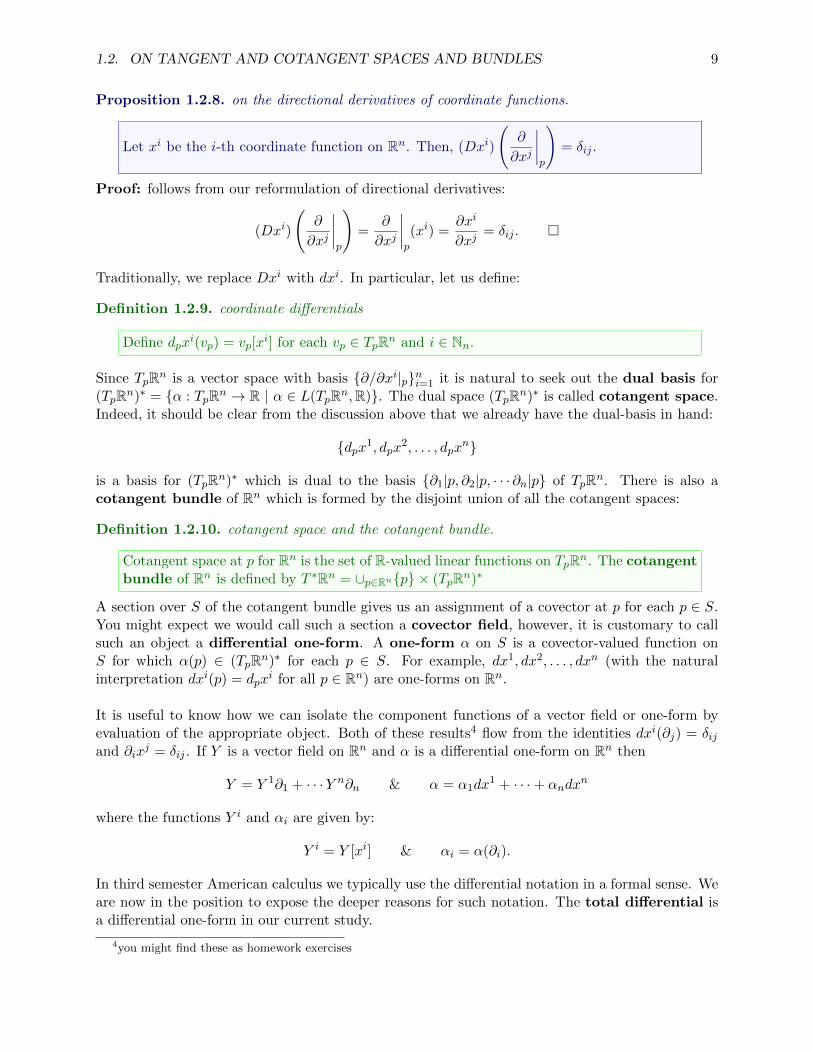
Proposition 1.2.8. on the directional derivatives of coordinate functions.
Let xi be the i-th coordinate function on Rn. Then, (Dxi)
(∂
∂xj
∣∣∣∣p
)= δij .
Proof: follows from our reformulation of directional derivatives:
(Dxi)
(∂
∂xj
∣∣∣∣p
)=
∂
∂xj
∣∣∣∣p
(xi) =∂xi
∂xj= δij . �
Traditionally, we replace Dxi with dxi. In particular, let us define:
Definition 1.2.9. coordinate differentials
Define dpxi(vp) = vp[x
i] for each vp ∈ TpRn and i ∈ Nn.
Since TpRn is a vector space with basis {∂/∂xi|p}ni=1 it is natural to seek out the dual basis for(TpRn)∗ = {α : TpRn → R | α ∈ L(TpRn,R)}. The dual space (TpRn)∗ is called cotangent space.Indeed, it should be clear from the discussion above that we already have the dual-basis in hand:
{dpx1, dpx2, . . . , dpx
n}
is a basis for (TpRn)∗ which is dual to the basis {∂1|p, ∂2|p, · · · ∂n|p} of TpRn. There is also acotangent bundle of Rn which is formed by the disjoint union of all the cotangent spaces:
Definition 1.2.10. cotangent space and the cotangent bundle.
Cotangent space at p for Rn is the set of R-valued linear functions on TpRn. The cotangentbundle of Rn is defined by T ∗Rn = ∪p∈Rn{p} × (TpRn)∗
A section over S of the cotangent bundle gives us an assignment of a covector at p for each p ∈ S.You might expect we would call such a section a covector field, however, it is customary to callsuch an object a differential one-form. A one-form α on S is a covector-valued function onS for which α(p) ∈ (TpRn)∗ for each p ∈ S. For example, dx1, dx2, . . . , dxn (with the naturalinterpretation dxi(p) = dpx
i for all p ∈ Rn) are one-forms on Rn.
It is useful to know how we can isolate the component functions of a vector field or one-form byevaluation of the appropriate object. Both of these results4 flow from the identities dxi(∂j) = δijand ∂ix
j = δij . If Y is a vector field on Rn and α is a differential one-form on Rn then
Y = Y 1∂1 + · · ·Y n∂n & α = α1dx1 + · · ·+ αndx
n
where the functions Y i and αi are given by:
Y i = Y [xi] & αi = α(∂i).
In third semester American calculus we typically use the differential notation in a formal sense. Weare now in the position to expose the deeper reasons for such notation. The total differential isa differential one-form in our current study.
4you might find these as homework exercises

10 CHAPTER 1. INTRODUCTION
Definition 1.2.11. the differential of a real-valued function on Rn
Suppose f : dom(f) ⊆ Rn → R is a smooth function and p ∈ dom(f). The differential off at p is denoted dpf . We define dpf ∈ (TpRn)∗ by
dpf(Y ) = Y [f ]
for each Y ∈ TpRn. The assignment p 7→ dpf gives the differential one-form df on Rn.
Of course, df(∂/∂xi) = ∂f∂xi
hence we find that
df =∂f
∂x1dx1 +
∂f
∂x2dx2 + · · ·+ ∂f
∂xndxn.
Thus, for X ∈ TpRn we arrive at the following formula for the directional derivative of f at p inthe X direction:
(Df)(X)(p) = dpf(X) = X[f ]. (1.1)
If we had a vector field X then df(X) is a function. Likewise, an arbitrary one-form α and a vectorfield X can be combined to form a function α(X).
The following properties of the differential are not difficult to prove:
Proposition 1.2.12. on the directional derivatives of coordinate functions.
Suppose f, g are functions from Rn to R and h is a function on R then
(i.) d(fg) = (df)g + f(dg),
(ii.) d(f + g) = df + dg,
(iii.) d(cf) = cdf ,
(iv.) d(h ◦ f) = h′(f)df .
Proof: I leave the first three to the reader. We prove (iv.). Consider h : R → R and f : Rn → Rand recall the chain-rule:
∂
∂xi[h(f(x))] = h′(f(x))
∂f
∂xi⇒ d(h ◦ f)(xi) = h′(f(x))
∂f
∂xi.
Thus, d(h ◦ f) =
n∑i=1
h′(f(x))∂f
∂xidxi = h′(f(x))
n∑i=1
∂f
∂xidxi = h′(f(x))df. �
Identity (iv.) frees us from our roots.
Example 1.2.13. Let f =√
(x1)2 + · · ·+ (xn)2 clearly f2 = (x1)2 + · · ·+ (xn)2 and thus d(f2) =2fdf and d(f2) = 2x1dx1 + · · ·+ 2xndxn thus
df =x1dx1 + · · ·+ xndxn√
(x1)2 + · · ·+ (xn)2.

1.3. THE WEDGE PRODUCT AND DIFFERENTIAL FORMS 11
1.3 the wedge product and differential forms
We saw in the last section the directional derivative naturally leads us to define the differential of afunction. In particular, we saw that a function f was converted to a one-form df by the operation d.To continue this story we need to introduce the wedge product. The wedge product generalizesthe cross product of three dimensional vector algebra. Or, perhaps it would be more accurate to say,the wedge product allows us a computational device to implement determinants without explicitlywriting determinants. The combination of the wedge product with total differentiation brings usto the exterior derivative. It is the combination of exterior differentiation and the algebra of thewedge product which makes for many elegant simplifications in what would otherwise require muchmore sophisticated calculations. I will admit, it is probably a bit strange at the beginning, but, ifwe stick with it then we’ll gain skills which allow us to do calculus in one of the most general settings.
I’ll define the wedge product formally by it’s properties5. The wedge takes p-form and ”wedges”it with a q-form to make a (p + q)-form. If we take a sum of terms with k differentials wedgedtogether then this gives us a k-form. A 0-form is a function. A 1-form is an expression of the formα =
∑i αidx
i where αi are functions. A 2-form can be written as β =∑
i,j12βijdx
i ∧ dxj where
βij are functions. A k-form can be written γ =∑
i1,...,ik1k!γi1,...,ikdx
i1 ∧ · · · ∧ dxik where γi1,...,ik arefunctions. The essential properties of the wedge product are as follows:
(i.) ∧ is an associative product; α ∧ (β ∧ γ) = (α ∧ β) ∧ γ.
(ii.) ∧ is anticommutative on differentials; dxi ∧ dxj = −dxj ∧ dxi
(iii.) ∧ has a distributive property; α ∧ (β + γ) = α ∧ β + α ∧ γ.
It’s not much work to show ∧ is anticommutative on arbitary one-forms. If α =∑
i αidxi and
β =∑
j βjdxj are one forms then, by the above properties:
α ∧ β =
(∑i
αidxi
)∧
∑j
βjdxj
=∑i
∑j
αiβjdxi ∧ dxj
= −∑j
∑i
βjαidxj ∧ dxi
= −
∑j
βjdxj
(∑i
αidxi
)= −β ∧ α.
Up to this point I have indicated our differential forms have coefficients which are functions. If wewere to follow terminology similar to that for vectors then we would rather call differential formssomething like form-fields. However, this is not usually done. Naturally, if we wished to work at asingle point then the functions mentioned above would be traded for sets of constants6.
5there are elegant ways in terms of abstract algebra, or the concrete multilinear mapping discussion you can seein my advanced calculus notes, here, I just say how it works
6we could discuss the algebra of wedge products of a given vector space V without any discussion of differentials,but, I mostly keep our focus on the objects we use for the calculational core of this course. The wedge product algebrawould provide another way to capture linear independence. For example, v ∧ w = 0 iff v is linearly dependent on w.The same holds for a k-fold wedge product. In contrast, determinants worked only for n-vectors in Rn.
12 CHAPTER 1. INTRODUCTION
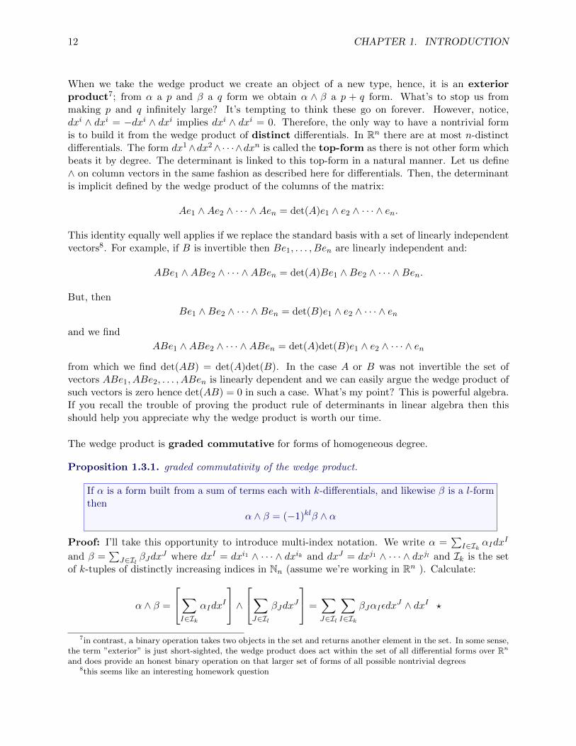
When we take the wedge product we create an object of a new type, hence, it is an exteriorproduct7; from α a p and β a q form we obtain α ∧ β a p + q form. What’s to stop us frommaking p and q infinitely large? It’s tempting to think these go on forever. However, notice,dxi ∧ dxi = −dxi ∧ dxi implies dxi ∧ dxi = 0. Therefore, the only way to have a nontrivial formis to build it from the wedge product of distinct differentials. In Rn there are at most n-distinctdifferentials. The form dx1∧dx2∧· · ·∧dxn is called the top-form as there is not other form whichbeats it by degree. The determinant is linked to this top-form in a natural manner. Let us define∧ on column vectors in the same fashion as described here for differentials. Then, the determinantis implicit defined by the wedge product of the columns of the matrix:
Ae1 ∧Ae2 ∧ · · · ∧Aen = det(A)e1 ∧ e2 ∧ · · · ∧ en.
This identity equally well applies if we replace the standard basis with a set of linearly independentvectors8. For example, if B is invertible then Be1, . . . , Ben are linearly independent and:
ABe1 ∧ABe2 ∧ · · · ∧ABen = det(A)Be1 ∧Be2 ∧ · · · ∧Ben.
But, then
Be1 ∧Be2 ∧ · · · ∧Ben = det(B)e1 ∧ e2 ∧ · · · ∧ en
and we find
ABe1 ∧ABe2 ∧ · · · ∧ABen = det(A)det(B)e1 ∧ e2 ∧ · · · ∧ en
from which we find det(AB) = det(A)det(B). In the case A or B was not invertible the set ofvectors ABe1, ABe2, . . . , ABen is linearly dependent and we can easily argue the wedge product ofsuch vectors is zero hence det(AB) = 0 in such a case. What’s my point? This is powerful algebra.If you recall the trouble of proving the product rule of determinants in linear algebra then thisshould help you appreciate why the wedge product is worth our time.
The wedge product is graded commutative for forms of homogeneous degree.
Proposition 1.3.1. graded commutativity of the wedge product.
If α is a form built from a sum of terms each with k-differentials, and likewise β is a l-formthen
α ∧ β = (−1)klβ ∧ α
Proof: I’ll take this opportunity to introduce multi-index notation. We write α =∑
I∈Ik αIdxI
and β =∑
J∈Il βJdxJ where dxI = dxi1 ∧ · · · ∧ dxik and dxJ = dxj1 ∧ · · · ∧ dxjl and Ik is the set
of k-tuples of distinctly increasing indices in Nn (assume we’re working in Rn ). Calculate:
α ∧ β =
∑I∈Ik
αIdxI
∧∑J∈Il
βJdxJ
=∑J∈Il
∑I∈Ik
βJαIεdxJ ∧ dxI ?
7in contrast, a binary operation takes two objects in the set and returns another element in the set. In some sense,the term ”exterior” is just short-sighted, the wedge product does act within the set of all differential forms over Rnand does provide an honest binary operation on that larger set of forms of all possible nontrivial degrees
8this seems like an interesting homework question
1.3. THE WEDGE PRODUCT AND DIFFERENTIAL FORMS 13
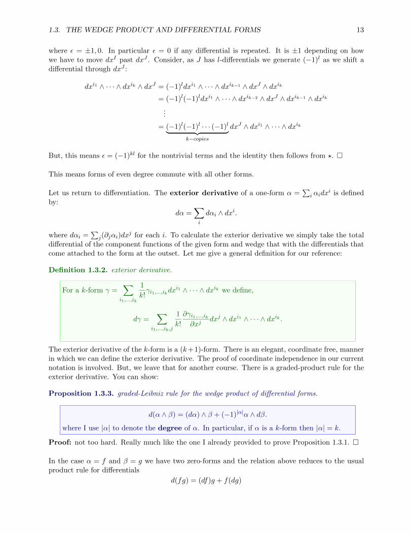
where ε = ±1, 0. In particular ε = 0 if any differential is repeated. It is ±1 depending on howwe have to move dxI past dxJ . Consider, as J has l-differentials we generate (−1)l as we shift adifferential through dxJ :
dxi1 ∧ · · · ∧ dxik ∧ dxJ = (−1)ldxi1 ∧ · · · ∧ dxik−1 ∧ dxJ ∧ dxik
= (−1)l(−1)ldxi1 ∧ · · · ∧ dxik−2 ∧ dxJ ∧ dxik−1 ∧ dxik...
= (−1)l(−1)l · · · (−1)l︸ ︷︷ ︸k−copies
dxJ ∧ dxi1 ∧ · · · ∧ dxik
But, this means ε = (−1)kl for the nontrivial terms and the identity then follows from ?. �
This means forms of even degree commute with all other forms.
Let us return to differentiation. The exterior derivative of a one-form α =∑
i αidxi is defined
by:
dα =∑i
dαi ∧ dxi.
where dαi =∑
j(∂jαi)dxj for each i. To calculate the exterior derivative we simply take the total
differential of the component functions of the given form and wedge that with the differentials thatcome attached to the form at the outset. Let me give a general definition for our reference:
Definition 1.3.2. exterior derivative.
For a k-form γ =∑i1,...,ik
1
k!γi1,...,ikdx
i1 ∧ · · · ∧ dxik we define,
dγ =∑
i1,...,ik,j
1
k!
∂γi1,...,ik∂xj
dxj ∧ dxi1 ∧ · · · ∧ dxik .
The exterior derivative of the k-form is a (k+1)-form. There is an elegant, coordinate free, mannerin which we can define the exterior derivative. The proof of coordinate independence in our currentnotation is involved. But, we leave that for another course. There is a graded-product rule for theexterior derivative. You can show:
Proposition 1.3.3. graded-Leibniz rule for the wedge product of differential forms.
d(α ∧ β) = (dα) ∧ β + (−1)|α|α ∧ dβ.
where I use |α| to denote the degree of α. In particular, if α is a k-form then |α| = k.
Proof: not too hard. Really much like the one I already provided to prove Proposition 1.3.1. �
In the case α = f and β = g we have two zero-forms and the relation above reduces to the usualproduct rule for differentials
d(fg) = (df)g + f(dg)
14 CHAPTER 1. INTRODUCTION
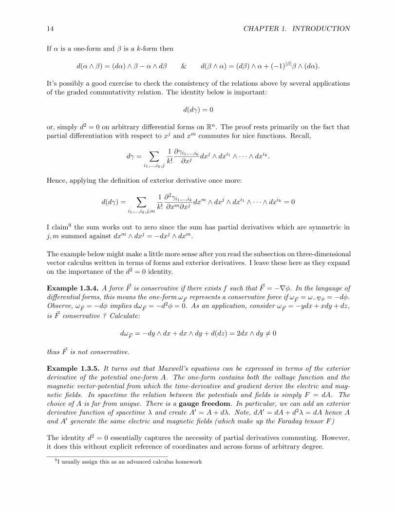
If α is a one-form and β is a k-form then
d(α ∧ β) = (dα) ∧ β − α ∧ dβ & d(β ∧ α) = (dβ) ∧ α+ (−1)|β|β ∧ (dα).
It’s possibly a good exercise to check the consistency of the relations above by several applicationsof the graded commutativity relation. The identity below is important:
d(dγ) = 0
or, simply d2 = 0 on arbitrary differential forms on Rn. The proof rests primarily on the fact thatpartial differentiation with respect to xj and xm commutes for nice functions. Recall,
dγ =∑
i1,...,ik,j
1
k!
∂γi1,...,ik∂xj
dxj ∧ dxi1 ∧ · · · ∧ dxik .
Hence, applying the definition of exterior derivative once more:
d(dγ) =∑
i1,...,ik,j,m
1
k!
∂2γi1,...,ik∂xm∂xj
dxm ∧ dxj ∧ dxi1 ∧ · · · ∧ dxik = 0
I claim9 the sum works out to zero since the sum has partial derivatives which are symmetric inj,m summed against dxm ∧ dxj = −dxj ∧ dxm.
The example below might make a little more sense after you read the subsection on three-dimensionalvector calculus written in terms of forms and exterior derivatives. I leave these here as they expandon the importance of the d2 = 0 identity.
Example 1.3.4. A force ~F is conservative if there exists f such that ~F = −∇φ. In the langauge ofdifferential forms, this means the one-form ω~F represents a conservative force if ω~F = ω−∇φ = −dφ.Observe, ω~F = −dφ implies dω~F = −d2φ = 0. As an application, consider ω~F = −ydx+ xdy+ dz,
is ~F conservative ? Calculate:
dω~F = −dy ∧ dx+ dx ∧ dy + d(dz) = 2dx ∧ dy 6= 0
thus ~F is not conservative.
Example 1.3.5. It turns out that Maxwell’s equations can be expressed in terms of the exteriorderivative of the potential one-form A. The one-form contains both the voltage function and themagnetic vector-potential from which the time-derivative and gradient derive the electric and mag-netic fields. In spacetime the relation between the potentials and fields is simply F = dA. Thechoice of A is far from unique. There is a gauge freedom. In particular, we can add an exteriorderivative function of spacetime λ and create A′ = A + dλ. Note, dA′ = dA + d2λ = dA hence Aand A′ generate the same electric and magnetic fields (which make up the Faraday tensor F )
The identity d2 = 0 essentially captures the necessity of partial derivatives commuting. However,it does this without explicit reference of coordinates and across forms of arbitrary degree.
9I usually assign this as an advanced calculus homework
1.3. THE WEDGE PRODUCT AND DIFFERENTIAL FORMS 15
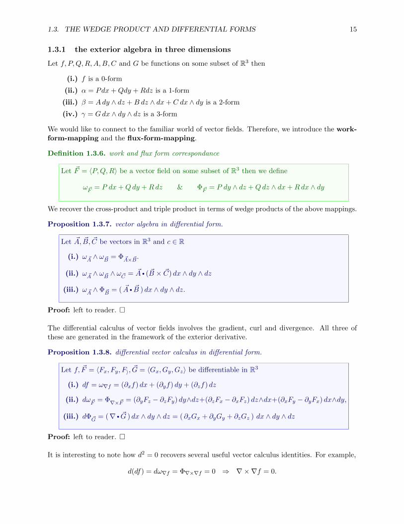
1.3.1 the exterior algebra in three dimensions
Let f, P,Q,R,A,B,C and G be functions on some subset of R3 then
(i.) f is a 0-form
(ii.) α = Pdx+Qdy +Rdz is a 1-form
(iii.) β = Ady ∧ dz +B dz ∧ dx+ C dx ∧ dy is a 2-form
(iv.) γ = Gdx ∧ dy ∧ dz is a 3-form
We would like to connect to the familiar world of vector fields. Therefore, we introduce the work-form-mapping and the flux-form-mapping.
Definition 1.3.6. work and flux form correspondance
Let ~F = 〈P,Q,R〉 be a vector field on some subset of R3 then we define
ω~F = P dx+Qdy +Rdz & Φ~F = P dy ∧ dz +Qdz ∧ dx+Rdx ∧ dy
We recover the cross-product and triple product in terms of wedge products of the above mappings.
Proposition 1.3.7. vector algebra in differential form.
Let ~A, ~B, ~C be vectors in R3 and c ∈ R
(i.) ω ~A ∧ ω ~B = Φ ~A× ~B.
(ii.) ω ~A ∧ ω ~B ∧ ω ~C = ~A • ( ~B × ~C) dx ∧ dy ∧ dz
(iii.) ω ~A ∧ Φ ~B = ( ~A • ~B ) dx ∧ dy ∧ dz.
Proof: left to reader. �
The differential calculus of vector fields involves the gradient, curl and divergence. All three ofthese are generated in the framework of the exterior derivative.
Proposition 1.3.8. differential vector calculus in differential form.
Let f, ~F = 〈Fx, Fy, F〉, ~G = 〈Gx, Gy, Gz〉 be differentiable in R3
(i.) df = ω∇f = (∂xf) dx+ (∂yf) dy + (∂zf) dz
(ii.) dω~F = Φ∇×~F = (∂yFz − ∂zFy) dy∧dz+(∂zFx − ∂xFz) dz∧dx+(∂xFy − ∂yFx) dx∧dy,
(iii.) dΦ ~G = (∇ • ~G ) dx ∧ dy ∧ dz = ( ∂xGx + ∂yGy + ∂zGz ) dx ∧ dy ∧ dz
Proof: left to reader. �
It is interesting to note how d2 = 0 recovers several useful vector calculus identities. For example,
d(df) = dω∇f = Φ∇×∇f = 0 ⇒ ∇×∇f = 0.
16 CHAPTER 1. INTRODUCTION
or,
d(dω~F ) = dΦ∇×~F = ∇ • (∇× ~F ) dx ∧ dy ∧ dz = 0 ⇒ ∇ • (∇× ~F ) = 0.
The graded Leibniz rule also reveals several interesting product rules. For example,
d(ω ~A ∧ ω ~B) = dω ~A ∧ ω ~B − ω ~A ∧ dω ~B= Φ∇× ~A ∧ ω ~B − ω ~A ∧ Φ∇× ~B
=(
(∇× ~A) • ~B − ~A • (∇× ~B))dx ∧ dy ∧ dz.
But, we also know ω ~A ∧ ω ~B = Φ ~A× ~B hence
d(ω ~A ∧ ω ~B) = dΦ ~A× ~B = ∇ • ( ~A× ~B) dx ∧ dy ∧ dz.
Therefore, ∇ • ( ~A× ~B) = (∇× ~A) • ~B− ~A • (∇× ~B). I can derive this with Levi-Civita calculationswithout much trouble, but, I wonder, can you ? The point I intend to make here: the wedge productautomatically builds all manner of complicated vector identities into a few simple, generalizable,algebraic operations. The beauty of differential forms in revealing the true structure of integralvector calculus is no less shocking. But, I leave it for another time. In fact, I leave many thingsfor another time here. I merely hope we’ve said enough to make our use of the wedge product andexterior calculus a bit less bizarre in the remainder of the course.
1.4 paths and curves
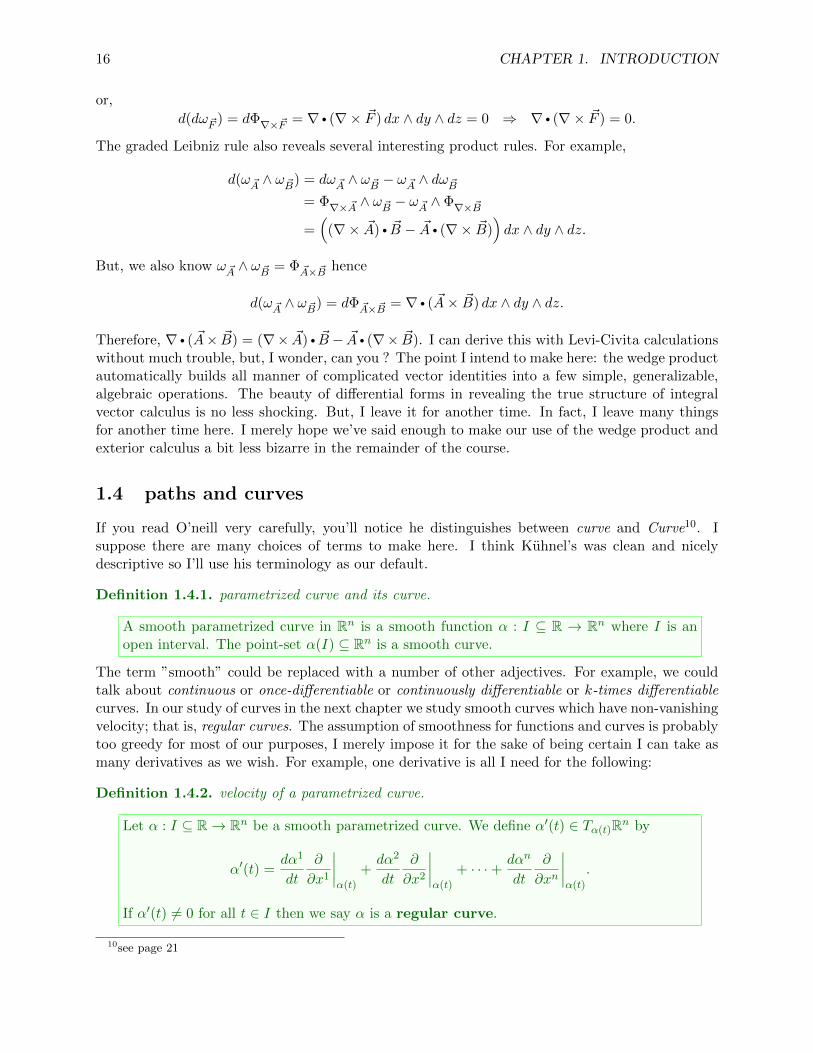
If you read O’neill very carefully, you’ll notice he distinguishes between curve and Curve10. Isuppose there are many choices of terms to make here. I think Kuhnel’s was clean and nicelydescriptive so I’ll use his terminology as our default.
Definition 1.4.1. parametrized curve and its curve.
A smooth parametrized curve in Rn is a smooth function α : I ⊆ R → Rn where I is anopen interval. The point-set α(I) ⊆ Rn is a smooth curve.
The term ”smooth” could be replaced with a number of other adjectives. For example, we couldtalk about continuous or once-differentiable or continuously differentiable or k-times differentiablecurves. In our study of curves in the next chapter we study smooth curves which have non-vanishingvelocity; that is, regular curves. The assumption of smoothness for functions and curves is probablytoo greedy for most of our purposes, I merely impose it for the sake of being certain I can take asmany derivatives as we wish. For example, one derivative is all I need for the following:
Definition 1.4.2. velocity of a parametrized curve.
Let α : I ⊆ R→ Rn be a smooth parametrized curve. We define α′(t) ∈ Tα(t)Rn by
α′(t) =dα1
dt
∂
∂x1
∣∣∣∣α(t)
+dα2
dt
∂
∂x2
∣∣∣∣α(t)
+ · · ·+ dαn
dt
∂
∂xn
∣∣∣∣α(t)
.
If α′(t) 6= 0 for all t ∈ I then we say α is a regular curve.
10see page 21

1.4. PATHS AND CURVES 17
On pages 7-8 of Kuhnel discusses why regularity is a good requirement for us to make for the curveswe wish to study. Of course, we could use less structure, but then we’d face pathological examplessuch as parametrized curves whose curve fill a rectangle in the plane, or differentiable curves whichhave infinitely many corners. The criteria of regularity keeps these odd features outside our study.From a big-picture perspective, regularity is a full-rank condition since the highest dimension pos-sible for the tangent space to a curve is one and regularity demands the rank of the tangent spacebe everywhere maximal on the curve. We soon discuss similar conditions for mappings in the finalsection of this chapter.
The velocity of a parametrized curve is an operator on functions defined near the curve. Consider:
α′(t)[f ] =
(dα1
dt
∂
∂x1
∣∣∣∣α(t)
+dα2
dt
∂
∂x2
∣∣∣∣α(t)
+ · · ·+ dαn
dt
∂
∂xn
∣∣∣∣α(t)
)[f ]
=dα1
dt
∂f
∂x1(α(t)) +
dα2
dt
∂f
∂x2(α(t)) + · · ·+ dαn
dt
∂f
∂xn(α(t))
=d
dt[f(α(t))]
where in the last step we used the chain-rule for f ◦α. The velocity α′(t) acts on f to tell us howf changes along α at α(t). We record this result for future reference:
Proposition 1.4.3. change of function along curve.
Suppose α is a parametrized curve and f is a smooth function defined near α(t) for some
t ∈ dom(α) then α′(t)[f ] =d(f ◦α)
dt.
Example 1.4.4. Let α(t) = p + t(q − p) for a given pair of distinct points p, q ∈ Rn. You shouldidentify α as the line connecting point p = α(0) and q = α(1). If we define v = q − p then thevelocity of α is given by:
α′(t) = v1 ∂
∂x1
∣∣∣∣α(t)
+ v2 ∂
∂x2
∣∣∣∣α(t)
+ · · ·+ vn∂
∂xn
∣∣∣∣α(t)
Specializing to n = 2 and v = 〈a, b〉 we have α(t) = (p1 + ta, p2 + tb) and
α′(t) = a∂
∂x
∣∣∣∣α(t)
+ b∂
∂y
∣∣∣∣α(t)
Let f(x, y) = x2 + y2 then
α′(t)[f ] =
(a∂
∂x
∣∣∣∣α(t)
+ b∂
∂y
∣∣∣∣α(t)
)[x2 + y2] = (2xa+ 2yb)
∣∣α(t)
= 2(p1 + ta)a+ 2(p2 + tb)b.
As an easy to check case, take p = (0, 0) hence p1 = 0 and p2 = 0 hence α′(t)[f ] = 2t(a2 + b2). Fort > 0 we see f is increasing as we travel away from the origin along the line α(t). But, f is justthe distance from the origin squared so the rate of change is quite reasonable. If we were to imposea2 + b2 = 1 then t represents the distance from the origin and the result reduces to α′(t)[f ] = 2twhich makes sense as f(α(t)) = (ta)2 + (tb)2 = t2(a2 + b2) = t2.

18 CHAPTER 1. INTRODUCTION
Notice that α′(t)[f ] gives the usual third-semester-American calculus directional derivative in thedirection of α′(t) only if we choose a parameter t for which ||α′(t)|| = 1. This choice of parametriza-tion is known as the arclength or unit-speed parametrization.
Example 1.4.5. Let R,m > 0 be constants and α(t) = (R cos t, R sin t,mt) for t ∈ R. We say αis a helix with slope m and radius R. Notice α(t) falls on the cylinder x2 + y2 = R2. Of course,we could define helices around other circular cylinders. The velocity vector field for α is given by:
α′(t) =
(−R sin t
∂
∂x+R cos t
∂
∂y+m
∂
∂z
) ∣∣∣∣α(t)
Then, f(x, y, z) = x2 + y2 has
α′(t)[f ] = (−2xR sin t+ 2yR cos t)|α(t) = −2R2 cos t sin t+ 2R2 sin t cos t = 0.
This is in good agreement with Proposition 1.4.3 as f(α(t)) = R2 is constant. On the other hand,g(x, y, z) = z gives α′(t)[g] = m which shows m is proportional to the rate at which the helix risesin z. To obtain the absolute rate we would need to derive the arclength-parametrization of α.
A given curve has infinitely many parametrizations.
Definition 1.4.6. reparametrization of curve.
Let α : I ⊆ R → Rn be a parametrized curve. If h : J → I is a smooth function onan open interval J then β = α ◦h : J → Rn is a parametrized curve which we call thereparametrization of α by h.
The definition above is a bit more general than I usually give in third-semester American calculusin the sense that the reparametrization need not cover the same curve. It could be that the curveof the reparametrization is just a subset of the curve of the original parametrized curve. Also, wedid not assume h is injective which means β might not share the same orientation as α.
Proposition 1.4.7. velocity of reparametrized curve
If α is a parametrized curve β = α ◦h is a reparametrization of α by h then
β′(s) =dh
dsα′(h(s))
Proof: by definition,
β′(s) =dβ1
ds
∂
∂x1
∣∣∣∣β(s)
+dβ2
ds
∂
∂x2
∣∣∣∣β(s)
+ · · ·+ dβn
ds
∂
∂xn
∣∣∣∣β(s)
But, β(s) = α(h(s)) hence dβj
ds = ddsα
j(h(s)) = dαj
ds (h(s))dhds for each j and we find a factor of dhds on
each term which when factored out yields:
β′(s) =dh
ds
[d(α ◦h)1
ds
∂
∂x1
∣∣∣∣α(h(s))
+d(α ◦h)2
ds
∂
∂x1
∣∣∣∣α(h(s))
+ · · ·+ d(α ◦h)1
ds
∂
∂xn
∣∣∣∣α(h(s))
]the proposition follows immediately as the term in square-brackets is precisely α′(h(s)). �
Honestly, the theorem above is not new. We also had this theorem in multivariate calculus. Thenew thing is merely the notation for expressing vectors attached to a point as derivations. I includethe proof here merely to show how we work with such notation.
1.5. THE PUSH-FORWARD OR DIFFERENTIAL OF A MAP 19
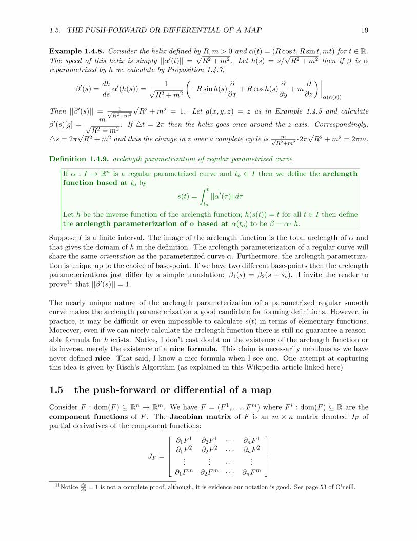
Example 1.4.8. Consider the helix defined by R,m > 0 and α(t) = (R cos t, R sin t,mt) for t ∈ R.The speed of this helix is simply ||α′(t)|| =
√R2 +m2. Let h(s) = s/
√R2 +m2 then if β is α
reparametrized by h we calculate by Proposition 1.4.7,
β′(s) =dh
dsα′(h(s)) =
1√R2 +m2
(−R sinh(s)
∂
∂x+R cosh(s)
∂
∂y+m
∂
∂z
) ∣∣∣∣α(h(s))
Then ||β′(s)|| = 1√R2+m2
√R2 +m2 = 1. Let g(x, y, z) = z as in Example 1.4.5 and calculate
β′(s)[g] =m√
R2 +m2. If 4t = 2π then the helix goes once around the z-axis. Correspondingly,
4s = 2π√R2 +m2 and thus the change in z over a complete cycle is m√
R2+m2·2π√R2 +m2 = 2πm.
Definition 1.4.9. arclength parametrization of regular parametrized curve
If α : I → Rn is a regular parametrized curve and to ∈ I then we define the arclengthfunction based at to by
s(t) =
∫ t
to
||α′(τ)||dτ
Let h be the inverse function of the arclength function; h(s(t)) = t for all t ∈ I then definethe arclength parameterization of α based at α(to) to be β = α ◦h.
Suppose I is a finite interval. The image of the arclength function is the total arclength of α andthat gives the domain of h in the definition. The arclength parameterization of a regular curve willshare the same orientation as the parameterized curve α. Furthermore, the arclength parametriza-tion is unique up to the choice of base-point. If we have two different base-points then the arclengthparameterizations just differ by a simple translation: β1(s) = β2(s + so). I invite the reader toprove11 that ||β′(s)|| = 1.
The nearly unique nature of the arclength parameterization of a parametrized regular smoothcurve makes the arclength parameterization a good candidate for forming definitions. However, inpractice, it may be difficult or even impossible to calculate s(t) in terms of elementary functions.Moreover, even if we can nicely calculate the arclength function there is still no guarantee a reason-able formula for h exists. Notice, I don’t cast doubt on the existence of the arclength function orits inverse, merely the existence of a nice formula. This claim is necessarily nebulous as we havenever defined nice. That said, I know a nice formula when I see one. One attempt at capturingthis idea is given by Risch’s Algorithm (as explained in this Wikipedia article linked here)
1.5 the push-forward or differential of a map
Consider F : dom(F ) ⊆ Rn → Rm. We have F = (F 1, . . . , Fm) where F i : dom(F ) ⊆ R are thecomponent functions of F . The Jacobian matrix of F is an m × n matrix denoted JF ofpartial derivatives of the component functions:
JF =
∂1F
1 ∂2F1 · · · ∂nF
1
∂1F2 ∂2F
2 · · · ∂nF2
...... · · ·
...∂1F
m ∂2Fm · · · ∂nF
m
11Notice ds
ds= 1 is not a complete proof, although, it is evidence our notation is good. See page 53 of O’neill.
20 CHAPTER 1. INTRODUCTION
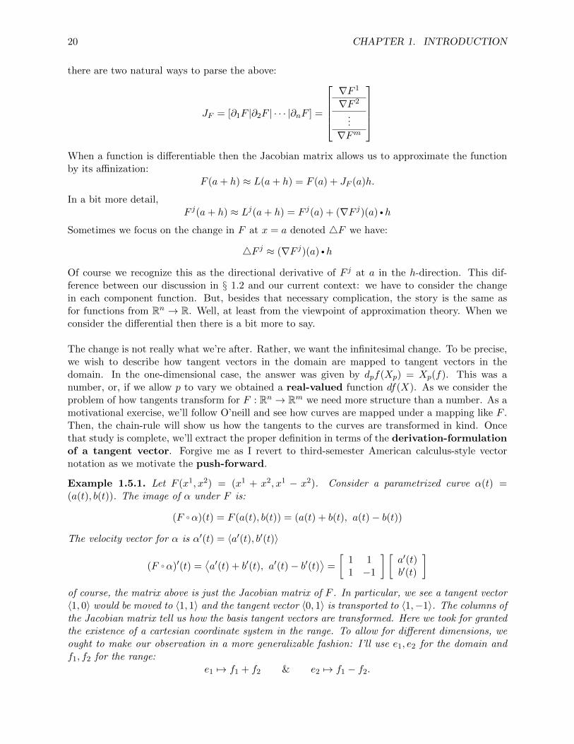
there are two natural ways to parse the above:
JF = [∂1F |∂2F | · · · |∂nF ] =
∇F 1
∇F 2
...
∇Fm
When a function is differentiable then the Jacobian matrix allows us to approximate the functionby its affinization:
F (a+ h) ≈ L(a+ h) = F (a) + JF (a)h.
In a bit more detail,F j(a+ h) ≈ Lj(a+ h) = F j(a) + (∇F j)(a) •h
Sometimes we focus on the change in F at x = a denoted 4F we have:
4F j ≈ (∇F j)(a) •h
Of course we recognize this as the directional derivative of F j at a in the h-direction. This dif-ference between our discussion in § 1.2 and our current context: we have to consider the changein each component function. But, besides that necessary complication, the story is the same asfor functions from Rn → R. Well, at least from the viewpoint of approximation theory. When weconsider the differential then there is a bit more to say.
The change is not really what we’re after. Rather, we want the infinitesimal change. To be precise,we wish to describe how tangent vectors in the domain are mapped to tangent vectors in thedomain. In the one-dimensional case, the answer was given by dpf(Xp) = Xp(f). This was anumber, or, if we allow p to vary we obtained a real-valued function df(X). As we consider theproblem of how tangents transform for F : Rn → Rm we need more structure than a number. As amotivational exercise, we’ll follow O’neill and see how curves are mapped under a mapping like F .Then, the chain-rule will show us how the tangents to the curves are transformed in kind. Oncethat study is complete, we’ll extract the proper definition in terms of the derivation-formulationof a tangent vector. Forgive me as I revert to third-semester American calculus-style vectornotation as we motivate the push-forward.
Example 1.5.1. Let F (x1, x2) = (x1 + x2, x1 − x2). Consider a parametrized curve α(t) =(a(t), b(t)). The image of α under F is:
(F ◦α)(t) = F (a(t), b(t)) = (a(t) + b(t), a(t)− b(t))
The velocity vector for α is α′(t) = 〈a′(t), b′(t)〉
(F ◦α)′(t) =⟨a′(t) + b′(t), a′(t)− b′(t)
⟩=
[1 11 −1
] [a′(t)b′(t)
]of course, the matrix above is just the Jacobian matrix of F . In particular, we see a tangent vector〈1, 0〉 would be moved to 〈1, 1〉 and the tangent vector 〈0, 1〉 is transported to 〈1,−1〉. The columns ofthe Jacobian matrix tell us how the basis tangent vectors are transformed. Here we took for grantedthe existence of a cartesian coordinate system in the range. To allow for different dimensions, weought to make our observation in a more generalizable fashion: I’ll use e1, e2 for the domain andf1, f2 for the range:
e1 7→ f1 + f2 & e2 7→ f1 − f2.

1.5. THE PUSH-FORWARD OR DIFFERENTIAL OF A MAP 21
Now, in the derivation notation for tangent vectors, e1 = ∂∂x1
, e2 = ∂∂x2
and for cartesian coordinates
(y1, y2) for the range f1 = ∂∂y1
, f2 = ∂∂y2
. We have:
∂
∂x17→ ∂
∂y1+
∂
∂y2&
∂
∂x27→ ∂
∂y1− ∂
∂y2.
Example 1.5.2. Another example, F (x1, x2) = (ex1+x2 , sinx2, cosx2). Once more, consider the
curve α = (a, b) hence α′ = 〈a′, b′〉 and
(F ◦α)′ = 〈ea+b(a′ + b′), (cos b)b′, (− sin b)b′〉
We find the tangent 〈a′, b′〉 = 〈1, 0〉 maps to 〈ea+b, 0, 0〉 whereas the tangent 〈a′, b′〉 = 〈0, 1〉 mapsto 〈ea+b, cos b, − sin b〉 with respect to the point α = (a, b) of the curve. The Jacobian of F at (a, b)is:
JF (a, b) =
ea+b ea+b
0 cos b0 − sin b
.Following the notation of the last example, but now with (y1, y2, y3) coordinates for the image,
∂
∂x17→ ea+b ∂
∂y1&
∂
∂x27→ ea+b ∂
∂y1+ cos b
∂
∂y2− sin b
∂
∂y3.
Notice, yj ◦F = F j is immediate from the definition of cartesian coordinates and component func-tions. What we really have above is:
∂
∂x17→
3∑j=1
∂(yj ◦F )
∂x1
∂
∂yj&
∂
∂x27→
3∑j=1
∂(yj ◦F )
∂x2
∂
∂yj
But, even the above is not quite accurate as it does not indicate the true point-dependence. Annoy-ingly, I must write:
∂
∂x1
∣∣∣∣p
7→3∑j=1
∂(yj ◦F )
∂x1(p)
∂
∂yj
∣∣∣∣F (p)
&∂
∂x2
∣∣∣∣p
7→3∑j=1
∂(yj ◦F )
∂x2(p)
∂
∂yj
∣∣∣∣F (p)
Of course, including the point-dependence on the cartesian coordinate derivations in overkill. How-ever, later when we deal with curved coordinate systems the coordinate derivations will aquire apoint-dependence like r or θ (discussed in my multivariate callculus notes).
From § 1.2 recall that we may write∂F j
∂xi(p) = dpF
j
(∂
∂xi∣∣p
). Thus, recognizing F j = yj ◦F we
find the result of our last motivating example can be written:
∂
∂xi∣∣p7→
3∑j=1
dpFj
(∂
∂xi∣∣p
)∂
∂yj
∣∣∣∣F (p)
.
Extending this linearly brings us to see why the next definition is made:

22 CHAPTER 1. INTRODUCTION
Definition 1.5.3. differential of a mapping or, the push-forward
Let F : Rn → Rm be a differentiable function at p and suppose X ∈ TpRn and y1, . . . , ym areCartesian coordinates such that F j = yj ◦F for each j ∈ Nm then we define the differentialof F at p to be the mapping from TpRn to TF (p)Rm defined by:
dpF (X) =
m∑j=1
dpFj (X)
∂
∂yj
∣∣∣∣F (p)
.
Alternatively, we may denote dpF (X) = F∗p(X). Or, is we wish to think of p as varyingthen p 7→ dpF may be denoted F∗ or dF .
It is also useful to view the above in slightly different terms:
dpF (X) =m∑j=1
X[F j ]∂
∂yj
∣∣∣∣F (p)
.
If we permit the identification of the formula of F with the coordinates in the image, that is we setF j = yj then the formula simplifies further:
dpF
(∂
∂xi
∣∣∣∣p
)=
m∑j=1
∂yj
∂xi∂
∂yj
∣∣∣∣F (p)
.
Perhaps you saw such a calculation in your multivariate calculus course. For example, the problemof writing ∂/∂r in terms of derivatives with respect to x, y.
∂
∂r=∂x
∂r
∂
∂x+∂y
∂r
∂
∂y= cos θ
∂
∂x+ sin θ
∂
∂y.
This is the push-forward of ∂/∂r with respect to the map F (r, θ) = (r cos θ, r sin θ) where the do-main and range of F are viewed as the same plane. Thus, we observe the push-forward is sometimesunderstood as a coordinate change. However, this is a special case as generally the domain andcodomain need not be the same set, or even the same dimension.
The reason F∗ is called the push-forward is that it pushes a vector field in the domain of F toanother vector field in the range of F . Well, not so fast, the previous sentence is only true if Fdoes not misbehave. For example, if F thrice wraps a circle in the domain around an oval in theimage then we might have several vectors mapped to a given point on the oval. A vector field is anassignment of one vector to each point, so, F∗(X) would not be a vector field in such a case. Onthe other hand, if F is injective locally then we can expect to map vector fields to vector fields bypush-forward of the restriction of F .
In the advanced calculus course we show that local injectivity for a continuously differentiablefunction F : Rn → Rm is implied by the injectivity of the differential of the function at a point. Inparticular, we define F to be regular at p if the differential dpF is full-rank. If F : Rn → Rm thendpF has full-rank at p if JF (p) has n-linearly-independent columns. The inverse function theo-rem states that when F is a continuously differentiable function which is regular at p then thereexist U ⊆ Rn and V ⊆ Rm for which F |U : U → V is invertible with continuously differentiableinverse. In the case n = m we can check the regularity of F at p by showin detJF (p) 6= 0. This the-orem is a local result in the sense that it does not imply the invertibilty of F for its whole domain.

1.5. THE PUSH-FORWARD OR DIFFERENTIAL OF A MAP 23
For example, the polar coordinate transformation is locally invertible away from the origin, but,it always faces the 2π-angle degeneracy if we have a domain which includes a circle around the origin.
The other theorem we need at times from advanced calculus is the implicit function theorem.If F : Rr ×Rn → Rn is continuously differentiable with n-linearly-independent final columns in JFat (q, p) then we can find a continuously differentiable function G : Rn → Rr such that q = G(p)and y = G(x) solves F (x, y) = c for (x, y) near (q, p). I think this is a bit harder to understand.Let me just give two examples which illustrate a typical use of the theorem to express curves andsurfaces as graphs.
Example 1.5.4. Let F (x, y) = x2 + y2 then F (x, y) = R2 is a circle and
JF =[
2x 2y]
we see y 6= 0 implies the last column is nonzero hence we may solve for y near such points. In thiscase, G(x) = ±
√R2 − x2 where we choose ± appropriate to the location of the local solution.
Example 1.5.5. Let F (x, y, z) = cos(x) + y + z2 then
JF =[− sin(x) 1 2z
]this tells me I can solve for z = z(x, y) when z 6= 0, or I can solve for y = y(x, z) anywhere onF (x, y, z) = c, or I can solve for x = x(y, z) when x 6= nπ for n ∈ Z. Notice we can rearrangecoordinates to put x or y as the last coordinate.
I conclude this section with a few comments which ought to be made somewhere. You can skipthem in the first reading of these notes.
The definition I offer above is actually not the definition given in O’neill. Rather, O’neill definesF∗p as the mapping which takes tangents at p with velocity v to tangents of F (p + tv) at F (p).Then he derives from that the result:
F∗(α′) = β′
where β = F ◦α. In fact, the above result is sometimes used to define the differential. Thisdefinition is elegant and has certain advantages over my coordinate-based definition. The reasonfor the different defnitions is simply that we have freedom to view tangent vectors in differentialgeometry in several formalisms. To be careful, if I was to use the curve definition, I would use anequivalence class of curves and write:
dpF ([α′]) = [(F ◦α)′]
You can define an isomorphism between equivalence classes of curves and derivations of smoothfunctions at a given point. Then, if you translate O’neill’s curve-based definition through thatisomorphism then you’ll obtain the definition I gave in this section. Both formulations have theirmerit and O’neill has a way of using both without being explicit. The explicit nature of what I sayhere ruins the art of the presentation. My apologies.
24 CHAPTER 1. INTRODUCTION
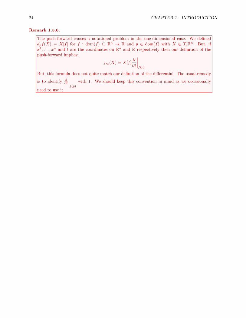
Remark 1.5.6.
The push-forward causes a notational problem in the one-dimensional case. We defineddpf(X) = X[f ] for f : dom(f) ⊆ Rn → R and p ∈ dom(f) with X ∈ TpRn. But, ifx1, . . . , xn and t are the coordinates on Rn and R respectively then our definition of thepush-forward implies:
f∗p(X) = X[f ]∂
∂t
∣∣∣∣f(p)
But, this formula does not quite match our definition of the differential. The usual remedy
is to identify ∂∂t
∣∣∣∣f(p)
with 1. We should keep this convention in mind as we occasionally
need to use it.
Chapter 2
curves and frames
We begin with a brief section on metric and normed spaces. Then we define the essential vectoralgebra of dot and cross products. Orthogonality for TpR3 is described. Ideally much of this is areview for those who have take linear algebra and multivariate calculus. The dot product is usedto select components with respect to orthonormal bases and the cross product is used to createvectors which are orthogonal to a given pair of vectors.
We define a frame to be a set of vector fields which are orthonormal at each point. We show thatthe formulas which derive from a given frame are identical to those which are known for the stan-dard Cartesian frame. The frame must be positively oriented to maintain the usual cross product.We study the standard examples of the cylindrical and spherical frames. Arguably all of this oughtto be shown in the standard multivariate calculus course as the use of frames is rather common inapplications of vector calculus.
Curves and the calculus of vector fields along a curve are studied. We explain how the Frenet framemay be attached to regular nonlinear parametrized curves in R3. We then derive the Frenet Serretequations which show how the tangent, normal and binormal vector fields evolve along a curvein response to nontrivial curvature or torsion. We prove a selection of standard theorems aboutlines, circles and planar curves. The interested reader may consult Kuhnel’s Differential Geometry:Curves-Surfaces-Manifolds to read about Frenet curves and the theory of multiple curvatures andmany other theorems about curves we will not cover in this chapter.
We lay a foundation of investigation which is continued in further chapters. The covariant derivativeis introduced and its basic properties are derived for R3. Then, the study of the covariant derivativewith respect a frame brings us to consider connection form which generalizes the curvature andtorsion we saw earlier for the Frenet frame. Fortunately, the attitude matrix of a frame allowsus calculate the connection form with a simple synthesis of linear algebra and exterior calculus.Finally, we introduce coframes consisting of three differential one-forms which are dual to the givenframe of vector fields. We derive by Cartan’s equations of structure by an efficient combination ofmatrix notation and exterior calculus. We return to this construction in later chapters, it is givenhere mostly to make the connection to the Frenet frame clear to the reader. Moreover, Cartan’sStructure Equations are found in many contexts beyond this course. Indeed, the so-called tetradformulation of general relativity is built over this sort of calculus. I hope this introduction to framesin R3 is easy to follow and ideally we build some intuition for the method of frames. Note: I beginto use O’neill’s notation U1, U2, U3 for ∂x, ∂y, ∂z in this chapter.
25
26 CHAPTER 2. CURVES AND FRAMES
2.1 on distance in three dimensions
Let me briefly review the concept of distance in R3. If p, q ∈ R3 then recall p • q = p1q1+p2q2+p3q3.We find the distance from the origin to p is
√p • p =
√(p1)2 + (p2)2 + (p3)2. Given a pair of points
p, q we find the distance between the points by calculating the length of the line-segment pq = q−p:
d(p, q) =√
(q1 − p1)2 + (q2 − p2)2 + (q3 − p3)2.
In fact, R3 paired with d : R3 × R3 → R is a metric space as d satisfies the following properties:
(i.) symmetric: d(p, q) = d(q, p) for all p, q ∈ R3
(ii.) distinct points are at nontrivial distance: d(p, q) = 0 iff p = q.
(iii.) non-negative: d(p, q) ≥ 0 for all p, q ∈ R3
(iv.) triangle inequality: d(p, r) ≤ d(p, q) + d(q, r) for all p, q, r ∈ R3
We say Bε(xo) = {p ∈ R3 | d(p, xo) < ε} is an open ball of radius ε centered at xo. A point p ∈ R3
is an interior point of U ⊆ R3 if p ∈ U and there exists ε > 0 for which Bε(p) ⊆ U . If each pointin U ⊆ R3 is an interior point then we say U is an open set. For example, you can show openballs are open sets. A set V is said to be a closed set if R3− V is an open set. If we take an openset U and restrict d to U × U then you can verify that d is also defines metric space structure onU . However, the concept of an inner product space is not so forgiving.
An1 inner product space is a vector space V paired with an inner product 〈, 〉 : V × V → Rwhich must satisfy:
(i.) bilinearity: for all x, y, z ∈ V and c ∈ R:
〈cx+ y, z〉 = c〈x, z〉+ 〈y, z〉 and 〈x, cy + z〉 = c〈x, y〉+ 〈x, z〉.
(ii.) symmetric: 〈x, y〉 = 〈y, x〉 for all x, y ∈ V
(iii.) positive definite: 〈x, x〉 ≥ 0 for all x ∈ V and 〈x, x〉 = 0 iff x = 0.
It is simple to verify 〈x, y〉 = x • y defines an inner product on R3. A normed vector space issimilarly defined. We say a real vector space V has norm || · || : V → [0,∞) when the function || · ||satisfies the following properties:
(i.) positive definite: ||x|| ≥ 0 for all x ∈ V and ||x|| = 0 iff x = 0.
(ii.) for each x ∈ V and c ∈ R, ||cx|| = |c| ||x|| where |c| =√c2.
(iii.) triangle inequality: ||x+ y|| ≤ ||x||+ ||y|| for all x, y ∈ V
Notice R3 is a normed linear space with respect to the norm ||x|| =√x •x.
Sometimes a normed vector space is called a normed linear space. Sequences can be studied innormed linear spaces in the usual manner: xn : N→ V is a converges to xo ∈ V if for each ε > 0there exists N ∈ N for which n > N implies ||xn−xo|| < ε. Likewise, {xn} is a Cauchy sequence
1I assume V is a real vector space in what follows, there are suitable modifications of these to complex and othercontexts, but our focus on the real case here

2.2. VECTORS AND FRAMES IN THREE DIMENSIONS 27
if for each ε > 0 there exists N ∈ N for which m,n > N implies ||xm − xn|| < ε. Generally,any convergence sequence will be a Cauchy sequence. However, to obtain the converse claim thatCauchy sequences are convergent is only true for complete spaces. Indeed, this is a tautologicalclaim as the definition of complete is that each Cauchy sequence converges. A complete normedlinear space is called a Banach space. In advanced calculus, I’ll show how we can write a theoryof differential calculus on a finite-dimensional Banach space. The abstract study of metric spacesis usually seen in real and functional analysis.
This section has focused on different structures which we can study on the point-set R3. In theremainder of this chapter we mostly focus on the tangent space, or tangent spaces attached alongsome object. Tangent space is a vector space and will make great use of the inner-product spacestructure described in the section which follows.
2.2 vectors and frames in three dimensions
In this section we exploit the isomorphism from R3 to TpR3 to lift all our favorite vector construc-tions to the tangent space; essentially the point p is either ignored, or just rides along:
Definition 2.2.1. dot and cross product on TpR3
Let p ∈ R3 and suppose (p, v), (p, w) ∈ TpR3 then we define
(p, v) • (p, w) = v •w & (p, v)× (p, w) = (p, v × w)
Define the Levi-Civita by ε123 = 1 and all other εijk are obtained by assuming that εijk iscompletely antisymmetric then we find any repeat of indices causes εijk = 0 and the nontrivialterms are given by:
1 = ε123 = ε231 = ε312 & − 1 = ε321 = ε213 = ε132
Hence the Levi-Civita symbol allows an elegant formula for the cross product:
v × w =∑ijk
εijkviwj∂k|p or (v × w)k =
∑ij
εijkviwj
where we assume v, w ∈ TpR3 are expressed as v =∑3
i=1 vi ∂∂xi
∣∣p
and w =∑3
j=1wj ∂∂xj
∣∣p. We also
have a concise formula for the dot-product: once more, for v, w ∈ TpR3 as above
v •w =3∑i=1
viwi.
The identity below is shown in O’neill without resorting to tricks. Let me be tricky. First, I invitethe reader to observe
∑k εijkεklm = δilδjm − δjlδim. With this settled, calculate:
||v × w||2 =∑k
(v × w)k(v × w)k =∑ijklm
εijkεklmviwjvlwm =
∑ijlm
(δilδjm − δjlδim)viwjvlwm
But,∑
ijlm δilδjmviwjvlwm =
∑i vivi∑
j wjwj = (v • v)(w •w). Likewise, we calculate that∑
ijlm δjlδimviwjvlwm =
∑i viwi∑
j wjvj = (v •w)2. Hence,
||v × w||2 = (v • v)(w •w)− (v •w)2

28 CHAPTER 2. CURVES AND FRAMES
Of course, the same identity is exists for TpR3.
In multivariate calculus we defined the length of v to be ||v|| =√v • v hence:
Definition 2.2.2. vector norm in TpR3
Let p ∈ R3 and suppose (p, v) ∈ TpR3 where v =∑3
i=1 vi ∂∂xi
∣∣p. We define
||(p, v)|| = ||v|| =√v • v =
√(v1)2 + (v2)2 + (v3)2.
The length of a vector is also known as the norm. Let me review what we know about dot andcross products in R3. We have both triangle and Cauchy-Schwarz inequalities:
||v + w|| ≤ ||v||+ ||w|| & |v •w| ≤ ||v|| ||w||.
The Cauchy-Schwarz inequality allows us to define the angle between non-zero vectors as∣∣∣∣ v •w
||v|| ||w||
∣∣∣∣ ≤ 1
implies the quotient may be identified with cos θ for 0 ≤ θ ≤ π. Geometrically, cos θ = v •w||v|| ||w||
may also be seen from the law of cosines. Next, recall ||v × w||2 = (v • v)(w •w) − (v •w)2 hence||v × w|| = ||v||2 ||w||2 sin2 θ as 1 − cos2 θ = sin2 θ. You should recall the direction of v × w wasgiven by the right-hand-rule. Now, since TpR3 also has the dot and cross products, we know:
(p, v) • (p, w) = ||(p, v)|| ||(p, w)|| cos θ & ||(p, v)× (p, w)|| = ||(p, v)|| ||(p, w)|| | sin θ|.
In truth, we use TpR3 in university physics. It is common place for us to take dot and cross productsof vectors attached to points away from the origin.
Definition 2.2.3. orthogonal vectors TpR3
If (p, v), (p, w) ∈ TpR3 and (p, v) • (p, w) = 0 then we say (p, v) and (p, w) are orthogonal. IfS = {(p, vi) | i = 1, . . . , k} then we say S is an orthogonal set of vectors if (p, vi) • (p, vj) = 0for all i 6= j. If S is orthogonal and ||(p, vi)|| = 1 for each (p, vi) ∈ S then we say S is anorthonormal set of vectors in TpR3.
Notice (p, 0) is orthogonal to every vector in TpR3. If we have a set of three orthonormal vectors atp ∈ R3 then we have a very nice basis for TpR3. Recall basis means the set is a linearly independentspanning set for the vector space in question. Certainly orthonormality of {v1, v2, v3} ⊆ TpR3
implies linear independence as:
c1v1 + c2v2 + c3v3 = 0 ⇒ c1v1 • vj + c2v2 • vj + c3v3 • vj = 0 • vj = 0
and orthonormality gives vi • vj = δij hence only the j-th term remains to give cj = 0. But, j wasarbitrary hence {v1, v2, v3} is linearly independent. Moreover, as TpR3 is isomorphic to the threedimensional vector space R3 we find that {v1, v2, v3} is also a spanning set. Then as {v1, v2, v3} isa spanning set for each X ∈ TpR3 there exist c1, c2, c3 ∈ R for which X = c1v1 + c2v2 + c3v3. But,taking the dot-product with vj shows cj = X • vj for j = 1, 2, 3 hence we find:
X = (X • v1)v1 + (X • v2)v2 + (X • v3)v3 (2.1)

2.2. VECTORS AND FRAMES IN THREE DIMENSIONS 29
In summary, a set of three orthonormal vectors for TpR3 forms an orthonormal basis. Such abasis is very convenient as it allows calculation of dot-products in the same fashion as the standard{∂/∂x1|p, ∂/∂x2|p, ∂/∂x3|p} basis. Let us make use of O’neill’s notation U1, U2, U3 in place of∂/∂x1|p, ∂/∂x2|p, ∂/∂x3|p. Thus, given X,Y ∈ TpR3, we can either expand in the standard basis
X = X1U1 +X2U2 +X3U3 & Y = Y 1U1 + Y 2U2 + Y 3U3
or with respect to the orthonormal basis2 {E1, E2, E3}
X = a1E1 + a2E2 + a3E3 & Y = b1E1 + b2E2 + b3E3
then the dot-product of X and Y in the standard coordinates is X •Y = X1Y 1 + X2Y 2 + X3Y 3.Likewise, as Ei •Ej = δij we derive
X •Y =∑i
aiEi •∑j
bjEj
=∑i,j
aibjEi •Ej
=∑i,j
aibjδij
=∑i
aibi = a1b1 + a2b2 + a3b3.
Let us record our result for future reference:
Proposition 2.2.4. dot-product with respect to orthonormal basis.
If E1, E2, E3 is a frame and X = a1E1 + a2E2 + a3E3 and Y = b1E1 + b2E2 + b3E3 then
X •Y = a1b1 + a2b2 + a3b3.
Suppose E1 × E2 = E3. Since E2 × E3 ∈ TpR3 we may expand it in the orthonormal basis{E1, E2, E3},
E2 × E3 = [E1 • (E2 × E3)]E1 + [E2 • (E2 × E3)]E2 + [E3 • (E2 × E3)]E3
Next, we use A • (B × C) = B • (C ×A) = C • (A×B) to simplify what follows:
E2 × E3 = [E3 • (E1 × E2)]E1 + [E3 • (E2 × E2)]E2 + [E2 • (E3 × E3)]E3
= [E3 •E3]E1
= E1.
A similar calculation shows E3 × E1 = E2. Indeed, there is nothing special about assumingE1 × E2 = E3 as our starting point. Any one of the following necessitates the remaining pair
E1 × E2 = E3 & E2 × E3 = E1 & E3 × E1 = E2.
provided we know E1, E2, E3 are orthonormal. Concisely, we have Ei × Ej =∑
k εijkEk. Sucha triple of vectors is sometimes called a right-handed-triple in physics. If X =
∑i aiEi and
2you could use any notation you like here, I’ll try to stick with capital E or F for these as to follow O’neill.

30 CHAPTER 2. CURVES AND FRAMES
Y =∑
j bjEj with respect to a right-handed orthonormal basis then the formula for the X × Y is
the same as for the Cartesian coordinate system:
X × Y =∑i
aiEi ×∑j
bjEj =∑i,j
aibjEi × Ej =∑i,j,k
εijkaibjEk.
Where Ei is in place of Ui and the components ai = X •Ei and bj = Y • ej . If the basis isorthonormal, but, not right-handed then it turns out that it must be the case that E1×E2 = −E3
and the formula above picks up a minus. Once again, let us record our result for future reference:
Proposition 2.2.5. cross-product with respect to orthonormal basis.
If E1, E2, E3 is a frame with E1 × E2 = E3 and X = a1E1 + a2E2 + a3E3 and Y =b1E1 + b2E2 + b3E3 then X × Y = (a2b3 − a3b2)E1 + (a3b1 − a1b3)E2 + (a1b2 − a2b1)E3.. IfE1 × E2 = −E3 then X × Y = −(a2b3 − a3b2)E1 − (a3b1 − a1b3)E2 − (a1b2 − a2b1)E3.
In differential geometry, the assignment of such a triple of vectors is known as attaching a frame top. Actually, in the larger scheme of things I would tend to call it an orthonormal frame. But, sinceall the frames we work with in this course are orthonormal, the omission of ”orthonormal” seemsfair. We will be interested in framing curves and surfaces at each point. A single frame contains 3vector fields, so, you might wonder why we bother introducing yet another object. The reason willbe clear soon enough; frames are naturally connected to very special matrices. First, a definition:
Definition 2.2.6. frames in R3
If {E1, E2, E3} is an orthonormal basis for TpR3 then we say {E1, E2, E3} is a frame atp. A frame on S is an single-valued assignment of a frame {E1(p), E2(p), E3(p)} to eachp ∈ S ⊆ R3. A positively oriented frame has E1 × E2 = E3.
Naturally, the coordinate vector fields provide a frame.
Example 2.2.7. Let p ∈ R3 then E1, E2, E3 given below form a frame at p
E1 =1√3
(∂
∂x
∣∣∣∣p
+∂
∂y
∣∣∣∣p
+∂
∂z
∣∣∣∣p
), E2 =
1√2
(∂
∂x
∣∣∣∣p
− ∂
∂z
∣∣∣∣p
), E3 =
1√6
(∂
∂x
∣∣∣∣p
− 2∂
∂y
∣∣∣∣p
+∂
∂z
∣∣∣∣p
)
Example 2.2.8. Observe {∂x, ∂y, ∂z} forms the Cartesian coordinate frame on R3. We some-times denote this frame by the standard notation {U1, U2, U3}. It is often useful to express a givenframe in terms of the Euclidean frame. For example, the frame of the preceding example is writtenas:
E1 = 1√3
(U1 + U2 + U3) , E2 = 1√2
(U1 − U3) , E3 = 1√6
(U1 − 2U2 + U3) .
Example 2.2.9. The cylindrical coordinate frame is given below:
E1 = cos θ U1 + sin θ U2
E2 = − sin θ U1 + cos θ U2
E3 = U3.
I often use the notation E1 = r, E2 = θ and E3 = z in multivariate calculus. This frame is veryuseful for simplifying calculations with cylindrical symmetry.

2.2. VECTORS AND FRAMES IN THREE DIMENSIONS 31
Example 2.2.10. The spherical coordinate frame for the usual spherical coordinates used inthird-semester-American calculus is given below:
E1 = cos θ sinφU1 + sin θ sinφU2 + cosφU3
E2 = cos θ cosφU1 + sin θ cosφU2 − sinφU3
E3 = − sin θ U1 + cos θ U2
I often use the notation E1 = ρ, E2 = φ and E3 = θ in multivariate calculus. This frame is veryuseful for simplifying calculations with spherical symmetry.
I should warn the readers of O’neill, he uses a different choice of spherical coordinates than weimplicitly use in the example above. In fact, the example is based on the formulas:
x = ρ cos θ sinφ, y = ρ sin θ sinφ, z = ρ cosφ
for 0 ≤ θ ≤ 2π and 0 ≤ φ ≤ π. These coordinates envision φ being zero on the positive z-axis thensweeping down to π on the negative z-axis. In contrast, see Figure 2.20 on page 86, O’neill prefersto work with φ which is zero on the xy-plane then sweeps up or down to ±π/2.
The attitude matrix places Cartesian coordinate vectors of a frame as rows of the matrix. My nat-ural inclination would be to use the transpose of this, but, what follows is a standard construction.
Definition 2.2.11. attitude of a frame
If {E1, E2, E3} is a frame of TpR3 and
Ei = ai1U1 + ai2U2 + ai3U3
for i = 1, 2, 3. Then define the attitude matrix of the frame by:
A =
a11 a12 a13
a21 a22 a23
a31 a32 a33
.Notice, Ei = ai1U1 + ai2U2 + ai3U3 implies aij = Ei •Uj . Therefore, the definition above can beformulated as Aij = Ei •Uj for 1 ≤ i, j ≤ 3. Naturally, we may either consider the attitude matrixat a point, or, if we wish to allow p to vary then A contains nine functions which describe how theframe varies with p. We may at times replace A with A(p) to emphasize the point-dependence.
We need to recall the transpose of a matrix is defined by (AT )ij = aji and an orthogonal matrixis M such that MTM = I where I is the identity matrix.
Theorem 2.2.12. attitude matrix is an orthogonal matrix .
If A = (aij) is an attitude matrix then3∑
k=1
akiakj = δij . That is, ATA = I.

32 CHAPTER 2. CURVES AND FRAMES
Proof: let A be an attitude matrix where Aij = Ei •Uj . Consider,
(ATA)ij =∑k
(AT )ikAkj
=∑k
akiakj
=∑k
(Uk •Ei)(Uk •Ej)
= Ei •Ej
= δij .
Going from the third to fourth line we have identified Ei =∑
k(Uk •Ei)Uk is the expansion of Eiin the Cartesian frame hence the next step is the definition of the dot-product. �
Now we return to our frame examples to extract the attitude matrix. In each case, I invite thereader to verify ATA = I.
Example 2.2.13. Following Example 2.2.7,
E1 = 1√3
(U1 + U2 + U3) ,
E2 = 1√2
(U1 − U3) ,
E3 = 1√6
(U1 − 2U2 + U3)
⇒ A =
1√3
1√3
1√3
1√2
0 −1√2
1√6−2√
61√6
Example 2.2.14. Following Ex. 2.2.8, the attitude of the Cartesian frame is the identity matrix:
E1 = 1 · U1 + 0 · U2 + 0 · U3,E2 = 0 · U1 + 1 · U2 + 0 · U3,E3 = 0 · U1 + 0 · U2 + 1 · U3
⇒ A =
1 0 00 1 00 0 1
.Example 2.2.15. Following Ex. 2.2.9, the attitude of the cylindrical coordinate frame is:
E1 = cos θ U1 + sin θ U2
E2 = − sin θ U1 + cos θ U2
E3 = U3.⇒ A =
cos θ sin θ 0− sin θ cos θ 0
0 0 1
.Example 2.2.16. Following Ex. 2.2.10, the attitude of the spherical coordinate frame is:
E1 = cos θ sinφU1 + sin θ sinφU2 + cosφU3
E2 = cos θ cosφU1 + sin θ cosφU2 − sinφU3
E3 = − sin θ U1 + cos θ U2
⇒ A =
cos θ sinφ sin θ sinφ cosφcos θ cosφ sin θ cosφ − sinφ− sin θ cos θ 0
.From the first pair of examples we see the attitude matrix of a constant frame is likewise constant.From the latter pair the attitude is variable when the frame is variable. We have much more to sayabout this structure in the remainder of this chapter. The next section is about how to differentiatealong a curve, but, then the section after it is all about framing a curve.
2.3. CALCULUS OF VECTORS FIELDS ALONG CURVES 33
2.3 calculus of vectors fields along curves
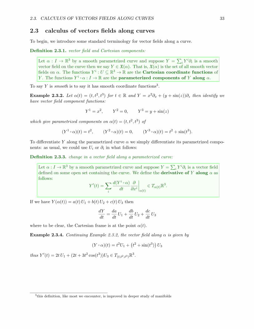
To begin, we introduce some standard terminology for vector fields along a curve.
Definition 2.3.1. vector field and Cartesian components:
Let α : I → R3 by a smooth parametrized curve and suppose Y =∑
i Yi∂i is a smooth
vector field on the curve then we say Y ∈ X(α). That is, X(α) is the set of all smooth vectorfields on α. The functions Y i : U ⊆ R3 → R are the Cartesian coordinate functions ofY . The functions Y i ◦α : I → R are the parameterized components of Y along α.
To say Y is smooth is to say it has smooth coordinate functions3.
Example 2.3.2. Let α(t) = (t, t2, t3) for t ∈ R and Y = x2∂x + (y + sin(z))∂z then identify wehave vector field component functions:
Y 1 = x2, Y 2 = 0, Y 3 = y + sin(z)
which give parametrized components on α(t) = (t, t2, t3) of
(Y 1 ◦α)(t) = t2, (Y 2 ◦α)(t) = 0, (Y 3 ◦α)(t) = t2 + sin(t3).
To differentiate Y along the parametrized curve α we simply differentiate its parametrized compo-nents: as usual, we could use Ui or ∂i in what follows:
Definition 2.3.3. change in a vector field along a parameterized curve:
Let α : I → R3 by a smooth parametrized curve and suppose Y =∑
i Yi∂i is a vector field
defined on some open set containing the curve. We define the derivative of Y along α asfollows:
Y ′(t) =∑i
d(Y i ◦α)
dt
∂
∂xi
∣∣∣∣α(t)
∈ Tα(t)R3.
If we have Y (α(t)) = a(t)U1 + b(t)U2 + c(t)U3 then
dY
dt=da
dtU1 +
db
dtU2 +
dc
dtU3
where to be clear, the Cartesian frame is at the point α(t).
Example 2.3.4. Continuing Example 2.3.2, the vector field along α is given by
(Y ◦α)(t) = t2U1 +(t2 + sin(t3)
)U3
thus Y ′(t) = 2t U1 + (2t+ 3t2 cos(t3))U3 ∈ T(t,t2,t3)R3.
3this definition, like most we encounter, is improved in deeper study of manifolds
34 CHAPTER 2. CURVES AND FRAMES
Proposition 2.3.5. calculus of vector fields on curves.
Let α is a smooth parametrized curve and Y,Z ∈ X(α) and c1, c2 ∈ R,
(i.)d
dt(c1Y + c2Z) = c1
dY
dt+ c2
dZ
dt,
(ii.)d
dt(Y •Z)(α(t)) =
dY
dt•Z(α(t)) + Y (α(t)) •
dZ
dt,
(iii.)d
dt(Y × Z) =
dY
dt× Z(α(t)) + Y (α(t))× dZ
dt.
Proof: if Y ◦α =∑i
aiUi and Z ◦α =∑i
biUi then (Y •Z) ◦α =∑i
aibi thus calculate:
d
dt(Y •Z) ◦α =
d
dt
∑i
aibi
=∑i
d
dt(aibi)
=∑i
[dai
dtbi + ai
dbi
dt
]=∑i
dai
dtbi +
∑i
aidbi
dt
=dY
dt•Z(α(t)) + Y (α(t)) •
dZ
dt.
Since (Y ×Z) ◦α =∑i,j,k
εijkaibjUk we can prove (3.) in a similar fashion. I leave (1.) to the reader. �
In Chapter 1 we studied how a given parametrized curve naturally generates an associated vectorfield which is known as the velocity of the curve. If we differentiate the velocity field along α thisgenerates the acceleration which is also a vector field along α.
Definition 2.3.6. acceleration of parametrized curve:
Let α : I → R3 by a smooth parametrized curve then define α′′(t) = ddt (α′(t) ). That is:
α′′(t) =∑i
d2(Y i ◦α)
dt2∂
∂xi
∣∣∣∣α(t)
∈ Tα(t)R3.
The definitions of acceleration and velocity we give in this section should be recognizable frommultivariate calculus, or university physics. However, the concept of differentiating a vector fieldalong the curve and fitting the acceleration in the context of that construction is probably new.
Example 2.3.7. Let α(t) = (t, t2, t3) for t ∈ R. Then
α′(t) = U1 + 2t U2 + 3t2 U3 & α′′(t) = 2U2 + 6t U3.
where both α′(t) and α′′(t) are in Tα(t)R3.

2.4. FRENET SERRET FRAME OF A CURVE 35
The concept of distant parallelism is fairly easy to grasp in Rn. In particular, we say (p, v) and(q, w) are distantly parallel if p 6= q and v •w = ||v|| ||w||. That is, for p 6= q, the vectors (p, v) and(q, w) are distantly parallel if there vector parts are parallel. For example, given a non-intersectingparametrized curve α, if a vector field Y has Y (α(t)) =
(c1∂x + c2∂y + c3∂z
)|α(t) for constants
c1, c2, c3 then Y (α(t1)) and Y (α(t2)) are distantly parallel.
Theorem 2.3.8.
Let α : I → R3 is a smooth parametrized curve,
(i.) α′ = 0 iff α(t) = p for all t ∈ I (that is, α is a point),
(ii.) α′′ = 0 iff α(t) = p+ tv for all t ∈ I (that is, α is a line),
(iii.) Let Y ∈ X(α) then the derivative of Y along α is zero iff Y ◦α = c1U1 + c2U2 + c3U3
for constants c1, c2, c3.
Proof of (1.): if α′ = 0 then for i = 1, 2, 3 we have dαi
dt = 0 for all t ∈ I. We assume I is connectedhence αi(t) = pi for all t ∈ I thus α(t) = p for all t ∈ I. Conversely α(t) = p clearly implies α′ = 0.
Proof of (2.): almost the same as (1.), just have to integrate twice in the forward direction andclearly α(t) = p+ tv for p, v ∈ R3 has α′′(t) = 0. I leave the details to the reader.
Proof of (3.): let Y ∈ X(α) have constant length along α. Suppose the derivative of Y along
α is zero. That is, suppose ddt(Y ◦α) = 0. Let (Y ◦α)i = ai then we are given dai
dt = 0 for t ∈ I.
Observe, for i = 1, 2, 3, dai
dt = 0 for all t ∈ I implies ai = ci for some constant ci. Therefore,Y ◦α = c1U1 + c2U2 + c3U3. Conversely, it is simple to see that Y ◦α = c1U1 + c2U2 + c3U3 forconstants c1, c2, c3 implies d
dt(Y ◦α)(t) = 0 hence Y ′ = 0. �
Given that Y ∈ X(α) has constant length along α we do have the equivalence: Y ′ = 0 iff Y (α(t1))is distantly parallel to Y (α(t2)). The addition of the assumption of constant length is needed sinceit is possible to have vector fields which are parallel along α but have variable length. For example,take α(t) = (t, t, t) for t ∈ [1, 2] and consider Y = xU1. We have Y (α(t)) = tU1 thus, for anyt ∈ [1, 2] the vector Y (α(t)) is distantly parallel4 to U1. However, Y ′ = U1 6= 0. In short, I arguepart (3.) of Lemma 2.3 on page 56 of O’neill (where no mention of Y ’s length is made) is falseunless we insist Y have constant length.
2.4 Frenet Serret frame of a curve
We have the necessary toys. Finally, let us play. We wish to find a frame along a curve. Linesare too boring, there is no nice way to pick a direction in the normal plane at a given point. Forα(t) = p+ tv it is easy enough to see α′(t) = (p+ tv, v), but, beyond the direction vector v, how towe find another characteristic vector for the line? This problem is either too easy or too hard forus, so, we set it aside and assume in the remainder of this section we have a non-linear,regular, parametrized curve parametrized by arclength. That is, we have a non-linear,unit-speed curve. We wish to find a frame along α.
4you might notice distant parallelism is an equivalence relation

36 CHAPTER 2. CURVES AND FRAMES
Our goal is to find a frame E1, E2, E3 along α; that is E1, E2, E3 ∈ X(α) for which E1, E2, E3 formsan orthonormal basis for Tα(t)R3 at each t ∈ dom(α). We’ll start with the velocity of the curve.Let us denote the unit-tangent field by T = α′(s) then T •T = ||α′(s)|| = 1. Next, we need tofind another vector field along α. Notice T ′ •T + T •T ′ = 0 on α(t) hence T ′ is orthogonal to Talong the curve. However, ||T ′|| is not generally 1 thus we must normalize and define the normalvector field by N = 1
||T ′||T′. In fact, geometrically, the change in the tangent vector along the curve
measures how the curve is changing direction. We define:
Definition 2.4.1. curvature of smooth curve.
Suppose α is an arclength-parametrized curve then the curvature of α is given by κ = ||T ′||.
Notice, if α′′ = 0 then T ′ = α′′ = 0 hence κ = 0 for a line. We are primarily interested in thecase κ > 0. Observe, by construction, N •N = 1 and N •T = 0. Finally, we define the binormalB = T ×N . Clearly, B •T = 0 and B •N = 0 hence ||B|| = ||T ||||N || sin(90o) = 1. Thus T,N,Bforms a positively oriented frame along α known as the Frenet frame of α. The term positivelyoriented refers to the fact that the triple T,N,B respects the right-hand-rule as B = T ×N . Thetangent and normal vector fields to the curve both are tangent to the so-called osculating plane.This makes the binormal a vector which is perpendicular to the osculating plane. That is, thebinormal forms the normal to the osculating plane. We’ll see in the proof of the proposition tofollow that there is a function τ which governs the evolution of B with the curve. That function iscalled the torsion. In short, it measures the tendency of the curve to bend off its osculating plane.
Theorem 2.4.2. Frenet Serret Equations.
Let α be a unit-speed, non-linear curve and define T = dαds and N = 1
||T ′||dTds and B = T ×N
then there exists a function τ for which:
dT
ds= κN
dN
ds= −κT + τ B
dB
ds= −τN
Proof: begin by noting κ = ||T ′|| hence N = 1κdTds hence dT
ds = κN is just the definition of κ. Theother two equations require a bit more effort.
We wish to show T,N,B forms a frame along α. To verify this, observe T •T = ||α′(s)|| = 1 as αis given to be unit-speed. Differentiate by part (ii.) of Proposition 2.3.5,
T •T = 1 ⇒ T ′ •T + T •T ′ = 2T •T ′ = 0 ⇒ T •
[T ′
||T ′||
]= T •N = 0.
By construction, N •N = 1||T ′||2T
′ •T ′ = 1. By properties of the cross-product, B is orthogonal to
both N and T as B = T ×N . Finally, ||B|| = ||T ×N || = ||T ||||N || sin(90o) = 1 hence B •B = 1.Sorry to be redundant here, but, to be safe I want all of this here.
Notice, N ′ and B′ are vector fields along α by their construction. It follows we can expand eachof them in terms of the frame T,N,B along α. Moreover, the components with respect to this
2.4. FRENET SERRET FRAME OF A CURVE 37
orthonormal basis are simply given by dot-products. Begin with B′ we have:
B′ = (B′ •T )T + (B′ •N)N + (B′ •B)B ?B
notice B •B = 1 implies B′ •B = 0. Also, B •T = 0 implies
B′ •T +B •T ′ = 0 ⇒ B′ •T = −B •T ′ = −B • (κN) = −κB •N = 0.
We deduce from ?B that B′ = (B′ •N)N . Let τ = −B′ •N and we obtain dBds = −τN .
Once more use that T,N,B forms a frame on α and N ′ ∈ X(α),
N ′ = (N ′ •T )T + (N ′ •N)N + (N ′ •B)B ?N
As usual, N •N = 1 implies N ′ •N = 0. On the other hand, N •T = 0 yields,
N ′ •T +N •T ′ = 0 ⇒ N ′ •T = −T ′ •N = −κN •N = −κ.
Whereas, N •B = 0 differentiates to yield:
N ′ •B +N •B′ = 0 ⇒ N ′ •B = −N •B′ = −N • (−τN) = τ.
Therefore, returing to ?N we find dNdS = −κT + τB. �
This proof is really not that complicated. The boxed equations are immediate once we recognizeT,N,B forms a frame. Then, we just used part (ii.) of Proposition 2.3.5 repeatedly to cut thecomponents of the boxed equation down to size. We have shown the definition of torsion to followis well-posed:
Definition 2.4.3. torsion of smooth curve.
Let α is an arclength-parametrized curve then the torsion of α is given by τ = −N • dBds .
Example 2.4.4. Consider the helix defined by R,m > 0 and
α(s) = (R cos(ks), R sin(ks),mks)
for s ∈ R and k = 1/√R2 +m2. Calculate,
α′(s) = −kR sin(ks)U1 + kR cos(ks)U2 +mkU3
thus ||α′(s)|| = k√R2 +m2 = 1. It follows T = α′. Differentiate α′ to obtain:
T ′(s) = α′′(s) = −k2R cos(ks)U1 − k2R sin(ks)U2
We find ||T ′(s)|| = k2R hence κ = R/(R2 +m2). Note N = − cos(ks)U1 − sin(ks)U2 thus
B = T ×N =(−kR sin(ks)U1 + kR cos(ks)U2 +mkU3
)×(− cos(ks)U1 − sin(ks)U2
)= mk sin(ks)U1 −mk cos(ks)U2 + kRU3.
As a quick check on the calculation, notice B •N = 0 and B •T = 0. Calculate,
dB
ds=
d
ds[mk sin(ks)U1 −mk cos(ks)U2 + kRU3]
= mk2 cos(ks)U1 +mk2 sin(ks)U2
Thus dBds•N = −mk2 thus τ = mk2 = m/(m2 +R2).

38 CHAPTER 2. CURVES AND FRAMES
The nice thing about the helix example is we see nonzero curvature and torsion. Moreover, wecan see other features in particular limits of the general formulas. For example, if m = 0 thenα(s) = (R cos(ks), R sin(ks), 0) is just a circle and the torsion τ = 0 as B = U3. A circle is a planarcurve and the vanishing torsion reflects this fact. Also, when m = 0 we have κ = 1/R. We find thecurvature is large when R is small.
Generally, if a curve lies in a plane then surely T and N are tangent to the plane. But, then thatgives B is colinear to the normal of the plane which implies B is constant hence τ = 0. Conversely,if τ = 0 for a curve then we have B is constant along the curve which implies T,N are alwaysparallel to a plane with B as a normal. So, it seems plausible that a curve is planar iff it hasvanishing torsion. That said, we should be a bit more precise:
Theorem 2.4.5. no torsion, non-linear curves are planar
Let α be a unit-speed, non-linear curve then α is a planar curve iff τ = 0.
Proof ( ⇒ ) : if the parametrized curve α : I → R3 lies on a plane with normal V then andsuppose so ∈ I. Then α(so) is a point on the plane and we have that γ(s) •V = 0 for all s ∈ Iwhere γ(s) = α(s)− α(so) is the secant line from so to s on the given curve. By the product ruleand the fact that V is constant we have γ′(s) •V = 0 hence T •V = 0 and differentiating againyields T ′ •V = κN •V = 0 hence N •V = 0 as α is non-linear gives κ > 0. We find V is orthogonalto both T and N for each s ∈ I hence V is colinear with B at each s ∈ I and as B 6= 0 and V 6= 0there must exist k 6= 0 for which B = kV . Thus B′ = 0 and we derive τ = −B′ •N = 0.
Proof ( ⇐ ) : suppose τ(s) = 0 for all s ∈ I where so ∈ I and α : I → R3 is a non-linearregular curve. Notice B′ = −τN = 0 for all s ∈ I hence B(s) = B(so) for all s ∈ I. We expectthat B(so) serves as the normal to the plane in which the curve evolves. Thus define a functionwhich if identically zero will show that the curve lies in a plane with point α(so) and normal B(so).Following O’neill5,
f(s) = [α(s)− α(so)] •B(so) ⇒ df
ds= α′(s) •B(so) = T (s) •B(s) = 0
for all s ∈ I however f(so) = 0 thus f(s) = 0 for all s ∈ I and so we find the curve is planar withthe constant binormal serving as the normal to the plane of motion. �
It is instructive to consider how the curvature and torsion locally approximate the geometry of asmooth regular unit-speed curve. Taylor’s theorem gives, for some point so in the domain of α,
α(s) ≈ α(so) + sα′(so) +s2
2α′′(so) +
s3
6α′′′(so) + · · · ?
Note α′(so) = T (so) and for our convenience let us denote T (so) = To hence identify first twoterms parametrize the tangent line at α(so) by α(so) + sTo. Next, by the Frenet Serret equationfor T ′ = α′′ we see
α′′(so) = T ′(so) = κ(so)N(so)
5notice that α(s) − α(so) is naturally associated with the directed line-segment in R3 from α(so) to α(s). Weattach that directed line-segment to α(so) as to make the dot-product with B(so) ∈ Tα(so)R
3 reasonable. Since littleis gained by making these identifications explicit in the proof we follow O’neill and most authors and omit commentssuch as these in most places (except here I suppose)
2.4. FRENET SERRET FRAME OF A CURVE 39
let κ(so) = κo and N(so) = No. Thus ? reads
α(s) ≈ α(so) + sTo +1
2s2κoNo +
s3
6α′′′(so) + · · ·
Torsion contributes to the third derivative term. Let’s see how. Note, α′′ = T ′ = κN thus
α′′′ =dκ
dsN + κN ′ =
dκ
dsN + κ(−κT + τB) = −κ2T +
dκ
dsN + κτB
thus, to third order in arclength,
α(s) ≈ α(so) +(s− 1
6s3κ2o
)To +
(12s
2κo + 16s
3κ′o)No + 1
6s3κoτoBo + · · ·
To just second order in s we have motion in a plane spanned by To, No. Suppose we let x, y be theTo, No coordinates respective then if α(so) = 0 we can express
x = s y =1
2s2κo ⇒ y =
1
2κx2.
Thus, the motion follows a parabola with slope κx. We can approximate the motion of the curve atany point in this fashion. Alternatively, we can fit a circle locally to the curve. The circle which fitsat α(so) is called the osculating circle. The osculating circle has radius 1/κo. In x, y coordinatesas described above, the equation of the osculating circle is:
x2 +
(y − 1
κo
)2
=1
κ2o
.
See the background of http://www.supermath.info/MultivariateCalculus.html for a animated pic-ture of an osculating circle attached to a rather twisty space curve. Thanks to my brother Billfor the Maple code. You can read about the osculating sphere in Theorem 2.10 on page 22-23 ofWolfgang Kuhnel’s Differential Geometry: Curves-Surfaces-Manifolds.
Suppose the curvature is constant along some segment of a unit-speed regular curve. If the curvatureis constantly zero then is a part of a line by part (ii.) of Theorem 2.3.8. On the other hand, ifκ(s) = c > 0 for all s in some interval then the osculating circles along the curve share the sameradius and we might hope they are in fact the same circle. As it happens, we also need the curveto be planar, so the assumption τ = 0 is added below:
Theorem 2.4.6. constant curvature κ 6= 0 curve follows circle of radius 1/κ
Let α be a unit-speed, non-linear curve with constant curvature κ(s) = κo 6= 0 and τ(s) = 0for all s ∈ I then α(s) follows a circle of radius 1/κo.
Proof 1: Let α be a unit-speed, non-linear curve with constant curvature κ(s) = κo 6= 0 andτ(s) = 0 for all s ∈ I. Let so ∈ I and denote To, No to be T (s), N(s) with s = so. We expect thecircle which the curve follows has radius R = 1/κo thus C = α(so) + RNo should be the center ofthe circle. Points along the circle should be equidistant from C. As τ(s) = 0 we know α(s) falls onthe plane with point α(so) and normal B(so). It follows there are functions a(s), b(s) for which
α(s) = α(so) + a(s)To + b(s)No
40 CHAPTER 2. CURVES AND FRAMES
Thus,
α(s)− C = α(so) + a(s)To + b(s)No − [α(so) +RNo]
= a(s)To + (b(s)−R)No
But, α′(s) = a′(s)To + b′(s)No and α′′(s) = a′′(s)To + b′′(s)No. Since α′(s) = T (s) and α′′(s) =T ′(s) = κ(s)N(s) = κoN(s) we have:
a′′(s)To + b′′(s)No = κoN(s)
differentiating yields
a′′′(s)To + b′′′(s)No = κoN′(s) = κo(−κT + τB) = −κ2
oT (s)
however, −κ2oT (s) = −κ2
o[a′(s)To + b′(s)No] thus the equation above yields
(a′′′ + κ2oa′)To + (b′′′ + κ2
ob′)No = 0
which means a, b are solutions to the following constant coefficient ODEs,
a′′′ + κ2oa′ = 0, b′′′ + κ2
ob′ = 0
Solutions below follow from standard arguments in the introductory DEqns course,
a(t) = c1 + c2 cos(κos) + c3 sin(κos), b(t) = c4 + c5 cos(κos) + c6 sin(κos)
Next, we could apply the initial data implicit within the construction of a(s) and b(s) and seek toshow ||α(s)− C|| = 1/κo. I will stop here as it turns out this proof is needlessly complicated. �
The basic idea of the proof above is often successful. And, sometimes, we have no choice but towork through a problem in differential equations paired with difficult algebra. But, the proof whichfollows is certainly an easier approach. Following O’neill:
Proof 2: Let α be a unit-speed, non-linear curve with constant curvature κ(s) = κo 6= 0 andτ(s) = 0 for all s ∈ I. Consider, at any point along the curve, the normal vector should pointtowards the center C of the conjectured circle. That is, C −RN(s) = α(s) for R = 1/κo. Define
γ(s) = α(s) +RN(s)
differentiating we obtain:
γ′(s) = α′(s) +RN ′(s) = T (s)−RκoT (s) = T (s)− T (s) = 0
therefore γ′(s) = 0 for all s ∈ I. Let so ∈ I and observe γ(so) = α(so) + RN(so) = γ(s) for alls ∈ I. Thus identify C = α(so) +RN(so) is the fixed center of the circle. Hence α(s)−C = RN(s)for all s ∈ I and so ||α(s)−C|| = R for all s ∈ I. Therefore, α is on a circle of radius R = 1/κo. �

2.4. FRENET SERRET FRAME OF A CURVE 41
Example 2.4.7. If a curve is on a sphere then it is at least as curved as a great circle on thesphere. To see this, consider α : I → R3 a unit-speed regular curve on the sphere with center C andradius R. We are given ||α(s)− C|| = R for all s ∈ I. Of course,
(α− C) • (α− C) = R2
hence, as α′ = T , the product rule and commutativity of the dot-product yield
2T • (α− C) = 0.
Divide by two and differentiating once more,
T ′ • (α− C) + T •T = 0.
But, T ′ = κN and T •T = 1 thus
κN • (α− C) + 1 = 0 ⇒ −1/κ = N • (α− C)
thus, by Cauchy-Schwarz inequality and facts ||N || = 1 and ||α− C|| = R,
1
κ≤ R
Therefore, κ ≥ 1/R. The smallest curvature possible for a curve on a sphere is the case the curveis a great circle. A great circle on a sphere of radius R is naturally a circle of radius R and givenour previous work on the helix example we know κ = 1/R for the circle.
2.4.1 the non unit-speed case
Up to this point, we have studied curves with unit-speed. In other words, we have thus far studiedthe Frenet Serret theory for arclength parametrized curves. There are curves for which no such pa-rameterization can be reasonable expressed, yet, relatively simple formulas are known for variablespeed parameterizations.
Consider α : I → R3 a regular smooth parameterized curve. Also, let α : J → R3 be thereparametrization of α by the arclength function s : I → J . In particular, α(t) = α(s(t)) foreach t ∈ I. If we define T , N , B, κ and τ as discussed earlier in this section then T,N,B, κ and τin the t-domain are defined by reparametrization:
T (t) = T (s(t)), N(t) = N(s(t)), B(t) = B(s(t)), κ(t) = κ(s(t)), τ(t) = τ(s(t)).
We denote the speed by v where v = dsdt = ||α′(t)||. The chain-rule yields:
α′(t) =d
dt[α(s(t))] = α′(s(t))
ds
dt= vT (s(t)) ?
likewise,
T ′(t) =d
dt
[T (s(t))
]= T ′(s(t))
ds
dt= v(t)κ(s(t))N(s(t)) = v(t)κ(t)N(t).
Thus, the Frenet Serret equation for a non-unit-speed curve is modified todT
dt= vκN . The same
argument applies to the derivative of N and B hence:
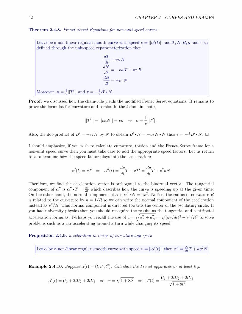
42 CHAPTER 2. CURVES AND FRAMES
Theorem 2.4.8. Frenet Serret Equations for non-unit speed curves.
Let α be a non-linear regular smooth curve with speed v = ||α′(t)|| and T,N,B, κ and τ asdefined through the unit-speed reparameterization then
dT
dt= vκN
dN
dt= −vκT + vτ B
dB
dt= −vτN
Moreover, κ = 1v ||T
′|| and τ = − 1vB′ •N .
Proof: we discussed how the chain-rule yields the modified Frenet Serret equations. It remains toprove the formulas for curvature and torsion in the t-domain: note,
||T ′|| = ||vκN || = vκ ⇒ κ =1
v||T ′||.
Also, the dot-product of B′ = −vτN by N to obtain B′ •N = −vτN •N thus τ = − 1vB′ •N . �
I should emphasize, if you wish to calculate curvature, torsion and the Frenet Serret frame for anon-unit speed curve then you must take care to add the appropriate speed factors. Let us returnto ? to examine how the speed factor plays into the acceleration:
α′(t) = vT ⇒ α′′(t) =dv
dtT + vT ′ =
dv
dtT + v2κN
Therefore, we find the acceleration vector is orthogonal to the binormal vector. The tangentialcomponent of α′′ is α′′ •T = dv
dt which describes how the curve is speeding up at the given time.On the other hand, the normal component of α is α′′ •N = κv2. Notice, the radius of curvature Ris related to the curvature by κ = 1/R so we can write the normal component of the accelerationinstead as v2/R. This normal component is directed towards the center of the osculating circle. Ifyou had university physics then you should recognize the results as the tangential and centripetal
acceleration formulas. Perhaps you recall the use of a =√a2T + a2
N =√
(dv/dt)2 + v4/R2 to solve
problems such as a car accelerating around a turn while changing its speed.
Proposition 2.4.9. acceleration in terms of curvature and speed
Let α be a non-linear regular smooth curve with speed v = ||α′(t)|| then α′′ = dvdtT + κv2N
Example 2.4.10. Suppose α(t) = (t, t2, t2). Calculate the Frenet apparatus or at least try.
α′(t) = U1 + 2tU2 + 2tU3 ⇒ v =√
1 + 8t2 ⇒ T (t) =U1 + 2tU2 + 2tU3√
1 + 8t2

2.4. FRENET SERRET FRAME OF A CURVE 43
Thus,
T ′(t) =2U2 + 2U3√
1 + 8t2− 1
2
U1 + 2tU2 + 2tU3
(√
1 + 8t2)3(16t)
=2(1 + 8t2)(U2 + U3)− 8t(U1 + 2tU2 + 2tU3)
(√
1 + 8t2)3
=−8tU1 + 2U2 + 2U3
(√
1 + 8t2)3
=2
(√
1 + 8t2)3
(−4tU1 + U2 + U3
)Thus,
κ(t) =1
v||T ′(t)|| = 1√
1 + 8t22√
16t2 + 2
(√
1 + 8t2)3⇒ κ(t) =
2√
16t2 + 2
(1 + 8t2)2.
I leave the calculation of B(t) and the torsion to the reader. Also, I invite the reader to verify thatapplication of Theorem 2.4.9 to the acceleration of the given curve:
α′′ = 2U2 + 2U3 =−8t
(√
1 + 8t2)3T (t) +
2√
16t2 + 2
1 + 8t2N(t)
You can see problems such as the last example are good candidates for CAS assistance. Also, thetheorem below may be helpful. You may have noticed I already assumed we could calculate T (t)as given below:
Theorem 2.4.11. slick formulas for the Frenet apparatus
Let α be a non-linear regular smooth curve with speed v = ||α′(t)|| and T,N,B, κ and τ asdefined through the unit-speed reparameterization then
T =α′
||α′||, B =
α′ × α′′
||α′ × α′′||, N = B × T,
κ =||α′ × α′′||||α′||3
, τ =(α′ × α′′) •α′′′
||α′ × α′′||2
Proof: see pages 72-73 of O’neill. �
O’neill also give a nice example which showcases how these formulas work on page 73. In addition,O’neill proves part of the following assertions. I leave these to the reader, but, I thought includingthem would be wise. It is likely I prove part of this in lecture.
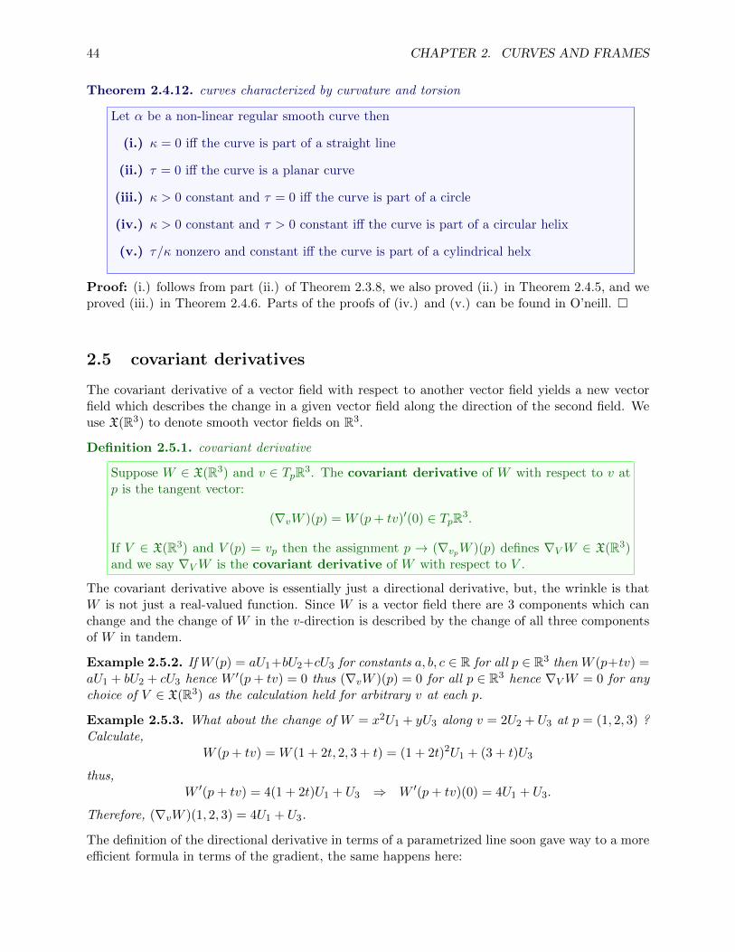
44 CHAPTER 2. CURVES AND FRAMES
Theorem 2.4.12. curves characterized by curvature and torsion
Let α be a non-linear regular smooth curve then
(i.) κ = 0 iff the curve is part of a straight line
(ii.) τ = 0 iff the curve is a planar curve
(iii.) κ > 0 constant and τ = 0 iff the curve is part of a circle
(iv.) κ > 0 constant and τ > 0 constant iff the curve is part of a circular helix
(v.) τ/κ nonzero and constant iff the curve is part of a cylindrical helx
Proof: (i.) follows from part (ii.) of Theorem 2.3.8, we also proved (ii.) in Theorem 2.4.5, and weproved (iii.) in Theorem 2.4.6. Parts of the proofs of (iv.) and (v.) can be found in O’neill. �
2.5 covariant derivatives
The covariant derivative of a vector field with respect to another vector field yields a new vectorfield which describes the change in a given vector field along the direction of the second field. Weuse X(R3) to denote smooth vector fields on R3.
Definition 2.5.1. covariant derivative
Suppose W ∈ X(R3) and v ∈ TpR3. The covariant derivative of W with respect to v atp is the tangent vector:
(∇vW )(p) = W (p+ tv)′(0) ∈ TpR3.
If V ∈ X(R3) and V (p) = vp then the assignment p → (∇vpW )(p) defines ∇VW ∈ X(R3)and we say ∇VW is the covariant derivative of W with respect to V .
The covariant derivative above is essentially just a directional derivative, but, the wrinkle is thatW is not just a real-valued function. Since W is a vector field there are 3 components which canchange and the change of W in the v-direction is described by the change of all three componentsof W in tandem.
Example 2.5.2. If W (p) = aU1+bU2+cU3 for constants a, b, c ∈ R for all p ∈ R3 then W (p+tv) =aU1 + bU2 + cU3 hence W ′(p+ tv) = 0 thus (∇vW )(p) = 0 for all p ∈ R3 hence ∇VW = 0 for anychoice of V ∈ X(R3) as the calculation held for arbitrary v at each p.
Example 2.5.3. What about the change of W = x2U1 + yU3 along v = 2U2 +U3 at p = (1, 2, 3) ?Calculate,
W (p+ tv) = W (1 + 2t, 2, 3 + t) = (1 + 2t)2U1 + (3 + t)U3
thus,W ′(p+ tv) = 4(1 + 2t)U1 + U3 ⇒ W ′(p+ tv)(0) = 4U1 + U3.
Therefore, (∇vW )(1, 2, 3) = 4U1 + U3.
The definition of the directional derivative in terms of a parametrized line soon gave way to a moreefficient formula in terms of the gradient, the same happens here:
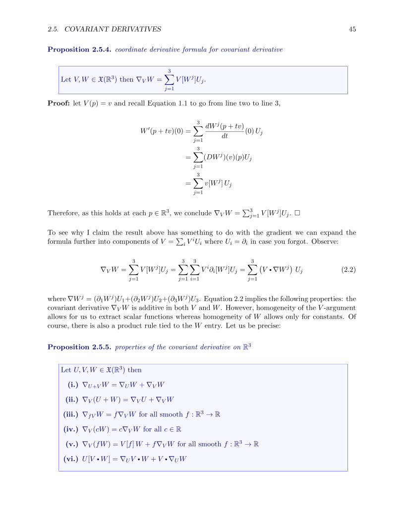
2.5. COVARIANT DERIVATIVES 45
Proposition 2.5.4. coordinate derivative formula for covariant derivative
Let V,W ∈ X(R3) then ∇VW =3∑j=1
V [W j ]Uj .
Proof: let V (p) = v and recall Equation 1.1 to go from line two to line 3,
W ′(p+ tv)(0) =3∑j=1
dW j(p+ tv)
dt(0)Uj
=
3∑j=1
(DW j)(v)(p)Uj
=3∑j=1
v[W j ]Uj
Therefore, as this holds at each p ∈ R3, we conclude ∇VW =∑3
j=1 V [W j ]Uj . �
To see why I claim the result above has something to do with the gradient we can expand theformula further into components of V =
∑i V
iUi where Ui = ∂i in case you forgot. Observe:
∇VW =3∑j=1
V [W j ]Uj =3∑j=1
3∑i=1
V i∂i[Wj ]Uj =
3∑j=1
(V •∇W j
)Uj (2.2)
where∇W j = (∂1Wj)U1+(∂2W
j)U2+(∂3Wj)U3. Equation 2.2 implies the following properties: the
covariant derivative ∇VW is additive in both V and W . However, homogeneity of the V -argumentallows for us to extract scalar functions whereas homogeneity of W allows only for constants. Ofcourse, there is also a product rule tied to the W entry. Let us be precise:
Proposition 2.5.5. properties of the covariant derivative on R3
Let U, V,W ∈ X(R3) then
(i.) ∇U+VW = ∇UW +∇VW
(ii.) ∇V (U +W ) = ∇V U +∇VW
(iii.) ∇fVW = f∇VW for all smooth f : R3 → R
(iv.) ∇V (cW ) = c∇VW for all c ∈ R
(v.) ∇V (fW ) = V [f ]W + f∇VW for all smooth f : R3 → R
(vi.) U [V •W ] = ∇UV •W + V •∇UW
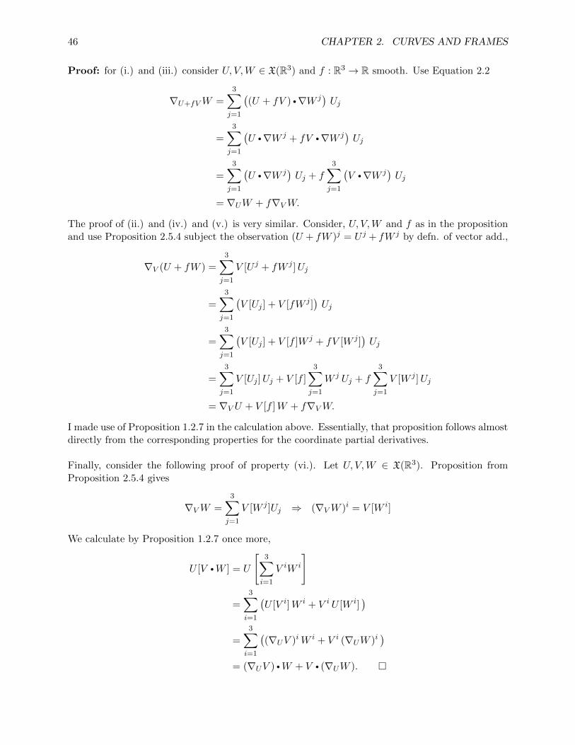
46 CHAPTER 2. CURVES AND FRAMES
Proof: for (i.) and (iii.) consider U, V,W ∈ X(R3) and f : R3 → R smooth. Use Equation 2.2
∇U+fVW =
3∑j=1
((U + fV ) •∇W j
)Uj
=3∑j=1
(U •∇W j + fV •∇W j
)Uj
=
3∑j=1
(U •∇W j
)Uj + f
3∑j=1
(V •∇W j
)Uj
= ∇UW + f∇VW.
The proof of (ii.) and (iv.) and (v.) is very similar. Consider, U, V,W and f as in the propositionand use Proposition 2.5.4 subject the observation (U + fW )j = U j + fW j by defn. of vector add.,
∇V (U + fW ) =3∑j=1
V [U j + fW j ]Uj
=
3∑j=1
(V [Uj ] + V [fW j ]
)Uj
=3∑j=1
(V [Uj ] + V [f ]W j + fV [W j ]
)Uj
=
3∑j=1
V [Uj ]Uj + V [f ]
3∑j=1
W j Uj + f
3∑j=1
V [W j ]Uj
= ∇V U + V [f ]W + f∇VW.
I made use of Proposition 1.2.7 in the calculation above. Essentially, that proposition follows almostdirectly from the corresponding properties for the coordinate partial derivatives.
Finally, consider the following proof of property (vi.). Let U, V,W ∈ X(R3). Proposition fromProposition 2.5.4 gives
∇VW =3∑j=1
V [W j ]Uj ⇒ (∇VW )i = V [W i]
We calculate by Proposition 1.2.7 once more,
U [V •W ] = U
[3∑i=1
V iW i
]
=
3∑i=1
(U [V i]W i + V i U [W i]
)=
3∑i=1
((∇UV )iW i + V i (∇UW )i
)= (∇UV ) •W + V • (∇UW ). �
2.5. COVARIANT DERIVATIVES 47
Of course, all the calculations above are to be done at a point p, but, as the identity holds generallywe obtain statements about functions and vector fields. I decided the proofs without explicit pointsare easier to follow. Perhaps the same is true for examples: incidentally, it is useful to write theformula for the covariant derivative in explicit detail for the sake of the example which follows:
∇VW = V [W 1]U1 + V [W 2]U2 + V [W 3]U3.
Example 2.5.6. Let V = xU1 +y2U2 +z3U3 and W = yzU1 +xyU3. Recall our notation U1, U2, U3
masks the fact that these are derivations; U1 = ∂x, U2 = ∂y and U3 = ∂z thus:
V [yz] = x∂x[yz] + y2∂y[yz] + z3∂z[yz] = y2z + z3y.
V [xy] = x∂x[xy] + y2∂y[xy] + z3∂z[xy] = xy + y2x.
Therefore, as W 1 = yz and W 3 = xy we find
∇VW = V [yz]U1 + V [xy]U3 = (y2z + z3y)U1 + (xy + y2x)U3.
Example 2.5.7. Calculate ∇V V . To calculate ∇V V it may be instructive to use property (vi.),
V [V •V ] = (∇V V ) •V + V • (∇V V ).
Thus, as V [f2] = 2fV [f ] for smooth f we have:
(∇V V ) •V =1
2V [||V ||2] = ||V ||V [||V ||]
Divide by ||V || to see the component of ∇V V in the V -direction is simply V [||V ||]. As a particularapplication of this calculation, notice if the vector field is of constant length then V [||V ||] = 0 whichmeans that V does not change in the V (p) direction at p.
Finally, a word of caution, the idea of covariant differentiation shown in this section is just thefirst chapter in a larger story. More generally, the covariant derivative is tied to something calleda connection on a fiber bundle. Roughly, this extends the idea of distant parallelism to generalspaces. I suppose I should also mention, in General Relativity there is a covariant derivative withrespect to the metric connection which is used define geodesics. General relativity claims particlesfollowing geodesics in the spacetime manifold explains gravity in nature. In any event, for nowwe study the covariant derivative in R3. We later study a different covariant derivative associatedwith the calculus of a surface. Next, we continue to study the covariant derivative, but, with otherpossible non-Cartesian frames in R3.
48 CHAPTER 2. CURVES AND FRAMES
2.6 frames and connection forms
The covariant derivative of a vector field in Cartesian coordinate simply involves partial derivativesof coordinates. In this section we study how to calculate ∇VW with respect to a non-constantframe for R3. In addition to the derivative terms we saw in the last section there are new termscorresponding to nontrivial connection coefficients. The connection coefficients of a given framethen allow us to somewhat indirectly study the geometry of objects to which the frame is naturallyfit. For example, the curvature and torsion played the role of connection coefficients for the curveto which we fit the T,N,B frame. However, that is not quite the right picture as we intend to fitframes to surfaces. We will explain in this section that the connection coefficients are naturally iden-tified with a matrix of one-forms. Ultimately, the exterior calculus of these matrix-valued one-forms
If {E1, E2, E3} is a frame for R3 and V ∈ X(R3) then there exist functions f1, f2, f3 called thecomponents of V with respect to the frame {E1, E2, E3}
V = f1E1 + f2E2 + f3E3
Orthonormality of the frame shows the component functions are calculated from:
f j = V •Ej
Suppose V,W ∈ X(R3) where V =∑f iEi and W =
∑j g
jEj . Calculate, by Proposition 2.5.5,
∇VW = ∇∑f iEi
( ∑j
gjEj)
=∑i,j
f i∇Ei(gjEj
)=∑i,j
f i[Ei[g
j ]Ej + gj∇Ei(Ej)]
=∑j
V [gj ]Ej︸ ︷︷ ︸I.
+∑i,j
f igj∇Ei(Ej)︸ ︷︷ ︸II.
Recall, in terms of the Cartesian frame U1, U2, U3 if V =∑
i ViUi and W =
∑jW
jUj then
∇VW =∑j
V [W j ]Uj which resembles term (I.). In comparison, there is no type-II. term as should
be expected since Ui is contant hence ∇Ui(Uj) = 0.
Definition 2.6.1. connection forms6
If E1, E2, E3 is a frame for R3 then define ωij(p) ∈ (TpR3)∗ by
ωij(v) = (∇vEi ) •Ej(p)
for each v ∈ TpR3. That is, ωij is a differential one-form on R3 defined by the assignmentp 7→ ωij(p) for each p ∈ R3.
Half of the proposition below is a simple consquence of Equation 2.1.
6I was tempted to introduce structure functions Ckij = Ek •∇Ei(Ej), but, I behave. See page 202-203 ofManifolds, Tensors and Forms: An Introduction for Mathematicians and Physicsts by Renteln if you wish to readmore in that direction. In particular, he relates the structure functions to the Christoffel symbols. This approach

2.6. FRAMES AND CONNECTION FORMS 49
Proposition 2.6.2. properties of the covariant derivative on R3
Let {E1, E2, E3} be a frame on R3 then ωij = −ωji and ∇VEi =3∑j=1
ωij(V )Ej .
Proof: By a slight modification of Example 2.5.7, consider:
V [Ei •Ej ] = (∇VEi) •Ej + Ei • (∇VEj) ⇒ 0 = ωij(V ) + ωji(V )
for all V hence ωij = −ωji. Next, note ωij(V ) = (∇VEi) •Ej is the j-th component of ∇VEi in the
{E1, E2, E3} frame. If W = ∇VEi then W =∑
j(W •Ej)Ej . Therefore, ∇VEi =3∑j=1
ωij(V )Ej . �
It may be useful to express these explicitly:
∇VE1 = ω12(V )E1 + ω13(V )E3
∇VE2 = −ω12(V )E1 + ω23(V )E3
∇VE3 = −ω13(V )E1 − ω23(V )E2
We can arrange the differential forms ωij into a matrix ω
ω =
0 ω12 ω13
−ω12 0 ω23
−ω13 −ω23 0
This is a matrix of one-forms. Let us pause to develop the theory of matrices of forms over Rn
2.6.1 on matrices of differential forms
O’neill does not write ∧ for A ∧B I write below. But, I’d rather write a few wedges to emphasizethe nature of the calculation. Essentially, the definition below just replaces the ordinary productof real numbers in the usual matrix algebra with a wedge product of forms.
Definition 2.6.3. exterior algebra and calculus of matrices of forms:
Let Aik be a p-form and Bkj be a q-form for 1 ≤ i ≤ m, 1 ≤ k ≤ r and 1 ≤ j ≤ n then wesay A is an m × r matrix of p-forms and B is a r × n matrix of q-forms. Then we say Aand B are multipliable and define the m× n-matrix of (p+ q)-forms A ∧B by:
(A ∧B)ij =
r∑k=1
Aik ∧Bkj .
Likewise, we denote the exterior derivative of A by dA which is defined to be the m× r-matrix of (p+ 1)-forms given by (dA)ik = dAik.
We also denote, A =∑
i,k AikEik and B =∑
k,j BkjEkj where (Eij)lm = δilδjm. The standard-matrix-basis Eij is at times very useful for proofs and general questions. Furthermore, we defineAT in the usual manner; (AT )ij = Aji. Likewise, addition and substraction of forms as well asmultiplication by smooth functions are naturally defined.
50 CHAPTER 2. CURVES AND FRAMES
Example 2.6.4. Let A =
[dx dydz z2dy + y2dz
]and B =
[dx+ dy 0z2dy dx+ dz
]then
A ∧B =
[dx dydz z2dy + y2dz
]∧[dx+ dy 0z2dy dx+ dz
]=
[dx ∧ (dx+ dy) + dy ∧ z2dy dx ∧ 0 + dy ∧ (dx+ dz)
dz ∧ (dx+ dy) + (z2dy + y2dz) ∧ z2dy dz ∧ 0 + (z2dy + y2dz) ∧ (dx+ dz)
]=
[dx ∧ dy −dx ∧ dy + dy ∧ dz
dz ∧ dx− dy ∧ dz + y2z2dz ∧ dy z2(dy ∧ dz − dx ∧ dy) + y2dz ∧ dx
]The last step I included just to illustrate one way to simplify the answer. Also, calculate:
dA =
[0 00 2(y − z)dy ∧ dz
]& dB =
[0 0
2zdz ∧ dy 0
].
Observe, we can reasonably express these as matrix-valued two-forms; dA = (2(y − z)dy ∧ dz)E22
and dB = (2zdz ∧ dy)E21.
Proposition 2.6.5. product rule for matrices of forms
Let A be a matrix of p-forms andB be a matrix of q-forms and suppose A,B are multipliablethen
d(A ∧B) = dA ∧B + (−1)pA ∧ dB.
Proof: consider,
d(A ∧B)ij = d
(∑k
Aik ∧Bkj
): defn. of A ∧B
=∑k
d (Aik ∧Bkj) : additivity of d
=∑k
(dAik ∧Bkj + (−1)pAik ∧ dBkj) : by Prop. 1.3.3
= (dA ∧B + (−1)pA ∧ dB)ij
Therefore, as the above holds for all i, j, we conclude d(A ∧B) = dA ∧B + (−1)pA ∧ dB �
Of course, we probably could spend much more time and effort working out general results aboutthe exterior calculus of forms of matrices. For example, I invite the reader to verify associativity(A∧B)∧C = A∧ (B∧C). I wil behave and get back on task now. We are mainly interested in theattitude matrix of Definition 2.2.11. In Theorem 2.2.12 we learned that the attitude matrix ispoint-wise orthogonal; ATA = I. A matrix of functions is a matrix of zero-forms and it is includedin the proposition above. Moreover, in this special case we can reasonably omit or include thewedge. In particular, perhaps it is helpful to write AT ∧A = I. From this we obtain the following:
Proposition 2.6.6. attitude matrix
Let A be the attitude matrix of a given frame then
dAT ∧A = −AT ∧ dA & dA ∧AT = −A ∧ dAT .
Moreover, dA = −A ∧ dAT ∧A.

2.6. FRAMES AND CONNECTION FORMS 51
Proof: if A is an attitude matrix then ATA = I and AAT = I. But, A and AT are multipliablematrices of zero-forms hence the product rule for matrices of forms yield
dAT ∧A+AT ∧ dA = dI & dA ∧AT +A ∧ dAT = dI.
Note I is a constant matrix hence dI = 0 and we obtain:
dAT ∧A = −AT ∧ dA & dA ∧AT = −A ∧ dAT .
Finally, multiply dA∧AT = −A∧ dAT by A on the right, I invite the reader to verify dA∧ I = dAand hence dA = −A ∧ dAT ∧A. �
We could reasonably write dA = −A(dAT )A and (dAT )A = −AT (dA) as A and AT are justordinary matrices of functions. I suppose all of this is a bit abstract for the first course, but, theresult we next examine redeems the merit of our discussion. We find that the connection form canbe calculated by mere matrix multiplication and exterior differentiation of the attitude matrix!
Theorem 2.6.7. attitude and the connection form
Let A be the attitude matrix of a given frame then ω = dA ∧AT .
Proof: let E1, E2, E3 be a frame and Aij the components of the attitude matrix:
Ei = Ai1U1 +Ai2U2 +Ai3U3 =
3∑k=1
AikUk
we defined ωij(V ) = (∇VEi) •Ej for all V ∈ X(R3). Thus,
ωij(V ) = ∇V
(3∑
k=1
AikUk
)• Ej
=3∑
k=1
∇V (AikUk) • Ej
=3∑
k=1
(V [Aik]Uk +Aik∇V Uk) • Ej
=
3∑k=1
V [Aik]Uk •
(3∑l=1
AjlUl
)
=3∑
k,l=1
V [Aik]Ajlδkl
=
3∑k=1
V [Aik]Ajk
= (V [A]AT )ij
To be clear, V [A] is a matrix of functions and (V [A])ij = V [Aij ] = (dAij)(V ) = (dA(V ))ij or,
V [A] =
V [A11] V [A12] V [A13]V [A21] V [A22] V [A23]V [A31] V [A32] V [A33]
=
dA11(V ) dA12(V ) dA13(V )dA21(V ) dA22(V ) dA23(V )dA31(V ) dA32(V ) dA33(V )
= dA(V )

52 CHAPTER 2. CURVES AND FRAMES
In view of the notation above, we conclude ωij = (dA ∧AT )ij for all i, j hence ω = dA ∧AT . �
I suppose, I should admit, we are definining the evaluation of a matrix of forms on a vector fieldin the natural manner; (B(V ))ij = Bij(V ). That is, we evaluate component-wise. It happens thatmatrix multiplication by a 0-form matrix can be done before or after the evaluation by V hencethere is no ambiguity in writing dA(V )AT or (dA ∧AT )(V ).
Example 2.6.8. Following Examples 2.2.9 and 2.2.15, the cylindrical coordinate frame has attitudematrix
A =
cos θ sin θ 0− sin θ cos θ 0
0 0 1
⇒ dA =
− sin θdθ cos θdθ 0− cos θdθ − sin θdθ 0
0 0 0
Therefore,
ω = dA ∧AT =
− sin θdθ cos θdθ 0− cos θdθ − sin θdθ 0
0 0 0
cos θ − sin θ 0sin θ cos θ 0
0 0 1
=
0 dθ 0−dθ 0 0
0 0 0
Example 2.6.9. Following Examples 2.2.10 and 2.2.16, the spherical coordinate frame has attitudematrix
A =
[cos θ sinφ sin θ sinφ cosφcos θ cosφ sin θ cosφ − sinφ− sin θ cos θ 0
]& AT =
[cos θ sinφ cos θ cosφ − sin θsin θ sinφ sin θ cosφ cos θ
cosφ − sinφ 0
]
Thus,
dA =
[ − sin θ sinφ cos θ sinφ 0− sin θ cosφ cos θ cosφ 0− cos θ − sin θ 0
]dθ +
[cos θ cosφ sin θ cosφ − sinφ− cos θ sinφ − sin θ sinφ − cosφ
0 0 0
]dφ
Calculate (the product of matrices associated with dθ in dA ∧AT ):[ − sin θ sinφ cos θ sinφ 0− sin θ cosφ cos θ cosφ 0− cos θ − sin θ 0
][cos θ sinφ cos θ cosφ − sin θsin θ sinφ sin θ cosφ cos θ
cosφ − sinφ 0
]=
[0 0 sinφ0 0 cosφ
− sinφ − cosφ 0
]
and (the product of matrices associated with dφ in dA ∧AT ):[cos θ cosφ sin θ cosφ − sinφ− cos θ sinφ − sin θ sinφ − cosφ
0 0 0
][cos θ sinφ cos θ cosφ − sin θsin θ sinφ sin θ cosφ cos θ
cosφ − sinφ 0
]=
[0 1 0−1 0 00 0 0
]
Therefore,
ω = dA ∧AT =
[0 dφ sinφdθ−dφ 0 cosφdθ
− sinφdθ − cosφdθ 0
].
As much fun as this is, we can do better. See the next section. (see Example 2.7.7 for anotherangle on how to do this calculation).
2.7. COFRAMES AND THE STRUCTURE EQUATIONS OF CARTAN 53
2.7 coframes and the Structure Equations of Cartan
As we compare a real vector space V and its dual V ∗ it is often interesting to pair a basis β ={v1, . . . , vn} of V with a dual-basis {v1, . . . , vn} for V ∗. In particular, we required vi(vj) = δij forall i, j. We now introduce the same construction for frames on R3, but, as this is done for arbitaryp ∈ R3 we have for a given frame of vector fields a coframe of differential one forms.
Definition 2.7.1. coframe on R3:
Suppose {E1, E2, E3} is a frame on R3 then we say a set of differential one-forms θ1, θ2, θ3
on R3 is a coframe if θi(Ej) = δij for all i, j.
Left to my own devices, I’d probably use θi = Ei, but, I’ll try to stick close to O’neill’s notation7.To say θj is a differential one-form implies linearity θj(cV + W ) = cθj(V ) + θj(W ) thus, forV =
∑i f
iEi we have:
θj(V ) = θj(∑i
f iEi ) =∑i
f iθj(Ei) = f j = Ej •V. (2.3)
Example 2.7.2. The frame U1 = ∂x, U2 = ∂y, U3 = ∂z has coframe θ1 = dx, θ2 = dy, θ3 = dz as
dxi(∂j) = ∂jxi = δij .
Notice dxj(V ) = dxj(V 1U1 + V 2U2 + V 3U3) = V j. Thus, dxj(V ) = V • Uj.
Proposition 2.7.3. components with respect to frame and coframe
If E1, E2, E3 is a frame with coframe θ1, θ2, θ3 if Y ∈ X(R3) and α ∈ Λ1(R3) then
Y =3∑j=1
θj(Y )Ej & α =3∑j=1
α(Ej)θj .
Proof: since Ej(p) and θj(p) form bases at each p ∈ R3 it follows there must exist functions aj
and bj for j = 1, 2, 3 such that
Y =3∑j=1
ajEj & α =3∑j=1
bjθj
then notice, θi(Y ) = θi
3∑j=1
ajEj
=3∑j=1
ajθj(Ej) = ai and α(Ei) =3∑j=1
bjθj(Ei) = bi. �
The attitude matrix A was defined to be the coefficients Aij for which Ei =∑
j AijUj . Naturally,Aij = Ei •Uj by othonormality of the standard Cartesian frame. Now, by Equation 2.3 note:
Aij = Ei •Uj = dxj(Ei)
7not quite the same, I at least insist the index on the coframe be up since it is a dual basis. On that comment,perhaps I should admit, some authors do replace ωij with ω j
i for the sake of matching index positions.
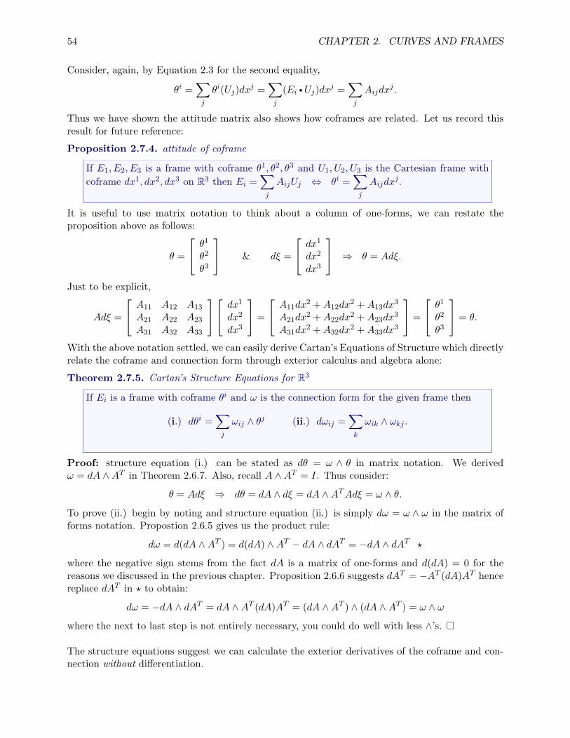
54 CHAPTER 2. CURVES AND FRAMES
Consider, again, by Equation 2.3 for the second equality,
θi =∑j
θi(Uj)dxj =
∑j
(Ei •Uj)dxj =
∑j
Aijdxj .
Thus we have shown the attitude matrix also shows how coframes are related. Let us record thisresult for future reference:
Proposition 2.7.4. attitude of coframe
If E1, E2, E3 is a frame with coframe θ1, θ2, θ3 and U1, U2, U3 is the Cartesian frame with
coframe dx1, dx2, dx3 on R3 then Ei =∑j
AijUj ⇔ θi =∑j
Aijdxj .
It is useful to use matrix notation to think about a column of one-forms, we can restate theproposition above as follows:
θ =
θ1
θ2
θ3
& dξ =
dx1
dx2
dx3
⇒ θ = Adξ.
Just to be explicit,
Adξ =
A11 A12 A13
A21 A22 A23
A31 A32 A33
dx1
dx2
dx3
=
A11dx2 +A12dx
2 +A13dx3
A21dx2 +A22dx
2 +A23dx3
A31dx2 +A32dx
2 +A33dx3
=
θ1
θ2
θ3
= θ.
With the above notation settled, we can easily derive Cartan’s Equations of Structure which directlyrelate the coframe and connection form through exterior calculus and algebra alone:
Theorem 2.7.5. Cartan’s Structure Equations for R3
If Ei is a frame with coframe θi and ω is the connection form for the given frame then
(i.) dθi =∑j
ωij ∧ θj (ii.) dωij =∑k
ωik ∧ ωkj .
Proof: structure equation (i.) can be stated as dθ = ω ∧ θ in matrix notation. We derivedω = dA ∧AT in Theorem 2.6.7. Also, recall A ∧AT = I. Thus consider:
θ = Adξ ⇒ dθ = dA ∧ dξ = dA ∧ATAdξ = ω ∧ θ.
To prove (ii.) begin by noting and structure equation (ii.) is simply dω = ω ∧ ω in the matrix offorms notation. Propostion 2.6.5 gives us the product rule:
dω = d(dA ∧AT ) = d(dA) ∧AT − dA ∧ dAT = −dA ∧ dAT ?
where the negative sign stems from the fact dA is a matrix of one-forms and d(dA) = 0 for thereasons we discussed in the previous chapter. Proposition 2.6.6 suggests dAT = −AT (dA)AT hencereplace dAT in ? to obtain:
dω = −dA ∧ dAT = dA ∧AT (dA)AT = (dA ∧AT ) ∧ (dA ∧AT ) = ω ∧ ω
where the next to last step is not entirely necessary, you could do well with less ∧’s. �
The structure equations suggest we can calculate the exterior derivatives of the coframe and con-nection without differentiation.

2.7. COFRAMES AND THE STRUCTURE EQUATIONS OF CARTAN 55
Example 2.7.6. Following Examples 2.2.9, 2.2.15 and 2.6.8 consider for the cylindrical frame:
A =
cos θ sin θ 0− sin θ cos θ 0
0 0 1
& ω =
0 dθ 0−dθ 0 0
0 0 0
I can read from A that the coframe and frame are:
θ1 = cos θ dx+ sin θ dyθ2 = − sin θ dx+ cos θ dyθ3 = dz.
&E1 = cos θ U1 + sin θ U2 = ∂rE2 = − sin θ U1 + cos θ U2 = r∂θE3 = U3.
Note x = r cos θ and y = r sin θ imply dx = cos θ dr − r sin θdθ and dy = sin θ dr + r cos θdθ. Thus,
θ1 = cos θ [cos θ dr − r sin θdθ] + sin θ [sin θ dr + r cos θdθ] = dr.
This is good, θ1(E1) = dr(∂r) = 1. Likewise, we can derive θ2 = rdθ and θ3 = dz. Therefore,
ω ∧ θ =
0 dθ 0−dθ 0 0
0 0 0
∧ drrdθdz
=
−rdθ ∧ dθ−dθ ∧ dr0
Of course dθ ∧ dθ = 0 hence (ω ∧ θ)1 = (ω ∧ θ)3 = 0 and (ω ∧ θ)2 = dr ∧ dθ. Naturally,
dθ1 = dθ3 = 0 & dθ2 = d(rdθ) = dr ∧ dθ.
So, we have confirmed the first structure equation of Cartan.
Another use of the structure equations is to derive the connection form from the coframe in a subtlemanner. In the next example I begin with the coframe of the spherical coordinate system followingExamples 2.2.10, 2.2.16 and 2.6.9.
Example 2.7.7. The coframe to the spherical frame introduced in Example 2.2.10 is given by:
θ1 = dρ, θ2 = ρ dφ, θ3 = ρ sinφdθ
Take exterior derivatives:
dθ1 = 0,
dθ2 = dρ ∧ dφ,dθ3 = sinφdρ ∧ dθ + ρ cosφdφ ∧ dθ.
Hence, the first structure equations yield:
(I.) dθ1 = ω12 ∧ θ2 + ω13 ∧ θ3 = ω12 ∧ (ρ dφ) + ω13 ∧ (ρ sinφdθ) = 0
(II.) dθ2 = −ω12 ∧ θ1 + ω23 ∧ θ3 = −ω12 ∧ dρ+ ω23 ∧ (ρ sinφdθ) = dρ ∧ dφ,(III.) dθ3 = −ω13 ∧ θ1 − ω23 ∧ θ2 = −ω13 ∧ dρ− ω23 ∧ (ρ dφ) = sinφdρ ∧ dθ + ρ cosφdφ ∧ dθ.
We can see from these equations that:
ω12 = dφ, ω13 = sinφdθ, ω23 = cosφdθ ⇒ ω =
0 dφ sinφdθ−dφ 0 cosφdθ
− sinφdθ − cosφdθ 0
If you compare with Example 2.6.9 then you can see we agree.

56 CHAPTER 2. CURVES AND FRAMES
Chapter 3
euclidean geometry
The study of euclidean geometry is greatly simplified by the use of analytic geometry. In particular,R3 provides a model in which the axioms of Euclid are easily realized for lines and points. The ex-change of axioms for equations and linear algebra is not a fair trade. Certainly the modern studenthas a great advantage over those ancients who had mere compass and straightedge constructivegeometry. Since the time of Descartes we have identified euclidean geometry with the study ofpoints in R2 or R3. We continue this tradition of analytic geometry in this chapter.
Given we take Rn as euclidean space, we begin by defining the distance between points in termsof the norm and dot product in Rn. We study special functions called isometries which preservethe distance between points. We show translations and rotations maintain the distance betweenpoints. Reflections also are seen to be isometries. It happens that these examples are exhaustive.We are able to prove that any isometry which fixes 0 must be an orthgonal transformation. Note,orthogonal transformations are linear transformations which makes them espcially nice. Then, witha bit more effort, we show that an abitrary isometry is simply a composite of a translation andorthogonal transformation which is sometimes called a rigid motion.
With points settled, we move on to vectors. We see that the push forwards of isometries are or-thogonal transformations on tangent vectors. We note the velocity α′ is naturally transformedby the push forward for any smooth function, but, for an isometry we get derivatives α′′, α′′′, . . .preserved under the push forward. For an arbitrary smooth function the higher derivatives wouldnot transform so simply, but, we don’t investigate that further here1. The generality of this sectionis not really needed for following O’neill, but, I take a couple pages to share the theory of Frenetcurves as given in Kuhnel. This natural extension to n-dimensions brings us to study curvaturesκ1, . . . , κn−2, κn−1 where the last curvature serves as the torsion. The Frenet Serret equations inRn are very similar and we sketch solutions for the constant curvature case.
In the last section we return to work on explicit results for frames and curves in the exclusivelythree dimensional case. We show a pair of frames at distinct points can be connected by a uniqueisometry. Moreover, the formula for this isometry is simply formulated in terms of the attitudesof the frames involved. We also show the push forward preserves the dot and cross product. Thisallows us to show the Frenet frame, curvature and torsion are nearly preserved by the push forwardof an isometry. The one caveat, the sign of the torsion can be reversed if the isometry is formed byan isometry which has an orthogonal transformation which is not a pure rotation. We conclude by
1see page 116 of O’neill for an example
57

58 CHAPTER 3. EUCLIDEAN GEOMETRY
defining congruence and we prove that two arclength parametrized curves are congruent if andonly if they share the same curvature and torsion functions.
3.1 isometries of euclidean space
We are primarily interested in three dimensional space, but, as it requires little extra effort andit actually simplifies some proofs we adopt an n-dimensional view. We use the euclidean distancefunction d(p, q) = ||q − p|| where ||v|| =
√v • v in what follows:
Definition 3.1.1. isometry in Rn:
We say F : Rn → Rn is an isometry of Rn when d(F (p), F (q)) = d(p, q) for all p, q ∈ Rn.
In other words, an isometry of Rn is a function on Rn which preserves distances. The set of allisometries naturally forms a group2 with respect to the composition of functions.
Proposition 3.1.2. composition of isometries is an isometry:
If F,G are isometries of Rn then F ◦G is an isometry is an isometry of Rn.
Proof: suppose F,G : Rn → Rn such that d(F (p), F (q)) = d(p, q) and d(G(p), G(q)) = d(p, q) forall p, q ∈ Rn then notice G(p), G(q) ∈ Rn hence:
d((F ◦G)(p), (F ◦G)(q)) = d((F (G(p)), F (G(q))) = d(G(p), G(q)) = d(p, q).
for all p, q ∈ Rn. Thus F ◦G is an isometry of Rn �
There are three examples of isometries which should be familar to the reader:
Example 3.1.3. T is a translation if there exists a ∈ Rn for which T (x) = x+ a for all x ∈ Rn.
d(T (p), T (q)) = ||T (q)− T (p)|| = ||(q + a)− (p+ a)|| = ||q − p|| = d(p, q).
It is also interesting to note the group theoretic properties of the set of all translations on Rn.Suppose we denote3 the set of all translations by T then if T, S ∈ T then T ◦S ∈ T and ifT (x) = x+a then T−1(x) = x−a and we see T−1 ∈ T . Finally, Id(x) = x+ 0 thus identify Id ∈ Tand we see T forms a group with respect to composition of functions. The action of translationson Rn is transitive. In particular, if p, q ∈ Rn then there exists T ∈ T for which T (p) = q. To seethis is true just observe T (x) = x+ a with a = q − p has T (p) = q and clearly T ∈ T .
Example 3.1.4. R is a orthogonal transformation if R is a linear transformation for which[R]T [R] = I where [R] denotes the standard matrix of R : Rn → Rn. A typical example in R3 isgiven by the rotation about the z-axis:
[R] =
cos θ sin θ 0− sin θ cos θ 0
0 0 1
.which has det([R]) = 1 or the reflection S(x) = −x which has det([S]) = −1.
2the proof of closure under inverse and existence of identity are implicitly covered later in this section.3I actually am unaware of any standard notation
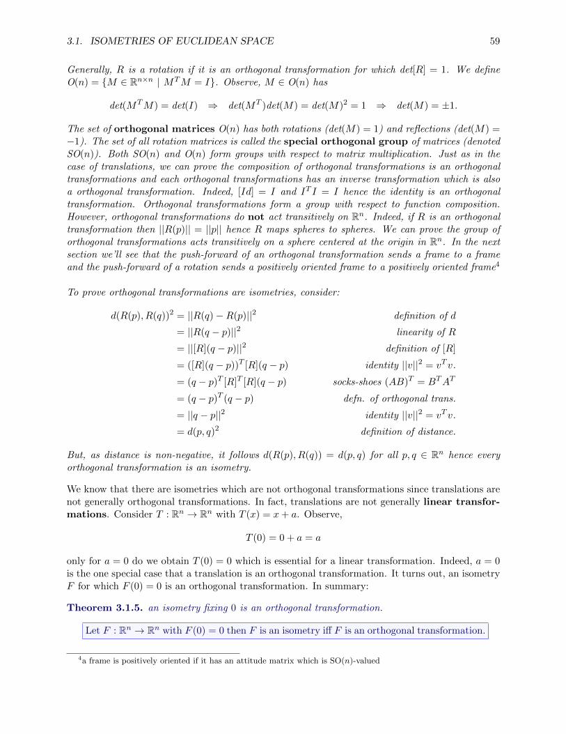
3.1. ISOMETRIES OF EUCLIDEAN SPACE 59
Generally, R is a rotation if it is an orthogonal transformation for which det[R] = 1. We defineO(n) = {M ∈ Rn×n | MTM = I}. Observe, M ∈ O(n) has
det(MTM) = det(I) ⇒ det(MT )det(M) = det(M)2 = 1 ⇒ det(M) = ±1.
The set of orthogonal matrices O(n) has both rotations (det(M) = 1) and reflections (det(M) =−1). The set of all rotation matrices is called the special orthogonal group of matrices (denotedSO(n)). Both SO(n) and O(n) form groups with respect to matrix multiplication. Just as in thecase of translations, we can prove the composition of orthogonal transformations is an orthogonaltransformations and each orthogonal transformations has an inverse transformation which is alsoa orthogonal transformation. Indeed, [Id] = I and IT I = I hence the identity is an orthogonaltransformation. Orthogonal transformations form a group with respect to function composition.However, orthogonal transformations do not act transitively on Rn. Indeed, if R is an orthogonaltransformation then ||R(p)|| = ||p|| hence R maps spheres to spheres. We can prove the group oforthogonal transformations acts transitively on a sphere centered at the origin in Rn. In the nextsection we’ll see that the push-forward of an orthogonal transformation sends a frame to a frameand the push-forward of a rotation sends a positively oriented frame to a positively oriented frame4
To prove orthogonal transformations are isometries, consider:
d(R(p), R(q))2 = ||R(q)−R(p)||2 definition of d
= ||R(q − p)||2 linearity of R
= ||[R](q − p)||2 definition of [R]
= ([R](q − p))T [R](q − p) identity ||v||2 = vT v.
= (q − p)T [R]T [R](q − p) socks-shoes (AB)T = BTAT
= (q − p)T (q − p) defn. of orthogonal trans.
= ||q − p||2 identity ||v||2 = vT v.
= d(p, q)2 definition of distance.
But, as distance is non-negative, it follows d(R(p), R(q)) = d(p, q) for all p, q ∈ Rn hence everyorthogonal transformation is an isometry.
We know that there are isometries which are not orthogonal transformations since translations arenot generally orthogonal transformations. In fact, translations are not generally linear transfor-mations. Consider T : Rn → Rn with T (x) = x+ a. Observe,
T (0) = 0 + a = a
only for a = 0 do we obtain T (0) = 0 which is essential for a linear transformation. Indeed, a = 0is the one special case that a translation is an orthogonal transformation. It turns out, an isometryF for which F (0) = 0 is an orthogonal transformation. In summary:
Theorem 3.1.5. an isometry fixing 0 is an orthogonal transformation.
Let F : Rn → Rn with F (0) = 0 then F is an isometry iff F is an orthogonal transformation.
4a frame is positively oriented if it has an attitude matrix which is SO(n)-valued

60 CHAPTER 3. EUCLIDEAN GEOMETRY
Proof: the converse direction of the theorem was already shown in Example 3.1.4 as, by definition,orthogonal transformation F is linear hence F (0) = 0.
Let us suppose F is an isometry for which F (0) = 0. Notice d(F (p), F (0)) = d(p, 0) impliesd(F (p), 0) = d(p, 0) which gives ||F (p)|| = ||p|| for all p ∈ Rn. Since ||F (p)|| = ||p|| it follows p 6= 0implies F (p) 6= 0. Therefore, F is not identically zero. Furthermore, we can show the image of Fincludes an orthogonal set of n nontrivial vectors. Consider the standard basis of Rn, (ei)
j = δij .Observe F (ei) •F (ej) = ei • ej = δij . Thus {F (e1), F (e2), . . . , F (en)} is an orthogonal basis for Rn.
Let p, q ∈ Rn and note:
d(F (p), F (q))2 = ||F (q)− F (p)||2
= (F (q)− F (p)) • (F (q)− F (p))
= F (q) •F (q)− 2F (p) •F (q) + F (p) •F (p)
= ||F (q)||2 − 2F (p) •F (q) + ||F (p)||2 ?
likewise,d(p, q)2 = ||q − p||2 = ||q||2 − 2p • q + ||p||2 ?2 .
Therefore, as d(F (p), F (q)) = d(p, q), we compare ? and ?2 and use ||F (p)|| = ||p|| and ||F (q)|| =||q|| to derive F (p) •F (q) = p • q for all p, q ∈ Rn. We seek to show F is a linear transformation:suppose x, y, z ∈ Rn and c ∈ R,
F (cx+ y) •F (z) = (cx+ y) • z = cx • z + y • z = cF (x) •F (z) + F (y) •F (z)
thusF (cx+ y) •F (z)− cF (x) •F (z)− F (y) •F (z) = 0.
By algebra of the dot product,[F (cx+ y)− cF (x)− F (y)
]•F (z) = 0.
But, if we take z = ei for i = 1, 2, . . . , n then the equation above shows the vector F (cx + y) −cF (x)− F (y) is zero in the F (ei)-direction for i = 1, 2, . . . , n hence F (cx+ y)− cF (x)− F (y) = 0.Therefore, F (cx+ y) = cF (x) + F (y) for all x, y ∈ Rn and c ∈ R. Finally, as F is linear, the linearalgebra gives a matrix R for which F (x) = Rx for all x ∈ Rn and it follows
yT Iz = y • z = F (y) •F (z) = (Ry) • (Rz) = yTRTRz
hence RTR = I and we conclude F is an orthogonal transformation. �
If we drop the requirement that F (0) = 0 for an isometry then the possibilities are still quitelimited. It turns out that every isometry of Rn is simply a composition of a translation and anorthogonal transformation.
Theorem 3.1.6. an isometries are generated by translations and orthgonal transformations
Every isometry F : Rn → Rn can be written uniquely as F = T ◦R where T is a translationand R is an orthogonal transformation. That is, there exists M ∈ O(n) and a ∈ Rn suchthat F (x) = Mx+ a for each x ∈ Rn.
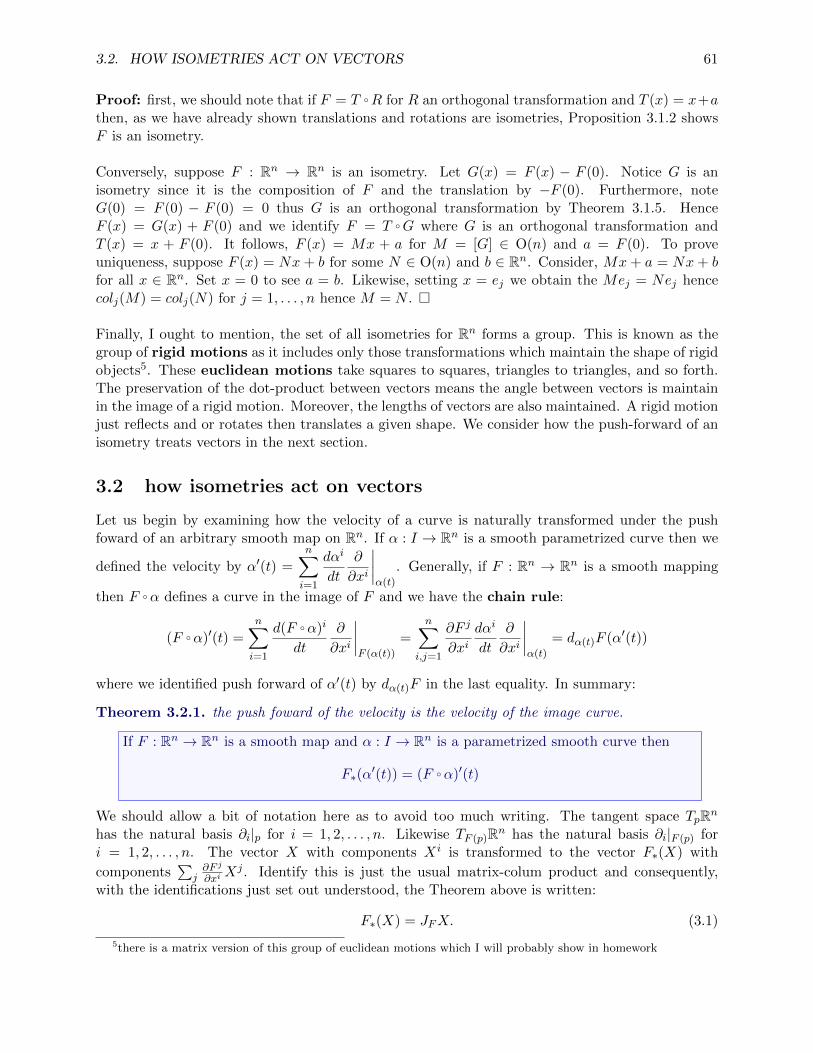
3.2. HOW ISOMETRIES ACT ON VECTORS 61
Proof: first, we should note that if F = T ◦R for R an orthogonal transformation and T (x) = x+athen, as we have already shown translations and rotations are isometries, Proposition 3.1.2 showsF is an isometry.
Conversely, suppose F : Rn → Rn is an isometry. Let G(x) = F (x) − F (0). Notice G is anisometry since it is the composition of F and the translation by −F (0). Furthermore, noteG(0) = F (0) − F (0) = 0 thus G is an orthogonal transformation by Theorem 3.1.5. HenceF (x) = G(x) + F (0) and we identify F = T ◦G where G is an orthogonal transformation andT (x) = x + F (0). It follows, F (x) = Mx + a for M = [G] ∈ O(n) and a = F (0). To proveuniqueness, suppose F (x) = Nx+ b for some N ∈ O(n) and b ∈ Rn. Consider, Mx+ a = Nx+ bfor all x ∈ Rn. Set x = 0 to see a = b. Likewise, setting x = ej we obtain the Mej = Nej hencecolj(M) = colj(N) for j = 1, . . . , n hence M = N . �
Finally, I ought to mention, the set of all isometries for Rn forms a group. This is known as thegroup of rigid motions as it includes only those transformations which maintain the shape of rigidobjects5. These euclidean motions take squares to squares, triangles to triangles, and so forth.The preservation of the dot-product between vectors means the angle between vectors is maintainin the image of a rigid motion. Moreover, the lengths of vectors are also maintained. A rigid motionjust reflects and or rotates then translates a given shape. We consider how the push-forward of anisometry treats vectors in the next section.
3.2 how isometries act on vectors
Let us begin by examining how the velocity of a curve is naturally transformed under the pushfoward of an arbitrary smooth map on Rn. If α : I → Rn is a smooth parametrized curve then we
defined the velocity by α′(t) =n∑i=1
dαi
dt
∂
∂xi
∣∣∣∣α(t)
. Generally, if F : Rn → Rn is a smooth mapping
then F ◦α defines a curve in the image of F and we have the chain rule:
(F ◦α)′(t) =
n∑i=1
d(F ◦α)i
dt
∂
∂xi
∣∣∣∣F (α(t))
=
n∑i,j=1
∂F j
∂xidαi
dt
∂
∂xi
∣∣∣∣α(t)
= dα(t)F (α′(t))
where we identified push forward of α′(t) by dα(t)F in the last equality. In summary:
Theorem 3.2.1. the push foward of the velocity is the velocity of the image curve.
If F : Rn → Rn is a smooth map and α : I → Rn is a parametrized smooth curve then
F∗(α′(t)) = (F ◦α)′(t)
We should allow a bit of notation here as to avoid too much writing. The tangent space TpRnhas the natural basis ∂i|p for i = 1, 2, . . . , n. Likewise TF (p)Rn has the natural basis ∂i|F (p) fori = 1, 2, . . . , n. The vector X with components Xi is transformed to the vector F∗(X) with
components∑
j∂F j
∂xiXj . Identify this is just the usual matrix-colum product and consequently,
with the identifications just set out understood, the Theorem above is written:
F∗(X) = JFX. (3.1)
5there is a matrix version of this group of euclidean motions which I will probably show in homework
62 CHAPTER 3. EUCLIDEAN GEOMETRY
Where (JF )ij = ∂F j
∂xiin the usual linear algebra index notation.
If F is an isometry of Rn then F (x) = Rx+ a for all x ∈ Rn for some R ∈ O(n) and a ∈ Rn. Note,
F i(x) =n∑j=1
Rijxj + ai ⇒ ∂F i
∂xk=
n∑j=1
∂
∂xk[Rijx
j]
+∂
∂xk[ai]
=n∑j=1
Rij∂xj
∂xk= Rij .
The calculation above shows the Jacobian matrix of an isometry is simply the orthogonal matrixfor the orthogonal transformation of the isometry. Thus, in view of Equation 3.1 we find:
F∗(v) = Rv (3.2)
where to be more carefull, F∗(p, v) = (F (p), Rv). Let me cease this ritual of notation and say some-thing interesting: Theorem 3.2.1 applied to an isometry gives us the result that the push forwardof a k-jet6 is the k-jet of the image curve under the isometry.
Recall we defined α′′ for a parametrized curve in R3. We define the k-th derivative of α in Rn inthe same fashion:
α(k)(t) =
n∑i=1
dkαi
dtk∂
∂xi
∣∣∣∣α(t)
=
(α(t),
⟨dkα1
dtk, . . . ,
dkαn
dtk
⟩).
Thus, α′′ = (α′)′ and generally α(k) = (α(k−1))′ for k ∈ N where we use Defn. 2.3.3 to differentiatethe velocity vector fields of velocity, acceleration and so forth along α.
Theorem 3.2.2. natural transfer of k-jet by isometry of Rn.
Suppose an isometry F : Rn → Rn is written as F (x) = Rx+ a for a ∈ Rn and R ∈ O(n).Also, suppose α : I → Rn is a smooth parametrized curve. Then: for k ∈ N,
F∗(α′) = (F ◦α)′, F∗(α
′′) = (F ◦α)′′, . . . , F∗(α(k)) = (F ◦α)(k).
Moreover, the magnitude of α(i) angle between α(i) and α(j) is preserved under F∗.
||F∗(α(i)(t))|| = ||α(i)(t)|| & F∗(α(i)(t)) •F∗(α
(j)(t)) = α(i)(t) •α(j)(t)
for each t ∈ I and i, j = 1, 2, . . . , n.
Proof: in Definition 2.3.6 Use Equation 3.2 and set v = α(k)(t)
F∗(α(k)(t)) = Rα(k)(t)
for k ∈ N. On the other hand the image curve F ◦α has:
(F ◦α)(t) = Rα(t) + a ⇒ (F ◦α)(k)(t) = Rα(k)(t) = F∗(α(k)(t)).
Omitting the t-dependence,
F∗(α(k)) = Rα(k)
6see page 12 of Kuhnel for a related concept of the k-th order contact of two curves. The k-jet of a curve can beidentified with an equivalence class of curves whose initial k derivatives align at the given point

3.2. HOW ISOMETRIES ACT ON VECTORS 63
Hence angles between derivatives and their magnitudes of α are preserved under the push-forwardof an isometry since orthogonal matrices preserve the dot product and hence the norm and angles. �
Specialize to n = 3 for a moment. Given a nonlinear regular curve α we defined T,N,B along α.Moreover, T,N,B are all derived from dot and cross products of α′ and α′′ hence the curvatureand torsion of α and F ◦α will match perfectly provided we preserve the cross-product7. It turnsout that forces us to require the isometry has det(R) = 1.
We should also pause to consider the significance of Theorem 3.2.2 to Newtonian Mechanics. Thecentral equation of mechanics is Fnet = ma. Of course, this equation is made with respect toa particular coordinate system. If we change to another coordinate system which is related tothe first by an isometry then the acceleration naturally transforms. Of course, the story is a bitmore complicated since the coordinate systems in physics also can move. We could think about theT,N,B frame moving with the curve. Indeed, many of the annoyning gifs on my webpage are basedon this idea. But, the isometries we’ve studied in this chapter have no time dependence. That said,allowing the coordinate systems to move just introduces an additional constant velocity motionin addition to the isometries we primarily study here. If you’d like to read a somewhat formaltreatment of Newtonian Mechanics then you might enjoy Chapter 6 of my notes from Math 430which I taught as a graduate student at NCSU. I describe something called a Euclidean Structurewhich gives a natural mathematical setting to describe the concept of an observer and a movingframe of reference. Then in Chapter 7 of those notes I describe a Minkowski Structure which doesthe same for Special Relativity8. I don’t think I’ll cover it, but I should mention Kuhnel treatscurves in Minkowski space and the low-dimensional geometry of curves and surfaces in manifoldswith Lorentzian geometry is still quite active.
3.2.1 Frenet curves in Rn
Let me pause from our general development to introduce the theory of Frenet curves from Chapter2 of Wolfgang Kuhnel’s Differential Geometry : Curves-Surfaces-Manifolds. Here we find a gener-alization of the T,N,B construction for n-dimensional space and the results we have proved thusfar for push fowards of isometries will go to prove that a Frenet curve and its isometric image haveall same curvatures and the same torsion if the isometry is comprised of a rotation and translation.
Definition 3.2.3. frame in Rn:
If E1, . . . , En ∈ X(Rn) are orthonormal vector fields then we say {E1, . . . , En} is a frameof Rn. If Ei =
∑j AijEj then A is the attitude matrix of the frame. Frames for which
det(A) = 1 are called positively oriented frames and frames with det(A) = −1 are saidto be negatively oriented.
In Rn we use determinant to play the role the cross-product played in R3. If we have n − 1orthonormal vectors E1, . . . , En−1 then the vector En =
∑j(En)jUj will be defined by
(En)j = det [E1| . . . |En−1|Uj ] . (3.3)
In the construction of the Frenet frame described below the first (n − 1) vectors in the frame aregenerated by the Gram-Schmidt algorithm applied the linearly independent derivatives and higher
7I think this is quite plausible, but we will prove it later, see Theorem 3.3.48I should be clear, these notes closely parallel a presentation of Math 430 I enjoyed as an undergraduate from
R.O. Fulp and certainly the main mathematical ideas are his and the mistakes are most likely mine.
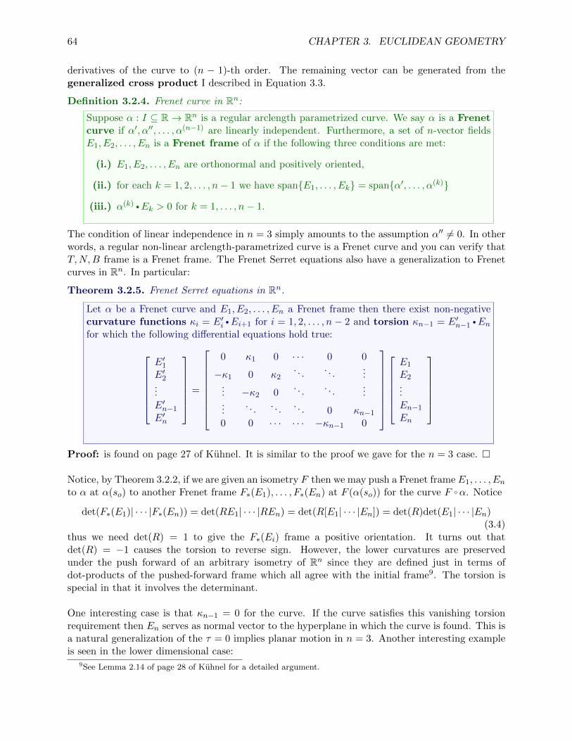
64 CHAPTER 3. EUCLIDEAN GEOMETRY
derivatives of the curve to (n − 1)-th order. The remaining vector can be generated from thegeneralized cross product I described in Equation 3.3.
Definition 3.2.4. Frenet curve in Rn:
Suppose α : I ⊆ R→ Rn is a regular arclength parametrized curve. We say α is a Frenetcurve if α′, α′′, . . . , α(n−1) are linearly independent. Furthermore, a set of n-vector fieldsE1, E2, . . . , En is a Frenet frame of α if the following three conditions are met:
(i.) E1, E2, . . . , En are orthonormal and positively oriented,
(ii.) for each k = 1, 2, . . . , n− 1 we have span{E1, . . . , Ek} = span{α′, . . . , α(k)}
(iii.) α(k) •Ek > 0 for k = 1, . . . , n− 1.
The condition of linear independence in n = 3 simply amounts to the assumption α′′ 6= 0. In otherwords, a regular non-linear arclength-parametrized curve is a Frenet curve and you can verify thatT,N,B frame is a Frenet frame. The Frenet Serret equations also have a generalization to Frenetcurves in Rn. In particular:
Theorem 3.2.5. Frenet Serret equations in Rn.
Let α be a Frenet curve and E1, E2, . . . , En a Frenet frame then there exist non-negativecurvature functions κi = E′i •Ei+1 for i = 1, 2, . . . , n− 2 and torsion κn−1 = E′n−1
•Enfor which the following differential equations hold true:
E′1E′2...E′n−1
E′n
=
0 κ1 0 · · · 0 0
−κ1 0 κ2. . .
. . ....
... −κ2 0. . .
. . ....
.... . .
. . .. . . 0 κn−1
0 0 · · · · · · −κn−1 0
E1
E2...En−1
En
Proof: is found on page 27 of Kuhnel. It is similar to the proof we gave for the n = 3 case. �
Notice, by Theorem 3.2.2, if we are given an isometry F then we may push a Frenet frame E1, . . . , Ento α at α(so) to another Frenet frame F∗(E1), . . . , F∗(En) at F (α(so)) for the curve F ◦α. Notice
det(F∗(E1)| · · · |F∗(En)) = det(RE1| · · · |REn) = det(R[E1| · · · |En]) = det(R)det(E1| · · · |En)(3.4)
thus we need det(R) = 1 to give the F∗(Ei) frame a positive orientation. It turns out thatdet(R) = −1 causes the torsion to reverse sign. However, the lower curvatures are preservedunder the push forward of an arbitrary isometry of Rn since they are defined just in terms ofdot-products of the pushed-forward frame which all agree with the initial frame9. The torsion isspecial in that it involves the determinant.
One interesting case is that κn−1 = 0 for the curve. If the curve satisfies this vanishing torsionrequirement then En serves as normal vector to the hyperplane in which the curve is found. This isa natural generalization of the τ = 0 implies planar motion in n = 3. Another interesting exampleis seen in the lower dimensional case:
9See Lemma 2.14 of page 28 of Kuhnel for a detailed argument.

3.2. HOW ISOMETRIES ACT ON VECTORS 65
Example 3.2.6. Suppose we have a Frenet curve in R2. It suffices to have a regular curve; that isα : I → R2 with α′(s) 6= 0 for all s ∈ I. If E1, E2 is defined by:
E1(s) = α′(s) = a(s)U1 + b(s)U2 & E2(s) = −b(s)U1 + a(s)U2
where the unit-speed assumption means the functions a, b must satisfy a2 + b2 = 1. We definecurvature κ = ||E′1|| which gives:
κ =√
(a′)2 + (b′)2
For example, α(s) = (R cos(s/R), R sin(s/R)) gives α′(s) = − sin(s/R)U1 + cos(s/R)U2 = E1 thus
E′1 = − cos(s/R)R U1 − sin(s/R)
R U2 ⇒ κ = 1R .
The reverse question is also very interesting. In particular, given a set of curvature functions and atorsion function when can we find a Frenet curve which takes the given functions as its curvatureand torsion?
Theorem 3.2.7. on solving Frenet Serret equations in Rn.
Suppose we are given (n − 1) smooth functions κi : (a, b) → R for which κi(s) ≥ 0 fors ∈ (a, b) and i = 1, 2, . . . , n− 2. Also, suppose a point qo and a frame v1, . . . vn ∈ TqoRn isgiven. Let so ∈ (a, b). There exists a unique Frenet curve α for which α(s0) = qo and thecurve has Frenet frame E1, . . . , En for which Ei(so) = vi for i = 1, . . . , n and κi = E′i •Ei+1
for i = 1, . . . , n− 1.
Proof: a slightly improved version of the above theorem as well as the proof is found on page 28of of Kuhnel. Ultimately this theorem, like so many others, rests on the existence and uniquenesstheorem for solutions of systems of ordinary differential equations. �
We found in Example 3.2.6 that a circle has constant curvature which is reciprocal to its radius.The example which follows investigates the reverse question:
Example 3.2.8. Find the arclength parametrized curve in R2 for which κ(s) = 1/R for all s. Weseek to solve:
E′1 = κE2, E′2 = −κE1
Differentiate the first equation and subsitute the second equation to obtain:
E′′1 = −κ2E1
This gives10 E1 = cos(κs)C1 +sin(κs)C2 for constant vectors C1, C2. Next, by E2 = 1κE′1 we derive:
E2 = − sin(κs)C1 + cos(κs)C2
Finally, the curve itself is found from integrating α′(s) = E1(s):
α(s) = αo +1
κsin(κs)C1 −
1
κcos(κs)C2.
Of course, the constant vectors C1, C2 must be specified such that ||E1|| = 1 and ||E2|| = 1. Observe,
||α(s)− αo|| =1
κ|| sin(κs)C1 − cos(κs)C2|| =
1
κ|| − E2|| = R.
Just as we hoped, this is a circle of radius R = 1/κ centered at αo.
10in terms of the usual ODEs course, think of E1 = yU1 + zU2 thus E′′1 + κ2E1 = 0 yields y′′ + κ2y = 0 andz′′ + κ2z = 0. Then the usual techniques yield y = C11 cosκs + C12 sinκs and z = C21 cosκs + C22 sinκs hencecombining those we obtain my claimed vector solution with C1 = (C11, C12) and C2 = (C21, C22)
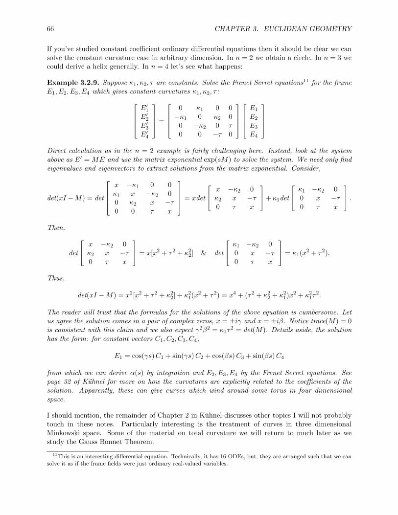
66 CHAPTER 3. EUCLIDEAN GEOMETRY
If you’ve studied constant coefficient ordinary differential equations then it should be clear we cansolve the constant curvature case in arbitrary dimension. In n = 2 we obtain a circle. In n = 3 wecould derive a helix generally. In n = 4 let’s see what happens:
Example 3.2.9. Suppose κ1, κ2, τ are constants. Solve the Frenet Serret equations11 for the frameE1, E2, E3, E4 which gives constant curvatures κ1, κ2, τ :
E′1E′2E′3E′4
=
0 κ1 0 0−κ1 0 κ2 0
0 −κ2 0 τ0 0 −τ 0
E1
E2
E3
E4
Direct calculation as in the n = 2 example is fairly challenging here. Instead, look at the systemabove as E′ = ME and use the matrix exponential exp(sM) to solve the system. We need only findeigenvalues and eigenvectors to extract solutions from the matrix exponential. Consider,
det(xI −M) = det
x −κ1 0 0κ1 x −κ2 00 κ2 x −τ0 0 τ x
= xdet
x −κ2 0κ2 x −τ0 τ x
+ κ1det
κ1 −κ2 00 x −τ0 τ x
.Then,
det
x −κ2 0κ2 x −τ0 τ x
= x[x2 + τ2 + κ22] & det
κ1 −κ2 00 x −τ0 τ x
= κ1(x2 + τ2).
Thus,
det(xI −M) = x2[x2 + τ2 + κ22] + κ2
1(x2 + τ2) = x4 + (τ2 + κ22 + κ2
1)x2 + κ21τ
2.
The reader will trust that the formulas for the solutions of the above equation is cumbersome. Letus agree the solution comes in a pair of complex zeros, x = ±iγ and x = ±iβ. Notice trace(M) = 0is consistent with this claim and we also expect γ2β2 = κ1τ
2 = det(M). Details aside, the solutionhas the form: for constant vectors C1, C2, C3, C4,
E1 = cos(γs)C1 + sin(γs)C2 + cos(βs)C3 + sin(βs)C4
from which we can derive α(s) by integration and E2, E3, E4 by the Frenet Serret equations. Seepage 32 of Kuhnel for more on how the curvatures are explicitly related to the coefficients of thesolution. Apparently, these can give curves which wind around some torus in four dimensionalspace.
I should mention, the remainder of Chapter 2 in Kuhnel discusses other topics I will not probablytouch in these notes. Particularly interesting is the treatment of curves in three dimensionalMinkowski space. Some of the material on total curvature we will return to much later as westudy the Gauss Bonnet Theorem.
11This is an interesting differential equation. Technically, it has 16 ODEs, but, they are arranged such that we cansolve it as if the frame fields were just ordinary real-valued variables.

3.3. ON FRAMES AND CONGRUENCE IN THREE DIMENSIONS 67
3.3 on frames and congruence in three dimensions
Much of what is done in this section for Rn, but, I resist the temptation and simply work in R3.
We saw after Example 3.1.3 that translations act transitively on R3. Something similar is true forisometries and frames in R3; suppose we have a pair of frames E1, E2, E3 and F1, F2, F3 at p. Wecan find an orthogonal transformation Φ which transfers E to F . We seek Φ for which
Φ∗(E1) = F1, Φ∗(E2) = F2, Φ∗(E3) = F3.
If the matrix of Φ∗ is R then
R[E1] = [F1], R[E2] = [F2], R[E3] = [F3]
where Ei = Ai1U1 + Ai2U2 + Ai3U3 for i = 1, 2, 3 implies [Ei] = [Ai1, Ai2, Ai3]T . Likewise, Fi =Bi1U1 +Bi2U2 +Bi3U3. Concatenate the three equations above into a single equation to obtain:
RAT = BT ⇒ R = BTA.
Since the attitude matrices A,B exist for a given pair of frames at p it follows that Φ(x) = BTAxdefines the desired isometry which pushes the E-frame to the F -frame. With this calculation inhand, the theorem below is easy to prove:
Theorem 3.3.1. transfer of frame by isometry.
Let E1, E2, E3 ∈ TpR3 be a frame at p with attitude A and F1, F2, F3 ∈ TqR3 be a frame atq with attitude B then there exists an isometry Φ : R3 → R3 for which Φ(p) = q and
Φ∗(E1) = F1, Φ∗(E2) = F2, Φ∗(E3) = F3.
Proof: let R = BTA and define Φ(x) = Rx+q−Rp for all x ∈ R3. Observe Φ(p) = Rp+q−Rp = qas desired. Furthermore, as ATA = I we find R = BTA implies RAT = BT . But, this shows thematrix R maps each row of A to the corresponding row of B. Hence the push-forward with matrixR maps vectors with coordinates formed by rows of A to new vectors with coordinates formed byrows of B. But, Ei has coordinates in [rowi(A)]T and Fi has coordinates in [rowi(B)]T thus
Φ∗(Ei) = Fi
where Ei is at p and Fi is at Φ(p) = q. �
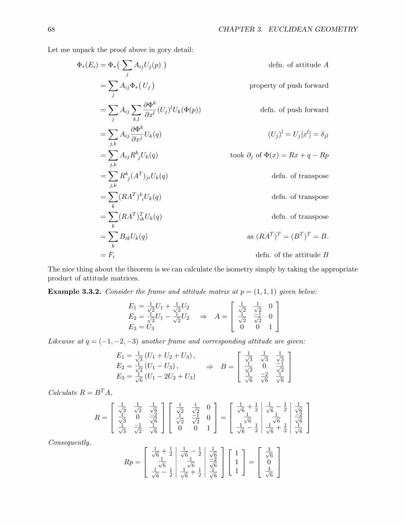
68 CHAPTER 3. EUCLIDEAN GEOMETRY
Let me unpack the proof above in gory detail:
Φ∗(Ei) = Φ∗( ∑
j
AijUj(p))
defn. of attitude A
=∑j
AijΦ∗(Uj)
property of push forward
=∑j
Aij∑k,l
∂Φk
∂xl(Uj)
lUk(Φ(p)) defn. of push forward
=∑j,k
Aij∂Φk
∂xjUk(q) (Uj)
l = Uj [xl] = δjl
=∑j,k
AijRkjUk(q) took ∂j of Φ(x) = Rx+ q −Rp
=∑j,k
Rkj(AT )jiUk(q) defn. of transpose
=∑k
(RAT )kiUk(q) defn. of transpose
=∑k
(RAT )TikUk(q) defn. of transpose
=∑k
BikUk(q) as (RAT )T = (BT )T = B.
= Fi defn. of the attitude B
The nice thing about the theorem is we can calculate the isometry simply by taking the appropriateproduct of attitude matrices.
Example 3.3.2. Consider the frame and attitude matrix at p = (1, 1, 1) given below:
E1 = 1√2U1 + 1√
2U2
E2 = 1√2U1 − 1√
2U2
E3 = U3
⇒ A =
1√2
1√2
01√2−1√
20
0 0 1
Likewise at q = (−1,−2,−3) another frame and corresponding attitude are given:
E1 = 1√3
(U1 + U2 + U3) ,
E2 = 1√2
(U1 − U3) ,
E3 = 1√6
(U1 − 2U2 + U3)
⇒ B =
1√3
1√3
1√3
1√2
0 −1√2
1√6−2√
61√6
Calculate R = BTA,
R =
1√3
1√2
1√6
1√3
0 −2√6
1√3−1√
21√6
1√2
1√2
01√2−1√
20
0 0 1
=
1√6
+ 12
1√6− 1
21√6
1√6
1√6
−2√6
1√6− 1
21√6
+ 12
1√6
Consequently,
Rp =
1√6
+ 12
1√6− 1
21√6
1√6
1√6
−2√6
1√6− 1
21√6
+ 12
1√6
1
11
=
3√6
03√6
3.3. ON FRAMES AND CONGRUENCE IN THREE DIMENSIONS 69
Thus, using Φ(x) = Rx+ q −Rp we have:
Φ(x, y, z) =
1√6
+ 12
1√6− 1
21√6
1√6
1√6
−2√6
1√6− 1
21√6
+ 12
1√6
xyz
− 1 + 3√
6
23 + 3√
6
.I invite the reader to verify that Φ∗ pushes the E-frame to the F -frame as claimed. It is easy tocheck that the product of the transpose of i-th row of A with R yields the transpose of the i-th rowof B hence Φ∗(Ei) = Fi for i = 1, 2, 3.
Let us return to the discussion we initiated with Equation 3.4.
Theorem 3.3.3. isometries and push forward of vector products in R3
Suppose F : R3 → R3 is an isometry and V,W ∈ X(R3) then
F∗(V ) •F∗(W ) = V •W & F∗(V )× F∗(W ) = det(F∗)F∗(V ×W ).
Proof: following12 Equation 3.2 suppose the orthogonal matrix for F is R,
F∗(V ) •F∗(W ) = (RV ) • (RW )
= (RV )T (RW )
= V TRTRW = V TW = V •W.
Likewise,F∗(V )× F∗(W ) = (RV )× (RW )
Notice, RTR = I and F∗(U1), F∗(U2), F∗(U3) forms a frame thus as F∗(Uj) = RUj ,
(F∗(V )× F∗(W )) •Uj = ((RV )× (RW )) •Uj = det[RV |RW |Uj
]Note RTR = I allows
[RV |RW |RRTUj
]= R
[V |W |RTUj
]hence
det[RV |RW |Uj
]= det(R)det
[V |W |RTUj
]and as det(F∗) = det(R) we find
(F∗(V )× F∗(W )) •Uj = det(F∗)det[V |W |RTUj
]= det(F∗)(V ×W ) •RTUj
Thus, as (V ×W ) •RTUj = R(V ×W ) •Uj = F∗(V ×W ) •Uj for each j = 1, 2, 3 we derive:
F∗(V )× F∗(W ) = det(F∗)F∗(V ×W ). �
The proof given above equally well applies to vector fields along some curve. You may recall fromTheorem 3.2.2 we already know dot product is preserved between vector fields α′, α′′, . . . along αwhen pushed forward to the curve F ◦α where F is an isometry. Also, notice det(F∗) = R forcesdet(F∗) = ±1 since RTR = I implies det(R) = ±1. It follows that only the isometries built fromrotations (det(R) = 1) preserve the full Frenet apparatus for a non-linear regular curve.
12the matrix products below are products of the coordinate vectors with respect to U1, U2, U3
70 CHAPTER 3. EUCLIDEAN GEOMETRY
Theorem 3.3.4. Frenet apparatus of curve’s isometric image
Let α be a nonlinear arclength parametrized regular curve with Frenet frame T,N,B andcurvature κ and torsion τ . Suppose F : R3 → R3 is an isometry and define α = F ◦α.If T ,N,B and κ and τ form the Frenet apparatus for α then
T = F∗(T ), N = F∗(N), B = det(F∗)F∗(B), κ = κ, τ = det(F∗)τ.
Proof: the unit tangents for α and α are defined as T (s) = α′(s) and T (s) = α′(s) = (F ◦α)′(s).In Theorem 3.2.2 we learned F∗(α
′) = (F ◦α)′ thus T (s) = F∗(T ).
The Frenet normal for α and α are defined by N(s) = 1κα′′ and N(s) = 1
κ α′′ where κ = ||α′′||
and κ = ||α′′||. However, as α′′ = (F ◦α)′′ and Theorem 3.2.2 provides F∗(α′′) = (F ◦α)′′ and
||F∗(α′′)|| = ||α′′|| thus ||α′′|| = ||(F ◦α)′′|| = ||α′′|| we derive κ = κ and:
F∗(N) = F∗
(1
||α′′||α′′)
=1
||α′′||F∗(α
′′) =1
||(F ◦α)′′||(F ◦α)′′ = N.
The binormal of α and α are defined as B = T ×N and B = T ×N . Therefore, by Theorem 3.3.3,
F∗(B) = F∗(T ×N) = det(F∗)F∗(T )× F∗(N) = det(F∗)T ×N = det(F∗)B.
The torsions of α and α are defined by τ = −B′ •N and τ = −B′ •N . Apply Theorem 3.3.3,
B′ •N = F∗(B′) •F∗(N)
I invite the reader to prove the small lemma F∗(B′) = det(F∗)B
′from which we find:
B′ •N = F∗(B′) •F∗(N) = det(F∗)B
′•N
Therefore, τ = det(F∗)τ . �
The theorem above shows we can maintain the curvature and torsion of a curve when we transformthe curve by rotation and translation.
Example 3.3.5. Suppose α(s) = (R cos(s/√R2 +m2), R sin(s/
√R2 +m2),ms/
√R2 +m2). Let
θ = s/√R2 +m2. Consider F (x, y, z) = (y, x, z). This is a simple isometry which has det(F∗) =
−1. Considerα(s) = (F ◦α)(s) = (R sin(θ), R cos(θ),mθ)
then we calculate,
T =1√
R2 +m2[R cos θ U1 −R sin θ U2 +mU3] & N = − sin θ U1 − cos θ U2
Thus, B = T ×N yields
B =1√
R2 +m2[m cos θ U1 −m sin θ U2 −RU3]
Differentiate, note θ′ = 1/√R2 +m2 hence by chain rule:
B′=
1
R2 +m2[−m sin θ U1 −m cos θ U2] ⇒ τ = −B′ •N =
−mm2 +R2
.

3.3. ON FRAMES AND CONGRUENCE IN THREE DIMENSIONS 71
Notice that the torsion of α is the negative of that which we found in Example 2.4.4. The helixα follows a left-hand-rule whereas the original helix α winds in a right-handed fashion. Swappingsine and cosine amounts to changing from a clockwise to a counter-clockwise winding as viewedfrom the positive z-axis. If you consider the T ×N verses T ×N geometrically it is easy to see Bpoints up whereas B points down relative to the positive z-axis. But, both α and α have a positivez-velocity hence the curve bends up off the osculating plane in the α case but, it bends down off theosculating plane in the α case.
Following O’neill, we define two curves to be congruent if they have the same speed and shape.This is concisely given by:
Definition 3.3.6. congruence of parametrized curves
We say two parametrized curves α : I → R3 and β : I → R3 are congruent if there existsan isometry F for which β = F ◦α.
Since isometries generally have rather complicated formulas this allows us to twist given standardexamples into nearly unrecognizable forms:
Example 3.3.7. Consider the parametrized curve:
β(t) =(c1R cos t+ c2R sin t+ c3mt− 1 + 3/
√6,
c3R cos t+ c3R sin t− 2c3mt− 2,
c2R cos t+ c1R sin t+ c3mt− 3− 3/√
6)
where c1 = 1/√
6 + 1/2, c2 = 1/√
6− 1/2 and c3 = 1/√
6. In fact, this is just the helix with radiusR and slope m. To see this simply x = R cos t, y = R sin t and z = mt into the isometry
F (x, y, z) =
1√6
+ 12
1√6− 1
21√6
1√6
1√6
−2√6
1√6− 1
21√6
+ 12
1√6
xyz
− 1 + 3√
6
23 + 3√
6
.as to obtain β(t) by calculating F (α(t)).
You can see identifying standard curves simply by their formulas is generally a formidable task.
Definition 3.3.8. parallel curves
We say two parametrized curves α : I → R3 and β : I → R3 are parallel if there existsp ∈ R3 for which β(t) = α(t) + p for all t ∈ I.
Part (i.) of Theorem 2.3.8 told us γ′(t) = 0 for all t ∈ I iff γ(t) = p for all t ∈ I. If we studyγ(t) = β(t)− α(t) then the proposition below follows naturally from Theorem 2.3.8.
Proposition 3.3.9.
Parametrized curves α, β : I → R3 are parallel if and only if α′(t) = β′(t) for all t ∈ I.Moreover, if α and β are parallel and there exists to for which α(to) = β(to) then α = β.
Proof: suppose α, β : I → R3 are parallel hence β(t) = α(t) + p for all t ∈ I. Differentiate to
see β′(t) = α′(t) for all t ∈ I. Conversely, suppose β′(t) = α′(t) for all t ∈ I. Thus dαi
dt = dβi
dt fori = 1, 2, 3. Integrate with respect to t to obtain αi(t) = βi(t) + pi for i = 1, 2, 3 where pi ∈ R is
72 CHAPTER 3. EUCLIDEAN GEOMETRY
a constant. Thus, α(t) = β(t) + p for each t ∈ I. Finally, suppose α, β : I → R3 are parallel withα(to) = β(to). But, β(t) = α(t) + p also implies β(to) = α(to) + p hence α(to) = α(to) + p thusp = 0 and we conclude β = α. �
This definition of parallel covers more than just lines. The usual theorems for parallel lines ineuclidean space clearly do not apply:
Example 3.3.10. If α(t) = (R cos t, R sin t, 0) and β(t) = (a + R cos t, b + R sin t, c) then β(t) =α(t) + (a, b, c). These are parallel circles. If c = 0 and a, b are sufficiently small, these parallelcircles can be distinct and yet intersect.
Finally we come to the central result of this Chapter. Equivalence of curvature and torsion providesequivalence of curves. Here we think of two arclength parametrized curves as equivalent if theyare congruent. You can show that congruence is an equivalence relation. So, another way tounderstand the theorem which follows is that the curvature and torsion functions serve as labelsfor the equivalence class of unit-speed curves related by rigid motions.
Theorem 3.3.11. curves classified by curvature and torsion in R3
Arclength parametrized curves α, α : I → R3 are congruent iff κ = κ and τ = ±τ .
Proof: Theorem 3.3.4 shows congruent curves have the same curvature and torsion modulo a sign.It remains to prove the converse direction. Suppose α, α : I → R3 are arclength parametrizedcurves for which κ = κ and τ = ±τ . Suppose so ∈ I and τ = τ define F to be the unique isometrywhich pushes the Frenet frame of α at α(so) to the Frenet frame of α at α(so):
T o = F∗(To), No = F∗(No), Bo = F∗(Bo), F (α(so)) = α(so) ? (so)
where To = T (so) etc. Notice, I only claim initially that F∗ matches the Frenet frames at s = so. Weknow this is possible by Theorem 3.3.1. Apply Theorem 3.3.4 to show F∗(T ), F∗(N), F∗(B) solvethe Frenet Serret equations with κ and τ coefficients. Therefore, we have Frenet Serret equationsfor the F ◦α Frenet frame and the α Frenet frame: let me set κ = κ and τ = τ for our futurecalculational convenience:
F∗(T )′ = κF∗(N)F∗(N)′ = −κF∗(T ) + τ F∗(B)F∗(B)′ = −τF∗(N)
&
T′= κN
N′= −κT + τ B
B′= −τN
(3.5)
We wish to show F ◦α = α. Notice, as (F ◦α)′ = F∗(T ) and α′ = T to show F ◦α and α areparallel we must show F∗(T ) and T have the same vector parts. But, this is nicely captured by thedot-product F∗(T ) •T = 1 since both ||F∗(T )|| = ||T || = 1. Moreover, we know F∗(T (so)) = T (so)by construction of F hence we simply need to show that the function g(s) = F∗(T (s)) •T (s) hasconstant value of 1. It turns out that is not directly successful, so, we instead follow O’neill13 andinvolve the entire Frenet frames. Set
f(s) = F∗(T (s)) •T (s) + F∗(N(s)) •N(s) + F∗(B(s)) •B(s)
Omit the s-dependence and differentiate:
f ′ = F∗(T )′ •T + F∗(T ) •T′+ F∗(N)′ •N + F∗(N) •N
′+ F∗(B)′ •B + F∗(B) •B
′
13beware, my α is his β on page 122-123

3.3. ON FRAMES AND CONGRUENCE IN THREE DIMENSIONS 73
Subtitute Equation 3.5 to obtain:
f ′ =κF∗(N) •T + F∗(T ) •κN +(−κF∗(T ) + τ F∗(B)
)•N
+ F∗(N) •(−κT + τ B
)+−τF∗(N) •B + F∗(B) •
(−τN
)= 0
But, f(so) = F∗(T (so)) •T (so) + F∗(N(so)) •N(so) + F∗(B(so)) •B(so) = 3 thus all three dot-products must be identically 1 and we find that F ◦α and α are parallel with (F ◦α)(so) = α(so)thus, by Proposition 3.3.9, we conclude F ◦α = α. Hence α and α are congruent in the case τ = τ .I leave the τ = −τ case to the reader. �
This theorem easily generalizes to the case of non-unit speed. The derivation just includes a fewextra speed factors. The Proposition below exhibits the power of the theorem towards questions ofclassification:
Proposition 3.3.12.
If α be an arclength parametrized curve then α has constant κ, τ iff α is a helix.
Proof: In Example 2.4.4 we introduced the standard helix defined by R,m > 0 and
α(s) = (R cos(ks), R sin(ks),mks)
for s ∈ R and k = 1/√R2 +m2. We calculated:
κ =R
R2 +m2& τ =
m
R2 +m2
If F is an isometry then F ◦α is also a helix and by Theorem 3.3.4 the non-standard helix alsohas κ = R
R2+m2 and τ = ±mR2+m2 . Conversely, suppose α is an arclength parametrized curve with
constant κ and τ . Observe, if we set values for R and m as
R =κ
κ2 + τ2, & m =
τ
κ2 + τ2
then
R
R2 +m2=
κκ2+τ2
κ2
(κ2+τ2)2+ τ2
(κ2+τ2)2
= κ &m
R2 +m2=
τκ2+τ2
κ2
(κ2+τ2)2+ τ2
(κ2+τ2)2
= τ.
Hence, by Theorem 3.3.11 the curve α with constant κ and τ is congruent to the helix withR = κ
κ2+τ2and m = τ
κ2+τ2since the helix and α have the same curvature and torsion. �
Also, the reader may enjoy Example 5.4 on page 124 of O’neill which explicitly shows how a pair ofhelices with opposite-signed torsion are connected by an isometry with an orthogonal matrix withdeterminant −1.
The result below is needed for Theorem 9.2 on page 316-317 of O’neill where this result is criticalto prove something about the isometry of surfaces. The proof is placed here since the technique isvery much reminiscent of proof given for Theorem 3.3.11. Notice, the frames in the theorem beloware not assumed to be Frenet frames. The assignment of the frame along the curve could be madeby some other set of rules.
74 CHAPTER 3. EUCLIDEAN GEOMETRY
Theorem 3.3.13. curve congruence for arbitrary frames
Suppose α, β : I → R3 are parametrized curves. Also, let E1, E2, E3 be a frame field alongα and F1, F2, F3 a frame field along β. If the two conditions below hold true then α and βare congruent. For 1 ≤ i, j ≤ 3,
(1.) α′ •Ei = β′ •Fi & (2.) E′i •Ej = F ′i •Fj .
In particular, in the case these conditions are met, the isometry G for which β = G ◦α isdefined by any to ∈ I where we construct G∗(Ei(α(to))) = Fi(β(to)) for i = 1, 2, 3.
Proof: see page 126 of O’neill. �