Lecture Notes #9 - Curvesmycsvtunotes.weebly.com/.../computer_graphics_unit2.pdf• For Graphics,...

COS 426 Lecture Notes #9

Lecture Notes #9 - Curves

Reading:

Angel: Chapter 9

Foley et al., Sections 11(intro) and 11.2

Overview

Introduction to mathematical splines

Bezier curves

Continuity conditions (C0, C1, C2, G1, G2)

Creating continuous splines

C2 interpolating splines

B-splines

Catmull-Rom splines

1


Introduction

2

Mathematical splines are motivated by the "loftsman's spline":

• Long, narrow strip of wood or plastic

• Used to fit curves through specified data points

• Shaped by lead weights called "ducks"

• Gives curves that are "smooth" or "fair"

Such splines have been used for designing:

• Automobiles

• Ship hulls

• Aircraft fuselages and wings


Requirements

3

Here are some requirements we might like to have in our mathematical splines:

• Predictable control

• Multiple values

• Local control

• Versatility

• Continuity


Mathematical splines

4

The mathematical splines we'll use are:

• Piecewise

• Parametric

• Polynomials

Let's look at each of these terms......


Parametric curves

5

In general, a "parametric" curve in the plane is expressed as:

x = x(t)

y = y(t)

Example: A circle with radius r centered at the origin is given by:

x = r cos t

y = r sin t

By contrast, an "implicit" representation of the circle is:


Parametric polynomial curves

6

A parametric "polynomial" curve is a parametric curve where each function x(t), y(t) is described by a polynomial:

Polynomial curves have certain advantages:

• Easy to compute

• Infinitely differentiable

Σ aiti

i=0

nx(t) =

Σ biti

i=0

ny(t) =


Piecewise parametric polynomial curves

7

A "piecewise" parametric polynomial curve uses different polynomial functions for different parts of the curve.

• Advantage: Provides flexibility

• Problem: How do you guarantee smoothness at the joints? (Problem known as "continuity.")

In the rest of this lecture, we'll look at:

1. Bezier curves -- general class of polynomial curves

2. Splines -- ways of putting these curves together


Bezier curves

8

• Developed simultaneously by Bezier (at Renault) and deCasteljau (at Citroen), circa 1960.

• The Bezier curve Q(u) is defined by nested interpolation:

• Vi's are "control points"

• { V0, ... , Vn} is the "control polygon"


Bezier curves: Basic properties

9

Bezier curves enjoy some nice properties:

• Endpoint interpolation:

• Convex hull: The curve is contained in the convex hull of its control polygon

• Symmetry:

Q(0) = V0

Q(1) = Vn

Q(u) defined by {V0, ..., Vn}

Q(1 - u) defined by {Vn, ... , V0}


Bezier curves: Explicit formulation

10

Let's give Vi a superscript V

ij to indicate the level of nesting.

An explicit formulation for Q(u) is given by the recurrence:

Vij = (1 - u) V

ij-1 + uV

i+1j-1


Explicit formulation, cont.

11

For n = 2, we have:

Q(u) = V02

= (1 - u)V01 + uV1

1

= (1 - u) [(1 - u) V00 + uV1

0] + [(1 - u) V10 + uV2

0]

= (1 - u)2V00 + 2u(1 - u)V1

0 + u2V20

In general:

Bin(u) is the i'th Bernstein polynomial of degree n.

Q(u) = Vin

i

i= 0

n

∑ ui (1− u)n− i

Bin(u)


Bezier curves: More properties

12

Here are some more properties of Bezier curves

Q(u) = Vin

i

i= 0

n

∑ ui (1− u)n− i

• Degree: Q(u) is a polynomial of degree n

• Control points: How many conditions must we specify to uniquely determine a Bezier curve of degree n?


More properties, cont.

13

• Tangents:

Q'(0) = n(V1 - V0)

Q'(1) = n(Vn - V

n-1)

• k'th derivatives: In general,

• Q(k)(0) depends only on V0, ..., Vk

• Q(k)(1) depends only on Vn, ..., V

n-k

• (At intermediate points u (0, 1), all control points are involved for every derivative.)


Cubic curves

14

For the rest of this discussion, we'll restrict ourselves to piecewise cubic curves.

• In CAGD, higher-order curves are often used

• Gives more freedom in design

• Can provide higher degree of continuity between pieces

• For Graphics, piecewise cubic let's you do just about anything

• Lowest degree for specifiying points to interpolate and tangents

• Lowest degree for specifying curve in space

All the ideas here generalize to higher-order curves


Matrix form of Bezier curves

15

Bezier curves can also be described in matrix form:

3Q(u) = Vi

3

i

i= 0∑ ui (1− u)3− i

= (1 - u)3 V0 + 3u (1 - u)2 V1 + 3u2 (1 - u) V2 + u3 V3

-1 3 -3 1 3 -6 3 0-3 3 0 0 1 0 0 0

= u3 u2 u 1

V0

V1

V2

V3

= u3 u2 u 1

V0

V1

V2

V3

MBezier


Display: Recursive subdivision

16

Q: Suppose you wanted to draw one of these Bezier curves -- how would you do it?

A: Recursive subdivision:


Display, cont.

17

Here's pseudocode for the recursive subdivision display algorithm:

procedure Display({ V0, ..., Vn}):

if {V0, ..., Vn} flat within ε then

Output line segment V0Vn

else

Subdivide to produce {L0, ..., Ln} and {R0, ..., Rn

}

Display({ L0, ..., Ln})

Display({ R0, ..., Rn})

end if

end procedure


Splines

18

To build up more complex curves, we can piece together different Bezier curves to make "splines."

For example, we can get:

• Positional (C0) continuity:

• Derivative (C1) continuity:

Q: How would you build an interactive system to satisfy these constraints?


Advantages of splines

19

Advantages of splines over higher-order Bezier curves:

• Numerically more stable

• Easier to compute

• Fewer bumps and wiggles


Tangent (G1) continuity

20

Q: Suppose the tangents were in opposite directions but not of same magnitude -- how does the curve appear?

This construction gives "tangent (G1) continuity."

Q: How is G1 continuity different from C1?


Curvature (C2) continuity

21

Q: Suppose you want even higher degrees of continuity -- e.g., not just slopes but curvatures -- what additional geometric constraints are imposed?

We'll begin by developing some more mathematics.....


Operator calculus

22

Let's use a tool known as "operator calculus."

Define the operator D by:

DVi V

i+1

Rewriting our explicit formulation in this notation gives:

Q(u) = Vin

i

i = 0

n∑ ui (1− u)n− i

= Din

i

i = 0

n∑ ui (1− u)n− i

= V0n

i

i = 0

n∑ (uD)i (1− u)n− i

V0

Applying the binomial theorem gives: = (uD + (1 - u))n V0


Taking the derivative

23

One advantage of this form is that now we can take the derivative:

Q'(u) = n(uD + (1 - u))n-1 (D - 1) V0

What's (D - 1) V0?

Plugging in and expanding:

This gives us a general expression for the derivative Q'(u).

= Din - 1

i

i= 0

n-1∑ ui (1− u)n−1 - i (V0n V1)Q'(u)


Specializing to n = 3

24

What's the derivative Q'(u) for a cubic Bezier curve?

Note that:

• When u = 0: Q'(u) = 3(V1 - V0)

• When u = 1: Q'(u) = 3(V3 - V2)

Geometric interpretation:

So for C1 continuity, we need to set:

3(V3 - V2) = 3(W1 - W0)


Taking the second derivative

25

Taking the derivative once again yields:

Q''(u) = n (n - 1) (uD + (1 - u))n-2 (D - 1)2 V0

What does (D - 1)2 do?


Second-order continuity

26

So the conditions for second-order continuity are:

(V3 - V2) = (W1 - W0)

(V3 - V2) - (V2 - V1) = (W2 - W1) - (W1 - W0)

Putting these together gives:

Geometric interpretation


C3 continuity

27

Summary of continuity conditions

• C0 straightforward, but generally not enough• C3 is too constrained (with cubics)


Creating continuous splines

28

We'll look at three ways to specify splines with C1 and C2 continuity:

1. C2 interpolating splines

2. B-splines

3. Catmull-Rom splines


C2 Interpolating splines

29

The control points specified by the user, called "joints," are interpolated by the spline.

For each of x and y, we needed to specify ______ conditions for each cubic Bezier segment.

So if there are m segments, we'll need ______ constraints.

Q: How many of these constraints are determined by each joint?


In-depth analysis, cont.

30

At each interior joint j, we have:

1. Last curve ends at j

2. Next curve begins at j

3. Tangents of two curves at j are equal

4. Curvature of two curves at j are equal

The m segments give:

• ______ interior joints

• ______ conditions

The 2 end joints give 2 further contraints:

1. First curve begins at first joint

2. Last curve ends at last joint

Gives _______ constraints altogether.


End conditions

31

The analysis shows that specifying m + 1 joints for m segments leaves 2 extra degrees of freedom.

These 2 extra constraints can be specified in a variety of ways:

• An interactive system

• Constraints specified as ________

• "Natural" cubic splines

• Second derivatives at endpoints defined to be 0

• Maximal continuity

• Require C3 continuity between first and last pairs of curves


C2 Interpolating splines

32

Problem: Describe an interactive system for specifiying C2 interpolating splines.

Solution:

1. Let user specify first four Bezier control points.

2. This constrains next _____ control points -- draw these in.

3. User then picks _____ more

4. Repeat steps 2-3.


Global vs. local control

33

These C2 interpolating splines yield only "global control" -- moving any one joint (or control point) changes the entire curve!

Global control is problematic:

• Makes splines difficult to design

• Makes incremental display inefficient

There's a fix, but nothing comes for free. Two choices:

• B-splines

• Keep C2 continuity

• Give up interpolation

• Catmull-Rom splines

• Keep interpolation

• Give up C2 continuity -- provides C1 only


B-splines

34

Previous construction (C2 interpolating splines):

• Choose joints, constrained by the "A-frames."

New construction (B-splines):

• Choose points on A-frames

• Let these determine the rest of Bezier control points and joints

The B-splines I'll describe are known more precisely as "uniform B-splines."


B-spline construction

35

The points specified by the user in this construction are called "de Boor points."


B-spline properties

36

Here are some properties of B-splines:

• C2 continuity

• Approximating

• Does not interpolate deBoor points

• Locality

• Each segment determined by 4 deBoor points

• Each deBoor point determines 4 segments

• Convex hull

• Curve lies inside convex hull of deBoor points


Algebraic construction of B-splines

37

V1 = ______ B1 + ______ B2

V2 = ______ B1 + ______ B2

V0 = ______ [______ B0 + ______ B1] + ______ [______ B1 + ______ B2]

= ______ B0 + ______ B1 + ______ B2

V3 = ______ B1 + ______ B2 + ______ B3


Algebraic construction of B-splines, cont.

38

Once again, this construction can be expressed in terms of a matrix:

1 4 1 00 4 2 00 2 4 00 1 4 1

=

B0

B1

B2

B3

1

6

V0

V1

V2

V3


Drawing B-splines

39

Drawing B-splines is therefore quite simple:

procedure Draw-B-Spline ({B0, ..., Bn}):

for i = 0 to n - 3 do

Convert Bi, ..., B

i+3 into a Bezier control polygon V0, ..., V3

Display ({V0, ... , V3})

end for

end procedure


Multiple vertices

40

Q: What happens if you put more than one control point in the same place?

Some possibilities:

• Triple vertex

• Double vertex

• Collinear vertices


End conditions

41

You can also use multiple vertices at the endpoints:

• Double endpoint

• Curve tangent to line between first distinct points

• Triple endpoint

• Curve interpolates endpoint

• Starts out with a line segment

• Phantom vertices

• Gives interpolation without line segment at ends


Catmull-Rom splines

42

The Catmull-Rom splines

• Give up C2 continuity

• Keep interpolation

For the derivation, let's go back to the interpolation algorithm. We had 4 conditions at each joint j:

1. Last curve ends at j

2. Next curve begins at j

3. Tangents of two curves at j are equal

4. Curvature of two curves at j are equal

If we ...

• Eliminate condition 4

• Make condition 3 depend only on local control points

... then we can have local control!


Derivation of Catmull-Rom splines

43

Idea: (Same as B-splines)

• Start with joints to interpolate

• Build a cubic Bezier curve between successive points

The endpoints of the cubic Bezier are obvious:

V0 = B1

V3 = B2

Q: What should we do for the other two points?


Derivation of Catmull-Rom, cont.

44

A: Catmull & Rom use half the magnitude of the vector between adjacent control points:

Many other choices work -- for example, using an arbitrary constant τ times this vector gives a "tension" control.


Matrix formulation

45

The Catmull-Rom splines also admit a matrix formulation:

0 6 0 0-1 6 1 00 1 6 -10 0 6 0

=

B0

B1

B2

B3

1

6

V0

V1

V2

V3

Exercise: Derive this matrix.


Properties

46

Here are some properties of Catmull-Rom splines:

• C1 Continuity

• Interpolating

• Locality

• No convex hull property

• (Proof left as an exercise.)

(Spline, Bezier, B-Spline)

[email protected]

Spline

• Drafting terminology

– Spline is a flexible strip that is easily flexed to

pass through a series of design points (control

points) to produce a smooth curve.

• Spline curve – a piecewise polynomial

(cubic) curve whose first and second

derivatives are continuous across the

various curve sections.

2 [email protected]

Bezier curve

• Developed by Paul de Casteljau (1959) and

independently by Pierre Bezier (1962).

• French automobil company – Citroen &

Renault.

P0

P1 P2

P3

3 [email protected]

Parametric function

• P(u) = Bn,i(u)pi

Where

Bn,i(u) = . n!. ui(1-u)n-i

i!(n-i)! 0<= u<= 1

i=0

n

For 3 control points, n = 2

P(u) = (1-u)2p0 + 2u(1-u) p1+ u2p2

For four control points, n = 3

P(u) = (1-u)3p0 + 3u(1-u) 2 p1 + 3u 2 (1-u)p2 + u3p3

4 [email protected]

algorithm

• De Casteljau

– Basic concept

• To choose a point C in line segment AB such that C

divides the line segment AB in a ratio of u: 1-u

A B C

P0

P1

P2

Let u = 0.5

00 01 u=0.25

10

11

u=0.75

20

21

5 [email protected]

properties

• The curve passes through the first, P0 and last vertex points, Pn .

• The tangent vector at the starting point P0 must be given by P1 – P0 and the tangent Pn given by Pn – Pn-1

• This requirement is generalized for higher derivatives at the curve’s end points. E.g 2nd derivative at P0 can be determined by P0 ,P1 ,P2 (to satisfy continuity)

• The same curve is generated when the order of the control points is reversed 6 [email protected]

Properties (continued)

• Convex hull

– Convex polygon formed by connecting the

control points of the curve.

– Curve resides completely inside its convex hull

7 [email protected]

B-Spline

• Motivation (recall bezier curve)

– The degree of a Bezier Curve is determined by the number of control points

– E. g. (bezier curve degree 11) – difficult to bend the "neck" toward the line segment P4P5.

– Of course, we can add more control points.

– BUT this will increase the degree of the curve increase computational burden

8 [email protected]


– Joint many bezier curves of lower

degree together (right figure)

– BUT maintaining continuity in

the derivatives of the desired

order at the connection point is

not easy or may be tedious and

undesirable.

B-Spline

9 [email protected]

B-Spline


– moving a control point affects the

shape of the entire curve- (global

modification property) –

undesirable.

- Thus, the solution is B-Spline – the

degree of the curve is independent

of the number of control points

- E.g - right figure – a B-spline curve

of degree 3 defined by 8 control

points 10 [email protected]

• In fact, there are five Bézier curve segments of degree 3 joining together to form the B-spline curve defined by the control points

• little dots subdivide the B-spline curve into Bézier curve segments.

• Subdividing the curve directly is difficult to do so, subdivide the domain of the curve by points called knots

B-Spline

0 u 1

11 [email protected]

• In summary, to design a B-spline curve, we

need a set of control points, a set of knots

and a degree of curve.

B-Spline


• P(u) = Ni,k(u)pi (umin u umax).. (1.0)

Where basis function = Ni,k(u)

Degree of curve k-1

Control points, pi 0 i n

Knot, u umin u umax

max = n + k

2 k n+1

B-Spline curve

i=0

n


B-Spline : definition

• P(u) = Ni,k(u)pi (umin u um)

• ui knot

• [ui, ui+1) knot span

• (u0, u1, u2, …. um ) knot vector

• The point on the curve that corresponds to a knot ui, knot point ,P(ui)

• If knots are equally space uniform

• If knots are not equally space non uniform


• Uniform knot vector

– Individual knot value is evenly spaced

– (0, 1, 2, 3, 4)

– ( 0, 0.2, 0.4, 0.6…)

– Then, normalized to the range [0, 1]

– (0, 0.25, 0.5, 0.75, 1.0)

– (0.0,0.1,0.2,0.3,0.4,0.5,0.6,0.7,0.8,0.9,1.0)



• Non-Uniform knot vector

– Individual knot value is not evenly spaced

– (0, 1, 3, 7, 8)

– ( 0, 0.2, 0.3, 0.7……)

– (0, 0.1, 0.3, 0.4, 0.8 …)

– Then, normalized to the range [0, 1]

– (0, 0.15, 0.20, 0.35, 0.40,0.75,0.85,1.0)



Type of B-Spline uniform knot vector

Non-periodic knots

(open knots) Periodic knots

(non-open knots)

-First and last knots are

duplicated k times.

-E.g (0,0,0,1,2,2,2)

-Curve pass through the

first and last control

points

-First and last knots are

not duplicated – same

contribution.

-E.g (0, 1, 2, 3)

-Curve doesn’t pass

through end points.

- used to generate closed

curves (when first = last

control points) 17 [email protected]

Type of B-Spline Uniform knot

vector

Non-periodic knots

(open knots) Periodic knots

(non-open knots)

(Closed knots) 18 [email protected]

Non-periodic (open) uniform B-Spline

• The knot spacing is evenly spaced except at the ends

where knot values are repeated k times.

• E.g P(u) = Ni,k(u)pi (u0 u um)

• Degree = k-1, number of control points = n + 1

• Number of knots = m + 1 @ n+ k + 1

for degree = 1 and number of control points = 4 (k = 2, n = 3)

Number of knots = n + k + 1 = 6

Range = 0 to n+k

non periodic uniform knot vector (0,0,1,2,3, 3)

* Knot value between 0 and 3 are equally spaced

uniform

i=0

n


Questions

• For curve degree = 3, number of

control points = 5

• For curve degree = 1, number of

control points = 5

• k = ? , n = ? , Range = ?

Knot vector = ? 20 [email protected]

• Example

• For curve degree = 3, number of control points = 5

• k = 4, n = 4

• number of knots = n+k+1 = 9

• non periodic knots vector = (0,0,0,0,1,2,2,2,2)

• For curve degree = 1, number of control points = 5

• k = 2, n = 4

• number of knots = n + k + 1 = 7

• non periodic uniform knots vector = (0, 0, 1, 2, 3, 4, 4)



• For any value of parameters k and n, non

periodic knots are determined from


ui =

0 0 i < k

i – k + 1 k i n

n – k + 2 n < i n+k

e.g k=2, n = 3

ui =

0 0 i < 2

i – 2 + 1 2 i 3

3 – 2 + 2 3 < i 5

u = (0, 0, 1, 2, 3, 3)

(1.3)


B-Spline basis function

2 1

1,1

1

1,

,

iki

ki

ki

iki

ki

ikiuu

uNuu

uu

uNuuuN

3 selainnya. 0

1

1

1,

ii

i

uuuN

In equation (1.1), the denominators can have a value of

zero, 0/0 is presumed to be zero.

If the degree is zero basis function Ni,1(u) is 1 if u is in the

i-th knot span [ui, ui+1).

Otherwise

(1.1)

(1.2)


• For example, if we have four knots u0 = 0, u1 = 1, u2 = 2 and u3 = 3, knot spans 0, 1 and 2 are [0,1), [1,2), [2,3)

• the basis functions of degree 0 are N0,1(u) = 1 on [0,1) and 0 elsewhere, N1,1(u) = 1 on [1,2) and 0 elsewhere, and N2,1(u) = 1 on [2,3) and 0 elsewhere.

• This is shown below



• To understand the way of computing Ni,k(u) for k greater

than 0, we use the triangular computation scheme



Example

• Find the knot values of a non periodic

uniform B-Spline which has degree = 2 and

3 control points. Then, find the equation of

B-Spline curve in polynomial form.



Answer

• Degree = k-1 = 2 k=3

• Control points = n + 1 = 3 n=2

• Number of knot = n + k + 1 = 6

• Knot values 0,0,0,1,1,1



Answer(cont)

• To obtain the polynomial equation,

P(u) = Ni,k(u)pi

• = Ni,3(u)pi

• = N0,3(u)p0 + N1,3(u)p1 + N2,3(u)p2

• firstly, find the Ni,k(u) using the knot value that

shown above, start from k =1 to k=3


i=0

n

i=0

2


Answer (cont) • For k = 1, find Ni,1(u) – use equation (1.2):

• N0,1(u) = 1 u0 u u1 ; (u=0)

• 0 otherwise

• N1,1(u) = 1 u1 u u2 ; (u=0)

• 0 otherwise

• N2,1(u) = 1 u2 u u3 ; (0 u 1)

• 0 otherwise

• N3,1(u) = 1 u3 u u4 ; (u=1)

• 0 otherwise

• N4,1(u) = 1 u4 u u5 ; (u=1)

• 0 otherwise




• N0,2(u) = u - u0 N0,1 + u2 – u N1,1 (u0 =u1 =u2 = 0)

• u1 - u0 u2 – u1

• = u – 0 N0,1 + 0 – u N1,1 = 0

• 0 – 0 0 – 0

• N1,2(u) = u - u1 N1,1 + u3 – u N2,1 (u1 =u2 = 0, u3 = 1)

• u2 - u1 u3 – u2

• = u – 0 N1,1 + 1 – u N2,1 = 1 - u

• 0 – 0 1 – 0


2 1

1,1

1

1,

,

iki

ki

ki

iki

ki

ikiuu

uNuu

uu

uNuuuN


Answer (cont) • N2,2(u) = u – u2 N2,1 + u4 – u N3,1 (u2 =0, u3 =u4 = 1)

• u3 – u2 u4 – u3

• = u – 0 N2,1 + 1 – u N3,1 = u

• 1 – 0 1 – 1

• N3,2(u) = u – u3 N3,1 + u5 – u N4,1 (u3 =u4 = u5 = 1)

• u4 – u3 u5– u4

• = u – 1 N3,1 + 1 – u N4,1 = 0

• 1 – 1 1 – 1




Answer (cont) For k = 2

N0,2(u) = 0

N1,2(u) = 1 - u

N2,2(u) = u

N3,2(u) = 0



• N0,3(u) = u - u0 N0,2 + u3 – u N1,2 (u0 =u1 =u2 = 0, u3 =1 )

• u2 - u0 u3 – u1

• = u – 0 N0,2 + 1 – u N1,2 = (1-u)(1-u) = (1- u)2

• 0 – 0 1 – 0

• N1,3(u) = u - u1 N1,2 + u4 – u N2,2 (u1 =u2 = 0, u3 = u4 = 1)

• u3 - u1 u4 – u2

• = u – 0 N1,2 + 1 – u N2,2 = u(1 – u) +(1-u)u = 2u(1-u)

• 1 – 0 1 – 0


2 1

1,1

1

1,

,

iki

ki

ki

iki

ki

ikiuu

uNuu

uu

uNuuuN


Answer (cont) • N2,3(u) = u – u2 N2,2 + u5 – u N3,2 (u2 =0, u3 =u4 = u5 =1)

• u4 – u2 u5 – u3

• = u – 0 N2,2 + 1 – u N3,2 = u2

• 1 – 0 1 – 1

N0,3(u) =(1- u)2, N1,3(u) = 2u(1-u), N2,3(u) = u2

The polynomial equation, P(u) = Ni,k(u)pi • P(u) = N0,3(u)p0 + N1,3(u)p1 + N2,3(u)p2

• = (1- u)2 p0 + 2u(1-u) p1 + u2p2 (0 <= u <= 1)


i=0

n


• Exercise

• Find the polynomial equation for curve with

degree = 1 and number of control points = 4

Non-periodic (open) uniform B-

Spline


• Answer

• k = 2 , n = 3 number of knots = 6

• Knot vector = (0, 0, 1, 2, 3, 3) • For k = 1, find Ni,1(u) – use equation (1.2):

• N0,1(u) = 1 u0 u u1 ; (u=0)

• N1,1(u) = 1 u1 u u2 ; (0 u 1)

N2,1(u) = 1 u2 u u3 ; (1 u 2)

• N3,1(u) = 1 u3 u u4 ; (2 u 3)

N4,1(u) = 1 u4 u u5 ; (u=3)

•




• N0,2(u) = u - u0 N0,1 + u2 – u N1,1 (u0 =u1 =0, u2 = 1)

• u1 - u0 u2 – u1

• = u – 0 N0,1 + 1 – u N1,1

• 0 – 0 1 – 0

• = 1 – u (0 u 1)


2 1

1,1

1

1,

,

iki

ki

ki

iki

ki

ikiuu

uNuu

uu

uNuuuN



• N1,2(u) = u - u1 N1,1 + u3 – u N2,1 (u1 =0, u2 =1, u3 = 2)

• u2 - u1 u3 – u2

• = u – 0 N1,1 + 2 – u N2,1

• 1 – 0 2 – 1

• N1,2(u) = u (0 u 1)

• N1,2(u) = 2 – u (1 u 2)


2 1

1,1

1

1,

,

iki

ki

ki

iki

ki

ikiuu

uNuu

uu

uNuuuN


Answer (cont) • N2,2(u) = u – u2 N2,1 + u4 – u N3,1 (u2 =1, u3 =2,u4 = 3)

• u3 – u2 u4 – u3

• = u – 1 N2,1 + 3 – u N3,1 =

• 2 – 1 3 – 2

• N2,2(u) = u – 1 (1 u 2)

• N2,2(u) = 3 – u (2 u 3)



Answer (cont) • N3,2(u) = u – u3 N3,1 + u5 – u N4,1 (u3 = 2, u4 = 3, u5 = 3)

• u4 – u3 u5– u4

• = u – 2 N3,1 + 3 – u N4,1 =

• 3 – 2 3 – 3

• = u – 2 (2 u 3)



Answer (cont)

• The polynomial equation P(u) = Ni,k(u)pi • P(u) = N0,2(u)p0 + N1,2(u)p1 + N2,2(u)p2 + N3,2(u)p3

• P(u) = (1 – u) p0 + u p1 (0 u 1)

• P(u) = (2 – u) p1 + (u – 1) p2 (1 u 2)

• P(u) = (3 – u) p2 + (u - 2) p3 (2 u 3)



Periodic uniform knot

• Periodic knots are determined from

– Ui ; (0 i n+k)

• Example

– For curve with degree = 3 and number of control points = 4 (cubic B-spline)

– (k = 4, n = 3) number of knots = n+k+1 =8

– (0, 1, 2, 3, 4, 5, 6, 7)


• Normalize u (0<= u <= 1) • N0,4(u) = 1/6 (1-u)3

• N1,4(u) = 1/6 (3u 3 – 6u 2 +4)

• N2,4(u) = 1/6 (-3u 3 + 3u 2 + 3u +1)

• N3,4(u) = 1/6 u3

• P(u) = N0,4(u)p0 + N1,4(u)p1 + N2,4(u)p2 + N3,4(u)p3



• In matrix form

• P(u) = [u3,u2, u, 1].Mn.

• Mn = 1/6


P0

P1

P2

P3

-1 3 -3 1

3 -6 3 0

-3 0 3 0

1 4 1 0



P0


Closed periodic

P0

P1

P2

P3

P4

P5

Example

k = 4, n = 5


Equation 1.0 change to

• Ni,k(u) = N0,k((u-i)mod(n+1))

P(u) = N0,k((u-i)mod(n+1))pi

Closed periodic

i=0

n

0<= u <= n+1


48

Question 1

Construct the B-Spline curve of degree/order 3 with 4 polygon

vertices A(1,1), B(2,3), C(4,3) and D(6,2). Using Non-

Periodic Knot and Periodic Knot.

[email protected]

Properties of B-Spline

1. The m degree B-Spline function are

piecewise polynomials of degree m

have Cm-1 continuity. e.g B-Spline

degree 3 have C2 continuity.

u=1

u=2


Properties of B-Spline In general, the lower the degree, the closer a B-spline

curve follows its control polyline.

Degree = 7 Degree = 5 Degree = 3



Equality m = n + k must be satisfied

Number of knots = m + 1

k cannot exceed the number of control points, n+ 1



2. Each curve segment is affected by k control

points as shown by past examples. e.g k = 3,

P(u) = Ni-1,k pi-1 + Ni,k pi+ Ni+1,k pi+1



Local Modification Scheme: changing the position of control

point Pi only affects the curve C(u) on interval [ui, ui+k).

Modify control point P2


Properties of B-Spline 3. Strong Convex Hull Property: A B-spline curve is

contained in the convex hull of its control polyline.

More specifically, if u is in knot span [ui,ui+1), then C(u)

is in the convex hull of control points Pi-p, Pi-p+1, ..., Pi.

Degree = 3, k = 4

Convex hull based on 4

control points



4. Non-periodic B-spline curve C(u) passes through

the two end control points P0 and Pn.

5. Each B-spline function Nk,m(t) is nonnegative

for every t, and the family of such functions

sums to unity, that is Ni,k (u) = 1

6. Affine Invariance

to transform a B-Spline curve, we simply

transform each control points.

7. Bézier Curves Are Special Cases of B-spline

Curves

i=0

n


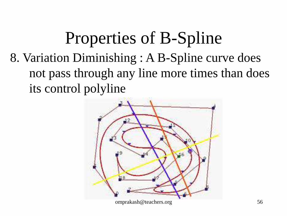
Properties of B-Spline 8. Variation Diminishing : A B-Spline curve does

not pass through any line more times than does

its control polyline


Knot Insertion : B-Spline

• knot insertion is adding a new knot into the existing knot vector without changing the shape of the curve.

• new knot may be equal to an existing knot the multiplicity of that knot is increased by one

• Since, number of knots = k + n + 1

• If the number of knots is increased by 1 either degree or number of control points must also be increased by 1.

• Maintain the curve shape maintain degree change the number of control points.


• So, inserting a new knot causes a new control point to be added. In fact, some existing control points are removed and replaced with new ones by corner cutting

Knot Insertion : B-Spline

Insert knot u = 0.5 58 [email protected]

Single knot insertion : B-Spline

• Given n+1 control points – P0, P1, .. Pn

• Knot vector, U= (u0, u1,…um)

• Degree = p, order, k = p+1

• Insert a new knot t into knot vector without

changing the shape.

• find the knot span that contains the new

knot. Let say [uk, uk+1)


Single knot insertion : B-Spline • This insertion will affected to k (degree + 1) control points

(refer to B-Spline properties) Pk, Pk-1, Pk-1,…Pk-p

• Find p new control points Qk on leg Pk-1Pk, Qk-1 on leg Pk-

2Pk-1, ..., and Qk-p+1 on leg Pk-pPk-p+1 such that the old

polyline between Pk-p and Pk (in black below) is replaced by

Pk-pQk-p+1...QkPk (in orange below)

Pk

Pk-1 Pk-2

Pk-p

Pk-p+1

Qk Qk-1

Qk-p+1 60 [email protected]


• All other control points are not change

• The formula for computing the new control

point Qi on leg Pi-1Pi is the following

• Qi = (1-ai)Pi-1+ aiPi

• ai = t- ui k-p+1<= i <= k

• ui+p-ui



• Example

• Suppose we have a B-spline curve of degree

3 with a knot vector as follows:

u0 to u3 u4 u5 u6 u7 u8 to u11

0 0.2 0.4 0.6 0.8 1

Insert a new knot t = 0.5 , find new control points

and new knot vector? 62 [email protected]

Single knot insertion : B-Spline Solution:

- t = 0.5 lies in knot span [u5, u6)

- the affected control points are P5, P4, P3 and P2

- find the 3 new control points Q5, Q4, Q3

- we need to compute a5, a4 and a3 as follows

- a5 = t - u5 = 0.5 – 0.4 = 1/6

u8 -u5 1 – 0.4

- a4 = t - u4 = 0.5 – 0.2 = 1/2

u7 –u4 0.8 – 0.2

- a3 = t - u3 = 0.5 – 0 = 5/6

u6 -u3 0.6 – 0 63 [email protected]

• Solution (cont)

• The three new control points are

• Q5 = (1-a5)P4+ a5P5 = (1-1/6)P4+ 1/6P5

• Q4 = (1-a4)P3+ a4P4 = (1-1/6)P3+ 1/6P4

• Q3 = (1-a3)P2+ a3P3 = (1-5/6)P2+ 5/6P3



• Solution (cont)

• The new control points are P0, P1, P2, Q3,

Q4, Q5, P5, P6, P7

• the new knot vector is


u0 to u3 u4 u5 u6

u7 u8 u9 to u12

0 0.2 0.4 0.5 0.6 0.8 1


67

cp = 3

Degree = 2

k = 3

n =2

[email protected]

69

Solution :

Degree = 6

Degree = k-1 ; k = 7

Control Points = n+1 ; 7= n +1 ; n=6

Range = n+k = 13 ;

Knot Value = n+k+1 = 6+7+1 = 14

Weight = 7 ( Control Point = Weight)

[email protected]

72

Question :

Calculate the k, n, total number of knots, Knot Values/Vectors,

range and Weight on followings :

1. Control Point = 5

Degree = 4

2. Control Point = 6

3. Degree = 3

[email protected]

73

Beta-Splines:

Subdivision Methods

Drawing curves using forward differences

[email protected]

74

DO YOU KNOW

[email protected]

75

1-99 ……………………….. No A,B,C

100…………………………. Only D

[email protected]

1-999 ……………………….. No A,B,C

1000…………………………. Only A

1-999,999,999 ……………… No B,C

Billion……………………….. Only B

There is no entry of C in Table (CRORE)

Lecture Notes #9 - Curvesmycsvtunotes.weebly.com/.../computer_graphics_unit2.pdf• For Graphics,...

Documents

Transcript of Lecture Notes #9 - Curvesmycsvtunotes.weebly.com/.../computer_graphics_unit2.pdf• For Graphics,...