Lecture Notes #9: Advanced Regression Techniques II 9-1gonzo/coursenotes/file9.pdf · ideas from...

Lecture Notes #9: Advanced Regression Techniques II 9-1

Richard GonzalezPsych 613Version 2.6 (Jan 2017)

LECTURE NOTES #9: Advanced Regression Techniques II

Reading Assignment

KNNL chapters 22, 12, and 14CCWA chapters 8, 13, & 15

1. Analysis of covariance (ANCOVA)

We have seen that regression analyses can be computed with either continuous predic-tors or with categorical predictors. If all the predictors are categorical and follow anexperimental design, then the regression analysis is equivalent to ANOVA. Analysis ofcovariance (abbreviated ANCOVA) is a regression that combines both continuous andcategorical predictors as main effects in the same equation. The continuous variable isusually treated as the covariate, or a “control” variable. Usually one is not interestedin the significance of the covariate itself, but the covariate is included to reduce theerror variance. Intuitively, the covariate serves the same role as the blocking vari-able in the randomized block design. So, this section shows how we mix and matchideas from regression and ANOVA to create new analyses (e.g., in this case testingdifferences between means in the context of a continuous blocking factor).

I’ll begin with a simple model. There are two groups and you want to test thedifference between the two means. In addition, there is noise in your data and youbelieve that a portion of the noise can be soaked up by a covariate (i.e., a blockingvariable). It makes sense that you want to do a two sample t test, but simultaneouslywant to correct, or reduce, the variability due to the covariate. The covariate “soaksup” some of the error variance, usually leading to a more powerful test. The price ofthe covariate is that a degree of freedom is lost because there is one extra predictorand an additional assumption (equal slopes across groups) is made, i.e., no interactionbetween the two predictors. This is analogous to the situation of a blocking factorwhere there is no interaction term.

The regression model for this simple design is

Y = β0 + β1C + β2X (9-1)

where C is the covariate and X is the dummy variable coding the two groups (say,subjects in group A are assigned the value 1 and subjects in group B are assigned thevalue 0; dummy codes ok here because we aren’t creating interactions).


You are interested in testing whether there is a group difference, once the (linear)variation due to C has been removed. This test corresponds to testing whether β2 issignificantly different from zero. Thus, the t test corresponding to β2 is the differencebetween the two groups, once the linear effect of the covariate has been accounted for.

Look at Eq 9-1 more closely. The X variable for subjects in group A is defined to be1, thus for those subjects Eq 9-1 becomes

Y = β0 + β1C + β2X

= (β0 + β2) + β1C

For subjects in group B, X=0 and Eq 9-1 becomes

Y = β0 + β1C + β2X

= β0 + β1C

Thus, the only difference between group A and group B boils down to a differencein intercept, and that difference is indexed by β2. ANCOVA assumes that the slopesfor both groups are identical—this is what allows the overall correction due to thecovariate. Thus, the standard ANCOVA model does not permit an interaction becausethe slopes are assumed to be equal. A graphical representation of the two-groupANCOVA is shown in Figure 9-1.1

An interaction term may be included in the regression equation but then one loses theability to interpret ANCOVA as an“adjusted ANOVA”because the difference betweenthe two groups changes depending on the value of the covariate (i.e. the slope betweenDV and covariate differs across groups). There is no single group difference score in thepresence of an interaction because the difference between the two groups will dependon the value of the covariate.

Figures 9-1 and 9-2 present several extreme cases of what ANCOVA can do. By look-ing at such boundary conditions, I hope you will get a better understanding of whatANCOVA does. These figures show that a covariate can be critical in interpretingresults. Suppose the investigator didn’t realize that the covariate needed to be col-lected and the “true” situation is Figure 9-2, then the researcher would fail to find adifference that is actually there. Or, if the investigator didn’t collect the covariate andthe true situation is Figure 9-3, then the researcher would find a significant difference

1Using the menu interface, SPSS can produce a graph similar to the one in Figure 9-1. Here’s what I doon an older SPSS version. The specifics for the version you use may be slightly different. Create a scatterplot in the usual way (e.g., Graphs/Scatter/Simple), define the covariate as the X-variable, the dependentvariable as the Y-variable, and the grouping variable as the “set markers by” variable. When the chart comesup in the output, edit it by clicking on the edit button, then select from the chart menu “Chart/Options”and click the “subgroups” box next to the fit line option. Finally, click on the “fit options” button and thenclick on “linear regression.” These series of clicks will produce a separate regression line for each group. Icouldn’t figure out a way to do all that using standard syntax.


Figure 9-1: ANCOVA with two groups. The slopes are the same but the intercepts for thetwo groups differ. The term β2 in Equation 9-1 indexes the difference in the intercepts.


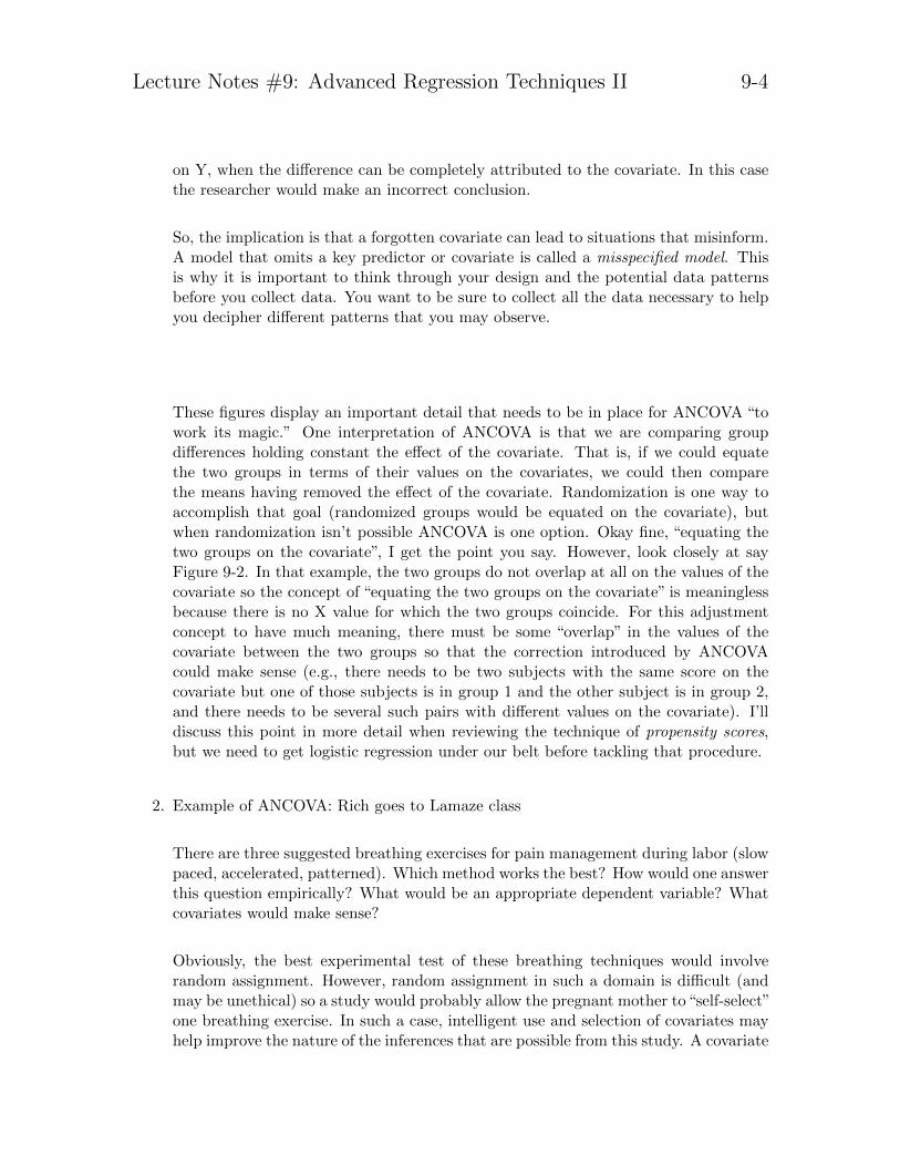
on Y, when the difference can be completely attributed to the covariate. In this casethe researcher would make an incorrect conclusion.

So, the implication is that a forgotten covariate can lead to situations that misinform.A model that omits a key predictor or covariate is called a misspecified model. Thisis why it is important to think through your design and the potential data patternsbefore you collect data. You want to be sure to collect all the data necessary to helpyou decipher different patterns that you may observe.

These figures display an important detail that needs to be in place for ANCOVA “towork its magic.” One interpretation of ANCOVA is that we are comparing groupdifferences holding constant the effect of the covariate. That is, if we could equatethe two groups in terms of their values on the covariates, we could then comparethe means having removed the effect of the covariate. Randomization is one way toaccomplish that goal (randomized groups would be equated on the covariate), butwhen randomization isn’t possible ANCOVA is one option. Okay fine, “equating thetwo groups on the covariate”, I get the point you say. However, look closely at sayFigure 9-2. In that example, the two groups do not overlap at all on the values of thecovariate so the concept of “equating the two groups on the covariate” is meaninglessbecause there is no X value for which the two groups coincide. For this adjustmentconcept to have much meaning, there must be some “overlap” in the values of thecovariate between the two groups so that the correction introduced by ANCOVAcould make sense (e.g., there needs to be two subjects with the same score on thecovariate but one of those subjects is in group 1 and the other subject is in group 2,and there needs to be several such pairs with different values on the covariate). I’lldiscuss this point in more detail when reviewing the technique of propensity scores,but we need to get logistic regression under our belt before tackling that procedure.

2. Example of ANCOVA: Rich goes to Lamaze class

There are three suggested breathing exercises for pain management during labor (slowpaced, accelerated, patterned). Which method works the best? How would one answerthis question empirically? What would be an appropriate dependent variable? Whatcovariates would make sense?

Obviously, the best experimental test of these breathing techniques would involverandom assignment. However, random assignment in such a domain is difficult (andmay be unethical) so a study would probably allow the pregnant mother to“self-select”one breathing exercise. In such a case, intelligent use and selection of covariates mayhelp improve the nature of the inferences that are possible from this study. A covariate


Figure 9-2: ANCOVA with two groups. The slopes are the same for the two groups but theintercepts differ. In this example, there is no difference between the two unadjusted groupmeans (as indicated by the horizontal line going through the two ovals). That is, bothgroups have the same unadjusted mean value on Y. However, performing an ANCOVAyields a group difference in adjusted means, as indicated by the difference in the interceptbetween the two lines. The reason is that both groups differ on the value of the covariate.


Figure 9-3: ANCOVA with two groups. The slopes and intercepts are the same for thetwo groups. In this example, the ANCOVA reveals no difference in adjusted group meansbecause the intercept is the same for each group. Thus, any initial difference on Y canbe explained by the covariate. Once the effect of the covariate is removed, then no groupdifference remains.


Figure 9-4: ANCOVA with two groups. The slopes are the same but the intercepts differ.In this example, the ANCOVA reveals a group difference in adjusted means even thoughthe mean value of the covariate is the same for each group.


is, in a sense, a way to control statistically for external variables rather than controlfor them experimentally as in a randomized block design. In some domains, statisticalcontrol is the only option one has.

3. Testing for Parallelism in ANCOVA

The assumptions for ANCOVA are the same as in the usual regression. There is oneparallelismassumption

additional assumption: the slope corresponding to the covariate is the same acrossall groups. Look at Eq 9-1–there is nothing there that allows each group to have adifferent slope for the covariate. Hence, the assumption that the slopes for each groupare equal.

The equality of slopes assumption is easy to test. Just run a second regression thatincludes the interaction between the covariate and the dummy code. For example, totest parallelism for a model having one covariate and two groups, one would run thefollowing regression

Y = β0 + β1C + β2X + β3CX (9-2)

where CX is simply the product of C and X. The only test you care about in Eq 9-2is whether or not β3 is statistically different from zero. The interaction slope β3 is theonly test that is interpreted in this regression because the covariate is probably corre-lated with the grouping variable. Recall that sometimes the presence of an interactionterm in the model makes the main effects uninterpretable due to multicolinearity. Cen-tering the predictor variables will help make the main effect interpretable. But keep inmind that the regression in Equation 9-2 is for testing the parallel slope assumption,so all we care about is the interaction. Hence, for this regression centering isn’t reallyneeded, but everything is fine if you center.

If the interaction in Equation 9-2 is not significant, then parallelism is okay; but if β3is statistically significant, then parallelism is violated because there is an interactionbetween the covariate and the grouping variable.2

Most of my lecture notes on ANCOVA make use of the REGRESSION command inSPSS. MANOVA and GLM are two other SPSS commands that also handle covari-ates. I noticed a strange difference between the MANOVA and GLM commands: theyeach handle covariates differently. The MANOVA command behaves nicely and au-tomatically centers all predictors (regardless of whether they are expressed as factorsthrough BY or expressed as covariates through WITH). The GLM command thoughdoesn’t center the covariates (those variables after the WITH), but does for factors

2Of course, issues of power come into play when testing the parallelism assumption—with enough subjectsyou will typically reject the assumption even if the magnitude of the parallelism violation is relatively small.


specified through the BY subcommand. So while GLM does automatically test theparallelism assumption by fitting interactions of covariate and predictor, it doesn’tcenter the variables so the analyses for the main effects are off. GLM does center thefactors in the usual factorial (those using the BY command)—basically everything af-ter BY is centered but everything after WITH is not3. Of course, only discrete factorsmake sense to include as part of the BY subcommand, not continuous predictors. Ihave had several cases in collaborative work where a couple of us rerun the analysesand we find differences in our results usually due to subtle differences like one of usused BY and the other WITH, or one of us used one command in SPSS/R and theother used another command in SPSS/R that should have yielded the same answerbut the commands differ in small ways such as how they handle order of entry in aregression, centering, etc.

The basic lesson here is if you want to test any interaction, and in the case of ANCOVAyou do want to test the parallelism assumption by testing the interaction term, thencenter or you could get incorrect results for the main effects just by some weird detailof the particular program you are using (such as MANOVA or GLM in SPSS but alsowith R commands) and subtle differences between whether you use the BY or theWITH command. Don’t trust the stat package to do the right thing. Get in the habitof centering all your variables whenever you include interaction terms of any kind.This way you can interpret the main effects even in the presence of a statisticallysignificant interaction.

If you do find a violation of the parallelism assumption, then alternative proceduressuch as the Johnson-Neyman technique can be used (see Rogosa, 1980, Psychologi-cal Bulletin, for an excellent discussion). Maxwell and Delaney also discuss this intheir ANCOVA chapters. Obviously, if the slopes differ, then it isn’t appropriate totalk about a single effect of the categorical variable because the effect depends on thelevel of the covariate. The more complicated techniques amount to finding tests ofsignificance for the categorical predictor conditional on particular values of the covari-ate. They are similar to what we saw in Lecture Notes #8 for testing interactions inregression.

To understand Equation 9-2 it is helpful to code the groups denoted by variable X aseither 0 or 1 (i.e., dummy codes) and write out the equation. Note that when X = 0Equation 9-2 reduces to a simple linear regression of the dependent variable on thecovariate with intercept β0 and slope β1C. However, when X = 1 Equation 9-2 is alsoa simple linear regression of the dependent variable on the covariate but the interceptis (β0 + β2) and the slope is (β1 + β3)C. Thus, β3 is a test of whether the slope is thesame in both groups and β2 is a test of whether the intercept is the same for bothgroups. For instance, if β3 = 0, then the slope in each group is the same but if β3 6= 0,

3The MIXED command in SPSS suffers from the same issue of how it handles BY and WITH, be carefulwith that command too.


then the slopes differ across the two groups.

More complicated ANCOVA designs can have more than one covariate and more thantwo groups. To get more than one covariate just include each covariate as a separatepredictor. To get more than two groups just do the usual dummy coding (or contrastcoding or effects coding). Here is an example with two covariates (C1 and C2) andfour groups (needing three dummy codes or contrast codes—X1, X2, and X3)

Y = β0 + β1C1 + β2C2 + β3X1 + β4X2 + β5X3 (9-3)

This model is testing whether there is a difference between the four groups once thevariability due to the two covariates has been removed. Thus, we would be interestedin comparing the full model (with all five predictors) to the reduced model (omittingthe three dummy codes). This “increment in R2” test corresponds to the researchquestion: do the grouping variables add a significant amount to the R2 over andabove what the covariates are already accounting for. If dummy codes are used, theincrement in R2 test described above tests the omnibus hypothesis correcting for thetwo covariates. It is also possible to replace the three dummy codes with a set ofthree orthogonal contrasts. The contrast codings would allow you to test the uniquecontribution of the contrasts while at the same time correcting for the variability of thecovariates, thus reducing the error term. The t-tests corresponding to the βs for eachcontrast correspond to the test of the contrast having accounted for the covariate (i.e.,reducing the error variance in the presence of the covariates). That is, the individualβ’s correspond the tests of significance for that particular contrast (having correctedfor the covariate). Again, the usual regression/ANOVA assumptions hold as wellas the equality of slopes assumption, which permits one to interpret the results ofANCOVA in terms of adjusted means. Further, there should be good overlap acrossboth the covariates for each group. If some covariates are completely nonoverlappingacross the groups, then there isn’t much meaning to “controlling” for the covariates,as we saw earlier in these lecture notes in the case of one covariate.

4. Two ANCOVA examples

Here I show the effects of a covariate reducing noise (MSE) as compared to an analysisof the group differences without the covariate (i.e., using, for example, the ONEWAYcommand). The first column is the grouping code, the second column is the covariate,and the third column is the dependent variable.

1 5 61 3 41 1 01 4 31 6 7


2 2 12 6 72 4 32 7 82 3 2

data list file=’data’ free/ grp covar dv.

plot format = regression/plot= dv with covar by grp.

regression variables = grp covar dv/statistics r anova coef ci/dependent dv/method=enter covar grp.

oneway dv by grp(1,2).

Multiple R .97188 Analysis of Variance

R Square .94456 DF Sum of Squares Mean Square

Adjusted R Square .92872 Regression 2 65.08000 32.54000

Standard Error .73872 Residual 7 3.82000 .54571

F = 59.62827 Signif F = .0000

Variable B SE B 95% Confdnce Intrvl B Beta T Sig T

COVAR 1.425000 .130589 1.116206 1.733794 .984698 10.912 .0000

GRP -.655000 .473735 -1.775203 .465203 -.124768 -1.383 .2093

(Constant) -.760000 .848730 -2.766923 1.246923 -.895 .4003

Variable DV

By Variable GRP

ANALYSIS OF VARIANCE

SUM OF MEAN F F

SOURCE D.F. SQUARES SQUARES RATIO PROB.

BETWEEN GROUPS 1 .1000 .1000 .0116 .9168

WITHIN GROUPS 8 68.8000 8.6000

TOTAL 9 68.9000

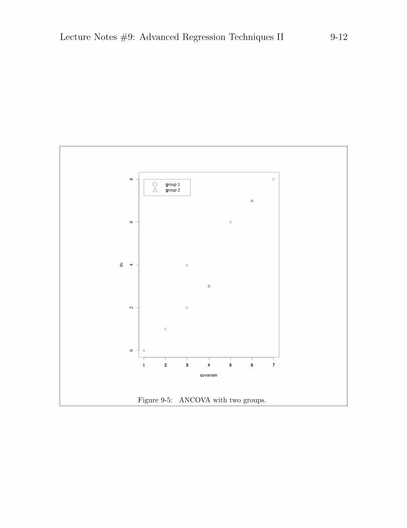
This version illustrates how a slight change in the arrangement of the plot changesthe ANCOVA result. It is very important to check the graph before performingthe ANCOVA so you know exactly what the covariate is doing. Note that in theseexamples parallelism holds. One should always check that parallelism holds (i.e., thereis no interaction between the grouping variable and the covariate) before proceedingwith the analysis of covariance.


covariate�

dv

1 2�

3�

4�

5�

6�

7�

02

46

8

group 1�

group 2�

Figure 9-5: ANCOVA with two groups.


DATA SET #2 (JUST CHANGED THE THIRD COLUMN FOR TREATMENT #1)1 5 111 3 91 1 51 4 81 6 122 2 12 6 72 4 32 7 82 3 2

data list file=’data2’ free/ grp covar dv.

plot format = regression/plot= dv with covar by grp.

regression variables = grp covar dv/statistics r anova coef ci/dependent dv/method=enter covar grp.

oneway dv by grp(1,2).

Multiple R .98477 Analysis of Variance

R Square .96978 DF Sum of Squares Mean Square

Adjusted R Square .96114 Regression 2 122.58000 61.29000

Standard Error .73872 Residual 7 3.82000 .54571

F = 112.31152 Signif F = .0000

Variable B SE B 95% Confdnce Intrvl B Beta T Sig T

COVAR 1.425000 .130589 1.116206 1.733794 .727008 10.912 .0000

GRP -5.655000 .473735 -6.775203 -4.534797 -.795297 -11.937 .0000

(Constant) 9.240000 .848730 7.233077 11.246923 10.887 .0000

ANALYSIS OF VARIANCE

SUM OF MEAN F F

SOURCE D.F. SQUARES SQUARES RATIO PROB.

BETWEEN GROUPS 1 57.6000 57.6000 6.6977 .0322

WITHIN GROUPS 8 68.8000 8.6000

TOTAL 9 126.4000

The identical analysis can be done within the MANOVA command. The covariateis added at the first line after the keyword “with”. The PMEANS subcommand ishelpful because it gives the adjusted means (i.e., what the ANCOVA predicts in theregression) when the value of the covariate is set equal to the mean of the covariate. Forexample, the mean of the covariate (collapsing over all groups) is 4.1. The predictedmean on the DV for group 1 using the regression estimates from the previous regression


covariate�

dv

1 2�

3�

4�

5�

6�

7�

24

68

1012

group 1�

group 2�

Figure 9-6: ANCOVA with two groups.


above is

Y = β0 + β1X + β2G (9-4)

= 9.24 + (1.425)(4.1) + (−5.665)(1) (9-5)

= 9.4275 (9-6)

For group 2, it’s the same equation except that G=2 rather than G=1 is entered intothe regression, so we have

Y = β0 + β1X + β2G (9-7)

= 9.24 + (1.425)(4.1) + (−5.665)(2) (9-8)

= 3.7725 (9-9)

In the following output, the F tests for the covariate and the grouping variable in thesource table are identical to the square of the t-tests given in the previous regressionrun (i.e., 10.9122 and -11.9372). The PMEANS subcommand produces the predictedmeans of 9.4 and 3.77 as I computed manually from the regression equation above.

manova dv by grp(1,2) with covar/pmeans tables(grp)/design grp.

Tests of Significance for DV using UNIQUE sums of squares

Source of Variation SS DF MS F Sig of F

WITHIN+RESIDUAL 3.82 7 .55

REGRESSION 64.98 1 64.98 119.07 .000

GRP 77.76 1 77.76 142.49 .000

(Model) 122.58 2 61.29 112.31 .000

(Total) 126.40 9 14.04

R-Squared = .970

Adjusted R-Squared = .961

Regression analysis for WITHIN+RESIDUAL error term

--- Individual Univariate .9500 confidence intervals

Dependent variable .. DV

COVARIATE B Beta Std. Err. t-Value Sig. of t Lower -95% CL- Upper

COVAR 1.4250000000 .7270081448 .13059 10.91207 .000 1.11621 1.73379

Adjusted and Estimated Means

Variable .. DV

Factor Code Obs. Mean Adj. Mean Est. Mean Raw Resid. Std. Resid.

GRP 1 9.00000 9.42750 9.00000 .00000 .00000

GRP 2 4.20000 3.77250 4.20000 .00000 .00000


Combined Adjusted Means for GRP

Variable .. DV

GRP

1 UNWGT. 9.42750

2 UNWGT. 3.77250

It is possible to test the equality of slope assumption in the MANOVA command bythis trick. The design line enters the two main effects and the interaction, and there isthis new subcommand ANALYSIS, which I don’t want to get into here because it ispretty esoteric. The test of the interaction term appears in the ANOVA source table.The only thing you care about in this output is the significance test for the interaction.Here is my preferred syntax for testing the interaction between the covariate and thegrouping variable in the MANOVA command:

manova dv by grp(1,2) with covar

/pmeans tables(grp)

/analysis dv

/design grp covar grp by covar.

If the equality of slope assumption is rejected, then you can fit an ANCOVA-like modelthat permits the two groups to have different slopes using the following syntax (thecovariate is “nested” within the grouping code). But my own preference is to stickwith the previous analysis that uses an interaction. The following approach, though,is more commonly accepted. The F test for the grouping variable is identical for bothapproaches and the MSE term is also identical (as are the “adjusted means,” which areidentical to the observed means). The two approaches differ in that the interactionapproach keeps the main effect for covariate and the interaction separate, whereas thefollowing approach lumps the sum of squares for interaction and covariate main effectinto a single omnibus test (and you know how I feel about omnibus tests). Here is themore common syntax, though not my favorite way of testing the interaction:

manova dv by grp(1,2) with covar

/pmeans tables(grp)

/analysis dv

/design covar within grp, grp.

5. A Standard ANCOVA Misunderstanding

In Lecture Notes 8 I reviewed the definitions of part and partial correlation. I alsoshowed how one could estimate part and partial correlations through regressions on


residuals. Recall that the key issue was that the other predictors are removed fromthe predictor of interest, and then the residuals of that predictor are correlated withthe dependent variable.

ANCOVA follows that same logic. The variance of the covariate is removed from thegrouping variable and the residuals from that regression are used as the predictor ofthe dependent variable. Thus, one can interpret the analysis as one of purging thelinear effect of the covariate from the predictor variable. Many users though havethe misconception that ANCOVA purges the covariate from the dependent variable.

Model notation should make all this clearer. ANCOVA compares the first model tothe second model (X is the covariate and G is the grouping variable):

Y = β0 + β1X + ε

Y = β0 + β1X + β2G+ ε

with the focus being on the t-test of β2, the slope of the grouping variable. This isidentical in spirit to first running a regression with G as the dependent variable andthe covariate X as the sole predictor, storing the residuals, and then correlating thoseresiduals with the dependent variable Y.

ANCOVA purges the covariate from the predictor not the dependent variable.

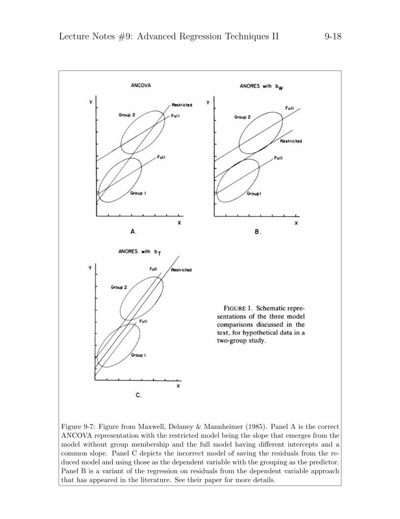
Maxwell et al (1985) have a nice paper explaining these misunderstandings, with someequations, a numerical example and a tutorial figure, which I reproduce in Figure 9-7.

The correct interpretation of ANCOVA follows directly from the development of thepart and partial correlations I introduced in Lecture Notes #8, where the inclusion ofadditional predictors modifies the other predictors already in the regression equationrather than modifying the dependent variable (which is the misunderstanding com-monly found in the literature). Basically, ANCOVA and blocking factors control forother predictors and do not “adjust” the dependent variable.

6. General observations about ANCOVA

ANCOVA is a way to remove the linear effect of a nuisance variable through a statis-tical model. These nuisance variables are not manipulated. This is probably the maindifference between how ANCOVA and randomized block designs are usually imple-mented. The former controls through statistical analysis. The latter design controlsfor blocking variables through experimental control, and that experimental controlwas used to reduce the error term. Most ANCOVA applications do not offer the


Figure 9-7: Figure from Maxwell, Delaney & Mannheimer (1985). Panel A is the correctANCOVA representation with the restricted model being the slope that emerges from themodel without group membership and the full model having different intercepts and acommon slope. Panel C depicts the incorrect model of saving the residuals from the re-duced model and using those as the dependent variable with the grouping as the predictor.Panel B is a variant of the regression on residuals from the dependent variable approachthat has appeared in the literature. See their paper for more details.


luxury of experimental manipulation and adjusting for nuisance through ANCOVA isabout the only way to deal with nuisance variables.

It is possible to mix ANCOVA with everything we discussed this term. For instance,it is possible to add a naturally occurring covariate to a randomized block design (oreven a latin square design). In the case of a randomized design with a covariate, thereare two nuisance, or blocking variables—one that is manipulated and one that isn’t.There could be random or nested effects; there could be repeated measures where thecovariate is also repeated. Anything we’ve done so far can be extended to includecovariates.

If a variable is relevant in your data but you ignore it as a covariate and just run aregular ANOVA or regression, you have what is called a misspecified model. A modelthat is misspecified could seem to be violating some assumptions.

For example, it is possible that what looks to you as a violation of the equality ofvariance assumption could really be due to a misspecified model. The presence of acovariate that isn’t included in the model could influence the cell variances and makeit appear that there are unequal variances.

Another example is that there could be heterogeneity in the treatment effect. Differentpeople respond differently to the treatment effect α so that the treatment isn’t aconstant within a group as assumed by ANOVA (recall that the treatment effect α fromLecture Notes #2 is constant for all subjects in the same condition). If you happento have measured the covariate that is related to this heterogeneity of treatmentresponse, then the inclusion of that covariate in the ANOVA/regression model wouldeliminate the source of unequal variances. Note that this is a completely differentway of addressing the equality of variance assumption than we saw last semester (notransformation, no Welch, no nonparametric tests; just include the right covariate inthe model).

The basic idea is that ANOVA assumes the treatment effect is a constant for everycase in a cell. However, ANCOVA allows the treatment effect to vary as a functionof the covariate; in other words, ANCOVA allows cases within the same treatmentgroup to have different effects and so is one way to model individual differences. Twoexcellent papers by Byrk and Raudenbush (1988, Psychological Bulletin, 104, 396-04)and Porter and Raudenbush (1987, Journal of Counseling Psychology, 34, 383-92) de-velop this point more generally. Extensions to random effects regression slopes (whereeach subject has his own slope and intercept) allows for a more complete descriptionof individual differences in regression. This is handled through multilevel models withmany applications including growth curve analysis as used in developmental psychol-ogy. We touched on multilevel models briefly last semester (e.g., nested effects) andwe will cover this in more detail later this semester.


7. The Big Picture: Why Do We Care About the General Linear Model?

We have now seen four advantages to performing hypothesis tests in terms of thegeneral linear model. The general linear modelbenefits of the

general linearmodel

(a) Connects regression and ANOVA, providing a deeper understanding of ANOVAdesigns

(b) Provides the ability to perform residual analysis (examine how the model isgoing wrong, gives hints about how to correct misspecified models and violationsof assumptions, allows one to examine the effects of outliers, allows one to seewhether additional variables will be useful to include in the model)

(c) Allows one to combine what has traditionally been in the domain of ANOVA(categorical predictor variables) with what has traditionally been in the domainof regression analysis (continuous predictor variables) to create new tests suchas ANCOVA

(d) Provides a foundation on which (almost) all advanced statistical techniques inpsychology are based (e.g., principal components, factor analysis, multivariateanalysis of variance, discriminant analysis, canonical correlation, time series anal-ysis, log-linear analysis, classical multidimensional scaling, structural equationmodeling, multilevel modeling)

The first three points will have tremendous impact on the quality of your data analysis(deeper understanding of ANOVA, ability to talk intelligently about your model andits shortcomings, and, whenever possible, include covariates to reduce the randomerror).

Yes, it is more work in SPSS to get the dummy codes (or effect codes or contrast codes)into a regression analysis compared to the relatively simple ONEWAY, ANOVA, andMANOVA commands, but the benefits are worth it. It won’t be long before SPSSprovides easy routines for creating dummy, effects, and contrast codes (competitorssuch as R and SAS already have built-in functions that automatically create the propercodes in a regression), but I have been waiting for several years.

8. Binary data

The general linear model can be extended to distributions that are nonnormal. A com-monly occurring nonnormal distribution is the binomial. There are situations when


the dependent variable consists of 0’s and 1’s and one is interested in the number of1s per group (or equivalently, the proportion). Note that this differs from dummycodes that are predictors—we are now talking about the dependent variable being0 or 1. This means that the dependent variable is nonnormal. The dummy codeswe encountered when connecting ANOVA and regression were predictors not depen-dent variables and no distributional assumptions were made about those predictors.Computer programs exist that permit one to use the same command as you wouldfor regression but change the distribution of the dependent variable (e.g., normal,binomial, Poisson). SPSS though uses a different command, the GENLIN command.

Here I’ll cover some basics about data that follow a binomial distribution. I’ll denotethe sample proportion as p and the population proportion that p estimates as ρ (Greekletter rho). The variance of the sampling distribution of p isvariance of a

proportion

p (1-p)

N(9-10)

where N is the sample size that went into the computation of that sample estimatep. The square root of this variance is the standard error of p. Note something veryimportant about the standard error of p: it is related to the value of p. Thus, iftwo groups have different proportions, then it is possible for the two groups to havedifferent variances. I say possible because the standard error is symmetric aroundthe proportion .5. So, the proportions .2 and .8 have the same variance, but theproportions .1 and .7 (which also have a difference of .6) each have different variances.This creates a major problem for our standard approach because if the standarderror depends on p we cannot make the equality of variance assumption. If groupshave different proportions, then they likely have different variances and the equalityof variance assumption is violated before we do anything. So other procedures areneeded and we turn to a few of them.can’t make the

equal varianceassumptionwithproportions Another complication when dealing with proportions is that the regression model

needs to be constrained to not produce out of bounds values. That is, it wouldn’tmake much sense to have Y from the structural model be -23 or 1.3 because proportionsmust be between 0 and 1, inclusive. Also, observed proportions at the boundaries 0or 1 can wreak havoc if one blindly applies Equation 9-10 because the standard errorof those proportions is 0. The problem of “division by zero” occurs when you dividean estimate by it’s standard errors of zero.

(a) Comparing two binomial proportions—Chi-square test

You’ve probably heard about the χ2 contingency table test. It appears in almostevery introductory statistics textbook. It can be used to test two proportions.The test can be used, for instance, to test whether the proportion in group Adiffers from the proportion in group B.


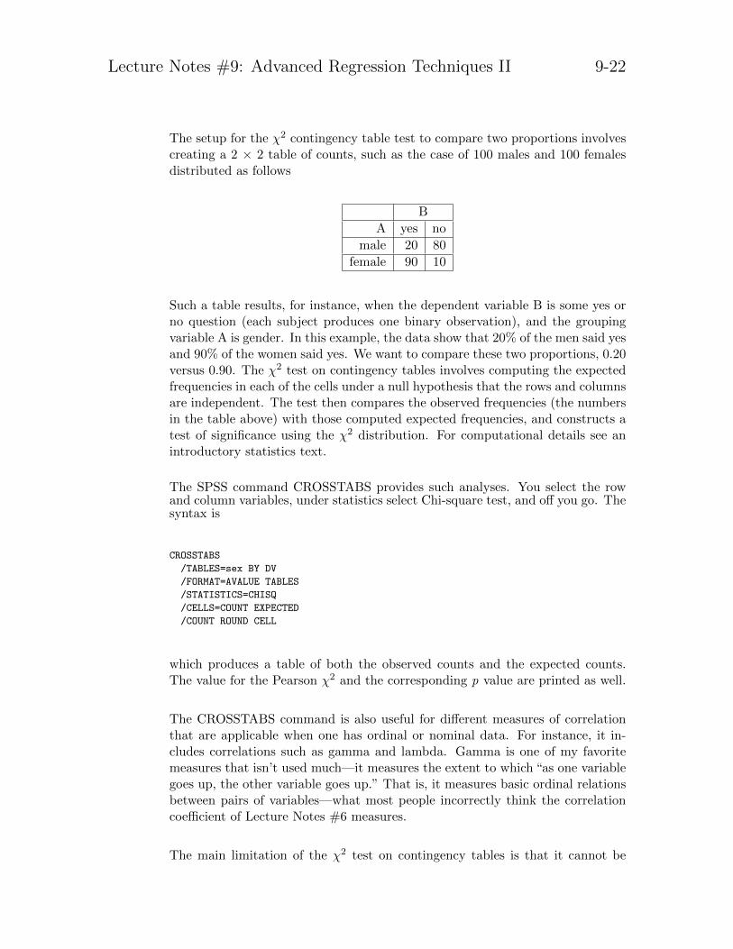
The setup for the χ2 contingency table test to compare two proportions involvescreating a 2 × 2 table of counts, such as the case of 100 males and 100 femalesdistributed as follows

B

A yes no

male 20 80

female 90 10

Such a table results, for instance, when the dependent variable B is some yes orno question (each subject produces one binary observation), and the groupingvariable A is gender. In this example, the data show that 20% of the men said yesand 90% of the women said yes. We want to compare these two proportions, 0.20versus 0.90. The χ2 test on contingency tables involves computing the expectedfrequencies in each of the cells under a null hypothesis that the rows and columnsare independent. The test then compares the observed frequencies (the numbersin the table above) with those computed expected frequencies, and constructs atest of significance using the χ2 distribution. For computational details see anintroductory statistics text.

The SPSS command CROSSTABS provides such analyses. You select the rowand column variables, under statistics select Chi-square test, and off you go. Thesyntax is

CROSSTABS

/TABLES=sex BY DV

/FORMAT=AVALUE TABLES

/STATISTICS=CHISQ

/CELLS=COUNT EXPECTED

/COUNT ROUND CELL

which produces a table of both the observed counts and the expected counts.The value for the Pearson χ2 and the corresponding p value are printed as well.

The CROSSTABS command is also useful for different measures of correlationthat are applicable when one has ordinal or nominal data. For instance, it in-cludes correlations such as gamma and lambda. Gamma is one of my favoritemeasures that isn’t used much—it measures the extent to which “as one variablegoes up, the other variable goes up.” That is, it measures basic ordinal relationsbetween pairs of variables—what most people incorrectly think the correlationcoefficient of Lecture Notes #6 measures.

The main limitation of the χ2 test on contingency tables is that it cannot be


generalized to perform tests on several proportions. For example, if you havea factorial design, with a proportion as the cell mean and you want to test formain effects, interactions and contrasts, the standard χ2 test on contingencytables won’t help you. At best, the χ2 contingency table test gives you anomnibus test saying that at least one of the observed proportions is differentfrom the others, much like the omnibus F in a oneway ANOVA. (You have todo some tricks, which aren’t implemented in most computer programs, to getanything useful out of the χ2 contingency table test). Also, χ2 contingency tableanalysis doesn’t generalize readily to include things like covariates. So, insteadI’ll present a different approach—logistic regression—that pretty much allowsyou accomplish all the machinery of regression that we have covered so far butusing binary data (i.e., assuming binary data rather than normally distributeddata).

(b) Comparing two binomial proportions—logistic regression

There are several alternative formulations. Here I will present one, logistic re-gression, because it is the most popular. It is not necessarily the best test but Ipresent it because it is the most common. If you are interested in learning moreabout alternative formulations, I can make a manuscript available that goes intomore detail including some Bayesian arguments.

I’ll first present logistic regression for the simple problem of comparing two pro-portions. First, I need to review some of the building blocks. Logistic regressionoperates on the “logit” (aka log odds) rather than the actual proportion. A logitis defined as follows:logit

logit = logp

1− p(9-11)

In other words, divide p by (1-p), this ratio is known as “odds”, and take thenatural log (ln button on a calculator).

The asymptotic variance of a logit isvariance of thelogit

variance(logit) =1

Np(1− p)(9-12)

where N is the sample size and p is the proportion. The square root of thisvariance is the standard error of the logit. Note that the standard error of thelogit suffers the same problem as the standard error of the proportion because itis related to the value of the proportion and consequently we cannot make theequal variance assumption.

Throughout these lecture notes, I mean “natural log” when I say “logs”. On mostcalculators this is the “ln” button. Being consistent with the base is important


because the formula for the variance above (Equation 9-12) depends on the base.If log base 10 is used instead of the natural log, then the variance of the “logit” is

1ln(10)2Np(1−p) where ln is the natural log. Of course, the value of the logit itself

also depends on the base of the log and luckily the value of the logit and thestandard error of the logit are each influenced by the base in the same way sowhen one divides the two to form a Z test, the effect of the base cancels givingthe identical test result. To keep things simple, just stick with the natural log,the “ln” key on your calculator, and all the formulas presented in these lecturenotes will work.

What do we do when we can’t make the equal variance assumption? We canuse a basic result from Wald that approximates a normal distribution. In words,here is a sketch of the result: a test on a contrast can be approximated bydividing the contrast I with the square root of the standard error of the contrast.The difference here from what we did in Lecture Notes #1 is that we won’tmake the assumption of equal variances and we won’t correct using a Welch-likeprocedure. We rely on Wald’s proof that as sample size gets large, things behaveokay and the estimate divided by the standard error of the estimate follows anormal distribution4.

Let’s look at Wald’s test for the special case of comparing two logits. This testturns out to be asymptotically equivalent to the familiar χ2 test on contingencytables applied to testing two proportions. The null hypothesis is

population one logit - population two logit = 0 (9-13)

which is the same as the (1 -1) contrast on the logits. The I is

(1) logp1

1− p1+ (−1) log

p21− p2

(9-14)

where the subscripts on the proportion refer to group number. Under the assump-tion of independence (justified here because I have a between-subjects design andthe two proportions are independent), the standard error of this contrast is givenby

se(contrast) =

√1

N1p1(1− p1)+

1

N2p2(1− p2)(9-15)

that is, the square root of the sum of the two logit variances.

4I once checked this for Type I error rates with simulations and “sample size gets large” means thingsstart to work okay when sample sizes are about 25 or 30 for proportions between .1 and .9. For proportionscloser to 0 or 1, then the sample size needs to be more like 100. I only checked Type I error rates and notpower. It may be possible that to achieve adequate power, sample sizes need to be even greater. A questionto be answered another day. . . , but tractable. This could be good project for someone with a good calculusand linear algebra background interested in learning more about mathematical statistics and simulations.Takers?


Finally, the test of this contrast is given by

Z =I

se(contrast)(9-16)

where Z follows the standard, normal distribution. If Z is greater than 1.96 thenyou reject the null hypothesis using α = .05 (two-tailed).

(c) Testing contrasts with more than two proportions

This Wald test can be generalized to more than two proportions. Take any num-ber of sample proportions p1, . . . , pT and a contrast λ over those T proportions.Here are the ingredients needed for the Wald Z test. The value of I is (contrastweights applied to each logit, then sum the products)

I =T∑i=1

λi logpi

1− pi(9-17)

The standard error of the contrast is

se(contrast) =

√√√√ T∑i=1

λ2i1

Nipi(1− pi)(9-18)

Finally, the Wald Z test for the null hypothesis that population I = 0 is simply

I

se(contrast)(9-19)

Again, the critical value for this Z is 1.96. If the observed Z exceeds 1.96, thenthe null hypothesis that the population I is 0 can be rejected using α = .05(two-tailed).

This test is the proportion version of the test I presented in Lecture Notes #6 fortesting contrasts on correlations. Note the analogous structure. Instead of theFisher’s r-to-Z we take log odds. The standard errors are different, but everythingelse is pretty much the same.

(d) Example

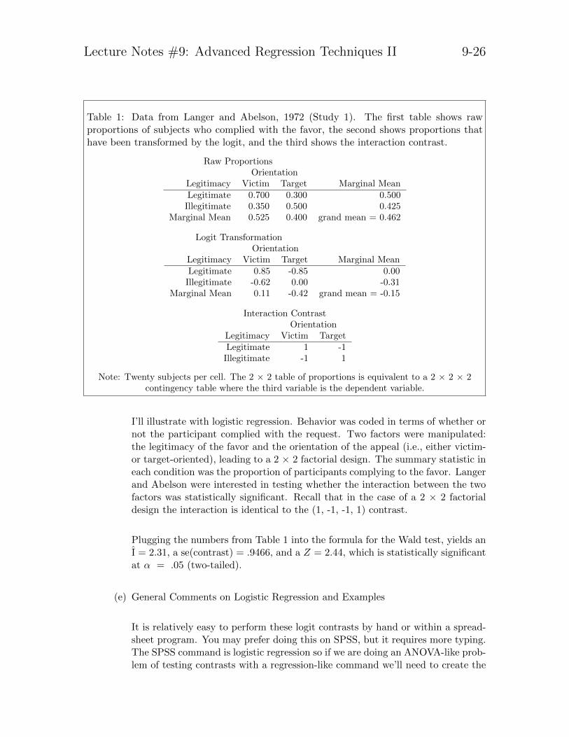
Table 1 shows an example taken from Langer and Abelson (1972), who studiedcompliance to a favor. They used a different analysis than logistic regression but


Table 1: Data from Langer and Abelson, 1972 (Study 1). The first table shows rawproportions of subjects who complied with the favor, the second shows proportions thathave been transformed by the logit, and the third shows the interaction contrast.

Raw ProportionsOrientation

Legitimacy Victim Target Marginal MeanLegitimate 0.700 0.300 0.500

Illegitimate 0.350 0.500 0.425Marginal Mean 0.525 0.400 grand mean = 0.462

Logit TransformationOrientation

Legitimacy Victim Target Marginal MeanLegitimate 0.85 -0.85 0.00

Illegitimate -0.62 0.00 -0.31Marginal Mean 0.11 -0.42 grand mean = -0.15

Interaction ContrastOrientation

Legitimacy Victim TargetLegitimate 1 -1

Illegitimate -1 1

Note: Twenty subjects per cell. The 2 × 2 table of proportions is equivalent to a 2 × 2 × 2contingency table where the third variable is the dependent variable.

I’ll illustrate with logistic regression. Behavior was coded in terms of whether ornot the participant complied with the request. Two factors were manipulated:the legitimacy of the favor and the orientation of the appeal (i.e., either victim-or target-oriented), leading to a 2 × 2 factorial design. The summary statistic ineach condition was the proportion of participants complying to the favor. Langerand Abelson were interested in testing whether the interaction between the twofactors was statistically significant. Recall that in the case of a 2 × 2 factorialdesign the interaction is identical to the (1, -1, -1, 1) contrast.

Plugging the numbers from Table 1 into the formula for the Wald test, yields anI = 2.31, a se(contrast) = .9466, and a Z = 2.44, which is statistically significantat α = .05 (two-tailed).

(e) General Comments on Logistic Regression and Examples

It is relatively easy to perform these logit contrasts by hand or within a spread-sheet program. You may prefer doing this on SPSS, but it requires more typing.The SPSS command is logistic regression so if we are doing an ANOVA-like prob-lem of testing contrasts with a regression-like command we’ll need to create the


dummy codes (or effects codes or contrasts codes) like I showed you before. Thismeans that to test contrasts using the logistic regression command in SPSS youneed to enter in lots and lots of extra codes, or use if-then statements in a cleverway5.

Here are the Langer & Abelson data coded for the SPSS logistic regression. Dataneed to be entered subject by subject. The first column is the grouping code (1-4), one main effect contrast for victim/target, the second main effect contrast forthe legitimacy manipulation, the interaction contrast and the dependent variable(1=compliance, 0=no compliance).

The syntax of the LOGISTIC command is similar to that of the REGRES-SION command. The dependent variable is specified in the first line, then the/method=enter lists all the predictor variables. The structural model beingtested by this syntax is

logit(p) = β0 + β1me.vt + β2me.legit + β3interact (9-20)

Note that the structural model is modelling the logit rather than the raw pro-portion, so its structural model is additive in the log odds scale.

I illustrate by presenting the entire dataset with codes entered directly into thefile. The first column is the group code (useful for a later demonstration);columns 2, 3 and 4 are main effects and interaction contrast codes; column 5lists the dependent variable.

data list free/ group me.vt me.legit interact dv.

begin data

1 1 1 1 1

1 1 1 1 1

1 1 1 1 1

1 1 1 1 1

1 1 1 1 1

1 1 1 1 1

1 1 1 1 1

1 1 1 1 1

1 1 1 1 1

1 1 1 1 1

1 1 1 1 1

1 1 1 1 1

1 1 1 1 1

5The SPSS logistic regression command is actually quite general. The command will accept predictorsthat are “continuous”, unlike the simple method I present here that only tests contrasts so in regressionparlance uses categorical predictors rather than continuous predictors. This feature could be useful in someapplications, e.g., regressing teenage pregnancy (coded as “yes” or “no”) on GPA, parent’s salary, and theinteraction between GPA and parent’s salary. If you are interested more in how to perform regression-likeanalyses on binary data, I suggest that you take a more detailed course on categorical data analysis.


1 1 1 1 1

1 1 1 1 0

1 1 1 1 0

1 1 1 1 0

1 1 1 1 0

1 1 1 1 0

1 1 1 1 0

2 1 -1 -1 1

2 1 -1 -1 1

2 1 -1 -1 1

2 1 -1 -1 1

2 1 -1 -1 1

2 1 -1 -1 1

2 1 -1 -1 0

2 1 -1 -1 0

2 1 -1 -1 0

2 1 -1 -1 0

2 1 -1 -1 0

2 1 -1 -1 0

2 1 -1 -1 0

2 1 -1 -1 0

2 1 -1 -1 0

2 1 -1 -1 0

2 1 -1 -1 0

2 1 -1 -1 0

2 1 -1 -1 0

2 1 -1 -1 0

3 -1 1 -1 1

3 -1 1 -1 1

3 -1 1 -1 1

3 -1 1 -1 1

3 -1 1 -1 1

3 -1 1 -1 1

3 -1 1 -1 1

3 -1 1 -1 0

3 -1 1 -1 0

3 -1 1 -1 0

3 -1 1 -1 0

3 -1 1 -1 0

3 -1 1 -1 0

3 -1 1 -1 0

3 -1 1 -1 0

3 -1 1 -1 0

3 -1 1 -1 0

3 -1 1 -1 0

3 -1 1 -1 0

3 -1 1 -1 0

4 -1 -1 1 1

4 -1 -1 1 1

4 -1 -1 1 1

4 -1 -1 1 1

4 -1 -1 1 1

4 -1 -1 1 1

4 -1 -1 1 1

4 -1 -1 1 1

4 -1 -1 1 1

4 -1 -1 1 1

4 -1 -1 1 0

4 -1 -1 1 0

4 -1 -1 1 0

4 -1 -1 1 0

4 -1 -1 1 0

4 -1 -1 1 0

4 -1 -1 1 0


4 -1 -1 1 0

4 -1 -1 1 0

4 -1 -1 1 0

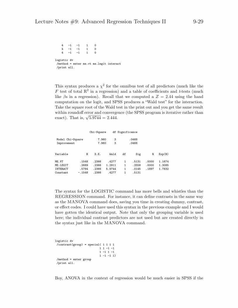
logistic dv

/method = enter me.vt me.legit interact

/print all.

This syntax produces a χ2 for the omnibus test of all predictors (much like theF test of total R2 in a regression) and a table of coefficients and t-tests (muchlike βs in a regression). Recall that we computed a Z = 2.44 using the handcomputation on the logit, and SPSS produces a “Wald test” for the interaction.Take the square root of the Wald test in the print out and you get the same resultwithin roundoff error and convergence (the SPSS program is iterative rather thanexact). That is,

√5.9744 = 2.444.

Chi-Square df Significance

Model Chi-Square 7.960 3 .0468

Improvement 7.960 3 .0468

Variable B S.E. Wald df Sig R Exp(B)

ME.VT .1548 .2366 .4277 1 .5131 .0000 1.1674

ME.LEGIT .2689 .2366 1.2911 1 .2558 .0000 1.3085

INTERACT .5784 .2366 5.9744 1 .0145 .1897 1.7832

Constant -.1548 .2366 .4277 1 .5131

The syntax for the LOGISTIC command has more bells and whistles than theREGRESSION command. For instance, it can define contrasts in the same wayas the MANOVA command does, saving you time in creating dummy, contrast,or effect codes. I could have used this syntax in the previous example and I wouldhave gotten the identical output. Note that only the grouping variable is usedhere; the individual contrast predictors are not used but are created directly inthe syntax just like in the MANOVA command.

logistic dv

/contrast(group) = special( 1 1 1 1

1 1 -1 -1

1 -1 1 -1

1 -1 -1 1)

/method = enter group

/print all.

Boy, ANOVA in the context of regression would be much easier in SPSS if the


REGRESSION command also had this feature of being able to define contrastson predictor variables!

It it a good idea to use the contrast=special command on ALL categorical vari-ables (even ones with only two levels). This tells the logistic command to treatthe variable correctly and helps guard against forgetting to treat categoricalvariables as categorical. Recall that when discussing anova in the context of re-gression (lecture notes 8), I brought up the issue that there should be as manypredictors for each variable as there are levels of that variable minus one.

The logistic command allows one to call a variable categorical, which further helpsclarify communication with the program. Below I’ve added the categorical sub-command. The output will be identical as above. The categorical subcommandis useful when you have lots of variables and you need to keep track of what is cat-egorical and what isn’t (you can write /categorical = LIST_OF_VARIABLES ).

logistic dv

/categorical group

/contrast(group) = special( 1 1 1 1

1 1 -1 -1

1 -1 1 -1

1 -1 -1 1)

/method = enter group

/print all.

On some versions of SPSS you may get a warning message saying that the firstrow in contrast=special was ignored (i.e., SPSS is ignoring the unit vector–nobig deal).

You can also use this simple syntax to specify ANOVAs as well (be sure to specifyall the main effects and interactions). Here is the syntax for a three way ANOVAwith factors A (four levels), B (two levels), and C (three levels):

logistic dv

/categorical A B C

/contrast(A) = special( 1 1 1 1

1 1 -1 -1

1 -1 1 -1

1 -1 -1 1)

/contrast(B) = special(1 1

1 -1)

/contrast(C) = special(1 1 1

0 1 -1

-2 1 1)

/method = enter A, B, C, A by B, A by C, B by C, A by B by C

/print all.


(f) Caveat: important issue of error variance.

One needs to be careful when comparing coefficients across logistic regressionmodels, or even coefficients across groups. The reason is that the error variancein logistic regression is a constant. Every logistic regression has the same errorvariance equal to π2

3 = 3.29. This means that as one adds more variablesto a logistic regression, the scale changes and a β in one regression is on adifferent scale than one in a different regression. This could make it look like aslope changed, or that slopes across groups differ, when in reality the differencemay be due to scale. This is not at all intuitive or obvious, and it has createdheadaches across many literatures where papers, for example, claim differencesbetween groups when it could just be an issue of different scales (an oranges andapples comparison). Traditional normally distributed regression does not havethis problem because the error sum of squares and the explained sum of squaresare both estimated from the data and must sum to the same amount—the sumof squares of the dependent variable.

9. Propensity scores

The concept of propensity scores is both new and powerful. It works well when thereare many covariates, it isn’t as restrictive as ANCOVA, it makes clear when there isor isn’t overlap in the covariate across the groups, and makes a very interesting useof logistic regression as a first step to remove the effect of covariate(s).

Let’s assume we have two groups and two covariates for this simple example. One runstwo regressions in propensity score analysis. The first regression is a logistic regressionwhere the binary code for group membership (0 and 1) representing the two groupsis the dependent variable and all covariates are the predictors. The purpose of thisregression is to get predicted values (the Ys) of group membership. That is, usethe covariates to predict actual group membership. Two subjects with the same orsimilar Y have the same “propensity” of being assigned to a particular group. Thesame propensity can occur with multiple combinations of covariates. More deeply, iftwo people have the same propensity score, they have the same “probability” of beingassigned by the covariates to the group. If one of those individuals is actually in onegroup and the other is in the second group, it is as though two individuals “matched”on the covariates by virtue of having the same propensity score were assigned todifferent groups. Not quite random assignment but an interesting way to conceptualizematching.

Second, you conduct a different regression that controls for the covariates. There areseveral ways one can do this. For building intuition I’ll first mention one method.Conduct a regular ANCOVA with the dependent variable of interest and the groupingvariable as the predictor, but don’t use the actual covariate(s) in this regression,


instead use the propensity score (the Ys) from the first regression as the sole covariate.This allows one “to equate” nonexperimental groups in a way that resembles randomassignment. But I mentioned that method just for intuition as it isn’t optimal; thisparticular version is not in favor and propensity score proponents would argue that itmisses the point of using propensity scores.

Instead, there are more complicated procedures for the second regression where thepropensity scores are used to create blocks (or strata), and then a randomized blockdesign is used rather than an ANCOVA with the grouped propensity scores playing therole of the blocking factor. There are many, many more sophisticated ways in whichone can match on propensity scores and this is currently a major topic of research.

There is a nice paper by D. Rubin on propensity scores in 1997, Annals of InternalMedicine, 127, 757-63, and now a complete book on the topic, Guo & Fraser (2010),Propensity Score Analysis. A paper by Shadish et al (2008, JASA) conducts anexperiment where subjects are either assigned into an experiment (randomly assignedto one of two treatments) or a nonrandomized experiment (they choose one of twotreatments). Overall results suggest that propensity score methods do not work aswell as one would have hoped in correcting for bias in the nonexperimental portionof the study (i.e., the self-selection bias that was studied in this paper); there are toomany ways to compute, calibrate, etc., propensity scores with little consensus on theoptimal approach. Propensity score approaches, do have a role at the study designstage if one wants to match subjects. If you can’t randomly assign in your researchdomain keep an eye out for new developments in the propensity score literature asthis is one of the more promising ideas in a long time, though as Shadish et al pointout it just isn’t there yet.

10. Time series

If time permits. . . . Okay, not funny if you are a time series aficionado.

We have already covered a major type of time series analyses when we did repeatedmeasures ANOVA in LN #6 and a little when I showed how to do a paired t test inthe context of regression (LN #8). There is much more to time series; I’ll cover somein class and will return later in the semester. The basic ideas:

(a) Smoothing

Sometimes data analysts like to smooth a time series to make it easier to un-derstand and find underlying patterns. There are many ways of smoothing timeseries data. Figure 10a shows some blood pressure data. The raw data (points)look jagged and don’t have much of a visible pattern, but a smoothed version


6080

100

120

140

160

Day

Blo

od P

ress

ure/

Hea

rt R

ate

86

142

62

F S S M TW T F S S M TW T F S S M TW T F S S M TW T F S S M TW T F S S M TW T F S S M TW T F S S M TW T F S S M TW T F S S M TW T F S S M T

Figure 9-8: Smoothing time series data. Blood pressure and heart rate of one subject.Horizontal lines are the means; curves are smoothed prediction models.

suggests a systematic, underlying pattern. Smoothed data can make it easier tosee patterns, but can also hide noisy data. I like to plot both data and modelfits.

(b) Correlated error

A key issue with time series is that the residuals are correlated. For example, anerror at time 1 could be related to the error at time 2, etc. There are several waysof dealing with correlated error, or the violation of the independence assumption.We saw a few of them when doing repeated measures. At one extreme we justignore the violation and pretend the data are independent. This amounts toa covariance matrix over time where all the off diagonals (covariance of time iwith time j) are zero. At the other extreme we allow all covariance terms tobe different and estimate them as parameters. This is what we did in repeatedmeasures under the “multivariate” form, also known as unstructured. This is


the method I advocated in the repeated measures section of the course becauseit bypasses pooling error terms so no need to make sphericity or compoundsymmetry assumptions. By focusing on contrasts in that setting we createdspecial error terms for each contrast and we didn’t have to make assumptionsabout the structure of the error covariance matrix.

Somewhere between those two extremes are several other options. In repeatedmeasures ANOVA we covered one, where we assumed compound symmetry, butthere are others. For example, one can assume a structure where adjacent timesare correlated but all other correlations are zero. There are many, many differenterror structures that one can assume and/or test in a data set; you can look atthe SPSS syntax help file for MANOVA or GLM for different assumptions onecan make on the correlated error term. The standard approach is to test theseapproaches against each other, settling on one approach that balances the fit ofthe data with the increase in extra parameters that need to be estimated. Thereis much work that can be done in this area and opportunity for developing newanalytic approaches.

(c) Dealing with correlated error

One approach to dealing with correlated error is to transform the problem toreduce the issue of a correlated error. The Kutner et al book goes into this detail.Essentially one takes a difference score of the Y variable, a difference score ofthe X variable (i.e., both are lag 1) and uses those “transformed” variables inthe regression instead of the raw variables. The difference score of lag 1 refersto using the score minus its previous time’s value (such as Y2 - Y1 where thesubscript denotes time). There are also variants of this approach where insteadof taking differences, one takes a weighted differences as in Y ′ = Yi+1 − ρYi. Adifference is still taken but the earlier time is weighted by ρ. If ρ = 1, then thisis the same as a lagged difference score6.

Another approach is to model the correlations directly. This can be done inseveral ways such as using random effects multilevel models, by using a general-ized least squares approach, by moving to different estimation procedures suchas GEE, or using some classic approaches involving variance components (gen-eralizations of the ANOVA concepts). Lots of options here. I’d say consensus isbuilding up in using multilevel models (aka random effect models like we saw inANOVA), which can be estimated with either traditional methods like we haveseen in this class or Bayesian approaches, and perhaps the GEE technique comingin second in some literatures like in public health.

6The idea of taking such lagged differences can begin to approximate derivatives. The difference of twolagged differences approximates a second derivative, etc. Such tools can come in handy when modelingnonlinear time series and can provide new insight into the interpretation of the parameters.


(d) Indices of correlated error

As we saw in the repeated measures world with the ε measure, there are variousapproaches to estimating the interdependence over time. The Durbin-Watson ap-proach is relatively common in time series. The D-W measure is the ratio of sum

of squared residual differences over the sum of squared residuals (

∑n

t=2(εt−εt−1)2∑ε2

).

Kutner et al provide a table on which to compare statistical significance of theD-W measure, which is based on the sample size and the number of predictorsin the regression equation. The D-W measure can then be used to make adjust-ments to the data to deal with the correlated temporal structure in an analogousway that a Welch or Greenhouse-Geiser makes adjustments. I don’t find thisapproach useful because correlated error comes with the territory of time series.It isn’t a problem with the data but a feature. I feel better modeling it directlyand trying to understand it.

(e) General frameworks

A general framework for working with time series data is called the ARIMAapproach. This allows correlated errors, lagged predictors, the ability to model“shocks”, and a whole host of other processes. There are entire textbooks andcourses just on ARIMA models, so this topic is way beyond the scope of thiscourse.

As I said earlier, a complete treatment of time series requires at least a semester course.I suggest taking such a course if you think you’ll need to do time series analyses inyour research. A key issue is how many time points you typically encounter. If youanalyze 3-8 time points per subject, then probably repeated-measures style procedures,including modern multilevel modeling approaches that we’ll cover later in the term,will suit you well. If you collect 100s or 1000s of data points per subject as onedoes in EEG, fMRI or with sensor data (fitbits, heart rate sensors, etc), then a moresophisticated time series course would be relevant for you.

In addition to statistical ways of analyzing time series data, there are also varioustechniques that are commonly used in engineering and in physics such as signal pro-cessing procedures like filtering, decompositions, convolutions, and other approachesthat have also been useful in social science data.

11. Even more general models

Over the last decade there has been a proliferation of models more general than thegeneral linear model. I list two here:


(a) Generalized Linear Model: allows distributions other than the normal; the userspecifies the underlying distribution (e.g., normal, binomial, Poisson, beta, etc.);the logic is the same as multiple regression but without the constraint that thedata be normal; the user needs to know, however, the distribution of the data; bygeneralizing the normal-normal plot to work with any theoretical distribution,the user can get a good handle on what the underlying error distribution is forthe data under study. For more detail see McCullough & Nelder, GeneralizedLinear Models.

Logistic regression is one example of a generalized linear model as is the usualregression with a normally distributed error term, but there are many moredistributions that fall under this family of techniques.

SPSS now implements the generalized linear model in GENLIM. R has the gen-eralized linear model in the glm() command.

There is even a more general model that allows random effects in the contextof the generalized linear model, sometimes called the generalized linear mixedmodel (GLMM). This allows you to do everything you already know how to dowith regression, extend it to nonnormal distributions like proportions and countdata, and also deal with random effects. An example where random effects isuseful is when you want each subject to have their own slope and intercept, asin latent growth models. The generality of the GLMM is that you can do thisfor any type of distribution in the family. This isn’t implemented in SPSS yet,though it is implemented in SAS, R, Stata, and a few other specialized programs.The R packages nlme and lme4 both handled GLMM models; there are also somespecialty packages in R that offer variations on the GLMM framework.

Finally, a different type of generalization is to let the program search for differenttypes of subjects, cluster subjects and then analyze the data based on thoseempirically derived clusters. This is useful, for instance, if you think there aredifferent classes, or clusters, of subjects such that within a cluster the slopesand intercept are the same but across clusters they differ. But you don’t knowthe clusters in advance. This technique, known as a mixture model, can helpyou find those clusters. This type of analysis is commonly used in marketingresearch to find empirically-defined market segments (groups of people who sharecommon slopes and intercept). It is also used in developmental psychology tocluster different growth curves, or trajectories (i.e., kids with similar growthpatterns). Once a cluster is in hand, then the cluster can be studied to see ifthere are variables that identify cluster membership. This technique can alsoinclude random effects so that not all members of the same cluster have theidentical slopes and intercepts. We’ll first need to cover clustering (LN #10),and then if there is time we can return to this technique at the end of the term.


The computational aspects of this type of technique are complex and requirespecialized algorithms that are very different from those based on the centrallimit theorem that we have used in this class. Plus we need to learn how towork with algorithms that offer numerical approximations (LN#10 and LN#11)before delving too deeply into mixture models.

(b) Generalized Additive Model: these are my favorite “regression-like” models be-cause they make so few assumptions. They are fairly new and statistical testsfor these procedures have not been completely worked out yet. An excellent ref-erence is Hastie & Tibshirani, Generalized Additive Models (GAM). Even thoughthey are new it turns out that there are several special cases of this more generalapproach that have been around for decades. This GAM framework providesa scientific justification for various techniques that have been lingering aroundwithout much theoretical meat.

These models are “nonparametric” in the sense that they try to find an optimalscaling for each variable in the equation for an additive equation (under a vari-ety of error models). Thus, one is scaling psychological constructs and runningregression simultaneously, so doing scaling, prediction, estimation and testing allin one framework. We won’t cover generalized additive models in this course. Wewill cover a cousin of this technique, monotonic regression, when we take up thetopic of multidimensional scaling in lecture notes #10. R has the function gam()and a growing list of packages that can fit algorithms in this general approach.

12. Statistics and Uncertainty–Deep Thoughts

There are different viewpoints about the central problem in statistical inference. Theydiffer primarily on where the locus of uncertainty is placed. Fisher advocated a viewwhere all uncertainty is in the data. The unknown parameter (such as µ or ρ orβ) is held fixed and the data are observed conditional on that fixed parameter. Hisframework amounted to comparing the observed data to all the other data sets thatcould have been observed. That is, he computed the probability that the data sets thatcould be observed would be more extreme (in the direction of your hypothesis) than thedata you actually observed. An example of this test is “Fisher’s exact test” for a 2 × 2contingency table. Fisher did not have anything like power or Type I/Type II errorrates in his framework. For him, the p-value refers to the proportion of possible datasets that are more extreme than the one actually observed given the null hypothesis(i.e., the unknown parameter held fixed). Turns out that Fisher derived ANOVA as anapproximation to the permutation test, which gives the probability of all results moreextreme than the one observed and was too difficult to compute by hand in the early1900s. So Fisher figured out that by making a few assumptions (independence, equalvariances and normally distributed error) one could approximate the permutation test.If computers were available in the early 1900s we probably would not have ANOVA


and the general linear model.

A different viewpoint, the Bayesian approach, suggests that there is relatively littleuncertainty in the observed data. Everyone can see the data you observed, and anal-yses should not be based on datasets you could have observed but didn’t, which iswhat Fisher advocated. For Bayesians, the uncertainty arises because we don’t haveknowledge about the unknown parameter (such as µ or ρ); that is, our uncertaintyis about the hypothesis we are testing. Bayesians impose distributions over possiblevalues of the parameter and they use the observed data to “revise” that distribution.When the initial knowledge is “uniform” in the sense that no single parameter value ismore likely than any other parameter value (aka noninformative prior), then for mostsituations Fisher’s approach and the Bayesian approach lead to identical p-values andintervals (the difference is in how those p-values and intervals are interpreted). Oneadvantage of the Bayesian approach is that it formalizes the process of accumulatinginformation from several sources. For instance, how to incorporate the informationfrom a single study into an existing body of literature. There is a sense in which weare all Bayesians when we write a discussion section and we use words to integrate ourfindings with the existing literature. There are many different “flavors” of Bayesianthinking so the phrase “I used a Bayesian approach” is not very informative; one needsto explain the prior, the likelihood, the numerical algorithm, convergence criteria, etc.,for that statement to have any meaning. A few people claim we should completelymove away from hypothesis testing and use Bayesian approaches, but this is an emptystatement.

A third viewpoint, that of Neyman & Pearson, can be viewed as a compromise positionbetween Fisher and the Bayesians. This viewpoint acknowledges uncertainty in bothdata and hypothesis. They are the ones who introduced the idea of power and Type IIerror rates. For them, they take the view that there are two hypotheses to consider (thenull and the alternative; Fisher only had one) and both are equally likely before yourun the study (so they have uncertainty between two hypotheses, but the Bayesiansallow for more complex priors). Further, N&P take Fisher’s view separately for thenull and for the alternative hypothesis (i.e., run through Fisher’s argument first fixingunder the null then fixing under the alternative). They propose doing something thatamounts to comparing a full model (the alternative) to a reduced model (the null).For those of you who read Maxwell and Delaney for the ANOVA portion of the course,you will recognize this type of model comparison.

I’ll summarize this discussion with notation (abusing symbols a little bit). Let X bethe observed data and θ be the vector of parameters in the structural model (e.g., allthe βs in a regression could be organized into a column of numbers called θ). Thefunction f(X|θ) denotes the likelihood that data X are observed given the parametersin θ.


Fisher thought everything needed for statistical inference is in f(X|θ).

The Bayesians, however, argue for something proportional to f(X|θ)g(θ), where theg function is the prior distribution over the parameters θ. The Bayesians have todeal with what they mean by the function g, and this is hotly debated with manyconsidering this problem the “Achilles heel” of the Bayesian approach. A common “g”is that possible values of θ are equally likely. Of course, as more data come in, it ispossible to use that information to hone in on possible values of the parameters θ.At that point, the statement “all values of θ are equally likely” wouldn’t make muchsense (because you are honing in on the value) so then the function g would need tobe altered to account for the accumulated information. Let’s just avoid that problemin this class. With simple rules of probability it can be shown that the Bayesiansare really dealing with the converse of Fisher: the Bayesians are interested in thelikelihood of the parameter θ given the observed data (f(θ|X)) whereas Fisher wasinterested in the likelihood of the data given the parameter θ (f(X|θ)). A subtle butimportant distinction; it makes a huge difference what is to the left and to the rightof that vertical bar.

Neyman/Pearson argued for a comparison of two hypothesis, which can be summa-rized as

f(X|θA)g(θA)

f(X|θ0)g(θ0)(9-21)

where the subscripts A refers to alternative hypothesis and 0 refers to the null hypoth-esis. This looks like a ratio of two Bayesian statements. For the special case wherewe assume that g(θA) = g(θ0) the two “g” functions drop out of their framework andwe have a ratio of likelihoods.

As you can see, these three methods are not as different as some people claim they are,but there are huge differences in how everything is interpreted. Recall the convolutedlanguage we had to use the first lecture in September when we reviewed confidenceintervals (95% of such intervals will contain . . . ); the Bayesian interpretation is a morenatural one and consistent with what we want to know from our data.

When we limit the Bayesians to a uniform prior the three approaches lead to identicalp-values and intervals in most ANOVA and regression problems. But for more com-plicated situations the three approaches may diverge. There are deep issues here inwhat the statistical test means and what information we as researchers can take froma statistical test. If this type of discussion about foundations interests you, then youmight consider taking a course in theoretical statistics.


Appendix 1: R Syntax

ANCOVA

You can use the lm() command for analysis of covariance. I’ll repeat the simple example inthe lecture notes (data set 2).

> data2 <- read.table("data2")

> out.lm <- lm(V3 ~ V1 + V2, data=data2)

> summary(out.lm)

Call:

lm(formula = V3 ~ V1 + V2, data = data2)

Residuals:

Min 1Q Median 3Q Max

-1.2850 -0.1875 0.0425 0.2725 1.1400

Coefficients:

Estimate Std. Error t value Pr(>|t|)

(Intercept) 9.2400 0.8487 10.89 1.22e-05 ***

V1 -5.6550 0.4737 -11.94 6.59e-06 ***

V2 1.4250 0.1306 10.91 1.20e-05 ***

---

Signif. codes: 0 ‘***’ 0.001 ‘**’ 0.01 ‘*’ 0.05 ‘.’ 0.1 ‘ ’ 1

Residual standard error: 0.7387 on 7 degrees of freedom

Multiple R-squared: 0.9698, Adjusted R-squared: 0.9611

F-statistic: 112.3 on 2 and 7 DF, p-value: 4.799e-06

To get the predicted (aka adjusted means) for the groups for the covariate set to the mean,you can do something like this. I define the predictor V1 values at 1 and 2, the covariatemean as the value for V2, put everything into a list as required by the predict command, andthen execute the predict command. I get confidence intervals around the adjusted groupmeans.


> newgroup <- c(1,2)

> newcovariate <- rep(mean(data2$V2),2)

> newpredictor <- list(V1=newgroup, V2=newcovariate)

> predict(out.lm, newdata=newpredictor, se.fit=T, interval="confidence")

$fit

fit lwr upr

1 9.4275 8.640831 10.214169

2 3.7725 2.985831 4.559169

$se.fit

1 2

0.3326825 0.3326825

$df

[1] 7

$residual.scale

[1] 0.7387248

Logistic Regression

If the DV is a binary variable you use the glm (generalized linear model) command andindicate the data are binomial

output <- glm(DV ~ Predictor1 + Predictor2, family=binomial)

summary(output)

Propensity Scores

There are several packages in R that handle propensity scores directly. I suggest looking atMatchIt, Matching, optmatch, twang and PSAgraphics. These packages provide additionalfeatures in the analyses of propensity scores than the two-step procedure I introduced inthese lecture notes.

Time Series

There are dozens of packages for dealing with time series data and relevant issues. Thereis a “task view” page at http://cran.r-project.org/web/views/TimeSeries.html thatlists relevant R packages and provides short descriptions.

Special attention needs to be given to how you specific time factors and if you are importingdata from peripherals that time stamp data. Examples include data from sensors such as

http://cran.r-project.org/web/views/TimeSeries.html


eyetrackers or survey software that provide time stamped data of when each participantentered the survey, how long they took on each question and when they exited.

Generalized Additive Models

The gam and mgcv packages in R are excellent. Other packages extend the features ofthese packages, for example, gamm4 adds random effects (aka mixed models) to generalizedadditive models.

Lecture Notes #9: Advanced Regression Techniques II 9-1gonzo/coursenotes/file9.pdf · ideas from...

Documents

Transcript of Lecture Notes #9: Advanced Regression Techniques II 9-1gonzo/coursenotes/file9.pdf · ideas from...