Lecture Notes
77
Advanced Algorithms Lecture Notes Periklis A. Papakonstantinou Fall 2011
description
note
Transcript of Lecture Notes

Advanced AlgorithmsLecture Notes
Periklis A. Papakonstantinou
Fall 2011

Preface
This is a set of lecture notes for the 3rd year course “Advanced Algorithms” which I gave inTsinghua University for Yao-class students in the Spring and Fall terms in 2011. This set of notesis partially based on the notes scribed by students taking the course the first time it was given.Many thanks to Xiahong Hao and Nathan Hobbs for their hard work in critically revising, editing,and adding figures to last year’s material. I’d also like to give credit to the students who alreadytook the course and scribed notes. These lecture notes, together with students’ names can be foundin the Spring 2011 course website.
This version of the course has a few topics different than its predecessor. In particular, I re-moved the material on algorithmic applications of Finite Metric Embeddings and SDP relaxationsand its likes, and I added elements of Fourier Analysis on the boolean cube with applicationsto property testing. I also added a couple of lectures on algorithmic applications of Szemeredi’sRegularity Lemma.
Except from property testing and the regularity lemma the remaining topics are: a brief revi-sion of the greedy, dynamic programming and network-flows paradigms; a rather in-depth intro-duction to geometry of polytopes, Linear Programming, applications of duality theory, algorithmsfor solving linear programs; standard topics on approximation algorithms; and an introduction toStreaming Algorithms.
I would be most grateful if you bring to my attention any typos, or send me your recommenda-tions, corrections, and suggestions to [email protected].
Beijing, PERIKLIS A. PAPAKONSTANTINOU
Fall 2011
– This is a growing set of lecture notes. It will not be complete until mid January 2012 –
1
Contents
1 Big-O Notation 41.1 Asymptotic Upper Bounds: big-O notation . . . . . . . . . . . . . . . . . . . . . . 4
2 Interval Scheduling 62.1 Facts about Greedy Algorithms . . . . . . . . . . . . . . . . . . . . . . . . . . . . 62.2 Unweighted Interval Scheduling . . . . . . . . . . . . . . . . . . . . . . . . . . . 72.3 Weighted Interval Scheduling . . . . . . . . . . . . . . . . . . . . . . . . . . . . . 10
3 Sequence Alignment: can we do Dynamic Programming in small space? 123.1 Sequence Alignment Problem . . . . . . . . . . . . . . . . . . . . . . . . . . . . 123.2 Dynamic Algorithm . . . . . . . . . . . . . . . . . . . . . . . . . . . . . . . . . . 133.3 Reduction . . . . . . . . . . . . . . . . . . . . . . . . . . . . . . . . . . . . . . . 14
4 Matchings and Flows 174.1 Introduction . . . . . . . . . . . . . . . . . . . . . . . . . . . . . . . . . . . . . . 174.2 Maximum Flow Problem . . . . . . . . . . . . . . . . . . . . . . . . . . . . . . . 184.3 Max-Flow Min-Cut Theorem . . . . . . . . . . . . . . . . . . . . . . . . . . . . . 194.4 Ford-Fulkerson Algorithm . . . . . . . . . . . . . . . . . . . . . . . . . . . . . . 20
4.4.1 Edmonds-Karp Algorithm . . . . . . . . . . . . . . . . . . . . . . . . . . 214.5 Bipartite Matching via Network Flows . . . . . . . . . . . . . . . . . . . . . . . . 244.6 Application of Maximum Matchings: Approximating Vertex Cover . . . . . . . . . 24
5 Optimization Problems, Online and Approximation Algorithms 265.1 Optimization Problems . . . . . . . . . . . . . . . . . . . . . . . . . . . . . . . . 265.2 Approximation Algorithms . . . . . . . . . . . . . . . . . . . . . . . . . . . . . . 275.3 Makespan Problem . . . . . . . . . . . . . . . . . . . . . . . . . . . . . . . . . . 275.4 Approximation Algorithm for Makespan Problem . . . . . . . . . . . . . . . . . . 28
6 Introduction to Convex Polytopes 316.1 Linear Space . . . . . . . . . . . . . . . . . . . . . . . . . . . . . . . . . . . . . 316.2 Affine Space . . . . . . . . . . . . . . . . . . . . . . . . . . . . . . . . . . . . . . 316.3 Convex Polytope . . . . . . . . . . . . . . . . . . . . . . . . . . . . . . . . . . . 336.4 Polytope . . . . . . . . . . . . . . . . . . . . . . . . . . . . . . . . . . . . . . . . 346.5 Linear Programming . . . . . . . . . . . . . . . . . . . . . . . . . . . . . . . . . 35
1

7 Forms of Linear Programming 367.1 Forms of Linear Programming . . . . . . . . . . . . . . . . . . . . . . . . . . . . 367.2 Linear Programming Form Transformation . . . . . . . . . . . . . . . . . . . . . . 37
8 Linear Programming Duality 388.1 Primal and Dual Linear Program . . . . . . . . . . . . . . . . . . . . . . . . . . . 38
8.1.1 Primal Linear Program . . . . . . . . . . . . . . . . . . . . . . . . . . . . 388.1.2 Dual Linear Program . . . . . . . . . . . . . . . . . . . . . . . . . . . . . 39
8.2 Weak Duality . . . . . . . . . . . . . . . . . . . . . . . . . . . . . . . . . . . . . 408.3 Farkas’ Lemma . . . . . . . . . . . . . . . . . . . . . . . . . . . . . . . . . . . . 41
8.3.1 Projection Theorem . . . . . . . . . . . . . . . . . . . . . . . . . . . . . . 418.3.2 Farkas’ Lemma . . . . . . . . . . . . . . . . . . . . . . . . . . . . . . . . 418.3.3 Geometric Interpretation . . . . . . . . . . . . . . . . . . . . . . . . . . . 428.3.4 More on Farkas Lemma . . . . . . . . . . . . . . . . . . . . . . . . . . . 43
8.4 Strong Duality . . . . . . . . . . . . . . . . . . . . . . . . . . . . . . . . . . . . . 438.5 Complementary Slackness . . . . . . . . . . . . . . . . . . . . . . . . . . . . . . 44
9 Simplex Algorithm and Ellipsoid Algorithm 479.1 More on Basic Feasible Solutions . . . . . . . . . . . . . . . . . . . . . . . . . . 47
9.1.1 Assumptions and conventions . . . . . . . . . . . . . . . . . . . . . . . . 479.1.2 Definitions . . . . . . . . . . . . . . . . . . . . . . . . . . . . . . . . . . 479.1.3 Equivalence of the definitions . . . . . . . . . . . . . . . . . . . . . . . . 489.1.4 Existence of Basic Feasible Solution . . . . . . . . . . . . . . . . . . . . . 499.1.5 Existence of optimal Basic Feasible Solution . . . . . . . . . . . . . . . . 50
9.2 Simplex algorithm . . . . . . . . . . . . . . . . . . . . . . . . . . . . . . . . . . 509.2.1 The algorithm . . . . . . . . . . . . . . . . . . . . . . . . . . . . . . . . . 509.2.2 Efficiency . . . . . . . . . . . . . . . . . . . . . . . . . . . . . . . . . . . 51
9.3 Ellipsoid algorithm . . . . . . . . . . . . . . . . . . . . . . . . . . . . . . . . . . 519.3.1 History . . . . . . . . . . . . . . . . . . . . . . . . . . . . . . . . . . . . 519.3.2 Mathematical background . . . . . . . . . . . . . . . . . . . . . . . . . . 529.3.3 LP,LI and LSI . . . . . . . . . . . . . . . . . . . . . . . . . . . . . . . . . 539.3.4 Ellipsoid algorithm . . . . . . . . . . . . . . . . . . . . . . . . . . . . . . 53
10 Max-Flow Min-Cut Through Linear Programming 5510.1 Flow and Cut . . . . . . . . . . . . . . . . . . . . . . . . . . . . . . . . . . . . . 55
10.1.1 Flow . . . . . . . . . . . . . . . . . . . . . . . . . . . . . . . . . . . . . 5510.1.2 An alternative Definition of Flow . . . . . . . . . . . . . . . . . . . . . . 5610.1.3 Cut . . . . . . . . . . . . . . . . . . . . . . . . . . . . . . . . . . . . . . 56
10.2 Max-flow Min-Cut Theorem . . . . . . . . . . . . . . . . . . . . . . . . . . . . . 56
11 Rounding Technique for Approximation Algorithms(I) 6011.1 General Method to Use Linear Programming . . . . . . . . . . . . . . . . . . . . 6011.2 Set Cover Problem . . . . . . . . . . . . . . . . . . . . . . . . . . . . . . . . . . 60
11.2.1 Problem Description . . . . . . . . . . . . . . . . . . . . . . . . . . . . . 6011.2.2 Complexity . . . . . . . . . . . . . . . . . . . . . . . . . . . . . . . . . . 61
2

11.2.3 Greedy Set Cover . . . . . . . . . . . . . . . . . . . . . . . . . . . . . . . 6211.2.4 LP-rounding Set Cover . . . . . . . . . . . . . . . . . . . . . . . . . . . . 65
11.3 Vertex Cover . . . . . . . . . . . . . . . . . . . . . . . . . . . . . . . . . . . . . 67
12 Rounding Technique for Approximation Algorithms(II) 6812.1 Randomized Algorithm for Integer Program of Set Cover . . . . . . . . . . . . . . 68
12.1.1 Algorithm Description . . . . . . . . . . . . . . . . . . . . . . . . . . . . 6812.1.2 The correctness of the Algorithm . . . . . . . . . . . . . . . . . . . . . . 68
12.2 Method of Computation Expectations . . . . . . . . . . . . . . . . . . . . . . . . 7012.2.1 MAX-K-SAT problem . . . . . . . . . . . . . . . . . . . . . . . . . . . . 7012.2.2 Derandomized Algorithm . . . . . . . . . . . . . . . . . . . . . . . . . . 7112.2.3 The proof of correctness . . . . . . . . . . . . . . . . . . . . . . . . . . . 71
13 Primal Dual Method 7313.1 Definition . . . . . . . . . . . . . . . . . . . . . . . . . . . . . . . . . . . . . . . 7313.2 Set Cover Problem . . . . . . . . . . . . . . . . . . . . . . . . . . . . . . . . . . 74
3
Chapter 1
Big-O Notation
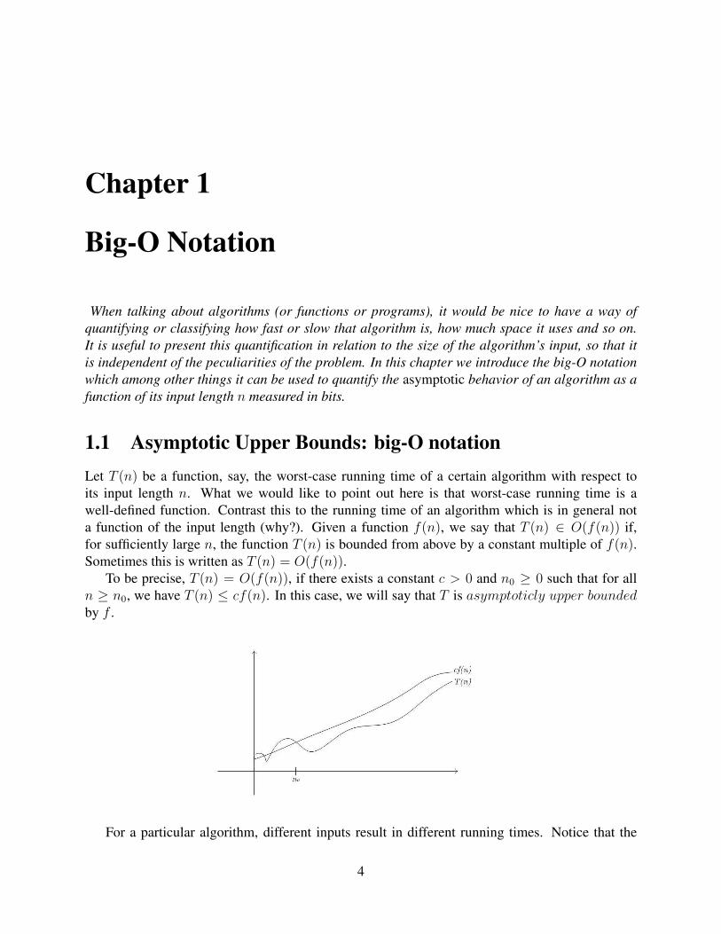
When talking about algorithms (or functions or programs), it would be nice to have a way ofquantifying or classifying how fast or slow that algorithm is, how much space it uses and so on.It is useful to present this quantification in relation to the size of the algorithm’s input, so that itis independent of the peculiarities of the problem. In this chapter we introduce the big-O notationwhich among other things it can be used to quantify the asymptotic behavior of an algorithm as afunction of its input length n measured in bits.
1.1 Asymptotic Upper Bounds: big-O notationLet T (n) be a function, say, the worst-case running time of a certain algorithm with respect toits input length n. What we would like to point out here is that worst-case running time is awell-defined function. Contrast this to the running time of an algorithm which is in general nota function of the input length (why?). Given a function f(n), we say that T (n) ∈ O(f(n)) if,for sufficiently large n, the function T (n) is bounded from above by a constant multiple of f(n).Sometimes this is written as T (n) = O(f(n)).
To be precise, T (n) = O(f(n)), if there exists a constant c > 0 and n0 ≥ 0 such that for alln ≥ n0, we have T (n) ≤ cf(n). In this case, we will say that T is asymptoticly upper boundedby f .
For a particular algorithm, different inputs result in different running times. Notice that the
4
running time of a particular input is a constant, not a function. Running times of interest are thebest, the worst, and the average expressing that the running time is at least, at most and on averagefor each input length n. For us the worst-case execution time is often of particular concern sinceit is important to know how much time might be needed in the worst case to guarantee that thealgorithm will always finish on time. Similarly, for the worst-case space used by an algorithm.From this point on unless stated otherwise the term “running time” is used to refer to “worst-caserunning time”.
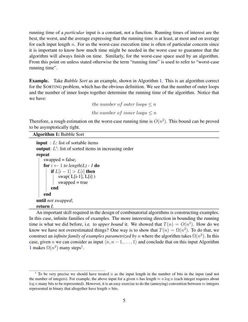
Example. Take Bubble Sort as an example, shown in Algorithm 1. This is an algorithm correctfor the SORTING problem, which has the obvious definition. We see that the number of outer loopsand the number of inner loops together determine the running time of the algorithm. Notice thatwe have:
the number of outer loops ≤ n
the number of inner loops ≤ n
Therefore, a rough estimation on the worst-case running time is O(n2). This bound can be provedto be asymptotically tight.
Algorithm 1: Bubble Sort
input : L: list of sortable itemsoutput: L′: list of sorted items in increasing orderrepeat
swapped = false;for i← 1 to length(L) - 1 do
if L[i− 1] > L[i] thenswap( L[i-1], L[i] )swapped = true
endend
until not swapped;return LAn important skill required in the design of combinatorial algorithms is constructing examples.
In this case, infinite families of examples. The more interesting direction in bounding the runningtime is what we did before, i.e. to upper bound it. We showed that T (n) = O(n2). How do weknow we have not overestimated things? One way is to show that T (n) = Ω(n2). To do that, weconstruct an infinite family of examples parametrized by n where the algorithm takes Ω(n2). In thiscase, given n we can consider as input 〈n, n− 1, . . . , 1〉 and conclude that on this input Algorithm1 makes Ω(n2) many steps1.
1 To be very precise we should have treated n as the input length in the number of bits in the input (and notthe number of integers). For example, the above input for a given n has length ≈ n log n (each integer requires aboutlog n many bits to be represented). However, it is an easy exercise to do the (annoying) convention between m integersrepresented in binary that altogether have length n bits.
5

Chapter 2
Interval Scheduling
In this lecture, we begin by describing what a greedy algorithm is. UNWEIGHTED INTERVAL
SCHEDULING is one problem that can be solved using such an algorithm. We then presentWEIGHTED INTERVAL SCHEDULING, where greedy algorithms don’t seem to work, and we mustemploy a new technique, dynamic programming, which in some sense generalizes the concept of agreedy algorithm.
2.1 Facts about Greedy AlgorithmsMost greedy algorithms make decisions by iterating the following 2 steps.
1. Order the input elements
2. Make an irrevocable decision based on a local optimization.
Here, irrevocable means that once a decision is made about the partially constructed output, it isnever able to be changed. The greedy approach relies on the hope that repeatedly making locallyoptimal choices will lead to a global optimum.
Most greedy algorithms order the input elements just once, and then make decisions one byone afterwards. Kruskal’s algorithm on minimum spanning trees is a well-known algorithm thatuses the greedy approach. More sophisticated algorithms will reorder the elements in every round.For example, Dijkstra’s shortest path algorithm will update and reorder the vertices to choose theone who’s distance to the vertex is minimized.
Greedy algorithms are often the first choice when one tries to solve a problem for two reasons:
1. The greedy concept is simple.
2. In many common cases, a greedy approach leads to an optimal answer.
We present a simple algorithm to demonstrate the greedy approach.
6

2.2 Unweighted Interval SchedulingSuppose we have a set of jobs, each with a given starting and finishing time. However, we arerestricted to only one machine to deal with these jobs, that is, no two jobs can overlap with eachother. The task is to come up with an arrangement or a “scheduling” that finishes the maximumnumber of jobs within a given time interval. The formal definition of the problem can be describedas follows:
Definition 2.2.1 (Intervals and Schedules). Let S be a finite set of intervals. An interval I is apair of two integers, the first smaller than the second; i.e. I = (a, b) ∈ (Z+)2, a < b. We saythat S ′ ⊆ S is a feasible schedule if no two intervals I, I ′ ∈ S overlap with each other. LetI = (a1, b1), I
′ = (a2, b2); overlap means a2 < b1 ≤ b2 or a1 < b2 ≤ b1.
Problem: UNWEIGTHED INTERVAL SCHEDULING
Input: a finite set fo intervals SOutput: a feasible schedule S ′ ⊆ S, such that |S ′| is maximum (the maximum is taken over thesize of all feasible schedules of S).
Figure 2.1 gives an example instance of the Unweighted Interval Scheduling Problem. Hereinterval (1, 7) and interval (6, 10) overlap with each other.
(Failed) attempt 1: Greedy rule: Order the intervals in ascending order by length, then choosethe smaller intervals first. The intuition behind this solution is that shorter jobs may be less likelyto overlap with other jobs. So we order the intervals in ascending order, then we choose jobs whichdo not overlap with the ones we have already chosen (choosing the shortest job which fulfils thisrequirement). However, this solution is not correct.
Figure 2.1: An example of the time line and intervals
Figure 2.2 gives a counterexample in which this greedy rule fails. Giving a counterexample isa standard technique to show that an algorithm is not correct1. In this example, the optimal choiceis job 1 and job 3. But by adhering to a greedy rule that applies to the length of a job, we can onlychoose job 2. Solution 1 gives an answer only 1
2of the optimal. We know that this algorithm is
wrong. But there is still one thing we can ask about this greedy algorithm: How bad can it be? Can1 The definition of a correct algorithm for a given problem, is that for every input (i) the algorithm terminates and
(ii) if it terminates and the input is in the correct form then the output is in the correct form. Therefore, to prove thatan algorithm is not correct for a given problem it is suffcient to show that there exists an input where the output is notcorrect (in this case, by definition of the problem, correct is a schedule of optimal size).
7
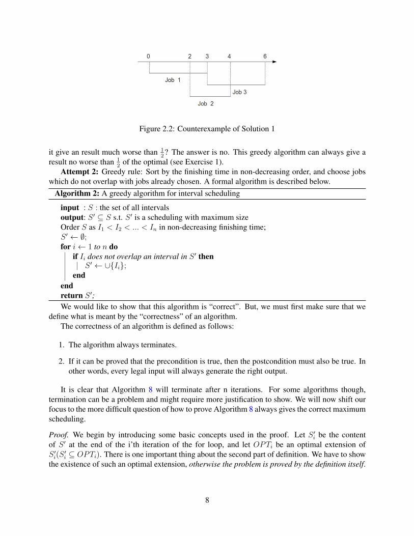
Figure 2.2: Counterexample of Solution 1
it give an result much worse than 12? The answer is no. This greedy algorithm can always give a
result no worse than 12
of the optimal (see Exercise 1).Attempt 2: Greedy rule: Sort by the finishing time in non-decreasing order, and choose jobs
which do not overlap with jobs already chosen. A formal algorithm is described below.Algorithm 2: A greedy algorithm for interval scheduling
input : S : the set of all intervalsoutput: S ′ ⊆ S s.t. S ′ is a scheduling with maximum sizeOrder S as I1 < I2 < ... < In in non-decreasing finishing time;S ′ ← ∅;for i← 1 to n do
if Ii does not overlap an interval in S ′ thenS ′ ← ∪Ii;
endendreturn S ′;We would like to show that this algorithm is “correct”. But, we must first make sure that we
define what is meant by the “correctness” of an algorithm.The correctness of an algorithm is defined as follows:
1. The algorithm always terminates.
2. If it can be proved that the precondition is true, then the postcondition must also be true. Inother words, every legal input will always generate the right output.
It is clear that Algorithm 8 will terminate after n iterations. For some algorithms though,termination can be a problem and might require more justification to show. We will now shift ourfocus to the more difficult question of how to prove Algorithm 8 always gives the correct maximumscheduling.
Proof. We begin by introducing some basic concepts used in the proof. Let S ′i be the contentof S ′ at the end of the i’th iteration of the for loop, and let OPTi be an optimal extension ofS ′i(S
′i ⊆ OPTi). There is one important thing about the second part of definition. We have to show
the existence of such an optimal extension, otherwise the problem is proved by the definition itself.
8
Remark 2.2.2. You may wonder why we are concerned about a different OPTi (one for eachiteration i). This is because after the base case is established, we find OPTn by assuming it hasbeen proved for all values between the base case and OPTn−1, inclusive. This is the way inductionworks.
We will show by induction that
P (i) : ∀i,∃OPTi s.t. S ′i ⊆ OPTi
For the base case, P (0), it is trivial to get S ′0 = ∅ and S ′0 ⊆ OPT0. For the inductive step,suppose we have P (k) and we want to solve P (k + 1). At time k + 1, we consider interval Ik+1:
• Case I: Ik+1 /∈ S ′k+1. We can construct OPTk+1 = OPTk. It is obvious that S ′k+1 = S ′k ⊆OPTk+1.
• Case II: Ik+1 ∈ S ′k+1
– Subcase a: Ik+1 does not overlap OPTk.This case cannot happen since it contradicts with the definition of OPTk.
– Subcase b: Ik+1 overlaps exactly one interval I∗ from OPTk.Since Ik+1 ∈ S ′k+1, Ik+1 will not overlap any interval in S ′k, which implies I∗ ∈ OPTk\S ′k. So S ′k ⊆ OPTk\I∗. Then we can constructOPTk+1 = (OPTk\I∗)∪Ik+1.S ′k+1 = S ′k ∪ Ik+1, where S ′k ⊆ OPTk \ I∗. So S ′k+1 ⊆ OPTk+1.
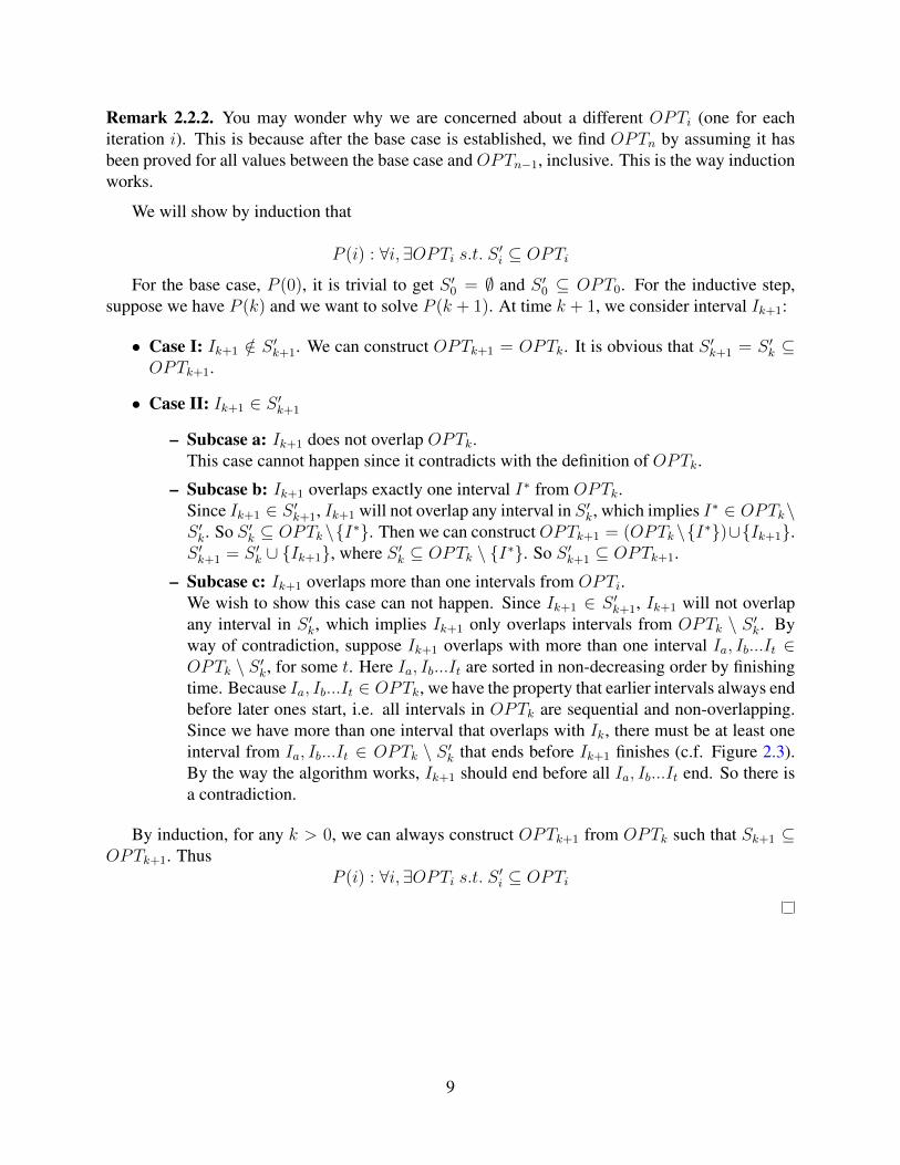
– Subcase c: Ik+1 overlaps more than one intervals from OPTi.We wish to show this case can not happen. Since Ik+1 ∈ S ′k+1, Ik+1 will not overlapany interval in S ′k, which implies Ik+1 only overlaps intervals from OPTk \ S ′k. Byway of contradiction, suppose Ik+1 overlaps with more than one interval Ia, Ib...It ∈OPTk \ S ′k, for some t. Here Ia, Ib...It are sorted in non-decreasing order by finishingtime. Because Ia, Ib...It ∈ OPTk, we have the property that earlier intervals always endbefore later ones start, i.e. all intervals in OPTk are sequential and non-overlapping.Since we have more than one interval that overlaps with Ik, there must be at least oneinterval from Ia, Ib...It ∈ OPTk \ S ′k that ends before Ik+1 finishes (c.f. Figure 2.3).By the way the algorithm works, Ik+1 should end before all Ia, Ib...It end. So there isa contradiction.
By induction, for any k > 0, we can always construct OPTk+1 from OPTk such that Sk+1 ⊆OPTk+1. Thus
P (i) : ∀i,∃OPTi s.t. S ′i ⊆ OPTi
9

Figure 2.3: An example of Case II(b): There are two intervals Ia and Ib from OPTk overlaps withIk
2.3 Weighted Interval SchedulingThis interval scheduling problem is identical to the previous problem, but with the difference thatall intervals are assigned weights; i.e. a weighted interval I can be identified with I = (a, b) andan integer w(I) which is its weight .Input: S : a set of weighted intervals S and w : S → NOutput: A schedule S ′ ⊆ S of maximum total weight.
Figure 2.4: An example of Weighted Interval Scheduling
Unlike the Unweighted Interval Scheduling problem, no natural greedy algorithm is known forsolving its weighted counterpart. It can be solved, however, via a different technique if we breakthe problem into sub-problems: dynamic programming. Now instead of just greedily buildingup one solution, we create a table and in each round we “greedily” compute an optimal solutionto a subproblem by using the values of the optimal solutions of smaller subproblems we haveconstructed before.
Of course, not every problem can be solved via Dynamic Programming (DP). Roughly speak-ing, DP implicitly explores the entire solution space by decomposing the problem into sub-problems,and then using the solutions to those sub-problems to assist in solutions for larger and larger sub-problems.
After ordering intervals in non-decreasing order by finishing time, an example sub-problem inWEIGHTED INTERVAL SCHEDULING is to give the scheduling with maximum total weight up toa specified finishing time. For example, say that the input consists of the intervals I1, I2, I3, I4,and that the finishing time of I1 is the smallest then it’s I2, then I3 and then I4. The DP algo-rithm computes the optimal schedule if the input consists only of I1, then it computes the opti-mal schedule if the input consists of I1, I2, then it computes the optimal schedule if the inputconsists of I1, I2, I3 and finally it computes the optimal schedule if the input consists of theentire list I1, I2, I3, I4. The reader should understand the following: (1) what would have hap-pened if we had defined the subproblems without ordering the intervals in non-decreasing finishingtime order and (2) how do we use the fact that in order to compute the optimal solution to input
10

I1, . . . , Ik we should have recorded in ur table all previous solutions to subproblems defined oninputs I1, . . . , Ik−1, I1, . . . , Ik−2, I1, . . . , Ik−3, . . . .
Algorithm 3: A dynamic programming algorithm for weighted interval scheduling
input : S : the set of all weighted intervalsoutput: S ′ ⊆ S s.t. S ′ is a scheduling of maximum total weightOrder S by I1 < I2 < ... < In in non-decreasing finishing time;S ′ ← ∅;for i← 1 to n do
Let j be the largest integer s.t. S’[j] contains intervals not overlapping Ii;S ′[i]← maxS ′[i− 1], S ′[j] + w[Ii]
endreturn S ′;We will use the example illustrated in Figure 2.4 as the input to Algorithm 3. At the end of
Algorithm 3’s execution, the S ′ array should look like the following:
0 5 11 100 100 150
We remark that unlike greedy algorithms, in Dynamic Programming algorithms the correctnessis transparent in the description of the algorithm. Usually, the difficulty in a DP algorithm is comingup with a recurrence relation which relates optimal solutions of smaller subproblems to bigger ones(this recurrence relation is usually trivial to implement as an algorithm).
Exercise 1. Show why Attempt 1 given for the Unweighted Interval Scheduling problem cannotbe worse than half of the optimal.
11
Chapter 3
Sequence Alignment: can we do DynamicProgramming in small space?
In this course problems come in two forms: search and optimization. For example, the SEARCH
SHORTEST PATH problem is for a given input to find an actual shortest path, whereas the opti-mization version of the problem is to find the value (i.e how long) is such a path. In this chapter, wedefine the SEQUENCE ALIGNMENT problem, and give a dynamic programming algorithm whichsolves it. It is very interesting that there is a conceptual difference in the algorithms that solvethe SEARCH and the OPTIMIZATION version of problems. In particular, although it is easy tofind an optimal Dynamic Programming algorithm for the optimization problem which uses littlespace, it is more involved to come up with a time-efficient algorithm that uses little space for thesearch version of the problem. To that end, we will combine Dynamic Programming and Divideand Conquer and we will give a solution which uses little time and simultaneously little space.
3.1 Sequence Alignment ProblemSequence alignment has a very common every day application: spell check. When we type “Algo-rthsm” when we mean to type “Algorithm”, the computer has to find similar words to the one wetyped and give us suggestions. In this situation, computers have to find the “nearest” word to theone we typed. This begs the question, how can we define the “nearest” word for a sequence? Wewill give a way to score the difference (or similarity) between strings. Apart from spell checkersthis finds application to algorithms on DNA sequences. In fact, such DNA sequences have hugesizes, so an algorithm that works using space n and algorithm that works using space n2 make abig difference in practice!
Usually, alignments add gaps or insert/delete characters in order to make two sequences thesame. Let δ be a gap cost and αa,b be the cost of a mismatch between a and b. We define thedistance between a pair of sequences as the minimal alignment cost.
In the example above we have:
algor thsm
algorith m
12

In the above alignment, we add a total of two gaps to the sequences. We can say that thealignment cost in this case is 2δ. Notice that for any sequence pair, there is more than one way tomake them same. Different alignments may lead to different costs.
For example, the sequence pair: “abbba” and “abaa”, two sequences over the alphabet Σ =a, b. We could assign an alignment cost of δ + αa,b:
abbba
ab aa
Or we could assign an alignment cost of 3δ:
abbba
ab aa
Notice that the relationship between δ and α may lead to different minimal alignments.Now we give a formal description of the Sequence Alignment Problem:
• INPUT: Two sequences X, Y over alphabet Σ.
• OUTPUT: An alignment of minimum cost.
Definition 3.1.1 (Alignment). Let X = x1x2...xn and Y = y1y2...ym. An alignment between Xand Y is a setM ⊆ 1, 2, ..., n×1, 2, ...,m, such that @(i, j), (i′, j′) ∈M , where i ≤ i′, j′ ≤ j.
3.2 Dynamic AlgorithmClaim 3.2.1. Let X, Y be two sequences and M be an alignment. Then one of the following istrue:
1. (n,m) ∈M
2. the nth position of X is unmatched.
3. the mth position of Y is unmatched.
Proof. When we want to make an alignment for sequencesX and Y , for any (n,m) ∈ 1, 2, ..., n×1, 2, ...,m, one of three situations occur: xn and ym form a mismatch, xn should be deleted fromX , or ym should be inserted into X . Notice that inserting a blank into the same position for bothX and Y can never reach a best alignment, so omit this case.
We denote by Opt(i, j) the optimal solution to the subproblem of aligning sequences X i =x1x2...xi and Y j = y1y2...yj . We denote by αxi,yj the mismatch cost between xi and yj and by δthe gap cost. From the claim above, we have:
Opt(i, j) = min
αxi,yj +Opt(i− 1, j − 1),
δ +Opt(i− 1, j)δ +Opt(i, j − 1)
13

We can now present a formal dynamic programming algorithm for Sequence Alignment:Algorithm 4: Sequence-Alignment-Algorithm
input : Two sequences X, Y over alphabet Σoutput: Minimum alignment costfor i← 0 to n do
for j ← 0 to m doif i = 0 or j = 0 then
Opt(i, j) = (i+ j)× δ;endelse
Opt(i, j) = minαxi,yj +Opt(i− 1, j− 1), δ+Opt(i− 1, j), δ+Opt(i, j− 1);end
endendreturn Opt(n,m)
It is clear that the running time and the space cost are both O(nm) (the nxm array Opt(i, j)for space and the nested for loops give us the running time). However, we could improve theAlgorithm 4 by reducing the space required while at the same time not increasing the running time!We can make an algorithm with space O(n+m) using another technique, Divide-And-Conquer.
Remark 3.2.2. In fact, we can compute the value of the optimal alignment easily in space onlyO(m). When computing Opt(k + 1, j), we only need the value of Opt(k, j). Thus we can releasethe space Opt(0, j)...Opt(k − 1, j)∀j = 0...m. We will call this the Space-efficient-Alignment-Algorithm.
3.3 ReductionWe will introduce the Shortest Path on Grids with Diagonals problem and then reduce the SequenceAlignment problem to it. An example of the Shortest Path on Grids with Diagonals problem isgiven in Figure 3.1.
We are given two sequences X = x1x2...xn and Y = y1y2...ym. Let the ith row of a grid (withdiagonals) represent xi in X , and the jth column of a grid represent yj in Y . Let the weight ofevery vertical/horizontal edge be δ and the weight of a diagonal be αxiyj . The shortest path on thisgraph from u to v is the same as the minimum alignment cost of two sequence.
Figure 3.1 gives an example of a grid with diagonals, GXY . x1 is matched to the first column,x2 is matched to the second column. If we move horizontally from left to right on the first rowstarting from u, then this means x1 is matched to a gap. Similarly, y2 is matched to the bottomrow, y1 is matched to the upper row. If we move vertically from bottom to top, this means y1 ismatched to a gap. When we use diagonals, some letter of the two sequence are matched together,for example, if we move along the diagonal closest to u, then x1 is matched to y1. No matter theroute we take (only allowing moves up, right and north-east diagonal), we can always find a pathfrom u to v on GXY . Moreover, this path always corresponds to an alignment of X and Y and viceversa.
14

Figure 3.1: An example of grids with diagonals, GXY
Claim 3.3.1. The minimum value for the Shortest Path on Grids with Diagonals is the same as theminimum value alignment cost for Sequence Alignment.
Proof. (sketch) For any two input sequences, a feasible solution for the Sequence Alignment prob-lem can always have a one to one mapping to a feasible solution for the Shortest Path on Gridswith Diagonals problem.
In the Sequence-Alignment algorithm, if we know the value of the last row, we can run thealgorithm in reverse. We call this algorithm the Reverse-Sequence-Alignment algorithm. Letf [i][j] store the value of the shortest path from u to location (i, j), and g[i][j] store the value ofthe Reverse-Sequence-Alignment algorithm at location (i, j). In other words, g[i][j] is the optimalalignment of subsequences xixi+1...xn and yjyj+1...ym.
Claim 3.3.2. The shortest path in GXY that passes through (i, j) has length f [i][j] + g[i][j].
Proof. Any path that passes through (i, j) can be divided into two shorter paths, one from u to(i, j) and the other from (i, j) to v. The shortest path from u to (i, j) is f [i][j]. Since the weightsalong the edges are fixed in GXY no matter which way they are traversed, the shortest path from(i, j) to v is equal to the value of the shortest path from v to (i, j), which is g[i][j]. So the minimumcost from u to v through (i, j) is f [i][j] + g[i][j].
Claim 3.3.3. For a fixed number q, let k be the number that minimizes f [q][k]+g[q][k]. Then thereexists a shortest path from u to v passing through (q, k).
Proof. Suppose there does not exist a shortest path from u to v passing through (q, k). For a fixednumber q, all the pathes from u to v must pass through some point (q, t), t ∈ 1...m. Thus, ashortest path L must pass through some point (q, k′). According to our assumption, L cannot passthrough (q, k), which means that in particular, f [q][k′] + f [q][k′] < f [q][k] + g[q][k]. This is acontradiction.
15

We give the final algorithm based on the Divide and Conquer technique below:
Algorithm 5: Divide and Conquer Alignment Algorithm(X, Y )
input : Two sequences X = x1x2...xn, Y = y1y2...ynoutput: The node on the u− v shortest path on GXY
if n ≤ 2 or m ≤ 2 thenexhaustively compute the optimal and quit;
endCall Sequence-Alignment algorithm(X, Y [1,m/2])Call Reverse-Sequence-Alignment algorithm(X, Y [m/2 + 1,m])Find q minimize f [q][m/2] + g[q][m/2]Add [q,m/2] to the output.Call Divide-and-Conquer-Algorithm(X[1, q], Y [1,m/2])Call Divide-and-Conquer-Algorithm(X[q, n], Y [m/2 + 1,m])
The space required in Algorithm 5 isO(n+m). This is because we divideGXY along its centercolumn and compute the value of f [i][m/2] and g[i][n/2] for each value of i. Since we apply therecursive calls sequentially and reuse the working space from one call to the next, we end up withspace O(n+m).
We claim the running time of the algorithm is O(nm): Let size = nm, we find that f(size) =O(size) + f( size
2). This is because the first calls to Sequence-Alignment and Reverse-Sequence-
Alignment each need O(size) time, and the latter two calls need f( size2
) time. Solving the recur-rence, we have the running time is O(nm).
16
Chapter 4
Matchings and Flows
In this chapter, we discuss matchings and flows from a combinatorial perspective. In a subsequentlecture we will discuss the same issues using Linear Programming. We introduce the problem ofmaximum flow, and algorithms for solving solve it, including the Ford-Fulkerson method and onepolynomial time instantiation of it, the Edmonds-Karp algorithm. We prove the maximum flow -minimum cut theorem, and we show the polynomial time bound for Edmonds-Karp. Then, we applynetwork flows to solve the maximum bipartite matching problem. Finally, we apply non-bipartitematchings to give a 2-approximation algorithm for Vertex Cover.
4.1 IntroductionMatching and flow are basic concepts in graph theory. And they have many applications in practice.Basically , in a graph a matching is a set of edges of which any two edges does not share a commonend node. And a network flow in a directed weighed graph is like a distribution of workloadsaccording to the capacity of each edge.
In this lecture,we are going to talk about maximum bipartite matchings. Formally, we have thefollowing definitions :
Definition 4.1.1 (Bipartite Matching). For a graph G = (X, Y,E),we say that M ⊆ E is a (bipar-tite) matching if every vertex u ∈ (X ∪ Y ) appears at most once in M.
Now we are aware of the formal definition of a matching, we can introduce the main problemwe are gonna talk about today and the day following – Maximum Matching Problem.
Definition 4.1.2 (Maximum Matching). In a bipartite graphG = (X, Y,E),M ⊆ E is a matching.Then M is a maximum matching if for every matching M ′ in G, |M ′| ≤ |M |. j.
Definition 4.1.3 (Maximal Matching). In a bipartite graph G = (X, Y,E), M ⊆ E is a matching.Then M is a maximal matching if there does not exist a matching M ′ ⊃M .
Remark 4.1.4. Notice that we use the term “maximum” and not “maximal”. These two are differ-ent. A “maximal” matching is a matching that we can not add more edges into and keep it still amatching; while a “maximum” matching is the maximal matching with largest size. Here we givean example in Figure 4.1.
17

Figure 4.1: This figure shows the difference between a maximum matching and a maximal matching.
Here we define the Maximum Bipartite Matching problem.
Definition 4.1.5. Maximum Bipartite Matching
• Input: A bipartite graph G = (X, Y,E).
• Output: A maximum matching M ⊆ E.
The maximum bipartite matching problem is fundamental in graph theory and theoretical com-puter science. It can be solved in polynomial time. BUT notice that there exists NO dynamicprogramming algorithm that can solve this problem. In order to solve this problem, we introduceanother problem called the Maximum Flow Problem. Later we’ll see how can we solve maximummatching using maximum flow.
4.2 Maximum Flow ProblemWhat is a FLOW? The word ”flow” reminds us of water flow in a first impression. Yes, networkflow is just like pushing water from the source to the sink, with the limitation of the capacity ofeach pipe(here it’s edge in a graph). And a maximum flow problem is just pushing as much waterin as we can. Formally the definition of a network flow is as follows:
Definition 4.2.1 (Network Flow). Given (G, s, t, c), where G is a graph (V,E),s, t ∈ V ,c is afunction which maps an edge to a value, a flow f : E → R is a function where :
1. f(e) ≤ c(e),∀e ∈ E
2.∑∀e=(u,v) f(e) =
∑∀e′=(v,w) f(e
′),∀v ∈ V
We define the value of a flow v(f) as v(f) =∑∀e=(s,u) f(e), which means the sum of all the
edges leading out of the source s. And the maximum flow problem is defined as follows:
Definition 4.2.2. Maximum Flow Problem
• Input: (G,s,t,c).
• Output: a flow in the graph with maximum value.
18
•s3/2 // •u
2/2 // •t *4 •s 1 // •u2
ii •t2oo
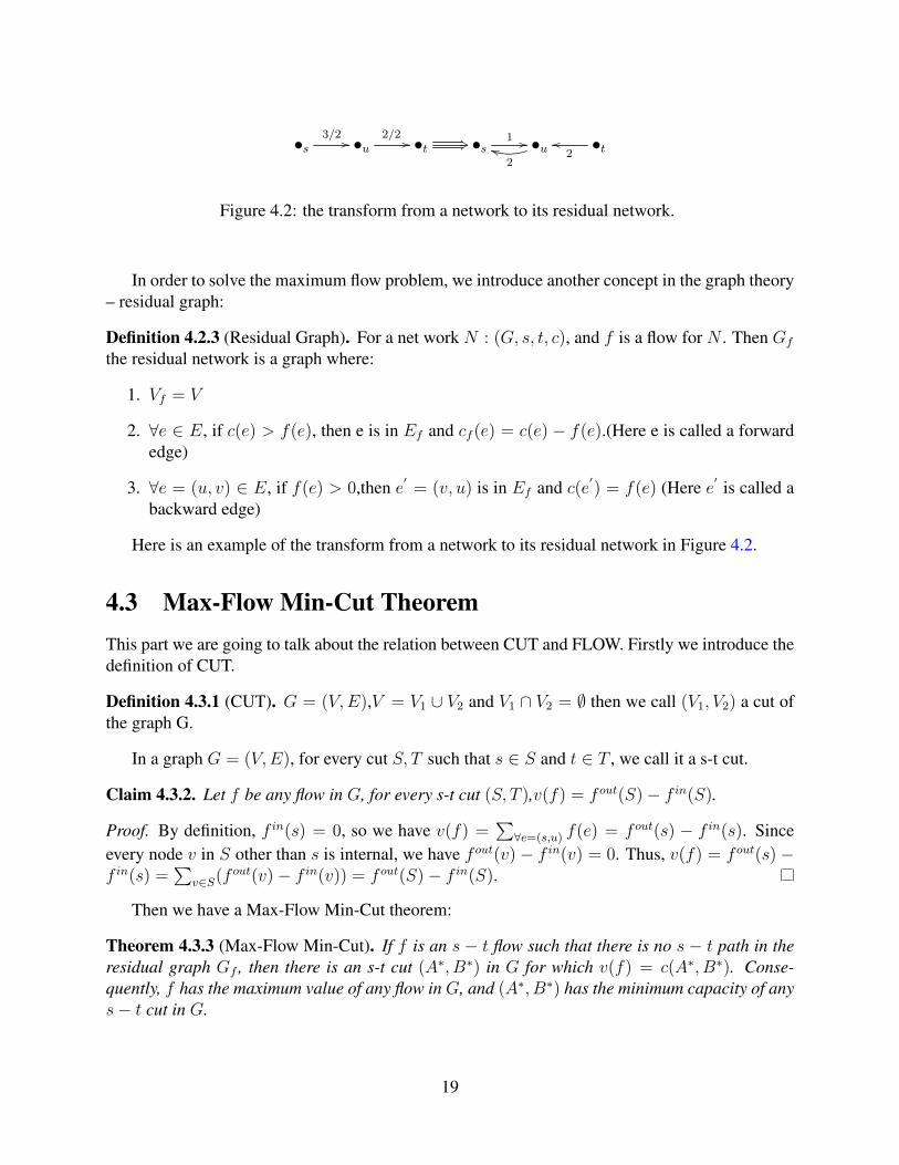
Figure 4.2: the transform from a network to its residual network.
In order to solve the maximum flow problem, we introduce another concept in the graph theory– residual graph:
Definition 4.2.3 (Residual Graph). For a net work N : (G, s, t, c), and f is a flow for N . Then Gf
the residual network is a graph where:
1. Vf = V
2. ∀e ∈ E, if c(e) > f(e), then e is in Ef and cf (e) = c(e)− f(e).(Here e is called a forwardedge)
3. ∀e = (u, v) ∈ E, if f(e) > 0,then e′ = (v, u) is in Ef and c(e′) = f(e) (Here e′ is called abackward edge)
Here is an example of the transform from a network to its residual network in Figure 4.2.
4.3 Max-Flow Min-Cut TheoremThis part we are going to talk about the relation between CUT and FLOW. Firstly we introduce thedefinition of CUT.
Definition 4.3.1 (CUT). G = (V,E),V = V1 ∪ V2 and V1 ∩ V2 = ∅ then we call (V1, V2) a cut ofthe graph G.
In a graph G = (V,E), for every cut S, T such that s ∈ S and t ∈ T , we call it a s-t cut.
Claim 4.3.2. Let f be any flow in G, for every s-t cut (S, T ),v(f) = f out(S)− f in(S).
Proof. By definition, f in(s) = 0, so we have v(f) =∑∀e=(s,u) f(e) = f out(s) − f in(s). Since
every node v in S other than s is internal, we have f out(v)− f in(v) = 0. Thus, v(f) = f out(s)−f in(s) =
∑v∈S(f out(v)− f in(v)) = f out(S)− f in(S).
Then we have a Max-Flow Min-Cut theorem:
Theorem 4.3.3 (Max-Flow Min-Cut). If f is an s − t flow such that there is no s − t path in theresidual graph Gf , then there is an s-t cut (A∗, B∗) in G for which v(f) = c(A∗, B∗). Conse-quently, f has the maximum value of any flow in G, and (A∗, B∗) has the minimum capacity of anys− t cut in G.
19
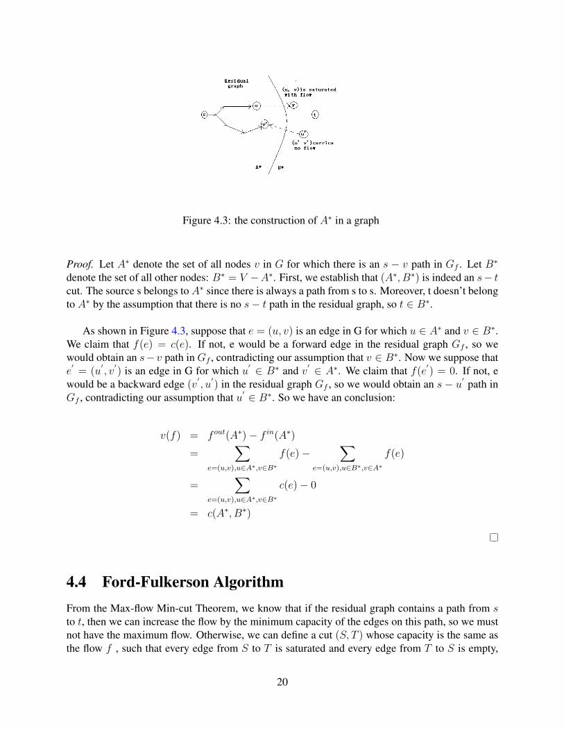
Figure 4.3: the construction of A∗ in a graph
Proof. Let A∗ denote the set of all nodes v in G for which there is an s − v path in Gf . Let B∗
denote the set of all other nodes: B∗ = V −A∗. First, we establish that (A∗, B∗) is indeed an s− tcut. The source s belongs to A∗ since there is always a path from s to s. Moreover, t doesn’t belongto A∗ by the assumption that there is no s− t path in the residual graph, so t ∈ B∗.
As shown in Figure 4.3, suppose that e = (u, v) is an edge in G for which u ∈ A∗ and v ∈ B∗.We claim that f(e) = c(e). If not, e would be a forward edge in the residual graph Gf , so wewould obtain an s− v path in Gf , contradicting our assumption that v ∈ B∗. Now we suppose thate′
= (u′, v′) is an edge in G for which u′ ∈ B∗ and v′ ∈ A∗. We claim that f(e
′) = 0. If not, e
would be a backward edge (v′, u′) in the residual graph Gf , so we would obtain an s− u′ path in
Gf , contradicting our assumption that u′ ∈ B∗. So we have an conclusion:
v(f) = f out(A∗)− f in(A∗)
=∑
e=(u,v),u∈A∗,v∈B∗f(e)−
∑e=(u,v),u∈B∗,v∈A∗
f(e)
=∑
e=(u,v),u∈A∗,v∈B∗c(e)− 0
= c(A∗, B∗)
4.4 Ford-Fulkerson AlgorithmFrom the Max-flow Min-cut Theorem, we know that if the residual graph contains a path from sto t, then we can increase the flow by the minimum capacity of the edges on this path, so we mustnot have the maximum flow. Otherwise, we can define a cut (S, T ) whose capacity is the same asthe flow f , such that every edge from S to T is saturated and every edge from T to S is empty,
20
which implies that f is a maximum flow and (S, T ) is a minimum cut. Based on the theorem, wecan have the Ford-Fulkerson Algorithm: Starting with the zero flow, repeatedly augment the flowalong any path s-t in the residual graph, until there is no such path.
Algorithm 6: Ford-Fulkerson Algorithm
input : A network (G,s,t,c)output: a flow in the graph with maximum value∀e, f(e)← 0while ∃s− t path do
f′ ← augment(f, p)f ← f
′
Gf ← Gf ′
endreturn fNotice that the augment(f, p) in the algorithm.This is an updating procedure of the graph.It
means to find randomly a s− t path and push through a flow of minimum capacity of this path.Also there are several things we need to know about the Ford-Fulkerson Algorithm:
1. Ford-Fulkerson Algorithm does not always terminate when we have real numbers assign-ment. Consider the flow network shown in Figure 4.4, with source s, sink t,capacities ofedges e1,e2 and e3 respectively 1, r =
√5−12
and the capacity of all other edges some integerM ≥ 2. Here the constant r was chosen so r2 = 1−r. We use augmenting paths according tothe table, where p1 = s, v4, v3, v2, v1, t,p2 = s, v2, v3, v4, t,p3 = s, v1, v2, v3, t. Notethat after step 1 as well as after step 5, the residual capacities of edges e1, e2 and e3 are in theform rn, rn+1 and 0, respectively, for some n ∈ N. This means that we can use augment-ing paths p1, p2, p1 and p3 infinitely many times and residual capacities of these edges willalways be in the same form. Total flow in the network after step 5 is 1+2(r1+r2). If we con-tinue to use augmenting paths as above, the total flow converges to 1+2
∑i=1 infri = 3+2r
, while the maximum flow is 2M + 1. In this case, the algorithm never terminates and theflow doesn’t even converge to the maximum flow.
2. if function c maps the edges to integer, then FF outputs integer value.
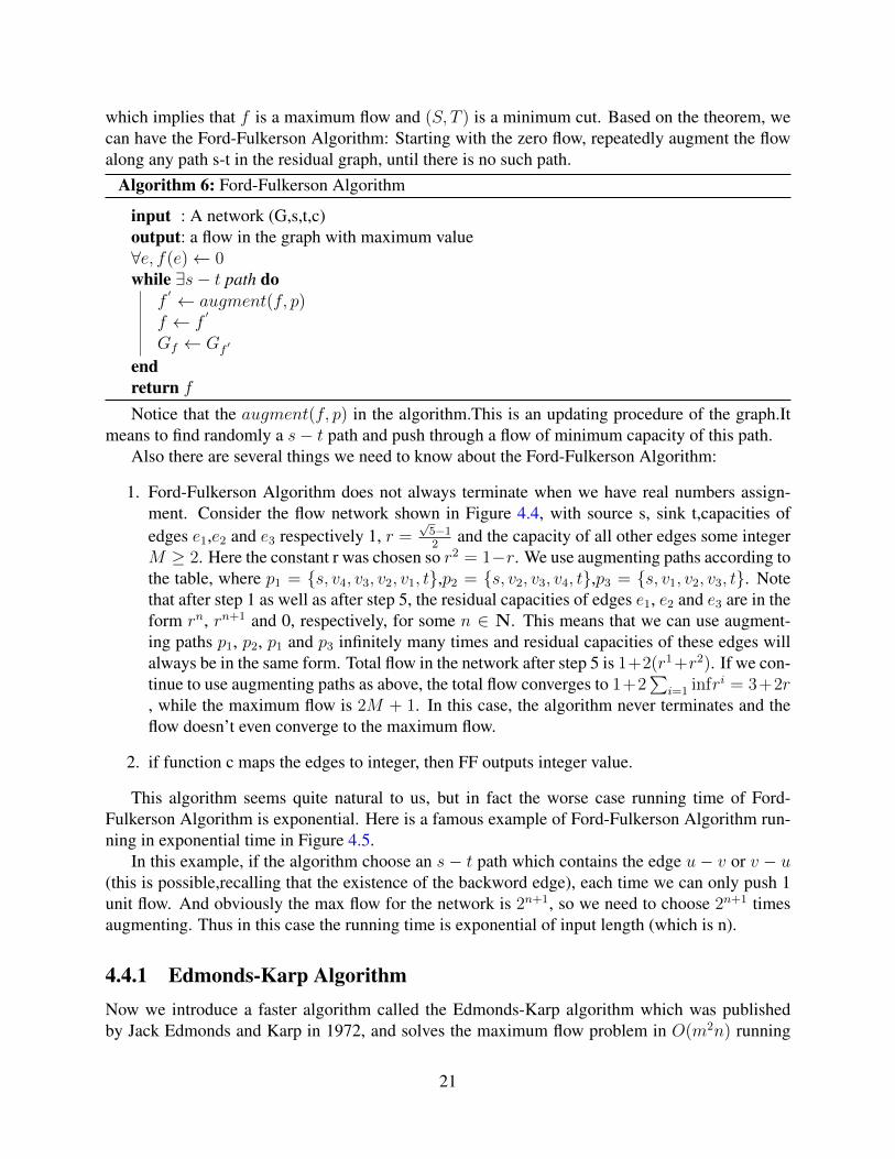
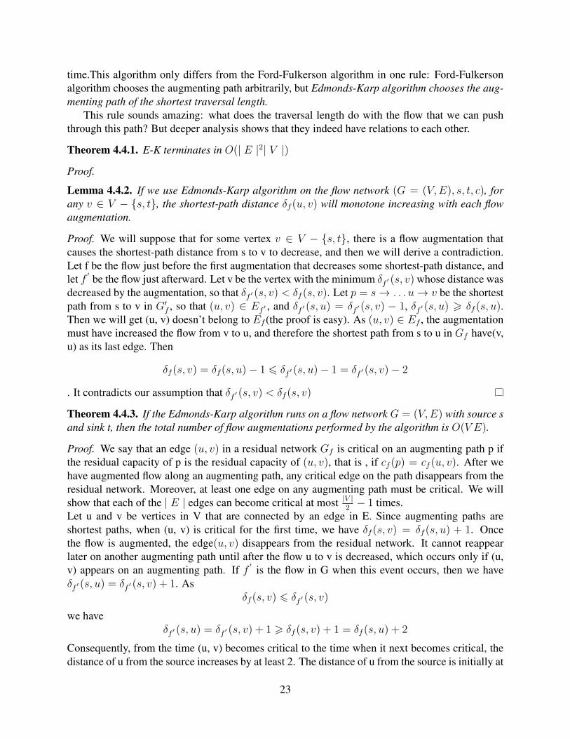
This algorithm seems quite natural to us, but in fact the worse case running time of Ford-Fulkerson Algorithm is exponential. Here is a famous example of Ford-Fulkerson Algorithm run-ning in exponential time in Figure 4.5.
In this example, if the algorithm choose an s− t path which contains the edge u− v or v − u(this is possible,recalling that the existence of the backword edge), each time we can only push 1unit flow. And obviously the max flow for the network is 2n+1, so we need to choose 2n+1 timesaugmenting. Thus in this case the running time is exponential of input length (which is n).
4.4.1 Edmonds-Karp AlgorithmNow we introduce a faster algorithm called the Edmonds-Karp algorithm which was publishedby Jack Edmonds and Karp in 1972, and solves the maximum flow problem in O(m2n) running
21
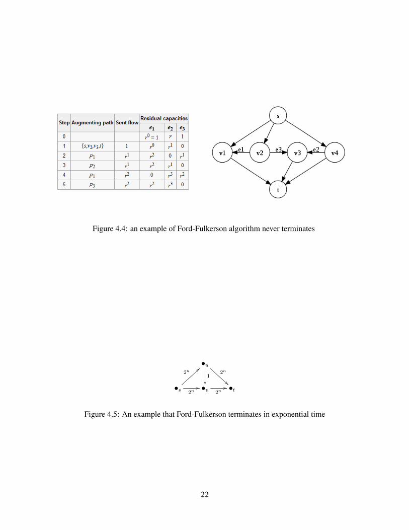
Figure 4.4: an example of Ford-Fulkerson algorithm never terminates
•u2n
1
•s
2n>>
2n// •v 2n
// •t
Figure 4.5: An example that Ford-Fulkerson terminates in exponential time
22
time.This algorithm only differs from the Ford-Fulkerson algorithm in one rule: Ford-Fulkersonalgorithm chooses the augmenting path arbitrarily, but Edmonds-Karp algorithm chooses the aug-menting path of the shortest traversal length.
This rule sounds amazing: what does the traversal length do with the flow that we can pushthrough this path? But deeper analysis shows that they indeed have relations to each other.
Theorem 4.4.1. E-K terminates in O(| E |2| V |)
Proof.
Lemma 4.4.2. If we use Edmonds-Karp algorithm on the flow network (G = (V,E), s, t, c), forany v ∈ V − s, t, the shortest-path distance δf (u, v) will monotone increasing with each flowaugmentation.
Proof. We will suppose that for some vertex v ∈ V − s, t, there is a flow augmentation thatcauses the shortest-path distance from s to v to decrease, and then we will derive a contradiction.Let f be the flow just before the first augmentation that decreases some shortest-path distance, andlet f ′ be the flow just afterward. Let v be the vertex with the minimum δf ′ (s, v) whose distance wasdecreased by the augmentation, so that δf ′ (s, v) < δf (s, v). Let p = s→ . . . u→ v be the shortestpath from s to v in G′f , so that (u, v) ∈ Ef ′ , and δf ′ (s, u) = δf ′ (s, v) − 1, δf ′ (s, u) > δf (s, u).Then we will get (u, v) doesn’t belong to Ef (the proof is easy). As (u, v) ∈ Ef , the augmentationmust have increased the flow from v to u, and therefore the shortest path from s to u in Gf have(v,u) as its last edge. Then
δf (s, v) = δf (s, u)− 1 6 δf ′ (s, u)− 1 = δf ′ (s, v)− 2
. It contradicts our assumption that δf ′ (s, v) < δf (s, v)
Theorem 4.4.3. If the Edmonds-Karp algorithm runs on a flow network G = (V,E) with source sand sink t, then the total number of flow augmentations performed by the algorithm is O(V E).
Proof. We say that an edge (u, v) in a residual network Gf is critical on an augmenting path p ifthe residual capacity of p is the residual capacity of (u, v), that is , if cf (p) = cf (u, v). After wehave augmented flow along an augmenting path, any critical edge on the path disappears from theresidual network. Moreover, at least one edge on any augmenting path must be critical. We willshow that each of the | E | edges can become critical at most |V |
2− 1 times.
Let u and v be vertices in V that are connected by an edge in E. Since augmenting paths areshortest paths, when (u, v) is critical for the first time, we have δf (s, v) = δf (s, u) + 1. Oncethe flow is augmented, the edge(u, v) disappears from the residual network. It cannot reappearlater on another augmenting path until after the flow u to v is decreased, which occurs only if (u,v) appears on an augmenting path. If f ′ is the flow in G when this event occurs, then we haveδf ′ (s, u) = δf ′ (s, v) + 1. As
δf (s, v) 6 δf ′ (s, v)
we haveδf ′ (s, u) = δf ′ (s, v) + 1 > δf (s, v) + 1 = δf (s, u) + 2
Consequently, from the time (u, v) becomes critical to the time when it next becomes critical, thedistance of u from the source increases by at least 2. The distance of u from the source is initially at
23
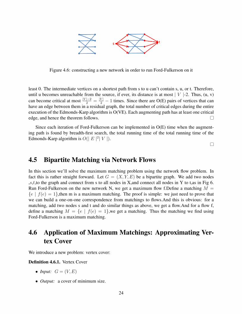
Figure 4.6: constructing a new network in order to run Ford-Fulkerson on it
least 0. The intermediate vertices on a shortest path from s to u can’t contain s, u, or t. Therefore,until u becomes unreachable from the source, if ever, its distance is at most | V |-2. Thus, (u, v)can become critical at most |V |−2
2= |V |
2− 1 times. Since there are O(E) pairs of vertices that can
have an edge between them in a residual graph, the total number of critical edges during the entireexecution of the Edmonds-Karp algorithm is O(VE). Each augmenting path has at least one criticaledge, and hence the theorem follows.
Since each iteration of Ford-Fulkerson can be implemented in O(E) time when the augment-ing path is found by breadth-first search, the total running time of the total running time of theEdmonds-Karp algorithm is O(| E |2| V |).
4.5 Bipartite Matching via Network FlowsIn this section we’ll solve the maximum matching problem using the network flow problem. Infact this is rather straight forward. Let G = (X, Y,E) be a bipartite graph. We add two nodes,s,t,to the graph and connect from s to all nodes in X,and connect all nodes in Y to t,as in Fig 6.Run Ford-Fulkerson on the new network N, we get a maximum flow f.Define a matching M =e | f(e) = 1,then m is a maximum matching. The proof is simple: we just need to prove thatwe can build a one-on-one correspondence from matchings to flows.And this is obvious: for amatching, add two nodes s and t and do similar things as above, we get a flow.And for a flow f,define a matching M = e | f(e) = 1,we get a matching. Thus the matching we find usingFord-Fulkerson is a maximum matching.
4.6 Application of Maximum Matchings: Approximating Ver-tex Cover
We introduce a new problem: vertex cover:
Definition 4.6.1. Vertex Cover
• Input: G = (V,E)
• Output: a cover of minimum size.
24

Here is the definition for COVER:
Definition 4.6.2. Cover : G = (V,E),U ∈ V is a cover if ∀e ∈ E,∃u ∈ U which is a end nodeof e.
Despite the long time of research, the problem remains open.
1. Negative: VC can not be approximated with a factor smaller than 1.363, unless P = NP .’
2. Positive : We have a polynomial algorithm for VC with approximation ratio 2−Ω( 1√log(n)
).
3. Belief : VC cannot be approximated within 2− ε, ∀ε > 0. Notice: in fact under somethingwhich is called the Unique Game Conjecture this is true.
Here is a simple algorithm that approximates VC with ratio 2:
1. compute the maximum matching M in the graph.
2. output the vertices of M.
Proof. Observe that | M |≤ OPT ,where M is the max matching. Also notice that vertices in Mcover G. Suppose that there is a node u which is not covered by M, then it must be connected to anode outside M,say v.Then (u, v) is an edge that does not belong to M,which contradicts that M isa max matching.And the algorithm outputs 2 |M | nodes, and 2 |M |≤ 2OPT
25
Chapter 5
Optimization Problems, Online andApproximation Algorithms
In this chapter, we begin by introducing the definition of an optimization problem followed bythe definition of an approximation algorithm. We then present the Makespan problem as a simpleexample of when an approximation algorithm is useful. Because the Makespan problem is NP-hard, there does not exist a polynomial algorithm to solve it unless P = NP . If we can notfind an exact answer to an arbitrary instance of Makespan in polynomial time, then perhaps wecan give an approximate solution. To this end, we formulate an approximation algorithm for theMakespan problem: Greedy-Makespan. We go on to improve this algorithm to one with a lowerapproximation ratio (i.e. an algorithm that is guaranteed to give an even closer approximation toan optimal answer).
5.1 Optimization ProblemsDefinition 5.1.1. An optimization problem is finding an optimal (best) solution from a set of fea-sible solutions.
Formally, an optimization problem Π consists of:
1. A set of inputs, or instances, I.
2. A set f(I) of feasible solutions, for each given instance I ∈ I.
3. An optimization objective function: c : F → R where F =⋃I∈I f(I). That is, given an
instance I and a feasible solution y, the objective function denotes a “measure” of y with areal number.
The goal of an optimization problem Π is to either give a minimum or maximum: the shortest orlongest path on a graph, for example. For maximization problems, the goal of problem Π is to findan output ∀I , O ∈ f(I), s.t. c(O) = maxO′∈f(I) c(O
′).
For example, in the Unweighted Interval Scheduling Problem, we have 4 intervals, as shownin the following Figure 5.1
26

Here feasible solutions are I1, I2, I1, I2, I3, I4, and I1, I2 is optimal, as it maxi-mizes the number of intervals that can be scheduled.
Notice: In the following section, we will only discuss maximization problems for brevity;minimization problems are in no way fundamentally different.
5.2 Approximation AlgorithmsSometimes we may not know the optimal solution for the problem, if there is no known efficientalgorithm to produce it, for example. In these cases, it might be useful to find an answer thatis “close” to optimal. Approximation algorithms do exactly this, and we present them formallypresently.
Definition 5.2.1 (Approximation Algorithm). Let Π be an optimization problem and A be a poly-nomial time algorithm for Π. For all instances I , denote by OPT (I) the value of the optimal solu-tion, and byA(I) the solution computed byA, for that instance. We say thatA is a c-approximationalgorithm for Π if
∀I, OPT (I) ≤ cA(I)
5.3 Makespan ProblemIn this section, we will discuss the Makespan problem followed by an approximation algorithmwhich solves it. Makespan is a basic problem in scheduling theory: how to schedule a set of jobson a set of machines.
Definition 5.3.1 (Makespan Problem). We are given n jobs with different processing times, t1, t2, ..., tn.The goal is to design a assignment of the jobs to m separate, but identical machines such that thelast finishing time for given jobs (also called makespan) is minimized.
We firstly introduce some basic notations to analysis the Makespan Problem. m ∈ N andt1, t2, ..., tn are given as input. Here, m is the number of machines and t1, t2, ..., tn are the process-ing length of jobs. Figure 5.3 gives an example input. We define Ai to be the set jobs assignedto machine i and Ti to be the total processing time for machine i: Ti =
∑t∈Ai
t. The goal of theproblem is to find a scheduling of the jobs that minimize maxiTi.
Suppose we are given as input: m = 2 ,< t1, t2, t3, t4, t5 >=< 1, 1, 1, 1, 4 >.Of these two possible solutions, the left one is better, in fact it is optimal.
Fact 5.3.2. MAKESPAN is NP-hard.
27
Thus, a polynomial time algorithm to solve an arbitrary instance of Makespan does not existunless P = NP . However, we can find an approximation algorithm that gives a good, albeit pos-sibly suboptimal, solution that can run in polynomial time.
5.4 Approximation Algorithm for Makespan ProblemA greedy approach is often one of the first ideas to try, as it is so intuitive. The basic idea is asfollows: we schedule the jobs from 1 to n, assigning the ith job to the machine with the shortesttotal processing time.
Algorithm 7: Greedy Makespan
input : m ∈ N: number of machines and t1, t2, ..., tn: the processing length of jobsoutput: T : the last finishing time for the schedulingfor i← 1 to n do
choose the smallest T [k] over T [i](i = 1, 2, ...,m)A[k] = A[k] + T [i]T [k] = T [k] + t[i]
endT = mini∈[n]T [i]return T
Theorem 5.4.1. Greedy Makespan is a 2-approximation algorithm for Makespan
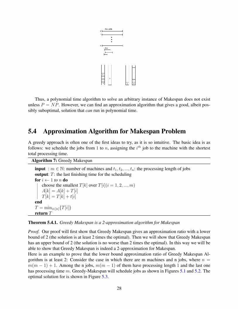
Proof. Our proof will first show that Greedy Makespan gives an approximation ratio with a lowerbound of 2 (the solution is at least 2 times the optimal). Then we will show that Greedy Makespanhas an upper bound of 2 (the solution is no worse than 2 times the optimal). In this way we will beable to show that Greedy Makespan is indeed a 2-approximation for Makespan.Here is an example to prove that the lower bound approximation ratio of Greedy Makespan Al-gorithm is at least 2: Consider the case in which there are m machines and n jobs, where n =m(m − 1) + 1. Among the n jobs, m(m − 1) of them have processing length 1 and the last onehas processing time m. Greedy-Makespan will schedule jobs as shown in Figures 5.1 and 5.2. Theoptimal solution for is shown in Figure 5.3.
28

Figure 5.1: Before placing the last job.
Figure 5.2: After placing the last job
Now we have an approximation ration of Greedy Makespan = 2m−1m
= 2− 1m
. Thus, by exam-ple, we have shown that Greedy Makespan has an approximation ratio lower bound of 2.
We now show that the output of the greedy algorithm is at most twice that of the optimalsolution, i.e. has an upper bound of 2. Firstly we bring in two conspicuously tenable facts:
1. 1m
∑ti ≤ OPT (I).
2. tmax ≤ OPT (I) where tmax is the most wasteful job.
Let T ′k = Tk − tj where tj is the last job assigned to machine k. It is easy to see that T ′k is atmost the average process time. From property (1), we have: T ′k ≤ 1
m
∑i ti ≤ OPT . From property
(2) we have: T ′k = Tk − tj ≥ Tk −OPT . Combining these facts, we get: Tk −OPT ≤ OPT . SoTk ≤ 2OPT .
Now we have an 2-approximation algorithm for Makespan Problem. But can we do better?The answer is yes. Next we will improve this bound with Improved Greedy Makespan.
The only difference between the Improved Greedy Makespan and Greedy Makespan is that theimproved algorithm first sorts ti by non-increasing length before scheduling.
Theorem 5.4.2. Improved Greedy Makespan is a 32-approximation algorithm for Makespan.
Figure 5.3: Optimal solution
29

Proof. Since processing time are sorted in non-increasing order at the beginning of the algorithm,we have t1 ≥ t2 ≥ ... ≥ tn.
In this proof we will make use of the following claim:
Claim 5.4.3. When n ≤ m, Improved Greedy Makespan will obtain an optimal solution. Whenn > m, we have OPT ≥ 2tm+1.
Proof. When n ≤ m, every job is assigned to unique machine, thus the output of the algorithm isequal to the finishing time of the largest job. This is obviously optimal.
When n > m, then by the pigeonhole principle there must be two jobs ti, tj that, in the optimalcase, are assigned to the same machine where i, j ≤ m + 1 and ti, tj ≥ tm+1. We conclude thatOPT ≥ 2tm+1.
When we define: T ′k = Tk − tj , tj the last job assigned to machine k, then we have:
1. If tj is such that j ≤ m, then there is only one job scheduled on machine k. This means thatTk ≤ t1 ≤ OPT .
2. If tj is such that j > m, then machine k should be the one with the shortest total lengthbefore scheduling the jth job. This implies T ′k ≤ 1
j−1∑
i ti ≤1m
∑i ti ≤ OPT .
Furthermore, we have T ′k = Tk − tj ≥ Tk − 12OPT . Thus, Tk − 1
2OPT ≤ OPT , which
implies Tk ≤ 32OPT
So for every k ∈ [m], Tk ≤ 32OPT . Therefore 3
2is an upper bound on the approximation ratio
of Improved Greedy Makespan.
Although we have shown that Improved Greedy Makespan has an approximation ratio of 32,
this bound is not tight. That is, we can do better.
Remark 5.4.4. Improved Greedy Makespan is in fact a 43-approximation algorithm. (Proof omit-
ted)
30
Chapter 6
Introduction to Convex Polytopes
In this lecture, we cover some basic material on the structure of polytopes and linear programming.
6.1 Linear SpaceDefinition 6.1.1 (Linear space). V is a linear space, if V ⊆ Rd, d ∈ Z+, V = span ~u1, ~u2, . . . , ~uk,ui ∈Rd. Equally, we can define linear space as V = ~u|∀c1, c2, . . . , ck ∈ R, ~u = c1 ~u1 + · · ·+ ck ~uk.
Definition 6.1.2 (Dimension). Let dim(V ) be the dimension of a linear space V . The dimensionof a linear space V is the cardinality of a basis of V . A basis is a set of linearly independent vectorsthat, in a linear combination, can represent every vector in a given linear space.
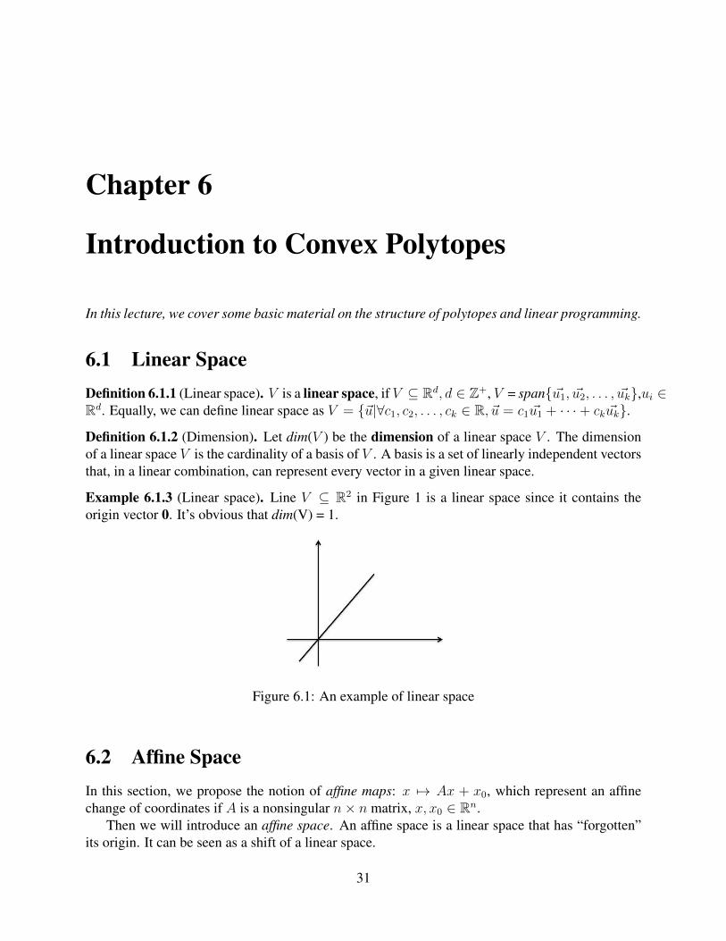
Example 6.1.3 (Linear space). Line V ⊆ R2 in Figure 1 is a linear space since it contains theorigin vector 0. It’s obvious that dim(V) = 1.
Figure 6.1: An example of linear space
6.2 Affine SpaceIn this section, we propose the notion of affine maps: x 7→ Ax + x0, which represent an affinechange of coordinates if A is a nonsingular n× n matrix, x, x0 ∈ Rn.
Then we will introduce an affine space. An affine space is a linear space that has “forgotten”its origin. It can be seen as a shift of a linear space.
31
Definition 6.2.1 (Affine Space). Let V be a linear space. V ′ is an affine space if V ′ = V + ~β,where vector ~v′ ∈ V ′ if and only if ∀~v′ ∈ V ′, ~v′ = ~v + ~β, where ~v is a vector in a linear space V ,and ~β is a fixed scalar for an affine space.
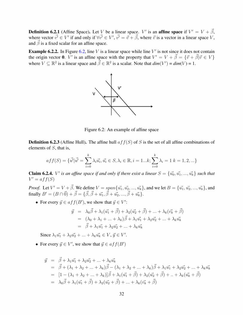
Example 6.2.2. In Figure 6.2, line V is a linear space while line V ′ is not since it does not containthe origin vector 0. V ′ is an affine space with the property that V ′ = V + ~β = ~v + ~β|~v ∈ V where V ⊆ R2 is a linear space and ~β ∈ R2 is a scalar. Note that dim(V ′) = dim(V ) = 1.
Figure 6.2: An example of affine space
Definition 6.2.3 (Affine Hull). The affine hull aff(S) of S is the set of all affine combinations ofelements of S, that is,
aff(S) = ~u′|~u′ =k∑i=0
λi~ui, ~ui ∈ S, λi ∈ R, i = 1...k;k∑i=0
λi = 1 k = 1, 2, ...
Claim 6.2.4. V ′ is an affine space if and only if there exist a linear S = ~u0, ~u1, ..., ~uk such thatV ′ = aff(S)
Proof. Let V ′ = V + ~β. We define V = span ~u1, ~u2, ..., ~uk, and we let B = ~u1, ~u2, ..., ~uk, andfinally B′ = (B ∩~0) + ~β = ~β, ~β + ~u1, ~β + ~u2, ..., ~β + ~uk.
• For every ~y ∈ aff(B′), we show that ~y ∈ V ′:
~y = λ0~β + λ1( ~u1 + ~β) + λ2( ~u2 + ~β) + ...+ λk(~vk + ~β)
= (λ0 + λ1 + ...+ λk)~β + λ1 ~u1 + λ2 ~u2 + ...+ λk ~uk
= ~β + λ1 ~u1 + λ2 ~u2 + ...+ λk ~uk
Since λ1 ~u1 + λ2 ~u2 + ...+ λk ~uk ∈ V , ~y ∈ V ′.
• For every ~y ∈ V ′, we show that ~y ∈ aff(B′)
~y = ~β + λ1 ~u1 + λ2 ~u2 + ...+ λk ~uk
= ~β + (λ1 + λ2 + ...+ λk)~β − (λ1 + λ2 + ...+ λk)~β + λ1 ~u1 + λ2 ~u2 + ...+ λk ~uk
= [1− (λ1 + λ2 + ...+ λk)]~β + λ1( ~u1 + ~β) + λ2( ~u2 + ~β) + ..+ λk( ~uk + ~β)
= λ0~β + λ1( ~u1 + ~β) + λ2( ~u2 + ~β) + ...+ λk(~vk + ~β)
32

So ~y ∈ aff(B′)
6.3 Convex PolytopeDefinition 6.3.1 (Convex body). A Convex bodyK can be defined as: for any two points ~x, ~y ∈ Kwhere K ⊆ Rd, K also contains the straight line segment [~x, ~y] = λ~x+ (1− λ)~y|0 ≤ λ ≤ 1, or[~x, ~y] ⊆ K.
Example 6.3.2. The graph in Figure 6.3(a) is a convex body since for any ~x, ~y ∈ K, [~x, ~y] ⊆ K.However, the graph in Figure 6.3(b) is not a convex body since there exists an ~x, ~y ∈ K ′ such that[~x, ~y] 6⊆ K ′.
(a) (b)
Figure 6.3: (a) An example of convex body (b) An example of non-convex body
Definition 6.3.3 (Convex Hull). For any K ⊆ Rd, the “smallest” convex set containing K, calledthe convex hull of K, can be constructed as the intersection of all convex sets that contain K:
conv(K) :=⋂U |U ⊆ Rd, K ⊆ U,U is convex.
Definition 6.3.4 (Convex Hull). An alternative definition of convex hull is that letK = ~u1, ~u2, . . . , ~uk,
conv(K) = ~u|~u = λ~u1 + · · ·λk ~uk,k∑i=0
λi = 1, λi ≥ 0
Claim 6.3.5. conv(K) = conv(K).
Proof. Since conv(K) is the “smallest” convex set containing K ⊆ Rd, conv(K) ⊆ conv(K).Next, we will use induction to prove that conv(K) ⊆ conv(K) .The base case is clearly correct, when K = ~u1 ⊆ Rd, conv(K) ⊆ conv(K).We now assume that for an arbitrary k − 1 where K = ~u1, . . . , ~uk−1 ⊆ Rd, we have
conv(K) ⊆ conv(K). On condition k, fix an arbitrary ~u ∈ conv(K) such that ~u = λ~u1 + · · ·λk ~uk.Actually,
~u = (1− λk)(
λ11− λk
~u1 + · · ·+ λk−11− λk
~uk−1
)+ λk ~uk,
33

where by hypothesis ~u′ = λ11−λk
~u1 + · · · + λk−1
1−λk~uk−1 ∈ conv(K), since the sum of coefficients is
1. Because ~u′, ~uk ∈ conv(K) and conv(K) is convex, then ~u = (1 − λk)~u′ + λk ~uk ∈ [~u′, ~uk] ⊆conv(K). Thus, by induction on k, conv(K) ⊆ conv(K).
Hence, conv(K) = conv(K).
6.4 PolytopeIn this section, we are going to introduce the concept of a V-Polytope and an H-Polytope.
Definition 6.4.1 (V-polytope). A V-polytope is convex hull of a finite set of points.
Before we give a definition of an H-Polytope, we need to give the definition of a hyperplaneand an H-Polyhedron.
Definition 6.4.2 (Hyperplane). A hyperplane in Rd can be described as the set of points x =(x1, x2, ..., xd)
T which are solutions to α1x1+α2x2+ · · ·+αdxd = β, for fixed α1, α2, . . . , αd, β ∈R.
Example 6.4.3. x1 + x2 = 1 is a hyperplane.
Figure 6.4: An example of hyperplane
Definition 6.4.4 (Half-space). A Half-space in Rd is the set of points x = (x1, x2, ...xd)T , which
satisfies α1x1 + α2x2 + · · ·+ αdxd ≤ β. for fixed α1, α2, . . . , αd, β ∈ R.
Definition 6.4.5 (H-polyhedron). An H-polyhedron is the intersection of a finite number of closedhalf-spaces.
Definition 6.4.6. An H-polytope is a bounded H-polyhedron.
A simple question follows: are the two types of polytopes equivalent? The answer is yes.However, the proof, Fourier-Motzkin elimination, is complicated.
34

(a) (b)
Figure 6.5: (a) H-polyhedron and (b)H-polytope
6.5 Linear ProgrammingThe goal of a Linear program (LP) is to optimize linear functions over polytopes. Examples are tominimize/maximize α1x1 + α2x2 + · · · + αnxn where x1, . . . , xn are variables and α1, . . . , αn areconstants that are subject to a set of inequalities:
α11x1 + α12x2 + · · ·+ α1nxn ≤ β1
α21x1 + α22x2 + · · ·+ α2nxn ≤ β2...
It can be solved in polynomial time if x1, . . . xn are real numbers, but not when they are in-tegers. Previously, it was believed that LPs were another complexity class between P and NP.However, Linear Programs can, in fact, be solved in time polynomial in their input size. Thefirst polynomial time algorithm for LPs was the Ellipsoid algorithm. Since then, there has been asubstantial amount of work in other polynomial time algorithms, e.g. Interior Point methods.
Example 6.5.1. Minimize f(~x) = 7x1 + x2 + 5x3, subject to
x1 + x2 + 3x3 ≥ 10
5x1 + 2x2 − x3 ≥ 6
x1, x2, x3 ≥ 0
Every ~x =
x1x2x3
that satisfies the constraints is called feasible solution.
Question: Can you “prove” ∃ ~x∗ that makes f( ~x∗) ≥ 30?
Answer: Yes. Here is such an ~x∗: ~x∗ =
213
, f( ~x∗) = 30.
To disprove a proposition or prove a lower bound, then we may need to come up with differentcombinations of inequalities, such as
7x1 + x2 + 5x3 ≥ (x1 − x2 + 3x3) + (5x1 + 2x2 − x3) ≥ 16.
35

Chapter 7
Forms of Linear Programming
We describe the different forms of Linear Programs (LPs), including the standard and canonicalforms as well as how to do transform between them.
7.1 Forms of Linear ProgrammingIn the previous lecture, we introduced the notion of Linear Programming by giving a simple exam-ple. Linear Programs are commonly written in two forms: standard form and canonical form.
Recall from the previous lecture that an LP is a set of linear inequalities together with anobjective function. Each linear inequality takes the form:
a1x1 + a2x2 + ...+ anxn≤,=,≥b
There may be many such linear inequalities. The objective function takes the form:
c1x1 + c2x2 + ...+ cnxn
The goal of Linear Programming is to maximize or minimize an objective function over the as-signments that satisfy all inequalities. The general form of an LP is:
maximize/minimize ~cT~x
subject to equationsinequalities
non-negative vers clauseunconstrained variable example:xi ≷ 0
There are a couple different ways to write a Linear Program.
Definition 7.1.1 (Canonical Form). An LP is said to be in canonical form if it is written as
minimize ~cT~x
subject to A~x ≥ ~b~x ≥ ~0
36
Definition 7.1.2 (Standard Form). An LP is said to be in standard form if it is written as
minimize ~cT~x
subject to A~x = ~b
~x ≥ ~0
7.2 Linear Programming Form TransformationWe present transformations that allow us to change an LP written in the general form into onewritten in the standard form, and vice versa.
1. STEP1: From General form into Canonical form.
maximize ~cT~x ⇒ −minimize ~−cT~x~aT~x = b ⇒ ~aT~x ≤ b and ~aT~x ≥ b
~aT~x ≤ b ⇒ −~aT~x ≥ −bxi ≷ 0 ⇒ x+i − x−i , x+i , x−i ≥ 0
2. STEP2: From Canonical form into Standard form
~aT~x ≥ b⇒ ~aT~x− y = b, y ≥ 0
Example 7.2.1. Suppose we have an LP written in the general form, and we wish to transform itinto the standard form:
maximize 2x1 + 5x2
subject to x1 + x2 ≤ 3
x2 ≥ 0
x1 ≷ 0
The standard form of the LP is:
minimize − (2x+1 − 2x−1 + 5x2)
subject to x+1 − x−1 + x2 + y = 3
x+1 , x−1 , x2, y ≥ 0
37

Chapter 8
Linear Programming Duality
In this lecture, we introduce the dual of a Linear Program (LP) and give a geometric proof of theLinear Programming Duality Theorem from elementary principles. We also introduce the conceptof complementary slackness conditions, which we use to characterize optimal solutions to LPs andtheir duals. This material finds many applications in subsequent lectures.
8.1 Primal and Dual Linear Program
8.1.1 Primal Linear ProgramConsider an arbitrary Linear Program, which we will call primal in order to distinguish it fromthe dual (introduced later on). In what follows, we assume that the primal Linear Program is amaximization problem, where variables take non-negative values.
maximizen∑j=1
cjxj
subject ton∑j=1
aijxj ≤ bi for i = 1, 2, . . . ,m
xj ≥ 0 for j = 1, 2, . . . , n
The above Linear Program can be rewritten as:
maximize ~cT~x (8.1)subject to A~x ≤ ~b (8.2)
~x ≥ ~0 (8.3)
An example:
38
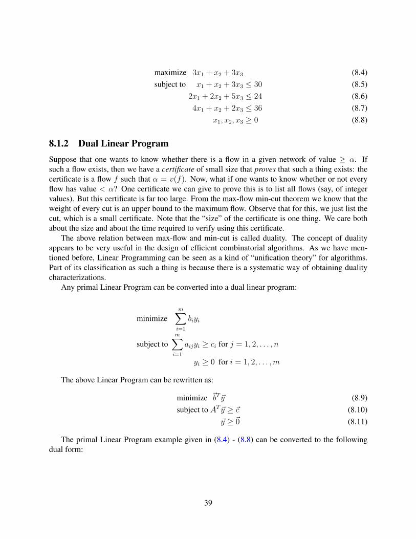
maximize 3x1 + x2 + 3x3 (8.4)subject to x1 + x2 + 3x3 ≤ 30 (8.5)
2x1 + 2x2 + 5x3 ≤ 24 (8.6)4x1 + x2 + 2x3 ≤ 36 (8.7)
x1, x2, x3 ≥ 0 (8.8)
8.1.2 Dual Linear ProgramSuppose that one wants to know whether there is a flow in a given network of value ≥ α. Ifsuch a flow exists, then we have a certificate of small size that proves that such a thing exists: thecertificate is a flow f such that α = v(f). Now, what if one wants to know whether or not everyflow has value < α? One certificate we can give to prove this is to list all flows (say, of integervalues). But this certificate is far too large. From the max-flow min-cut theorem we know that theweight of every cut is an upper bound to the maximum flow. Observe that for this, we just list thecut, which is a small certificate. Note that the “size” of the certificate is one thing. We care bothabout the size and about the time required to verify using this certificate.
The above relation between max-flow and min-cut is called duality. The concept of dualityappears to be very useful in the design of efficient combinatorial algorithms. As we have men-tioned before, Linear Programming can be seen as a kind of “unification theory” for algorithms.Part of its classification as such a thing is because there is a systematic way of obtaining dualitycharacterizations.
Any primal Linear Program can be converted into a dual linear program:
minimizem∑i=1
biyi
subject tom∑i=1
aijyi ≥ ci for j = 1, 2, . . . , n
yi ≥ 0 for i = 1, 2, . . . ,m
The above Linear Program can be rewritten as:
minimize ~bT~y (8.9)subject to AT~y ≥ ~c (8.10)
~y ≥ ~0 (8.11)
The primal Linear Program example given in (8.4) - (8.8) can be converted to the followingdual form:
39
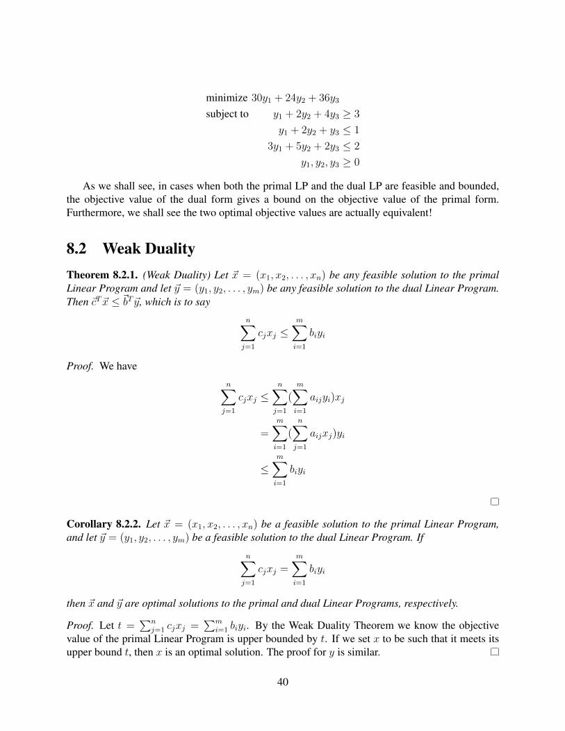
minimize 30y1 + 24y2 + 36y3
subject to y1 + 2y2 + 4y3 ≥ 3
y1 + 2y2 + y3 ≤ 1
3y1 + 5y2 + 2y3 ≤ 2
y1, y2, y3 ≥ 0
As we shall see, in cases when both the primal LP and the dual LP are feasible and bounded,the objective value of the dual form gives a bound on the objective value of the primal form.Furthermore, we shall see the two optimal objective values are actually equivalent!
8.2 Weak DualityTheorem 8.2.1. (Weak Duality) Let ~x = (x1, x2, . . . , xn) be any feasible solution to the primalLinear Program and let ~y = (y1, y2, . . . , ym) be any feasible solution to the dual Linear Program.Then ~cT~x ≤ ~bT~y, which is to say
n∑j=1
cjxj ≤m∑i=1
biyi
Proof. We have
n∑j=1
cjxj ≤n∑j=1
(m∑i=1
aijyi)xj
=m∑i=1
(n∑j=1
aijxj)yi
≤m∑i=1
biyi
Corollary 8.2.2. Let ~x = (x1, x2, . . . , xn) be a feasible solution to the primal Linear Program,and let ~y = (y1, y2, . . . , ym) be a feasible solution to the dual Linear Program. If
n∑j=1
cjxj =m∑i=1
biyi
then ~x and ~y are optimal solutions to the primal and dual Linear Programs, respectively.
Proof. Let t =∑n
j=1 cjxj =∑m
i=1 biyi. By the Weak Duality Theorem we know the objectivevalue of the primal Linear Program is upper bounded by t. If we set x to be such that it meets itsupper bound t, then x is an optimal solution. The proof for y is similar.
40
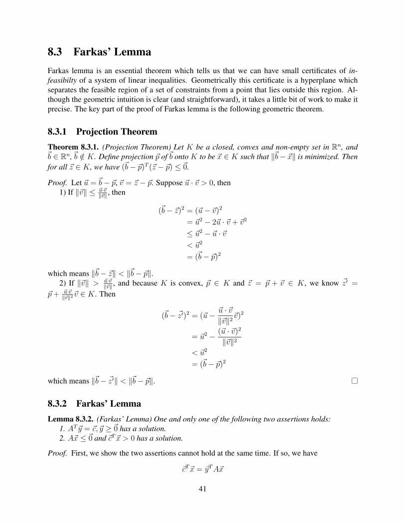
8.3 Farkas’ LemmaFarkas lemma is an essential theorem which tells us that we can have small certificates of in-feasibilty of a system of linear inequalities. Geometrically this certificate is a hyperplane whichseparates the feasible region of a set of constraints from a point that lies outside this region. Al-though the geometric intuition is clear (and straightforward), it takes a little bit of work to make itprecise. The key part of the proof of Farkas lemma is the following geometric theorem.
8.3.1 Projection TheoremTheorem 8.3.1. (Projection Theorem) Let K be a closed, convex and non-empty set in Rn, and~b ∈ Rn,~b /∈ K. Define projection ~p of~b onto K to be ~x ∈ K such that ‖~b− ~x‖ is minimized. Thenfor all ~z ∈ K, we have (~b− ~p)T (~z − ~p) ≤ ~0.
Proof. Let ~u = ~b− ~p, ~v = ~z − ~p. Suppose ~u · ~v > 0, then1) If ‖~v‖ ≤ ~u·~v
‖~v‖ , then
(~b− ~z)2 = (~u− ~v)2
= ~u2 − 2~u · ~v + ~v2
≤ ~u2 − ~u · ~v< ~u2
= (~b− ~p)2
which means ‖~b− ~z‖ < ‖~b− ~p‖.2) If ‖~v‖ > ~u·~v
‖~v‖ , and because K is convex, ~p ∈ K and ~z = ~p + ~v ∈ K, we know ~z′ =
~p+ ~u·~v‖~v‖2~v ∈ K. Then
(~b− ~z′)2 = (~u− ~u · ~v‖~v‖2
~v)2
= ~u2 − (~u · ~v)2
‖~v‖2< ~u2
= (~b− ~p)2
which means ‖~b− ~z′‖ < ‖~b− ~p‖.
8.3.2 Farkas’ LemmaLemma 8.3.2. (Farkas’ Lemma) One and only one of the following two assertions holds:
1. AT~y = ~c, ~y ≥ ~0 has a solution.2. A~x ≤ ~0 and ~cT~x > 0 has a solution.
Proof. First, we show the two assertions cannot hold at the same time. If so, we have
~cT~x = ~yTA~x
41

We know ~yT ≥ ~0 and A~x ≤ ~0. So ~cT~x = ~yTA~x ≤ 0. But this contradicts ~cT~x > 0.Next, we show at least one of the two assertions holds. Specifically, we show if Assertion 1
doesn’t hold, then Assertion 2 must hold.Assume AT~y = ~c, ~y ≥ ~0 is not feasible. Let K = AT~y : ~y ≥ ~0 (which is obviously convex).
Then ~c /∈ K. Let ~p = AT ~w(~w ≥ ~0) be the projection of ~c onto K. Then from the ProjectionTheorem we know that
(~c− AT ~w)T (AT~y − AT ~w) ≤ 0 for all ~y ≥ ~0 (8.12)
Define ~x = ~c− ~p = ~c− AT ~w. Then
~xTAT (~y − ~w) ≤ 0 for all ~y ≥ ~0(~y − ~w)TA~x ≤ 0 for all ~y ≥ ~0
Let ~ei be the n dimensional vector that has 1 in its i-th component and 0 everywhere else. Take~y = ~w + ~ei. Then
(A~x)i = ~eiTA~x ≤ 0 for i = 1, 2, . . . ,m (8.13)
Thus, each element of A~x is non-positive, which means A~x ≤ ~0.Now, ~cT~x = (~p+ ~x)T~x = ~pT~x+ ~xT~x. Setting ~y = ~0 in (8.13), we have −~wTA~x = −~pT~x ≤ ~0,
so ~pT~x ≥ 0. Since ~c 6= ~p, ~x 6= ~0, so ~xT~x > 0. Therefore, ~cT~x > 0.
8.3.3 Geometric InterpretationIf ~c lies in the cone formed by the column vectors of AT , then Assertion 1 is satisfied. Other-wise, we can find a hyperplane which contains the origin and separates ~c from the cone, and thusAssertion 2 is satisfied. These two cases are depicted below.
The ~ai’s correspond to the column vectors of AT . ~b1 and ~b2 correspond to ~c in Assertion 1 andAssertion 2, respectively.
42
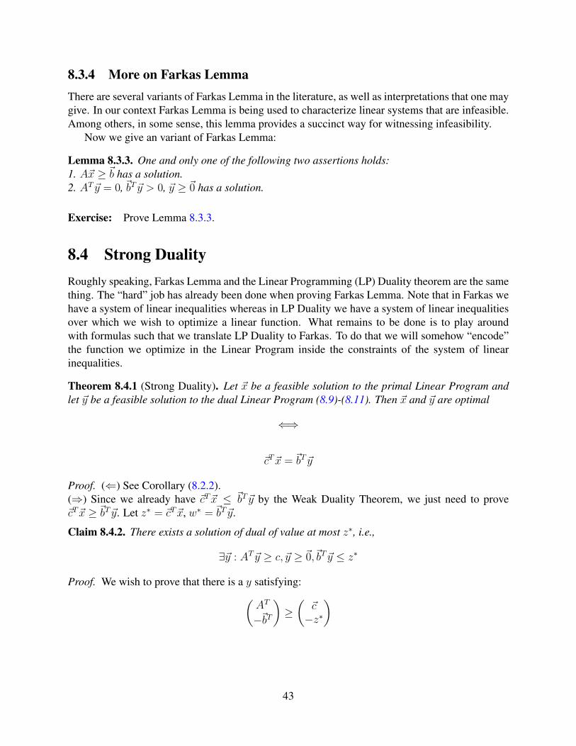
8.3.4 More on Farkas LemmaThere are several variants of Farkas Lemma in the literature, as well as interpretations that one maygive. In our context Farkas Lemma is being used to characterize linear systems that are infeasible.Among others, in some sense, this lemma provides a succinct way for witnessing infeasibility.
Now we give an variant of Farkas Lemma:
Lemma 8.3.3. One and only one of the following two assertions holds:1. A~x ≥ ~b has a solution.2. AT~y = 0,~bT~y > 0, ~y ≥ ~0 has a solution.
Exercise: Prove Lemma 8.3.3.
8.4 Strong DualityRoughly speaking, Farkas Lemma and the Linear Programming (LP) Duality theorem are the samething. The “hard” job has already been done when proving Farkas Lemma. Note that in Farkas wehave a system of linear inequalities whereas in LP Duality we have a system of linear inequalitiesover which we wish to optimize a linear function. What remains to be done is to play aroundwith formulas such that we translate LP Duality to Farkas. To do that we will somehow “encode”the function we optimize in the Linear Program inside the constraints of the system of linearinequalities.
Theorem 8.4.1 (Strong Duality). Let ~x be a feasible solution to the primal Linear Program andlet ~y be a feasible solution to the dual Linear Program (8.9)-(8.11). Then ~x and ~y are optimal
⇐⇒
~cT~x = ~bT~y
Proof. (⇐) See Corollary (8.2.2).(⇒) Since we already have ~cT~x ≤ ~bT~y by the Weak Duality Theorem, we just need to prove~cT~x ≥ ~bT~y. Let z∗ = ~cT~x, w∗ = ~bT~y.
Claim 8.4.2. There exists a solution of dual of value at most z∗, i.e.,
∃~y : AT~y ≥ c, ~y ≥ ~0,~bT~y ≤ z∗
Proof. We wish to prove that there is a y satisfying:(AT
−~bT
)≥(
~c−z∗
)
43
Assume the claim is wrong. Then the variant of Farkas’ Lemma implies that(A,−~b
)(~xλ
)= ~0(
~cT ,−z∗)(~x
λ
)> 0
~x ≥ ~0λ ≥ 0
has a solution. That is, there exist nonnegative ~x, λ such that
A~x− λ~b = ~0
~cT~x− λz∗ > 0
Case I: λ > 0. Then there exists nonnegative ~x such that A(~xλ) = ~b, ~cT (~x
λ) > z∗. This contradicts
the minimality of z∗ for the primal.
Case II: λ = 0. Then there exists nonnegative ~x such that A~x = 0, ~cT~x > 0. Take any feasiblesolution ~x′ for primal LP. Then for every µ ≥ 0, ~x′ + µ~x is feasible for primal LP, since
1. ~x′ + µ~x ≥ ~0 because ~x′ ≥ ~0, ~x ≥ ~0, µ ≥ 0.
2. A(~x′ + µ~x) = A~x′ + µA~x = ~b+ µ~0 = ~b.But ~cT (~x′+µ~x) = ~cT ~x′+~cTµ~x→∞ as µ→∞, This contradicts the assumption thatthe primal has finite solution.
The above claim shows that z∗ ≥ w∗. And we already have z∗ ≤ w∗ by Weak Duality Theorem,so z∗ = w∗
8.5 Complementary SlacknessTheorem 8.5.1. (Complementary Slackness) Let ~x be an optimal solution to the primal LinearProgram given in (8.1)-(8.3), and let ~y be an optimal solution to the dual Linear Program given in(8.9)-(8.11). Then the following conditions are necessary and sufficient for ~x and ~y to be optimal:
m∑i=1
aijyi = cj or xj = 0 for j = 1, 2, . . . , n (8.14)
n∑j=1
aijxj = bi or yi = 0 for i = 1, 2, . . . ,m (8.15)
44
Proof. (Sufficient) Define Sj = j : xj > 0 and Si = i : yj > 0. Then we have
~cT~x =n∑j=1
cjxj
=n∑
j∈Sj
cjxj
=n∑
j∈Sj
(m∑i=1
aijyi
)xj
=n∑
j∈Sj
(m∑i∈Si
aijyi
)xj
~bT~y =m∑i=1
biyi
=m∑i∈Si
biyi
=m∑i∈Si
(n∑j=1
aijxj
)yi
=m∑i∈Si
n∑j∈Sj
aijxj
yi
Therefore ~cT~x = ~bT~y. By the Strong Duality Theorem, we know ~x and ~y must be optimalsolutions.(Necessary) Suppose ~x and ~y are optimal solutions, we have
~cT~x ≤ (AT~y)T~x
=n∑j=1
(m∑i=1
aijyi
)xj
~bT~y ≥ (A~x)T~y
=m∑i=1
(n∑j=1
aijxj
)yi
~cT~x = ~bT~y
so
~cT~x = ~bT~y =n∑j=1
(m∑i=1
aijyi
)xj (8.16)
45

Suppose there exists j′ such that∑m
i=1 aij′yi > c′j and x′j > 0. Then
~cT~x =n∑j=1
cjxj
=∑j 6=j′
cjxj + cj′x′j
<∑j 6=j′
(m∑i=1
aijyi
)xj +
(m∑i=1
aij′yi
)x′j
=n∑j=1
(m∑i=1
aijyi
)xj
which contradicts optimality. Therefore equation (8.14) must be satisfied. Equation (8.15) can beproved in a similar fashion.
46
Chapter 9
Simplex Algorithm and Ellipsoid Algorithm
In this chapter, we will introduce two methods for solving Linear Programs: the simplex algorithmand the ellipsoid algorithm. To better illustrate these two algorithms, some mathematical back-ground is also introduced. The simplex algorithm doesn’t run in polynomial time, but works wellin practice. The ellipsoid runs in polynomial time, but usually performs poorly in practice.
9.1 More on Basic Feasible Solutions
9.1.1 Assumptions and conventionsSince any LP instance could be converted to maximized standard form, we’ll use the standard formof an LP to show some useful properties in the following lectures. We can write the maximizedstandard form of LP compactly as
maximize ~cT~x (9.1)subject to A~x = ~b (9.2)
~x ≥ ~0 (9.3)
We only consider the case when the LP (9.1) - (9.3) is feasible and bounded. In such cases, thefeasible region is a polytope.
Since we have seen how to convert a Linear Program from normal forms to standard form inthe previous lectures, we can simplify our notation by setting A to be an m× n matrix, ~c and ~x asn-dimensional vectors, and~b as an m-dimensional vector in (9.1) - (9.3).
It’s easy to see thatm < n. WLOG we suppose rank(A) = m so that all constraints are useful.
9.1.2 DefinitionsSuppose the Linear Program (9.1) - (9.3) is feasible and bounded. Denote the feasible region byS. It’s easy to see that S is non-empty and convex. Then we have the following definitions:
Definition 9.1.1 (Corner). A point ~x in S is said to be a corner if there is an n-dimensional vector~w and a scalar t such that
47
1. ~wT~x = t,
2. ~wT~x′ > t for all ~x′ ∈ S − ~x.
Intuitively, this definition says that all points in S are on the same side of the hyperplane Hdefined by ~w and H ∩ S = ~x. Also note that ~wT~y ≥ t for all ~y ∈ S.
Definition 9.1.2 (Extreme point). A point ~x in S is said to be an extreme point if there are no twodistinct points ~u and ~v in S such that ~x = λ~u+ (1− λ)~v for some 0 < λ < 1.
The above definition says there is no line segment in S with ~x in its interior.
Definition 9.1.3 (Basic Feasible Solution). Let B be any non-singular m×m sub-matrix made upof columns of A. If ~x ∈ S and all n −m components of ~x not associated with columns of B areequal to zero, we say ~x is a Basic Feasible Solution to A~x = ~b with respect to basis B.
Intuitively, this says that the columns ofB span the wholem-dimensional vector space. Since~bis also m-dimensional,~b is a linear composition of the columns of B. Therefore, there is a solution~x with all n−m components not associated with columns of B set to zero.
9.1.3 Equivalence of the definitionsLemma 9.1.4. If ~x is a corner, then ~x is an extreme point.
Proof. Suppose ~x is a corner, but not an extreme point. Then there exists ~y 6= ~0 such that ~x+~y ∈ Sand ~x − ~y ∈ S. So ~wT (~x + ~y) ≥ t and ~wT (~x − ~y) ≥ t. Since ~wT~x = t, we have ~wT~y ≥ 0 and~wT~y ≤ 0 which implies that ~wT~y = 0. So ~wT (~x+ ~y) = ~wT~x = t. Since ~x+ ~y ∈ S, ~x+ ~y = ~x bythe definition of corners. This means ~y = ~0, which is a contradiction.
Lemma 9.1.5. If ~x is an extreme point, then the columns ~aj : xj > 0 of A are linearly indepen-dent.
Proof. WLOG suppose the columns are ~a1, ~a2, . . . , ~ak. If they are not independent, then there arescalars d1, d2, . . . , dk not all zero such that
d1 ~a1 + d2 ~a2 + · · ·+ dk ~ak = ~0 (9.4)
WLOG we suppose |dj| < |~xj| for 1 ≤ j ≤ k. Let ~d be an n-dimensional vector such that~d = (d1, . . . , dk, 0, . . . , 0)T . Then we know
A~d = d1 ~a1 + d2 ~a2 + · · ·+ dk ~ak + 0 ~ak+1 + · · ·+ 0 ~an = ~0 (9.5)
SoA(~x+ ~d) = A~x = ~b. Since ~x+ ~d = (x1+d1, . . . , xk+dk, 0, . . . , 0) ≥ ~0, we have ~x+ ~d ∈ S.Similarly, we have ~x − ~d ∈ S. Since ~x = 1
2(~x + ~d) + 1
2(~x − ~d) and ~d 6= ~0, we see ~x is not an
extreme point, which is a contradiction.
Lemma 9.1.6. If ~x ∈ S and the columns ~aj : xj > 0 of A are linearly independent, then ~x is aBasic Feasible Solution.
48
Proof. WLOG suppose ~x = (x1, . . . , xk, 0, . . . , 0) where xj > 0 for 1 ≤ j ≤ k, which is to say,B = ~a1, . . . , ~ak are independent. Since rank(A) = m, we have k ≤ m.
1) If k = m, we are done. This is because B = [~a1 · · · ~ak] is an m×m invertible sub-matrixof A.
2) If k < m, we can widen B by incorporating more columns of A while maintaining theirindependence. Finally, B has m columns. Now the components of ~x not corresponding to thecolumns in B are still zero, so ~x is a Basic Feasible Solution.
Lemma 9.1.7. If ~x is a Basic Feasible Solution, then ~x is a corner.
Proof. WLOG suppose ~x = (x1, . . . , xm, 0, . . . , 0)T is a Basic Feasible Solution, which is to sayB = [~a1 · · · ~am] is an m ×m non-singular sub-matrix of A. Set ~w = (0, . . . , 0, 1, . . . , 1)T (withm 0’s and n−m 1’s) and t = 0. Then ~wT~x = 0. And ~wT~y ≥ 0 for any ~y ∈ S since ~y ≥ ~0.
If there exists ~z ∈ S such that ~wT~z = 0, then ~z = (z1, . . . , zm, 0, . . . , 0)T and ~b = A~z =
B[z1 · · · zm]T . Since~b = A~x = B[x1 · · · xm]T , we have [z1 · · · zm]T = [x1 · · · xm]T = B−1~b.So ~z = ~x.
Thus ~wT~x = t and ~wT~x′ > t for all ~x′ ∈ S − ~x, which proves ~x is a corner.
Now we have the following theorem stating the equivalence of the various definitions:
Theorem 9.1.8. Suppose the LP (9.1) - (9.3) is feasible with feasible region S. Then the followingstatements are equivalent:
1. ~x is a corner;
2. ~x is an extreme point;
3. ~x is a Basic Feasible Solution.
Proof. From Lemma (9.1.4) - (9.1.7).
9.1.4 Existence of Basic Feasible SolutionSo far we have seen equivalent definitions for Basic Feasible Solutions. But when do we knowwhen a BFS exists? The following theorem shows that a BFS exists if a feasible solution does.
Theorem 9.1.9. If the Linear Program (9.1) - (9.3) is feasible then there is a BFS.
Proof. Since the LP is feasible, the feasible region S 6= ∅. Let ~x be a feasible solution with aminimal number of non-zero components. If ~x = ~0, we are done since ~0 is a BFS. Otherwise, setI = i : xi > 0 then it’s clear I 6= ∅. Suppose ~x is not basic, which is to say, ai : i ∈ I are notlinearly independent. Then there exists ~u 6= ~0 with ui = 0 for i /∈ I satisfying A~u = ~0.
Consider ~x′ = ~x+ ε~u. It’s clear A~x′ = ~b for every ε. In addition, ~x′ ≥ ~0 for sufficiently small ε.So ~x′ is feasible. Increase or decrease ε until the first time one more components of ~x′ hits 0. At thatpoint, we have a feasible solution with fewer non-zero components, which is a contradiction.
49
9.1.5 Existence of optimal Basic Feasible SolutionSuppose a Linear Program is feasible and finite, i.e. has a finite optimal value. Then we can showthe LP has an optimal Basic Feasible Solution.
Theorem 9.1.10. If the Linear Program (9.1) - (9.3) is feasible and finite, there is an optimalsolution at an extreme point of the feasible region S.
Proof. Since there exists an optimal solution, there exists an optimal solution ~x with a minimalnumber of non-zero components. Suppose ~x is not an extreme point, then ~x = λ~u + (1− λ)~v forsome ~u,~v ∈ S and 0 < λ < 1. Since ~x is optimal, we must have ~cT~u ≤ ~cT~x and ~cT~v ≤ ~cT~x. Since~cT~x = λ~cT~u+ (1− λ)~cT~v, this implies ~cT~u = ~cT~v = ~cT~x. Thus ~u and ~v are also optimal.
Consider ~x′ = ~x+ ε(~u− ~v). The following statements are easy to check:
1. ~cT~x′ = ~cT~x for all ε;
2. xi = 0⇒ ui = vi = 0⇒ x′i = 0;
3. xi > 0⇒ x′i > 0 for sufficiently small ε.
Increase or decrease ε until the first time one more components of ~x′ is zero. At that point, we havean optimal solution with fewer non-zero components, which is a contradiction.
Corollary 9.1.11. If the Linear Program (9.1) - (9.3) is feasible and finite, then there is an optimalBasic Feasible Solution.
Proof. From Theorem (9.1.8) and Theorem (9.1.10).
9.2 Simplex algorithm
9.2.1 The algorithmThe simplex algorithm is based on the existence of an optimal Basic Feasible Solution(BFS). Thealgorithm first chooses a BFS (or reports the LP is infeasible), then in each iteration, moves fromthe BFS to its neighbor (which differs from it in one column), and makes sure the objective valuedoesn’t decrease when all non-basic variables are set to zero. This is called pivoting.
Consider the following example:
z = 27 +x24
+x32− 3x6
4
x1 = 9 − x24− x3
2− x6
4
x4 = 21− 3x24− 5x3
2+
x64
x5 = 6 − 3x22− 4x3 +
x62
50

In this LP, x1, x4, x5 is a BFS. If we set non-basic variables to zero, the objective value is 27.After a pivoting with x3 joining the BFS and x5 leaving the BFS, it becomes:
z =111
4+
x216− x5
8− 11x6
16
x1 =33
4− x2
16+
x58− 5x6
16
x3 =3
2− 3x2
8− x5
4+
x68
x4 =69
4+
3x216
+5x58− x6
16
In this LP, x1, x3, x4 is a BFS. If we set non-basic variables to zero, the objective value is1114> 27. If we continue pivoting, either we reach the optimal BFS, or we conclude the LP is
unbounded.To prevent cycling, we can use Bland’s rule, which says we should choose the variable with
the smallest index for tie-breaking.Interested readers should refer to Introduction to Algorithms, Chapter 29 for more details of
the simplex algorithm. In particular, this will illustrate:
1. How to choose the initial BFS.
2. How to choose the pivoting element.
3. When to assert the LP is infeasible, unbounded or whether an optimal solution can found.
9.2.2 EfficiencyThe simplex algorithm is not a polynomial time algorithm. Klee and Minty gave an exampleshowing that the worst-case time complexity of simplex algorithm is exponential in 1972. But it isgenerally fast in real world applications.
9.3 Ellipsoid algorithmIn this section, we only consider when a finite feasible region exists.
9.3.1 HistoryIf we formulate an LP in its decision version, then it’s obvious LP ∈ NP since a NTM can nonde-terministically guess the solution. In addition, LP ∈ co-NP since an NTM can guess the solutionto the LP’s dual. So LP ∈ NP ∩ co-NP. However, it was not until Khachiyan posted his ellipsoidalgorithm, a polynomial time algorithm, that people knew LP ∈ P.
51
9.3.2 Mathematical backgroundCaratheodory’s theorem
Theorem 9.3.1 (Caratheodory’s theorem). If a point ~x of Rd lies in the convex hull of a set P , thereis a subset P ′ of P consisting of d + 1 or fewer points which are affinely independent such that ~xlies in the convex hull of P . Equivalently, ~x lies in an r-simplex with vertices in P , where r ≤ d.
Proof. Let ~x be a point in the convex hull of P . Then, ~x is a convex combination of a finite numberof points in P :
~x =k∑j=1
λjxj
where every xj is in P , every λj is positive, and∑k
j=1 λj = 1.If x2 − x1, . . . , xk − x1 are linearly independent, there are scalars µ2, . . . , µk not all zero such
thatk∑j=2
µj(xj − x1) = 0
If µ1 is defined as µ1 = −∑k
j=2 µj , then∑k
j=1 µjxj = 0 and∑k
j=1 µj = 0 and not all of theµj’s are equal to zero. Therefore, at least one µj > 0. Then,
~x =k∑j=1
λjxj − αk∑j=1
µjxj =k∑j=1
(λj − αµj)xj
for any real α. In particular, the equality will hold if α is defined as
α = min1≤j≤k
λjµj
: µj > 0
= λiµi.
Note that α > 0, and for every j between 1 and k, λj − αµj ≥ 0. In particular, λi − αµi = 0by definition of α. Therefore,
~x =k∑j=1
(λj − αµj)xj
where every λjαµj is non-negative, their sum is one, and furthermore, λiαµi = 0. In otherwords, ~x is represented as a convex combination of one less point of P .
Note that if k > d + 1, x2 − x1, . . . , xk − x1 are always linearly dependent. Therefore, thisprocess can be repeated until ~x is represented as a convex combination of r ≤ d + 1 pointsxi1 , . . . , xir in P . Since xi2 − xi1 , . . . , xir − xi1 are linearly independent, when this process termi-nates, xi1 , . . . , xir are affinely independent.
Quadratic form
~xTA~x is called a quadratic form, where ~x is an n-dimensional vector and A is a symmetric n× nmatrix. If A is positive definite, then ~xTA~x = 1 is an ellipsoid.
52

Volume of n-simplices
A set of n + 1 affinely independent points S ∈ Rn make up an n-simplex. The volume of thisn-simplex is
1
n!|det
(1 1 · · · 1p0 p1 · · · pn
)|
9.3.3 LP,LI and LSIThere are three kinds of problems that are related to each other.
Question: [Linear Programming/IP] Given an integerm×nmatrixA,m-vector~b and n-vector~c, either
(a) Find a rational n-vector ~x such that ~x ≥ ~0, A~x = ~b and ~cT~x is minimized subject to theseconditions, or
(b) Report that there is no n-vector ~x such that ~x ≥ ~0 and A~x = ~b, or(c) Report that the set ~cT~x : A~x = ~b, ~x ≥ ~0 has no lower bound.Question: (Linear Inequalities) Given an integer m × n matrix A and m-vector ~b, is there an
n-vector ~x such that A~x ≤ ~b?Question: (Linear Strict Inequalities/LSI) Given an integer m×n matrix A and m-vector~b, is
there an n-vector ~x such that A~x <~b?
Polynomial reductions
Theorem 9.3.2. There is a polynomial-time algorithm for an LP if and only if there is a polynomial-time algorithm for LI.
Theorem 9.3.3. If there is a polynomial-time algorithm for LSI then there is a polynomial-timealgorithm for LI.
Therefore, we just need to provide an polynomial-time algorithm for LSI to ensure there is apolynomial-time algorithm for LP, via the reduction LP ≤ LI ≤ LSI.
9.3.4 Ellipsoid algorithmThe main idea of the ellipsoid algorithm is to do a binary search. Initially the algorithm findsan ellipsoid large enough so that a part of the feasible region with lower-bounded volume v0 iscontained within it. In each iteration, the algorithm tests whether the center of the ellipsoid is afeasible solution. If so, it reports success. Otherwise, it finds a constraint that is violated, whichdefines a hyperplane. Since the center is on the wrong side of this hyperplane, at least half of theellipsoid can be discarded. The algorithm proceeds by finding a smaller ellipsoid which containsthe half of the original ellipsoid which is on the correct side. The ratio between the volume of thenew ellipsoid and that of the old one is upper bounded by r(n) < 1. Therefore, after (polynomially)many iterations, either a solution is found, or the ellipsoid becomes small enough (the volume ofit is less than v0) such that no feasible region can be contained in it. In the latter case, the feasibleregion is can be declared empty.
53

The whole algorithm is given below:Algorithm 8: Ellipsoid algorithm
input : An m× n system of linear strict inequalities A~x <~b, of size Loutput: an n-vector such that A~x <~b, if such a vector exists; ‘no’ otherwise1. InitializeSet j = 0, ~t0 = ~0, B0 = n222L · I ./* j counts the number of iterations so far. */
/* The current ellipsoid is Ej = ~x : (~x− ~tj)TB−1j (~x− ~tj) ≤ 1 */2. Testif ~tj is a solution to A~x <~b then
return ~tjendif j > K = 16n(n+ 1)L then
return’no’end3. Iterate:Choose any inequality in A~x <~b that is violated by ~tj; say ~aT ~tj ≥ ~b.Set
~tj+1 = ~tj −1
n+ 1
Bja√atBja
Bj+1 =n2
n2 − 1(Bj −
2
n+ 1
(Bja)(Bja)T
aTBja)
j = j + 1
Goto 2.
Theorem 9.3.4. Ellipsoid algorithm runs in polynomial time.
Proof. The algorithm runs for at most 16n(n+1)L rounds, and each round takes polynomial time.So the algorithm runs in polynomial time.
54

Chapter 10
Max-Flow Min-Cut Through LinearProgramming
In this chapter, we give a proof of the Max-Flow Min-Cut Theorem using Linear Programming.
10.1 Flow and CutFirst, we review the definition of Max-Flow and Min-Cut and introduce another definition of Max-Flow.
10.1.1 FlowLet N = (G, s, t, c) be a network (directed graph) with s and t the source and the sink of N ,respectively. The capacity of an edge is a mapping c: E → R+, denoted by cuv or c(u, v); thisrepresents the maximum amount of “flow” that can pass through an edge.
Definition 10.1.1 (Flow). A flow is a mapping f: E → R+, denoted by fuv or f(u, v), subject tothe following two constraints:
1. fuv ≤ cuv for each (u, v) ∈ E (capacity constraint)
2.∑
u: (u,v)∈E fuv =∑
u: (v,u)∈E fvu for each v ∈ V \ s, t (conservation constraint).
The value of flow represents the amount of flow passing from the source to the sink and isdefined by val(f) =
∑v∈V fsv, where s is the source of N . The maximum flow problem is to
maximize val(f), i.e. to route as much flow as possible from s to the t.
Definition 10.1.2 (Path). A path is a sequence of vertices such that there is a directed path fromone vertex to next vertex in the sequence. An s− t path is a path that with s at the beginning of thesequence and vertex t the last.
55

10.1.2 An alternative Definition of FlowWe currently give another definition of flow, and later prove that it is equivalent to Definition 10.1.1.
Definition 10.1.3 (Flow (alternate)). In N = (G, s, t, c), let P be the set of vertices that constitutethe s− t path. A flow is a mapping f’: P → R+ , denoted by f ′p or f ′(p), subject to the followingconstraint:
1.∑
p: (u,v)∈p f′p ≤ cuv for each (u, v) ∈ E
The value of flow is defined by val(f ′) =∑
p∈P f′p.
10.1.3 CutDefinition 10.1.4 (Cut). An s-t cut C = (S, T ) is a partition of V such that s ∈ S and t ∈ T .
Definition 10.1.5 (Cut Set). The cut-set of C is the set (u, v) ∈ E|u ∈ S, v ∈ T.Note that if the edges in the cut-set of C are removed, val(f) = 0.
Definition 10.1.6 (Capacity). The capacity of an s− t cut is defined by c(S, T ) =∑
(u,v)∈S×T cuv.
The minimum cut problem is to minimize c(S, T ), i.e. to determine an S and T such that thecapacity of the S-T cut is minimal.
10.2 Max-flow Min-Cut TheoremIn this section, we prove the Max-Flow and Min-Cut Theorem by using Linear Programming.Before we go into the proof, we need the following two lemmas.
Lemma 10.2.1. Given N = (G, s, t, c), for every flow val(f) > 0, there exist an s− t path p suchthat ∀(u, v) ∈ p, fuv > 0
Proof. We prove the lemma by contradiction.If such an s − t path does not exist, let A = v ∈ V |∃ s-v path p, ∀(u,w) ∈ p, fuw > 0. Thens ∈ A, t 6∈ A and ∀u ∈ A, v 6∈ A, fuv = 0.∑
v∈A
(∑
w: (v,w)∈E
fvw −∑
u: (u,v)∈E
fuv) =∑
w: (s,w)∈E
fsw
= val(f)
> 0
But ∑v∈A
(∑
w: (v,w)∈E
fvw −∑
u: (u,v)∈E
fuv) =∑
v∈A,w 6∈A,(v,w)∈E
fvw −∑
u6∈A,v∈A,(u,v)∈E
fuv
= −∑
u6∈A,v∈A,(u,v)∈E
fuv
≤ 0
This is a contradiction.
56
Lemma 10.2.2 (Flow Decomposition). The two definitions of flow 10.1.1 and 10.1.3 are equiva-lent. In N = (G, s, t, c), for every α ∈ R+,
∃f : E → R+, val(f) = α⇔ ∃f ′ : P → R+, val(f ′) = α
Proof. (⇐) Let fuv =∑
p: (u,v)∈p f′p.
• First we prove that f is a flow by examining the two constraints given in Definition 10.1.1.For the capacity constraint, we know by Definition 10.1.3 of f ′, fuv ≤ cuv for each (u, v) ∈E.For the conservation constraint, by the definition of path 10.1.2, for every path p, ∀(u, v) ∈p,∃(v, w) ∈ p and ∀(v, w) ∈ p, ∃(u, v) ∈ p.Thus, for every path p and node v , |(u, v) ∈ p|u ∈ V | = |(v, w) ∈ p|w ∈ V |. So forevery v ∈ V ∑
p∈P
∑u: (u,v)∈p
f ′p =∑p∈P
∑w: (v,w)∈p
f ′p
=⇒∑
u: (u,v)∈E
fuv =∑
u: (v,u)∈E
fvu
• Second we prove that val(f) = val(f ′)
val(f) =∑v∈V
fsv =∑v∈V
∑(s,v)∈p
f ′p =∑p∈P
f ′p = val(f ′)
(⇒) We prove this direction by induction on |E|,
• The base case is obvious when |E| ≤ 2,
• For the inductive step, if val(f) = 0, let f ′p = 0.If |f | > 0, then by Lemma 10.2.1 there exists an s− t path p. Let α = minfuv ,(u,v)∈p, α > 0.
We construct a new flow f1 by reducing fuv by α for every (u, v) ∈ p and then remove alledges (u, v) such that f(u, v) = 0. In the new flow, at least one edge is removed; thus, byinduction, ∃val(f ′1) = val(f1). We can then get f ′ by adding p to f ′1.Thus we find
val(f ′) = val(f ′1) + α = val(f1) + α = val(f)
Theorem 10.2.3 (Max-flow Min-cut Theorem). Given N = (G, s, t, c), maxval(f) : E →R+ = minval(f ′) : P → R+
Proof Sketch: 1. Get the LP of the max-flow problem according to the Definition 10.1.3.
2. Find the dual of the LP. The equivalence of the two answers are guaranteed by the strongduality theorem.
57
3. Prove the solution of the dual is equal to the answer of the min-cut problem.
Proof. First, we present an LP of the max-flow problem along with its dual.
Max-flow Dualmaximize: val(f ′) =
∑p∈P f
′p
subject to:∑(u,v)∈p f
′p ≤ cuv (u, v) ∈ Ef ′p ≥ 0 p ∈ P
minimize:∑
(u,v)∈E cuvyuvsubject to:∑
(u,v)∈p yuv ≥ 1 p ∈ Pyuv ≥ 0 (u, v) ∈ E
We prove the solution of the dual LP is equivalent to that of the min-cut of N via the followingtwo observations.
Observation 10.2.4. In N , ∀ cuts C = (S, T ), there is a feasible solution to the dual LP of max-follow in N with cost equal to c(S, T ).
Proof. For C = (S, T ), set
yuv =
1 u ∈ S, v ∈ T0 otherwise
It is easy to check that this is a feasible solution of the dual LP and the cost is equal to c(S, T ).
Observation 10.2.5. In N = (V,E), given a feasible solution yuv(u,v)∈E to the dual LP, ∃C =(S, T ), where c(S, T ) is less than or equal to the cost of the solution.
Proof. First, construct a graph G = (V,E), where the distance between u and v is given bydis(u, v) = yuv, (u, v) ∈ E.Let d(u, v) be the length of shortest path from u to v according to dis.Thus the first |P | constraints of the dual LP can be written as
d(s, t) ≥ 1
Clearly, this stipulates that all paths from s to t should be greater than 1.Pick a uniform random number T ∈ [0, 1).For a given T , we construct a cut in the following way,
v ∈S d(s, v) ≤ TT d(s, v) > T
We define the following function to make things more clear.
In(u, v, S, T ) =
1 u ∈ S, v ∈ T0 otherwise
58

We prove that the expectation of c(S, T ) is equal to the cost of the solution of the dual LP.
E(c(S, T )) =∑
(u,v)∈E
E(cuvIn(u, v, S, T )) (10.1)
=∑
(u,v)∈E
cuvE(In(u, v, S, T )) (10.2)
=∑
(u,v)∈E
cuv Pr(u ∈ S, v ∈ T ) (10.3)
=∑
(u,v)∈E
cuv Pr(d(s, u) ≤ T ∧ d(s, v) > T ) (10.4)
≤∑
(u,v)∈E
cuv(d(s, v)− d(s, u)) (10.5)
≤∑
(u,v)∈E
cuv · dis(u, v) (10.6)
=∑
(u,v)∈E)
cuvyuv (10.7)
Because the expectation of c(S, T ) equals to the cost of the solution, then there must exist a cutC = (S, T ) which is less than or equal to the cost of the solution.
According to Observation 10.2.4, we know that the minimum cost of the solution of the dualLP is less or equal to that of min-cut the problem.According to Observation 10.2.5, we know that the solution to the min-cut problem is less than orequal to the minimum cost of the solution of the dual LP.Thus, we arrive at the conclusion that the solution of the dual must exactly equal to that of themin-cut problem.
The proof of Max-flow Min-cut Theorem immediately follows.
59

Chapter 11
Rounding Technique for ApproximationAlgorithms(I)
In this chapter, we give some concrete examples about using Linear Programming to solve opti-mization problems. First, we give the general method to solve problems using LPs. Then, we givethe Set Cover problem as an example to the general method. We give two approximation algo-rithms for Set Cover and apply LP-rounding on the Vertex Cover problem to get a 2-approximationalgorithm.
11.1 General Method to Use Linear ProgrammingHere, we show the general idea to solve problems using an LP.
To make things easier to understand, we will provide three examples of problems solved byLinear Programing: Set Cover, Vertex Cover and MAX-K SAT.
11.2 Set Cover Problem
11.2.1 Problem DescriptionWe are given a set U of n elements e1, e2, · · · , en, and a set S of k subsets S1, S2, · · · , Sk fromU. A set cover is a collection of subsets from S that satisfy the condition that every element in Ubelongs to one of the subsets. In addition, we are given a cost function c : S → Z+. The cost of aset cover is denoted by the sum of costs of each subset in the collection of selected subsets S. Ourobjective is to find the collection of subsets that minimizes the cost.
Example 11.2.1. U = 1, 2, · · · , 6 and S′ = S1, S2, S3 where S1 = 1, 2, S2 = 2, 3, 4 andS3 = 5, 6. In addition, we have the cost of the three sets are 1, 2 and 3 respectively. The exampleis illustrated below:
60
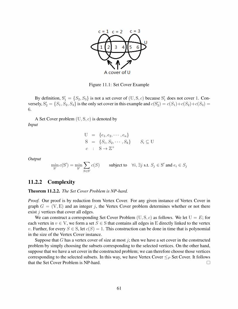
Figure 11.1: Set Cover Example
By definition, S′1 = S2, S3 is not a set cover of (U, S, c) because S′1 does not cover 1. Con-versely, S′2 = S1, S2, S3 is the only set cover in this example and c(S′2) = c(S1)+c(S2)+c(S3) =6.
A Set Cover problem (U, S, c) is denoted byInput
U = e1, e2, · · · , enS = S1, S2, · · · , Sk Si ⊆ U
c : S→ Z+
OutputminS′
c(S′) = minS′
∑S∈S′
c(S) subject to ∀i, ∃j s.t. Sj ∈ S′ and ei ∈ Sj
11.2.2 ComplexityTheorem 11.2.2. The Set Cover Problem is NP-hard.
Proof. Our proof is by reduction from Vertex Cover. For any given instance of Vertex Cover ingraph G = (V,E) and an integer j, the Vertex Cover problem determines whether or not thereexist j vertices that cover all edges.
We can construct a corresponding Set Cover Problem (U, S, c) as follows. We let U = E; foreach vertex in v ∈ V, we form a set S ∈ S that contains all edges in E directly linked to the vertexv. Further, for every S ∈ S, let c(S) = 1. This construction can be done in time that is polynomialin the size of the Vertex Cover instance.
Suppose that G has a vertex cover of size at most j; then we have a set cover in the constructedproblem by simply choosing the subsets corresponding to the selected vertices. On the other hand,suppose that we have a set cover in the constructed problem; we can therefore choose those verticescorresponding to the selected subsets. In this way, we have Vertex Cover ≤P Set Cover. It followsthat the Set Cover Problem is NP-hard.
61
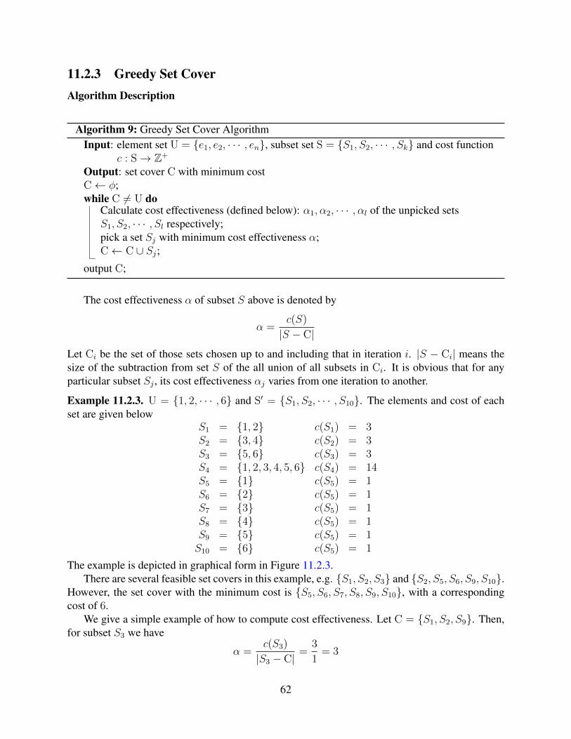
11.2.3 Greedy Set CoverAlgorithm Description
Algorithm 9: Greedy Set Cover AlgorithmInput: element set U = e1, e2, · · · , en, subset set S = S1, S2, · · · , Sk and cost function
c : S→ Z+
Output: set cover C with minimum costC← φ;while C 6= U do
Calculate cost effectiveness (defined below): α1, α2, · · · , αl of the unpicked setsS1, S2, · · · , Sl respectively;pick a set Sj with minimum cost effectiveness α;C← C ∪ Sj;
output C;
The cost effectiveness α of subset S above is denoted by
α =c(S)
|S − C|
Let Ci be the set of those sets chosen up to and including that in iteration i. |S − Ci| means thesize of the subtraction from set S of the all union of all subsets in Ci. It is obvious that for anyparticular subset Sj , its cost effectiveness αj varies from one iteration to another.
Example 11.2.3. U = 1, 2, · · · , 6 and S′ = S1, S2, · · · , S10. The elements and cost of eachset are given below
S1 = 1, 2 c(S1) = 3S2 = 3, 4 c(S2) = 3S3 = 5, 6 c(S3) = 3S4 = 1, 2, 3, 4, 5, 6 c(S4) = 14S5 = 1 c(S5) = 1S6 = 2 c(S5) = 1S7 = 3 c(S5) = 1S8 = 4 c(S5) = 1S9 = 5 c(S5) = 1S10 = 6 c(S5) = 1
The example is depicted in graphical form in Figure 11.2.3.There are several feasible set covers in this example, e.g. S1, S2, S3 and S2, S5, S6, S9, S10.
However, the set cover with the minimum cost is S5, S6, S7, S8, S9, S10, with a correspondingcost of 6.
We give a simple example of how to compute cost effectiveness. Let C = S1, S2, S9. Then,for subset S3 we have
α =c(S3)
|S3 − C|=
3
1= 3
62
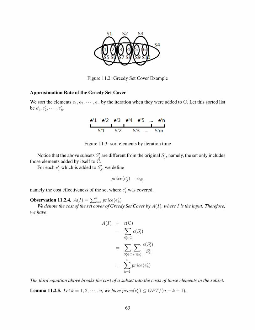
Figure 11.2: Greedy Set Cover Example
Approximation Rate of the Greedy Set Cover
We sort the elements e1, e2, · · · , en by the iteration when they were added to C. Let this sorted listbe e′1, e
′2, · · · , e′n.
Figure 11.3: sort elements by iteration time
Notice that the above subsets S ′j are different from the original S ′j , namely, the set only includesthose elements added by itself to C.
For each e′j which is added to S ′j , we define
price(e′j) = αS′j
namely the cost effectiveness of the set where e′j was covered.
Observation 11.2.4. A(I) =∑n
k=1 price(e′k)
We denote the cost of the set cover of Greedy Set Cover byA(I), where I is the input. Therefore,we have
A(I) = c(C)
=∑S′i∈C
c(S ′i)
=∑S′i∈C
∑e′∈S′i
c(S ′i)
|S ′i|
=n∑k=1
price(e′k)
The third equation above breaks the cost of a subset into the costs of those elements in the subset.
Lemma 11.2.5. Let k = 1, 2, · · · , n, we have price(e′k) ≤ OPT/(n− k + 1).
63

Proof. Note that the remaining elements e′k, e′k+1, · · · , e′n can be covered at cost at most OPT,
namely in the OPT solution of the problem. Therefore, there is a subset in OPT which has not beenselected and with a cost effectiveness at most OPT/(n−k+ 1). Further, our algorithm chooses tocover a set with minimum cost effectiveness, so that we should have price(e′k) ≤ OPT/(n−k+1)to guarantee our algorithm could pick the selected subset.
Theorem 11.2.6. Greedy Set Cover is ln(n)-approx
Proof.
A(I) =n∑k=1
price(e′k)
≤ (1
n+
1
n− 1+ · · ·+ 1
2+ 1)OPT
≤ dln(n)eOPT
The first equation is due to Observation 11.2.4, and the second is derived from the above lemma.Thus, the Greedy Set Cover is an ln(n)-approximation algorithm.
Tightness of Greedy Set Cover
U = e1, e2, · · · , en and S = S1, S2, · · · , Sn. The elements and cost of each set is given below:
S1 = 1 c(S1) = 1/nS2 = 2 c(S2) = 1/(n− 1)S3 = 3 c(S3) = 1/(n− 2)
. .
. .
. .Sn−1 = n− 1 c(Sn−1) = 1/2Sn = 1, 2, · · · , n c(Sn) = 1 + ε
The ε above is some negligible value. It is obvious that the OPT Set Cover is Sn with cost n.However, in our algorithm, in iteration i we will pick the Sj that has the minimum cost effective-ness. The ε is used here to make sure the cost effectiveness of Sj is smaller that of Sn. In this way,we will choose all n subsets and get a solution with cost
1
n+
1
n− 1+ · · ·+ 1 = dln(n)e
So we construct a worst case for any n with approximation ratio ln(n). In conclusion, the ln(n)approximation is tight for Greedy Set Cover.
64
11.2.4 LP-rounding Set CoverInteger Program
We express the Set Cover problem as an Integer Programs in the following form:Minimize
k∑i=1
c(Si)ui
Subject to ∑i:e∈Si
ui ≥ 1 , ∀e ∈ Uui ∈ 0, 1 , i = 1, 2, · · · , k
where ui is the boolean variable that shows whether or not set Si has been chosen. Si is not chosenwhen ui = 0, while Si is chosen when ui = 1.
Example 11.2.7. U = 1, 2, 3, 4 and the sets and cost of each are given below:
S1 = 1, 2 c(S1) = 5S2 = 2, 3 c(S2) = 100S3 = 2, 3, 4 c(S3) = 1
We can change the set cover problem above into the integer programs as follows:Minimize
5u1 + 100u2 + u3
Subject to1 : u1 ≥ 12 : u1 + u2 + u3 ≥ 13 : u2 + u3 ≥ 14 : u3 ≥ 1
ui ∈ 0, 1 i ∈ 1, 2, 3
Relaxing to a Linear Program
The above construction an Integer Program properly represents the original Set Cover problem;however, the Integer Program is still NP-hard.
To get an approximation algorithm, we relax the integral constraints and get a Linear Program.
Integer Program Linear ProgramMinimize :
∑ki=1 uic(Si)
Subject to:∑i:e∈Si
ui ≥ 1 , ∀e ∈ Uui ∈ 0, 1 , i = 1, 2, · · · , k
Minimize :∑k
i=1 uic(Si)Subject to:∑
i:e∈Siui ≥ 1 , ∀e ∈ U
0 ≤ ui ≤ 1 , i = 1, 2, · · · , k
We relax only the non-linear constraints for ui. In this way, we can easily solve the LinearProgram in polynomial time. However, the relaxation of constraints brings about a new problem:How can we interpret the result vector u = (u1, u2, · · · , uk) when some ui’s are fractions?
65

Algorithm 10: LP-rounding Set Cover AlgorithmInput: element set U = e1, e2, · · · , en, subset set S = S1, S2, · · · , Sk and cost function
c : S→ Z+
Output: set cover C with minimum cost
1. Write the original Set Cover problem as an Integer Program.
2. Relax the Integer Program into a Linear Program.
3. Solve the Linear Program using the Ellipsoid Algorithm and obtain~u = (u1, u2, · · · , uk) ∈ Rk.
4. Let f be the maximum frequency (the number of times that element appears in distinctsubsets).
5. Output deterministic rounding ~u′ = (u′1, u′2, · · · , u′k) ∈ 0, 1k, where u′i satisfies
u′i =
1 , ui ≥ 1/f0 , otherwise
LP-rounding Set Cover Algorithm
The algorithm first changes the original Set Cover problem into an Integer Program, then relaxesthe constraints of the IP to obtain a Linear Program. By solving this LP, we get a solution ~u ∈ Rk.Lastly, we round each element of the result vector ~u using the f below.
Effectiveness of LP-rounding
Lemma 11.2.8. LP-rounding Set Cover is an f -approximation.
Proof. First, we prove that ~u′ is a feasible solution. In order to show this, we need to examine eachconstraint and satisfy it. Suppose
u1 + u2 + · · ·+ ul ≥ 1
be one of the constraints. By definition, we have l ≤ f . Now, there must be some i such thatui ≥ 1/l ≥ 1/f . In this way, ui will be rounded to 1, and therefore satisfies the proper constraint.Thus, the resulting vector ~u′ is a feasible solution.
On the other hand, we look into the rounding process from ui to u′i:
u′i =
1 , ui ≥ 1/f0 , otherwise
66
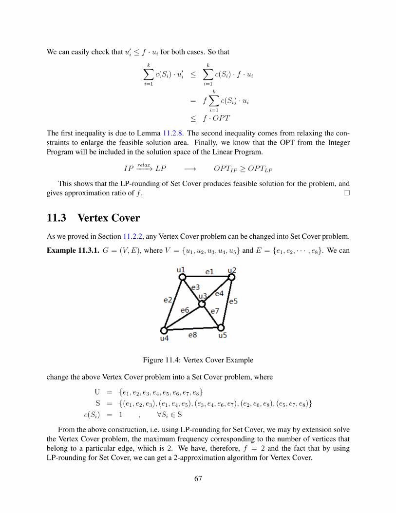
We can easily check that u′i ≤ f · ui for both cases. So that
k∑i=1
c(Si) · u′i ≤k∑i=1
c(Si) · f · ui
= f
k∑i=1
c(Si) · ui
≤ f ·OPT
The first inequality is due to Lemma 11.2.8. The second inequality comes from relaxing the con-straints to enlarge the feasible solution area. Finally, we know that the OPT from the IntegerProgram will be included in the solution space of the Linear Program.
IPrelax−−−→ LP −→ OPTIP ≥ OPTLP
This shows that the LP-rounding of Set Cover produces feasible solution for the problem, andgives approximation ratio of f .
11.3 Vertex CoverAs we proved in Section 11.2.2, any Vertex Cover problem can be changed into Set Cover problem.
Example 11.3.1. G = (V,E), where V = u1, u2, u3, u4, u5 and E = e1, e2, · · · , e8. We can
Figure 11.4: Vertex Cover Example
change the above Vertex Cover problem into a Set Cover problem, where
U = e1, e2, e3, e4, e5, e6, e7, e8S = (e1, e2, e3), (e1, e4, e5), (e3, e4, e6, e7), (e2, e6, e8), (e5, e7, e8)
c(Si) = 1 , ∀Si ∈ S
From the above construction, i.e. using LP-rounding for Set Cover, we may by extension solvethe Vertex Cover problem, the maximum frequency corresponding to the number of vertices thatbelong to a particular edge, which is 2. We have, therefore, f = 2 and the fact that by usingLP-rounding for Set Cover, we can get a 2-approximation algorithm for Vertex Cover.
67
Chapter 12
Rounding Technique for ApproximationAlgorithms(II)
In this chapter, we will give a randomized algorithm for Set Cover. The algorithm gives an approx-imation factor of log n for Set Cover, and reaches this approximation ratio with high probability.Then, we give a randomized algorithm for the MAX-K SAT problem. Furthermore, we will give adeterministic algorithm which derandomizes the aforementioned MAX-K SAT algorithm using themethod of conditional expectation.
12.1 Randomized Algorithm for Integer Program of Set Cover
12.1.1 Algorithm DescriptionWe know from the previous lecture how to express the Set Cover problem as a Linear Program.For the randomized algorithm, we do the same thing as the last lecture, perform a linear relaxation.
Minimize :k∑i=1
uic(Si)
Subject to: ∑i:e∈Si
ui ≥ 1 , ∀e ∈ Uui ∈ [0, 1] , i = 1, 2, · · · , k
Here is the algorithm:
12.1.2 The correctness of the AlgorithmFirstly, we want to know the expectation of C(G), where C(G) is the configuration of a randomcollection of sets in all iterations. Assume G is the random collection of sets in one iteration. Then
68

Algorithm 11: LP-rounding Set Cover AlgorithmInput: element set U = e1, e2, · · · , en, subset set S = S1, S2, · · · , Sk and cost function
c : S→ Z+
Output: set cover C with minimum cost
1. Solve the LP-rounding Set Cover, and let the solution be (x1, x2 . . . xn) ∈ Rn(e.g. using theEllipsoid algorithm)
2. Randomly choose u′i ∈R [0, 1]
If u′i ≤ xi, ui ← 1, otherwise ui ← 0
Then Pr(ui = 1) = xi and Pr(ui = 0) = 1− xi
3. Repeat the second step 2 lnn times. Output the collection G of sets corresponding to ui (Ifui = 1, then we picked Si into G)
the expectation of C(G) is
E[C(G)] =k∑i=1
Pr(Si is picked)C(Si)
=k∑i=1
xiC(Si)
= OPTfractional
≤ OPT
So the expectation of C(G) is
E[C(G)] ≤ 2 lnn× E[C(G)]
≤ (2 lnn)OPTfraction
≤ 2 lnnOPT
Markov’s inequality:
Pr(|X| ≥ α) ≤ E(|X|)a
Using Markov’s inequality, we have
Pr[C(G) ≥ 8 lnnOPT ] ≤ 1
4
Now, we want to know the probability that every ei has been covered. We know one element is
69

not covered during one iteration of step 2 in algorithm with probability
Pr[e is not covered in one iteration] =∏i:e∈Si
(1− xi)
≤∏i:e∈Si
e−xi
= e−∑
i:e∈Sixi
≤ 1
e
The last inequality is due to∑
i:e∈Sixi ≥ 1
Then the probability that e is not covered in any of the 2 lnn repetitions is:
P ≤ (1
e)2 lnn ≤ (
1
n)2 =
1
n2
We know that:Pr(A ∨B) ≤ Pr(A) + Pr(B)
So the probability of having an element which is not covered is:
Pr[∃eis not covered] = Pr[e1 is not covered ∨ e2 is not covered · · · ∨ en is not covered]
≤ 1
n2· n
=1
n
SoPr[all elements are covered] ≥ 1− 1
n
Let E be the event that all elements are covered and E ′ be the event that C(G) ≥ 8 lnn ·OPT .Then we have:
Pr[E ′ ∧ E ] ≥ 1− 1
n− 1
4
>2
3
Hence, we have an algorithm that succeeds with probability higher than 12. Using Chernoff
bounds we can repeat the algorithm a polynomial number of times so as to succeed with highprobability.
12.2 Method of Computation Expectations
12.2.1 MAX-K-SAT problemLet us introduce the MAX-K-SAT problem.
70
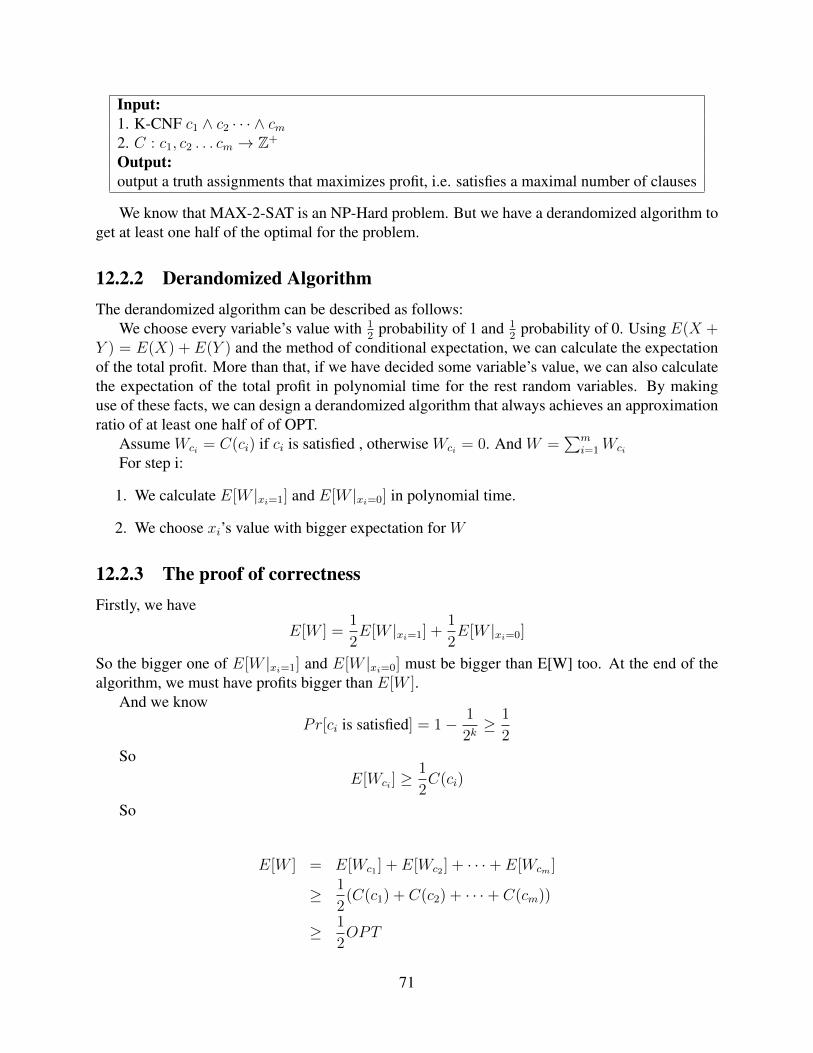
Input:1. K-CNF c1 ∧ c2 · · · ∧ cm2. C : c1, c2 . . . cm → Z+
Output:output a truth assignments that maximizes profit, i.e. satisfies a maximal number of clauses
We know that MAX-2-SAT is an NP-Hard problem. But we have a derandomized algorithm toget at least one half of the optimal for the problem.
12.2.2 Derandomized AlgorithmThe derandomized algorithm can be described as follows:
We choose every variable’s value with 12
probability of 1 and 12
probability of 0. Using E(X +Y ) = E(X) + E(Y ) and the method of conditional expectation, we can calculate the expectationof the total profit. More than that, if we have decided some variable’s value, we can also calculatethe expectation of the total profit in polynomial time for the rest random variables. By makinguse of these facts, we can design a derandomized algorithm that always achieves an approximationratio of at least one half of of OPT.
Assume Wci = C(ci) if ci is satisfied , otherwise Wci = 0. And W =∑m
i=1Wci
For step i:
1. We calculate E[W |xi=1] and E[W |xi=0] in polynomial time.
2. We choose xi’s value with bigger expectation for W
12.2.3 The proof of correctnessFirstly, we have
E[W ] =1
2E[W |xi=1] +
1
2E[W |xi=0]
So the bigger one of E[W |xi=1] and E[W |xi=0] must be bigger than E[W] too. At the end of thealgorithm, we must have profits bigger than E[W ].
And we knowPr[ci is satisfied] = 1− 1
2k≥ 1
2
SoE[Wci ] ≥
1
2C(ci)
So
E[W ] = E[Wc1 ] + E[Wc2 ] + · · ·+ E[Wcm ]
≥ 1
2(C(c1) + C(c2) + · · ·+ C(cm))
≥ 1
2OPT
71
So the profit (total number of clauses satisfied) we get at the end of algorithm is greater than orequal to 1
2OPT .
72
Chapter 13
Primal Dual Method
In this lecture, we introduce Primal-Dual approximation algorithms. We also construct an ap-proximation algorithm to solve SET COVER as an example.
13.1 DefinitionIn the previous lecture, we know that every Linear Programming problem has a correspondingDual problem:
PRIMAL DUALMinimize :
∑nj=1 cjxj
Subject to:∑nj=1 aijxj ≥ bi , i = 1, 2, · · · ,m
xj ≥ 0 , j = 1, 2, · · · , n
Maximize :∑m
i=1 biyiSubject to:∑m
i=1 aijyi ≤ cj , j = 1, 2, · · · , nyi ≥ 0 , i = 1, 2, · · · ,m
Also from previous lectures, we know that the Primal and Dual have optimal solutions if andonly if:
• Primal: ∀j = 1, 2, · · · ,m, xj = 0 or∑m
i=1 aijyi = cj
• Dual: ∀i = 1, 2, · · · , n, yi = 0 or∑n
j=1 aijxj = bi
We give a relaxation of the above conditions as follows:
• Primal complementary slackness conditions:
For α ≥ 1, ∀j = 1, 2, ..., n, either xj = 0 or cjα≤∑m
i=1 aijyi ≤ αcj
• Dual complementary slackness conditions:
For β ≥ 1, ∀i = 1, 2, ...,m, either yi = 0 or biβ≤∑n
j=1 aijxj ≤ βbi
Theorem 13.1.1. If ~x, ~y are feasible solutions to PRIMAL and DUAL respectively, and they satisfyprimal conditions and dual conditions, then
∑nj=1 cjxj ≤ αβOPT.
73

Proof.∑n
j=1 cjxj ≤ α∑n
j=1
∑mi=1 aijyixj ≤ α
∑mi=1 yi
∑nj=1 aijxj ≤ αβ
∑mi=1 biyi ≤ αβ OPT.
With the above theorem, the basic idea of primal dual method is: set ~x = ~0, ~y = ~0 at thebeginning, then modify them to get an optimal solution.
13.2 Set Cover ProblemSince we have discussed a lot about the Set Cover Problem in the previous lectures, here we onlygive a brief description of the Set Cover Problem:
Input:U = e1, e2, ..., en,S = S1, S2, ..., Sk,C : S → Z+.Output:A cover S ′ ⊆ S of U with minimal total cost.
We presently give a PRIMAL for the Set Cover problem as well as its DUAL:
• PRIMAL form: Minimize∑
S∈S c(S)xS ,subject to ∀e ∈ U,∑
S:e∈S xS ≥ 1.
• DUAL form: Maximize∑
e∈U ye,subject to ∀S ∈ S,∑
e:e∈S ye ≤ c(S), ye ≥ 0.
We also have the following Primal and Dual conditions:
• The Primal conditions: Let α=1,xs 6= 0,⇒∑
e:e∈S ye = c(S).
• The Dual conditions: Let β = f ,ye 6= 0,⇒∑
S:e∈S xs ≤ f . (here f is the maximal numberof times an element appears in a set.)
Algorithm 12: Primal Dual Algorithm for Set Cover
Let ~x← ~0, ~y ← ~0.We call a set S satisfying the primal condition “tight”.repeat
Pick an uncovered e ∈ U .Increase ye until a set S becomes tight.Pick all tight sets in the cover and update ~x,(xS = 1.)let the elements of these sets as covered
until all elements covered;
Claim 13.2.1. The algorithm is an f -approximation for SET-COVER.
Proof. At the end of the execution the algorithm, the algorithm has covered every element e, sothe constrains of the Primal form are satisfied, i.e. ~x is a feasible solution for the primal.
In addition, the algorithm never violates the conditions of the Dual. Thus, ~x, ~y are feasible forthe dual.
By definition, an element e ∈ U is contained in at most f sets and ∀S ∈ S, xs ≤ 1 ⇒ thePrimal conditions are always satisfied.
Finally, the Dual conditions are satisfied by the way the algorithm works.We therefore end up with an f -approximation algorithm.
74
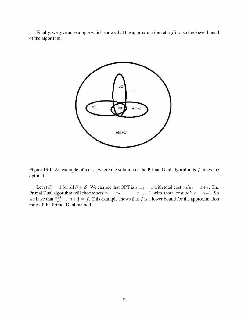
Finally, we give an example which shows that the approximation ratio f is also the lower boundof the algorithm.
Figure 13.1: An example of a case where the solution of the Primal Dual algorithm is f times theoptimal
Let c(S) = 1 for all S ∈ S. We can see that OPT is xn+1 = 1 with total cost value = 1+ε. ThePrimal Dual algorithm will choose sets x1 = x2 = ... = xn+1=1, with a total cost value = n+1. Sowe have that n+1
1+ε→ n+1 = f . This example shows that f is a lower bound for the approximation
ratio of the Primal Dual method.
75