1

Lecture 9: Panel Data Model (Chapter 14, Wooldridge Textbook)

2

Panel Data

• Panel data is obtained by observing the same person, firm, county, etc over several periods.

• Unlike the pooled cross sections, the observations for the same cross section unit (panel,entity, cluster) in general are dependent. Thus cluster-robust statistics that account forcorrelation within panel should be used.

3

Organizing Panel Data

• It is important to have an ID variable that distinguishes one entity from others, such aspatient ID, firm ID and county name.

• The observations for the same panel (over several periods) should be adjacent. This iscalled long form required by Stata command xtreg.

• The data for the minimum wage paper is wide form. Stata command

reshape

can be used to transform the wide form to the long form.

4

Panel Data and Causality

• Panel data can be used to control for time invariant unobserved heterogeneity, and thereforeis widely used for causality research.

• By contrast, cross sectional data cannot control for time invariant unobserved heterogeneity,so may suffer bigger omitted variable bias than panel data.

• The idea is simple. We take various forms of difference, and the time invariant unobservedheterogeneity is removed.

• Effectively, the panel data use the same panel as both treatment group and control group,and by invoking the before and after comparison, remove the time invariant omittedvariables. The limitation of panel data is that time varying omitted variables are stillpresent. But overall, the omitted variable bias gets smaller than cross sectional data.

5

Unobserved Effect Panel Data Model

• Consider a two-period unobserved effect model

yit = β0 +δ0dt +β1xit +ai + eit (1)

• The subscript i indexes panels, while t indexes periods.

• ai is time constant unobserved heterogeneity. eit is the idiosyncratic error, or time-varyingunobserved heterogeneity. ai + eit is the composite error term.

• dt is time dummy, so is panel constant and time varying; you can think of ai as paneldummy, so is time constant and panel varying.

6

Endogeneity

• The main reason to use panel data is to correct for the endogeneity caused by unobservedtime constant effect, i.e.,

cov(xit ,ai) = 0 (2)

• Given that nonzero covariance, the pooled OLS estimator applied to (1) is inconsistent.

7

First Difference (FD) Estimator I

• The repeated observations for the same panel make it possible to remove ai via differencing

• First write down the regression for period 2 and period 1 explicitly as

yit=2 = β0 +δ0 ∗1+β1xit=2 +ai + eit=2 (3)

yit=1 = β0 +δ0 ∗0+β1xit=1 +ai + eit=1 (4)

Now it is clear that ai can be removed by subtracting the second equation from the first one.

8

First Difference (FD) Estimator II

• So we compute the first time difference for each panel

∆yi = yi,t=2 − yi,t=1 (5)

∆xi = xi,t=2 − xi,t=1 (6)

∆ei = ei,t=2 − ei,t=1 (7)

• Finally, run the regression using the first-differened data, called first difference equation:

∆yi = δ0 +β1∆xi +∆ei (8)

Notice that both ai and β0 disappear. In general, differencing removes all time constantvariables (such as gender).

• OLS applied to the FD regression (8) yields the so called first-difference estimator. The FDestimator is consistent and has causal interpretation if the regressor in (8) is exogenous, i.e.,

E(∆xi,∆ei) = 0 (9)

9

Serial Correlation

• In general the error term in the difference regression (8), ∆ei, is negatively seriallycorrelated when eit is serially uncorrelated.

• For example, if data have three periods, then

E(∆ei,t∆ei,t−1) = E[(ei,t=3 − ei,t=2)(ei,t=2 − ei,t=1)] =−σ2e < 0

• So cluster-robust statistics should be used.

10

Diminishing Variation

Typically, the variation in the differenced independent variable is much smaller than thevariation in the original independent variable. Thus imprecise estimate can be expected from FDestimator. Like the IV estimator, here we face the same tradeoff of efficiency versusunbiasedness.

11

STATA Command

The STATA command to get the time differenced data is

by panelid: gen dy = y[_n]-y[_n-1]

by panelid: gen dx = x[_n]-x[_n-1]

This will produce missing value for the first observation of each entity. The “by panelid”part is important. Without that part you will get overall difference, which is meaningless for ourpurpose.

12

FD Estimator can be used to control for time-constant unobservedheterogeneity. FD estimator cannot be used when the regressor of interestis time-constant. FD estimator is imprecise when the regressor changeslittle over time.

13

Fixed Effect (FE) Estimator I

For concreteness let t = (1,2,3) in the following causal model

yit = β0 +δ1d1t +δ2d2t +β1xit +ai + eit (10)

Note that there are two time-dummies in (10) because there are three periods.

d1t =

1, period 1;

0, period 2 3.(11)

d2t =

1, period 2;

0, period 1 3.(12)

so period 3 is the base period.

14

Fixed Effect (FE) Estimator II

Averaging (10) across i leads to the so called between regression

yi = β0 +δ1d1t +δ2d2t +β1xi +ai + ei (13)

where the time averages are

yi =13

3

∑t=1

yit (14)

xi =13

3

∑t=1

xit (15)

ei =13

3

∑t=1

eit (16)

The average of ai is itself since it is time-invariant.

15

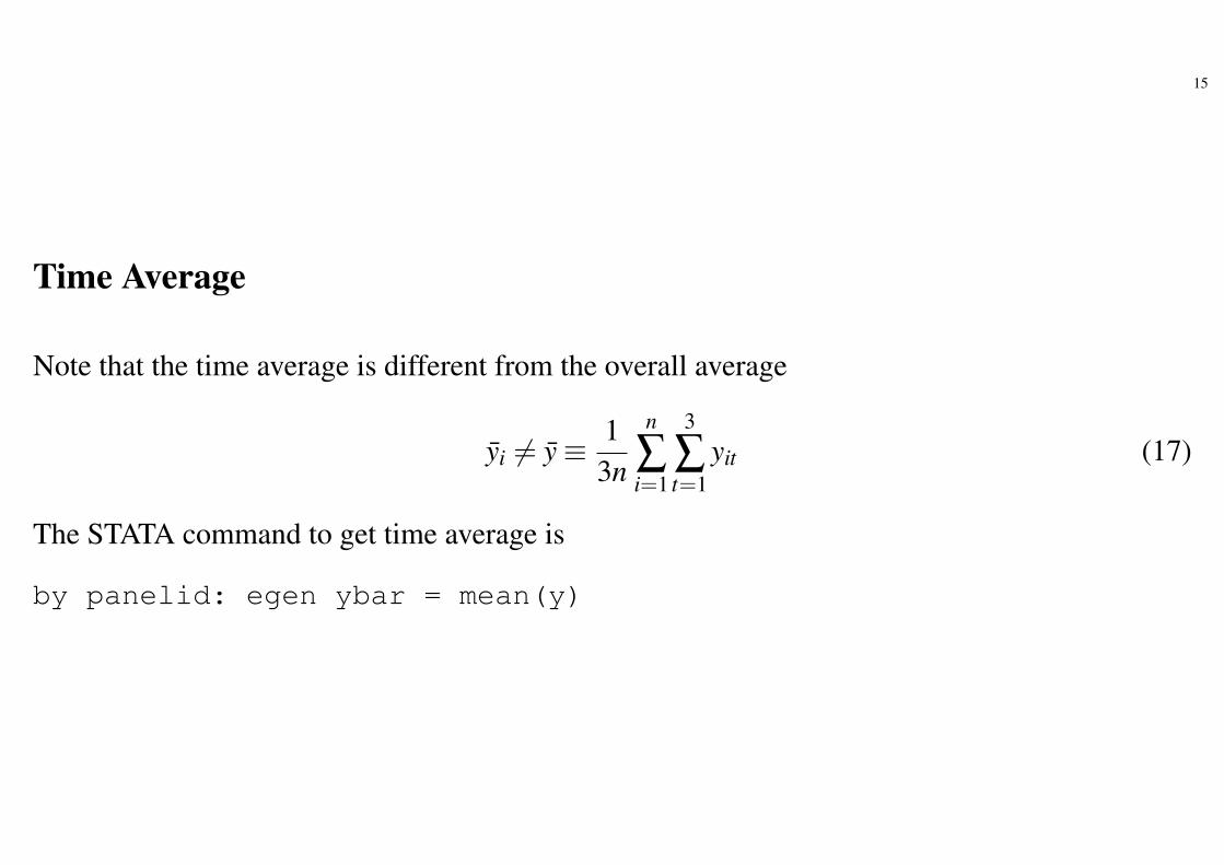
Time Average

Note that the time average is different from the overall average

yi = y ≡ 13n

n

∑i=1

3

∑t=1

yit (17)

The STATA command to get time average is

by panelid: egen ybar = mean(y)

16

Between Regression

OLS estimator applied to the between regression is inconsistent since

cov(xiai) =1n ∑

tcov(xitai) = 0,

see (2). However later we will use between equation to get estimate for the panel dummy ai.

17

Fixed Effect (FE) Estimator III

Subtracting the between regression (13) from (10) leads to the so called within regression

ydemeanit = δ1d1demeant +δ2d2demeant +β1xdemeanit + edemeanit (18)

where

ydemeanit = yit − yi (19)

xdemeanit = xit − xi (20)

edemeanit = eit − ei (21)

Note ai is removed. Finally OLS applied to the within regression (18) is the FE estimator.

18

Dummy Variable Regression

The FE estimator can be alternatively obtained from a dummy variable regression

yit = β0 +δ1d1t +δ2d2t +n−1

∑j=1

a jc j +β1xit +uit (22)

where c j is the dummy variable for the j-th cross unit:

c j =

1, cross unit j;

0, other cross units.(23)

and a j is its coefficient.The STATA command is

areg y x, absorb(panelid)

19

Frisch-Waugh Theorem

Essentially the dummy variable regression treats ai in (10) as entity-specific intercept terms. TheFrisch-Waugh theorem indicates that β1 in the dummy variable regression (22) is numericallyequivalent to the FE estimator obtained from the within regression (18).

20

STATA Command

The STATA command

xtreg y x, fe vce(robust)

produces the FE estimator along with cluster-robust standard error. If you include a timeconstant independent variable such as gender, it will be dropped.

21

Fixed Effect

You can estimate the fixed effect ai by replacing coefficient with its FE estimates in the betweenregression

ai = yi − β0 − δ1d1t − δ2d2t − β1xi (24)

STATA also reports the F test for the joint significance of fixed effects:

H0 : a1 = a2 = . . .= an−1 = 0 (25)

22

Remarks

• FE estimator cannot be used when the regressor of interest xit is time-invariant (such asgender).

• Cluster Robust Standard Error should be used in the within regression (18) since edemeanit isserially correlated.

• FE and FD estimators are inconsistent when E(xiteit) = 0 in the main model (10). In thatcase, IV variable is needed to completely resolve the endogeneity issue.

23

Three Questions

• Q: Why do we need time dummy?

• A: The time dummy d1t and d2t in (10) can control for time varying but panel constantunobserved effect. Example is national trend. It affects every panel and evolves over time.

• Q : Why do we need panel dummy?

• The panel dummy c j in (22) can control for panel varying but time constant unobservedeffect. Example is ability. It varies across persons but remains unchanged over time.

• Q: What if there are time-varying omitted variables?

• A: IV is still needed if there is time-varying omitted variable. Nevertheless finding IV forthe within regression is easier than finding IV for the original regression (Why?)

24

Panel data model is useful when the omitted variable is time-invariant.Panel data model cannot be used when the key regressor is time-invariant.IV Estimator applied to the Within Regression should be considered whenthe omitted variable is time-varying.