Lecture 9 GxE Mixed Models - University of...

Lecture 9 GxE Mixed Models

Lucia GutierrezTucson Winter Institute

1

Genotypic Means

GENOTYPIC MEANS:

The environment includes non-genetic factors that affect the phenotype, and usually has a large influence on quantitative traits. o Micro-environment. Environment of a single plant. Need to be

controlled with experimental design.o Macro-environment. Environment associated to a location

and time. GxE is the norm and not the exception in plants. Therefore defining the target environments is a crucial part in plant breeding, both for variance component estimation and identyfing superior genotypes.

ijkijjiijk GEEGy ε+++=

Bernardo 20102

Outline

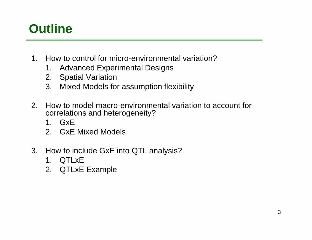
1. How to control for micro-environmental variation? 1. Advanced Experimental Designs2. Spatial Variation3. Mixed Models for assumption flexibility

2. How to model macro-environmental variation to account for correlations and heterogeneity?1. GxE2. GxE Mixed Models

3. How to include GxE into QTL analysis?1. QTLxE2. QTLxE Example

3

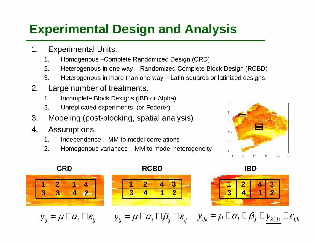
Experimental Design and Analysis1. Experimental Units.

1. Homogenous –Complete Randomized Design (CRD)2. Heterogenous in one way – Randomized Complete Block Design (RCBD)3. Heterogenous in more than one way – Latin squares or latinized designs.

2. Large number of treatments.1. Incomplete Block Designs (IBD or Alpha)2. Unreplicated experiments (or Federer)

3. Modeling (post-blocking, spatial analysis)4. Assumptions,

1. Independence – MM to model correlations2. Homogenous variances – MM to model heterogeneity

CRD RCBD IBD

13

12

243

4 14

42

213

3 14

42

213

3

ijiijy εαµ ++= ijjiijy εβαµ +++= 4ijkjkjiijky εγβαµ ++++= )(

AssumptionsClassical models are based on some limiting assumptions: Errors are independent random variables with normal distribution and homogenous variances.

DEPENDENCIES• Design factors impose restrictions on randomizations that induce

correlations (i.e. plots within a block are more similar to each other than toplots on a different block). If correlations exist, they should be included in themodel to make valid inferences.

• Genotypes may be related imposing a correlation.• Field heterogeneity also induces correlations. • There might be a correlation between environments.

NON-HOMOGENOUS VARIANCES• Both, genetic and environmental variances are affected by the environment

(i.e. they are properties of the population). Therefore, heterogenousvariances are common in field experiments.

5

Mixed Models in Field ExperimentsMixed models are more flexible: correlations and heterogenousvariances can be modeled.

FIXED EFFECTS• inference is about specific treatments• all levels of a fixed factor are included in the experiment• interest in testing differences in means between treatments• need for identification constraints (sum to zero, cornerstone)

RANDOM EFFECTS• inference is about a population of treatments• testing the population variance of a treatment• assumed to have a distribution, ti ~ N(0, σt

2)• structuring of variance-covariance, imposing correlations• prediction from random effects provides best estimate of treatment

rankings (BLUPs) 6

Fixed Effects vs. Random Effects

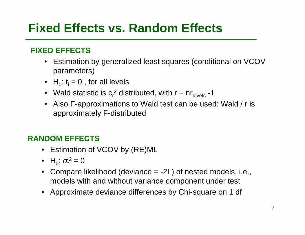
FIXED EFFECTS• Estimation by generalized least squares (conditional on VCOV

parameters)• H0: ti = 0 , for all levels• Wald statistic is cr

2 distributed, with r = nrlevels -1• Also F-approximations to Wald test can be used: Wald / r is

approximately F-distributed

RANDOM EFFECTS• Estimation of VCOV by (RE)ML • H0: σt

2 = 0• Compare likelihood (deviance = -2L) of nested models, i.e.,

models with and without variance component under test• Approximate deviance differences by Chi-square on 1 df

7

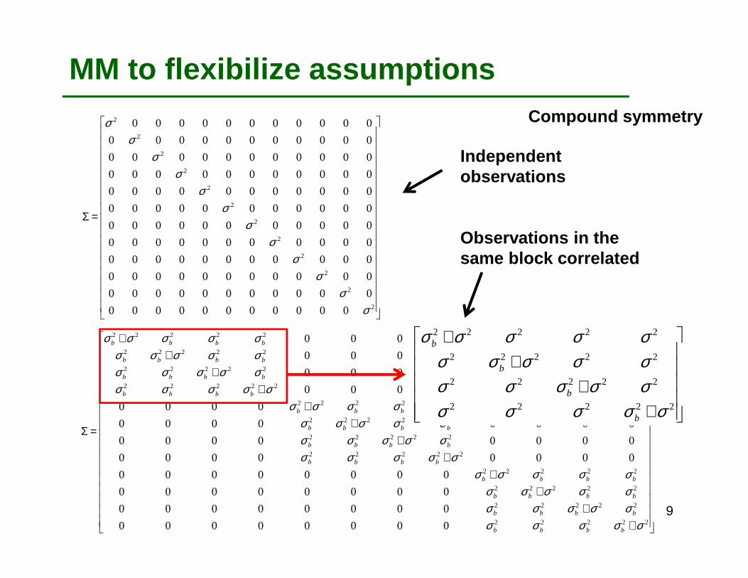
MM to flexibilize assumptions

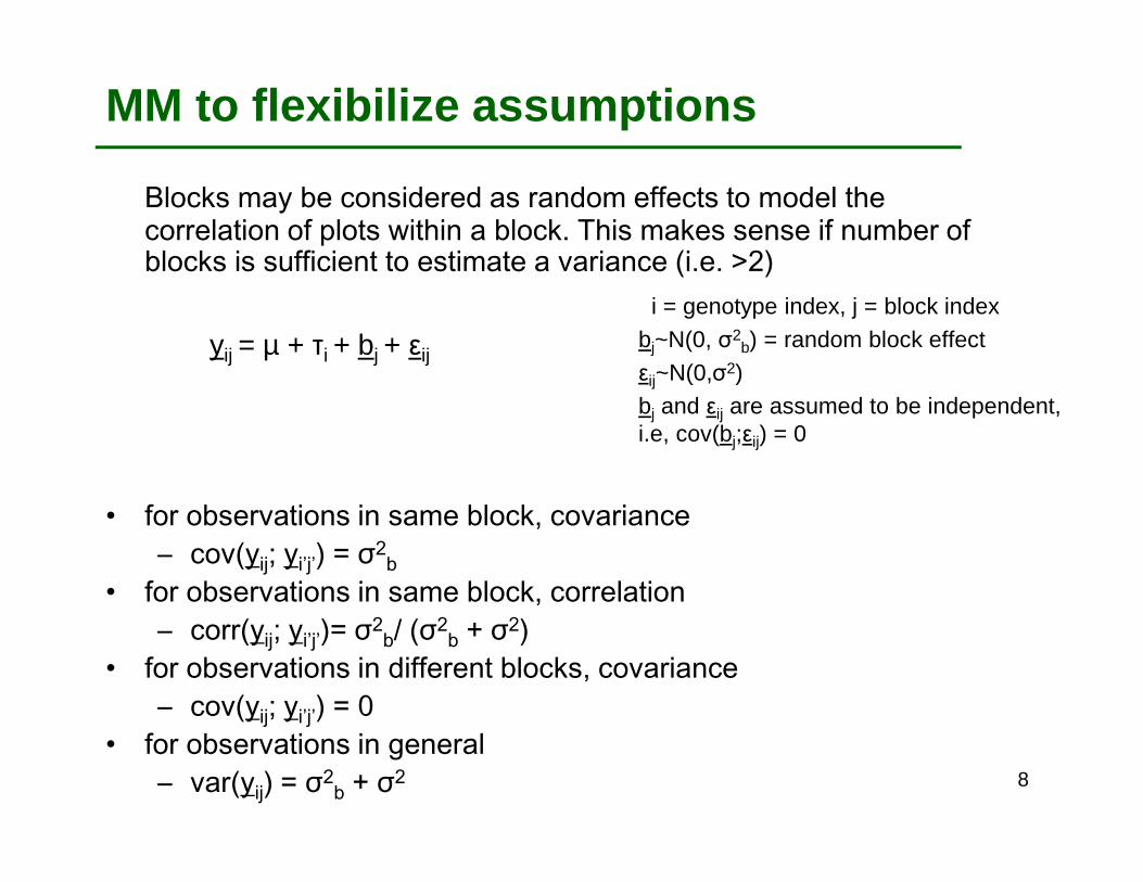
Blocks may be considered as random effects to model the correlation of plots within a block. This makes sense if number of blocks is sufficient to estimate a variance (i.e. >2)

yij = µ + τi + bj + εij

• for observations in same block, covariance– cov(yij; yi’j’) = σ2

b• for observations in same block, correlation

– corr(yij; yi’j’)= σ2b/ (σ2

b + σ2) • for observations in different blocks, covariance

– cov(yij; yi’j’) = 0 • for observations in general

– var(yij) = σ2b + σ2

i = genotype index, j = block indexbj~N(0, σ2

b) = random block effectεij~N(0,σ2) bj and εij are assumed to be independent, i.e, cov(bj;εij) = 0

8

MM to flexibilize assumptions

=Σ

2

2

2

2

2

2

2

2

2

2

2

2

00000000000

00000000000

00000000000

00000000000

00000000000

00000000000

00000000000

00000000000

00000000000

00000000000

00000000000

00000000000

σσ

σσ

σσ

σσ

σσ

σσ

++

++

++

++

++

++

=Σ

22222

22222

22222

22222

22222

22222

22222

22222

22222

22222

22222

22222

00000000

00000000

00000000

00000000

00000000

00000000

00000000

00000000

00000000

00000000

00000000

00000000

σσσσσσσσσσσσσσσσσσσσ



bbbb

bbbb

bbbb

bbbb

bbbb

bbbb

bbbb

bbbb

bbbb

bbbb

bbbb

bbbb

Independent observations

Observations in the same block correlated

++

++

22222

22222

22222

22222


b

b

b

b

Compound symmetry

9

Number of treatments

HOW TO DEAL WITH HIGH NUMBER OF TREATMENTS?

1. STRATIFICATION: Group genotypes with similar characteristics(maturity, color, family), compare within groups. NO BETWEEN GROUP COMPARISONS.

2. PRODUCE HOMOGENOUS EXPERIMENTAL UNITS: Make everyeffort to homogenize experimental area (look for soil similarity, fieldconditions to reduce variation, choose seeds of similar vigor).

3. USE REPEATED CHECKS: You may use checks in a systematicway to control or model soil heterogeneity.

4. EXPERIMENTAL DESIGN WITH SPATIAL CONSIDERATIONS. Use experimental designs that include a large number of treatmentswhile controling variability (i.e. alpha designs, unrep, etc.).

10

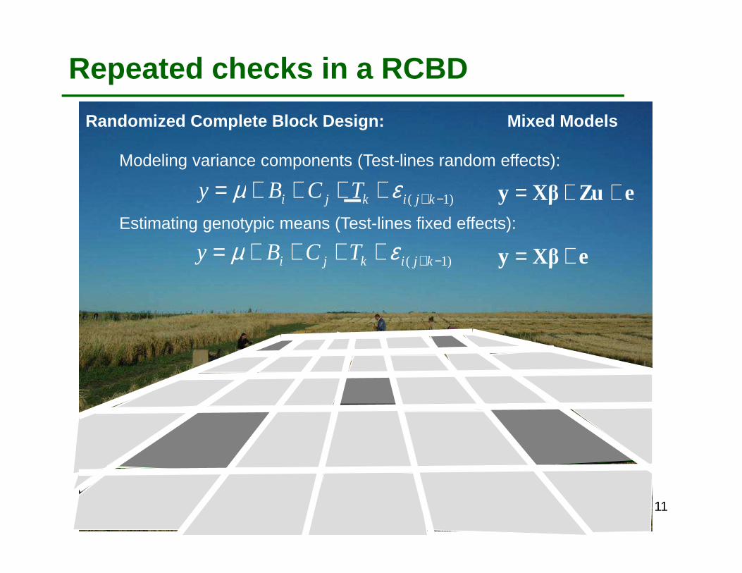
Repeated checks in a RCBD

C C

C

C

C

Randomized Complete Block Design:

)1( −+++++= kjikji TCBy εµModeling variance components (Test-lines random effects):

Estimating genotypic means (Test-lines fixed effects):

)1( −+++++= kjikji TCBy εµ eXβy +=

eZuXβy ++=

Mixed Models

11

Advanced Designs: Alpha Designs

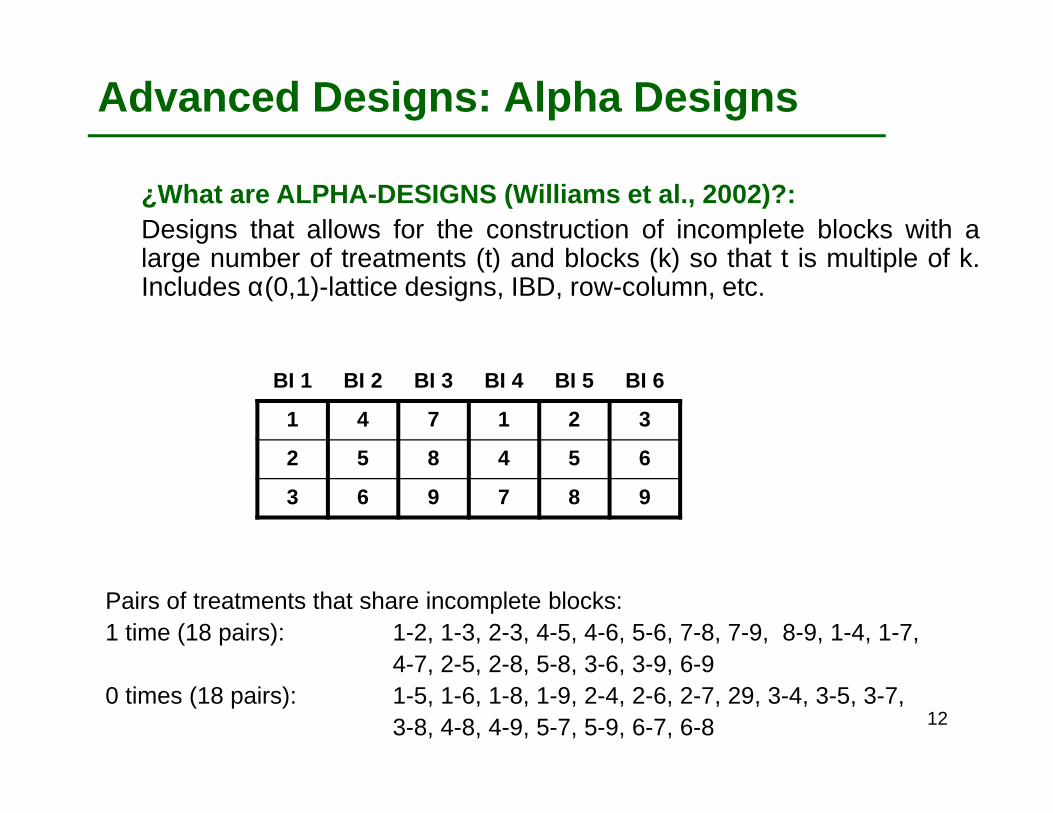
¿What are ALPHA-DESIGNS (Williams et al., 2002)?:Designs that allows for the construction of incomplete blocks with alarge number of treatments (t) and blocks (k) so that t is multiple of k.Includes α(0,1)-lattice designs, IBD, row-column, etc.

Pairs of treatments that share incomplete blocks:1 time (18 pairs): 1-2, 1-3, 2-3, 4-5, 4-6, 5-6, 7-8, 7-9, 8-9, 1-4, 1-7,

4-7, 2-5, 2-8, 5-8, 3-6, 3-9, 6-90 times (18 pairs): 1-5, 1-6, 1-8, 1-9, 2-4, 2-6, 2-7, 29, 3-4, 3-5, 3-7,

3-8, 4-8, 4-9, 5-7, 5-9, 6-7, 6-8

BI 1 BI 2 BI 3 BI 4 BI 5 BI 6

1 4 7 1 2 3

2 5 8 4 5 6

3 6 9 7 8 9

12

Advanced Designs

Replicate 1 Replicate 2Block 1 2 3 1 2 3

1 4 7 1 2 32 5 8 4 5 63 6 9 7 8 9

Replicate 1 Replicate 2Block 1 2 3 1 2 3

1 4 7 1 5 42 5 8 2 8 63 6 9 3 9 7

Which is the best design?

Two possible arrangements for an incomplete block design with r = 2, v = 9 and k = 3

13

Advanced Designs

DESIGN• Block 1: ABC; Block 2: ABD; Block 3: ACD; Block 4: BCD• Coincidence of treatments inside incomplete blocks = 2

COMPARISONS• Direct:

• For A-B: Block 1 and 2: A-B• Indirect:

• For A-B: (Block 1, A-C) – (Block 4, B-C) = A-B• Block Totals:

• Sum Block 3 – Sum Block 4 = (A+C+D) – (B+C+D) = A-B

14

Mixed Models in Advanced Designs

• Direct and indirect comparisons of treatment effects are combined in standard least squares, fixed effects, estimates = intra block estimates.

• Information on treatment differences from block totals becomes available only when blocks are taken random = inter block estimates.

• Combination of intra and inter block estimates for treatment differences weighing the pieces of information by their (inverse) variances is done automatically in a REML analysis

15

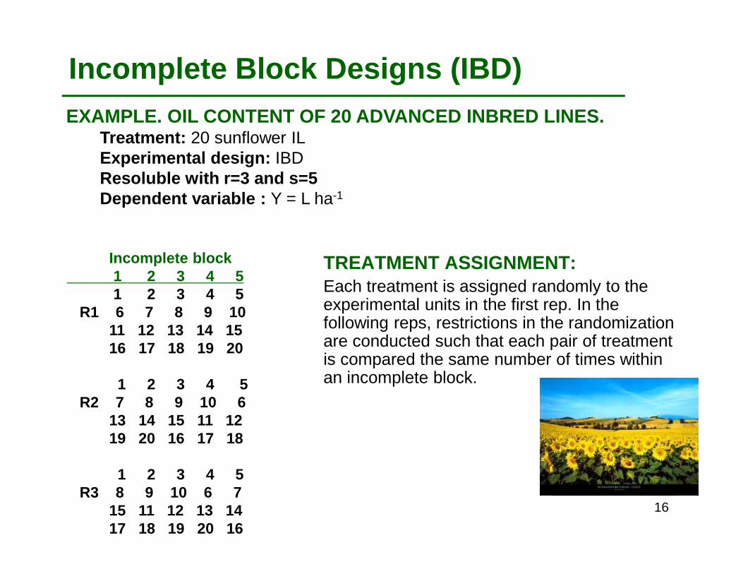
Incomplete Block Designs (IBD)EXAMPLE. OIL CONTENT OF 20 ADVANCED INBRED LINES.

Treatment: 20 sunflower ILExperimental design: IBDResoluble with r=3 and s=5Dependent variable : Y = L ha-1

Incomplete block1 2 3 4 51 2 3 4 5

R1 6 7 8 9 10 11 12 13 14 1516 17 18 19 20

1 2 3 4 5R2 7 8 9 10 6

13 14 15 11 1219 20 16 17 18

1 2 3 4 5R3 8 9 10 6 7

15 11 12 13 1417 18 19 20 16

TREATMENT ASSIGNMENT:Each treatment is assigned randomly to theexperimental units in the first rep. In thefollowing reps, restrictions in the randomizationare conducted such that each pair of treatmentis compared the same number of times withinan incomplete block.

16

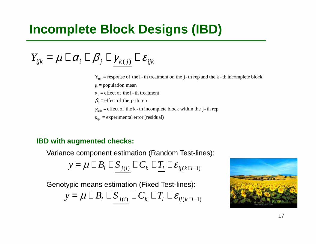
Incomplete Block Designs (IBD)

ijkjkjiijkY εγβαµ ++++= )(

IBD with augmented checks:

)1()( −++++++= lkijlkiji TCSBy εµVariance component estimation (Random Test-lines):

Genotypic means estimation (Fixed Test-lines):

)1()( −++++++= lkijlkiji TCSBy εµ

(residual)error alexperimentε

repth -j in theblock with incompleteth -k theofeffect

repth -j theofeffect

ntth treatme-i theofeffect α

mean populationµ

block incompleteth -k theand repth -j on thent th treatme-i theof responseY

ijk

k(j)

j

i

ijk

=

=

==

=

=

γβ

17

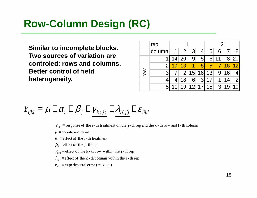
Row-Column Design (RC)

repcolumn 1 2 3 4 5 6 7 8

1 14 20 9 5 6 11 8 202 10 13 1 8 5 7 18 123 7 2 15 16 13 9 16 44 4 18 6 3 17 1 14 25 11 19 12 17 15 3 19 10

row

1 2

ijkljljkjiijklY ελγβαµ +++++= )()(

Similar to incomplete blocks. Two sources of variation are controled: rows and columns. Better control of fieldheterogeneity.


repth -j hin thecolumn witth -k theofeffect

repth -j e within throwth -k theofeffect


ntth treatme-i theofeffect α

mean populationµ

columnth -l and rowth -k theand repth -j on thent th treatme-i theof responseY

ijkl

l(j)

k(j)

j

i

ijkl

=

=

=

==

=

=

λγβ

18

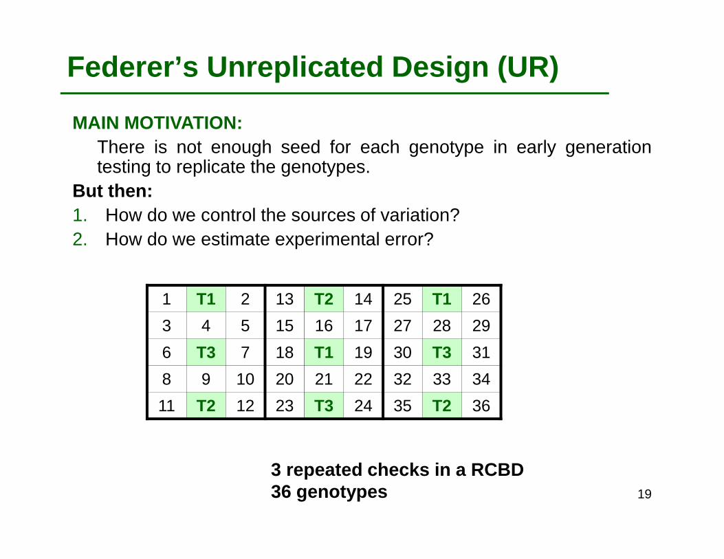
Federer’s Unreplicated Design (UR)

MAIN MOTIVATION:There is not enough seed for each genotype in early generationtesting to replicate the genotypes.

But then:1. How do we control the sources of variation?2. How do we estimate experimental error?

T1 T2 T1

T3 T1 T3

T2 T3 T2

1 T1 2 13 T2 14 25 T1 26

3 4 5 15 16 17 27 28 29

6 T3 7 18 T1 19 30 T3 31

8 9 10 20 21 22 32 33 34

11 T2 12 23 T3 24 35 T2 36

3 repeated checks in a RCBD36 genotypes 19

Federer’s Unreplicated Designs (UR)

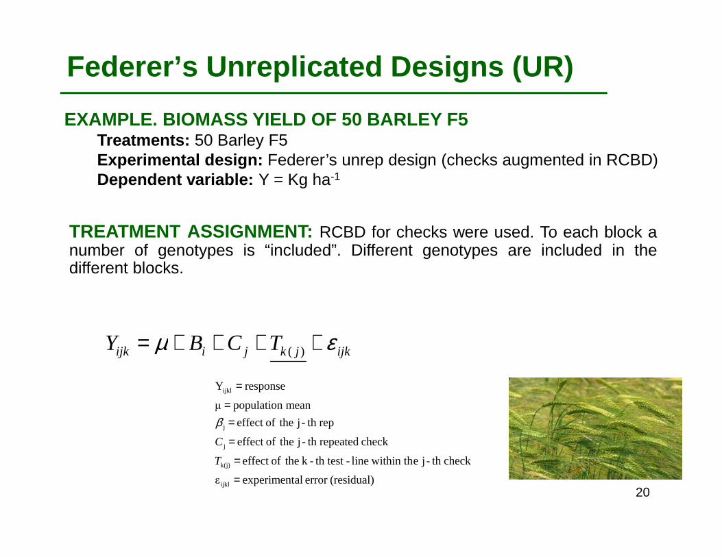
TREATMENT ASSIGNMENT: RCBD for checks were used. To each block anumber of genotypes is “included”. Different genotypes are included in thedifferent blocks.

EXAMPLE. BIOMASS YIELD OF 50 BARLEY F5Treatments: 50 Barley F5Experimental design: Federer’s unrep design (checks augmented in RCBD)Dependent variable: Y = Kg ha-1

ijkjkjiijk TCBY εµ ++++= )(


checkth -j e within thline-th test-k theofeffect

check repeatedth -j theofeffect


mean populationµ

responseY

ijkl

k(j)

j

j

ijkl

=

=

=

==

=

T

C

β

20

Spatial Modeling

VCOV for individual trials can be modeled as a product of a decaying correlation (for example: AR1) in row direction and another decaying correlation (for example: AR1) in column direction.

Spatial modeling of VCOV can be additional to blocks, or substitute of blocks (but then be careful).

Experimental design vs. post-blocking.

In mixed models with random blocks, all plots within a block are equally correlated, but between blocks plots are uncorrelated. It is more realistic that the correlation between plots decays with the distance between them.

1

1

1

1

23

2

2

32

ρρρρρρρρρρρρ

21

Model Comparison

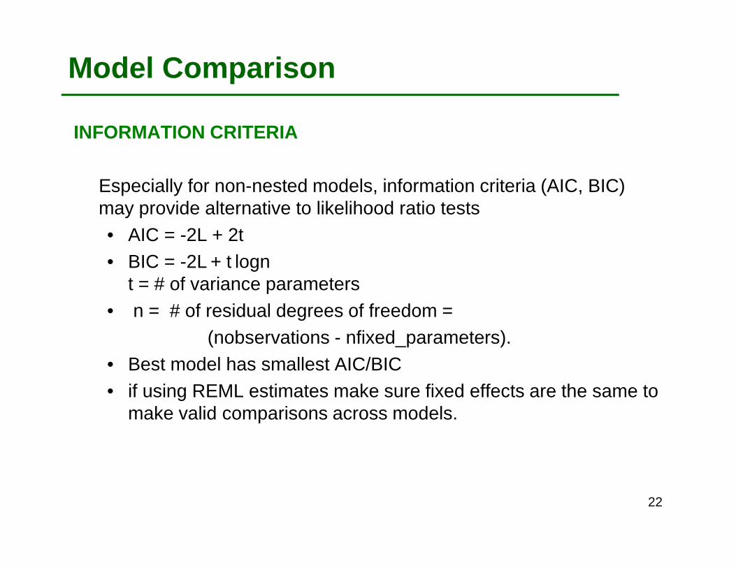
INFORMATION CRITERIA

Especially for non-nested models, information criteria (AIC, BIC) may provide alternative to likelihood ratio tests• AIC = -2L + 2t• BIC = -2L + t logn

t = # of variance parameters• n = # of residual degrees of freedom =

(nobservations - nfixed_parameters).• Best model has smallest AIC/BIC • if using REML estimates make sure fixed effects are the same to

make valid comparisons across models.

22

Why using Mixed Models ?

• Greater flexibility in modeling variance-covariance structure/ dependencies between observations.

• Accounting for heterogeneity of variance and correlation .

• For many situations linear mixed models provide a more natural way of modeling than standard linear models.

• Recovery of (inter-block) information.

• Shrinkage prediction of effects (BLUPs), which is of importance in genetics.

• Allows modeling of dependencies for spatial & temporal (blocking) and genetic reasons.

23

Genotype by Environment Interaction

Genotype1 Genotype 2 Genotype 1 Genotype 2

ENV 1 ENV 2

E1 E2

G2

G1

R

24

E1 E2


G2

G1

RG2

G1

R

G2

G1

R

E1 E2

G2

G1

R

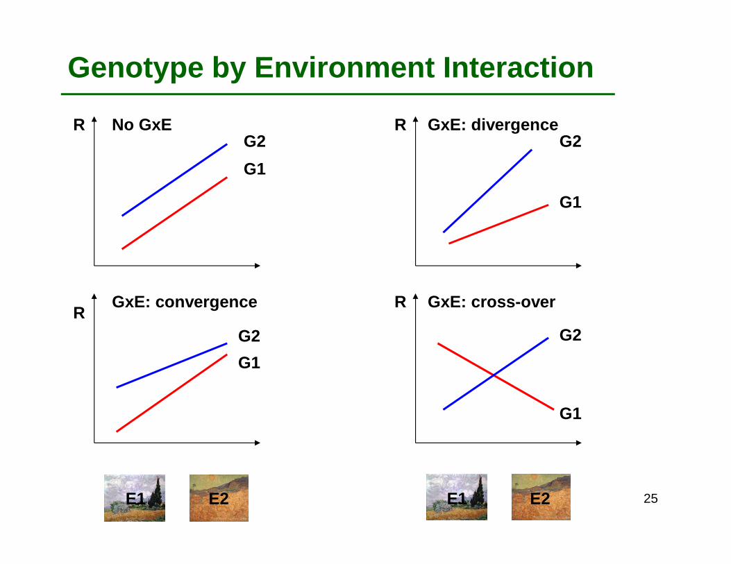
No GxE GxE: divergence

GxE: convergence GxE: cross-over

E1 E2 25


G2

G1

R

E1 E2

G2

G1

R

E1 E2

GxE: divergenceGxE: convergence

With both divergence and convergence, it is easy to make predictions because there is no cross-over interaction. G2 is the best genotype in all the environment. However, there is heterogeneity of variance that needs to be taken into account in models for proper estimation.

26


E1 E2

G2

G1

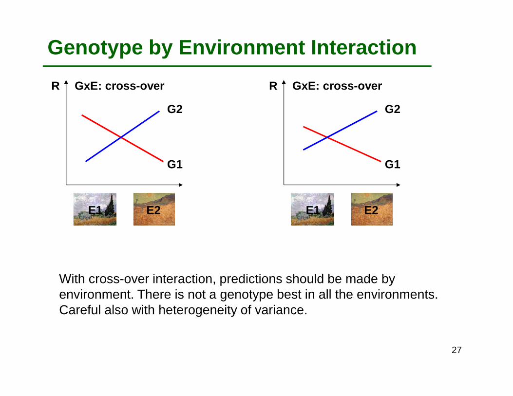
R GxE: cross-over

E1 E2

G2

G1

R GxE: cross-over

With cross-over interaction, predictions should be made by environment. There is not a genotype best in all the environments. Careful also with heterogeneity of variance.

27


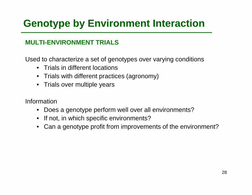
MULTI-ENVIRONMENT TRIALS

Used to characterize a set of genotypes over varying conditions• Trials in different locations• Trials with different practices (agronomy)• Trials over multiple years

Information• Does a genotype perform well over all environments?• If not, in which specific environments?• Can a genotype profit from improvements of the environment?

28

ONE-STAGE ANALYSIS

Analyze field-plot data and model GxE simultaneously. Need information from experimental design and replications.

TWO-STAGES ANALYSIS

Multiple environments

ijkijjkjiijk GEDEGP εµ +++++= )(

First stage: analysis per trial• Quality control (assumptions/outliers/etc)• Obtain predictions per genotype

Second stage: use the genotype by environment table of predictions• GxE analysis• QTLxE analysis

Trial 1 Trial 2 Trial n

GxE table of means

(predictions)

ijjiij GEEGP +++= µ 29

Multiple environments

The analysis of MET data aims at finding an adequate model for the phenotypic responses as a function of genetic and environmental factors � modelling the mean

• Reliable conclusions depends on an appropriate structure for the residual εij

• Assumption of independence of residuals between environments is highly unrealistic (in which case this assumption is valid?).

• A more realistic model assumes residuals coming from some multivariate normal distribution.

• Finding an appropriate structure for εij that reflects the heterogeneity of genetic variances and correlations a necessary first step towards reliable conclusions on µij

30

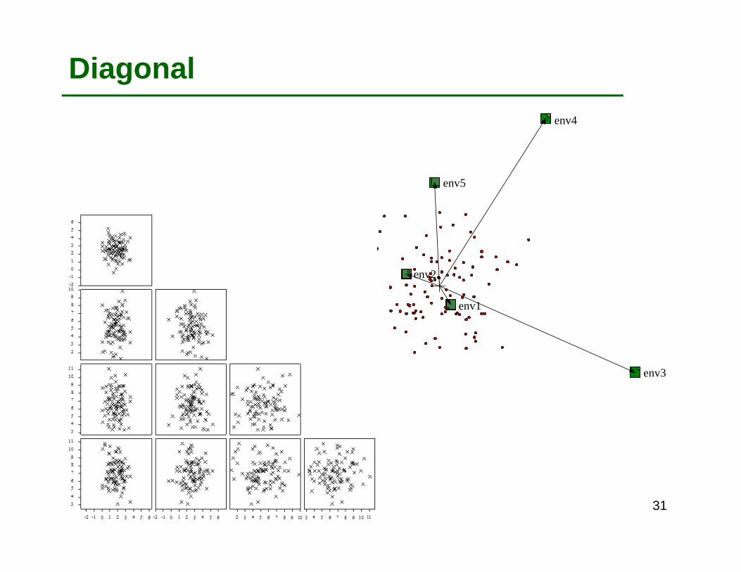
Diagonal

env1

env2

env3

env4

env5

31

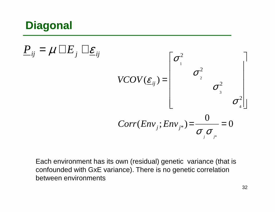
Diagonal

00

);(

)(

*

4

3

2

1

*

2

2

2

2

==

=

jj

jj

ij

EnvEnvCorr

VCOV

σσ

σσ

σσ

ε

Each environment has its own (residual) genetic variance (that is confounded with GxE variance). There is no genetic correlation between environments

ijjij EP εµ ++=

32

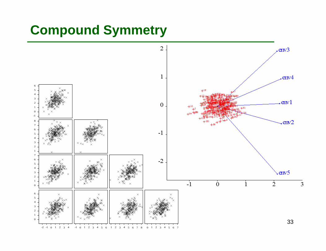
Compound Symmetry

6

5

4

3

2

7

1

5

0

314 73 52 31 10-1-2 6420

7

6

5

4

3

2

1

0

6262

8

7

5

6

1

5

4

3

2

1

44-1 08

6

5

3

4

3

2

1

0

-1

33

Compound Symmetry

22

2

2222

2

*

22222

2222

222

22

);(

)(

GEG

G

GEGGEG

Gjj

GEGGGG

GEGGG

GEGG

GEG

ij

EnvEnvCorr

VCOV

σσσ

σσσσσ

σσσσσσσσσ

σσσσσ

ε

+=

++=

++

++

=

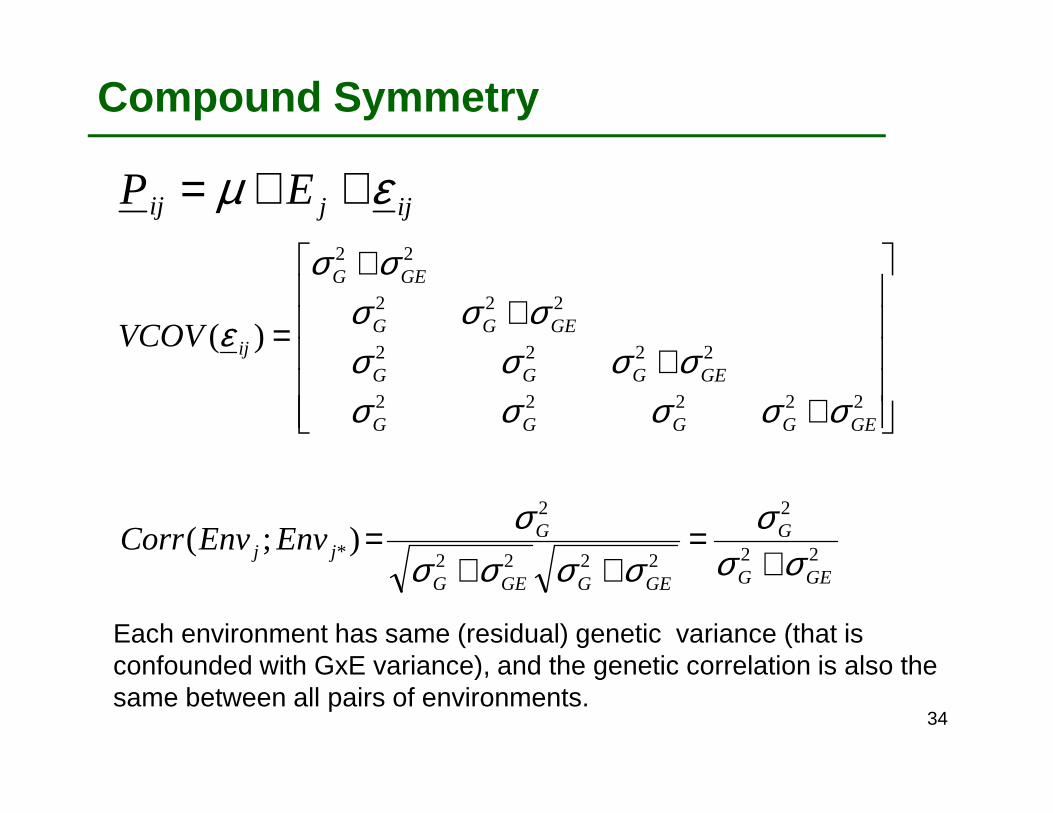
ijjij EP εµ ++=

Each environment has same (residual) genetic variance (that is confounded with GxE variance), and the genetic correlation is also the same between all pairs of environments.

34

Unstructured

env1env2

env3

env4

env5

35

Unstructured

*

**

24434241

233231

2221

21

);(

)(

jj

jjjj

ij

EnvEnvCorr

VCOV

σσσ

σσσσσσσ

σσσ

ε

=

=

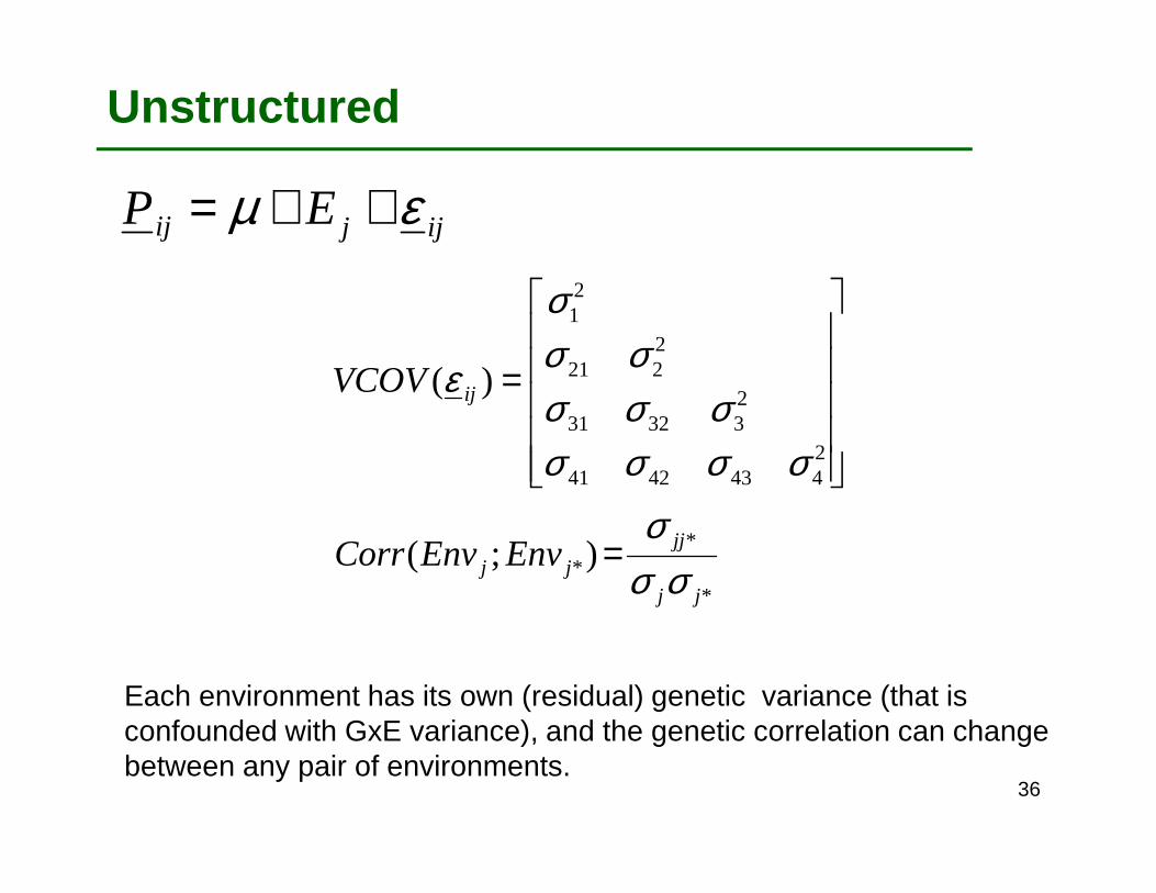
ijjij EP εµ ++=

Each environment has its own (residual) genetic variance (that is confounded with GxE variance), and the genetic correlation can change between any pair of environments.

36

Factor Analytic

jijijij

jijij

ijij

jij

zxE

xE

GE

E

βαµµαµµ

µµµµ

+++=

++=

++=

+=

))(();(

)(

2***

2

**

2444342414

23332313

222212

2111

jjjjjj

jjjj

ij

EnvEnvCorr

VCOV

δλλδλλ

λλδλλλλλλλλ

δλλλλλλδλλλλ

δλλ

ε

++=

++

++

=

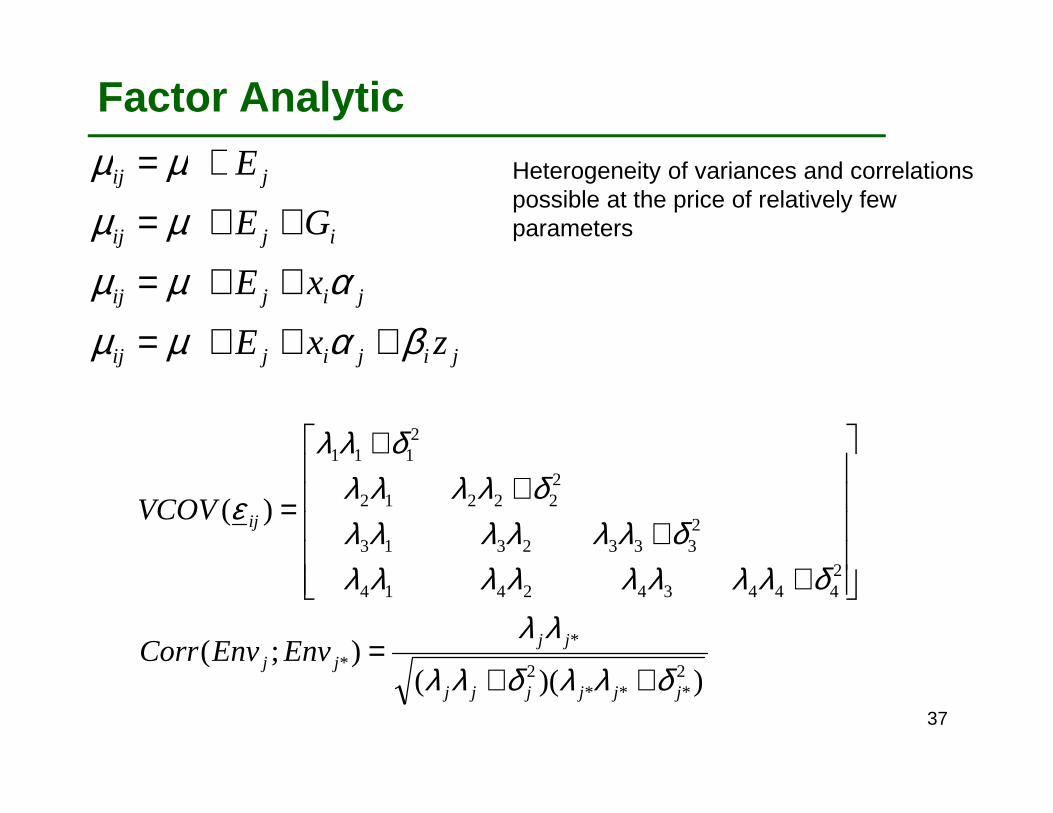
Heterogeneity of variances and correlations possible at the price of relatively few parameters

37

Finding a suitable model for the VCOV

• Use different summary statistics and diagnostic plots• Summary statistics per environment• Correlations between environments• Boxplots• Scatter plots• Biplots

• Fit different mixed models assuming different VCOV and compare the goodness of fit of them by some criterion (eg: AIC or BIC).

38

QTL x EWHY DO I NEED TO INCLUDE QTLxE?

o GxE is common in plants and multi-environment evaluation for Plant Breeding required.

o Modeling GxE to estimate means (BLUE) or predict BLUP is not enough?

o It is possible that a QTLxE interaction exists so that some markers are favorable in one environment but not in another one.

o Identifying general QTL and environment specific QTL is helpful in selecting best genotypes. Additionally, correct error terms should be used when QTL are being evaluated.

39

QTL x E

Genetic predictors(Genotypic covariables)

Grid of genomic positions

Markerscores

Environmental

covariables

Environments / time

Cov

aria

bles

Phenotypic data

GxE tableof meansG

enot

ypes

Marker Map

Geno-typic co-varia-

bles

Co-variables

Phenotypic data configuration

40

QTL x E

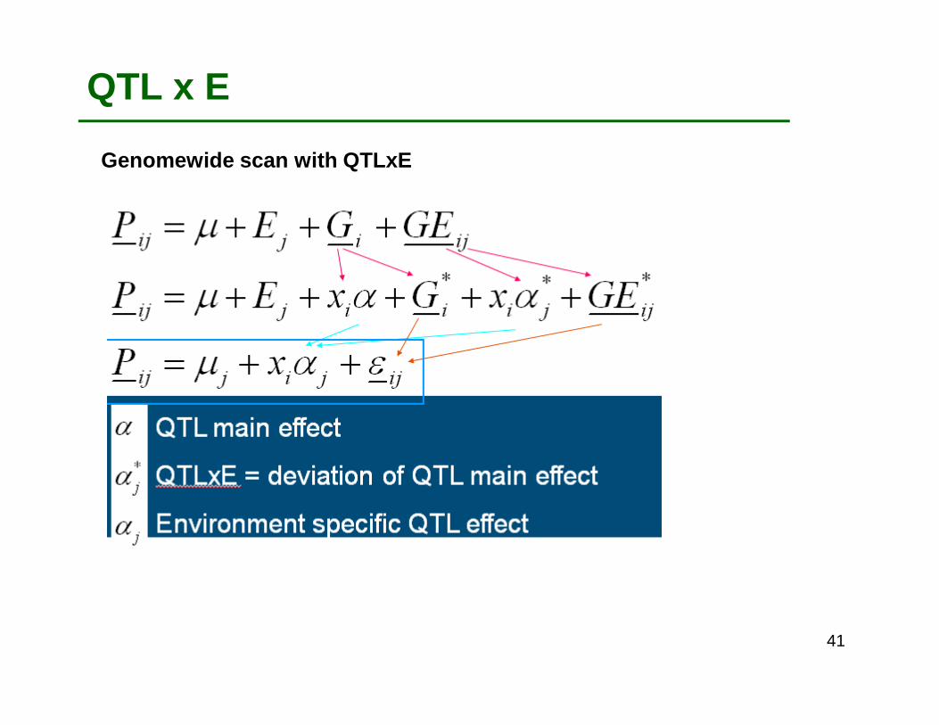
Genomewide scan with QTLxE

41

QTL x E

STEPS TO COMPLETE A QTLxE ANALYSIS

1. Identify appropriate model for GxE.

2. Use the appropriate model to test each genomic position for the presence of a QTL (MR/SIM).

3. Use candidate QTL as cofactors to re-scan de genome (CIM).

4. Adjust a final multi-QTL with backward elimination of candidate QTL. Estimate QTL effects.

42

Information needed

1. Molecular marker scores

2. Genetic map

3. Phenotypes

High throughput panels, controlled conditions, repeatable, cheap, automatic scoring.

More standard methods, small population sizes, consensus maps? Need some more development.

Crucial part, poor phenotypes means poor QTL mapping.

43

Phenotyping

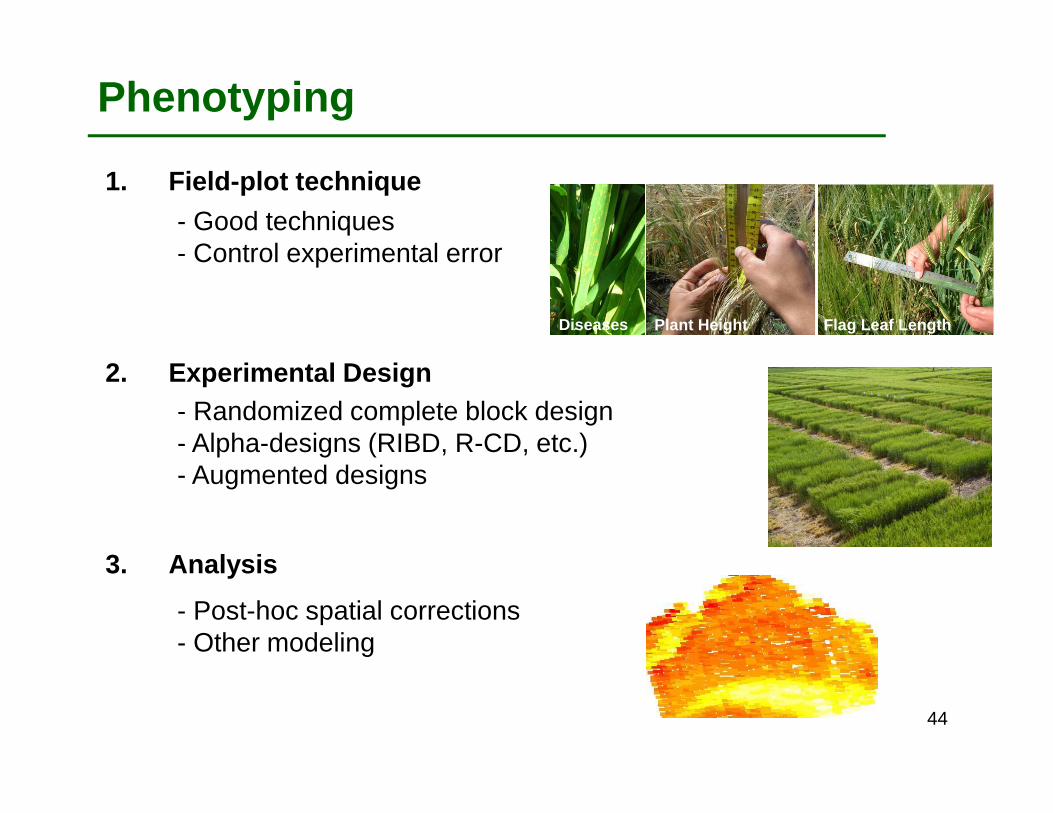
1. Field-plot technique

2. Experimental Design

3. Analysis

- Good techniques- Control experimental error

Plant Height Flag Leaf LengthDiseases

- Randomized complete block design- Alpha-designs (RIBD, R-CD, etc.)- Augmented designs

- Post-hoc spatial corrections- Other modeling

44

STRESS TRIALS1992 (Tlaltizapán, México)

– Well watered (WW)– Intermediate stress (IS)– Severe stress (SS)

1994 (Tlaltizapán, México)– Intermediate stress (IS)– Severe stress (SS)

1996 (Poza Rica, México)– Low Nitrogen (2 seasons)– High Nitrogen

Poza Rica

Tlaltizapán

Maize example (CIMMYT, MX)

Malosetti, 201145

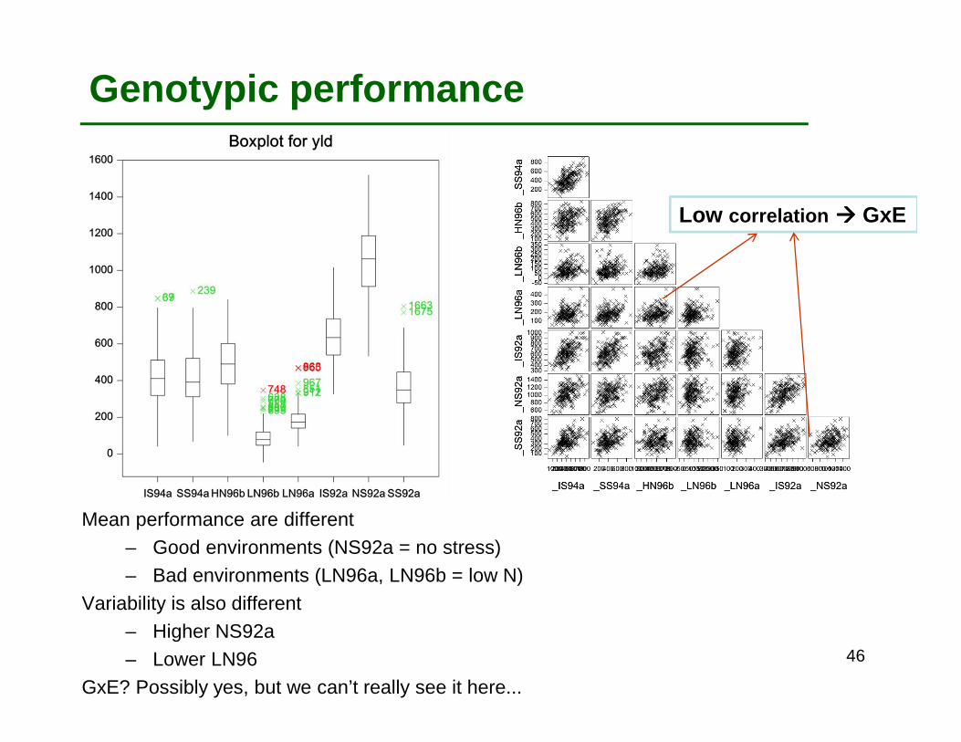
Mean performance are different – Good environments (NS92a = no stress)– Bad environments (LN96a, LN96b = low N)

Variability is also different– Higher NS92a– Lower LN96

GxE? Possibly yes, but we can’t really see it here...

Genotypic performance

Low correlation �� GxE

46

3 groups of environments

Genotypic performance

Best model for this data: Factor analytic

Model AIC SIC Deviance NParameters FA 17471 17524 17439 16 FA2 17455 17532 17409 23 OUTSIDE 17523 17554 17505 9 UNSTRUCTURED 17456 17577 17384 36 HCS 17692 17722 17674 9 CS 17918 17924 17914 2 DIAGONAL 17906 17933 17890 8 IDENTITY 18287 18290 18285 1 Best model: FA (on basis of criterion SIC) Malosetti, 2011

47

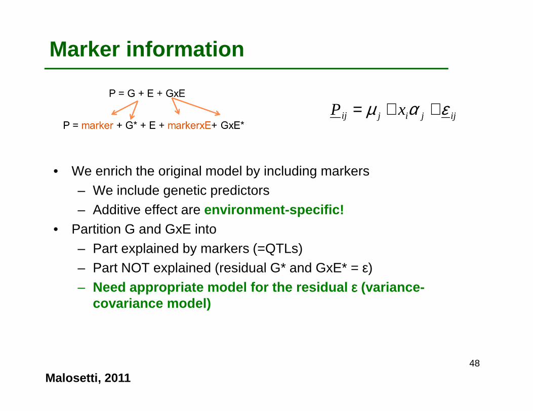
• We enrich the original model by including markers– We include genetic predictors– Additive effect are environment-specific!

• Partition G and GxE into– Part explained by markers (=QTLs)– Part NOT explained (residual G* and GxE* = ε)– Need appropriate model for the residual εεεε (variance-

covariance model)

ijjijij xP εαµ ++=

Marker information

Malosetti, 201148

Profile for environment specific QTLs

Positive effect P1 allele (dark/light blue)Positive effect P2 allele (red/yellow)

pos itive

5

ne gati ve

4

3

2

1

6

-log10(P

)

Color code for p-values of QTL effects

QTLxE (SIM; VCOC=FA)

Malosetti, 201149

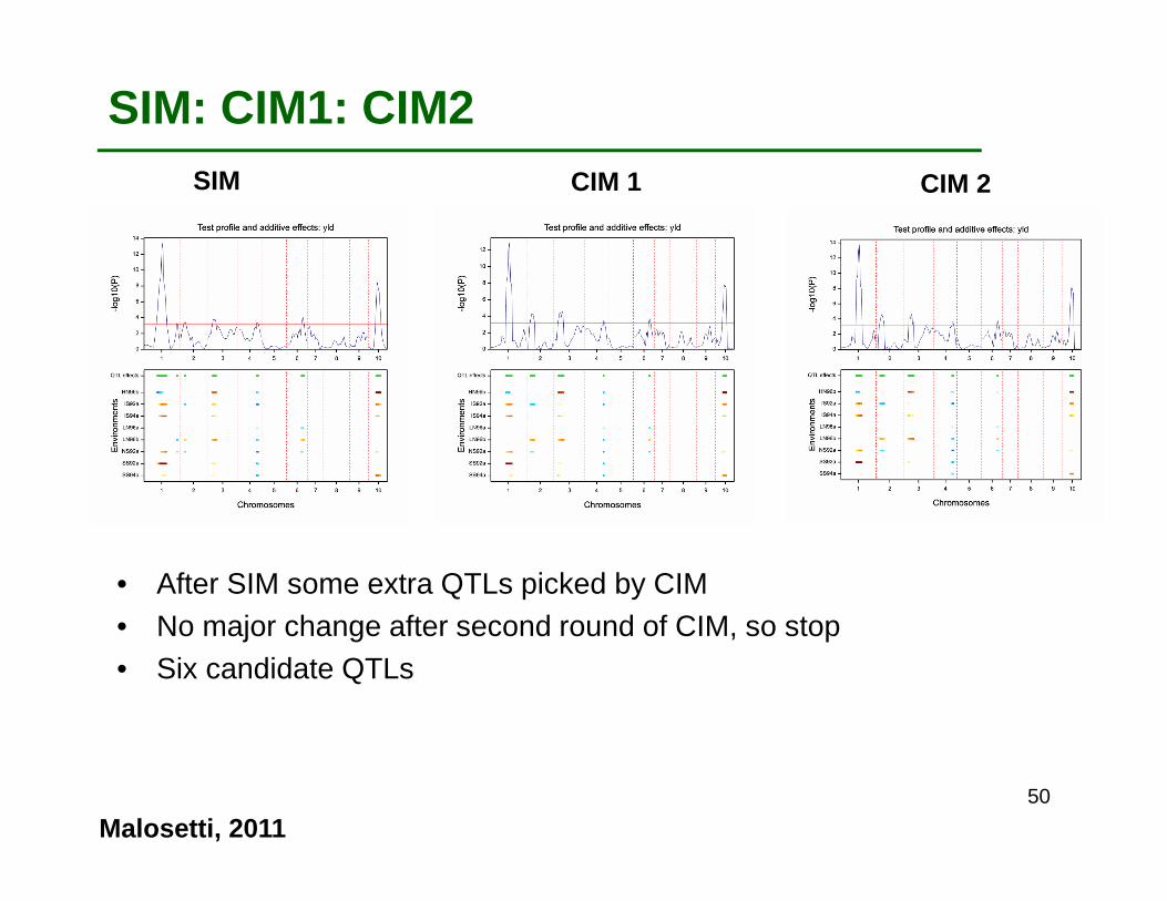
• After SIM some extra QTLs picked by CIM• No major change after second round of CIM, so stop• Six candidate QTLs

SIM CIM 1 CIM 2

SIM: CIM1: CIM2

Malosetti, 201150

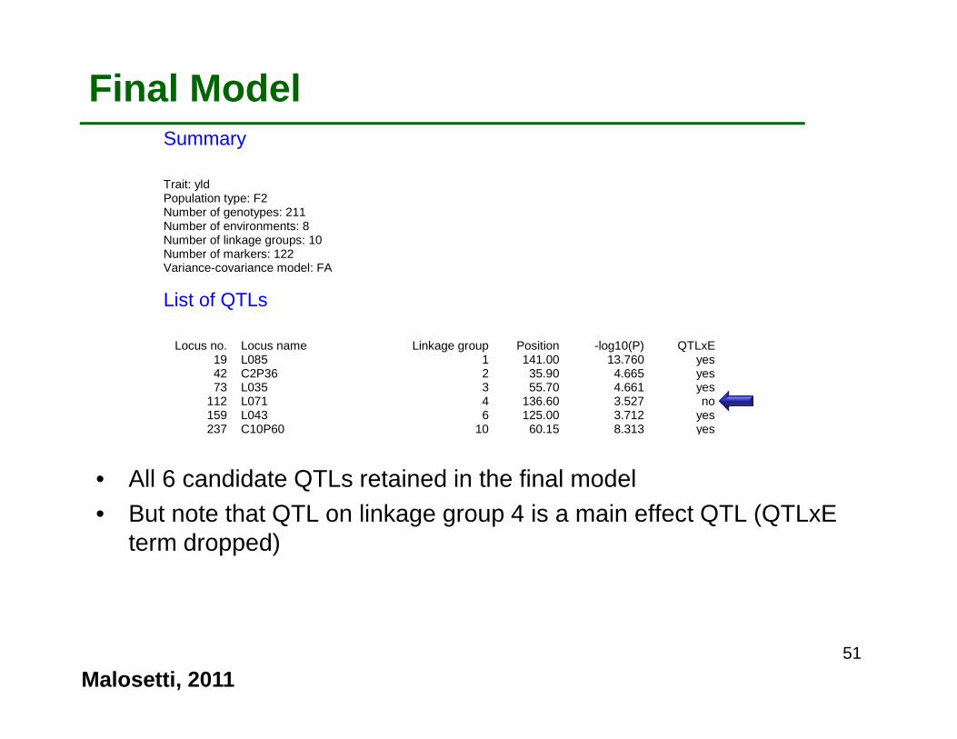
• All 6 candidate QTLs retained in the final model• But note that QTL on linkage group 4 is a main effect QTL (QTLxE

term dropped)

Summary Trait: yld Population type: F2 Number of genotypes: 211 Number of environments: 8 Number of linkage groups: 10 Number of markers: 122 Variance-covariance model: FA

List of QTLs Locus no. Locus name Linkage group Position -log10(P) QTLxE 19 L085 1 141.00 13.760 yes 42 C2P36 2 35.90 4.665 yes 73 L035 3 55.70 4.661 yes 112 L071 4 136.60 3.527 no 159 L043 6 125.00 3.712 yes 237 C10P60 10 60.15 8.313 yes

Final Model

Malosetti, 201151

Location: linkage group 4 position 136.6 Environment Effect S.e. P %Expl. CI_LL CI_UL var. HN96b -16.369 4.525 0.000 0.6 0.00 167.50 IS92a -16.369 4.525 0.000 0.6 0.00 167.50 IS94a -16.369 4.525 0.000 0.6 0.00 167.50 LN96a -16.369 4.525 0.000 3.1 0.00 167.50 LN96b -16.369 4.525 0.000 3.4 0.00 167.50 NS92a -16.369 4.525 0.000 0.3 0.00 167.50 SS92a -16.369 4.525 0.000 0.8 0.00 167.50 SS94a -16.369 4.525 0.000 0.6 0.00 167.50

Effects changes from environment to environment Also sign of effect � cross-over interaction Which allele to select?

Location: linkage group 1 position 141 Environment Effect S.e. P %Expl. CI_LL CI_UL var. HN96b -37.466 13.035 0.004 3.1 0.00 266.00 IS92a 55.323 13.440 0.000 7.2 0.00 266.00 IS94a 56.192 14.226 0.000 7.2 0.00 266.00 LN96a 0.117 6.660 0.986 0.0 * * LN96b 1.577 5.915 0.790 0.0 * * NS92a 63.762 18.925 0.001 5.2 0.00 266.00 SS92a 72.019 12.193 0.000 15.1 124.55 157.45 SS94a 27.543 14.678 0.061 1.7 * *

QTL

Malosetti, 201152

What is the difference with the previous one?Which allele to select?

Lecture 9 GxE Mixed Models - University of...

Documents

Transcript of Lecture 9 GxE Mixed Models - University of...