Lecture 9: EM Transmission Lines and Smith...
58
ELEN 3371 Electromagnetics Fall 2008 1 EM Transmission Lines and Smith Chart
Transcript of Lecture 9: EM Transmission Lines and Smith...

ELEN 3371 Electromagnetics Fall 2008
1
EM Transmission Lines and Smith
Chart

ELEN 3371 Electromagnetics Fall 2008
2
Equivalent electrical circuits
In this topic, we model three electrical transmission systems that can be used to
transmit power: a coaxial cable, a strip line, and two parallel wires (twin lead).
Each structure (including the twin lead) may have a dielectric between two
conductors used to keep the separation between the metallic elements
constant, so that the electrical properties would be constant.

ELEN 3371 Electromagnetics Fall 2008
3
Coaxial cable

ELEN 3371 Electromagnetics Fall 2008
4
Microstrip line

ELEN 3371 Electromagnetics Fall 2008
5
Twin lead

ELEN 3371 Electromagnetics Fall 2008
6
Equivalent electrical circuits
Instead of examining the EM field distribution within these transmission
lines, we will simplify our discussion by using a simple model
consisting of distributed inductors and capacitors. This model is valid if
any dimension of the line transverse to the direction of propagation is
much less than the wavelength in a free space.
The transmission lines considered here support the propagation of
waves having both electric and magnetic field intensities transverse to
the direction of wave propagation. This setup is sometimes called a
transverse electromagnetic (TEM) mode of propagation. We assume
no loss in the lines.

ELEN 3371 Electromagnetics Fall 2008
7
Equivalent electrical circuits
Distributed
transmission line
Its equivalent
circuit
z is a short distance containing the distributed circuit parameter.
and are distributed inductance and distributed capacitance.
Therefore, each section has inductance and capacitance
ˆL CˆˆL L z C C z (9.7.1)

ELEN 3371 Electromagnetics Fall 2008
8
Equivalent electrical circuits
(9.8.1)
(9.8.2)
(9.8.3)
Note: the equations for a microstrip line are simplified and do not include
effects of fringing.
We can model the transmission line with an equivalent circuit consisting of an
infinite number of distributed inductors and capacitors.

ELEN 3371 Electromagnetics Fall 2008
9
Equivalent electrical circuits
The following simplifications were used:
1) No energy loss (resistance) was incorporated;
2) We neglected parasitic capacitances between the wires that
constitute the distributed inductances. We will see later that these
parasitic capacitances will lead to changes in phase velocity of the
wave (dispersion);
3) Parameters of the line are constant.
We can analyze EM transmission lines either as a large number of distributed
two-port networks or as a coupled set of first-order PDEs that are called the
telegraphers’ equations.

ELEN 3371 Electromagnetics Fall 2008
10
Transmission line equations
While analyzing the equivalent circuit of the lossless transmission line, it is
simpler to use Kirchhoff’s laws rather than Maxwell’s equations.
Therefore, we will
consider the
equivalent circuit of
this form:
For simplicity, we define the inductance and capacitance per unit length:
ˆˆ ;L C
L Cz z
(9.10.1)
which have units of Henries per unit length and Farads per unit length, respectively.

ELEN 3371 Electromagnetics Fall 2008
11
Transmission line equations
The current entering the node at the location z is I(z). The part of this current
will flow through the capacitor, and the rest flows into the section. Therefore:
( , )ˆ( , ) ( , )V z t
I z t C z I z z tt
( , ) ( , ) ( , )ˆI z z t I z t V z tC
z t
(9.11.1)
(9.11.2)
, the LHS of (9.11.2) is a spatial derivative. Therefore: 0If z
( , ) ( , )ˆI z t V z tC
z t
(9.11.3)

ELEN 3371 Electromagnetics Fall 2008
12
Transmission line equations
Similarly, the sum of the voltage drops in this section can be calculated via the
Kirchhoff’s law also:
( , )ˆ( , ) ( , )I z t
V z z t L z V z tt
( , ) ( , ) ( , )ˆV z t V z z t I z tL
z t
(9.12.1)
(9.12.2)
, the LHS of (9.12.2) is a spatial derivative. Therefore: 0If z
( , ) ( , )ˆV z t I z tL
z t
(9.12.3)

ELEN 3371 Electromagnetics Fall 2008
13
Transmission line equations
The equations (9.11.3) and (9.12.3) are two linear coupled first-order PDEs
called the telegrapher’s (Heaviside) equations. They can be composed in a
second-order PDE:
2 2
2 2
( , ) ( , )ˆˆ 0I z t I z t
LCz t
2 2
2 2
( , ) ( , )ˆˆ 0V z t V z t
LCz t
(9.13.1)
(9.13.2)
We may recognize that both (9.13.1) and (9.13.2) are wave equations with
the velocity of propagation:
1
ˆˆv
LC (9.13.3)

ELEN 3371 Electromagnetics Fall 2008
14
Transmission line equations
Example 9.1: Show that a transmission line consisting of distributed linear
resistors and capacitors in the given configuration can be used to model diffusion.
We assume that the
resistance and the
capacitance per unit length
are defined as
ˆˆ ;R C
R Cz z
(9.14.1)
Potential drop over the resistor R and the current through the capacitor C are:
ˆ( , ) ( , )
( , )ˆ( , )
V z t I z t R z
V z tI z t C z
t
(9.14.2)
(9.14.3)
ELEN 3371 Electromagnetics Fall 2008
15
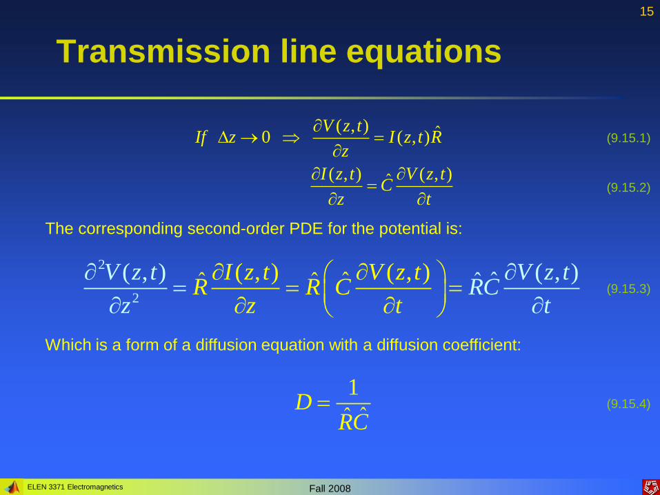
Transmission line equations
( , ) ˆ0 ( , )
( , ) ( , )ˆ
V z tIf z I z t R
z
I z t V z tC
z t
The corresponding second-order PDE for the potential is:
2
2
( , )( , ) ( , )ˆ( ,ˆ ˆ)ˆˆI z t V z tR R
V z t V z tRC
zC
z t t
(9.15.2)
(9.15.1)
(9.15.3)
Which is a form of a diffusion equation with a diffusion coefficient:
1
ˆˆD
RC (9.15.4)

ELEN 3371 Electromagnetics Fall 2008
16
Transmission line equations
Example 9.2: Show that a particular solution for the diffusion equation is given by 2
41
( , )2
z
DtV z t eD t
Differentiating the solution with respect to z: 2
43 2
( , ) 1
22
z
DtV z t z
ez DtD
2
2 2
42 3 2 2 5 2
( , ) 1
2 42
z
DtV z t z z
ez Dt D tD
Differentiating the solution with respect to t:
22
43 2 5 2
1 ( , ) 1 1
2 42
z
DtV z t t z
eD t D t DtD
(9.16.1)
(9.16.2)
(9.16.3)
(9.16.4)

ELEN 3371 Electromagnetics Fall 2008
17
Transmission line equations
Since the RHSs of (9.16.3) and (9.16.4) are equal, the diffusion equation is
satisfied.
The voltages at different times
are shown. The total area under
each curve equals 1.
This solution would be valid if a
certain amount of charge is
placed at z = 0 at some moment
in the past.
Note: the diffusion is significantly
different from the wave
propagation.

ELEN 3371 Electromagnetics Fall 2008
18
Sinusoidal waves
We are looking for the solutions of wave equations (9.13.1) and
(9.13.2) for the time-harmonic (AC) case. We must emphasize that –
unlike the solution for a static DC case or quasi-static low-frequency
case (ones considered in the circuit theory) – these solutions will be in
form of traveling waves of voltage and current, propagating in either
direction on the transmission line with the velocity specified by (9.13.3).
We assume here that the transmission line is connected to a distant generator
that produces a sinusoidal signal at fixed frequency = 2f. Moreover, the
generator has been turned on some time ago to ensure that transient response
decayed to zero; therefore, the line is in a steady-state mode.
The most important (and traditional) simplification for the time-harmonic case
is the use of phasors. We emphasize that while in the AC circuits analysis
phasors are just complex numbers, for the transmission lines, phasors are
complex functions of the position z on the line.

ELEN 3371 Electromagnetics Fall 2008
19
Sinusoidal waves
( , ) Re ( ) ; ( , ) Re ( )j t j tV z t V z e I z t I z e
22
2
22
2
( )( ) 0
( )( ) 0
d V zk V z
dz
d I zk I z
dz
Therefore, the wave equations will become:
Here, as previously, k is the wave number:
2k
v
Velocity of propagation
Wavelength of the voltage or current wave
(9.19.1)
(9.19.2)
(9.19.3)
(9.19.4)

ELEN 3371 Electromagnetics Fall 2008
20
Sinusoidal waves
A solution for the wave equation (9.13.3) can be found, for instance, in one of
these forms:
1 1
2 2
( ) cos sin
( ) jkz jkz
V z A kz B kz
V z A e B e
(9.20.1)
(9.20.2)
We select the exponential form (9.20.2) since it is easier to interpret in terms of
propagating waves of voltage on the transmission line.
Example 9.3: The voltage of a wave propagating through a transmission line was
continuously measured by a set of detectors placed at different locations along
the transmission line. The measured values are plotted. Write an expression for
the wave for the given data.

ELEN 3371 Electromagnetics Fall 2008
21
Sinusoidal waves
Slo
pe o
f th
e tra
jecto
ry…
The d
ata

ELEN 3371 Electromagnetics Fall 2008
22
Sinusoidal waves
We assume that the peak-to peak amplitude of the wave is 2V0. We also
conclude that the wave propagates in the +z direction.
The period of the wave is 2s, therefore, the frequency of oscillations is ½ Hz.
The velocity of propagation can be found from the slope as:
5 14
1 0v m s
The wave number is: 12 0.5
4 4k m
v
The wavelength is: 2 4 2
8 mk
Therefore, the wave is: 4
0( , )
zj t
V z t V e
(9.22.2)
(9.22.3)
(9.22.4)
(9.22.5)
Not in vacuum!
2 f (9.22.1)

ELEN 3371 Electromagnetics Fall 2008
23
Sinusoidal waves
Assuming next that the source is located far from the observation point (say, at z
= -) and that the transmission line is infinitely long, there would be only a
forward traveling wave of voltage on the transmission line. In this case, the
voltage on the transmission line is:
0( ) jkzV z V e
The phasor form of (9.12.3) in this case is
ˆ((
))
) (jkV z j LI zdV z
dz
0( ) ( )ˆ ˆ
jkzk kI z V z V e
L L
Which may be rearranged as:
(9.23.1)
(9.23.2)
(9.23.3)

ELEN 3371 Electromagnetics Fall 2008
24
Sinusoidal waves
The ratio of the voltage to the current is a very important transmission line
parameter called the characteristic impedance:
ˆ( )
( )c
V z LZ
I z k
1
ˆˆk and v
v LC
Since
Then: ˆ
ˆc
LZ
C
(9.24.1)
(9.24.2)
(9.24.3)
We emphasize that (9.24.3) is valid for the case when only one wave (traveling
either forwards or backwards) exists. In a general case, more complicated
expression must be used. If the transmission line was lossy, the characteristic
impedance would be complex.

ELEN 3371 Electromagnetics Fall 2008
25
Sinusoidal waves
If we know the characteristics of the transmission lane and the forward voltage
wave, we may find the forward current wave by dividing voltage by the
characteristic impedance.
Another important parameter of a transmission line is its length L, which is often
normalized by the wavelength of the propagation wave.
Assuming that the dielectric between conductors has and

ELEN 3371 Electromagnetics Fall 2008
26
Sinusoidal waves
The velocity of propagation does not depend on the dimensions of
the transmission line and is only a function of the parameters of the
material that separates two conductors. However, the characteristic
impedance DOES depend upon the geometry and physical
dimensions of the transmission line.

ELEN 3371 Electromagnetics Fall 2008
27
Sinusoidal waves
Example 9.4: Evaluate the velocity of propagation and the characteristic impedance
of an air-filled coaxial cable with radii of the conductors of 3 mm and 6 mm.
The inductance and capacitance per unit length are:
The velocity of propagation is:
The characteristic impedance of the cable is:
Both the v and the Zc may be decreased by insertion of a dielectric between leads.
7
0 4 10 6ˆ ln ln 0.142 2 3
H mb
La
12
02 2 8.854 10ˆ 80ln ln 6 3
pF mCb a
8
6 12
1 13 10
ˆˆ 0.14 10 80 10m sv
LC
6 12ˆˆ 0.14 10 80 10 42cZ L C
(9.27.1)
(9.27.2)
(9.27.3)
(9.27.4)

ELEN 3371 Electromagnetics Fall 2008
28
Terminators
So far, we assumed that the
transmission line was infinite. In
the reality, however,
transmission lines have both the
beginning and the end.
The line has a real characteristic
impedance Zc. We assume that the
source of the wave is at z = - and
the termination (the end of the line)
is at z = 0. The termination may be
either an impedance or another
transmission line with different
parameters. We also assume no
transients.

ELEN 3371 Electromagnetics Fall 2008
29
Terminators
The phasor voltage at any point on the line is:
2 2( ) jkz jkzV z A e B e
The phasor current is:
2 2( )jkz jkz
c
A e B eI z
Z
At the load location (z = 0), the ratio of voltage to current must be equal ZL:
2 2
2 2
( 0)
( 0)L c
A BV zZ Z
I z A B
Note: the ratio B2 to A2 represents the magnitude of the wave incident on the
load ZL.
(9.29.1)
(9.29.2)
(9.29.3)

ELEN 3371 Electromagnetics Fall 2008
30
Terminators
(9.30.1)
We introduce the reflection coefficient for the transmission line with a load as:
2
2
L c
L c
Z ZB
A Z Z
Often, the normalized impedance is used:
LL
c
Zz
Z
The reflection coefficient then becomes:
2
2
1
1
L
L
B z
A z
(9.30.2)
(9.30.3)

ELEN 3371 Electromagnetics Fall 2008
31
Terminators
Therefore, the phasor representations for the voltage and the current are:
0
0
( )
( )
jkz jkz
jkz jkz
c
V z V e e
VI z e e
Z
(9.31.1)
(9.31.2)
The total impedance is: ( )
( )( )
V zZ z
I z
generally a complicated function of the position and NOT equal to Zc. However,
a special case of matched load exists when:
L cZ Z
In this situation: ( ) cZ z Z
(9.31.3)
(9.31.4)
(9.31.5)

ELEN 3371 Electromagnetics Fall 2008
32
Terminators
Example 9.5: Evaluate the reflection coefficient for a wave that is incident from
z = - in an infinitely long coaxial cable that has r = 2 for z < 0 and r = 3 for z > 0.
The characteristic impedance is:
ˆ ln
ˆ 2c
b aLZ
C
The load impedance of a line is the characteristic impedance of the line for z > 0.

ELEN 3371 Electromagnetics Fall 2008
33
Terminators
The reflection coefficient can be expressed as:
0 0
2 0 1 02 1
2 1 0 0
2 0 1 0
2 1
2 1
ln ln
2 2
ln ln
2 2
1 1 1 1
3 20.1
1 1 1 1
3 2
r r
r r
r r
r r
b a b a
Z Z
Z Z b a b a

ELEN 3371 Electromagnetics Fall 2008
34
Terminators
The reflection coefficient is completely determined by the value of the
impedance of the load and the characteristic impedance of the transmission
line. The reflection coefficient for a lossless transmission line can have any
complex value with magnitude less or equal to one.
If the load is a short circuit (ZL = 0), the reflection coefficient = -1. The voltage
at the load is a sum of voltages of the incident and the reflected components
and must be equal to zero since the voltage across the short circuit is zero.
If the load is an open circuit (ZL = ), the reflection coefficient = +1. The
voltage at the load can be arbitrary but the total current must be zero.
If the load impedance is equal to the characteristic impedance (ZL = Zc), the
reflection coefficient = 0 – line is matched. In this case, all energy of
generator will be absorbed by the load.

ELEN 3371 Electromagnetics Fall 2008
35
Terminators
For the shorten transmission line:
0
0
1
( , ) Re
2 sin cos2
jkz jkz j tV z t V e e e
V kz t
(9.35.1)
(9.35.2)
For the open transmission line:
0
0
1
( , ) Re
2 cos cos
jkz jkz j tV z t V e e e
V kz t
(9.35.3)
(9.35.4)
In both cases, a standing wave is created.
The signal does not appear to propagate.

ELEN 3371 Electromagnetics Fall 2008
36
Terminators
Since the current can be found as 0 0 cI V Z
ZL =
ZL = 0
Note that the current wave differs from the voltage wave by 900

ELEN 3371 Electromagnetics Fall 2008
37
Terminators
Another important quantity is the ratio of the maximum voltage to the minimum
voltage called the voltage standing wave ratio:
max
min
1
1
VVSWR
V
Which leads to 1
1
VSWR
VSWR
VSWR, the reflection coefficient, the load impedance, and the characteristic
impedance are related.
Even when the amplitude of the incident wave V0 does not exceed the maximally
allowed value for the transmission line, reflection may lead to the voltage V0(1+||)
exceeding the maximally allowed.
Therefore, the load and the line must be matched.
(9.37.1)
(9.37.2)

ELEN 3371 Electromagnetics Fall 2008
38
Terminators
Example 9.6: Evaluate the VSWR for the coaxial cable described in the Example
9.5. The reflection coefficient was evaluated as = -0.1.
1 1 0.11.2
1 1 0.1VSWR
Note: if two cables were matched, the VSWR would be 1.

ELEN 3371 Electromagnetics Fall 2008
39
Terminators

ELEN 3371 Electromagnetics Fall 2008
40
Lossy transmission lines
Up to this point, our discussion was limited to lossless transmission lines
consisting of equivalent inductors and capacitors only. As a result, the
characteristic impedance for such lines is real. Let us incorporate ohmic
losses within the conductors and leakage currents between conductors.
In this case, the characteristic impedance becomes complex and the new
model will be:

ELEN 3371 Electromagnetics Fall 2008
41
Lossy transmission lines
The new first-order PDEs (telegrapher’s equations) are
( , ) ( , )ˆ ˆ ( , )
( , ) ( , )ˆ ˆ ( , )
I z t V z tC GV z t
z t
V z t I z tL RI z t
z t
(9.83.1)
(9.83.2)
Where the circuit elements are defines as
ˆ ˆˆ ˆ; ; ;L C R G
L C R Gz z z z
A time-harmonic excitation of the transmission line leads to a phasor notation:
( ) ˆ ˆ ( )
( ) ˆ ˆ ( )
I zG j C V z
z
V zR j L I z
z
(9.83.3)
(9.83.4)
(9.83.5)

ELEN 3371 Electromagnetics Fall 2008
42
Lossy transmission lines
The quantities in square brackets are denoted by distributed admittance and
distributed impedance leading to Y
Z
( ) ˆ ( )
( ) ˆ ( )
dI zYV z
dz
dV zZI z
dz
(9.84.1)
(9.84.2)
Second-order ODEs can be derived for current and voltage:
2
2
2
2
( ) ˆ ˆ ( )
( ) ˆ ˆ ( )
d I zZYI z
dz
d V zZYV z
dz
(9.84.3)
(9.84.4)
The phasor form solutions:
1 2
1 2
( )
( )
z z
z z
V z V e V e
I z I e I e
(9.84.5)
(9.84.6)

ELEN 3371 Electromagnetics Fall 2008
43
Lossy transmission lines
Here, is the complex propagation constant:
ˆ ˆˆ ˆ ˆ ˆj ZY R j L G j C (9.85.1)
As previously, we denote by V1 and I1 the amplitudes of the forward (in the +z
direction) propagating voltage and current waves; and V2 and I2 are the amplitudes
of the backward (in the -z direction) propagating voltage and current waves.
Therefore, the time varying waves will be in the form:
1 2
1 2
( , ) cos cos
( , ) cos cos
z z
z z
V z t V e t z V e t z
I z t I e t z I e t z
(9.85.2)
(9.85.3)
We recognize that (9.85.2) and (9.85.3) are exponentially decaying propagating
waves: the forward wave (V1, I1) propagates and decays in the +z direction, while
the backward wave (V2, I2) propagates and decays in the –z direction.

ELEN 3371 Electromagnetics Fall 2008
44
Lossy transmission lines
An example of a forward
propagating wave: it is
possible to determine the
values of and from the
graph as shown.

ELEN 3371 Electromagnetics Fall 2008
45
Lossy transmission lines
For small losses, employing a binomial approximation (1 – x)n 1 – nx for x << 1,
the complex propagating constant is approximately
ˆ ˆˆ ˆˆ ˆˆ ˆ1 1 1
ˆ ˆ ˆ ˆ2 2
R G R Gj j L j C j LC j
j L Lj C C
The attenuation constant can be approximated as
ˆ ˆˆ ˆ1ˆ ˆˆ ˆˆ ˆ ˆ ˆ22 2
R G R GLC LC
L LC C
The attenuation constant does not depend on frequency.
(9.87.1)
(9.87.2)

ELEN 3371 Electromagnetics Fall 2008
46
Lossy transmission lines (Ex)
Example 9.17: Find the complex propagation constant if the circuit elements satisfy
the ratio . Interpret this situation. ˆ ˆˆ ˆR L G C
The complex propagation constant is:
ˆ ˆˆ
ˆ ˆ ˆˆ ˆ ˆ ˆ ˆ ˆˆ ˆ
RC Cj R j L G j C R j L j C R j L
L L
The attenuation constant is independent on frequency, which implies no distortion
of a signal as it propagates on this transmission line and a constant attenuation.
The characteristic impedance of this transmission line
ˆ ˆ ˆ ˆ ˆ ˆ
ˆ ˆ ˆ ˆˆ ˆˆ ˆc
Z R j L R j L LZ
Y G j C CRC L j C
does not depend on frequency. Therefore, this transmission line is distortionless.

ELEN 3371 Electromagnetics Fall 2008
47
Lossy transmission lines
Example 9.18: The attenuation on a 50 distortionless transmission line is 0.01
dB/m. The line has a capacitance of 0.110-9 F/m. Find:
a) Transmission line parameters: distributed inductance, resistance, conductance;
b) The velocity of wave propagation.
Since the line is distortionless, the characteristic impedance is
2 2 9 7ˆ
ˆˆ50 50 0.1 10 2.5 10ˆc c
LZ L Z C H m
C
The attenuation constant is:
ˆ 0.01ˆ 0.01 1 20lg( ) 8.686 0.0012ˆ 8.686
CR dB m Np m e dB m Np m
L
Therefore: ˆ
ˆ 0.0012 50 0.0575ˆ c
LR Z m
C

ELEN 3371 Electromagnetics Fall 2008
48
Lossy transmission lines (Ex)
The distortionless line criterium is:
5
2 2
ˆ ˆˆ ˆ ˆ 0.0575ˆ 2.3 10ˆ ˆ ˆ 50c
R G RC RG S m
ZL LC
The phase velocity is:
8
7 9
1 12 10
ˆˆ 2.5 10 0.1 10v m s
LC

ELEN 3371 Electromagnetics Fall 2008
49
Dispersion and group velocity
The losses of types considered previously (finite conductivity of conductors and
nonzero conductivity of real dielectrics) lead to attenuation of wave amplitude as
it propagates through the line.
When the wavelength is comparable with the physical dimensions of the line or
when the permittivity of the dielectric depends on the frequency, another
phenomenon called dispersion occurs.
We will model dispersion by the
insertion of a distributed parasitic
capacitance in parallel to the distributed
inductance.
While developing the telegrapher’s
equation for this case, we note that the
current entering the node will split into
two portions:
( , ) ( , ) ( , )L cI z t I z t I z t (9.91.1)

ELEN 3371 Electromagnetics Fall 2008
50
Dispersion and group velocity
The voltage drop across the capacitor is:
( , )( , ) ˆ LI z tV z tL
z t
The voltage drop across the parasitic (shunt) capacitor is:
( , ) 1
ˆ c
s
V z tI dt
z C
Note: the units of this additional shunt capacitance are Fm rather than F/m.
The current passing through the shunt capacitor:
( , ) ( , )ˆI z t V z tC
z t
The wave equation will be:
2 2 4
2 2 2 2
( , ) ( , ) ( , )ˆ ˆˆ ˆ 0s
V z t V z t V z tLC LC
z t z t
(9.92.1)
(9.92.2)
(9.92.3)
(9.92.4)

ELEN 3371 Electromagnetics Fall 2008
51
Dispersion and group velocity
Assume that there is a time-harmonic signal generator connected to the
infinitely long transmission line. The complex time-varying wave propagating
through the line will be
( )
0( , ) j t zV z t V e
Combining (9.92.4) and (9.93.1) leads to the dispersion relation (the terms in the
square brackets) relating the propagation constant to the frequency of the wave:
2 2 2 2( )
0ˆ ˆˆ ˆ 0j t z
sV e j LC j LC j j
Therefore, the propagation constant is a nonlinear function of frequency:
2
ˆˆ
ˆˆ1 s
LC
LC
(9.93.1)
(9.93.2)
(9.93.3)

ELEN 3371 Electromagnetics Fall 2008
52
Dispersion and group velocity
dispersion
no dispersion
The propagation constant
depends on frequency – this
phenomenon is called
dispersion.
The phase velocity is a function
of frequency also.

ELEN 3371 Electromagnetics Fall 2008
53
Dispersion and group velocity
We can consider dispersion as a low pass filter acting on a signal. The
propagation constant will be a real number for frequencies less than the particular
cutoff frequency 0.
0
1
ˆˆsLC
This cutoff frequency is equal to the resonant frequency of the “tank” circuit. Above
this frequency, the propagation constant will be imaginary, and the wave will not
propagate.
In the non-dispersive frequency range (below the cutoff frequency), the velocity of
propagation is
0
1
ˆˆV
LC
The wave number below the cutoff frequency is:
00
0v
(9.95.1)
(9.95.2)
(9.95.3)

ELEN 3371 Electromagnetics Fall 2008
54
Dispersion and group velocity
Dispersion implies that
the propagation
constant depends on
the frequency.
There are positive and
negative dispersions.
Note that in the case of
negative dispersion,
waves of frequencies
less than a certain cutoff
frequency will propagate.
While for the positive dispersion, only the waves whose frequency exceeds the
cutoff frequency will propagate.
ELEN 3371 Electromagnetics Fall 2008
55
Dispersion and group velocity
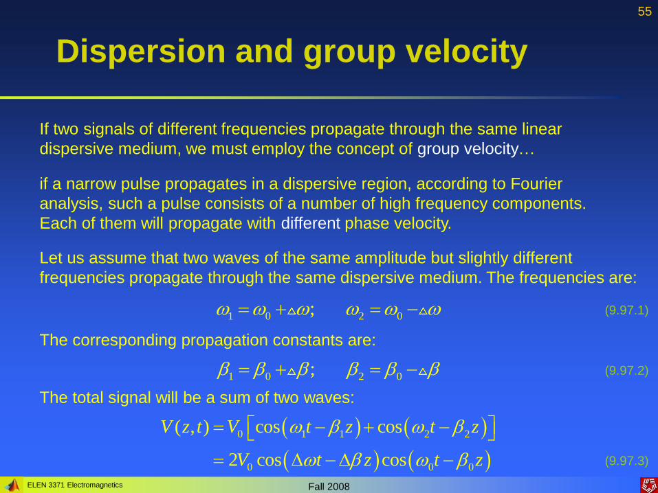
If two signals of different frequencies propagate through the same linear
dispersive medium, we must employ the concept of group velocity…
if a narrow pulse propagates in a dispersive region, according to Fourier
analysis, such a pulse consists of a number of high frequency components.
Each of them will propagate with different phase velocity.
Let us assume that two waves of the same amplitude but slightly different
frequencies propagate through the same dispersive medium. The frequencies are:
1 0 2 0;
The corresponding propagation constants are:
1 0 2 0;
The total signal will be a sum of two waves:
0 1 1 2 2
0 0 0
( , ) cos cos
2 cos cos
V z t V t z t z
V t z t z
(9.97.1)
(9.97.2)
(9.97.3)

ELEN 3371 Electromagnetics Fall 2008
56
Dispersion and group velocity
Summation of two time-harmonic
waves of slightly different
frequencies leads to constructive
and destructive interference.
voltage
By detecting signals at two locations, we
can track a point of constant phase
propagating with the phase velocity:
0 0pv
and the peak of the envelope propagating with the group velocity: gv
(9.98.1)
(9.98.2)
In dispersive media, phase and group velocities can be considerably different!

ELEN 3371 Electromagnetics Fall 2008
57
Dispersion and group velocity (Ex)
Example 9.19: Find the phase and group velocities for:
a) Normal transmission line;
b) A line in which the elements are interchanged.
a) The propagation
constant computed
according to (9.87.1)
will be:
ˆ ˆˆ ˆ ˆ ˆj YZ j L j C j LC
The phase velocity is 1
ˆˆpv
LC
The group velocity is 11
ˆˆgv
LC

ELEN 3371 Electromagnetics Fall 2008
58
Dispersion and group velocity (Ex)
The two velocities are equal in this case and both are independent on frequency.
b) The propagation constant computed according to (9.87.1) will be:
1 1 1ˆ ˆˆ ˆ ˆˆ
j YZj Lj C j LC
The phase velocity is 2 ˆˆ
pv LC
The group velocity is 2 ˆˆ1gv LC
The phase and group velocities both depend on frequency and are in the
opposite directions.
?? QUESTIONS ??