Lecture 8Lecture 8 Today Continue with Dimensionality Reduction Last lecture: PCA This lecture:...

CS434a/541a: Pattern RecognitionProf. Olga Veksler

Lecture 8

Today

� Continue with Dimensionality Reduction� Last lecture: PCA� This lecture: Fisher Linear Discriminant

� PCA finds the most accurate data representationin a lower dimensional space� Project data in the directions of maximum variance

� Fisher Linear Discriminant project to a line which preserves direction useful for data classification

Data Representation vs. Data Classification

� However the directions of maximum variance may be useless for classification

apply PCA

to each class

separable

not separable

Fisher Linear Discriminant

� Main idea: find projection to a line s.t. samples from different classes are well separated

bad line to project to,classes are mixed up

Example in 2D

good line to project to,classes are well separated

Fisher Linear Discriminant� Suppose we have 2 classes and d-dimensional

samples x1,…,xn where � n1 samples come from the first class� n2 samples come from the second class

� consider projection on a line� Let the line direction be given by unit vector v

vixvt x

i

� Scalar vtxi is the distance of projection of xi from the origin

� Thus it vtxi is the projection of xi into a one dimensional subspace


� How to measure separation between projections of different classes?

� Thus the projection of sample xi onto a line in direction v is given by vtxi

�� ∈∈∈∈ ∈∈∈∈

====��

��

��========

1 1

11

1111

11~n

Cx

tn

Cxi

ti

t

i i

vxn

vxvn

µµµµµµµµ

� Let µµµµ1 and µµµµ2 be the means of classes 1 and 2

� Let and be the means of projections of classes 1 and 2

1~µµµµ 2

~µµµµ

22~, µµµµµµµµ tvsimilarly ====

� seems like a good measure21~~ µµµµµµµµ −−−−


� How good is as a measure of separation?� The larger , the better is the expected separation

21~~ µµµµµµµµ −−−−

� the vertical axes is a better line than the horizontal axes to project to for class separability

� however 2121~~ µµµµµµµµµµµµµµµµ −−−−>>>>−−−− ��


1µµµµ

2µµµµ

1µµµµ�2µµµµ�

1~µµµµ

2~µµµµ


� The problem with is that it does not consider the variance of the classes


1µµµµ�2µµµµ�

1~µµµµ

2~µµµµ

large variance

smal

l var

ianc

e

1µµµµ

2µµµµ


� We need to normalize by a factor which is proportional to variance


(((( ))))��====

−−−−====n

izizs

1

2µµµµ

� Define their scatter as

� Have samples z1,…,zn . Sample mean is ��====

====n

iiz z

n 1

1µµµµ

� Thus scatter is just sample variance multiplied by n� scatter measures the same thing as variance, the spread

of data around the mean� scatter is just on different scale than variance

larger scatter: smaller scatter:


� Fisher Solution: normalize by scatter21~~ µµµµµµµµ −−−−

(((( ))))��∈∈∈∈

−−−−====2Classy

22i

22

i

~ys~ µµµµ� Scatter for projected samples of class 2 is

� Scatter for projected samples of class 1 is (((( ))))��

∈∈∈∈

−−−−====1

21

21

~~Classy

ii

ys µµµµ

� Let yi = vtxi , i.e. yi ‘s are the projected samples


� We need to normalize by both scatter of class 1 and scatter of class 2

(((( )))) (((( ))))22

21

221

~~~~

ssvJ

++++−−−−====

µµµµµµµµ

� Thus Fisher linear discriminant is to project on line in the direction v which maximizes

want projected means are far from each other

want scatter in class 2 is as small as possible, i.e. samples of class 2 cluster around the projected mean 2

~µµµµ

want scatter in class 1 is as small as possible, i.e. samples of class 1 cluster around the projected mean 1

~µµµµ


(((( )))) (((( ))))22

21

221

~~~~

ssvJ

++++−−−−====

µµµµµµµµ

� If we find v which makes J(v) large, we are guaranteed that the classes are well separated

1~µµµµ

2~µµµµ

small implies that projected samples of class 1 are clustered around projected mean

1~s small implies that

projected samples of class 2 are clustered around projected mean

2~s

projected means are far from each other

Fisher Linear Discriminant Derivation

� All we need to do now is to express J explicitly as a function of v and maximize it� straightforward but need linear algebra and Calculus

(((( )))) (((( ))))22

21

221

~~~~

ssvJ

++++−−−−====

µµµµµµµµ

� Define the separate class scatter matrices S1 and S2 for classes 1 and 2. These measure the scatter of original samples xi (before projection)

(((( ))))(((( ))))��∈∈∈∈

−−−−−−−−====1

111Classx

tii

i

xxS µµµµµµµµ

(((( ))))(((( ))))��∈∈∈∈

−−−−−−−−====2

222Classx

tii

i

xxS µµµµµµµµ


� Now define the within the class scatter matrix21 SSSW ++++====

� Recall that (((( ))))��∈∈∈∈

−−−−====1

21

21

~~Classy

ii

ys µµµµ

(((( ))))��∈∈∈∈

−−−−====1Classy

21

ti

t21

i

vxvs~ µµµµ

� Using yi = vtxi and 11~ µµµµµµµµ tv====

(((( ))))(((( )))) (((( ))))(((( ))))��∈∈∈∈

−−−−−−−−====1Classy

t1i

tt1i

i

vxvx µµµµµµµµ

(((( ))))(((( ))))��∈∈∈∈

−−−−−−−−====1Classy

t1i1i

t

i

vxxv µµµµµµµµ vSv t1====

(((( ))))(((( )))) (((( ))))(((( ))))��∈∈∈∈

−−−−−−−−====1Classy

1itt

1it

i

xvxv µµµµµµµµ


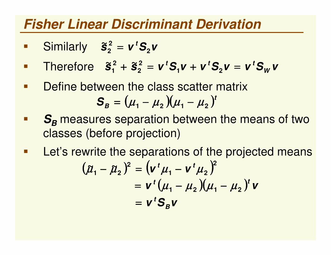
� Similarly vSvs t2

22

~ ====

� Let’s rewrite the separations of the projected means

� Therefore vSvvSvvSvss Wttt ====++++====++++ 21

22

21

~~

(((( )))) (((( ))))221

221

~~ µµµµµµµµµµµµµµµµ tt vv −−−−====−−−−(((( ))))(((( )))) vv tt

2121 µµµµµµµµµµµµµµµµ −−−−−−−−====vSv B

t====

� Define between the class scatter matrix(((( ))))(((( ))))t

BS 2121 µµµµµµµµµµµµµµµµ −−−−−−−−====� SB measures separation between the means of two

classes (before projection)


� Thus our objective function can be written:

� Minimize J(v) by taking the derivative w.r.t. v and setting it to 0

(((( )))) (((( ))))2vSv

vSvvSvdvdvSvvSv

dvd

vJdvd

Wt

Bt

Wt

Wt

Bt

��

��

��−−−−��

��

��

====

(((( )))) (((( ))))(((( ))))2

22

vSv

vSvvSvSvvS

Wt

Bt

WWt

B −−−−==== 0====

(((( )))) (((( ))))vSvvSv

s~s~~~

vJW

tB

t

22

21

221 ====

++++−−−−====

µµµµµµµµ


� Need to solve (((( )))) (((( )))) 0====−−−− vSvSvvSvSv WBt

BWt

(((( )))) (((( ))))0====−−−−��

vSvvSvSv

vSvvSvSv

Wt

WBt

Wt

BWt

(((( ))))0====−−−−��

vSvvSvSv

vSW

tWB

t

B

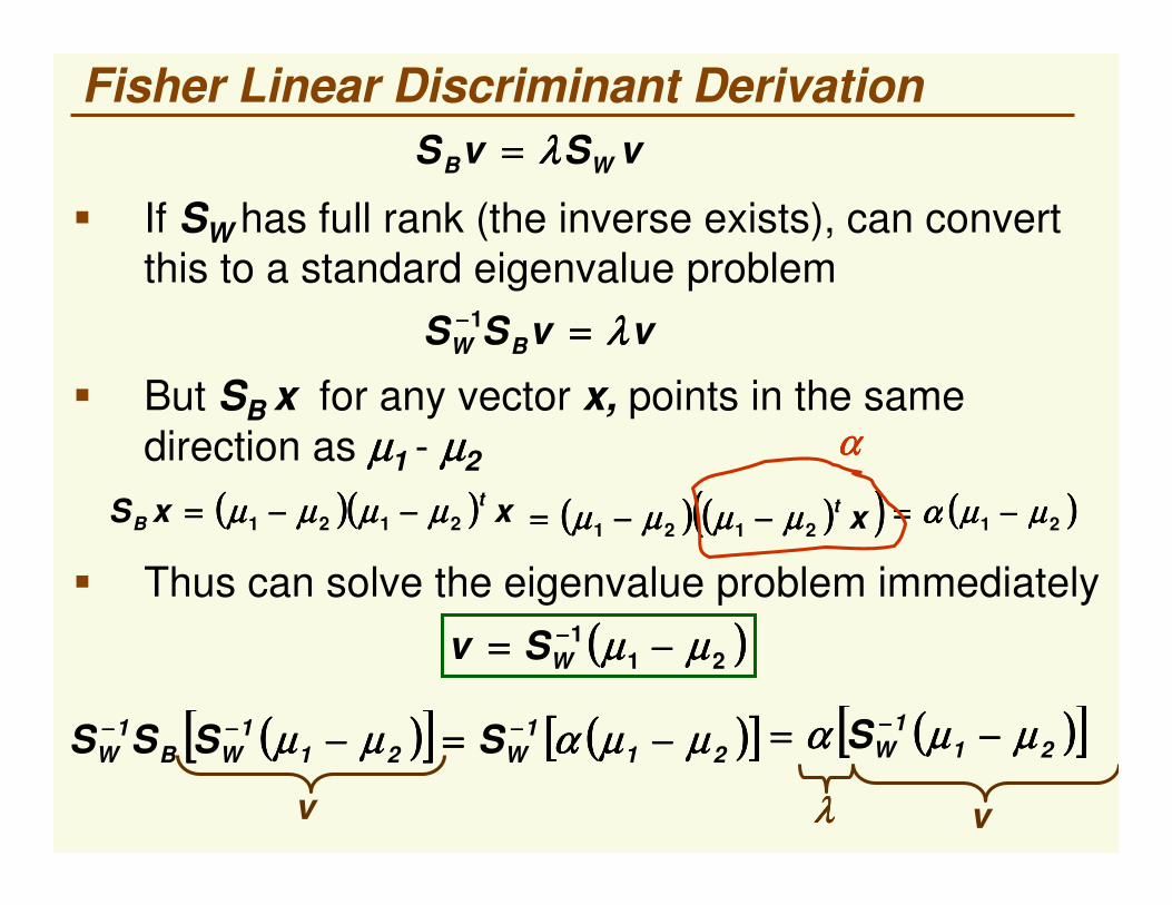
vSvS WB λλλλ====��

λλλλ====

generalized eigenvalue problem


� If SW has full rank (the inverse exists), can convert this to a standard eigenvalue problem

vSvS WB λλλλ====

vvSS BW λλλλ====−−−−1

� But SB x for any vector x, points in the same direction as µµµµ1 - µµµµ2

(((( ))))(((( )))) xxS tB 2121 µµµµµµµµµµµµµµµµ −−−−−−−−==== (((( )))) (((( ))))(((( ))))xt

2121 µµµµµµµµµµµµµµµµ −−−−−−−−==== (((( ))))21 µµµµµµµµαααα −−−−====

� Thus can solve the eigenvalue problem immediately (((( ))))21

1 µµµµµµµµ −−−−==== −−−−WSv

αααα

(((( ))))[[[[ ]]]] (((( ))))[[[[ ]]]]211

W211

WB1

W SSSS µµµµµµµµααααµµµµµµµµ −−−−====−−−− −−−−−−−−−−−−

v v

(((( ))))[[[[ ]]]]211

WS µµµµµµµµαααα −−−−==== −−−−

λλλλ

Fisher Linear Discriminant Example� Data

� Class 1 has 5 samples c1=[(1,2),(2,3),(3,3),(4,5),(5,5)]� Class 2 has 6 samples c2=[(1,0),(2,1),(3,1),(3,2),(5,3),(6,5)]

� Arrange data in 2 separate matrices

��

��

��====

55

21c1 ��

��

��

��====

56

01c2 ��

� Notice that PCA performs very poorly on this data because the direction of largest variance is not helpful for classification

Fisher Linear Discriminant Example

� First compute the mean for each class(((( )))) [[[[ ]]]]6.33cmean 11 ========µµµµ (((( )))) [[[[ ]]]]23.3cmean 22 ========µµµµ

(((( ))))��

�� ====∗∗∗∗==== 2.70.8

0.810ccov4S 11 (((( ))))��

�� ====∗∗∗∗==== 1616

163.17ccov5S 22

� Compute scatter matrices S1 and S2 for each class

��

�� ====++++==== 2.2324

243.27SSS 21W

� Within the class scatter:

� it has full rank, don’t have to solve for eigenvalues

(((( ))))��

�� −−−−

−−−−========−−−−47.041.041.039.0SinvS W

1W� The inverse of SW is

� Finally, the optimal line direction v(((( ))))

��

�� −−−−====−−−−==== −−−−

89.079.0Sv 21

1W µµµµµµµµ

Fisher Linear Discriminant Example

� Notice, as long as the line has the right direction, its exact position does not matter

� Last step is to compute the actual 1D vector y. Let’s do it separately for each class

[[[[ ]]]] [[[[ ]]]]4.081.0525173.065.011 �

�� ====

��

�� −−−−======== ttcvY

[[[[ ]]]] [[[[ ]]]]25.065.0506173.065.022 −−−−−−−−====��

�� −−−−======== �

��ttcvY

Multiple Discriminant Analysis (MDA)� Can generalize FLD to multiple classes� In case of c classes, can reduce dimensionality to

1, 2, 3,…, c-1 dimensions� Project sample xi to a linear subspace yi = V txi

� V is called projection matrix

Multiple Discriminant Analysis (MDA)

� Objective function: (((( )))) (((( ))))(((( ))))VSVdet

VSVdetVJ

Wt

Bt

====

� within the class scatter matrix SW is

(((( ))))(((( ))))�� ==== ∈∈∈∈====

−−−−−−−−========c

1i

tik

iclassxik

c

1iiW xxSS

k

µµµµµµµµ

� between the class scatter matrix SB is

(((( ))))(((( ))))ti

c

1iiiB nS µµµµµµµµµµµµµµµµ −−−−−−−−==== ��

====

� Let

��∈∈∈∈

====iclassxi

i xn1µµµµ ��====

ixix

n1µµµµ

maximum rank is c -1

� ni by the number of samples of class i� and µµµµi be the sample mean of class i� µ µ µ µ be the total mean of all samples

Multiple Discriminant Analysis (MDA)

(((( )))) (((( ))))(((( ))))VSVdet

VSVdetVJ

Wt

Bt

====

� The optimal projection matrix V to a subspace of dimension k is given by the eigenvectors corresponding to the largest k eigenvalues

� First solve the generalized eigenvalue problem:vSvS WB λλλλ====

� At most c-1 distinct solution eigenvalues

� Let v1, v2 ,…, vc-1 be the corresponding eigenvectors

� Thus can project to a subspace of dimension at most c-1

FDA and MDA Drawbacks� Reduces dimension only to k = c-1 (unlike PCA)

� For complex data, projection to even the best line may result in unseparable projected samples

� Will fail:1. J(v) is always 0: happens if µµµµ1 = µµµµ2

PCA performs reasonably well here:

PCA also fails:

2. If J(v) is always large: classes have large overlap when projected to any line (PCA will also fail)

Lecture 8Lecture 8 Today Continue with Dimensionality Reduction Last lecture: PCA This lecture:...

Documents

Transcript of Lecture 8Lecture 8 Today Continue with Dimensionality Reduction Last lecture: PCA This lecture:...